1

Improved Graph ClusteringYudong Chen, Sujay Sanghavi, and Huan Xu

Abstract—Graph clustering involves the task of dividing nodesinto clusters, so that the edge density is higher within clustersas opposed to across clusters. A natural, classic and popularstatistical setting for evaluating solutions to this problem is thestochastic block model, also referred to as the planted partitionmodel.

In this paper we present a new algorithm—a convexifiedversion of Maximum Likelihood—for graph clustering. We showthat, in the classic stochastic block model setting, it outperformsexisting methods by polynomial factors when the cluster size isallowed to have general scalings. In fact, it is within logarithmicfactors of known lower bounds for spectral methods, and thereis evidence suggesting that no polynomial time algorithm woulddo significantly better.

We then show that this guarantee carries over to a moregeneral extension of the stochastic block model. Our method canhandle the settings of semi-random graphs, heterogeneous degreedistributions, unequal cluster sizes, unaffiliated nodes, partiallyobserved graphs and planted clique/coloring etc. In particular,our results provide the best exact recovery guarantees to datefor the planted partition, planted k-disjoint-cliques and plantednoisy coloring models with general cluster sizes; in other settings,we match the best existing results up to logarithmic factors.

I. INTRODUCTION

This paper proposes a new algorithm for the following task:given an undirected unweighted graph, assign the nodes intodisjoint clusters so that the density of edges within clustersis higher than the edge density across clusters. Clusteringarises in applications such as a community detection, userprofiling, link prediction, collaborative filtering etc. In theseapplications, one is often given as input a set of similarityrelationships (either “1” or “0”) and the goal is to identifygroups of similar objects. For example, given the friendshiprelations on Facebook, one would like to detect tightly con-nected communities, which is useful for subsequent tasks likecustomized recommendation and advertisement.

Graphs in modern applications have several characteristicsthat complicate graph clustering:

The work of Y. Chen was supported by NSF grant EECS-1056028 andDTRA grant HDTRA 1-08-0029. The work of S. Sanghavi was supportedby the DTRA Young investigator award and NSF grants 1302435, 1017525and 0954059. The work of H. Xu was partially supported by the Ministry ofEducation of Singapore through AcRF Tier Two grant R-265-000-443-112.The material in this paper was presented in part under the title “ClusteringSparse Graphs” at the Neural Information Processing Systems Conference,Lake Tahoe, Nevada, United States, 2012.

Y. Chen is with the Department of Electrical Engineering and Com-puter Sciences at the University of California at Berkeley, Berkeley, CA94720, USA. S. Sanghavi is with the Department of Electrical and Com-puter Engineering, The University of Texas at Austin, Austin, TX 78712,USA. H. Xu is with the Department of Mechanical Engineering, NationalUniversity of Singapore, 9 Engineering Drive 1, Singapore 117575, Sin-gapore. (e-mail: yudong.chen@eecs.berkeley.edu, sanghavi@mail.utexas.edu,mpexuh@nus.edu.sg)

• Small density gap: the edge density across clusters isonly a small additive or multiplicative factor differentfrom within clusters;

• Sparsity: the graph is overall very sparse even withinclusters;

• High dimensionality: the number of clusters may growunbounded as a function of the number of nodes n, whichmeans the sizes of the clusters can be vanishingly smallcompared to n;

• Unaffiliated nodes: there may exist a large number ofnodes that do not belong to any clusters and are looselyconnected to the rest of the graph;

• Heterogeneity: the cluster sizes, node degrees and edgedensities may be non-uniform across the graph; edgeconnections may not be well-modeled by a probabilis-tic distribution, and there may exist hierarchical clusterstructures.

Various large modern datasets and graphs have such char-acteristics [1, 2]; examples include the web graph and socialgraphs of various social networks etc. As has been well-recognized, these characteristics make clustering more dif-ficult. When the in-cluster and across-cluster edge densitiesare close or there are many unstructured unaffiliated nodes,the clustering structure is less significant and thus harder todetect. Sparsity further reduces the amount of information andmakes the problem noisier. In the high dimensional regime,there are many small clusters, which are easy to lose inthe noise. Heterogeneous and non-random structures in thegraphs foil many algorithms that otherwise perform well; forexample, conventional spectral clustering methods are oftenknown to be not robust to heterogeneity in the graphs [3, 4].Finally, the existence of hierarchical structures and unaffiliatednodes renders many existing algorithms and theoretical resultsinapplicable, as they fix the number of clusters a priori andforce each node to be assigned to a cluster. It is desirableto design an algorithm that can handle all these issues in aprincipled manner.

A. Our Contributions

Our algorithmic contribution is a new method for un-weighted graph clustering. It is motivated by the maximum-likelihood estimator for the classical Stochastic Block-model [5] (also known as the Planted Partition Model [6])for random clustered graphs. In particular, we show thatthis maximum-likelihood estimator can be written as a linearobjective over combinatorial constraints; our algorithm is aconvex relaxation of these constraints, yielding a convexprogram overall. While this is the motivation, it performswell—both in theory and empirically—in settings that are notjust the standard stochastic blockmodel.

arX

iv:1

210.

3335

v3 [

stat

.ML

] 6

Jan

201

5

2

Our main analytical result in this paper is theoreticalguarantees on our algorithm’s performance; we study it in asemi-random generalized stochastic blockmodel. This modelgeneralizes not only the standard stochastic blockmodel andplanted partition model, but many other classical planted mod-els including planted k-disjoint-cliques [7, 8], planted densesubgraph [9], planted coloring [10, 4] and their semi-randomvariants [11, 12, 13]. Our main result gives the conditions (asa function of the in/cross-cluster edge densities p and q, thedensity gap |p− q|, the minimum cluster size K and the totalnumber of nodes n) under which our algorithm is guaranteedto recover the ground-truth clustering. When p > q, the keycondition reads

p− q = Ω

(√p(1− q)nK

); (1)

here all the parameters are allowed to scale with n. Note thatthe condition does not depend explicitly on the number ofunaffiliated nodes or the number of clusters. An analogousresult holds for p < q.

While the planted and stochastic block models have arich literature, this single result shows that the performanceof our algorithm matches all existing methods (up to atmost logarithmic factors) in exact recovery; moreover, in thecases of the standard planted partition/k-disjoint-cliques/noisy-coloring models with general scaling of p, q and K, we achieveorder-wise improvement over existing methods, in the sensethat our algorithm succeeds for a much larger range of theparameters. In fact, there is evidence indicating that we areclose to the boundary at which any polynomial-time algorithmcan be expected to work. The proof for our main theoremis relatively simple, relying only on standard concentrationresults. Our simulation study supports our theoretic finding,that the proposed method is effective in clustering noisy graphsand outperforms existing methods.

The rest of the paper is organized as follows: Section I-Bprovides an overview of related work; Section II presents ouralgorithm; Section III describes the Semi-Random General-ized Stochastic Blockmodel, which is a generalization of thestandard stochastic blockmodel, one that allows the modelingof the issues mentioned above; Section IV presents the mainresults—a performance analysis of our algorithm for the semi-random generalized stochastic blockmodel, and provides adetailed comparison to the existing literature and a discussionof the implications for different special cases; Section Vprovides simulation results; the proofs of our theoretic resultsare given in Sections VI to IX; the paper concludes with adiscussion in Section X

B. Related Work

The general field of clustering, or even graph clustering, istoo vast for a detailed survey here; we focus on the mostrelated threads, and therein too primarily on work whichprovides analytical guarantees on the resulting algorithms.

1) Stochastic block models: Also called “planted mod-els” [5, 6], these are arguably the most natural randomclustered graph models. In the simplest or standard setting,

n nodes are partitioned into disjoint subsets of equal sizeK (called the true clusters), and then edges are generatedindependently and at random, with the probability p of anedge between two nodes in the same cluster higher than theprobability q for two nodes in different clusters. The task isto recover the true clusters given the graph. The parametersp, q,K and n typically govern whether an algorithm succeedsin recovery or not.

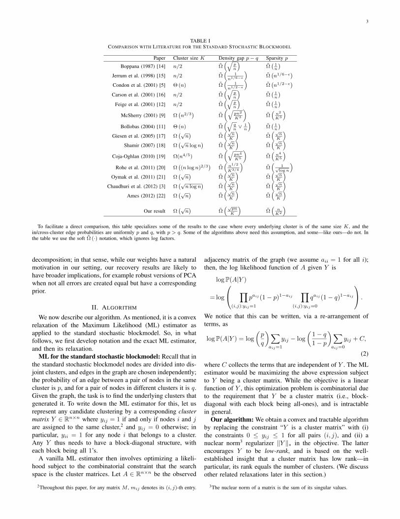
There is now a long line of analytical work on stochasticblock models; we focus on methods that allow for exact recov-ery (i.e., every node is correctly classified), and summarize theconditions required by known methods in Table I. As can beseen, we improve over existing methods by polynomial factorsfor general values of K—in particular, when the cluster sizesatisfies K = n1−α for any constant α > 0 (which meansthe number of clusters is growing at the rate n/K = nα.)1

In addition, as opposed to several of these methods, ourmethod can handle unaffiliated nodes, heterogeneity, hierarchyin clustering etc, and apply to other models including plantedclique and planted noisy coloring.

We would like to mention two recent results that appearedafter the conference version [23] of this paper. The workin [24] shows that a computationally efficient tensor decom-position approach succeeds for the standard stochastic block-model when p−q = Ω

(√pn polylog n/K

); our guarantee (1)

is better by a factor of Θ(polylog n/√

1− q). Moreover, forthe standard planted clique model (p = 1, q = 1/2), we onlyrequire the clique size to be K = Ω(

√n), better than their

requirement K = Ω(n2/3). Another subsequent work [25]considers the setting with heterogeneous cluster sizes andno unaffiliated nodes, and shows that our algorithm can becombined with an iterative reduction procedure to sequentiallyrecover clusters smaller than is allowed in this paper.

A complimentary line of work has investigated lowerbounds for the stochastic blockmodel; i.e., for what val-ues/scalings of p, q and K it is not possible (either for anyalgorithm, or for any polynomial-time algorithm) to recoverthe underlying true clusters [3, 26, 27]. We discuss andcompare with these two lines of work in more details in themain results section.

2) Convex methods for matrix decomposition: Our methodis related to recent literature on the recovery of low-rank matri-ces using convex optimization, and in particular the recoveryof such matrices from “sparse” perturbations (i.e., where afraction of the elements of the low-rank matrix are possiblyarbitrarily modified, while others are untouched). Sparse andlow-rank matrix decomposition using convex optimization wasinitiated by [28, 29]; follow-up works [30, 31] have the currentstate-of-the-art guarantees on this problem, and [32] applies itdirectly to graph clustering.

The method in this paper is Maximum Likelihood, but it canalso be viewed as a weighted version of sparse and low-rankmatrix decomposition, with different elements of the sparsepart penalized differently, based on the given input graph.There is currently little work or analysis on weighted matrix

1Our comparison focuses on polynomial factors and the setting with generalvalues of K. We note that in the special case of K = Θ(n), some existingresults (e.g.,[19]) are better then ours by logarithmic factors.

3

TABLE ICOMPARISON WITH LITERATURE FOR THE STANDARD STOCHASTIC BLOCKMODEL

Paper Cluster size K Density gap p− q Sparsity p

Boppana (1987) [14] n/2 Ω(√

pn

)Ω(1n

)Jerrum et al. (1998) [15] n/2 Ω

(1

n1/6−ε

)Ω(n1/6−ε)

Condon et al. (2001) [5] Θ (n) Ω(

1n1/2−ε

)Ω(n1/2−ε)

Carson et al. (2001) [16] n/2 Ω(√

pn

)Ω(1n

)Feige et al. (2001) [12] n/2 Ω

(√pn

)Ω(1n

)McSherry (2001) [9] Ω

(n2/3

)Ω

(√pn2

K3

)Ω(n2

K3

)Bollobas (2004) [11] Θ (n) Ω

(√qn∨ 1n

)Ω(1n

)Giesen et al. (2005) [17] Ω

(√n)

Ω(√

nK

)Ω(√

nK

)Shamir (2007) [18] Ω

(√n logn

)Ω(√

nK

)Ω(√

nK

)Coja-Oghlan (2010) [19] Ω(n4/5) Ω

(√pn4

K5

)Ω(n4

K5

)Rohe et al. (2011) [20] Ω

((n logn)2/3

)Ω(n1/2

K3/4

)Ω(

1√logn

)Oymak et al. (2011) [21] Ω

(√n)

Ω(√

nK

)Ω(√

nK

)Chaudhuri et al. (2012) [3] Ω

(√n logn

)Ω(√

nK

)Ω(√

nK

)Ames (2012) [22] Ω

(√n)

Ω(√

nK

)Ω(√

nK

)Our result Ω

(√n)

Ω(√

pn

K

)Ω(nK2

)To facilitate a direct comparison, this table specializes some of the results to the case where every underlying cluster is of the same size K, and the

in/cross-cluster edge probabilities are uniformly p and q, with p > q. Some of the algorithms above need this assumption, and some—like ours—do not. Inthe table we use the soft Ω (·) notation, which ignores log factors.

decomposition; in that sense, while our weights have a naturalmotivation in our setting, our recovery results are likely tohave broader implications, for example robust versions of PCAwhen not all errors are created equal but have a correspondingprior.

II. ALGORITHM

We now describe our algorithm. As mentioned, it is a convexrelaxation of the Maximum Likelihood (ML) estimator asapplied to the standard stochastic blockmodel. So, in whatfollows, we first develop notation and the exact ML estimator,and then its relaxation.

ML for the standard stochastic blockmodel: Recall that inthe standard stochastic blockmodel nodes are divided into dis-joint clusters, and edges in the graph are chosen independently;the probability of an edge between a pair of nodes in the samecluster is p, and for a pair of nodes in different clusters it is q.Given the graph, the task is to find the underlying clusters thatgenerated it. To write down the ML estimator for this, let usrepresent any candidate clustering by a corresponding clustermatrix Y ∈ Rn×n where yij = 1 if and only if nodes i and jare assigned to the same cluster,2 and yij = 0 otherwise; inparticular, yii = 1 for any node i that belongs to a cluster.Any Y thus needs to have a block-diagonal structure, witheach block being all 1’s.

A vanilla ML estimator then involves optimizing a likeli-hood subject to the combinatorial constraint that the searchspace is the cluster matrices. Let A ∈ Rn×n be the observed

2Throughout this paper, for any matrix M , mij denotes its (i, j)-th entry.

adjacency matrix of the graph (we assume aii = 1 for all i);then, the log likelihood function of A given Y is

logP(A|Y )

= log

∏(i,j):yij=1

paij (1− p)1−aij∏

(i,j):yij=0

qaij (1− q)1−aij

.

We notice that this can be written, via a re-arrangement ofterms, as

logP(A|Y ) = log

(p

q

)∑aij=1

yij − log

(1− q1− p

)∑aij=0

yij + C,

(2)

where C collects the terms that are independent of Y . The MLestimator would be maximizing the above expression subjectto Y being a cluster matrix. While the objective is a linearfunction of Y , this optimization problem is combinatorial dueto the requirement that Y be a cluster matrix (i.e., block-diagonal with each block being all-ones), and is intractablein general.

Our algorithm: We obtain a convex and tractable algorithmby replacing the constraint “Y is a cluster matrix” with (i)the constraints 0 ≤ yij ≤ 1 for all pairs (i, j), and (ii) anuclear norm3 regularizer ‖Y ‖∗ in the objective. The latterencourages Y to be low-rank, and is based on the well-established insight that a cluster matrix has low rank—inparticular, its rank equals the number of clusters. (We discussother related relaxations later in this section.)

3The nuclear norm of a matrix is the sum of its singular values.

4

Also notice that the likelihood expression (2) is linear inY and only the ratio of the two coefficients log(p/q) andlog((1 − q)/(1 − p)) is important. We therefore introduce aparameter t which allows us to choose any ratio. This has theadvantage that instead of knowing both p and q, we only needto choose one number t (which should be between p and q; weremark on how to choose t later). This leads to the followingconvex formulation:

maxY ∈Rn×n

cA∑aij=1

yij − cAc∑aij=0

yij − 48√n ‖Y ‖∗ (3)

s.t. 0 ≤ yij ≤ 1,∀i, j. (4)

where the weights cA and cAc are given by

cA =

√1− tt

and cAc =

√t

1− t. (5)

Here the factor 48√n balances the contributions of the nuclear

norm and the likelihood; the specific values of this factor aswell as of cA and cAc are derived from our analysis (cf.Section VII-E). The optimization problem (3)–(4) is convexand can be cast as a Semidefinite Program (SDP) [28, 33].More importantly, it can be solved using efficient first-ordermethods for large graphs (see Section V-A).

Our algorithm is given as Algorithm 1. Depending on thegiven A and the choice of t, the optimal solution Y may ormay not be a cluster matrix. Checking if a given Y is a clustermatrix can be done easily, e.g., via an SVD, which will alsoreveal the cluster memberships if it is a cluster matrix. If it isnot, any one of several rounding/aggregation ideas (e.g., theone in [34]) can be used empirically; we do not delve into thisapproach in this paper, and simply output failure. In Section IVwe provide sufficient conditions under which Y is guaranteedto be a cluster matrix, with no rounding required.

Algorithm 1 Convex ClusteringInput: A ∈ Rn×n, t ∈ (0, 1)Solve program (3)–(4) with weights (5). Let Y be an optimalsolution.if Y is a cluster matrix then

Output cluster memberships obtained from Y .else

Output “Failure”.end if

A. Remarks about the Algorithm

Note that while we derive our algorithm from the standardstochastic blockmodel, our analytical results hold in a muchmore general setting. In practice, one could execute thealgorithm (with appropriate choice of t, and hence cA andcAc ) on any given graph.

Tighter relaxations: The formulation (3)–(4) is not the onlyway to relax the non-convex ML estimator. Instead of thenuclear norm regularizer, a hard constraint ‖Y ‖∗ ≤ n may beused. One may further replace this constraint with the positivesemidefinite constraint Y 0 and the linear constraints

yii = 1, both satisfied by any cluster matrix.4 It is not hard tocheck that these modifications lead to convex relaxations withsmaller feasible sets, so any performance guarantee for ourformulation (3)–(4) also applies to these alternative formula-tions. We choose to focus on our original formulation basedon the following theoretical and practical considerations: a) Itsperformance guarantees apply to the other tighter relaxationsas well. b) We do not obtain order-wise better theoreticalguarantees with these alternative formulations. The work [34]considers these tighter relaxations but does not obtain betterexact recovery guarantees than ours. In fact, as we arguein the next section, our guarantees are likely to be order-wise optimal and thus any alternative convex formulationsare unlikely to provide significant improvements in a scalingsense. c) Our simpler formulation facilitates efficient solutionfor large graphs via first-order methods; we describe one suchmethod in Section V-A.

Choice of t: Our algorithm requires an extraneous input t.For the standard planted k-disjoint-cliques problem [7, 9] (withk disjoint cliques planted in a random graph Gn,1/2), one canuse t = 3/4 (see Section IV-C2). For the standard stochasticblockmodel (with nodes partitioned into equal-size clustersand edge probabilities being uniformly p and q inside andacross clusters), the value of t can be determined from thedata (see Section IV-D). In these cases, our algorithm has notuning parameters whatsoever and does not require knowledgeof the number or sizes of the clusters. For the general setting, tshould be chosen to lie between p and q, which now representthe lower/upper bounds for the in/cross-cluster edge densities.As such, t can be interpreted as the resolution of the clusteringalgorithm. To see this, suppose the clusters have a hierarchicalstructure, where each big cluster is partitioned into smallersub-clusters with higher edge densities inside. In this case,either level of the clusters, the top-level big ones or the bottom-level small ones, can be considered as the ground truth, andit is a priori not clear which of them should be recovered.This ambiguity is resolved by specifying t: our algorithmrecovers those clusters with in-cluster edge density higher thant and cross-cluster density lower than t. With a larger t, thealgorithm operates at a higher resolution and detects smallclusters with high density. By varying t, our algorithm can beturned into a method for multi-resolution clustering [1] whichexplores all levels of the cluster hierarchy. We leave this tofuture work. Importantly, the above example shows that it isgenerally impossible to uniquely determine the value of t fromdata.

III. THE GENERALIZED STOCHASTIC BLOCKMODEL

While our algorithm above is derived as a relaxation of MLestimator for the standard stochastic blockmodel, we establishperformance guarantees in a much more general setting. Themodel is described below, which is defined by six parametersn, n1, r, K, p and q.

Definition 1 (Generalized Stochastic Blockmodel (GSBM)).The n = n1 + n2 nodes are divided into two sets V1 and V2.

4The constraints yii = 1, ∀i are satisfied when there is no unaffiliatednode.

5

The n1 nodes in V1 are further partitioned into r disjoint sets,which we will refer to as the “true” clusters. Let K be theminimum size of a true cluster. If p > q, consider a randomgraph generated as follows: For every pair of nodes i, j thatbelong to the same true cluster, edge (i, j) is present in thegraph with probability that is at least p, while for every pairwhere the nodes are in different clusters the edge is presentwith probability at most q. The other n2 nodes in V2 are notin any cluster (we will call them unaffiliated nodes); for eachi ∈ V2 and j ∈ V1 ∪ V2, there is an edge between the pairi, j with probability at most q. If p < q, then the graph isgenerated similarly as above, except that the probability ofan in-cluster edge is at most p, while the probability of otheredges is at least q. Note that it is implicit that r ≥ 1, K ≥ 1and n ≥ n1 ≥ rK.

Definition 2 (Semi-random GSBM). On a graph generatedfrom GSBM with p > q (p < q, resp.), an adversary is allowedto arbitrarily (a) add (remove, resp.) edges between pairs ofnodes in the same true cluster, and (b) remove (add, resp.)edges between pairs of nodes if they are in different clusters,or if at least one of them is an unaffiliated node in V2.

The objective is to find the underlying true clusters, giventhe graph generated from the semi-random GSBM.

The standard stochastic blockmodel/planted partition modelis a special case of GSBM with n2 = 0, r ≥ 2, all cluster sizesequal to K, and all in-cluster and cross-cluster probabilitiesequal to p and q, respectively. GSBM generalizes the standardmodels as it allows for heterogeneity in the graph:• p and q are lower and upper bounds instead of exact edge

probabilities, so nodes can have different degrees; theremay also exist nested clusters (cf. Section II-A).

• K is also a lower bound, so clusters can have differentsizes.

• Unaffiliated nodes (nodes not in any cluster) are allowed.GSBM removes many restrictions in the standard plantedmodels and better models practical graphs.

The semi-random GSBM allows for further modeling power.It blends the worst case models, which are often overlypessimistic,5 and the purely random graphs, which are ex-tremely unstructured and have very special properties usuallynot possessed by real-world graphs [35]. This semi-randomframework has been used and studied extensively in thecomputer science literature as a better model for real-worldnetworks [11, 12, 13], as it allows for non-randomness ina graph. Note that the term “adversary” means arbitrarydeviation from the random model (as long as it is allowedby the semi-random model), and it covers, but is not limitedto, adversarial deviation. At first glance, the adversary seemsto make the problem easier as it adds in-cluster edges andremoves cross-cluster edges (when p > q). This is notnecessarily the case. The adversary can significantly changesome statistical properties of the random graph (e.g., alterspectral structure and node degrees, and create local optimaby adding dense spots [12]), and foil algorithms that over-exploit such properties. For example, some spectral algorithms

5For example, the minimum graph bisection problem is NP-hard.

that work well on random models are proved to fail in thesemi-random setting [4]. An algorithm that works well in thesemi-random setting is likely to be more robust to model mis-specification in real-world applications [12]. As shown later,our algorithm processes this desired property.

A. Special Cases

GSBM recovers as special cases many classical and widelystudied models for clustered graphs, by considering differentvalues for the parameters n1, n2, r, K, p and q. We classifythese models into two categories based on the relation betweenp and q.

1) p > q: GSBM with p > q models homophily, the ten-dency that individuals belonging to the same communitytend to connect more than those in different communities.Special cases include:• Planted Clique [8]: p = 1, r = 1 (so n1 = K) andn2 > 0;

• Planted r-Disjoint-Cliques [9, 7]: p = 1 and r ≥ 1;• Planted Dense Subgraph [9]: p < 1, r = 1 and n2 >

0;• Stochastic Blockmodel, Planted Partition [6, 5]:n2 = 0, r ≥ 2 with all cluster sizes equal to K.The special case with r = 2 can be call the PlantedBisection Model [5, 11].

2) p < q: This is complementary to the homophily caseabove. Special cases include:• Planted Coloring [12]: q > p = 0, r ≥ 2, and n2 = 0;• Planted r-Cut, Planted Noisy Coloring [11, 26]: q >p ≥ 0, r ≥ 2, and n2 = 0.

Recall that the max-clique, max-cut, graph partition and graphcoloring problems are all NP-hard in the worst case [36, 8,10, 5]. The above “planted” variants of these problems arestandard models for studying their average-case behavior.

In the next section, we provide performance guarantees forour algorithm under the semi-random GSBM. This impliesguarantees for all the special cases above. We provide adetailed comparison with literature after presenting our results.

IV. MAIN RESULTS: PERFORMANCE GUARANTEES

In this section we study the performance of our algo-rithm under the semi-random GSBM and provide theoreticalguarantees. We give a unified theorem, and then discuss itsconsequences for various special cases, and compare withliterature. We also discuss how to estimate the parameter tin the special case of the standard stochastic blockmodel. Weshall first consider the case with p > q. The p < q caseis similar and is discussed in Section IV-C3. All proofs arepostponed to Sections VI to IX.

A. A Monotone Lemma

Our optimization-based algorithm has a nice monotoneproperty: adding/removing edges “aligned with” the optimal Y(as is done by the adversary under the semi-random setting)cannot result in a different optimal solution. This is summa-rized in the following lemma.

6

Lemma 1. Suppose p > q and Y is the unique optimalsolution of (3)–(4) for a given A and t. If now we arbitrarilychange some edges of A to obtain A, by (a) choosing someedges such that yij = 1 but aij = 0, and making aij = 1,and (b) choosing some edges where yij = 0 but aij = 1, andmaking aij = 0. Then, Y is also the unique optimal solutionof (3)–(4) with A as the input and the same t.

The lemma shows that our algorithm is inherently robustunder the semi-random model. In particular, the algorithmsucceeds in recovering the true clusters on the semi-randomGSBM as long as it succeeds on the GSBM with the sameparameters. In the sequel, we therefore focus solely on theGSBM, with the understanding that any guarantee for itimmediately implies a guarantee for the semi-random variant.

B. Main Theorem

Let Y ∗ be the matrix corresponding to the true clusters inthe GSBM, i.e., y∗ij = 1 if and only if i, j ∈ V1 and they arein the same true cluster, and 0 otherwise. The theorem belowestablishes conditions under which our algorithm, specificallythe convex program (3)–(4), yields this Y ∗ as the uniqueoptimal solution with high probability (without any furtherneed for rounding etc.).

Theorem 1. Suppose the graph A is generated according tothe GSBM with p > q. If t in (5) is chosen to satisfy

1

4p+

3

4q ≤ t ≤ 3

4p+

1

4q, (6)

then Y ∗ is the unique optimal solution to the convex pro-gram (3)–(4) with probability at least 1− 4n−8 provided

p− q√p(1− q)

≥ c1 max

√n

K,

log2 n√K

, (7)

where c1 is an absolute constant independent of p, q,K, rand n.

Our theorem quantifies the tradeoff between the four pa-rameters governing the hardness of GSBM—the minimum in-cluster edge density p, the maximum across-cluster density q,the minimum cluster size K and the number of unaffiliatednodes n2 = n − n1—required for our algorithm to succeed,i.e., to recover the underlying true clustering without any error.Note that we can handle any values of p, q, n2 and K as longas they satisfy the condition in the theorem; in particular, theyare allowed to scale with n. Interestingly, the theorem doesnot have an explicit dependence on the number of clusters r(except for the requirement rK ≤ n). We note that by using aslightly stronger version of the spectral bound in Lemma 4in the appendix (see e.g., [37]), it is possible to improvethe log2 n factor in (7) to

√log n. We omit such logarithmic

improvement for reasons of space.We now discuss the tightness of Theorem 1 in terms of these

model parameters. When the minimum cluster size K = Θ(n),we have a near-matching converse result.

Theorem 2. Suppose all clusters have equal size K, andthe in-cluster (cross-cluster, resp.) edge probabilities are uni-formly p (q, resp.), with K = Θ(n) and n2 = Θ(n1). Under

GSBM with p > q and n sufficiently large, for any algorithmto correctly recover the clusters with probability at least 3

4 ,we must have

p− q√p(1− q)

≥ c21√n,

where c2 is an absolute constant.

This theorem gives a necessary condition for any algorithmto succeed regardless of its computational complexity. It showsthat Theorem 1 is optimal up to logarithmic factors for allvalues of p and q when K = Θ(n).

For smaller values of the minimum cluster size K, The-orem 1 requires K to be Ω(

√n) since the left hand side

of (7) is less than 1. This lower-bound is achieved when pand q are both constants independent of n and K. Thereare reasons to believe that this requirement is unlikely tobe improvable using polynomial-time algorithms. Indeed, thespecial case with p = 1 and q = 1

2 corresponds to theclassical planted clique problem [8]; finding a clique of sizeK = o(

√n) is widely believed to be computationally hard

even on average and has been used as a hard problem forcryptographic applications [38, 39].

For other values of p and q, no general and rigorousconverse result exists. However, there is evidence suggestingthat no other polynomial-time algorithm is likely to have betterguarantees than our result in (7). The authors of [26] show, us-ing non-rigorous but deep arguments from statistical physics,that recovering the clustering is impossible in polynomialtime if p−q√

p = o(√

nK

). Moreover, the work in [27] shows

that a large class of spectral algorithms fail under similarconditions. In view of these results, it is possible that ouralgorithm is order-wise optimal with respect to all polynomial-time algorithms for all values of p, q and K.

We give several further remarks regarding Theorem 1.• A nice feature of our result is that we only need p− q to

be large as compared to√p; several other existing results

(see Table I) require a lower bound (as a function of nand K) on p−q itself. When K is Θ(n), we allow p andp− q to be as small as Θ

(log4(n)/n

).

• The number of clusters r is allowed to grow rapidlywith n—sometimes called the high-dimensional set-ting [20]. In particular, our algorithm can recover up tor = Θ(

√n) equal-sized clusters when p−q = Θ(1). Any

algorithm with a better scaling would recover cliques ofsize o(

√n), an unlikely task in polynomial time in light

of the hardness of the planted clique problem discussedabove.

• The number of unaffiliated nodes can be large, as manyas n2 = Θ(n) = Θ(n2

1), which is attained when p −q, r are Θ(1) and the clusters have equal size. In otherwords, almost all the nodes can be unaffiliated, and thisis true even when there are multiple clusters that are notcliques (i.e., p < 1).

• Not all existing methods can handle non-uniform edgeprobabilities and node degrees, which often require spe-cial treatment (see e.g., [3]). This issue is addressedseamlessly by our method by definition of GSBM.

7

C. Consequences and Comparison with Literature

In this subsection we discuss the consequences of Theo-rem 1 for specific planted problems and compare with existingwork. Our results match the best existing results in all cases(up to logarithmic factors), and in many important settingslead to order-wise stronger guarantees.

1) Standard Stochastic Blockmodel (a.k.a. Planted PartitionModel): This model assumes that all clusters have the samesize K with no unaffiliated nodes (n2 = 0) and p > q. Wecompared our result to past approaches and theoretical resultsin Table I: For general values of p, q and K, our result has thescaling p−q = Ω

(√pn

K

)and p = Ω

(nK2

), which improves on

all existing results by polynomial factors. This means that wecan handle much noisier and sparser graphs, especially whenthe number of clusters r = n/K is growing.

2) Planted r-Disjoint-Cliques Problem: Here the task is tofind a set of r disjoint cliques, each of size at least K, thathave been planted in an Erdos-Renyi random graphs G(n, q).Setting p = 1 in Theorem 1, we obtain the following guaranteefor this problem.

Corollary 1. For the planted r-disjoint-cliques problem, theformulation (3)-(5) with t chosen according to Theorem 1 findsthe hidden cliques with probability at least 1−4n−8 provided

1− q ≥ c3 max

n

K2,

log4 n

K

,

where c3 is an absolute constant.

In the regime where r is allowed to scale with n and q isbounded away from zero, the best previous results are givenin [9] with 1− q = Ω( rnK2 ) and in [22] with 1− q = Ω(

√nK ).

Corollary 1 is stronger than both of them for large r. In thespecial case with r = 1 and q = 1/2, which is the standardplanted clique problem, the corollary guarantees recoveryfor the clique size K = Ω(

√n), matching the best known

bound [8].3) The p < q Case: Given a graph A generated from the

semi-random GSBM with in/cross-cluster densities p < q, wecan run our algorithm on the graph A′ = 11> − A, where11> is the all-one matrix. Note that A′ can be consideredas generated from GSBM with in/cross-cluster densities p′ =1 − p and q′ = 1 − q, where p′ > q′. With this reduction,Theorem 1 immediately yields the following guarantee.

Corollary 2. Under the semi-random GSBM with p < q, theformulation (3)-(5) applied to 11> −A with t satisfying

3

4p+

1

4q ≤ 1− t ≤ 1

4p+

3

4q

finds the true clustering with probability 1− 4n−8 provided

q − p ≥ c3√

(1− p)qmax

√n

K,

log2 n√K

,

where c3 is an absolute constant.

This corollary implies guarantees for the planted coloringproblem [10] and the planted r-cut [11] (a.k.a. planted noisycoloring [26]) problem. We are not aware of any exiting workthat explicitly considers the GSBM with p < q in its general

form (i.e., n2 > 0, 1 > q > p > 0, and K = o(n) withpotential non-random edges). However, since any guaranteefor GSBM with p > q implies a guarantee for GSBM withp < q, Table I provides a comparison with existing workwhen n2 = 0 and the edge probabilities and cluster sizes areuniform. Again our guarantee outperforms all existing ones.

4) Planted Coloring Problems: This is a special case ofthe above setting, where p = 0, n2 = 0 and the goal isto find the r planted groups of colored nodes with no edgebetween nodes with the same color. The best existing resultq = Ω

(nK2 + logn

K

)is achieved by various algorithms; see

e.g., [10, 4]. By Corollary 2, our algorithm succeeds whenq = Ω

(nK2 + log4 n

K

). We match the best existing algorithms

for K = O(n/ log4(n)), and are off by a few log factors forlarger K.

5) Clustering Partially Observed Graphs: In many applica-tions the pairwise relations in the graph are partially observed,meaning that the values of Aij are known only for a subset ofthe pairs (i, j), and information of other pairs is impossible ortoo expensive to obtain [32, 40]. A standard and natural modelfor this setting is as follows: after the graph A is generatedaccording to the GSBM with edge densities p and q, eachentry of A is erased (i.e., unobserved) independently withprobability 1 − s, so s ∈ [0, 1] is the observation probability.One possible approach is to set to zero all the entries of A thatare unobserved, and apply our algorithm to the zero-imputedgraph A′′. Note that A′′ can be considered as generated fromthe GSBM with in/cross-cluster densities equal to ps and qs,respectively. Theorem 1 is powerful enough to imply thefollowing strong guarantee for this simple approach.

Corollary 3. Under the above setting with p > q, theformulation (3)-(5) applied to A′′ with t satisfying

1

4ps+

3

4qs ≤ t ≤ 3

4ps+

1

4qs

finds the true clustering with probability 1− 4n−8 provided

(p− q)√s

p≥ c4 max

√n

K,

log2 n√K

,

where c4 is an absolute constant.

The work in [32] considers the special case with p = 1−q >1/2. Their algorithm explicitly handles unobserved pairs andrequires the condition (2p−1)

√s &

√n lognK , which is the best

known result in this setting. Corollary 3 matches this resultup to at most a logarithmic factor, and in addition applies tosettings with more general values of p and q. The algorithmproposed in [21] also imputes unobserved pairs with zeros andrequires (p − q)s & max

√nK ,√

lognK . Corollary 3 is order-

wise better whenever K . n/log4 n.

D. Estimating t in Special Cases

We argued in Section II-A that specifying t in a completelydata-driven way is ill-posed for the general GSBM, e.g.,when the clusters have a hierarchical structure. However, forsome cases this can be done reliably with strong guarantees.

8

Consider the standard stochastic blockmodel, where all ther = n/K clusters have the same size K, the edge probabilitiesare uniform (i.e., equal to p within clusters and q acrossclusters, with p > q), and there are no unaffiliated nodes(n2 = 0) or non-random edges. Without lost of generality,we may re-label the nodes such that the l-th cluster has nodes(l − 1)K + 1, (l − 1)K + 2, . . . , lK. Observe that the matrixA := E [A]− (1− p)I is a matrix with blocks of p and q’s,6

and therefore can be written as

A = 11> ⊗B,

where 1 is the all one vector in RK , and B ∈ Rr×r equals pon the diagonal and q elsewhere. In words, A is the Kroneckerproduct of a K×K all-one matrix 11> and an r×r circulantmatrix B. The matrix 11> has only one non-zero eigenvalueK, and the matrix B has eigenvalues (p− q) + rq and p− qwith multiplicities 1 and r − 1, respectively. The eigenvaluesof A are the products of the eigenvalues of 11> and B. Sincen = Kr, it follows that the eigenvalues of E [A] = A+(1−p)Iare:

K(p− q) + nq + (1− p) with multiplicity 1,

K(p− q) + (1− p) with multiplicity r − 1,

1− p with multiplicity n− r;

see [17] for a similar derivation. Given these eigenvalues ofE[A], we can compute the values of r and K as there is a gapbetween the r-th and (r + 1)-th eigenvalues, and then solvefor p, q (and therefore t) using the first two eigenvalues. Inpractice, we use the observed matrix A instead of E[A]; seeAlgorithm 2.

Algorithm 2 Estimation of t from Data

1) Compute and sort the eigenvalues of A, denoted as λ1 ≥λ2 ≥ . . . ≥ λn.

2) Let r = arg maxi=2,...,n−1(λi − λi+1) (break ties arbi-trarily). Set K = n/r.

3) Set p = Kλ1+(n−K)λ2−nn(K−1)

, q = λ1−λ2

n and t = p+q2 .

The following theorem guarantees that the estimation errorsare sufficiently small.

Theorem 3. Under the standard stochastic blockmodel andthe condition (7) in Theorem 1, the parameters estimated inAlgorithm 2 satisfy the following with probability at least 1−4n−8, where c4 is an absolute positive constant:

K =K,

max |p− p| , |q − q| ≤c4√p(1− q)nK

,

t ∈[

1

4p+

3

4q,

3

4p+

1

4q

].

In particular, the estimated t satisfies the condition (6) inTheorem 1. The above theorem also ensures that Algorithm 2is a consistent estimator of the parameters p and q whencondition (7) is satisfied, which may be a result of independent

6Recall that we use the convention aii = 1.

interest. Combining Theorem 1 and Theorem 3, we obtain acomplete algorithm that is guaranteed to find the clusters forthe standard stochastic blockmodel under the condition (7),without any knowledge of the parameters of the underlyinggenerative model.

V. EMPIRICAL RESULTS

In this section we discuss implementation issues of ouralgorithm, and provide empirical results on synthetic and real-world datasets.

A. Implementation Issues

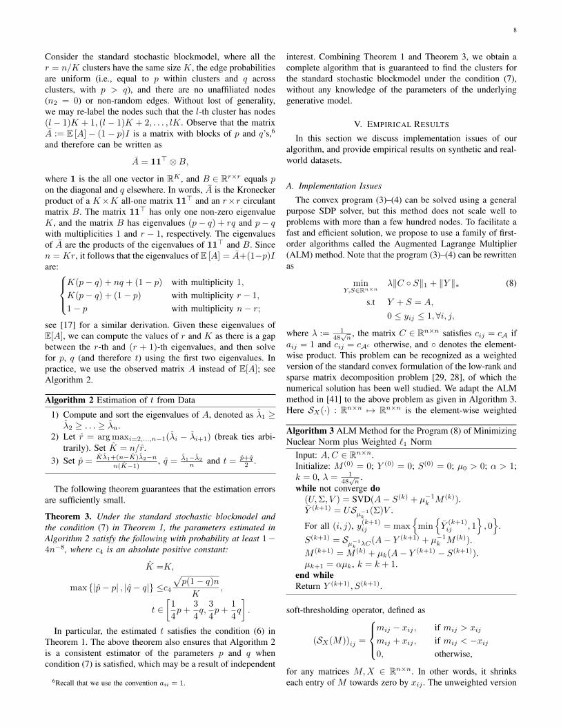
The convex program (3)–(4) can be solved using a generalpurpose SDP solver, but this method does not scale well toproblems with more than a few hundred nodes. To facilitate afast and efficient solution, we propose to use a family of first-order algorithms called the Augmented Lagrange Multiplier(ALM) method. Note that the program (3)–(4) can be rewrittenas

minY,S∈Rn×n

λ‖C S‖1 + ‖Y ‖∗ (8)

s.t Y + S = A,

0 ≤ yij ≤ 1,∀i, j,

where λ := 148√n

, the matrix C ∈ Rn×n satisfies cij = cA ifaij = 1 and cij = cAc otherwise, and denotes the element-wise product. This problem can be recognized as a weightedversion of the standard convex formulation of the low-rank andsparse matrix decomposition problem [29, 28], of which thenumerical solution has been well studied. We adapt the ALMmethod in [41] to the above problem as given in Algorithm 3.Here SX(·) : Rn×n 7→ Rn×n is the element-wise weighted

Algorithm 3 ALM Method for the Program (8) of MinimizingNuclear Norm plus Weighted `1 Norm

Input: A,C ∈ Rn×n.Initialize: M (0) = 0; Y (0) = 0; S(0) = 0; µ0 > 0; α > 1;k = 0, λ = 1

48√n

.while not converge do

(U,Σ, V ) = SVD(A− S(k) + µ−1k M (k)).

Y (k+1) = USµ−1k

(Σ)V .

For all (i, j), y(k+1)ij = max

min

Y

(k+1)ij , 1

, 0

.

S(k+1) = Sµ−1k λC(A− Y (k+1) + µ−1

k M (k)).M (k+1) = M (k) + µk(A− Y (k+1) − S(k+1)).µk+1 = αµk, k = k + 1.

end whileReturn Y (k+1), S(k+1).

soft-thresholding operator, defined as

(SX(M))ij =

mij − xij , if mij > xij

mij + xij , if mij < −xij0, otherwise,

for any matrices M,X ∈ Rn×n. In other words, it shrinkseach entry of M towards zero by xij . The unweighted version

9

0 20 40 60 80 100 120 14010

−6

10−4

10−2

100

102

Iteration

Re

sid

ua

l

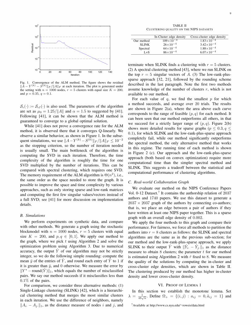
Fig. 1. Convergence of the ALM method. The figure shows the residual‖A− Y (k) − S(k)‖F /‖A‖F at each iteration. The plot is generated underthe setting with n = 1000 nodes, r = 5 clusters with equal size K = 200,and p = 0.35, q = 0.1.

Sε(·) := SεI(·) is also used. The parameters of the algorithmare set as µ0 = 1.25/‖A‖ and α = 1.5 to suggested by [41].Following [41], it can be shown that the ALM method isguaranteed to converge to a global optimal solution.

While [41] does not prove a convergence rate for the ALMmethod, it is observed there that it converges Q-linearly. Weobserve a similar behavior, as shown in Figure 1. In the subse-quent simulations, we use ‖A−Y (k)−S(k)‖F /‖A‖F ≤ 10−2

as the stopping criterion, so the number of iteration neededis usually small. The main bottleneck of the algorithm iscomputing the SVD in each iteration. Therefore, the timecomplexity of the algorithm is roughly the time for oneSVD multiplied by the number of iterations. This can becompared with spectral clustering, which requires one SVD.The memory requirement of the ALM algorithm is Θ(n2), i.e.,the same order as the space needed to store the graph. It ispossible to improve the space and time complexity by variousapproaches, such as only storing sparse and low-rank matricesand computing the first few singular values/vectors instead ofa full SVD; see [41] for more discussion on implementationdetails.

B. Simulations

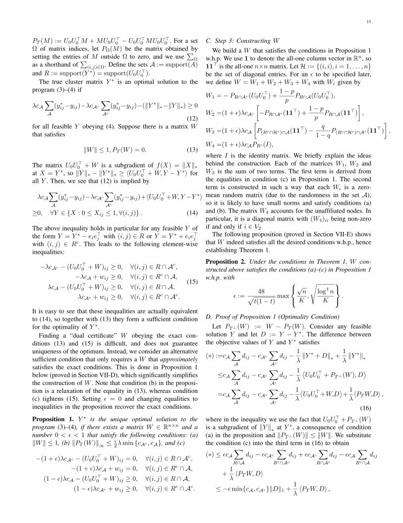
We perform experiments on synthetic data, and comparewith other methods. We generate a graph using the stochasticblockmodel with n = 1000 nodes, r = 5 clusters with equalsize K = 200, and p, q ∈ [0, 1]. We apply our method tothe graph, where we pick t using Algorithm 2 and solve theoptimization problem using Algorithm 3. Due to numericalaccuracy, the output Y of our algorithm may not be strictlyinteger, so we do the following simple rounding: compute themean y of the entries of Y , and round each entry of Y to 1 ifit is greater than y, and 0 otherwise. We measure the error by‖Y ∗− round(Y )‖1, which equals the number of misclassifiedpairs. We say our method succeeds if it misclassifies less than0.1% of the pairs.

For comparison, we consider three alternative methods: (1)Single-Linkage clustering (SLINK) [42], which is a hierarchi-cal clustering method that merges the most similar clustersin each iteration. We use the difference of neighbors, namely‖Ai· − Aj·‖1, as the distance measure of nodes i and j, and

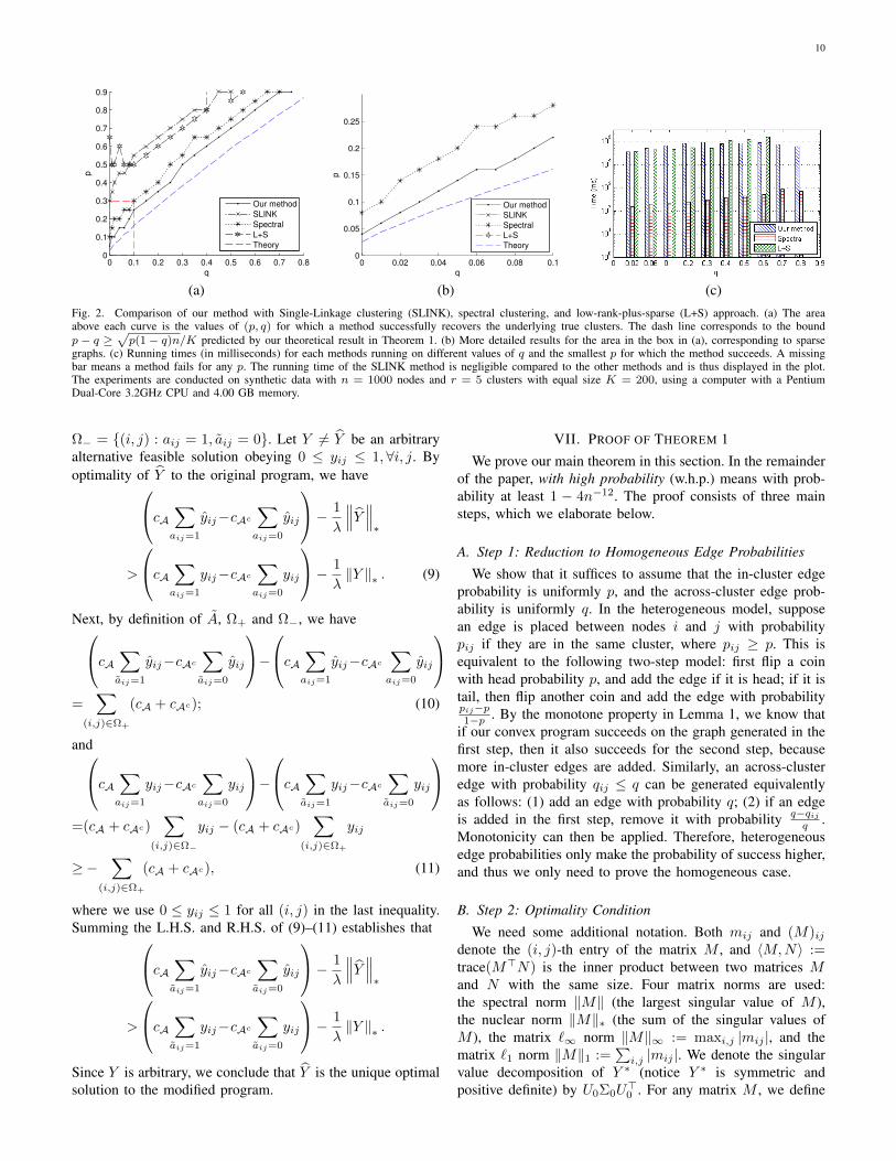
TABLE IICLUSTERING QUALITY ON THE NIPS DATASETS

In-Cluster edge density Cross-cluster edge densityOur method 109×10−4 1.83×10−4

SLINK 26×10−4 3.42×10−4

Spectral 64×10−4 1.88×10−4

L+S 86×10−4 6.07×10−4

terminate when SLINK finds a clustering with r = 5 clusters.(2) A spectral clustering method [43], where we run SLINK onthe top r = 5 singular vectors of A. (3) The low-rank-plus-sparse approach [32, 21], followed by the rounding schemedescribed in the last paragraph. Note the first two methodsassume knowledge of the number of clusters r, which is notavailable to our method.

For each value of q, we find the smallest p for whicha method succeeds, and average over 20 trials. The resultsare shown in Figure 2(a), where the area above each curvecorresponds to the range of feasible (p, q) for each method. Itcan been seen that our method outperforms all others, in thatwe succeed for a strictly larger range of (p, q). Figure 2(b)shows more detailed results for sparse graphs (p ≤ 0.3, q ≤0.1), for which SLINK and the low-rank-plus-sparse approachcompletely fail, while our method significantly outperformsthe spectral method, the only alternative method that worksin this regime. The running time of each method is shownin Figure 2 (c). Our approach and the low-rank-plus-sparseapproach (both based on convex optimization) require morecomputational time than the simpler spectral method andSLINK. This suggests a tradeoff between the statistical andcomputational performance of clustering algorithms.

C. Real-world Collaboration GraphWe evaluate our method on the NIPS Conference Papers

Vol. 0-12 Dataset.7 It contains the authorship relation of 2037authors and 1740 papers. We use this dataset to generate a2037 × 2037 graph of the authors by connecting co-authors;that is, we place an edge between a pair of authors if theyhave written at least one NIPS paper together. This is a sparsegraph with an overall edge density of 0.002.

We apply the four methods to this graph and compare theirperformance. For fairness, we force all methods to partition theauthors into r = 8 clusters as follows: the SLINK and spectralalgorithms are the same as in the previous sub-section; forour method and the low-rank-plus-sparse approach, we applySLINK to their output Y with ‖Yi· − Yj·‖1 as the distancemeasure to obtain 8 clusters; the parameter t for our methodis estimated using Algorithm 2 with r fixed to 8. We measurethe quality of the solutions by computing the in-cluster andcross-cluster edge densities, which are shown in Table II.The clustering produced by our method has higher in-clusterdensity and lower cross-cluster density.

VI. PROOF OF LEMMA 1In this section we establish the monotone lemma. Set

λ = 148√n

. Define Ω+ = (i, j) : aij = 0, aij = 1 and

7Available at http://www.cs.nyu.edu/∼roweis/data.html

10

0 0.1 0.2 0.3 0.4 0.5 0.6 0.7 0.80

0.1

0.2

0.3

0.4

0.5

0.6

0.7

0.8

0.9

q

p

Our method

SLINK

Spectral

L+S

Theory

0 0.02 0.04 0.06 0.08 0.10

0.05

0.1

0.15

0.2

0.25

q

p

Our method

SLINK

Spectral

L+S

Theory

(a) (b) (c)Fig. 2. Comparison of our method with Single-Linkage clustering (SLINK), spectral clustering, and low-rank-plus-sparse (L+S) approach. (a) The areaabove each curve is the values of (p, q) for which a method successfully recovers the underlying true clusters. The dash line corresponds to the boundp− q ≥

√p(1− q)n/K predicted by our theoretical result in Theorem 1. (b) More detailed results for the area in the box in (a), corresponding to sparse

graphs. (c) Running times (in milliseconds) for each methods running on different values of q and the smallest p for which the method succeeds. A missingbar means a method fails for any p. The running time of the SLINK method is negligible compared to the other methods and is thus displayed in the plot.The experiments are conducted on synthetic data with n = 1000 nodes and r = 5 clusters with equal size K = 200, using a computer with a PentiumDual-Core 3.2GHz CPU and 4.00 GB memory.

Ω− = (i, j) : aij = 1, aij = 0. Let Y 6= Y be an arbitraryalternative feasible solution obeying 0 ≤ yij ≤ 1,∀i, j. Byoptimality of Y to the original program, we havecA∑

aij=1

yij−cAc∑aij=0

yij

− 1

λ

∥∥∥Y ∥∥∥∗

>

cA∑aij=1

yij−cAc∑aij=0

yij

− 1

λ‖Y ‖∗ . (9)

Next, by definition of A, Ω+ and Ω−, we havecA∑aij=1

yij−cAc∑aij=0

yij

−cA∑

aij=1

yij−cAc∑aij=0

yij

=

∑(i,j)∈Ω+

(cA + cAc); (10)

andcA∑aij=1

yij−cAc∑aij=0

yij

−cA∑

aij=1

yij−cAc∑aij=0

yij

=(cA + cAc)

∑(i,j)∈Ω−

yij − (cA + cAc)∑

(i,j)∈Ω+

yij

≥−∑

(i,j)∈Ω+

(cA + cAc), (11)

where we use 0 ≤ yij ≤ 1 for all (i, j) in the last inequality.Summing the L.H.S. and R.H.S. of (9)–(11) establishes thatcA∑

aij=1

yij−cAc∑aij=0

yij

− 1

λ

∥∥∥Y ∥∥∥∗

>

cA∑aij=1

yij−cAc∑aij=0

yij

− 1

λ‖Y ‖∗ .

Since Y is arbitrary, we conclude that Y is the unique optimalsolution to the modified program.

VII. PROOF OF THEOREM 1We prove our main theorem in this section. In the remainder

of the paper, with high probability (w.h.p.) means with prob-ability at least 1 − 4n−12. The proof consists of three mainsteps, which we elaborate below.

A. Step 1: Reduction to Homogeneous Edge Probabilities

We show that it suffices to assume that the in-cluster edgeprobability is uniformly p, and the across-cluster edge prob-ability is uniformly q. In the heterogeneous model, supposean edge is placed between nodes i and j with probabilitypij if they are in the same cluster, where pij ≥ p. This isequivalent to the following two-step model: first flip a coinwith head probability p, and add the edge if it is head; if it istail, then flip another coin and add the edge with probabilitypij−p1−p . By the monotone property in Lemma 1, we know that

if our convex program succeeds on the graph generated in thefirst step, then it also succeeds for the second step, becausemore in-cluster edges are added. Similarly, an across-clusteredge with probability qij ≤ q can be generated equivalentlyas follows: (1) add an edge with probability q; (2) if an edgeis added in the first step, remove it with probability q−qij

q .Monotonicity can then be applied. Therefore, heterogeneousedge probabilities only make the probability of success higher,and thus we only need to prove the homogeneous case.

B. Step 2: Optimality Condition

We need some additional notation. Both mij and (M)ijdenote the (i, j)-th entry of the matrix M , and 〈M,N〉 :=trace(M>N) is the inner product between two matrices Mand N with the same size. Four matrix norms are used:the spectral norm ‖M‖ (the largest singular value of M ),the nuclear norm ‖M‖∗ (the sum of the singular values ofM ), the matrix `∞ norm ‖M‖∞ := maxi,j |mij |, and thematrix `1 norm ‖M‖1 :=

∑i,j |mij |. We denote the singular

value decomposition of Y ∗ (notice Y ∗ is symmetric andpositive definite) by U0Σ0U

>0 . For any matrix M , we define

11

PT (M) := U0U>0 M + MU0U

>0 − U0U

>0 MU0U

>0 . For a set

Ω of matrix indices, let PΩ(M) be the matrix obtained bysetting the entries of M outside Ω to zero, and we use

∑Ω

as a shorthand of∑

(i,j)∈Ω. Define the sets A := support(A)

and R := support(Y ∗) = support(U0U>0 ).

The true cluster matrix Y ∗ is an optimal solution to theprogram (3)–(4) if

λcA∑A

(y∗ij−yij)−λcAc∑Ac

(y∗ij−yij)−(‖Y ∗‖∗−‖Y ‖∗) ≥ 0

(12)for all feasible Y obeying (4). Suppose there is a matrix Wthat satisfies

‖W‖ ≤ 1, PT (W ) = 0. (13)

The matrix U0U>0 + W is a subgradient of f(X) = ‖X‖∗

at X = Y ∗, so ‖Y ‖∗ − ‖Y ∗‖∗ ≥ 〈U0U>0 + W,Y − Y ∗〉 for

all Y . Then, we see that (12) is implied by

λcA∑A

(y∗ij−yij)−λcAc∑Ac

(y∗ij−yij)+〈U0U>0 +W,Y −Y ∗〉

≥0, ∀Y ∈ X : 0 ≤ Xij ≤ 1,∀(i, j) . (14)

The above inequality holds in particular for any feasible Y ofthe form Y = Y ∗ − eie>j with (i, j) ∈ R or Y = Y ∗ + eie

>j

with (i, j) ∈ Rc. This leads to the following element-wiseinequalities:

−λcAc − (U0U>0 +W )ij ≥ 0, ∀(i, j) ∈ R ∩ Ac,−λcA + wij ≥ 0, ∀(i, j) ∈ Rc ∩ A,

λcA − (U0U>0 +W )ij ≥ 0, ∀(i, j) ∈ R ∩ A,λcAc + wij ≥ 0, ∀(i, j) ∈ Rc ∩ Ac.

(15)

It is easy to see that these inequalities are actually equivalentto (14), so together with (13) they form a sufficient conditionfor the optimality of Y ∗.

Finding a “dual certificate” W obeying the exact con-ditions (13) and (15) is difficult, and does not guaranteeuniqueness of the optimum. Instead, we consider an alternativesufficient condition that only requires a W that approximatelysatisfies the exact conditions. This is done in Proposition 1below (proved in Section VII-D), which significantly simplifiesthe construction of W . Note that condition (b) in the proposi-tion is a relaxation of the equality in (13), whereas condition(c) tightens (15). Setting ε = 0 and changing equalities toinequalities in the proposition recover the exact conditions.

Proposition 1. Y ∗ is the unique optimal solution to theprogram (3)–(4), if there exists a matrix W ∈ Rn×n and anumber 0 < ε < 1 that satisfy the following conditions: (a)‖W‖ ≤ 1, (b) ‖PT (W )‖∞ ≤

ε2λmin cAc , cA, and (c)

−(1 + ε)λcAc − (U0U>0 +W )ij = 0, ∀(i, j) ∈ R ∩ Ac,

−(1 + ε)λcA + wij = 0, ∀(i, j) ∈ Rc ∩ A,(1− ε)λcA − (U0U

>0 +W )ij ≥ 0, ∀(i, j) ∈ R ∩ A,

(1− ε)λcAc + wij ≥ 0, ∀(i, j) ∈ Rc ∩ Ac.

C. Step 3: Constructing WWe build a W that satisfies the conditions in Proposition 1

w.h.p. We use 1 to denote the all-one column vector in Rn, so11> is the all-one n×n matrix. LetH := (i, i), i = 1, . . . , nbe the set of diagonal entries. For an ε to be specified later,we define W = W1 +W2 +W3 +W4 with Wi given by

W1 =− PR∩Ac(U0U>0 ) +

1− pp

PR∩A(U0U>0 ),

W2 =(1 + ε)λcAc

[−PR∩Ac(11>) +

1− pp

PR∩A(11>)

],

W3 =(1 + ε)λcA

[P(Rc∩Hc)∩A(11>)− q

1− qP(Rc∩Hc)∩Ac(11

>)

],

W4 =(1 + ε)λcAPRc(I),

where I is the identity matrix. We briefly explain the ideasbehind the construction. Each of the matrices W1, W2 andW3 is the sum of two terms. The first term is derived fromthe equalities in condition (c) in Proposition 1. The secondterm is constructed in such a way that each Wi is a zero-mean random matrix (due to the randomness in the set A),so it is likely to have small norms and satisfy conditions (a)and (b). The matrix W4 accounts for the unaffiliated nodes. Inparticular, it is a diagonal matrix with (W4)ii being non-zeroif and only if i ∈ V2

The following proposition (proved in Section VII-E) showsthat W indeed satisfies all the desired conditions w.h.p., henceestablishing Theorem 1.

Proposition 2. Under the conditions in Theorem 1, W con-structed above satisfies the conditions (a)–(c) in Proposition 1w.h.p. with

ε :=48√t(1− t)

max

√n

K,

√log4 n

K

.

D. Proof of Proposition 1 (Optimality Condition)Let PT⊥(W ) := W − PT (W ). Consider any feasible

solution Y and let D := Y − Y ∗. The difference betweenthe objective values of Y and Y ∗ satisfies

(∗) :=cA∑Adij − cAc

∑Ac

dij −1

λ‖Y ∗ +D‖∗ +

1

λ‖Y ∗‖∗

≤cA∑Adij − cAc

∑Ac

dij −1

λ

⟨U0U

>0 + PT⊥(W ), D

⟩=cA

∑Adij − cAc

∑Ac

dij −1

λ

⟨U0U

>0 +W,D

⟩+

1

λ〈PTW,D〉 ,

(16)

where in the inequality we use the fact that U0U>0 +PT⊥(W )

is a subgradient of ‖Y ‖∗ at Y ∗, a consequence of condition(a) in the proposition and ‖PT⊥(W )‖ ≤ ‖W‖. We substitutethe condition (c) into the third term in (16) to obtain

(∗) ≤ εcA∑R∩A

dij − εcAc∑

Rc∩Acdij + εcAc

∑R∩Ac

dij − εcA∑Rc∩A

dij

+1

λ〈PTW,D〉

≤ −εmincA, cAc‖D‖1 +1

λ〈PTW,D〉 ,

12

where we used the fact that dij ≤ 0 for (i, j) ∈ R and dij ≥ 0for (i, j) ∈ Rc since Y = Y ∗ + D satisfies (4). Applyingcondition (b) yields

(∗) ≤ −εmin cAc , cA ‖D‖1 +1

λ‖PTW‖∞ ‖D‖1

≤ − ε2

min cAc , cA ‖D‖1 .

The last R.H.S. is strictly negative whenever D 6= 0. Thisproves that Y ∗ is the unique optimal solution.

E. Proof of Proposition 2

We show that W constructed in Section VII-C satisfies theconditions in Proposition 1 w.h.p. We need two technical lem-mas. First notice that the conditions (6) and (7) in Theorem 1imply bounds on various quantities.

Lemma 2. Under conditions (6) and (7) in Theorem 1, wehave p(1− q) ≥ t(1− t) ≥ cmax

nK2 ,

log4 nK

and ε < 1

2 .

Proof. Since 1 > t > 0, we have t(1− t) ≥ 12 mint, 1− t.

Under condition (6) on t, we further have min t, 1− t ≥14 (p − q) and p(1 − q) ≥ t(1 − t). It then follows fromcondition (7) that

t(1− t) ≥ 1

8(p− q) ≥ c′

√t(1− t) max

√n

K,

√log4 n

K

,

which implies the inequalities in part (1) of the lemma. Part (2)follows directly from part (1) and the definition of ε.

Due to the randomness ofA, W1, W2 and W3 are symmetricrandom matrices with independent zero-mean entries. Thesupport and variance of their entries are bounded in thefollowing lemma.

Lemma 3. The following holds under the GSBM and theconditions (6) and (7) in Theorem 1.

1) For i = 1, 2, 3, the absolute values of the entries of Wi

are bounded by Bi a.s. and their variance is bounded byσ2i , where

B1 :=1

pK, σ2

1 :=1

pK2,

B2 :=2

pλcAc , σ2

2 :=4(1− t)

pλ2c2Ac ,

B3 :=2

1− qλcA, σ2

3 :=4t

1− qλ2c2A.

2) We have σi ≥ cBi log2 n√K

for i = 1, 2, 3.

Proof. The first part of the lemma follows from the definitionsof the Wi’s, q ≤ t ≤ p and ε < 1

2 (Lemma 2). The secondpart follows from Lemma 2.

We now proceed with the proof of Proposition 2, Theproof has three sub-steps, corresponding to checking the threeconditions in Proposition 1.

(1) Bounding ‖W‖.Recall that W1 is a random matrix with i.i.d. entries, and

their absolute values and variance are bounded in Lemma 3.

We apply standard bounds on the spectral norm of randommatrices (Lemma 4 in the Appendix) to obtain w.h.p.

‖W1‖ ≤ 61

K

√1

p

√n ≤ 1

4,

where the last inequality follows from p ≥ c nK2 (cf. Lemma 2).

In a similar manner, we obtain that w.h.p.

‖W2‖ ≤ 6 · 2√

1− tp

λcAc ·√n

= 12

√(1− t)p

· 1

48

√t

(1− t)n·√n ≤ 1

4,

where the last inequality follows from p ≥ t, and w.h.p.

‖W3‖ ≤ 6 · 2√

t

1− qλcA ·

√n

= 12

√t

1− q· 1

48

√1− ttn·√n ≤ 1

4,

where the last inequality follows from 1− t ≤ 1− q. Finally,since W4 = (1 + ε)λcAPRc(I) is a diagonal matrix, we have

‖W4‖ ≤ (1 + ε)λcA ≤ 2 · 1

48

√1− ttn≤ 1

4

since t ≥ c 1n (cf. Lemma 2). We conclude that ‖W‖ ≤∑4

i=1 ‖Wi‖ ≤ 1.(2) Bounding ‖PTW‖∞.Define the sets Rm := (i, j) : i, j in cluster m, and recall

that r is the number of clusters and R := support(Y ∗) =⋃rm=1Rm. We have Y ∗ =

∑rm=1 PRm(11>), and thus its

singular vectors satisfies

U0U>0 =

r∑m=1

1

kmPRm(11>).

Therefore, for i = 1, 2, 3, each entry of the matrix U0U>0 Wi

equals 1km

times the sum of km independent zero-meanrandom variables (which are the entries of Wi), whose absolutevalues and variance are bounded in Lemma 3. Therefore,∥∥U0U

>0 Wi

∥∥∞ can be bounded by applying the standard

Bernstein inequality (given as Lemma 5 in the Appendix) toeach entry of U0U

>0 Wi and then using the union bound over

all the entries. More specifically, by choosing the constant c0in Lemma 5 sufficiently large such that c1 in the same lemmais at least 14, we have the following:

• The matrix W1 satisfies

∥∥U0U>0 W1

∥∥∞ ≤

1

K· c0√

1

pK2

√K log n

= c01

K

√log n

pK≤ log2 n

242

√1

Knw.h.p.,

where we use p ≥ c nK2 in the last inequality (cf.

Lemma 2) with c sufficiently large.

13

• Similarly, the matrix W2 satisfies∥∥U0U>0 W2

∥∥∞ ≤

1

K· c0√

1− tp

λcAc√K log n

=c0

√(1− t) log n

pK

1

48

√t

(1− t)n

≤ log2 n

242

√1

Knw.h.p.,

where we use p ≥ t and log n being sufficiently large inthe last inequality.

• The matrix W3 satisfies∥∥U0U>0 W3

∥∥∞ ≤

1

K· c0√

t

1− qλcA

√K log n

=c0

√t log n

(1− q)K1

48

√1− ttn

≤ log2 n

242

√1

Knw.h.p.,

where we use 1− q ≥ 1− t and log n being sufficientlyin the last inequality.

• Finally, since W4 is a diagonal matrix supported on Rc

and U0U>0 is supported on R, we have U0U

>0 W4 = 0.

On the other hand, we have

λcAε ≥1

48

√1− ttn· 48

√log4 n

Kt(1− t)

=1

t

√log4 n

Kn≥ 1

24

√log4 n

Kn

and

λcAcε ≥1

48

√t

(1− t)n· 48

√log4 n

Kt(1− t)

=1

(1− t)

√log4 n

Kn≥ 1

24

√log4 n

Kn,

which implies

1

24ελmin cA, cAc ≥

log2 n

242

√1

Kn.

Combining with the previous bounds on∥∥U0U

>0 Wi

∥∥∞ for i =

1, 2, 3, 4, we obtain∥∥(U0U

>0 Wi)

∥∥∞ ≤

124ελmin cA, cAc .

Now observe that since W and U0U>0 are both symmetric,

we have WU0U>0 =

(U0U

>0 W

)>. Furthermore, we have∥∥U0U

>0 WU0U

>0

∥∥∞ ≤

∥∥U0U>0 W

∥∥∞max

j

∑i

∣∣∣(U0U>0

)ij

∣∣∣≤∥∥U0U

>0 W

∥∥∞ .

It follows that

‖PTW‖∞=∥∥U0U

>0 W +WU0U

>0 − U0U

>0 WU0U

>0

∥∥∞

≤∥∥U0U

>0 W

∥∥∞ +

∥∥WU0U>0

∥∥∞ +

∥∥U0U>0 WU0U

>0

∥∥∞

≤3∥∥U0U

>0 W

∥∥∞ ≤ 3

4∑i=1

∥∥U0U>0 Wi

∥∥∞ .

Using the bounds on∥∥U0U

>0 Wi

∥∥∞ derived above, we

obtain that ‖PTW‖∞ ≤ 12 · 124ελmin cA, cAc =

12ελmin cA, cAc.

(3) The two equalities in condition (c) in Proposition 1 holdby the definition of W . The two inequalities in condition (c)follow from simple algebra as follows. Because 1− q ≥ 1−t and p ≤ 4t, we have 1−q

p ≥ 14

1−tt . It follows from the

conditions in Theorem 1 that

p− q4≥c√p(1−q) max

√n

K,

√log4 n

K

≥8p(1−t) · 48√

t(1−t)max

√n

K,

√log4 n

K

=8p(1−t)ε.

(17)

We thus have

p− t ≥ p−(

3

4p+

1

4q

)=p− q

4≥ 8p(1− t)ε.

One verifies that this implies (1 + ε)√

t1−t

1−pp ≤ (1 −

2ε)√

1−tt . Plugging in the values of cA and cAc in (5) yields

(1 + ε)cAc(1− p)

p≤ (1− 2ε)cA,

Hence, for each (i, j) ∈ R ∩ A, we have

(U0U>0 +W )ij =

1

p(U0U

>0 )ij + (1 + ε)λcAc

1− pp

≤ 1

p(U0U

>0 )ij + (1− 2ε)cA. (18)

We also have

1

p(U0U

>0 )ij ≤

1

pK

(i)

≤ 48

K

√n

t(1− t)· 1

48

√1− ttn≤ ε · λcA,

(19)

where (i) follows from p ≥ t. Combining (18) and (19) provesthe first inequality in the condition (c).

Similarly, we have

t−q ≥(p

4+

3q

4

)−q =

p− q4

(ii)

≥ 8p(1−t)ε(iii)

≥ 2t(1−q)ε,

where (ii) follows from (17) and (iii) follows from p ≥ tand 1 − t ≥ 1 − 3

4p −14q ≥

14 (1 − q). This implies (1 +

ε)√

1−tt

q1−q ≤ (1 − ε)

√t

1−t . Therefore, for each (i, j) ∈Rc ∩ Ac, we have

wij = −(1 + ε)cAq

1− q≥ −(1− ε)cAc ,

proving the second inequality in condition (c). This completesthe proof of Proposition 2.

14

VIII. PROOF OF THEOREM 2

We use a standard information theoretic argument via Fano’sinequality. For simplicity we assume n1/K and n2/K areboth integers, and we use c1, c2 . . . to denote positive absoluteconstants. Let F be the set of all possible ways of assigningn nodes into n1/K clusters of equal size K. When K =Θ(n1) = Θ(n2), the cardinality of F can be bounded as

M := |F| = 1

(n1/K)!

(n

K

)(n−KK

)· · ·(n1+K

K

)≥ c2·c

12n1

for some c1 > 1 and c2 > 0.Suppose the true cluster matrix Y ∗ is obtained uniformly

at random from F , and the graph A is generated from Y ∗

according to GSBM with uniform edge probabilities. We usePA|Y ∗ to denote the distribution of A given Y ∗. Let Y be anymeasurable function of A. The Fano’s inequality [44] gives

supY ∗∈F

P[Y 6= Y ∗|Y ∗

]≥ 1− I (A;Y ∗) + log 2

logM

≥ 1− I (A;Y ∗) + log 2

c3n

for n is sufficiently large, where I(A;Y ∗) is the mutualinformation between A and Y ∗. We now bound I(A;Y ∗). LetH(·) denote the Shannon entropy and H(·|Y ∗) the Shannonentropy conditioned on Y ∗. Observe that

I(A;Y ∗) =H(A)−H(A|Y ∗) ≤∑

(i,j):i>j

H(aij)−H(A|Y ∗)

=

(n

2

)H(a12)−

(n

2

)H(a12|Y ∗) =

(n

2

)I(a12;Y ∗),

where in the second equality we have used the symmetry underthe uniform distribution of Y ∗ and the conditional indepen-dence between a′ijs. By definition of the mutual information,we have

I(a12;Y ∗) = I(a12; y∗12) = Ey∗12 [D (P(a12|y∗12)‖P(a12))] .

We can directly compute the divergence on the last RHS. Letα := P(y∗12 = 1) = (K−1)n1

n2 and γ := P(a11 = 1) = αp +(1− α)q. It follows that

Ey∗12 [D (P(a12|y12)‖P(a12))]

=αp logp

γ+ α(1− p) log

(1− p)(1− γ)

+ (1− α)q logq

γ

+ (1− α)(1− q) log(1− q)(1− γ)

≤αp(p

γ−1

)+ α(1−p)

(1−p1−γ

−1

)+ (1−α)q

(q

γ−1

)+(1−α)(1−q)

(1−q1−γ

−1

)=α(1− α)(p− q)2

γ(1− γ)≤ c4

(p− q)2

p(1− q),

where in the last inequality we use γ ≥ αp, 1 − γ ≥ (1 −α)(1− q) and α, 1−α = Θ(1). Combining pieces, we obtain

supY ∈F

P[Y 6= Y |Y

]≥ 1−

c5(p−q)2n2

p(1−q) + log 2

c3n.

For the last R.H.S. to be less than 14 , we need (p−q)2

p(1−q) ≥ c61n .

This completes the proof of the theorem.

IX. PROOF OF THEOREM 3

Suppose the eigenvalues of the matrix E[A] are λ1 ≥λ2 ≥ · · · ≥ λn, whose values are computed in Section IV-D.Observe that the matrix A − EA is a random symmetricmatrix with independent zero-mean entries, each of which isbounded in absolute value by 1 and has variance boundedby maxp(1 − p), q(1 − q) ≤ p(1 − q). Under the con-dition of Theorem 3, we may apply Lemma 4 to obtain‖A− EA‖ ≤ 4

√p(1− q)n w.h.p. It then follows from Weyl’s

inequality [45] that w.h.p.

maxi

∣∣∣λi − λi∣∣∣ ≤ ‖A− EA‖ ≤ 4√p(1− q)n. (20)

In the sequel, we assume we are on the event that (20) holds.a) Estimation of r : Recall that λ1 = K(p−q)+nq+(1−

p), λ2, . . . , λr = K(p−q)+(1−p), and λr+1, . . . , λn = 1−p.The inequality (20) implies that for some universal constantc1:

• λ1 − λ2 ≤ λ1 − λ2 +∣∣∣λ1 − λ1

∣∣∣ +∣∣∣λ2 − λ2

∣∣∣ ≤ nq +

c1√p(1− q)n;

• similarly, λi− λi+1 ≤ c1√p(1− q)n for i = 2, . . . r− 1

and i ≥ r + 1;• λr − λr+1 ≥ λr − λr+1 −

∣∣∣λr − λr∣∣∣− ∣∣∣λr+1 − λr+1

∣∣∣ ≥K(p− q)− c1

√p(1− q)n.

Under the condition (7), we have K(p− q) ≥ c2√p(1− q)n

for some constant c2. This implies λr − λr+1 >K(p−q)

2 >

λi − λi+1 for all i > 1 and i 6= r. This guarantees r = r andthus K = K.

b) Estimation of p and q: By (20) and the triangleinequality, the estimation error of q satisfies

|q − q| =

∣∣∣∣∣ λ1 − λ1

n− λ2 − λ2

n

∣∣∣∣∣ ≤ c3√p(1− q)nK

.

Similarly, we have

|p− p| =

∣∣∣∣∣Kλ1 + (n− K)λ2 − nn(K − 1)

− Kλ1 + (n−K)λ2 − nn(K − 1)

∣∣∣∣∣=

∣∣∣∣∣K(λ1 − λ1) + (n−K)(λ2 − λ2)

n(K − 1)

∣∣∣∣∣≤c3

√p(1− q)nK

.

c) Choosing t: Using the above bounds on p and q, weobtain

t =p+ q

2+p− p+ q − q

2≤ p+ q

2+ c4

√p(1− q)nK

≤p+ q

2+p− q

4=

3

4p+

1

4q,

where in the last inequality we use p−q4 ≥ c4

√p(1−q)K , satisfied

under the condition (7). This proves one side of the intervalfor t. The other side is proved in a similar way.

15

X. CONCLUSION

This work is motivated by clustering large-scale networkssuch as modern online social networks, where the graphs areoften highly noisy and have heterogeneous and non-randomstructures. We considered a natural and versatile model,namely the semi-random Generalized Stochastic Blockmodel,for clustered random graphs. This model recovers many clas-sical generative models for graph clustering. We presented aconvex optimization formulation, essentially a convexificationof the maximum likelihood estimator. Our theoretic analysisshows that this method is guaranteed to recover the correctclusters under a wide range of parameters of the problem. Infact, our method order-wise outperforms existing methods inthis setting, in the sense that it succeeds under less restrictiveconditions. Experiment results also validate the effectivenessof the proposed method.

Possible directions for future work include fasteralgorithm implementations, developing effective post-processing/rounding schemes when the obtained solution isnot an exact cluster matrix, and extension to online clusteringsettings (e.g., via incremental stochastic optimization [46]).It is also interesting to extend the algorithms and analysisto more general settings beyond the models in Definitions 1and 2, for example, when the in-cluster and cross-clusterdensities are not bounded uniformly and the clusters haveoverlaps.

APPENDIX

In this section, we record two technical lemmas that areneeded in the proofs of our theoretical results. The firstlemma is a standard bound on the spectral norm of a randomsymmetric matrix.

Lemma 4. Suppose Y is a symmetric n × n matrix, whereYij , 1 ≤ i, j ≤ n are independent random variables, each ofwhich has mean 0 and variance at most σ2 and is boundedin absolute value by B. If σ ≥ c1

B log2 n√n

for some absoluteconstant c1 > 0, then with probability at least 1− n−10,

‖Y ‖ ≤ 4σ√n.

Proof. Except for Y being symmetric, the proof is the sameas that of Theorem 3.1 in [47].

The second lemma is a restatement of the standard Bernsteininequality for the sum of independent random variables.

Lemma 5. Let Y1, . . . , YN be independent random variables,each of which is bounded in absolute value by B a.s. and hasvariance bounded by σ2. For any constant c1 > 0, there existsa constant c0 > 0 independent of σ, B, N and n such thatfor any n ≥ 1, if σ ≥ B

√lognN , then we have∣∣∣∣∣

N∑i=1

Yi − E

[N∑i=1

Yi

]∣∣∣∣∣ ≤ c0σ√N log n

with probability at least 1− 2n−c1 .

REFERENCES

[1] S. Fortunato, “Community detection in graphs,” Phys.Rep., vol. 486, no. 3-5, pp. 75–174, 2010.

[2] J. Leskovec, K. J. Lang, A. Dasgupta, and M. W.Mahoney, “Statistical properties of community structurein large social and information networks,” in Proceedingof the 17th international conference on World Wide Web.ACM, 2008, pp. 695–704.

[3] K. Chaudhuri, F. Chung, and A. Tsiatas, “Spectral clus-tering of graphs with general degrees in the extendedplanted partition model,” in Proceedings of the 25thAnnual Conference on Learning Theory (COLT), 2012.

[4] A. Coja-Oghlan, “Coloring semirandom graphs opti-mally,” Automata, Languages and Programming, pp. 71–100, 2004.

[5] A. Condon and R. Karp, “Algorithms for graph partition-ing on the planted partition model,” Random StructuresAlgorithms, vol. 18, no. 2, pp. 116–140, 2001.

[6] P. Holland, K. Laskey, and S. Leinhardt, “Stochasticblockmodels: Some first steps,” Social Networks, vol. 5,pp. 109–137, 1983.

[7] B. P. W. Ames and S. A. Vavasis, “Convex optimizationfor the planted k-disjoint-clique problem,” MathematicalProgramming, vol. 143, no. 1–2, pp. 299–337, 2014.

[8] N. Alon, M. Krivelevich, and B. Sudakov, “Finding alarge hidden clique in a random graph,” Random Struc-tures Algorithms, vol. 13, no. 3-4, pp. 457–466, 1998.

[9] F. McSherry, “Spectral partitioning of random graphs,” inProceedings of 42nd IEEE Symposium on Foundations ofComputer Science. IEEE, 2001, pp. 529–537.

[10] N. Alon and N. Kahale, “A spectral technique for col-oring random 3-colorable graphs,” SIAM J. Comput.,vol. 26, no. 6, pp. 1733–1748, 1997.

[11] B. Bollobas and A. Scott, “Max cut for random graphswith a planted partition,” Combin. Probab. Comput.,vol. 13, no. 4-5, pp. 451–474, 2004.

[12] U. Feige and J. Kilian, “Heuristics for semirandom graphproblems,” J. Comput. System Sci., vol. 63, no. 4, pp.639–671, 2001.

[13] M. Krivelevich and D. Vilenchik, “Semirandom mod-els as benchmarks for coloring algorithms,” in ThirdWorkshop on Analytic Algorithmics and Combinatorics(ANALCO), 2006, pp. 211–221.

[14] R. Boppana, “Eigenvalues and graph bisection: Anaverage-case analysis,” in 28th Annual Symposium onFoundations of Computer Science. IEEE, 1987, pp. 280–285.

[15] M. Jerrum and G. Sorkin, “The metropolis algorithm forgraph bisection,” Discrete Appl. Math., vol. 82, no. 1-3,pp. 155–175, 1998.

[16] T. Carson and R. Impagliazzo, “Hill-climbing finds ran-dom planted bisections,” in Proceedings of the 12thAnnual ACM-SIAM Symposium on Discrete algorithms.SIAM, 2001, pp. 903–909.

[17] J. Giesen and D. Mitsche, “Reconstructing many par-titions using spectral techniques,” in Fundamentals ofComputation Theory. Springer, 2005, pp. 433–444.

16

[18] R. Shamir and D. Tsur, “Improved algorithms for therandom cluster graph model,” Random Structures Algo-rithms, vol. 31, no. 4, pp. 418–449, 2007.

[19] A. Coja-Oghlan, “Graph partitioning via adaptive spec-tral techniques,” Combin. Probab. Comput., vol. 19,no. 2, p. 227, 2010.

[20] K. Rohe, S. Chatterjee, and B. Yu, “Spectral clusteringand the high-dimensional stochastic blockmodel,” Ann.Statist., vol. 39, no. 4, pp. 1878–1915, 2011.

[21] S. Oymak and B. Hassibi, “Finding dense clusters via“Low Rank + Sparse” decomposition,” Arxiv preprintarXiv:1104.5186, 2011.

[22] B. P. W. Ames, “Guaranteed clustering and biclusteringvia semidefinite programming,” Mathematical Program-ming, vol. 147, no. 1–2, pp. 429–465, 2014.

[23] Y. Chen, S. Sanghavi, and H. Xu, “Clustering sparsegraphs,” in Advances in Neural Information ProcessingSystems 25 (NIPS), 2012.

[24] A. Anandkumar, R. Ge, D. Hsu, and S. M. Kakade, “Atensor approach to learning mixed membership commu-nity models,” Journal of Machine Learning Research,vol. 15, pp. 2239–2312, 2014.

[25] N. Ailon, Y. Chen, and H. Xu, “Breaking the smallcluster barrier of graph clustering,” in Proceedings ofthe 30th International Conference on Machine Learning,2013, pp. 995–1003.

[26] A. Decelle, F. Krzakala, C. Moore, and L. Zdeborova,“Asymptotic analysis of the stochastic block model formodular networks and its algorithmic applications,” Phys.Rev. E, vol. 84, no. 6, p. 066106, 2011.

[27] R. R. Nadakuditi and M. Newman, “Graph spectra andthe detectability of community structure in networks,”Phys. Rev. Lett., vol. 108, no. 18, p. 188701, 2012.

[28] V. Chandrasekaran, S. Sanghavi, P. Parrilo, and A. Will-sky, “Rank-sparsity incoherence for matrix decomposi-tion,” SIAM J. Optim., vol. 21, no. 2, pp. 572–596, 2011.

[29] E. J. Candes, X. Li, Y. Ma, and J. Wright, “Robustprincipal component analysis?” J. ACM, vol. 58, no. 3,p. 11, 2011.

[30] Y. Chen, A. Jalali, S. Sanghavi, and C. Caramanis, “Low-rank matrix recovery from errors and erasures,” IEEETrans. Inform. Theory, vol. 59, no. 7, pp. 4324–4337,2013.

[31] X. Li, “Compressed sensing and matrix completion withconstant proportion of corruptions,” Constr. Approx.,vol. 37, no. 1, pp. 73–99, 2013.

[32] Y. Chen, A. Jalali, S. Sanghavi, and H. Xu, “Clusteringpartially observed graphs via convex optimization,” Jour-nal of Machine Learning Research, vol. 15, pp. 2213–2238, June 2014.

[33] B. Recht, M. Fazel, and P. Parrilo, “GuaranteedMinimum-Rank Solutions of Linear Matrix Equations viaNuclear Norm Minimization,” SIAM Rev., vol. 52, no.471, 2010.

[34] C. Mathieu and W. Schudy, “Correlation clustering withnoisy input,” in Proceedings of the Twenty-First AnnualACM-SIAM Symposium on Discrete Algorithms. SIAM,2010, pp. 712–728.

[35] A. Frieze and C. McDiarmid, “Algorithmic theory ofrandom graphs,” Random Structures Algorithms, vol. 10,no. 1-2, pp. 5–42, 1997.

[36] M. R. Garey and D. S. Johnson, Computers and In-tractability: A Guide to the Theory of NP-Completeness.San Francisco, CA: W. H. Freeman, 1979.

[37] U. Feige and E. Ofek, “Spectral techniques appliedto sparse random graphs,” Random Structures & Algo-rithms, vol. 27, no. 2, pp. 251–275, 2005.

[38] E. Hazan and R. Krauthgamer, “How hard is it to ap-proximate the best nash equilibrium?” SIAM J. Comput.,vol. 40, no. 1, pp. 79–91, 2011.

[39] A. Juels and M. Peinado, “Hiding cliques for crypto-graphic security,” Des. Codes Cryptogr., vol. 20, no. 3,pp. 269–280, 2000.

[40] O. Shamir and N. Tishby, “Spectral Clustering on a Bud-get,” in Proceedings of the 14th International Conferenceon Artificial Intelligence and Statistics, Apr. 2011, pp.661–669.

[41] Z. Lin, M. Chen, L. Wu, and Y. Ma, “The AugmentedLagrange Multiplier Method for Exact Recovery of Cor-rupted Low-Rank Matrices,” UIUC Technical ReportUILU-ENG-09-2215, 2009.

[42] R. Sibson, “Slink: an optimally efficient algorithm forthe single-link cluster method,” The Computer Journal,vol. 16, no. 1, pp. 30–34, 1973.

[43] U. Von Luxburg, “A tutorial on spectral clustering,” Stat.Comput., vol. 17, no. 4, pp. 395–416, 2007.

[44] T. M. Cover and J. A. Thomas, Elements of informationtheory, 2nd ed. Wiley, 2006.

[45] R. Bhatia, Perturbation bounds for matrix eigenvalues.Longman, Harlow, 1987.

[46] J. Feng, H. Xu, and S. Yan, “Online robust pca viastochastic optimization,” in Advances in Neural Infor-mation Processing Systems, 2013, pp. 404–412.

[47] D. Achlioptas and F. Mcsherry, “Fast computation oflow-rank matrix approximations,” J. ACM, vol. 54, no. 2,p. 9, 2007.