Improved Efficiency of Glaucoma Detection by using Wavelet ...

1 Nataraj A. Vijapur, Smita M. Chitnis, Dr. R. Srinivasa Rao Kunte

International Journal of Electronics, Electrical and Computational System

IJEECS

ISSN 2348-117X

Volume 3, Issue 8

October 2014

Improved Efficiency of Glaucoma Detection by using Wavelet

Filters, Prediction and Segmentation Method

Nataraj A. Vijapur

Associate Professor, Department of Electronics and Communication, KLEsMSSCET, Belgaum,

India

Smita M. Chitnis

PG Student, Department of Electronics and Communication, KLEsMSSCET, Belgaum, India

Dr. R. Srinivasa Rao Kunte

Professor and Principal, Jawaharlal Nehru National College Of Engineering, Shivamogga, India

Abstract—Glaucoma is the second leading cause of peripheral blindness worldwide and it results in

the neuro-degeneration of the optic nerve. In this paper, the work is focused on improving the

sensitivity of automated classification system for Glaucoma by implementing the two techniques by

extracting image features from eye fundus photographs. A data-driven approach is developed which

requires no manual supervision. Our goal is to establish a screening system that allows fast, and

automated detection of Glaucomatous changes in the eye fundus. Here the work is focused on

extracting the energy features extracted from eye fundus images using Discrete Wavelet Transforms

and segmentation of optic cup and disc. The wavelet features are obtained from the daubechies

(db3), symlets (sym3), and biorthogonal (bio3.3, bio3.5, and bio3.7) wavelet filters. This energy

features obtained from the detailed coefficients can be used to distinguish between normal and

glaucomatous eye images. Along with this technique Optic cup to disc ratio is also calculated, which

improves the accuracy of detecting the Glaucoma. Here optic disc is extracted using disc prediction

method and optic cup is segmented using watershed segmentation. System was tested on the samples

obtained from K.L.E.Dr.Prabhakar Kore Hospital and Medical Research Center, Belgaum,India and

efficiency was found out to be 96%.

Index Terms— Glaucoma, Optic cup, Disc, 2D Wavelet filters of discrete wavelet transform, Pixel

based segmentation, Watershed segmentation.

1. INTRODUCTION

Glaucoma is an eye disease caused by elevated Intra-Ocular Pressure (IOP), which is introduced by

the aqueous humor secreted in the eye. The aqueous humor provides oxygen and vital nutrients to

cornea and lens. It is drained out through the drainage canals of the eye. Glaucoma is developed

when the drainage canals become blocked. Due to this, the aqueous humor cannot drain away

normally and the pressure inside increases. This elevated pressure destroys the optic nerve. Impact of

early stage Glaucoma on vision is as shown in Figure.1.1 and Figure. 1.2. Glaucoma causes

enlargement of optic cup and loss of vision. Enlargement of optic cup is as shown in Fig.2.1 and Fig.

2.2. If the ratio of Optic cup to disc becomes greater than 0.3 it is detected as Glaucoma. It is

important to detect malign changes and abnormal structures of the optic disc as early as possible and



IJEECS

ISSN 2348-117X

Volume 3, Issue 8

October 2014

monitor their progress during clinical therapy. As the revitalization of the degenerated optic nerve

fibers is not viable medically, Glaucoma often goes undetected in its patients until later stages.

Furthermore, in countries, like India, it is estimated that approximately 11.2 million people over the

age of 40 suffer from Glaucoma [1]. It is believed that these numbers can be curtailed with effective

detection and treatment options.

Figure 1.1 Figure 1.2

Normal vision Vision affected by Glaucoma

Usually Retinal image analysis techniques rely on computational techniques to make qualitative

assessments of the eye more reproducible and objective. The goal of using such methods is to reduce

the variability that may arise between different clinicians tracking the progression of structural

characteristics in the eye. Commonly categorized structural features to detect Glaucoma include disc

area, disc diameter, rim area, cup area, cup diameter, cup-to-disc ratio, and topological features

extracted from the image. Proper orthogonal decomposition (POD) is an example of a technique that

uses structural features to identify glaucomatous progression.

Fig.2.1 Fig.2.2

Fundus image of healthy eye Fundus image of Glaucoma affected

eye with showing the Optic Disc and Cup areas enlarged Optic Disc.

2. Objective of the Work

The intent of this work is to improve the accuracy of the Glaucoma detection by calculating the

energy features and optic cup to disc ratio(CDR). To this endeavour, two techniques are used to

detect the progression of Glaucoma.

The energy signatures are obtained by using 2-D Discrete Wavelet Transform and the energy

obtained from the detailed coefficients can be used to distinguish between normal and

glaucomatous eye images. The energy features extracted by using wavelet filters. This data can be

used by the physicians and may help in better understanding of Glaucoma.

The segmentation methods are used to extract the optic cup and optic disc boundaries to calculate

the CDR. The pixel based segmentation is used for optic disc extraction and watershed

segmentation is used for optic cup extraction.

http://www.protect-your-eyesight.com/glaucoma-information.html

http://www.protect-your-eyesight.com/glaucoma.html



IJEECS

ISSN 2348-117X

Volume 3, Issue 8

October 2014

3. Methodology

3.1 Methodology for glaucoma detection by extracting the energy features using 2d

wavelets:

In the proposed method the features are extracted using wavelet filters. Here the input image of a

person is captured by fundus camera. Image is decomposed by using wavelet filters. Extracted

features are fed to SVM classifier. Depending upon the dataset, The classifier classifies the image as

either Glaucoma or Non-Glaucomateous.The proposed method of detecting Glaucoma is as shown in

Fig. 3.1 below.

Figure 3.1: Block diagram of Classification of Glaucoma and Normal Retinal Images.

3.1.1 Discrete wavelet transform – Based energy features

Most of the signals in practice are time-domain signals in their raw format. That is, whatever that

signal is measuring, is a function of time. In other words, when we plot the signal one of the axes is

time (independent variable), and the other (dependent variable) is usually the amplitude. When we

plot time-domain signals, we obtain a time-amplitude representation of the signal. This

representation is not always the best representation of the signal for most signal processing related

applications. In many cases, the most distinguished information is hidden in the frequency content of

the signal.

The wavelet transform (WT) has gained widespread acceptance in signal processing and image

compression. Because of their inherent multi-resolution nature, wavelet-coding schemes are

especially suitable for applications where scalability and tolerable degradation are important.

Wavelet transform decomposes a signal into a set of basis functions. These basis functions are called

wavelets.

In the proposed method three different wavelet filters such as daubechies (db3), symlets (sym3)

and biorthogonal (bio3.3, bio3.5, bio3.7) [3] are used on a set of fundus images by employing 2-D

DWT. The texture features using wavelet transforms in image processing are often employed to

overcome the generalization of features. We calculate the averages of the detailed horizontal and

vertical coefficients and wavelet energy signatures obtained by wavelet decomposition. With the

help of these filters the obtained wavelet coefficients are then subjected to average and energy

calculation resulting in feature extraction. Table 1 shows the obtained features normal range for

Glaucoma detection. Based on the average and energy calculations the images are classified either as

Normal and Glaucoma.

Eye

Fundus Image

Image

Decomposition

Feature Extraction

SVM Classifier

Normal Glaucoma



IJEECS

ISSN 2348-117X

Volume 3, Issue 8

October 2014

TABLE I. WAVELET ENERGY FEATURES FOR GLAUCOMA DETECTION

Features Normal

Db3:

dh1_Average

0.0010 to 0.0017

Db3: cv1_Energy 6.9764e-05to

1.8267e-04

Sym3:

dh1_Average

0.0010 to 0.0017

Sym3:

cv1_Energy

6.9764e-05to

1.8267e-04

Rbio3.3:

dh1_Average

0.0018 to 0.0036

Rbio3.3:

cv1_Energy

1.7000e-04to

4.7205e-04

Rbio3.3:

cd1_Energy

5.8229e-05to

1.5435e-04

Rbio3.5:

dh1_Average

0.0016 to 0.0033

Rbio3.5:

cv1_Energy

1.4163e-04to

3.9048e-04

Rbio3.5:

cd1_Energy

3.8834e-05to

9.9975e-05

Rbio3.7:

dh1_Average

0.0014 to 0.0032

Rbio3.7:

cv1_Energy

1.3235e-04to

3.6286e-04

Feature extraction involves simplifying the amount of resources required to describe a large set of

data accurately. When performing analysis of complex data one of the major problems stems from

the number of variables involved. Analysis with a large number of variables generally requires a

large amount of memory and computation power or a classification algorithm which over fits the

training. Feature extraction is a general term which depicts to extract only valuable information from

given raw data. The main objective of feature extraction is to represent raw image in its reduced form

and also to reduce the original dataset by measuring certain properties to make decision process

easier. A feature is nothing but the significant representative of an image which can be used for

detection of Glaucoma. The extracted features provide characteristics of input pixel [4].The spatial

features can be extracted by statistical and co-occurrence methods.

It is a well-known fact that Fourier Transforms (FT) can be useful for extracting frequency

contents of a stationary signal. However, it cannot provide time-evolving effects of frequencies in

non-stationary signals. STFT suffers from the limitation that it employs a fixed width of window



IJEECS

ISSN 2348-117X

Volume 3, Issue 8

October 2014

function, chosen a priori, and hence it creates a problem for simultaneous analysis of high frequency

and low frequency non-stationary signals.

Hence, wavelet transform arose as an effective tool for those situations where one needs

multiresolution analysis, providing short windows at high frequencies and long windows at low

frequencies. Here each image is represented as a p × q gray-scale matrix I [i,j]. The resultant 2-

DDWTcoefficients are the same irrespective of whether the matrix is traversed top-to-bottom or

bottom-to-top. Hence, it is sufficient that we consider four decomposition directions corresponding

to 0◦ (horizontal, Dh), 45◦ (diagonal, Dd), 90◦ (vertical, Dv), and 135◦ (diagonal, Dd) orientations.

The decomposition structure for one level is illustrated in Figure 3.4. In this figure, I is the image,

g[n] and h[n] are the low-pass and high-pass filters, respectively, and A is the approximation

coefficient. Where, 2ds1 indicates that rows are down sampled by two and columns by one. 1ds2

indicates that rows are down sampled by one and columns by two. The “×” operator indicates

convolution operation. Since the number of elements in these matrices is high, and since we only

need a single number as a representative feature, we employed averaging methods to determine such

single valued features. These are obtained by the following equations,

(1)

(2)

(3)

Energy signatures provide a good indication of the total energy contained at specific spatial

frequency levels and orientations [5].The energy-based approach assumes that different texture

patterns have different energy distribution in the space-frequency domain. The energy obtained from

the detailed coefficients can be used to distinguish between normal and glaucomatous images with

very high accuracy. Hence these energy features are highly discriminatory. This approach is very

appealing due to its low computational complexity involving mainly the calculation of first and

second order moments of transform coefficients.

Image

Figure 3.2: Discrete Wavelet Transform decomposition.

Rows x Rows x

2ds1 2ds1

Columns x g

(n)

Columns x

h (n)

Columns x

g (n)

Columns x h

(n)

1ds2 1ds2

1ds2

1ds2

A1 Dh Dv Dd



IJEECS

ISSN 2348-117X

Volume 3, Issue 8

October 2014

The energy features are fed into classifier Support Vector Machine (SVM) resulting in high

accuracy of classification. The energy features are used to train the Support Vector Machine

classifier which classifies each row of the data in the sample using the information from the classifier

structure SVMStruct. This classifier is trained using a svmtrain and distinguishes the retinal images

into normal or abnormal using the confusion matrix and thereby achieve a high a level of accuracy.

3.2 Methodology for Glaucoma detection using CDR technique:

Glaucoma can also be detected by segmenting the optic cup and optic disc. Here the input image

of a person is captured by fundus camera. Then the captured image is subjected to various pre

processing steps like gray level transformation and enhancement. The noise in the image is filtered

using a mean filter. The optic disc is segmented using disc approximation method based

approach.The optic Cup is segmented by using Watershed transformation. Then the area of the optic

Disc and Cup are measured to calculate CDR. Depending on the value of CDR the fundus image is

classified as Normal or Glaucomatous image. The proposed method of detecting Glaucoma is as

shown in Fig. 3.3 below.

Figure 3.3 Block Diagram of CDR method

3.2.1 Optic Disc Segmentation

To start with the input image is read and converted to gray image (fig 3.4(b)). Filtering of the gray

image is done to improve the quality of the image such as the multidimensional filter for optic Disc

segmentation. The morphological dilation operation is used to perform the addition of image pixels

of highest intensity for making bright accurate circular shape of optic Disc. The following figures

show the sequence of the operations performed on an input colour retinal image.

Fig 3.4: (a) Color fundus input image (b) Gray image (c) Filtered image (d) Dilated image.

3.2.1.1 Filtering Process:

Let Sxy represents the set of coordinates in a rectangular sub image window of size m × n centered at

point (x, y). The arithmetic mean filtering process computes the average value of the corrupted

Eye Fundus

Image Image Pre-

processing

Optic Disc

Segmentation

Optic Cup

Segmentation

Normal

Glaucoma

CDR

Calculator



IJEECS

ISSN 2348-117X

Volume 3, Issue 8

October 2014

image g(x, y) in the area defined by Sxy. The value of the restored image f at any point (x, y) is

simply the arithmetic mean computed using the pixels in the region defined by Sxy. In other words,

This operation can be implemented using a convolution mask in which all coefficients have value

1/mn. A mean filter simply smoothes local variations in an image. Noise is reduced as a result of

blurring. The best known order-statistics filter is the median filter, which replaces the value of an

image pixel by the median of the gray levels in the neighbourhood of that image pixel.

For optic Disc the gray image is filtered by using this multidimensional filter as shown in fig 3.2(c).

Assume that f (x, y) is a gray-scale image and b(x, y) is a structuring element and both functions are

discrete. Similarly to binary morphology, the structuring elements are used to examine a given image

for specific properties.

Intensity threshold for segmentation

The point based or pixel based segmentation is conceptually the simplest approach used for image

segmentation. The pixel values greater than or equal to the threshold value is written as 1’s and

determined that the (threshold) gray levels are assumed to belong to that image, and the pixel values

below that the threshold values are written as 0’s and are assumed to be outside of that image. Here

Fixed thresholding is of the form:

That is the pixels equal or above the threshold value are set to 1’s and otherwise set to 0’s.

3.2.1.2 Dilation process

The dilation of f by a flat structuring element b at any location (x, y) is defined as the maximum value

of the image in the window outlined by when the origin of is at (x, y). Therefore, the dilation at

(x, y) of an image f by a structuring element b is given by:

Where we used that , similarly to the correlation, x and y are decremented through

all values required so that the origin of b visits every pixel in f. That is, to find the dilation of f by b,

we place the origin of the structuring element at every pixel location in the image. The dilation is the

maximum value of f from all values of f in the region of f coincident with b and that the structuring

element is reflected about the origin. The morphological operations are used to simplify image data,

preserve essential shape characteristics and eliminate noise. In the proposed method dilation

morphological operation is used to perform the addition of image pixels of highest intensity for

making bright accurate circular shape of optic Disc. Dilation results, the output of an image are

brighter than the input image and expanded an image to the closest picture of neighbourhood pixel

values. The area of the circular (or elliptical) optic Disc is calculated by counting the number of

intensity of the bright pixels from the morphological gray images as shown in fig 3.2(d).

First step to segment the optic Disc is determination of the center of optic Disc which is the lighter

and brightest part in retinal image. The center of the optic Disc is calculated by traversing through

left and right of the x-axis and up and down of the y-axis of the binary image of extracted Disc. After

determination of the center we have to calculate the radius of optic Disc, this will be done by

exploring and counting the intensity of each pixel from the center of optic Disc (in four direction;



IJEECS

ISSN 2348-117X

Volume 3, Issue 8

October 2014

two horizontally and the other two vertically) toward the optic Disc edges. Determination of the

radiuses in four directions helps to predict the actual radius. When we determine the center and

radius we redraw the optic Disc. Thus the optic Disc is extracted.

Area of the optic Disc is calculated by counting the number of pixels within the optic Disc region.

This area information of the optic Disc is used to find the optic Cup to optic Disc ratio. Figure 3.4(e)

shows the segmented optic Disc area from the input color fundus images which is calculated by

above disc prediction method.

Fig 3.4(e): Segmented Optic Disc

3.2.2. Optic Cup segmentation

To start with the image is filtered and watershed transformation is applied to locate the optic Cup

boundaries. Since the optic Cup represents a bright area, and as blood vessels emerge dark in gray

level retinal images, the gray level variation within the optic Cup region is very high. This variation

is first removed using a closing morphological operation to facilitate later watershed operation.

Particularly, we show how the watershed transformation contributes to improve the numerical

results for optic Cup segmentation problems. Let f(x, y) with (x, y) R2, be a scalar function

describing an image I. The morphological gradient of I is defined by

Where and are respectively the elementary dilation and erosion of f by the

structuring element b. The morphological Laplacian is given by

We note here that this morphological Laplacian allows us to distinguish influence zones of minima

and suprema: regions with GL < 0 are considered as influence zones of suprema, while regions with

GL > 0 are influence zones of minima. Then GL = 0 allows us to interpret edge locations, and will

represent an essential property for the construction of morphological filters. The basic idea is to

apply either dilation or erosion to the image I, depending on whether the pixel is located within the

influence zone of a minimum or a maximum.

If we view an image as a surface, with mountains (high intensity) and valleys (low intensity),

the watershed transform finds intensity valleys in an image. Fig. 3.5 illustrates this approach. We

have considered the same original image as previously. Fig. 3.5.(a) shows the watershed of the image

and Fig. 3.5.(b) shows the watershed of its gradient and Fig 3.5.(c) shows the segmentation results of

the filtered image and finally Fig 3.5(d) shows the optic Cup segmented image.



IJEECS

ISSN 2348-117X

Volume 3, Issue 8

October 2014

(a) (b) (c) (d)

Fig 3.5 (a) watershed of the original image (b) the watershed of its gradient, (c) segmentation

results of the filtered image and finally (d) optic Cup marked image.

As a first step, we eliminate large gray level variations within the papillary region by filtering

the image using morphological closing operator. The removal of large peaks involves opening

operator with large structuring element which alters the shape of the papillary region. So calculate

the morphological reconstruction by dilation. Before we apply the watershed transformation to the

morphological gradient, we impose internal and external markers. We use the locus of optic Cup, f(x,

y) as an internal marker that has been calculated and a square containing the optic Cup with center at

(x, y) as an external marker.

The Catchment basin C (M) associated to a minimum M is the set of pixels of p such that a

water drop falling at p flows down along the relief, following a certain descending path, and

eventually reaches M. The catchment basins of an image I correspond then to the influence zones of

its minima, and the watershed will be defined by the lines that separate adjacent catchment basins.

we consider and the smallest and the largest values taken by f. Let = {p f

(p) ≤ k} be the threshold set of f at level k. We define a recursion with the gray level k increasing

from to , in which the basins associated with the minimum of f are successively expanded.

We consider the union of the set of basins computed at level k. A connected component of the

threshold set Tk+1 at level k+1 can be either a new minimum, or an extension of a basin in .

Finally, by denoting by mink the union of all regional minima at level k, we obtain the following

recursion which defines the watershed by immersion.

With

Where k is the number of minima of I and is defined by

The set of the catchment basins of a gray level image I is equal to the set . At the end of this

process, the watershed of the image I is the complement of in .

Watershed segmentation of the imposed minima image is accomplished with the watershed

function. The watershed function returns a label matrix containing nonnegative numbers that

corresponds to watershed regions. Pixels that do not fall into any watershed region are given a pixel

value of 0. This technique modifies a gray-scale image so that regional minima occur only in marked

locations. Other pixel values are pushed up as necessary to remove all other regional minima. Thus



IJEECS

ISSN 2348-117X

Volume 3, Issue 8

October 2014

the optic Cup is segmented by mathematical morphology and watershed transform. The extracted

optic Cup by watershed transformation method is as shown in fig 3.5(e).

Fig 3.5(e): Segmentation result of optic Cup.

3.2.3 Calculation of CDR

The area of optic cup and optic disc is calculated by counting the number of pixels present in the

optic disc and optic cup respectively. Then the ratio of optic cup to optic disc is calculated. If the

optic cup to optic disc ratio exceeds 0.3 then the image is classified as Glaucoma or else it is

classifies as Normal.

4. Experimental Results

The following section provides a detailed description of the results obtained from feature selection

and classification.

4.1. Results of wavelet based energy features

Figure 4.1 shows the resulting retinal image obtained after converting an color input retinal image

to gray image. Figure4.1 (a) shows the input image and (b) shows the gray scale image.

Figure 4.1 (a) Retinal input image (b) Gray scale image

The energy-based approach assumes that different texture patterns have different energy distribution

in the space-frequency domain. This approach is very appealing due to its low computational

complexity involving mainly the calculation of first and second order moments of transform

coefficients. Figure 4.2 provides a snapshot of the results obtained from Feature extraction described

in the methodology section.

Figure 4.2: Output of daubechies (db3), the symlets (sym3), and the biorthogonal (bio3.3,

bio3.5, and bio3.7) wavelet filters



IJEECS

ISSN 2348-117X

Volume 3, Issue 8

October 2014

Figure above shows the results obtained from daubechies (db3), the symlets (sym3), and the

biorthogonal (bio3.3, bio3.5, and bio3.7) wavelet filters. The horizontal and vertical coefficients of

wavelet filters are used to extract energy features. The different texture patterns have different

energy distribution in the space-frequency domain.

The energy features are extracted for all sample input retinal images. Thus for normal images the

range is being calculated by using the equations 1, 2, 3. We calculate the averages of the detailed

horizontal and vertical coefficients and wavelet energy signature from the detailed vertical

coefficients for daubechies (db3), the symlets (sym3), and the biorthogonal (bio3.3, bio3.5, and

bio3.7) wavelet filters. If the input retinal image energy features are within the range of threshold

value then the image is classified as normal otherwise it is glaucomatous eye.

Figure 4.3: Result of wavelet transform energy features method.

The extracted features were used for Classification [3].The accuracy of the system is calculated.

Figure 4.4: SVM Classifier output

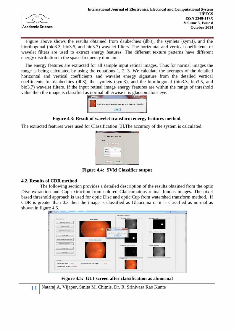
4.2. Results of CDR method

The following section provides a detailed description of the results obtained from the optic

Disc extraction and Cup extraction from colored Glaucomatous retinal fundus images. The pixel

based threshold approach is used for optic Disc and optic Cup from watershed transform method. If

CDR is greater than 0.3 then the image is classified as Glaucoma or it is classified as normal as

shown in figure 4.5.

Figure 4.5: GUI screen after classification as abnormal



IJEECS

ISSN 2348-117X

Volume 3, Issue 8

October 2014

The efficiency of classifier designed was found to be 96% when tested on the samples

obtained from K.L.E.Dr.Prabhakar Kore Hospital and Medical Research Center, Belgaum,India. This

is inclusive of the Methodology for Glaucoma detection by extracting the energy features using 2D

wavelets and CDR technique.

Conclusion

In the proposed method, the Glaucoma is detected by finding the energy features from discrete

wavelet transform and through the measurement of CDR. These two methods together make the

system more reliable in detecting the Glaucoma. The efficiency of classifier designed was found to

be 96%

Here a wavelet-based texture feature set has been used to detect the Glaucoma. The texture feature

set can be enhanced in accuracy by making use of more number of test images. The optic disc has

been segmented based on the principle of disc prediction method. The optic cup has been segmented

based on the watershed transformation. Then the cup-disc ratio is calculated to find the progression

of Glaucoma. Further for both the methodologies test images can be used to decide the threshold

value and improve the accuracy of the system.

Acknowledgments

We would like to express our sincere gratitude to Ophthalmology department K. L. E. Society’s

Dr.Prabhakar Kore Hospital & M.R.C., Belgaum, India for providing us with necessary guidance and

resources required for experimentation. Special thanks to High Resolution Fundus (HRF) Image

Database available on intenet,provided by the Pattern Recognition Lab (CS5), the Department of

Ophthalmology, Friedrich-Alexander University Erlangen-Nuremberg (Germany), and the Brno

University of Technology, Faculty of Electrical Engineering and Communication, Department of

Biomedical Engineering, Brno (Czech Republic). We would like to thank Research Center, E & C

department of Jawaharlal Nehru National College of Engineering, Shivamogga, India for technical

guidance and resources without which venture would not have been possible.

References

[1] Nataraj A.Vijapur, Dr. R. Srinivasa Rao Kunte, Dr.Rekha Mudhol, ”An Approach For Detection

Of Primary Open Angle Glaucoma”. International Journal of Advanced Research in Engineering

and Technology (IJARET), Volume 4, Issue 6, pp. 185-194, 2013.

[2] R. George, R. S. Ve, and L. Vijaya, “Glaucoma in India: Estimated burden of disease,” J.

Glaucoma, vol. 19, pp. 391–397, Aug. 2010.

[3] K. R. Sung et al., “Imaging of the retinal nerve fiber layer with spectral domain optical coherence tomography for glaucoma diagnosis,” Br. J. Ophthalmol., 2010.

[4] Sumeet Dua,U. Rajendra Acharya, Pradeep Chowriappaand S. Vinitha Sree, “Wavelet-Based

Energy Features for Glaucomatous Image Classification ”,Vol. 16, no.1,IEEE Transactions On

Information Technology In Biomedicine, January 2012.

[5] Kavitha, S.Arivazhagan, N.Kayalvizhi,”Wavelet Based Spatial - Spectral Hyperspectral image

Classification Technique Using Support Vector Machines”, 2010 IEEE.



IJEECS

ISSN 2348-117X

Volume 3, Issue 8

October 2014

[6] Andrew Busch Wageeh W. Boles, “Texture Classification Using Multiple Wavelet Analysis” ,Digital Image Computing Techniques and Applications„ Melbourne, Australia, January 2002.

[7] S. Kavitha, S. Karthikeyan and Dr. K. Duraiswamy, ”Early Detection of Glaucoma in Retinal Image Using Cup to Disc Ratio”. Second International conference on Computing,

Communication and Networking Technologies,IEEE, Vol 10, 2010.

[8] Auroux D, Jaafar Belaid L, Masmoudi M (2007). “A topological asymptotic analysis for the regularized gray-level image classification problem”. Math Model Num Anal 41:607-25.

[9] R. Bock, J. Meier, L. G. Nyl, J. Hornegger, and G. Michelson, “Glaucoma risk index: Automated

Glaucoma detection from color fundus images”, Medical Image Analysis, vol. 14, pp. 471–481,

June 2010.

[10] T. Chan and L. Vese. “Active contours without edges”. IEEE Trans. Image Processing,

10(2):266.277, 2001.

[11] B. Thylefors, A. D. Negrel. “The Global Impact of Glaucoma”. Bulletin of the World Health

Organization, 1994(72):323-326.

[12] J. Gloster, D. G. Parry. “Use of Photographs for Measuring Cupping in the Optic Disc”.

British Journal of Ophthalmology, 1974(58):850-862.

Improved Efficiency of Glaucoma Detection by using Wavelet ...

Documents

Transcript of Improved Efficiency of Glaucoma Detection by using Wavelet ...