Improved Drying in Natural Gas Processing
108
Improved Drying in Natural Gas Processing Opeoluwa Fawehinmi Natural Gas Technology Supervisor: Even Solbraa, EPT Department of Energy and Process Engineering Submission date: June 2017 Norwegian University of Science and Technology
Transcript of Improved Drying in Natural Gas Processing
Improved Drying in Natural GasProcessing
Opeoluwa Fawehinmi
Natural Gas Technology
Supervisor: Even Solbraa, EPT
Department of Energy and Process Engineering
Submission date: June 2017
Norwegian University of Science and Technology


Norwegian University Department of Energy
of Science and Technology and Process Engineering
EPT-M-2017-21
MASTER THESIS
for
Student Opeoluwa Oluwadara Fawehinmi
Spring 2017
English title
Improved drying in natural gas processing Forbedret tørking i naturgassprosessering
Background and objective
TEG (Tri ethylene glycol) is used to dehydrate the natural gas on onshore and offshore
installations. This dehydration is done to make the gas transportable to a central gas
processing facility, such as Kårstø. A small fraction of the TEG it will inevitably follow the
dried natural gas to the downstream processing plants.
At the downstream processing plant, the gas must be dehydrated before it enters the turbo
expander for NGL-extraction. This further dehydration is performed by adsorption. The
performance of the adsorption process will be reduced by the TEG following the natural gas
from the TEG-dehydration upstream. Large savings can be achieved if the negative effect
from TEG-contamination on the adsorption can be reduced.
The goal of the work is to establish an operation model of an adsorption dehydration unit,
including the effects from TEG. The model will be developed based on known parameters, on
data from experiments as well as results from theoretical work.
The work will consist of modelling work (MATLAB or similar tools), implementing results
from experimental work and from theoretical studies. You will work with Statoil researchers.
The following tasks are to be considered:
1. Review of models and tools used for simulation of adsorption and desorption
processes
2. System description of water removal process at Statoil Rotvoll lab
3. Development of a model in Matlab for simulation of the adsorption/desorption
process at Statoil Rotvoll lab
4. Comparison of model to experimental data from Statoil Rotvoll lab
-- ” --

Within 14 days of receiving the written text on the master thesis, the candidate shall submit a
research plan for his project to the department.
When the thesis is evaluated, emphasis is put on processing of the results, and that they are
presented in tabular and/or graphic form in a clear manner, and that they are analysed carefully.
The thesis should be formulated as a research report with summary both in English and
Norwegian, conclusion, literature references, table of contents etc. During the preparation of
the text, the candidate should make an effort to produce a well-structured and easily readable
report. In order to ease the evaluation of the thesis, it is important that the cross-references are
correct. In the making of the report, strong emphasis should be placed on both a thorough
discussion of the results and an orderly presentation.
The candidate is requested to initiate and keep close contact with his/her academic
supervisor(s) throughout the working period. The candidate must follow the rules and
regulations of NTNU as well as passive directions given by the Department of Energy and
Process Engineering.
Risk assessment of the candidate's work shall be carried out according to the department's
procedures. The risk assessment must be documented and included as part of the final report.
Events related to the candidate's work adversely affecting the health, safety or security, must
be documented and included as part of the final report. If the documentation on risk assessment
represents a large number of pages, the full version is to be submitted electronically to the
supervisor and an excerpt is included in the report.
Pursuant to “Regulations concerning the supplementary provisions to the technology study
program/Master of Science” at NTNU §20, the Department reserves the permission to utilize
all the results and data for teaching and research purposes as well as in future publications.
The final report is to be submitted digitally in DAIM. An executive summary of the thesis
including title, student’s name, supervisor's name, year, department name, and NTNU's logo
and name, shall be submitted to the department as a separate pdf file. Based on an agreement
with the supervisor, the final report and other material and documents may be given to the
supervisor in digital format.
Work to be done in lab (Water power lab, Fluids engineering lab, Thermal engineering lab)
Field work
Department of Energy and Process Engineering, 15. January 2017
________________________________
Even Solbraa
Academic Supervisor
Research Advisor:
Knut Arild Maråk, Statoil


i
Preface
This Master thesis “Improved Drying in Natural Gas Processing” is written as a Master
Thesis project by Opeoluwa Oluwadara Fawehinmi, an International Student in the
International two – year Master Program. This Project was provided by Statoil ASA’s
Research Department at Rotvoll, Trondheim.
Opeoluwa Oluwadara Fawehinmi is a Student at the Department of Energy and Process
Engineering, in the Natural Gas Technology Program. This project consists of 15 ECTS
credits.
The author of this study is hopeful that this project can be used as a foundation for further
development of studies on the adsorption process at Statoil Rotvoll Laboratory.
June 21st, 2017
Opeoluwa Oluwadara Fawehinmi

ii
Acknowledgements
I would like to express my appreciation and gratitude first and foremost to the Almighty God
for giving me the strength, grace and ability to carry out this master project. I would also like
to express my gratitude to my main supervisor Even Solbraa from Statoil ASA’s researching
department at Rotvoll. Your guidance, immense support, constant feedback, advice and
sustained patience with me made it possible for me to write this master thesis.
Furthermore, I would like to thank the other researchers at Statoil Rotvoll Laboratory for
their advice and input gotten at the meetings attended. I would also like to appreciate Kjetil
Gamst who is a previous master student, from who I got some ideas while working on this
master thesis.

iii
Abstract
In Natural Gas Processing, dehydration is a very important process especially when the
natural gas is being transported over long distances as LNG. There are basically two types of
dehydration process, TEG absorption and adsorption by desiccant materials. The adsorption
dehydration is the most dominant process in the LNG plant, but prior to this process, TEG
absorption is usually done upstream of the LNG plant to make the gas transportable to the
LNG plant. After TEG absorption, there is always a small portion of TEG that is carried over
by the dried natural gas to downstream processes. This TEG impacts the adsorption process
negatively. There are also other factors that affect an adsorption process, these factors range
from operating parameters of the adsorption column, the feed gas inlet conditions, and other
factors that vary from plant to plant.
A Matlab model has been developed to simulate an adsorption process. The bed saturation
and mass transfer has been modelled and simulated. Also, a heat transfer model has been
developed to examine the temperature interactions between the gas, adsorbent and column
wall. The bed saturation length was found to be dependent on the duration of the adsorption
time in an adsorption cycle. The longer the adsorption time, the longer the bed saturation or
the equilibrium zone. For an adsorption time of 50 minutes, the equilibrium zone length was
1.2 meters, for 100 minutes, the equilibrium zone length was 1.4 meters and 3.5 meters for
240 minutes. The longer the equilibrium zone, the further down the mass transfer zone is
pushed towards the column bottom. The MTZ length has been kept constant in this project
work, although in practice the MTZ length increases towards the exit of the column.
The bed loading in an adsorption process is also affected by the feed gas conditions, such as
the feed gas temperature and water saturation. From simulations, the feed gas temperature is
seen to have inverse effect on the bed loading. The temperature was decreased from base case
value of 27 0C to 10 0C and this increased the bed loading from 38.5% weight to 40.0%
weight. Conversely, when the temperature was increased from 27 0C to 50 0C, the bed
loading reduced to 35.5% weight. The feed gas temperature is usually determined by the
upstream process before the adsorption column, usually a scrubber. This scrubber
temperature determines how much water is collected in the scrubber.
The bed loading is also seen to be affected by feed gas water saturation from simulations.
This has a direct effect on the bad loading. When the water saturation was decreased from
730 ppm (base case) to 200 ppm, the bed loading reduced to 35.0% from 38.5% weight (base
case). Similarly, when the water saturation was increased to 930 ppm, the bed loading
increased to 39.5% weight. This is simple to understand, as the water saturation determines
how much water comes into the column with the gas, and hence how much water is retained
in the bed.
The heat transfer model did not show any difference in the temperatures of the gas, adsorbent
and column wall throughout the column length. In industry and normal practice, there is a
slight temperature difference between the gas, adsorbent and wall towards the bottom or exit
of the column. In this project work, this difference was not noticed, rather the gas, adsorbent
and wall temperature all remained 27 0C throughout the column. This could be due to several
reasons, but the most likely reason here is that the Matlab model could have been faulty and
there was no time to figure out where this fault was.

iv
Acronyms and Abbreviations
LNG – Liquefied Natural Gas
TEG – Triethylene Glycol
NGL – Natural Gas Liquids
MTZ – Mass Transfer Zone
TSA – Temperature Swing Adsorption
PSA – Pressure Swing Adsorption
IUPAC – International Union of Pure and Applied Chemistry
PTR – Performance Test Run
FL – Life Factor
GCAP – Gas Conditioning and Processing
LDF – Linear Diffusion Model
PFD – Process Flow Diagram
MEG – Mono Ethylene Glycol
PPM – Parts per Million
A – Angstroms
MMscfd – Million Standard Cubic Feet per Day
Kpa – Kilopascal
MS – Molecular Sieve
C5+- Alkanes heavier than Heptane
DAC – Dynamic Adsorption Column
2DADPF – Two-Dimensional Axial Dispersion Plug Flow
2DPF – Two-Dimensional Dispersion Plug Flow
ODE – Ordinary Differential Equation

Table of Contents
Preface ........................................................................................................................................ i
Acknowledgments....................................................................................................................ii
Abstract .................................................................................................................................... iii
Acronyms and Abbreviations ................................................................................................ iv
1 Introduction .................................................................................................................. 1
2 Adsorption .................................................................................................................... 3
2.1 Adsorption Forces – Physical and Chemical ................................................................. 3
2.1.1 Physical Adsorption ........................................................................................... 3
2.1.2 Chemical Adsorption ......................................................................................... 4
2.2 Adsorbents ..................................................................................................................... 4
2.2.1 Activated Alumina ............................................................................................. 5
2.2.2 Molecular Sieves ................................................................................................ 5
2.2.3 Silica Gel ............................................................................................................ 6
2.2.4 Adsorbent Selection ........................................................................................... 8
2.3 Adsorption Isotherms ..................................................................................................... 9
2.3.1 Types of Adsorption Isotherms ........................................................................ 10
2.3.2 Langmuir Isotherms ......................................................................................... 13
2.4 Adsorbent Capacity ...................................................................................................... 14
2.5 Adsorption Wave front and Mass Transfer Mechanism .............................................. 15
2.6 Adsorption Process ...................................................................................................... 16
2.6.1 Temperature Swing Adsorption (TSA) ............................................................ 16
2.6.2 Pressure Swing Adsorption (PSA) ................................................................... 17
2.7 Adsorption Process Design .......................................................................................... 18
2.7.1 Two – tower Adsorption Dehydration System ................................................ 18
2.7.2 Three – tower Adsorption Dehydration System .............................................. 19
2.8 Effects of Glycols on Natural Gas Dehydration by Adsorption .................................. 20
2.8.1 Proposal for the reduction of negative TEG effect on Adsorption .................. 21
2.8.1.1 Standby Time in Adsorption Dehydration Process ..................................... 22
2.8.1.2 Case Study .................................................................................................. 22
2.8.1.3 Case Study Results ...................................................................................... 24
2.9 Section Summary ......................................................................................................... 28
3 Adsorption Simulation Tools and Models ............................................................... 29

3.1 Adsorption Simulation Tools ....................................................................................... 29
3.1.1 Gas Conditioning and Processing Software ..................................................... 29
3.1.1.1 Software and Topic Selection .................................................................... 30
3.1.1.2 Adsorption Dehydration Chapter ................................................................ 30
3.2 Adsorption Models....................................................................................................... 32
3.2.1 Second -Order Rate Equation .......................................................................... 32
3.2.2 Lagergren’s Equation ....................................................................................... 32
3.2.3 Elovich’s Equation ........................................................................................... 33
3.2.4 Ritchie’s Equation ............................................................................................ 34
3.2.5 Thomas Model ................................................................................................. 34
3.2.6 The Linear Driving Force Model ..................................................................... 35
3.2.6.1 Effect of Adsorbent Heterogeneity ............................................................. 35
3.2.7 Pseudo – Second – Order Kinetic Equation ..................................................... 36
3.3 Heat Transfer Models for Packed Beds ....................................................................... 37
3.3.1 Heterogeneous Model for Heat Transfer in Packed Beds ................................ 37
3.3.2 Equivalence of One and Two – Phase Models for Heat Transfer Processes in
Packed Beds: One Dimensional Theory .......................................................... 39
3.3.3 Two – Dimensional Axial Dispersion Plug Flow Model................................. 41
3.3.4 An Improved Equation for the overall Heat Transfer Coefficient in Packed
Beds .................................................................................................................. 43
3.4 Mass Transfer Models for Packed Beds ...................................................................... 46
3.5 Section Summary ......................................................................................................... 46
4 Water Removal Process at Statoil Rotvoll Laboratory .......................................... 48
4.1 Adsorption Circuit ....................................................................................................... 50
4.1.1 Circulation Unit (B – 001) ............................................................................... 50
4.1.2 Gas Conditioning (A – 001/002)...................................................................... 50
4.1.3 The Adsorbers (T – 001/T – 002) .................................................................... 51
4.1.4 Filter Units (U – 002/U – 003/ U – 004) .......................................................... 52
4.2 Regeneration Circuit .................................................................................................... 52
4.2.1 Circulation (B – 002) ....................................................................................... 52
4.2.2 Heater (E – 005) ............................................................................................... 52
4.2.3 Cooler (E – 006) and Separator (V – 003) ....................................................... 53
4.2.4 N2 Regenerator (T – 003/ T – 004) .................................................................. 53
4.2.5 Gas Management ............................................................................................. 53
4.2.6 Liquid Management ......................................................................................... 53

5 Matlab Model Development ...................................................................................... 54
5.1 Adsorption Model Set – up .......................................................................................... 54
5.1.1 Adsorption Model Values and Physical Parameters ........................................ 54
5.1.2 Gas Movement Mechanism ............................................................................. 56
5.1.3 Mass Transfer Zone ......................................................................................... 57
5.1.4 Molecular Sieve Capacity ................................................................................ 57
5.1.5 Heat Transfer Calculations .............................................................................. 58
5.2 Methodology ................................................................................................................ 59
6 Results and Discussion ............................................................................................... 60
6.1 Base Case ..................................................................................................................... 60
6.1.1 Bed Saturation and Mass Transfer Zone .......................................................... 60
6.1.2 Heat Transfer ................................................................................................... 63
6.2 Sensitivity Analysis ..................................................................................................... 64
6.2.1 Effect of Feed Gas Temperature change on Bed Loading ............................... 64
6.2.2 Effect of Feed Gas Saturation on Bed Loading .............................................. 66
6.3 Rotvoll Laboratory Simulation .................................................................................... 67
7 Conclusion .................................................................................................................. 69
8 Further Work ............................................................................................................. 71
9 References ................................................................................................................... 72
10 Appendix ..................................................................................................................... 74
10.1 Physical Properties of the Inlet Gas ............................................................................. 74
10.2 Derivation of Heat Transfer Expression ...................................................................... 76
10.3 Mass Transfer Zone Calculation .................................................................................. 78
10.4 Matlab Code ................................................................................................................. 80
10.4.1 Mass Transfer and Bed Saturation .................................................................. 80
10.4.2 Heat Transfer .................................................................................................. 86


List of Figures
Figure 2.1 Structure of molecular sieve adsorbent………………………………………...... 6
Figure 2.2 Water capacity on silica gel type A and B and activated alumina……………..... 7
Figure 2.3 Static equilibrium curves for various commercial desiccants…………………… 8
Figure 2.4 Adsorption Isotherms…………………………………………………………..... 10
Figure 2.5 Type I Adsorption isotherm……………………………………………………... 11
Figure 2.6 Type II adsorption isotherm……………………………………………………... 11
Figure 2.7 Type III adsorption isotherm……………………………………………………. 12
Figure 2.8 Type IV adsorption isotherm……………………………………………………. 12
Figure 2.9 Adsorption Wave front………………………………………………………….. 15
Figure 2.10 Temperature Swing Adsorption………………………………………………... 17
Figure 2.11 Pressure Swing Adsorption……………………………………………………. 17
Figure 2.12 Two-tower dehydration system………………………………………………… 18
Figure 2.13 Three-tower adsorption dehydration system…………………………………… 19
Figure 2.14 Variation of adsorbent mass with feed gas rate, temperature and pressure…..... 20
Figure 2.15 A generic molecular sieve decline curves……………………………………… 21
Figure 2.16 Design condition life factor……………………………………………………. 24
Figure 2.17 PTR life factor…………………………………………………………………. 25
Figure. 2.18 Projected life factor (red triangle) running at design conditions……………… 26
Figure 2.19 Projected life factor running at design conditions……………………………... 26
Figure 2.20 Projected life factor (red triangle) if standby time is used……………………... 27
Figure 3.1 Selection of topics to run simulations…………………………………………… 30
Figure 3.2 specifying input parameters……………………………………………………... 31
Figure 3.3 Graphical representation of analysis…………………………………………….. 31
Figure 6.1a Adsorbent Bed Saturation, 50 minutes………………………………………… 61
Figure 6.1b Adsorbent Bed Saturation, 100 minutes……………………………………….. 62
Figure 6.1c Adsorbent Bed Saturation, 150 minutes……………………………………….. 62
Figure 6.1d Adsorbent Bed Saturation, 200 minutes……………………………………….. 62
Figure 6.1e Adsorbent Bed Saturation, 240 minutes……………………………………….. 63
Figure 6.2 Feed gas, Adsorbent and Wall Temperature…………………………………….. 64

Figure 6.3a Adsorbent Bed Saturation, base case, T = 27 0C………………………………. 65
Figure 6.3b Adsorbent Bed Saturation, T = 10 0C…………………………………………. 65
Figure 6.3c Adsorbent Bed Saturation, T = 50 0C………………………………………….. 66
Figure 6.4a Adsorbent Bed Saturation, 200 ppm…………………………………………… 67
Figure 6.4b Adsorbent Bed Saturation, 930ppm……………………………………………. 67
Figure 7 Rotvoll Laboratory Simulation Progress………………………………………….. 68
Fig 10.1 Thermal conductivity of gas at 65 bar as a function of temperature……………… 75
Fig 10.2 Density of gas at 65 bar as a function of temperature…………………………….. 75
Fig 10.3 Temperature of gas at 65 bar as a function of temperature……………………….. 76

List of Tables
Table 2.1 Commercial adsorbents and their obtainable water dew points…………………… 8
Table 2.2 Molecular sieve design summary………………………………………………… 23
Table 2.3 Design basis for case study………………………………………………………. 23
Table 2.4 Results of PTR after 12 months of operation…………………………………….. 24
Table 3.1 Specifications of the Test Rig……………………………………………………. 35
Table 4.1 Specifications of the Test Rig……………………………………………………. 50
Table 5.1 Physical values used in the adsorption process…………………………………... 55
Table 5.2 Adsorption gas properties used in the adsorption model……………………….... 55
Table 5.3 Langmuir Isotherm constants…………………………………………………….. 58
Table 10.1 Feedgas properties from Aspen Hysys………………………………………….. 74

Introduction
1 | P a g e
1 INTRODUCTION
Natural Gas is naturally occurring hydrocarbon gas mixture consisting primarily of methane,
but also including varying amounts of other higher alkanes and some impurities like carbon
dioxide, nitrogen, hydrogen sulphide and hydrogen [1]. Natural Gas is a vital component of
the world’s supply of energy [1]. It is one of the cleanest, safest and most useful of all energy
resources.
Typically, dry natural gas is what is being referred to always as natural gas. It has various
applications like domestic uses such as heating and cooking, transportation fuel, power
generation and industrial applications like raw materials in petrochemical industries.
Wet natural gas is processed to separate unwanted hydrocarbons and liquids from pure
methane. Due to rigorous standards, natural gas must be processed and purified into pure
methane before it can be transported long distances [2]. While some of these processes can be
done at or near the wellhead field processing, the complete processing of natural gas takes
place at a complete processing plant usually located in a natural gas producing region. The
extracted natural gas is transported to these processing plants through a network of gathering
pipelines, small-diameter, low-pressure lines [2].
The actual practice of processing natural gas to pipeline quality levels can be complex, but
usually involves four main processes namely; Oil and condensate removal, water removal
(Gas dehydration), separation of Natural Gas Liquids and Sour Gas removal (carbon dioxide
and sulphur).
Of more concern in this project work is the water removal process. There are two types of gas
dehydration processes namely, absorption process and adsorption process.
The absorption process is a process that uses Glycol solution like Triethylene Glycol to
absorb water vapour from the gas stream. Absorption processes are used for removal of bulk
amounts and are not suitable for obtaining extreme dryness [3]. Absorption processes are
normally employed when the water specification is not as strict as that required in LNG
processes. Absorption process is also employed to make the gas transportable to a central
processing plant.
Adsorption process is a process in which water vapour is condensed and adsorbed onto the
surface of a solid desiccant called and adsorbent. Adsorption processes are used in deep gas
processing where there is a very strict water specification such as in LNG processing plants.
Adsorption processes can remove smaller amounts of water and gives a drier gas. This is
necessary in LNG plants because water concentration in gas cannot exceed 0.1 ppm when
being liquefied cryogenically, to avoid freezing out of water in cold processes.
In an adsorption process, there are usually two or more towers which are filled with the
adsorbents. The reason for this is that when one tower or adsorption bed becomes saturated, it
has to be regenerated (the adsorbed water molecules have to be desorbed). When this
regenerative process is going on in one tower, the other tower is in dehydration mode to
ensure continuous operation. Wet natural gas is passed through the tower from top to bottom.
As the has passes over the adsorption bed, water is retained on the inner surfaces of the
adsorbents. When the gas gets to the bottom, almost all the water content is adsorbed and the
dry gas exits at the bottom of the adsorber.

Introduction
2 | P a g e
In the Norwegian Gas Industry, gas dehydration by absorption using TEG is normally done
offshore prior to the gas being transported to a central processing facility such as karsto. A
small fraction of TEG will follow the dried natural gas to downstream processing facilities.
At the downstream processing plant, the gas has to be dehydrated to obtain extreme dryness
before entering the expansion machines for NGL extraction. This is necessary to avoid two
phase flow or liquid flow in the turbines as it can cause severe damage to them. This further
dehydration is performed by adsorption process. Because of the presence of small TEG
quantities in the natural gas, the performance of the adsorption process will be reduced. There
are other factors that affect an adsorption process, these factors range from operating
parameters of the adsorption column, the feed gas inlet conditions, and other factors that vary
from plant to plant
The main goal of this project work is to establish an operation model of an adsorption
dehydration unit using Matlab, and then to compare this model with experimental data from
Statoil Rotvoll Laboratory.
This project thesis can be divided into these four main sections;
1. Review of water removal by adsorption in natural gas processing
This is a literature review of the adsorption process in natural gas processing. Here a
comprehensive discussion covering adsorbents, adsorption isotherms, adsorption
process design and layout and other relevant topics are covered.
2. Review of models and tools used for simulation of adsorption and desorption
processes.
This section of the project discussed various models used in the modelling of
adsorption process. Heat and mass transfer models for adsorption process were
discussed.
3. System description of water removal process at Statoil Rotvoll laboratory.
The water removal process in the laboratory is examined, the process design and
sequence is discussed and described.
4. Development of a model in Matlab for simulation of the adsorption and
desorption process at Statoil Rotvoll laboratory.
This section considers the development of a Matlab model for simulating adsorption
process. The model build – up, assumptions, equations used and development were
discussed in details. The parameters for this model were gotten from a previous work
done for Hammerfest LNG.
A comparison of this model to experimental data from the Statoil Rotvoll Laboratory was not
carried out because of the shortage of time left after the model was up and running.

Adsorption
3 | P a g e
2 ADSORPTION
Adsorption is a process that involves the separation of a substance from one phase
accompanied by its accumulation or concentration on the surface of another [4]. The
adsorbing phase is the adsorbent and the material that is being adsorbed on the adsorbents’
surface is called the adsorbate. Adsorption is different from absorption, a process in which
material transferred from one phase to another penetrates the second phase to form a solution
[4].
In adsorption processes, one or more components of a gas or liquid stream are adsorbed on
the surface of a solid and this gives a separation. In most commercial processes, the adsorbent
is usually in the form of small particles in a fixed bed [5]. The fluid is passed through the bed
and the solid particles adsorb components from the fluid. When the bed is almost saturated,
the flow in the bed is stopped and the bed is regenerated thermally or by other methods so
that desorption occurs [5]. The adsorbed material is thereby recovered and the solid adsorbent
is ready for another cycle of adsorption.
Adsorption applications can be liquid-phase adsorption or gas-phase adsorption. Liquid -
phase adsorption include removal or organic compounds from water or organic solutions,
coloured impurities from organics and various fermentation products from fermenter
effluents. Gas-phase adsorption includes removal of water from hydrogen gases, sulphur
compounds from natural gas, solvents from air and other gases, odours from air and removal
of water from hydrocarbon gases [5].
In this project, the focus is on gas-phase adsorption in which water molecules are removed
from natural gas.
2.1 Adsorption Forces – Physical and Chemical
Adsorption process can be classified as either physical or chemical adsorption. The basic
difference between these two is the manner in which the gas molecule is bonded to the
adsorbent [6].
2.1.1 Physical Adsorption
Physical adsorption is also known as Physisorption. In physical adsorption, the gas molecule
is bonded to the solid surface by weak forces of intermolecular cohesion. The chemical
nature of the adsorbed gas remains unchanged. Physical adsorption is a readily reversible
process in which the active forces are electrostatic in nature. This is the same force of
attraction cause gas to condense and real gases to deviate from ideal behaviour [6]. Physical
adsorption is sometimes referred to as van der waals adsorption. The electrostatic effect that
produces the van der waals forces depend on the polarity of the gas and solid molecules [6].

Adsorption
4 | P a g e
2.1.2 Chemical Adsorption
Chemical adsorption is also referred to as Chemisorption. In chemical adsorption, a much
stronger bond is formed between the gas molecule and the adsorbent. There is a sharing and
exchange of electrons, just as it is in chemical bond [6]. Chemical adsorption is not readily
reversible. Chemical adsorption results from chemical interaction between a gas and a solid.
The gas is held to the surface of the adsorbate by the formation of a chemical bond [6].
Adsorption of water molecules from a natural gas stream onto the surface of an adsorbent is a
physical adsorption process. This is due to the orientation effect of the physical adsorption
process. Water is a polar substance and the adsorbent used has to be a polar adsorbent. Here,
the negative area of water is attracted to the positive area of the adsorbent and vice versa [6].
For this project work, every reference to adsorption made talks about physical adsorption.
2.2 Adsorbents
Adsorbent are the solid materials, sometimes called desiccants onto which the gas molecules
or vapour molecules are bonded to its surface during adsorption processes. Adsorption is a
surface phenomenon and practical commercial adsorbents are characterized by large surface
areas, majorly comprised of internal surfaces bonding to the extensive pores and capillaries of
highly porous solids [4].
Several materials have been used efficiently as adsorbing agents. The most common
adsorbents used industrially are activated carbon, silica gel, activated alumina and molecular
sieves (zeolites) [6]. Adsorbents are characterized by their chemical nature, extent of their
surface area, pore distribution and particle size. In physical adsorption, the most important
characteristic in distinguishing between adsorbents is their surface polarity [6]. Surface
polarity corresponds to affinity with polar substances such as water. Polar adsorbents are
called hydrophilic and zeolites, activated alumina and silica gel are examples of polar
adsorbents [7]. On the other hand, non-polar adsorbents are generally hydrophobic,
carbonaceous adsorbents i.e. activated carbon. Polymer adsorbents are typical non-polar
adsorbents and these cannot be used in adsorption process involving water removal from
natural gas because water is a polar substance.
The performance characteristics of adsorbents are largely related to their intraparticle
properties. Surface area and the distribution of area with respect to pore size generally are
primary determinants of adsorption capacity [4]. A large specific surface area is preferable
for providing large adsorption capacity, but the creation of a large internal surface area in a
limited volume inevitably gives rise to large numbers of small sized pores between
adsorption surfaces [7]. The size of micropore determines the accessibility of adsorbate
molecules to the adsorption surface, so the pore size distribution of micropore is another
important property for characterizing adsorptivity of adsorbents [6]. Some adsorbents have

Adsorption
5 | P a g e
larger pores called macropores and these serve as passage ways to the smaller micropore
areas where the adsorption forces are strongest. Adsorption forces are strongest in pores that
are not more than approximately twice the size of the adsorbate or contaminant molecule.
These strong adsorption forces result from the overlapping attraction of the closely spaced
walls [6].
For natural gas dehydration by adsorption, the adsorbents used should possess the following
characteristics [8];
• Large surface area for high capacity
• High mass transfer rate
• Easy and economical regeneration
• Good activity retention with time
• Small resistance to gas flow
• High mechanical strength to resist crushing and dust formation
• Good strength retention and no volume change during adsorption and desorption
The various commercial desiccants or adsorbents used for water removal from natural gas are
divided into three broad categories; these are activated alumina, silica gel and molecular
sieves [8]. These are discussed briefly below;
2.2.1 Activated Alumina
Activated alumina is a porous high area form of aluminium oxide, prepared either directly
from bauxite (Al2O3.3H2O) or from the monohydrate by dehydration and recrystallization at
elevated temperatures. The surface is more strongly polar that that of silica gel and has both
acidic and basic character, reflecting the amphoteric nature of the metal [9]. At room
temperature, the affinity of activated alumina for water is comparable with that of silica gel,
but with a low capacity. At elevated temperatures, the capacity of activated alumina is higher
than silica gel and it was commonly used as a desiccant for drying warm air or gas stream [9].
However, for gas dehydration, it has been majorly replaced by molecular sieves which
exhibit both a higher capacity and a lower equilibrium vapour pressure under most conditions
of practical importance [9].
2.2.2 Molecular Sieves
Molecular sieves are also known as zeolites. Zeolite is an aluminosilicate material which
swells and evolves steam under a blowpipe [7]. Zeolite structure is made up of combination
of SiO4 and AlO4 tetrahedral joined together in various regular arrangements through shared
oxygen atoms, to form an open crystal lattice that contain pores of molecular dimensions into
which guest molecules can penetrate [9]. Unlike other adsorbents that are amorphous or non-
crystal-like in structure, molecular sieves have a crystal-like structure. The pores are
relatively uniform in diameter. Molecular sieves can be used to capture or separate gases
based on molecular size and shape [6].

Adsorption
6 | P a g e
Figure 2.1 Structure of molecular sieve adsorbent [10].
An example of applications where molecular sieves are used are in refining processes, which
sometimes use molecular sieves to separate straight chained paraffin from branched and
cyclic compounds. However, the main use of molecular sieves is in the removal of moisture
from exhaust streams [6].
2.2.3 Silica Gel
Silica gels are made from sodium silicates. Sodium silicate is mixed with sulphuric acid,
resulting in a jelly-like precipitate from which the ‘gel’ name comes [6]. The precipitate is
then dried and roasted. Depending on the process used in manufacturing the gel, different
grades of varying activity can be produced [6]. Silica gel is a partially dehydrated form of
polymeric colloidal silicic acid with a chemical composition SiO2.nH2O [9]. Although water
is adsorbed more strongly on molecular sieves than on activated alumina or silica gel, the
ultimate capacity of silica gel at low temperatures is generally higher. Silica gel is therefore
the preferred desiccant where high capacity is required at low temperatures and moderate
vapour pressure [9]. Silica gels are used primarily to remove moisture from gas streams but
are ineffective above 500oF (260oC).
Silica gels are of two types, type A and type B. These different types are based on their pore
size distribution and are both frequently used for commercial purposes. Type A and B have
different shapes of adsorption Isotherms of water vapour as can be seen from Figure 2.2 [7].
This difference comes from the fact that type A is controlled to from pores of 2.0-3.0nm
while type B has larger pores of about 7.0nm. Internal surface areas are about 650m2/g for
type A and 450m2/g for type B [7].

Adsorption
7 | P a g e
Main application for silica gels is dehumidification and dehydration of gases like air and
hydrocarbons. Type A is suitable for ordinary drying but type B is more suitable for use at
relative humidity higher than 50% [7].
Figure 2.2 Water capacity on silica gel type A and B and activated alumina [7].

Adsorption
8 | P a g e
Figure 2.3 Static equilibrium curves for various commercial desiccants [8]
2.2.4 Adsorbent Selection
The selection of an adsorbent for a particular application depends on a number of factors
some of which are water dew point specification, presence of contaminant, coadsorption of
heavy hydrocarbons and cost [8]. All commercial desiccants are capable of producing water
dew points below -60oC.
In a well-designed and properly operated unit, the following dew points are obtainable [8];
DESICCANT OUTLET DEW POINT OC
Activated alumina -73Oc
Silica gel -60Oc
Molecular sieve -100Oc
Table 2.1 Commercial adsorbents and their obtainable water dew points.

Adsorption
9 | P a g e
For most gas dehydration applications upstream of low temperature NGL extraction and LNG
plants, molecular sieves will be the preferable choice due to the very low outlet water dew
points and higher effective capacity. Molecular sieves are also used in applications requiring
removal of sulphur compounds. Molecular sieves are more expensive than silica gels and
activated alumina and require higher regeneration heat loads [8].
For a gas stream that is saturated with water, just like that directly from the reservoir,
activated alumina has a higher equilibrium capacity for water adsorption than molecular
sieves, but the water loading capacity declines rapidly as the relative saturation of the gas
stream decreases. Activated alumina also has a lower heat of regeneration than molecular
sieves [8]. However, the limited outlet water dew point obtainable with activated alumina
makes it unsuitable for use in very low temperature gas processing applications such as LNG
plants. Activated alumina can also be used along with molecular sieves in a compound bed
application, with activated alumina on top and molecular sieves at the bottom. This
arrangement takes advantage of the higher equilibrium water loading of activated alumina,
but also uses the molecular sieve to achieve lower outlet water dew points [8].
Silica gel is sometimes used when both a water and hydrocarbon dew point is required to be
met. Some silica gels have a reasonable capacity for C5+ hydrocarbons as well as for water.
This allows both dew points to be achieved in a single unit [8]. The equilibrium capacity of
silica gel for hydrocarbon is lower that for water, consequently, the bed becomes saturated
with hydrocarbon much more quickly than with water. This results in short adsorption cycle
times, so the name ‘short cycle units’ is often applied to such installations [8].
Generally, in LNG plants a combination of silica gel or activated alumina and molecular
sieves are used. In the upper part of the column, a layer of silica gel or molecular sieve is
used to pick up or adsorb larger molecules of pollutants. The pore size of activated alumina is
between 20 – 60 angstroms, this means larger molecules can be picked up by activated
alumina. Beneath the silica gel layer lies the molecular sieve layer and the pore size of
molecular sieves is between 3 – 8 angstroms (MS 3A – MS 13X), this means that smaller
molecules of water can be picked up and adsorbed by the molecular sieves [11]. Typically,
between MS 3A and MS 5A molecular sieves are used.
2.3 Adsorption Isotherms
When an adsorbent is in contact with a surrounding fluid of a given composition, adsorption
takes place and after a sufficiently long time, the adsorbent and the surrounding fluid reach
equilibrium, that is when no further net adsorption occurs [7]. At this state, the amount of the
substance adsorbed on the surface of the adsorbent is determined as shown in Figure 2.4
below. The common way to show this equilibrium is to express the amount of substance
adsorbed q, as a function of its partial pressure p (for a gas) or its concentration C remaining
in the solution (for a liquid), at a constant temperature T.

Adsorption
10 | P a g e
q = q (p) at T 2.1
The expression above is called the Adsorption Isotherm at T.
Adsorption isotherms define the functional equilibrium distribution of adsorption with partial
pressure at a constant temperature [4]. The amount of adsorbed material per unit weight of
adsorbent increases with increasing partial pressure, but not in direct proportion or not
linearly.
Adsorption isotherms are useful for describing adsorption capacity to facilitate evaluation of
the feasibility of this process for a given application, for selection of the most appropriate
adsorbent, and for preliminary determination of adsorbent dosage requirements [4].
Adsorption isotherms are also used for theoretical evaluation and interpretation of
thermodynamic parameters like heat of adsorption.
Figure 2.4 Adsorption Isotherms [7].
Several equilibrium models have been developed to describe adsorption isotherm
relationships. Any particular one may fit experimental data accurately under some predefined
set of conditions, but fail entirely under another condition set. No single model has been
found to be generally applicable [4]. This is an understandable fact considering the
assumptions associated with their respective derivations.
2.3.1 Types of Adsorption Isotherms
Many different types of isotherms have been developed and they can have different shapes
depending on the type of adsorbent, type of adsorbate and intermolecular interactions
between the gas and the surface [12].

Adsorption
11 | P a g e
According to the IUPAC (International Union of Pure and Applied Chemistry) classification,
adsorption isotherms can be grouped into six types [12].
Type I adsorption isotherm describes a monolayer adsorption process. Example of this type
of adsorption is adsorption of Nitrogen or Hydrogen on charcoal at temperatures close to -
1800oC. Type I adsorption isotherm can be explained using the Langmuir model.
Figure 2.5 Type I Adsorption isotherm [13]
Type II adsorption isotherm is different from type 1. The intermediate flat region in the
isotherm corresponds to monolayer formation. Examples of this type are adsorption of
nitrogen gas on iron catalyst at -1950oC and adsorption of nitrogen gas on silica gel at same
temperature [13].
Figure 2.6 Type II adsorption isotherm
Type III adsorption isotherm shows a large deviation from the Langmuir model. In this type,
there is a multilayer formation of adsorbate on adsorbent surface. In the curve, there is no flat

Adsorption
12 | P a g e
portion and this indicates that monolayer formation is missing. Example of this type is
adsorption of bromine at 790oC on silica gel or iodine at 790oC on silica gel [13].
Figure 2.7 Type III adsorption isotherm
In type IV adsorption isotherm, the region of the graph at lower pressures is similar to type II,
this explains the formation of monolayer followed by multilayer. The saturation level reaches
at a pressure below the saturation vapour pressure. This can be explained by the fact that
there is the possibility of condensation of gases in the tiny capillary pores of the adsorbent at
a pressure below the saturation pressure of the gas [13]. Examples are adsorption of benzene
on iron oxide at 500oC and on silica gel at 500oC.
Figure 2.8 Type IV adsorption isotherm
Type V adsorption isotherm is similar to type IV. Type V also shows the phenomenon of
capillary condensation of gas. Example is adsorption of water vapour at 1000oC on charcoal.

Adsorption
13 | P a g e
2.3.2 Langmuir Isotherms
The Langmuir model was formed by Langmuir in 1918. This model was originally developed
for adsorption of gases onto solids, and is based on the following assumptions [4];
• Adsorption energy is constant and does not depend on the surface coverage i.e.
adsorption occurs on localised sites with no interaction between adsorbate molecules
• Maximum adsorption occurs when adsorbent surface is covered by a monolayer of
adsorbate
The relationship can be derived by considering the kinetics of condensation (adsorption) and
evaporation (desorption) of gas molecules at a unit solid surface.
Θ = 𝑞
qo 2.2
Where q is the number of covered sites on the adsorbent or amount adsorbed, qo is the total
number of sites or adsorption capacity of the adsorbent.
If θ represents the fraction of the adsorbent surface covered by a monolayer of adsorbate,
then the rate of desorption from the surface is proportional to θ (i.e. Kdθ). Similarly, the rate
of adsorption of gas molecules onto the surface is proportional to the fraction of free sites
remaining (1 – θ), and the absolute pressure of the gas P, which determines the rate at which
molecules contact the surface, i.e. KaP (1 – θ).
For equilibrium conditions, the rate of adsorption equals the rate of desorption, this gives
Kdθ = KaP (1 – θ) 2.3
Where Kd and Ka are the rate constants for desorption and adsorption respectively.
The fraction of surface covered θ is given as;
Θ = 𝐾𝑎𝑃
𝐾𝑑+𝐾𝑎𝑃=
𝑏𝑃
1+𝑏𝑃 2.4
The adsorption coefficient or equilibrium constant b = Ka/Kd is related to the enthalpy of
adsorption ∆H by;
b = bo𝑒−∆H
𝑅𝑇 2.5
where bo is a constant related to entropy.
When the amount adsorbed q is far smaller compared to the capacity of the adsorbent qo,
equation 2.4 is reduced to the Henry type equation’
Θ = bP 2.6

Adsorption
14 | P a g e
When the concentration is high enough or at high pressures, P >>> 1/b, then the adsorption
sites are saturated and;
Θ = 1 2.7
The Langmuir model is the most appropriate model used to describe type I adsorption
isotherms. Due to the assumptions made in the derivation of the Langmuir equation, there are
often limitations in the application of this model to some systems involving physical
adsorption. However, the Langmuir model is a useful tool in determining the surface areas
and approximations of other adsorption parameters from type I isotherms [14].
2.4 Adsorbent Capacity
The capacity of an adsorbent for any given adsorbate or contaminant is usually expressed as
mass of adsorbate adsorbed per unit mass of adsorbent [8]. There are three capacity terms
being used often;
• Static Equilibrium Capacity – This is the capacity of a new, unutilized adsorbent
determined in equilibrium conditions with no gas flow.
• Dynamic Equilibrium Capacity – This is the capacity of a new, unused adsorbent
when there is a gas flow through the adsorbent at a commercial rate. This is usually
50 – 70% of static equilibrium capacity [8].
• Useful Capacity – This is the design capacity that takes into account loss of adsorbent
capacity with time as determined by experience and economic considerations and the
fact that the adsorbent bed can never be fully utilized [8].
All adsorbents degrade with time in operation. Normal degradation or loss of capacity occurs
through loss of effective surface area during repeated regeneration. A more unusual loss of
capacity occurs mostly through blockage of the small capillary or lattice openings which
controls access to the interior surface area. Heavy oils, amines, glycols and such substances,
which cannot be removed by regeneration can reduce the adsorbent capacity to uneconomic
levels in a short time [8].
Another cause of capacity loss occurs if liquid water enters the bed. Some adsorbents get
destroyed in the presence of liquid water. To avoid this, a layer of water-resistant adsorbent
can be placed at the top of the bed. The optimal solution is to employ effective inlet
scrubbing [8].
Adsorption
15 | P a g e
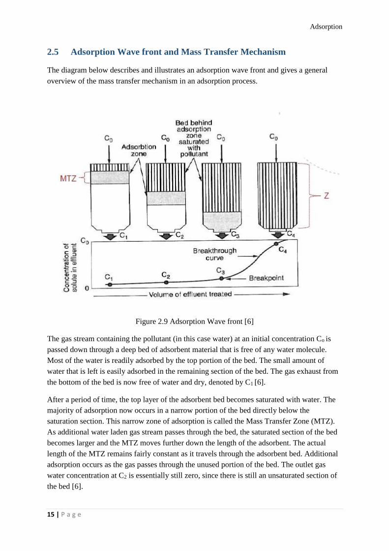
2.5 Adsorption Wave front and Mass Transfer Mechanism
The diagram below describes and illustrates an adsorption wave front and gives a general
overview of the mass transfer mechanism in an adsorption process.
Figure 2.9 Adsorption Wave front [6]
The gas stream containing the pollutant (in this case water) at an initial concentration Co is
passed down through a deep bed of adsorbent material that is free of any water molecule.
Most of the water is readily adsorbed by the top portion of the bed. The small amount of
water that is left is easily adsorbed in the remaining section of the bed. The gas exhaust from
the bottom of the bed is now free of water and dry, denoted by C1 [6].
After a period of time, the top layer of the adsorbent bed becomes saturated with water. The
majority of adsorption now occurs in a narrow portion of the bed directly below the
saturation section. This narrow zone of adsorption is called the Mass Transfer Zone (MTZ).
As additional water laden gas stream passes through the bed, the saturated section of the bed
becomes larger and the MTZ moves further down the length of the adsorbent. The actual
length of the MTZ remains fairly constant as it travels through the adsorbent bed. Additional
adsorption occurs as the gas passes through the unused portion of the bed. The outlet gas
water concentration at C2 is essentially still zero, since there is still an unsaturated section of
the bed [6].

Adsorption
16 | P a g e
Finally, when the lower portion of the MTZ reaches the bottom of the bed, the water
concentration in the outlet gas suddenly begins to rise. This is referred to as the breakthrough
point, where untreated gas is being exhausted from the adsorber (outlet gas with water). If the
inlet gas is not switched to a fresh bed, the concentration of water in the outlet gas will rise
quickly until it approaches the final concentration, given as point C4 [6].
To achieve continuous operation, adsorber must be either replaced or recycled from
adsorption to desorption before breakthrough occurs [6].
2.6 Adsorption Processes
During adsorption process, the gas to be dried or purified is passed down an adsorber column
filled with adsorbent. This adsorbent adsorbs the unwanted component in the gas (water)
continuously until its capacity is exhausted. When this point is reached, the gas has to be
switched to another adsorber for continuous adsorption, or the adsorbent has to be changed or
regenerated. In most commercial applications, including natural gas dehydration, the
adsorbent is regenerated so that it can be used again. For such systems, there is normally
more than one adsorber column, so that while one is in regeneration mode, the other(s) is/are
in adsorption mode to ensure continuous operation.
There are two major ways by which regeneration is done and this is done by changing
parameters like temperature and pressure of the gas. These methods are discussed below;
2.6.1 Temperature Swing Adsorption (TSA)
Regeneration of adsorbent in a TSA process is achieved by an increase in temperature. The
effect of temperature on adsorption equilibrium of a single adsorbate can be seen on the
diagram below [15].
For any given partial pressure of the adsorbate in the gas phase, an increase in the
temperature leads to a decrease in the amount adsorbed. Fr a constant partial pressure P,
temperature increase from T1 to T2 will decrease the equilibrium loading from q1 to q2 [15]. A
relatively modest temperature increase can cause a large decrease in loading. It is therefore
generally possible to desorb any components given a high temperature. It is also important to
ensure that the regeneration temperature does not cause degradation of the adsorbent.

Adsorption
17 | P a g e
Figure 2.10 Temperature Swing Adsorption [15]
In commercial applications, a temperature change alone is not used because there is no
mechanism to remove the desorbed adsorbate from adsorber column. A hot purge gas or
steam is passed through the bed to push out the desorbed components [15].
2.6.2 Pressure Swing Adsorption
Regeneration of adsorbent in PSA process is done by reducing the partial pressure of the
adsorbate. This can be seen below;
Figure 2.11 Pressure Swing Adsorption [16]
Reducing the partial pressure from P1 to P2 causes a reduction in equilibrium loading from q1
to q2.
Changes in pressure can be effected much more quickly than changes in temperature. Thus
the cycle time for PSA processes are typically in the order of minutes and seconds [16]. It is
desirable to operate PSA processes close to ambient temperatures to take advantage of the

Adsorption
18 | P a g e
fact that for a given partial pressure, the amount adsorbed or loading is increased as the
temperature is decreased.
The TSA Process is more suitable and mostly used in LNG and NGL extraction Plants than
the PSA Process. This is because the TSA process gives higher temperatures than PSA
process, and this high temperature is needed to desorb the water molecules from the
adsorbents effectively.
2.7 Adsorption Process Design
One important process design factor is the number of towers. There are different process
configurations for adsorption dehydration systems. The most common arrangements are two-
tower and three-tower systems [17]. Most large dry adsorbent units for natural gas drying
contain more than two towers to optimize the economics of operations [8].
2.7.1 Two-tower adsorption dehydration system
Figure 2.12 Two-tower dehydration system [17]
In the two-tower system, while tower A is in adsorption mode, tower B is in regenerating
mode. After tower A completes it adsorption cycle, it will switch to the regeneration mode
and tower B starts its adsorption cycle. At any time, one of the tower is adsorbing while the
other is regenerating [17].

Adsorption
19 | P a g e
The wet gas is passed through the top of tower A. A mass transfer process takes place
through the bed and dry gas leaves the bed at the bottom. At the same time, tower B is
regenerated by the use of hot and dry gas which is passed through the bottom. The pressure is
normally also reduced. The driving force for the mass transfer process is reversed. The water
molecules adsorbed to the surface of the adsorbent are removed and leaves with the
regeneration gas at the top of tower B. The gas is cooled after the bed and the free liquid
condensed out [3].
In gas dehydration by adsorption, adsorption flow is almost always downward because of the
higher allowable velocity in the downward direction. Upward regeneration is preferred even
though it requires more valves and piping. Most bed contamination occurs at the top. By
regenerating upward, the steam produced at the lower part of the bed helps remove the
contamination without spreading it throughout the bed [8].
2.7.2 Three-tower adsorption dehydration system
Figure 2.13 Three-tower adsorption dehydration system [17]
In the three-tower configuration, at any time, two towers (e.g. A and B) are in parallel
adsorption mode while the third tower (e.g. C) is in regeneration mode. In this configuration,
half of the feed gas flow rate is going through tower A and the other half passes through B as
shown above [17].

Adsorption
20 | P a g e
It is normal to use a three-tower system in order to get a smooth sequence with sufficient time
for heating of bed, regeneration and cooling of bed again. The bed system needs to be
controlled in such a way that the adsorption capacity is not overloaded [3].
Feed gas conditions also have an impact on the adsorption dehydration process. The feed gas
pressure, flowrate and temperature are very important factors that have an effect on the mass
of adsorbent required, bed diameter required and bed height required [18].
Figure 2.14 Variation of adsorbent mass with feed gas rate, temperature and pressure [18]
It can be seen from the above chart that as the gas rate increases, the mass of adsorbent
required increases for a given adsorption time. Feed with higher temperature and lower
pressure requires more mass and the opposite is the case for a feed with lower temperature
and higher pressure [18]. Also, research and past experiments have shown that feed gas with
higher temperature and lower pressure needs a larger diameter bed and taller height while a
feed with lower temperature and higher pressure needs a smaller diameter bed and shorter
height [18].
2.8 Effects of Glycols on Natural Gas Dehydration by Adsorption
In natural gas processing and liquefaction to LNG, most times gas dehydration is normally
done first by absorption process using TEG. Gas dehydration by absorption is done mostly on
offshore plants where the water dew point specification is not so low, to prepare the gas for
pipeline transport to onshore gas processing plants. The onshore plants are usually NGL
extraction and LNG plants where the water dew point specification is much lower than that of

Adsorption
21 | P a g e
offshore plants. Here, gas dehydration by adsorption using solid adsorbents is the preferred
dehydration process because drier gases can be achieved with this process.
Sometimes, some quantities of TEG follows the gas from the absorption process down to the
onshore plants where gas dehydration by adsorption is done. These TEG quantities will have
a negative impact on the efficiency of the adsorption process.
One of the ways by which the adsorption process is negatively impacted by TEG
contamination is through the capacity decline of the adsorbents. Cyclical heating and cooling
of adsorbents results in capacity decline due to gradual loss of crystalline structure and/or
pore closure [19]. A more pronounced cause of capacity decline is contamination of
adsorbents due to liquid carryover (e.g. TEG) from upstream separation equipment [19].
Typical regeneration temperatures are between 200 – 300oC, heating the adsorbent to these
temperatures causes thermal degradation of TEG and instead of TEG to be desorbed, it
degrades and destroys the pore structure of the adsorbent. Glycols cannot be removed by
regeneration process, thereby reducing the capacity of the adsorbent to uneconomic levels in
short periods of time [8]. As the capacity declines in short periods of time, the adsorption
time decreases, and this consequently leads to a higher number of adsorption cycles required.
A high number of adsorption cycle leads to a decrease in life factor of the adsorbent, and if
this decrease is rapid, the adsorbent will need to be changed after a while.
2.8.1 Proposal for the reduction of negative TEG effect on adsorption
Significant savings can be made if the negative effects of TEG contamination on the
adsorption process can be reduced. These savings can be achieved in the form of increased
adsorption capacity of the adsorbent (which means a higher number of cycles).

Adsorption
22 | P a g e
Figure 2.15 A generic molecular sieve decline curves [19]
From the chart above, some important observations can be made;
• The life of the adsorbent and adsorption capacity is a function of the number of
cycles, not the elapsed calendar time
• The curves good, average and poor indicate variation in site specific factors
2.8.1.1 Standby Time in Adsorption Dehydration Process
A gas dehydration by adsorption process is usually designed according to some design
conditions and parameters like the capacity of the adsorption and regeneration, feed gas
temperature, pressure and rate, and other parameters.
If the regeneration circuit has excess capacity that is larger than the normal design conditions,
then this brings about standby time [19]. Because of this excess capacity, the online
adsorption time can be reduced, and the adsorbent beds turned around faster by regenerating
the beds in a shorter cycle time. It is always advisable to design an adsorption unit with 10 –
20% excess regeneration capacity. Available standby time may be able to extend the life of a
molecular sieve adsorbent when the unit is operating on fixed cycle times [19]. It should be
noted that a regeneration cycle consists of heating, cooling, depressurization and
repressurization.
2.8.1.2 Case Study
An analysis has been done by John M. Campbell to illustrate the benefits of standby time.
The case study below has been considered, the unit is expected to run for 3 years before
needing a recharge and the plant turnaround is based on this expectation. The following
assumptions [19];
• Three-tower molecular sieve dehydration unit (2 on adsorption and 1 on regeneration)
• Feed gas rate of 11.3 × 10⁶ std m3/d (400 MMscfd)
• External insulation
• Tower height of 2.9m
• Each tower contains 24630 kg of type 4A 4 × 8 mesh beads
• Regeneration circuit capable of handling an extra 15% of flow
• Unit is operated on fixed cycle times
The table below shows the molecular sieve design summary

Adsorption
23 | P a g e
Parameter Adsorption Heating Cooling Depressure Repressure
Time (hrs/tower) 16 4.88 2.62 0.2 0.2
Flow Direction Down Up Up Down Down
Pressure Drop, Kpa < 50 < 7 < 7
Table 2.2 Molecular sieve design summary
The table below shows the design basis for the case study
Parameter Feed Regeneration Heating Regeneration Cooling
Flow Rate, 106 × std m3/d 11.3 0.71 0.71
Pressure, Kpa 6205 2068 2068
Temperature, oC 30 288 30
Molecular Weight 20.3 17.1 17.1
Water Content Saturated < 0.1 ppmv < 0.1 ppmv
Table 2.3 Design basis for case study
The analysis done here is valid for low pressure regeneration (less than 4100 Kpa). A loading
life factor, FL, of 0.6 after 3 years (1095 cycles) of operation at design condition has been
found using concepts outlined in chapter 18 of the book ‘Gas Conditioning and Processing:
The equipment modules’. This point lies slightly above the average life curve as seen in
Figure 2.16.

Adsorption
24 | P a g e
Figure 2.16 Design condition life factor [19]
2.8.1.3 Case Study Results
After 12 months, a Performance Test Run (PTR) was done and the results is shown in table
2.4 and Figure. 2.17.
Parameter Feed
Flow Rate, 106 × std m3/d 10.9
Pressure, Kpa 6205
Temperature, oC 28
Molecular Weight 20.3
Water Content Saturated
Breakthrough time (hr) 20.9
Table 2.4 Results of PTR after 12 months of operation

Adsorption
25 | P a g e
Figure 2.17 PTR life factor [19]
As can be observed from Figure. 2.17, FL has been determined to be 0.68 after 365 cycles (1
year of operation). Following the PTR curve, the molecular sieves will experience water
breakthrough if operated at design conditions in less than three years [19].
Figure. 2.18 below shows the projected FL after three years of operation of the unit at design
conditions.

Adsorption
26 | P a g e
Figure. 2.18 Projected life factor (red triangle) running at design conditions [19]
If the capacity decline follows the same trend as seen from the PTR, water breakthrough will
occur after just 750 cycles or just over 2 years from start-up at if operations is run at design
conditions (FL = 0.6). This can be illustrated in Figure. 2.19.
Figure 2.19 Projected life factor running at design conditions [19]

Adsorption
27 | P a g e
Because of the excess capacity of 15% the regeneration circuit can handle, the complete
regeneration cycle (heating, cooling, depressurization and repressurization) can be reduced to
7 hours from 8 hours. This allows the bed to turn around faster [19].
Complete cycle time is now 21 hours instead of the initially 24 hours, this gives an FL of 0.53.
This is because less water is being adsorbed per cycle. This reduced FL gives 1500 number of
cycles as shows in Figure. 2.20.
Figure 2.20 Projected life factor (red triangle) if standby time is used [19]
Taking advantage of this standby time and operating at reduce cycle time immediately after
the PTR, the molecular sieves should last an additional 2.7 years, giving a total life of 3.7
years. Therefore, standby time will allow the unit to operate until the scheduled turnaround
[19].
The following conclusions can be noted from the above study [19];
• The above method shown estimates the capacity decline of adsorbent based on only
one PTR for molecular sieves dehydration unit using low pressure regeneration. This
can serve as a foundational plan for corrective actions
• site related factors determine the decline curve of a unit. As a result, it will be useful
to conduct more than one PTR.
• Standby time offers the possibility of prolonging the life and adsorption capacity of an
adsorbent.
• Adsorption capacity is a function of the number of cycles, not calendar time.
Based on the case study above by John M. Campbell, it can be seen that a way to reduce one
of the negative effects of TEG contaminant (capacity decline of adsorbent) in the adsorption

Adsorption
28 | P a g e
process is by the use of standby time to further prolong the number of cycles of the system,
thereby increasing adsorption capacity of the adsorbent.
The above case study has been analysed using the Gas Conditioning and Processing (GCAP)
software. This software is discussed in the next chapter.
2.9 Section Summary
This chapter has been an extensive one in which Adsorption Dehydration has been discussed
in details, as that is the focus of the project work.
Fundamentals of adsorption has been looked at, as well as the types of adsorption forces,
various relevant adsorbents and their properties and applications, selection of adsorbents,
adsorption isotherms and the relevant models, adsorption capacity and regeneration
processes.
Important factors in adsorption design has also been discussed as well as two-tower and
three-tower system.
Also, the chapter has been concluded by examining the effect of TEG contamination on an
adsorption process. A case study done by John M. Campbell has been looked at. The results
of the case study show that standby time in adsorption process can be used to mitigate a
negative effect of TEG contamination by extending the number of cycles of an adsorption
process, thereby increasing the adsorption capacity of an adsorbent (molecular sieve).

Adsorption Simulation Tools and Models
29 | P a g e
3 Adsorption Simulation Tools and Models
There are various tools and models that can be used to simulate gas dehydration by
adsorption processes.
3.1 Adsorption Simulation Tools
One of the simulation tools that was looked at is the ProSim DAC. This software has been
developed by ProSim for Dynamic Adsorption Column Simulation. In this software, both the
TSA and PSA can be modelled. This tool can be used to conduct in-depth analysis of solid-
gas adsorption operations including refinery hydrogen purification, isotopic separation,
emission control, solvent recovery and other industrial applications. This software has been
mainly used in nuclear air treatment and hydrogen studies [20].
Some limitations have been encountered in the use of ProSim DAC. Firstly, most of its
applications have been found to be around emissions control and gas cleaning, very limited
application has been seen in natural gas dehydration. Also, in trying to get access to this
software, it offers just a ten-day trial usage, which is quite short considering that one would
like to get acquainted to this software and see the possibility of it being used for the project.
Consequently, this software was not considered.
Another software that was considered is Aspen HYSYS. This is a good software for process
simulation and optimization. On checking to see if this was suitable, it was noticed that
adsorption columns were not included in the unit toolbar to choose from. Hence this was not
considered. Instead, aspentech has developed a separate simulation tool for modelling and
simulation of adsorption process, called Aspen Adsorption. From previous experience with
Aspen HYSYS and from materials and demo performances, it has been seen that this
software is a comprehensive flowsheet simulator for designing an adsorption process.
However, access to this software could not be gotten now so it was not considered.
The most user friendly and readily available software that was considered is called the Gas
Conditioning and Processing (GCAP) Software. This software is discussed below.
3.1.1 Gas Conditioning and Processing Software
The GCAP software was developed by PetroSkills, John M. Campbell. The GCAP has been
designed to give quick checks and relatively easy analysis to very complicated calculations
[21]. This software is based on the equations and correlations used in the ‘Gas Conditioning
and Processing’ textbook by John M. Campbell. Since this textbook has been used during
lectures, and ideas have been gotten from it in the development of the project work, this
software appears to be suitable to consider.

Adsorption Simulation Tools and Models
30 | P a g e
Also, this software has been found to have a good user friendly interface, with some
instructions on how to get started with it. Also, a trial version of this software has been made
available online and this lasts for 90 days, this gives a reasonably good length of time to refer
to this software and use it more critically if the need arises at later stages of the project. The
GCAP is also mostly a graphical simulation software that gives a graphical analysis of
various simulations based on input data and calculated data.
3.1.1.1 Software and topic selections
The GCAP software has different volumes in which the different chapters of the Campbell
textbook are treated. For each chapter, there is a different working or simulation environment
for which simulations can be done based on the topic of the chapter.
Figure 3.1 Selection of topics to run simulations
For the chapter that is of relevance to this project, it is chapter 18, which is adsorption
dehydration. This is discussed below.
3.1.1.2 Adsorption Dehydration chapter
Chapter 18 is about performance evaluation for an existing molecular sieve dehydration plant
and this is divided into two sections. Section one is about simulations done to determine
molecular sieve equilibrium loading and the second section is about evaluation analysis and
performance prediction of an adsorption column.
For the case study done in chapter 2.8.1.2, the second section of chapter 18 of the software
has been used. In this section, the user interface allows one to enter some input parameter

Adsorption Simulation Tools and Models
31 | P a g e
such as design gas temperature, pressure, feed rate. This can be seen below. After this has
been done, the simulation is the run and the results are displayed graphically.
Figure 3.2 specifying input parameters
Figure 3.3 Graphical representation of analysis

Adsorption Simulation Tools and Models
32 | P a g e
Figure 3.3 is a single graphical representation of the four graphs shown in chapter 2.8.1.2.
This the various scenarios that occur in evaluating the capacity decline and loading life factor
of a molecular sieve.
As a summary of tools used to simulate adsorption processes, GCAP was found to be the
handiest tool to come by, after efforts in exploring the possibilities of using other tools.
3.2 Adsorption Models
There are different models that have been used in the past when describing adsorption
processes. These models can be based on the adsorption kinetics or adsorption diffusion.
Predicting the rate at which adsorption takes place for a given system is one of the most
important factors in adsorption system design, with adsorbate residence time and reactor
dimensions controlled by the system’s kinetics [22]. To investigate the mechanisms of
adsorption, various kinetic models have been suggested. In recent years, adsorption
mechanisms involving kinetics – based models have been reported. Numerous kinetic models
have described the reaction order of adsorption systems based on solution concentration,
these include first and second order reversible models, pseudo – first – order and pseudo –
second – order models based on solution concentration [22]. Other kinetic models have also
described the reaction order based on adsorbent capacity, these include Lagergren’s first –
order equation, Zeldowitsch’s model, and Ho’s second – order expression [22].
This section considers a selected few models of adsorption process.
3.2.1 Second – Order Rate Equation
A linear form of the second – order rate equation is
1
𝐶𝑡= 𝑘2𝑡 +
1
𝐶0 3.1
Where Ct is the equilibrium concentration (mg/dm3), C0 the initial concentration (mg/dm3), t
is the time (min) and K2 is the rate constant (dm3/mg min).
Early applied second – order rate equations in solid/liquid systems described reactions
between soil and soil minerals [22]. Other applications included the adsorption of fluoride
onto acid – treated spent bleaching earth and the adsorption of water using the dealumination
of HZSM-5 zeolite by thermal treatment [22].
3.2.2 Lagergren’s Equation
Lagergren’s equation is a kinetic model that describes the reaction order based on adsorbent
capacity. In 1898, Largergren described the liquid – solid phase adsorption systems, which
consisted of the adsorption of oxalic acid and malonic acid onto charcoal. Lagergren’s first –

Adsorption Simulation Tools and Models
33 | P a g e
order rate equation is the earliest known one describing the adsorption rate based on the
adsorption capacity of the adsorbent [22]. It is summarised as follows;
𝑑𝑥
𝑑𝑡= 𝑘 (𝑋 − 𝑥) 3.2
Where X and x (mg/g) are the adsorption capacities at equilibrium and at time t (min),
respectively, and k is the rate constant of the first – order adsorption (l/min).
Equation 3.2 was integrated with the boundary conditions of t = 0 and t = t and x = 0 and x =
x to yield;
𝐼𝑛𝑋
𝑋−𝑥= 𝑘𝑡 3.3
and
𝑥 = 𝑋(1 − 𝑒−𝑘𝑡) 3.4
Equation 3.3 can be linearized to give;
log(𝑋 − 𝑥) = log(𝑋) − 𝑘
2.303𝑡 3.5
To distinguish kinetics equations based on concentrations of solution from adsorption
capacities of solids, Lagergren’s first – order rate equation has been called pseudo – first –
order [22]. An early known application of Lagergren’s kinetics equation to adsorption was
undertaken by Trivedi et al. for the adsorption of cellulose triacetate from chloroform onto
calcium silicate. The kinetics equation has been widely applied to the adsorption of pollutants
from aqueous solutions [22].
3.2.3 Elovich’s Equation
Elovich’s equation is another rate equation based on the adsorption capacity [22]. In 1934,
the kinetic law of chemisorption was established through the work of Zeldowitsch. The rate
of adsorption of carbon monoxide on manganese dioxide decreasing exponentially with an
increase in the amount of gas adsorbed was described by Zeldowitsch. It has commonly been
called the Elovich equation in the following years [22].
𝑑𝑞
𝑑𝑡= 𝑎𝑒−∝𝑞 3.6
Where q is the quantity if gas adsorbed during the time t, ∝ the initial adsorption rate, and a is
the desorption constant during any one experiment. Equation 3.6 can be integrated and
written as;
𝑞 = 2.3
∝ log (𝑡 + 𝑡0) −
2.3
∝ 𝑙𝑜𝑔𝑡0 3.7

Adsorption Simulation Tools and Models
34 | P a g e
and 𝑡0 = 1
∝𝑎 3.8
The Elovich equation is commonly used to determine the kinetics of chemisorption of gases
onto heterogeneous solids, and is quite restricted, as it only describes a limiting property
ultimately reached by the kinetic curve [22].
3.2.4 Ritchie’s Equation
in 1977, Ritchie developed a model for the adsorption of gaseous systems. Assumptions
made for this model are that; θ is the fraction of surface sites which are occupied by an
adsorbed gas, n the number of surface sites occupied by each molecule of the adsorbed gas
and ∝ is the rate constant [22]. Assuming that the rate of adsorption depends solely on the
fraction of sites which are unoccupied at time t, then;
𝑑θ
𝑑𝑡=∝ (1 − θ)𝑛 3.9
Integrating equation 3.9 gives;
1
(1−θ)𝑛−1 = (𝑛 − 1) ∝ 𝑡 + 1 for n ≠ 1 3.10
Several adsorption results have been analysed using the Ritchie equation. The Ritchie
equation has been used in contrast or comparison with the Elovich equation and in cases
where the systems did not fit the Elovich equation, Ritchie equation has been found to give
better results [22].
3.2.5 Thomas Model
The Thomas model has also been frequently applied in the analysis and estimation of the
adsorption capacity of adsorbents and prediction of breakthrough curves, assuming the
second – order reversible reaction kinetics and the Langmuir isotherm [23]. For theoretical
studies, it is suitable to estimate the adsorption process where the external and internal
diffusion resistances are extremely small. The Thomas model is given by the following
equation;
𝐼𝑛 (𝐶𝐹
𝐶− 1) =
𝐾𝑇ℎ𝑞𝐹𝑚
𝑄− 𝑘𝑇ℎ𝐶𝐹𝑡 3.11
Where KTh is the Thomas rate constant, m is the mass of adsorbent in the column. With
several couples of m and Q, KTh and qF values can be derived through a plot of In[(CF/C)-1]
vs t, further prediction and design can then be carried out.
Equation 3.11 can be expressed as;
𝐼𝑛 (𝐶𝐹
𝐶− 1) = 𝑘′(𝑡 − 𝑡1) 3.12

Adsorption Simulation Tools and Models
35 | P a g e
Where k’=KThCF and t1=qFm/ (QCF). It is important to note that the qF derived
experimentally most time differs from the value determined from equilibrium calculations,
and the bed adsorption capacity is often determined from the dynamic adsorption [23].
3.2.6 The Linear Driving Force Model
The Linear Driving Force (LDF) model is a model that is also based on the kinetics of gas
adsorption, and has been frequently and successfully used in the analysis of adsorption
column dynamics and adsorptive process designs [24]. The LDF model has been found to be
simple, analytic and physically consistent.
The LDF model was originally proposed by Gleuckauf and Coates in 1947 for adsorption
chromatography [24]. Mathematical simulation of cyclic gas separation processes such as
TSA or PSA requires models for describing adsorption kinetics, and the LDF model has been
frequently used for this purpose [24].
The rate of adsorption of a single adsorbate (pure gas or mixture with an inert gas) into an
adsorbent particle according to the LDF model is given by;
𝑑C(t)
𝑑𝑡= 𝑘𝐿[𝐶∗(𝑡) − 𝐶(𝑡)] 3.13
Where C(t) is the average adsorbate concentration (moles per unit volume) in the adsorbent
particle at time t, and C*(t) is the adsorbate concentration in the particle that would be in
equilibrium with the instantaneous superincumbent gas phase partial pressure of the
adsorbate [P(t)] and the adsorbate temperature [T(t)] at time t. The LDF model assumes that
the adsorbent particle temperature is uniform (does not vary with radius) at all times [24].
The variable kL is called the effective LDF mass transfer coefficient at adsorbate loading of C
and temperature T. The average adsorbate loading (moles per unit weight) at time t is given
by n(t) = C(t)/ 𝜌p where 𝜌p is the adsorbate particle density.
The table below reproduces the analytical expressions for f(t) obtained under isothermal,
constant volume and constant pressure experiments for the LDF model.
Models Constant pressure experiment Constant volume experiment
LDF 𝑓(𝑡) = 1 − 𝑒−𝑘𝐿𝑡 𝑓(𝑡) = 1 − 𝑒−(1+∝)
𝑘𝐿∝
Table 3.1 Analytical batch uptake curves [24]
3.2.6.1 Effect of Adsorbent Heterogeneity
In principle, most amorphous and bounded crystalline adsorbents are heterogeneous,
consisting of a network of interconnected pores of different sizes, shapes and surface
chemistry [24]. Quantitative estimation of such heterogeneity is not practically possible by
modern technology. Consequently, the uptake profiles measured by experiments on these
adsorbents already reflect the average rate of adsorption by the composite pore structure of
the adsorbent [24].

Adsorption Simulation Tools and Models
36 | P a g e
While making the assumption that the heterogeneous adsorbent consists of a collection of
parallel pores, each having a different kL value, the averaging effect was evaluated [24]. A
normalized gamma distribution function was assumed to represent the adsorbent
heterogeneity. Thus, the average fractional uptake [F(t)] at time t by the heterogeneous
adsorbent for a constant pressure experiment is given by;
𝐹(𝑡) = ∫ 𝑓(𝑡). 𝜆(𝑥)𝑑𝑥∞
0 3.14
Where f(t) is the local fractional uptake at time t by a pore characterized by the property x
(kL). The function 𝜆(𝑥) is the probability density function for the distribution of the property
x in the adsorbents.
𝜆(𝑥) =𝑎(𝑝+1)
Γ(𝑝+1). 𝑥𝑝 . 𝑒−𝑞𝑥 3.15
∫ 𝜆(𝑥)𝑑𝑥∞
0= 1 3.16
Where Γ is the gamma function. The variables and p are two adjustable parameters of the
gamma distribution. The mean 𝜇 and variance 𝜎 of the gamma distribution are given by;
𝜇 =(𝑝+1)
𝑎; 𝜎2 =
(𝑝+1)
𝑎2 3.17
Integrating equation 3.14 using the local uptake characteristics [f(t)] for the LDF model in
Table 3.1 and combining it with equation 3.15 – 3.17 gives;
𝐹(𝑡) = 1 − [1
1𝑥
1+𝜇𝑥𝑡1𝑥
] 3.18
Where x is defined by (𝜎/𝜇)2. The variable x is a measure of the degree of heterogeneity of
the adsorbent. The adsorbent is homogenous when x = 0. Equation 3.18 reduce to the uptake
expression for homogenous system given in Table 3.1.
3.2.7 Pseudo – second – order Kinetic Equation
The pseudo – second – order kinetic equation has been most widely used in the study of
adsorption kinetics to describe time evolution of adsorption under nonequilibrium conditions
[25]. The equation is given as;
𝑑𝑄𝑡
𝑑𝑡= 𝑘′
2(𝑄𝑒 − 𝑄𝑡)2 3.19
Where Qt is the amount of adsorbate adsorbed at time t, Qe is its value at equilibrium and 𝑘′2
is constant. In many cases of adsorption studies, it has been claimed that equation 3.19 can
provide satisfactory description of adsorption data obtained under various experimental
conditions [25]. Integrating equation 3.19 gives;

Adsorption Simulation Tools and Models
37 | P a g e
𝑄𝑡 =𝑄𝑒
2𝑘2′ 𝑡
𝑘2′ 𝑄𝑒𝑡+1
3.20
Equation 3.20 can be linearized to various expressions to determine the constants involved. It
can be translated into the following linear relationship between 1/Qt and 1/t;
1
𝑄𝑡=
1
𝑄𝑒2𝑘2
1
𝑡+
1
𝑄𝑒 3.21
Equation 3.19 has been regarded as an empirical formula, and its integrated form appears
complex without clear mathematical structure [25].
3.3 Heat Transfer Models for Packed Beds
In this section, some models for heat transfer in packed beds have been reviewed. During
adsorption and desorption processes, there is usually heat and mass transfer between the
adsorption or regeneration gas, the wall of the adsorption column and the adsorbent bed.
Therefore, this is an important part of modelling an adsorption or desorption process. It is
essential to be able to see the interaction and temperature profiles of the gas as it travels
through the adsorption column, as well as the column walls and the adsorbent temperature
profiles. Heat transfer plays a crucial role in determining and evaluating the performance of
packed beds in chemical and process industries.
There are many heat transfer models that have been established in previous works, some of
which have been discussed below;
3.3.1 Heterogeneous Model for Heat Transfer in Packed Beds
This model has been suggested by R.J. Wijngaarden and K.R. Westerterp. An adsorption or
desorption process takes place in a packed bed, packed with adsorbents, mostly molecular
sieves because of its high water capacity. Heat transfer interaction occurs between the gas,
adsorbent and walls of the packed column. The heterogeneity of the bed is an important
factor because of the heat flow between the adsorbent pellets and the gas [26]. There are
global heat parameters for the packed bed, such as the effective radial heat conductivity 𝜆𝑒𝑓𝑓
and wall heat transfer coefficient ∝𝑤 and they are derived from homogeneous models,
therefore the values of 𝜆𝑒𝑓𝑓 and ∝𝑤 can be attributed to the gas phase, solid phase or both
phases [26]. It is assumed that the heat transfer in the solid and gas phase occurs in series by
three mechanisms;
• Heat transfer from the solid to the gas, described by the pellet heat transfer
coefficient, ∝𝑝
• Heat transfer through the gas to the outer wall, described by 𝜆𝑒𝑓𝑓
• Heat transfer at the wall through the gas, given by ∝𝑤

Adsorption Simulation Tools and Models
38 | P a g e
These assumptions were used to describe the changing radial and axial temperature profiles
in the packed bed.
The experimental procedure for this model consists of a packed bed elevated to constant
temperature, with the wall temperature being the same. The gas flow was cold air.
Thermocouples were shoved in the packed bed at varying radial distances to measure
temperature as a function of radial position, axial position and time. The gas temperatures
were obtained, not the pellet temperatures [26]. The pellet material used was an industrial
ring – shaped catalyst.
Some assumptions were made in the development of this model [26];
• Accumulation of heat in the gas phase can neglected
• Axial dispersion of heat in both the solid and the gas phase is neglected, as well as
heat conduction within the particles
• Radial porosity, velocity and heat conduction profiles were not incorporated in the
model.
With the above assumptions, a heat balance for an infinitesimally small ring in the packed
bed yields;
𝜕𝜃𝑔
𝜕𝜔−
1
𝑃𝑒𝛳 1
𝑝
𝜕
𝜕𝑝(𝑝
𝜕𝜃𝑔
𝜕𝑝) + 𝑆𝑡𝛳(𝜃𝑔 − 𝜃𝑘) = 0 3.22
𝑆𝑡𝛳(𝜃𝑔 − 𝜃𝑘) −𝜕𝜃𝑘
𝜕𝜏= 0 3.23
Subject to initial conditions
𝛚 = 0 ==> 𝜃𝑔 = 𝜃𝑖𝑛 3.24
𝜏 = 0 ==> 𝜃𝑘 = 𝜃𝑏 3.25
and the boundary conditions
𝑝 = 1 → 𝜕𝜃𝑔
𝜕𝑝= 𝐵𝑖𝑐
𝛳𝜃𝑔 3.26
𝑝 = 1 → 𝜕𝜃𝑔
𝜕𝑝= 𝐵𝑖ℎ
𝛳(1 − 𝜃𝑔) 3.27
Equations 3.22 – 3.27 are solved to yield a formula with which the dimensionless
temperatures 𝜃𝑔 and 𝜃𝑘 can be calculated as a function of 𝛚, p and 𝜏 for any chosen values of
𝑃𝑒𝛳, 𝑆𝑡𝛳, 𝐵𝑖𝑐𝛳 and 𝐵𝑖ℎ
𝛳 [26].
𝜃𝑔, 𝜃𝑖𝑛, 𝜃𝑘, 𝜃𝑏= dimensionless gas temperature, dimensionless inlet gas temperature,
dimensionless pellet temperature and dimensionless initial bed temperature respectively.
𝛚 is dimensionless axial coordinate
Adsorption Simulation Tools and Models
39 | P a g e
𝑃𝑒𝛳 is modified Peclet number based on tube dimensions
P is dimensionless radial coordinate
𝑆𝑡𝛳 is modified Stanton number
𝐵𝑖𝑐𝛳, 𝐵𝑖ℎ
𝛳 is modified Biot number at the cold wall and hot wall respectively
𝜏 is dimensionless time
All heat transfer properties in a packed bed are considered as lumped parameters, and model
deviations are lumped in the values of these properties [26]. This is a series model and there
are reasons why this model is considered to be close to reality, since no model matches
reality completely; the static contribution of the effective heat conductivity of the bed
depends on the heat conductivity of the solid phase, this agrees with the series model [26].
This model has been recommended for use in packed bed heterogeneous models.
3.3.2 Equivalence of One and Two – Phase Models for Heat Transfer Processes in
Packed Beds: One Dimensional Theory
For a fixed bed through which gas is flowing with or without chemical reaction, there are two
general types of models used to describe the mathematical analysis of heat and mass transfer
processes [27], these are;
• The group of one – phase models in which the bed is approximated by a quasi –
homogeneous medium.
• The group of two – phase models in which both phases exchange heat and/or mass;
these transport processes are treated independently.
The two – phase model appears to be the more realistic of the two [27]. The energy balances
of the two groups of models contain various transport coefficients and this model has
attempted to derive an expression that relates these coefficients [27]. It has also been shown
that the total energy dispersion, as represented by the axial effective thermal conductivity, is
due to the sum of the individual dispersive mechanisms including the stagnant bed thermal
conductivity, gas – solid heat transfer and intraparticle conduction [27].
Two – Phase Model
For calculation of heat transfer processes in packed beds and heat regenerators, Anzelius and
Schumann applied the following energy balances;
Gas 𝜖𝜌𝑓𝐶𝑓𝜕𝑇
𝜕𝑡= − ṁ𝑓𝐶𝑓
𝜕𝑇
𝜕𝑥+ ℎ𝑎(𝜃 − 𝑇) 3.28
Solid (1 − 𝜖)𝜌𝑠𝐶𝑠𝜕𝜃
𝜕𝑡= ℎ𝑎(𝑇 − 𝜃) 3.29
Where T and 𝜃 are the gas and solid temperatures respectively; h is the heat transfer
coefficient based on the average particle temperature and a is the particle surface area per unit

Adsorption Simulation Tools and Models
40 | P a g e
volume of bed. These equations are applicable for large Reynolds numbers [27]. For small
Reynolds numbers, Littman and Silva have shown that equation 3.29 should be expanded to
include a term accounting for axial heat conduction in the bed. Analysis of their frequency
response measurements gave the following model [27];
Gas 𝜖𝜌𝑓𝐶𝑓𝜕𝑇
𝜕𝑡= − ṁ𝑓𝐶𝑓
𝜕𝑇
𝜕𝑥+ ℎ𝑎(𝜃 − 𝑇) 3.30
Solid (1 − 𝜖)𝜌𝑠𝐶𝑠𝜕𝜃
𝜕𝑡= ℎ𝑎(𝑇 − 𝜃) + (1 − 𝜖)𝜆 ∗𝑠
𝜕2𝜃
𝜕𝑥2 3.31
Introducing a corresponding axial conduction term in the gas phase energy balance was found
to be unnecessary [27]. With further assumption that the thermal capacity of the gas phase is
much smaller than that of the solid phase, and therefore can be neglected, the energy balances
become;
Gas ṁ𝑓𝐶𝑓𝜕𝑇
𝜕𝑥+ ℎ𝑎(𝑇 − 𝜃) = 0 3.32
Solid (1 − 𝜖)𝜌𝑠𝐶𝑠𝜕𝜃
𝜕𝑡= ℎ𝑎(𝑇 − 𝜃) + 𝜆0
𝜕2𝜃
𝜕𝑥2 3.33
Equations 3.32 and 3.33 require initial and boundary conditions. For initial conditions, the
solid phase will have some initial temperature profile 𝜃 = 𝜃(𝑥, 0) [27].
One – Phase Model
With the assumption that the thermal capacity of the gas phase can be neglected, the energy
balance for the one – phase model is given as;
(1 − 𝜖)𝜌𝑠𝐶𝑠𝜕𝜗
𝜕𝑡= 𝜆𝑎𝑥
𝜕2𝜗
𝜕𝑥2− ṁ𝑓𝐶𝑓
𝜕𝜗
𝜕𝑥 3.34
The 𝜆𝑎𝑥 parameter is the axial effective thermal conductivity of the bed, and Yagi et al.
determined experimentally that;
𝜆𝑎𝑥 = 𝜆0 + 𝛿𝑅𝑒𝑃𝑟𝜆𝑓 3.35
Where
0.7 < 𝛿 < 0.8 3.36
Derivation of the one – phase model from the two – phase model
Subtraction equation 3.32 from 3.33 gives;
(1 − 𝜖)𝜌𝑠𝐶𝑠𝜕𝜃
𝜕𝑡= 𝜆0
𝜕2𝜃
𝜕𝑥2 − ṁ𝑓𝐶𝑓𝜕(𝑇−𝜃)
𝜕𝑥− ṁ𝑓𝐶𝑓
𝜕𝜃
𝜕𝑥 3.37
From equation 3.32 one obtains;

Adsorption Simulation Tools and Models
41 | P a g e
−𝜕(𝑇−𝜃)
𝜕𝑥=
ṁ𝑓𝐶𝑓
ℎ𝑎
𝜕2𝑇
𝜕𝑥2 3.38
Substituting equation 3.38 into 3.37 gives;
(1 − 𝜖)𝜌𝑠𝐶𝑠𝜕𝜃
𝜕𝑡= 𝜆0
𝜕2𝜃
𝜕𝑥2+
ṁ𝑓2𝐶𝑓
2
ℎ𝑎
𝜕2
𝑇
𝜕𝑥2 − ṁ𝑓𝐶𝑓𝜕𝜃
𝜕𝑥 3.39
If an assumption is made that;
𝜕2𝑇
𝜕𝑥2 =𝜕2𝜃
𝜕𝑥2 3.40
The following is obtained;
(1 − 𝜖)𝜌𝑠𝐶𝑠𝜕𝜃
𝜕𝑡= (𝜆0 +
ṁ𝑓2𝐶𝑓
2
ℎ𝑎)
𝜕2𝜃
𝜕𝑥2− ṁ𝑓𝐶𝑓
𝜕𝜃
𝜕𝑥 3.41
Equation 3.41 is mathematically identical to the one – phase energy balance.
Comparison of equation 3.34 and 3.41 shows that;
𝜆𝑎𝑥 = 𝜆0 +ṁ𝑓
2𝐶𝑓2
ℎ𝑎 3.42
From the model demonstrations, above, the equivalence of the one and two – phase models
have been demonstrated. It is not necessary for the gas and solid temperatures to be equal
[27]. This equivalence has been demonstrated for an initially cold packed bed of glass beads
heated by a hot air stream.
3.3.3 Two – Dimensional Axial Dispersion Plug Flow Model (2DADPF)
This model is based on a study of both the transient and steady state heat transfer behaviour
of a gas flowing through a packed bed under constant wall temperature conditions [28]. The
effective thermal conductivities and convective heat transfer coefficient are derived based on
the steady state measurements and the two – dimensional axial dispersion plug flow
(2DADPF) model [28]. The 2DADPF model predicts the axial temperature distribution to an
extent, but the prediction is poor for the radial temperature distribution. The suspected reason
for this is the length – dependent behaviour of the effective heat transfer parameters and non
– uniform flow behaviour of the gas.
These effective parameters are obtained by various ways; one is by solving the inverse
problems using various macroscopic models such as the one – dimensional model which
contains an overall heat transfer coefficient (U). A more advanced approach is the use of the
two – dimensional models with either a plug flow (2DPF) or an axially dispersed plug flow
assumption (2DADPF) [28]. The 2DADPF model makes use of the axial dispersion term
(keax). These models are grouped into one – phase homogeneous and the two – phase

Adsorption Simulation Tools and Models
42 | P a g e
heterogeneous models depending on the temperature difference between the flowing fluid
and the packed particle. If the temperature difference between the bulk fluid phase and the
solid phase is small, the one – phase homogeneous model is used, if the temperature
difference is large, the two – phase heterogeneous model is used [28].
The criterion for choosing a model is usually based on the Biot number defined as the ratio of
the thermal resistance within the packed particles to that between the fluid and packed
particles. If the Biot number is smaller than ~ 0.05 then the one – phase model would be more
appropriate [28].
For the derivation of the effective heat transfer parameters, the temperature difference
between the particle surface and surrounding gas was chosen to be small, the two –
dimensional homogeneous model was used. An energy balance under steady state condition
gives;
𝐺𝐶𝐹𝜕𝑇
𝜕𝑥= 𝑘𝑒𝑟
1
𝑟
𝜕
𝜕𝑟(𝑟
𝜕𝑇
𝜕𝑟) + 𝑘𝑒𝑎𝑥
𝜕2𝑇
𝜕𝑥2 3.43
Where G is the gas flowrate, CF is the gas phase specific heat, x and r are the axial and radial
co – ordinates respectively, T is the temperature, ker and keax denote the effective radial and
axial thermal conductivities respectively. Equation 3.43 is the 2DADPF model, which at the
intermediate and high flowrates, reduces to;
𝐺𝐶𝐹𝜕𝑇
𝜕𝑥= 𝑘𝑒𝑟
1
𝑟
𝜕
𝜕𝑟(𝑟
𝜕𝑇
𝜕𝑟) 3.44
Equation 3.44 is the 2DPF model. At the column wall, the boundary condition for 2DADPF
model is given as;
−𝑘𝑒𝑟𝜕𝑇
𝜕𝑥= ℎ𝑤(𝑇𝑤 − 𝑇) 3.45
ℎ𝑤 is the effective fluid – wall heat transfer coefficient and Tw the wall temperature. At the
inlet of the column, a uniform temperature distribution is often assumed;
𝑇 = 𝑇0 3.46
Solutions to equations 3.43, 3.45 and 3.46 can be gotten if ker, keax and ℎ𝑤 are all known, or if
the temperature field is known, it is possible to solve the inverse problem to obtain these
effective parameters [28]. The 2DADPF model assumes a uniform porosity distribution in
packed beds and neglects the radial flow distribution. This assumption could work for beds
with large bed to particle diameter ratios (dt/dp) but significant deviations are expected for
small (dt/dp) ratios due to considerable wall effects [28].
It has also been proven that the effective parameters in the 2DPF and 2DADPF models are
not constant. Previous works by Li and Finlayson, 1977 and Paterson and Carberry, 1983
suggests that the effective thermal conductivities and the wall heat transfer coefficient

Adsorption Simulation Tools and Models
43 | P a g e
decrease with increasing heating length and approach constant values at x = ~400mm after
which the flow is fully developed [28].
3.3.4 An Improved Equation for the overall Heat Transfer Coefficient in Packed Beds
A one – point collocation analysis has been performed on the two – dimensional
pseudohomogeneous model of a foxed bed heat exchanger. This analysis is developed on the
concept of a single radial collocation point whose position depends in the wall Biot number
[29]. There has been a lot of studies on modelling of heat transfer in fixed beds. Recent
studies, in the light of higher computational capabilities, have been towards more complex,
two – dimensional heterogeneous models with spatially variable velocities and transport
properties [29]. By detailed modelling of the fundamental phenomena occurring within the
reactor, the behaviour of the fixed bed reactor has been understood better, and this has been
the goal of such simulations. An equally important goal for such studies and simulations is to
represent a few selected features of reactor behaviour using a simpler model suitable for fast,
repetitive calculations in studies of design, control, parameter sensitivity, etc. [29].
For these reasons, there is consistent growth in interest and studies on the one – dimensional
pseudohomogeneous model, using an overall tube – side transfer coefficient U to account for
radial heat transfer. The coefficient U depends on some process variables, and the difficulty
of finding general empirical correlations for it has led to the widely accepted approach of
relating U to the parameters of the two – dimensional model [29]. The usual relation for U
has been;
1
𝑈=
1
ℎ𝑤+
𝑅𝑡/𝛽
𝑘𝑟 3.47
Where 𝑘𝑟 and ℎ𝑤 are independently correlated or may be further related to more
fundamental parameters.
Classical development
The two – dimensional pseudohomogeneous model for a fixed bed heat exchanger with cold
incoming fluid at x = 0, being heated from a constant temperature wall (x>0), is;
1
𝑃𝑒𝐴
𝜕2𝜃
𝜕𝑥2+
1
𝑃𝑒𝑅(
𝜕2𝜃
𝜕𝑦2+
1
𝑦
𝜕𝜃
𝜕𝑦) =
𝜕𝜃
𝜕𝑥 3.48
With
𝜃 → 0 𝑎𝑠 𝑥 → −∞ 3.49
𝜃 → 1 𝑎𝑠 𝑥 → ∞ 3.50
𝜕𝜃
𝜕𝑦= 0 𝑎𝑡 𝑦 = 0 3.51

Adsorption Simulation Tools and Models
44 | P a g e
𝜕𝜃
𝜕𝑦= 𝐵𝑖(1 − 𝜃) 𝑎𝑡 𝑦 = 1 3.52
Where the axial conduction term and the axial boundary conditions have been included for
completeness and have no effects on the results.
The analytical solution of equation 3.48 to 3.52 has been given by Gunn and Khalid, for x > 0
to be [29];
𝜃(𝑥, 𝑦) = 1 − ∑𝐵𝑖(1+𝛽𝑖)𝐽0𝜆𝑖𝑦
(𝐵𝑖2+𝜆12)𝛽𝑖𝐽0𝜆𝑖
∞𝑖=1 ×𝑒𝑥𝑝 [−
𝑃𝑒𝐴(𝛽𝑖−1)𝑥
2] 3.53
Where
𝛽𝑖 = √1 +4𝜆𝑖
2
𝑃𝑒𝐴𝑃𝑒𝑅 3.54
and the eigen values satisfy the characteristic equation
𝐵𝑖𝐽0(𝜆𝑖) = 𝜆𝑖𝐽1(𝜆𝑖) 3.55
From the expressions above, θ can be evaluated at y=0 or at y=1, and the radial average�̅� can
be obtained. The overall heat transfer coefficient U (with respect to the bed average
temperature) and U’ (with respect to bed centre temperature) can be defined by [29];
𝑈(𝑥)(�̅�(𝑥) − 1) = ℎ𝑤(𝜃(𝑥, 1) − 1) 3.56
and
𝑈′(𝑥)(𝜃(𝑥, 0) − 1) = ℎ𝑤(𝜃(𝑥, 1) − 1) 3.57
Generally, both overall coefficients must be functions of x in order to match the radial energy
flux at every x [29].
The development above is the classical development and can result only in expressions of the
form of equation 3.47 for the limits of Bi 0 and Bi ∞. A more flexible approach is
needed that can give an equation for the entire range of Bi [29].
One – point collocation development
The symmetry of the problem is reflected by the change of variable 𝑢 = 𝑦2 and this gives;
1
𝑃𝑒𝐴
𝜕2𝜃
𝜕𝑥2+
4
𝑃𝑒𝑅(𝑢
𝜕2𝜃
𝜕𝑢2+
𝜕𝜃
𝜕𝑢) =
𝜕𝜃
𝜕𝑥 3.58
with
𝜃 𝑓𝑖𝑛𝑖𝑡𝑒 𝑎𝑡 𝑢 = 0 3.59

Adsorption Simulation Tools and Models
45 | P a g e
𝜃 → 0 𝑎𝑠 𝑥 → −∞ 3.60
𝜃 → 10 𝑎𝑠 𝑥 → ∞ 3.61
𝜕𝜃
𝜕𝑢=
𝐵𝑖
2(1 − 𝜃) 𝑎𝑡 𝑢 = 1 3.62
Applying one – point collocation at 𝑢 = 𝑢1, we set;
𝜃(𝑢) =1−𝑢
1−𝑢1𝜃1 +
𝑢−𝑢1
1−𝑢1𝜃2 3.63
Substituting equation 3.63 into 3.62, solving for θ2 in terms of θ1. Differential equation 3.58
is then collocated to obtain;
𝜕2𝜃1
𝜕𝑥2− 𝑃𝑒𝐴
𝜕𝜃1
𝜕𝑥− 𝐻(𝜃1 − 1) = 0 3.64
Where
𝐻 =4𝑃𝑒𝐴
𝑃𝑒𝑅(1−𝑢1)
𝐵𝑖/2𝐵𝑖
2+1/(1−𝑢1)
3.65
Without loss of generality, the axial conduction 𝑃𝑒𝐴 → ∞ is neglected. Setting 𝐻′ = 𝐻/𝑃𝑒𝐴,
the resulting first order ODE is solved to get;
𝜃1 = 1 − exp (𝐻′𝑥) 3.66
thus
𝜃(𝑥, 𝑢) = 1 ((1−𝑢)(
𝐵𝑖
2)+1
(1−𝑢1)(𝐵𝑖
2)+1
) exp (𝐻′𝑥) 3.67
From equation 3.67, the terms required in the definition of U and U’ follow easily. For U’, it
can be shown that;
𝑈′
ℎ𝑤=
𝜃(𝑥,1)−1
𝜃(𝑥,0)−1=
2
𝐵𝑖+2 3.68
To obtain �̅�(𝑥), the Gauss – Jacobi quadrature was chosen rather than the Radau quadrature,
as the boundary value θ2 was not given directly but was approximated by discretizing the
boundary derivative; thus, it is not known to any special degree of accuracy [29]. �̅� = 𝜃1 is
obtained, and hence;
𝑈
ℎ𝑤=
𝜃(𝑥,1)−1
�̅�(𝑥)−1=
1
1+(1−𝑢1)𝐵𝑖/2 3.69
Adsorption Simulation Tools and Models
46 | P a g e
Choosing 𝑢1 to be ½ or 1/3 gives equation 3.47 with 𝛽=4 and 𝛽=3 respectively [29]. 𝑢1 was
chosen to be 𝑢1 = (𝐵𝑖 + 6)/(3𝐵𝑖 + 12). Substituting this into equation 3.69 gives the main
result of this model for the expression of the overall heat transfer coefficient which is;
1
𝑈=
1
ℎ𝑤+
𝑅𝑡
3𝑘𝑟
𝐵𝑖+3
𝐵𝑖+4 3.70
Equation 3.70 should be used to combine estimates of 𝑘𝑟 and ℎ𝑤 into an overall heat transfer
coefficient U, in preference to the previous lumped form given by equation 3.47 [29]. This
new formula has been found to be accurate for all values of Bi, and involve little or no extra
computation. It is further recommended that U (which considers bed average temperature)
should be used in the one – dimensional model calculated from the formula above rather than
U’ (which considers bed center temperature) [29].
3.4 Mass Transfer Models for Packed Beds
Mass transfer models are basically the adsorption models and these have been considered in
sections 3.2.1 to 3.2.7. The mass transfer models examine the different ways and mechanisms
that have been used in the past to study, analyse and interpret mass transfer in adsorption and
desorption processes.
3.5 Section Summary
This section has considered a select number of different models that have been used in the
studies and analysis of adsorption systems.
In the study of adsorption processes, one of the most important issues to consider is the rate
of the reaction. The kinetics of the adsorption process tells us how fast the adsorbate is being
adsorbed onto the pores of the adsorbents. Kinetics models can be based on the solution
concentration or on the adsorption capacity of the adsorbents. The Lagergren’s, Ritchie’s and
Elovich’s equation are kinetic rate equations based on the adsorbent capacity. Much analysis
on these models have not been recovered during this study.
For this project work, a more precise and explicit approach has been taken to create an
adsorption model. The adsorption heat and mass transfer model has been built based on a
previous work by a master student, Kjetil Gamst. Kjetil Gamst model was basically focused
on desorption process, therefore some changes have been made as this project is
predominantly a project focused on adsorption process.
Two models have been created for mass transfer. One simulates an adsorption process and
shows the bed saturation along the column height and the mass transfer zone. The other
model shows the decrease in the water content of the gas as it travels from top of the column

Adsorption Simulation Tools and Models
47 | P a g e
(entry) to the bottom (exit). A heat transfer model has also been created to show the
temperature interactions between the gas, adsorbent and column wall.
The model development and calculations have been presented in more details in chapter 5
and in the appendix section.

Dehydration Description at Rotvoll Laboratory
48 | P a g e
4 WATER REMOVAL PROCESS AT STATOIL ROTVOLL
LABORATORY
This section gives a description of the water removal or gas dehydration process at Statoil
Rotvoll research laboratory. The dehydration process is done by adsorption. The adsorption
process consists of four columns, two of which are used for adsorption and the other two are
used for regeneration.
Below is a Process Flow Diagram (PFD) and a description of the major components and units
of the adsorption Test Rig at the research laboratory. It should be noted that information in
this section was gotten from researchers at the Rotvoll laboratory.

Dehydration Description at Rotvoll Laboratory
49 | P a g e
V-601
Flow Cell
A-002
Saturation Bath
(TEG, MEG or methanol)
A-001
Saturation Bath
(water)
T-002
Adsorber/Regenerator
Feed Gas
To Vent
V-003
T-001
Adsorber/Regenerator
V-024
V-025
V-042
V-003
Separator
TI
013V-030
Heater bypass
E-005
HeaterFI
004
TI
001
PI
001
LI
001
LI
002
LI
003
TI
017
TI
009
TI
010
TI
011
TI
014
TI
015
TI
016
PI
002
E-006
Cooler
Service: water
P-101
Water Pump
V-102 V-103
V-104
P-301
Dosing Pump
V-029
dP
004
V-004
Sample of the
treated gas
T-004
N2 Regenerator 2
T-003
N2 Regenerator 1
V-405
V-063
V-051
To Vent
TK-001
Liquid Waste
Tank
FCV-001
I/P
FT
001
I/P
FT
002
FCV-002
FCV-003
I/P
FT
003
P-001
Vacuum Pump
U-005
Filter
U-002
Filter
Sample
Sample
Sample
PI
003
U-003
Silica-gel Filter 1
V-036
U-004
Silica-gel Filter 2
FI
005
V-012
V-017
U-001
Filter
B-001
Circulator
Adsoption Loop
B-002
Circulator
Regeneration Loop
V-016
V-054
V-065
V-064
LI
005
V-304
V-301V-303 V-302
V-101
dP
001
dP
002
dP
006
TI
008
TI
012
TI
007
TI
006
TI
004
V-001
Scrubber
V-601
V-009
LI
004
V-002
Scrubber
dP
005
dP
003dP
009
TI
005
TI
003
dP
007
dP
008
V-010
V-011
V-013
V-014
V-015
V-047
V-048
V-049
TI
401
PI
401
E-007
Cooler TI
018
V-031
V-032
V-038
V-037
V-041
V-040 V-039
V-035
V-033V-034
V-052 V-053
V-061V-062
V-001 V-002
V-005
V-006
V-403V-401 V-402
FIC
001
FIC
002
FIC
003
I/P
TT
017
TC
017
I/P
LT
005
LC
005
LCV-001
AI-601
Gas Chromatograph
V-604
AI-602
Water Content Analyser
AI-603
FT-NIR
V-602
V-603
0 – Gas system
3 – Dosing system
2 – TEG, MEG or Methanol filling system
1 – Water filling system
4 – Nitrogen system
V-404
Optical fiber
V-605
V-606
V-023
V-021 V-022
V-028
V-026V-027
V-607
V-501
Gas Bottle
C-501
Compressor
V-501
V-503
V-502
V-505
V-504
V-050
V-020
5 – Pressurization system
Feed Gas
V-057
V-055
V-056
V-060
V-058 V-059
U-501
Filter
V-043
V-044
V-046
V-045
TCV-003
Service: water
I/P
TT
004
TC
004
I/P
TC
006
TCV-002
TT
006
FI
401
Nitrogen
V-608
TI
019
TI
020
TI
021
TI
022
TI
023
TI
024Note
Each adsorber/regenerator
(T-001 and T-002) will have
at least five temperature
indicators along the
adsorbent mass. Only three
were drawn because of
space and size constrains in
the drawing.
Note
Each N2 regenerator (T-003
and T-004) will have at least
five temperature indicators
along the adsorbent mass.
Only three were drawn
because of space and size
constrains in the drawing.
E-001
Heater
Service: water
E-004
Cooler
V-008
V-007
TI
002
TCV-001
E-003
Cooler
E-002
Cooler
V-018
V-019
Sample of
the feed gas
TK-101
Water Tank
LT
001
LC
001
M
P-201
TEG, MEG or Methanol Pump
V-202 V-203
V-204
V-201
TK-201
TEG, MEG or Methanol Tank
LT
003
LC
003
M
6 – Analysis system
P-102
Pump
M
LT
002
LC
002
P-202
Pump
M
LT
004
LC
004

Dehydration Description at Rotvoll Laboratory
50 | P a g e
Parameter Unit Adsorber circuit Regeneration circuit
Min Max Min Max
Temperature °C -5 70 -5 300
Pressure bar 10 120 5 120
Mass flow kg/h 94 615 0 92
Flow Sm3/h 138 711 0 107
Actual vol. flow m3/h 1.3 8.0 0 2.9
Table 4.1 Specifications of the Test Rig
4.1 Adsorption Circuit
The adsorption circuit consists of a circulation device, a gas conditioning part, filters and the
adsorption columns. The gas is conditioned to the desired specifications in the adsorption
circuit before being fed to the adsorbent bed in the adsorbers.
4.1.1 Circulation Unit (B – 001)
The circulation unit provides the required circulation of gas for the adsorption columns. The
gas flow rate ranges from 94 to 615 kg/h and the pressure level ranges from 50 to 150 bar.
The refilling of gas and purging gas is located close to the circulation unit.
To maintain flow stability for the circulator, a buffer volume can be placed downstream of
the circulator. This will help to dampen and stabilize pressure and flow fluctuations.
4.1.2 Gas Conditioning (A – 001/002)
The Gas conditioning process is a process or unit designed to dose the gas or add the required
pollutants or components to the incoming gas stream before it is fed to the adsorption
columns.
The conditioning part consists of three parallel lines, each equipped with a flow controller
(FIC – 001, FIC – 002 and FIC – 003) ranging from 0 – 100% of the flow. To cover this wide
range of flow rates, each controller can also consist of two controllers with varying ranges. A
filter U – 001 is placed downstream FIC – 002 to prevent TEG from diffusing back into the
flow controller. The three passages are later mixed before entering the adsorber.
The three passages perform different functions;
• One passage to saturate the incoming gas with water (Saturation bath – Water A –
001)
• A second passage to saturate the gas with an additional fluid such as TEG, MEG or
methanol (Saturation bath – TEG A – 002)

Dehydration Description at Rotvoll Laboratory
51 | P a g e
• A third passage is a bypass to control the dew point of the mixed gas
To ensure proper saturation in the two saturation passages, the inlet gas is first heated to
around 40oC in heater E – 001. This is the same temperature as the fluid in the saturation
baths. A bypass line is used if some of the gas is not to go through a saturation bath. A valve
arrangement (V – 007 and V – 008) across heater E – 001 can also be used to bypass the inlet
heating.
The gas that is not bypassed is bubbled through the saturation baths, one for water saturation
and the other for adding a contaminant like TEG. The saturated gas exits the baths and enters
coolers E – 002/E – 003 where the temperature is reduced to around 25oC. This temperature
reduction enables a fraction of the liquid to condense out and collected in the scrubber V –
001/V – 002. A 100% saturation directly out of the saturation bath is most likely impossible,
therefore the saturation bath is kept at a temperature higher than the desired dew point
temperature.
A well designed scrubber ensures no liquid droplets carry – over to downstream units. The
liquids collected in the scrubbers is pumped back to the saturation baths. A filling system is
connected to the saturation baths from the respective scrubbers to refill them with water and
contamination respectively. A monitoring system of the liquid level in the baths is required.
The three gas streams are mixed before being cooled in cooler E – 004. It is possible to
bypass this cooler. The circuit from the inlet cooler E – 001 to the cooler E – 004 is enclosed
in a heat chamber kept at a temperature of 25oC. This is done to reduce the risk of gas
hydrates formation in case of a shut down.
A sampling point is located on each passage (for quality check and troubleshooting) and after
the mixing point to analyse the gas and to ensure the gas is conditioned to specification.
Dosing pump P – 301 is located downstream the sampling point. This pump is used to inject
contaminants like TEG. The injection point should be located close to the adsorbers.
4.1.3 The Adsorbers (T – 001/T – 002)
The two adsorbers Adsorber/Regenerator T – 001/T – 002 consists of a steel cylinder with an
inner diameter of about 10cm and a length of about 3.5m or as long as possible within the
constraints of the laboratory. The adsorbers have a vertical orientation to ensure that TEG
adsorption is done as realistically as possible compared to adsorbers in real process plants.
This is due to the long MTZ of TEG, i.e. the breakthrough of TEG occurring much faster than
for water.
The height of adsorbent filling inside the adsorber cylinders can be adjusted to yield a shorter
cycle time. The adsorbers should be equipped with a series of instruments and sample points;
• Temperature sensors along the adsorbent. TI – 009, TI – 010, TI – 011 and TI – 014,
TI – 015, TI – 016 or more. Temperature measurement based on an optical fibre can
also be used

Dehydration Description at Rotvoll Laboratory
52 | P a g e
• Pressure difference to be measured between various points along the adsorber
• Sample points for gas. The tubes from this sampling must be heat traced to the
measurement instrument to avoid condensation
• Sample points for extracting adsorbent mass. This can be a tube which is inserted,
filled with mass and retracted through a ball valve. The sampling method could also
be based on suction. The column is depressurised during this operation
The adsorbers are mounted to allow easy emptying and filling of the adsorbent mass. If
temperature sensors are chosen, they should be retractable from the adsorber. Connectors for
gas sampling along the adsorber are also required. These can be combined with outlets for
pressure difference measurements.
A sample point is located downstream the adsorber for analysis of water content of the gas.
Insulation is required in the sample tube to avoid condensation.
4.1.4 Filter Units (U – 002/U – 003/U – 004)
A particle/ dust filers U – 002 is placed after the adsorbers to take out dust and particles that
will follow the gas from the adsorbent. Downstream U – 002, silica gel filters U – 003 and U
– 004 are placed in parallel in case of water or TEG breakthrough in the adsorber.
4.2 Regeneration Circuit
The regeneration circuit is a semi – closed circuit that exchanges gas with the adsorption
circuit. This is done to minimize the loss of gas and to ensure that regeneration at lower
pressure (PSA) is easy. The regeneration circuit consists of a Circulator Regeneration Loop B
– 002, Heater E – 005, Adsorber/Regenerator T – 001/T – 002, Cooler E – 006, Water
Knockout Separator V – 003, N2 Regenerator T – 003/T – 004 for drying the regenerator gas
and Filter U – 005.
In some cases, PSA is used. This improves the regeneration of the adsorbent. This means that
the main adsorbing units are regenerated at lower pressure than in adsorption mode. In order
to enable a smooth switch between adsorption and regeneration mode, a depressurization and
repressurization system in designed. The reason for this is to minimize gas consumption
while avoiding complexity of the system.
4.2.1 Circulation (B – 002)
Circulation B – 002 is provided by a similar device as with the adsorption circuit. The
maximum flow rate here is 93 kg/h and the pressure around 50 – 65 bar.
4.2.2 Heater (E – 005)
An oil heater provides the heating of the regeneration gas. The outlet temperature is
controlled by the amount of hot oil supplied to the heater.

Dehydration Description at Rotvoll Laboratory
53 | P a g e
4.2.3 Cooler (E – 006) and Separator (V – 003)
Cooler E – 006 partly condenses the hot and moist gas coming out of adsorbers T – 001/T –
002 during regeneration. The temperature after the cooler is controlled and should not be
below hydrate formation temperature. Separator V – 003 knocks out the condensed water,
contaminations and possibly condensed hydrocarbons. This liquid mixture is passed through
a mass flow meter (FI – 005) followed by FT – NIR Cell (Flow Cell V – 401) by a specially
designed tube (swan’s neck tube). The liquid flows to another collector tank. After each
regeneration, the liquid pressure is let down and the liquid enters Liquid Waste Tank TK –
001, which is a small tank at atmospheric pressure. This tank is easily flushed.
4.2.4 N2 Regenerator (T – 003/T – 004)
For regeneration of the adsorbers with a dry gas with minimum amount of gas wasted, the
regeneration gas is dried in a second pair of adsorbers, N2 Regenerator 1 and N2 Regenerator
2 (T – 003/T – 004). As the regeneration circuit flow rate is about 1/10th of the adsorption
circuit flow rate, T – 003/T – 004 will have to be regenerated for every 10th regeneration of T
– 001/T – 002 (if their size and filling is identical).
The regeneration gas will contain traces of TEG after it has been used in the main adsorption
circuit. Therefore, the regeneration adsorbers are designed with the same length as the main
adsorbers.
T – 003/T – 004 are regenerated by warm nitrogen (TSA). The regeneration is done at close
to atmospheric pressure. To avoid the contamination of the regeneration circuit by nitrogen, T
-003/T – 004 is purged and set under vacuum after they have been regenerated. Therefore, a
vacuum pump outlet is found close to the N2 Regenerators.
After vacuum, the N2 Regenerators 1 and 2 is filled with new gas.
4.2.5 Gas Management
As the adsorption and regeneration circuit are interconnected through the adsorbers, identical
gases should be used in both circuits. For gas mixtures with heavy hydrocarbons, this can
lead to some hydrocarbons in the waste water to TK – 001.
4.2.6 Liquid Management
Part of the liquid taken up by the gas in the saturation baths is condensed out in scrubber V –
001 and V – 002 respectively. To minimize liquid waste, the knocked out liquid is returned to
their respective saturation baths by a small pump.
The net consumption of water from the saturation bath is estimated to a maximum of 0.25
kg/h of water. This is for the 150% Hammerfest case. The consumption of TEG is estimated
to 0.001 kg/h, this is for the 150% Asgard case. Amine consumption is similar to that of
TEG.

Matlab Model development
54 | P a g e
5 Matlab Model Development
During this project work, a Matlab model that simulates an adsorption process has been set
up.
It should be noted that some useful ideas for the development of this Matlab model was
gotten from a previous work by Kjetil Gamst and he will be referenced in areas where his
ideas have been implemented.
A heat transfer model has also been set up to simulate the heat interactions between the
incoming gas, the column wall and the adsorbent. The adsorption model simulates adsorption
bed saturation with the column height. This shows how the bed is saturated at different
operating conditions. This chapter gives a detailed description of how the model was set up,
the assumptions made and the parameters used in the model.
5.1 Adsorption Model Set – Up
In the creation of this model, some assumptions have been made to make the model simpler;
• The adsorption process is run in an isothermal condition (constant temperature)
• The adsorption process is treated as a stand-alone process, without considering the
desorption process
• The parameters used in the development of the model have been gotten from a
previous work by a master student (Kjetil Gamst)
• The entire adsorption column height is filled with adsorbent material (Molecular
Sieves). There is no ceramic ball layer or silica gel layer in the column. This has been
done to avoid complications in the model and make it as simple as possible.
The adsorption model simulates an adsorption process, and this has been created to show the
how the water content of the gas reduces as the gas travels downwards the column, and to
show the bed saturation along the column height. The temperature has been assumed to be
constant, therefore it is an isothermal process, and the heat of adsorption has been neglected.
This is done to simplify the development of the code.
5.1.1 Adsorption Model Values and Physical Parameters
All the values used in the base case simulation code were gotten from a previous work by
Kjetil Gamst. These values were used as a base case while developing the code. The values
used can be seen in the table below;

Matlab Model development
55 | P a g e
Parameter Value
Column Sizes
Column diameter [mm] 4000
Column height [mm] 7000
MS layer height [mm] 7000
Packing factor 0.62
Wall Properties
Wall material Steel
Wall density [kg/m3] 7990
Wall Cp [J/kg.K] 513
Thermal conductivity [W/m.K] 15.8
Column Filling Properties
MS Total mass [kg] 54400
MS Cp [J/kg.K] 1070
Table 5.1 Physical values used in the adsorption process [30]
Some other physical properties of the gas such as the gas density, thermal conductivity and
viscosity were all gotten from Aspen Hysys software. As these properties are a function of
temperature, particularly if there is a temperature span, these values were correlated to depend
on the temperature of the gas. These values can be found in appendix 10.1. The gas composition
used was also gotten from previous work by Kjetil Gamst.
The adsorption gas properties used are shown in the table below;
Parameter Value
Feed Gas Property
Pressure [bar] 65
Temperature [oC] 27
Water Content [ppm] 730
Density [kg/m3] f (T, p)
Viscosity [Pa. s] f (T, p)
Thermal conductivity [W/m. K] f (T, p)
Heat capacity [J/kg. K] 2730
Flow rate [kg/h] 681400
Feed Gas Composition
Methane [%] 86.3
Ethane [%] 6.5
Propane [%] 2.7
Butane [%] 1.2
Nitrogen [%] 2.7
C5+ [%] 0.6
Water [ppm] 730
Table 5.2 Adsorption gas properties used in the adsorption model [30]
The flow rate in the table is the flowrate used for the base case. Simulations with different
flow rates were also run. The water content of the inlet gas changes as the gas travels down

Matlab Model development
56 | P a g e
the adsorption column, but the properties of the gas were calculated from the inlet conditions
of the gas.
The flow rate of the gas is set at 100% flow throughout the adsorption process. The gas
pressure is 65 bar and the gas is saturated with 730 ppm of water.
5.1.2 Gas Movement Mechanism
From previous work by Kjetil Gamst he mentioned a gas movement pattern from bottom to
the top of the column because his work was based on desorption process. In this work,
adsorption process is considered and therefore the gas movement is from top to bottom of the
adsorption column. However, the mechanism, mass transfer process and calculations is
basically the same for both adsorption and desorption process (the difference being that in
adsorption process the mass transfer is from the gas to the adsorbent but the opposite is the
case for desorption process). Therefor some ideas were gotten from the work of Kjetil Gamst.
The movement of the gas is from the top of the adsorption column to the bottom. The height
of the column for the base case scenario is taken to be 7.0m and the packing height of the
molecular sieve is 7.0m. The height is discretized into different height sections (240). This is
referred to as ny in the Matlab code which is the number of height sections. The gas therefore
moves from the uppermost height section upon entry into the column to the lowermost height
section when exiting the column.
At the end of each time step, calculation of the gas movement mechanism is performed. The
procedure for this calculation is shown below;
• The mass, temperature and density of the inlet gas is known. At each time step, gas
comes in at the uppermost height section of the column.
• A new gas temperature is calculated in the height section. This is done by considering
the mass and enthalpy of the incoming gas and the mass and enthalpy of the gas that
is already in that same height section. There is uniform mixing of the gas and the new
gas temperature is calculated from total enthalpy in the column divided by the amount
of gas.
• When a new gas temperature is known, a new gas density is calculated, as this is a
function of temperature. The density and the mass of gas in the column determines the
volume of the gas. Since the adsorption process has been assumed to be isothermal,
then the inlet gas temperature remains constant at 270C. This implies that there is no
considerable change in the density of the gas as it travels down the column. Since an
adsorption process is exothermic, there is the release of heat from the gas and it can
be expected that the gas temperature at the exit of the column will be slightly lower
than the temperature at the entry of the column. This difference can be small and
sometimes negligible in practice.
• The mass of the gas and water calculated in the previous point above is added to the
next height section and the previous two steps are repeated for this same height

Matlab Model development
57 | P a g e
section. This procedure is repeated for the entire height sections until the lowermost
section. The gas leaving the lowermost section exits the column.
5.1.3 Mass Transfer Zone
The mass transfer zone is the area where active mass transfer of water molecules from the gas
to the adsorbent surface takes place. The length of the mass transfer zone is usually
dependent on the gas analysis, gas velocity, adsorbent size, coadsorption of other
components, relative water saturation and bed contamination [30]. The MTZ length can vary
from 0.1m to 0.2m up to 1.5m to 2.0m.
A calculation method has been suggested by John Campbell for the estimation of the MTZ
length for natural gas dehydration. The MTZ length used in the Matlab model is 0.98m, and
this calculation can be found in appendix 10.3. The MTZ length has been assumed to have
the same length at all positions of the bed, regardless of the potential varying sizes of the
Molecular Sieve pellets in the bed. In practice, the MTZ length increases as it travels from the
top or entry of the column to the bottom of the column.
Normally, one would expect that a mass transfer relation which includes a mass transfer
coefficient would be used to model the mass transfer, in this project work, the mass transfer
has been modelled as a function of the MTZ length and mass of water in adsorbent at initial
conditions. This method of determining the mass transfer has been done as a simplistic
method, to avoid complication of the Matlab code.
The mass transfer zone has an S – shaped curve. This S – shaped curve in the Matlab code
has been modelled by a Sigmoid mathematical expression that produces an S – shape using
the following equation;
𝑚𝑤𝑎𝑡𝑒𝑟 = 𝑚𝑠𝑎𝑡𝑢𝑟𝑎𝑡𝑒𝑑1
1+𝑒−𝑡 5.1
Where 𝑚𝑤𝑎𝑡𝑒𝑟 represents the mass of water in the adsorbent in each height section in kg and
𝑚𝑠𝑎𝑡𝑢𝑟𝑎𝑡𝑒𝑑 represents the adsorbent saturation at a given height section in kg. the parameter t
determines the sharpness of the S – shape at the top and bottom and this has been chosen to
be -5 in the Matlab model.
5.1.4 Molecular Sieve Capacity
In finding the capacity of the molecular sieve, the extended dual site Langmuir isotherm for
multicomponent adsorption was used. The equations used in the Matlab model are like the
ones used in chapter 2.3.2 (Langmuir Isotherms, equations 2.4 and 2.5) but it is adapted for
multicomponent adsorption. The original equation is given as follows [23];
𝑞𝑒 =𝑞𝑚𝑏𝐶𝑒
1+𝑏𝐶𝑒 5.2

Matlab Model development
58 | P a g e
𝑞𝑒 is the value of q at equilibrium
𝑞𝑚 is the maximum adsorptive capacity.
𝐶𝑒 is the concentration of adsorbate in liquid phase at equilibrium and or partial pressure Pe if
it is gas phase.
𝑏 is the Langmuir Isotherm constant.
Adapting equation 5.4 for multicomponent adsorption gives;
𝑞∗ = 𝑞𝑠𝑖1𝑏𝑖1𝑝𝑖
1+∑ 𝑏𝑗1𝑝𝑗𝑛𝑗=1
+ 𝑞𝑠𝑖2𝑏𝑖2𝑝𝑖
1+∑ 𝑏𝑗2𝑝𝑗𝑛𝑗=1
5.3
Where 𝑏𝑖1,2 and 𝑞𝑠𝑖1 are functions of temperature and their expressions are given below;
𝑏𝑖1,2 = 𝑏01,2𝑒𝑥𝑝 (𝐸1,2
𝑅𝑇) 5.4
𝑞𝑠𝑖1,2 =𝐴𝑖1,2
𝑇+ 𝐴𝑖1,2 5.5
The Langmuir Isotherm constants used in the Matlab simulation is shown in the table below;
Component A11[mol K/kg] A12 [mol K/kg] b01 [kPa-1] E1 [J/mol]
H2O -3799.940 18.711 3.58E-07 44140.04
CH4 348.971 0.542 6.77E-06 13672.21
A21[mol K/kg] A22 [mol K/kg] b02 [kPa-1] E2 [J/mol]
H2O 3684.491 -4.450 1.62E05 45199.99
CH4 348.971 0.542 6.13E07 20307.22
Table 5.3 Langmuir Isotherm constants [30]
It is only the water capacity of the molecular sieve that is utilized in the Matlab model.
5.1.5 Heat Transfer Calculations
There are different ways or methods to calculate heat transfer between gas and adsorbent in
packed beds. The method adopted in this project has been suggested by Geankoplis for the
flow of gas in packed beds. The correlation used in the Matlab model is shown below;
𝑑𝑞(𝑇) = 1402.28�̇�𝐶𝑝𝑑𝑧 (𝐶𝑝𝜇(𝑇𝑓)
𝑘(𝑇𝑓))
𝑓
−23
(4𝑑𝑝�̇�
𝜋𝐷𝑐2𝜇𝑓(𝑇𝑓)
)−04069
(𝑇1 − 𝑇2) 5.6
The derivation of the expression above can be found in Appendix 10.2. In an adsorption
process, it is normal in practice that the adsorption column is cooled down to the temperature
of the incoming gas. In this model, the temperature of the column and adsorbent before the
gas comes in at the top is set at 27 0C. This is also the temperature of the incoming gas
throughout the adsorption process.
Matlab Model development
59 | P a g e
Adsorption process is an exothermic process, therefore there is heat of adsorption released by
the gas as it travels towards the bottom of the column and as mass transfer takes place.
Because of this release of heat, it is expected that the temperature of the adsorbent would
slightly increase from 27 0C towards the bottom of the column. At the exit of the column, the
temperature of the adsorbent should be slightly higher than the temperature of the gas,
depending on the heat of adsorption.
In normal practice, initially, at the upper layers of the column, the temperature of the gas,
adsorbent and column wall are the same, but towards the bottom of the column, there is a
slight difference, and the temperature of the adsorbent is the highest, due to heat of
adsorption being released, with the temperature of the wall the lowest.
If there is no heat transfer, adsorption cannot take place in an adsorption column. Heat
transfer is calculated in every height section of the column, at every time step of the
simulation. The physical properties of the gas such as gas density, thermal conductivity and
viscosity which was used in the heat transfer model was gotten from Aspen Hysys, this can
be seen in Appendix 10.1.
5.2 Methodology
Different Matlab models have been created for this project work. First a Matlab model that
simulates the bed saturation of an adsorption process was created. This model shows the bed
saturation along the column height as well as the mass transfer zone. Another model was
created to show how the water content of the gas reduces as it travels along the column from
the top to the bottom. Finally, a heat transfer model was created to show the effects or the
temperature interactions between the gas, the adsorbent and the column wall.
All the properties used for the base case simulations i.e. the operating conditions of the
adsorption column, the physical properties of the column, the properties of the gas such as
temperature and pressure were all gotten from a previous work done by Kjetil Gamst. The
physical properties of the gas used i.e. thermal conductivity, density and viscosity were
gotten from Aspen Hysys and these were functions of the gas temperature and pressure.
For the model that simulates bed saturation, the mass transfer zone was modelled by an S –
shaped function called the Sigmoid function. The bed saturation was modelled as a function
of time, such that the longer the adsorption time, the longer the bed length gets saturated from
the top of the column.
After the base case simulation were run with the various models, other simulations were the
run with varying operating conditions and parameters. This was done to examine the effects
of changes of certain conditions on the results from the base case simulations.

Results and Discussion
60 | P a g e
6 Results and Discussion
In this chapter the results from the Matlab model built for the adsorption process are
presented and discussed. The first part is the results from the base case adsorption simulation,
using feed gas properties, column properties and operating condition gotten from previous
work by Kjetil Gamst. This simulation forms the basis for all other simulations carried out in
the project.
Next are results gotten from varying some of the operating conditions or parameters of the
feed gas. This was done to see what the effect of these parameters will be on the bed
saturation from the base case simulations.
After this sensitivity analysis, then the base case simulation is run with some physical
parameters and of the column from the Rotvoll Laboratory as well as some of the feed gas
operating conditions. After this, some sensitivity analysis is done on this simulation.
The last part of this chapter presents some results on heat transfer and the decrease of water
content in the feed gas as it travels down the adsorption column.
6.1 Base Case
6.1.1 Bed Saturation and Mass Transfer Zone
The base case adsorption simulation was assumed to attain instant saturation from the start of
the process.
Figures 6.1a-e illustrate the basic behaviour of an adsorbent bed during feed gas dehydration.
During normal operation in the drying (adsorbing) cycle, three separate zones exist in the
bed. The adsorbent bed becomes saturated from the top of the column, this part of the bed is
called the saturated or equilibrium zone. In this zone, no more adsorption takes place because
the adsorbent in this zone is filled up with water molecules from the feed gas. It has reached
its equilibrium water capacity based on feed gas conditions and has no further capacity to
adsorb water. This is illustrated in figures 6.1a-e as the straight line from the right of the
graph, indicating no more adsorption taking place.
After this zone, the mass transfer zone is the next zone and this is the S – shaped curve in
figures 6.1a-e. This is the zone where virtually all the active mass transfer occurs. This is
illustrated in figures 6.1a-e for various times throughout the cycle.
After the mass transfer zone, the active zone is the next zone. In the active zone the adsorbent
has its full capacity for water if it’s a fresh bed, or if not a fresh bed it will contain some
amount of residual water left from the regeneration cycle.
As time of adsorption increases during the adsorption cycle, the mass transfer zone moves
further down the column because the saturated zone increases in length from the top, pushing
the mass transfer zone towards the bottom of the column. As the mass transfer zone moves
further down the column, the active zone reduces in length until the mass transfer zone gets
the to exit of the column. In figures 6.1a-e, the horizontal axis represents the length and
position of the column, with the top of the column starting from the right – hand side [7

Results and Discussion
61 | P a g e
meters]. The vertical axis represents the weight percent [%] of water in the adsorbent, that is
weight of water per weight of adsorbent at that point.
It can be seen from figures 6.1a – e, at a feed gas rate of 681400 kg/h, feed gas saturation of
730 ppm and at temperature of 27 0C, the bed loading is about 38.5%, that is 0.385kg
water/kg adsorbent. This value is seen to be constant even when the feed gas flowrate is
changed. From figure 6.1a at a time of adsorption of 50 minutes the bed saturation length is
about 1.2 meters, from figure 6.1b at a time of 100 minutes the bed saturation length
increased to about 1.4 meters, from figure 6.1e at a time of 240 minutes, the bed saturation
had increased to 3.5 meters. This implies that the longer the adsorption time is from the
beginning of the adsorption cycle, the bed saturation length increases from the top, and
therefore the mass transfer zone moves towards the bottom of the column, decreasing the
length of the active zone.
Figure 6.1a Adsorbent Bed Saturation, 50 minutes
Throughout the adsorption cycle, the length of the MTZ is constant at 0.98 meters. This value
is calculated in the appendix section. John Campbell suggested that MTZ length can vary
from 0.1 to 2.0 meters. For the purpose of theoretical explanations, it has been kept constant.
In practice the MTZ length is short at the beginning of the adsorption process, but towards
the end, as the MT approaches the bottom of the column, the length increases. When the
leading edge of the MTZ reaches the end of the bed, breakthrough will occur. From this
project work, the breakthrough process will occur at probably 300 minutes, but breakthrough
has not been considered in this project.
Normally, the mass transfer should have been arrived by with a mass transfer relation which
accounts for the mass transfer coefficient. This mass transfer coefficient signifies how the
mass transfer of water from the gas to the adsorbent surface is done. In the project work,
there was no mass transfer relation and hence no mass transfer coefficient. The mass transfer
zone and the bed saturation has been modelled as a function of the MTZ length, mass of
water in adsorbent at initial conditions. In this model, the MTZ length is kept constant at 0.98
meters and the bed is assumed to attain instant equilibrium as the gas enters the column. This
method of determining the mass transfer has been done as a simplistic method, to avoid
complication of the Matlab code.

Results and Discussion
62 | P a g e
Figure 6.1b Adsorbent Bed Saturation, 100 minutes
Figure 6.1c Adsorbent Bed Saturation, 150 minutes
Figure 6.1d Adsorbent Bed Saturation, 200 minutes

Results and Discussion
63 | P a g e
Figure 6.1e Adsorbent Bed Saturation, 240 minutes
During normal adsorption operation in the industry, there is multicomponent adsorption and
this is typical of hydrocarbon and water adsorption on silica gel. As the feed gas enters a dry
adsorbent bed, all the adsorbable components are adsorbed at different rates [8]. In this
project, only water and methane has been considered, as this was the only components for
which isotherm constants were found.
6.1.2 Heat Transfer
Adsorption process is exothermic process. During an adsorption process, there is heat of
adsorption released from the feed gas as water molecules are being adsorbed on to the surface
of the adsorbent. Without heat transfer, there would be no adsorption of water molecules.
In practice, after a regeneration cycle, the column is cooled down to the temperature of the
feed gas. This has been implemented in the project work. The temperature of the wall and
adsorbent has been set to the temperature of the feed gas which is 27 0C.
In figure 6.2 the temperature interactions between the feed gas, adsorbent and column wall is
presented. It can be seen from figure 6.2 that the temperature of column, feed gas and
adsorbent all remained constant at 27 0C throughout the process from when the feed gas
enters the column to when it exits the column. In normal practice, at the start of the
adsorption process the temperature of the feed gas, the wall and the adsorbent are the same.
Towards the bottom of the column when the feed gas is almost exiting, there is usually some
difference in the temperature of the feed gas, wall and adsorbent. This temperature difference
is due to the release of heat of adsorption from the feed gas as it travels towards the column
bottom. The adsorbent temperature is usually the highest, followed by the feed gas
temperature with the wall temperature being the lowest. These differences are usually very
small and sometimes negligible.
In this project, due to the same temperature observed from figure 6.2, the heat of adsorption
was increased to see if this small temperature difference would be effected towards the
bottom of the column. When this was done, still there was no temperature difference noticed.
This could be due to several factors, one of which could have been a mistake in the heat
transfer code developed.

Results and Discussion
64 | P a g e
Figure 6.2 Feed gas, Adsorbent and Wall Temperature
6.2 Sensitivity Analysis
Sensitivity analysis is checking which input parameters or conditions influence the results
gotten. In this section, the feed gas temperature and water saturation have been changed and
their effects on the bed loading have been examined.
The times of adsorption chosen to carry out the sensitivity analysis have been chosen
randomly and in no order. The same trend of effects would be noticed for other adsorption
times.
6.2.1 Effect of Feed Gas Temperature change on Bed Loading
From literature, it has been seen that the feed gas temperature in an adsorption process
determines the amount of water that enters the column and hence the bed loading. Changing
the temperature of the feed gas changes the feed gas water capacity, and this changes the
amount of water entering the column with the feed gas.
Changing the temperature of the feed gas essentially influences the feed gas water saturation,
because water saturation is given by the temperature and pressure of the feed gas. In this
project, the feed gas temperature was increased and decreased from the base case temperature
of 27 0C to see what effect it would have on the adsorption process.
The effect of temperature change was tested for adsorption times of 50 minutes. The
temperature was reduced from 27 to 10 0C, and increased from 27 to 50 0C.

Results and Discussion
65 | P a g e
Figure 6.3a Adsorbent Bed Saturation, base case, T = 27 0C
Figure 6.3b Adsorbent Bed Saturation, T = 10 0C
From figures 6.3a and 6.3b a comparison is made between the base case and reduced
temperature (10 0C) for 50 minutes’ adsorption time. It can be observed from figure 6.3b that
the bed loading has increased from a value of about 38.5% weight (0.385kg water/ kg
adsorbent) which is the base case value to about 40% (0.4 kg water/kg adsorbent). From
figure 6.3c the opposite effect can be observed when the temperature was increased from 27
to 50 0C for 50 minutes’ adsorption time. The bed loading is seen to decrease from 38.5%
weight to 35.5%. Although the water saturation of the gas was kept constant, the bed loading
increased as temperature was decreased and bed loading decreased as the temperature was
increased. In practice, the temperature of the feed gas is determined by the process upstream
of the adsorption column. Normally, the temperature of the upstream scrubber determines
how much water is knocked out in the scrubber, and then this temperature determines the
water saturation of the feedgas. However, in this project work, the feed gas temperature alone
was changed with the water saturation being kept constant.

Results and Discussion
66 | P a g e
Figure 6.3c Adsorbent Bed Saturation, T = 50 0C
These bed loading differences might seem small, but in practice this goes a long way in
determining the useful capacity of the adsorbent bed. So, the feed gas temperature determines
how much water enters the column with the feedgas and affects the bed loading.
6.2.2 Effect of Feed Gas Saturation on Bed Loading
Another feed gas condition or parameter that was changed to see the effects on the bed
loading is the feed gas water content. In practice, the feed gas water content or saturation is
determined by the temperature and pressure of the feed gas.
In this project, the Matlab adsorption model has been developed such that the feed gas water
content was specified in the code to be 730 ppm. This value is the base case value used in the
Matlab code, and it was gotten from a previous work by Kjetil Gamst.
The feed gas water content was increased to 930 ppm and tested for adsorption time of 50
minutes, and decreased to 200 ppm and tested for adsorption time of 150 minutes.
From figure 6.4a It can be observed that when the feed gas water saturation was reduced to
200 ppm, the bed loading reduced from an initial value of 38.5% weight to about 35.0%
weight. The opposite effect can be observed from figure 6.4b. When the feed gas water
saturation was increased to 930 ppm, the bed loading increased from 38.5% weight to 39.5%
weight. These changes are due to the fact that the partial pressure of water in the feedgas is
directly proportional to the water saturation of the feedgas. As the feedgas water saturation is
increases, so also does the partial pressure of water increase, as water saturation is reduced,
the partial pressure is reduced as well. The partial pressure has a direct relationship with the
weight % capacity of water adsorbed. Higher partial pressures (higher water saturation) gives
a higher bed loading capacity (weight %) and lower partial pressures (lower water saturation)
gives a lower bed loading (weight %). Also, the changes in the bed loading will be much
more pronounced at very low ppm levels of about 2 to 5 ppm, but this was not tested in this
project work.

Results and Discussion
67 | P a g e
Figure 6.4a Adsorbent Bed Saturation, 200 ppm
Figure 6.4b Adsorbent Bed Saturation, 930ppm
6.3 Rotvoll Laboratory Simulation
After the base case simulations were run, with the sensitivity analysis performed as well, the
Matlab model was then run using some of the parameters from the Rotvoll Laboratory. The
column physical parameters were changed, as well as some of the feed gas conditions.
The simulations for the Rotvoll Laboratory was run, but it was taking a very long time to
finish running. The dimensions of the Rotvoll Laboratory adsorption rig are 3.5 meters in
height and 0.1 meter in diameter, this dimension is very small compared to the base case
simulation dimensions, hence the size of the time – step in the Matlab code was reduced.
Because of this reduction, the simulation ran for a week until the deadline of the submission,
but still it could not be finished because it was very slow.
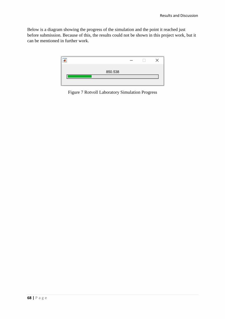
Results and Discussion
68 | P a g e
Below is a diagram showing the progress of the simulation and the point it reached just
before submission. Because of this, the results could not be shown in this project work, but it
can be mentioned in further work.
Figure 7 Rotvoll Laboratory Simulation Progress
Conclusion
69 | P a g e
7 CONCLUSION
This project work has considered the modelling of an adsorption process by building a
Matlab model. This project is a continuation of the previous specialisation project carried out
by the same student in Autumn 2016. The entire work has been done in four parts, in which a
detailed study on the adsorption dehydration process has been considered, as well as models
and tools used to simulate heat and mass transfer in adsorption process. The adsorption
process at the Statoil Rotvoll laboratory has also been described.
A Matlab model has been developed to simulate bed saturation and mass transfer zone, also a
model for heat transfer has also been developed to see the temperature distributions between
the gas, adsorbent and column wall. It should be noted that some ideas in forming this Matlab
code and all the base case simulation parameters were gotten from a previous work by Kjetil
Gamst and he has been referenced appropriately.
The bed saturation model was run and it was observed that different bed saturation lengths
were gotten for different adsorption times in an adsorption cycle. The bed saturation length
was shorter for a shorter adsorption time, and this length increased as the time of adsorption
increased. This is because the longer the time of adsorption is, more gas enters the column
and more water is adsorbed onto the adsorbent. The equilibrium zone therefore increases in
length from the top of the column, pushing the mass transfer zone towards the bottom of the
column. Therefore, it can be concluded that the length of the equilibrium zone during an
adsorption process is a function of how long the adsorption process is run in an adsorption
cycle. The length of the MTZ has been chosen to be constant throughout the adsorption
process, as this was suggested by John Campbell, but in practice the MTZ length is shorter at
the top of the column, but it gets longer towards the exit or bottom of the column
Sensitivity analysis was carried out on feed gas temperature and water saturation to see what
effect these have on the adsorption process. The base case feed gas temperature used in this
project was 27 0C. The feed gas temperature was reduced to 10 0C and increased to 50 0C
with all other parameters kept constant. The maximum and minimum temperature for the
Rotvoll laboratory is -5 and 70 0C, so the temperatures used for sensitivity analysis is within
range. It was observed that when the temperature was 10 0C, the bed loading increased from a
base case value of 38.5% weight to 40% weight. Conversely, when the temperature was 50 0C, the bed loading the bed loading decreased from 38.5% weight to 35.5% weight. In
industrial operations, the temperature of the feed gas is determined by the process upstream
of the adsorption column. There is usually a scrubber upstream of the column, and the
operating temperature of the scrubber determines how much water is knocked out in the
scrubber, thereby determining the amount of water that enters the adsorption column with the
gas. In this simulation, only the feed gas temperature was changed, with the water saturation
kept constant.

Conclusion
70 | P a g e
Sensitivity analysis was also done with the feed gas water saturation to see how it affects the
adsorption process. The base case feed gas water saturation of 730 ppm was reduced to 200
ppm and increased to 930 ppm. At 200 ppm water saturation, the bed loading was 35.0%
weight, and at 930 ppm the bed loading was 39.5% weight. This indicates that the water
saturation of the feed gas affects the bed loading level. Although the water saturation is
determined by the temperature and pressure of the feed gas in practice, this parameter was
specified in building the Matlab model.
A heat transfer model was built and simulated to see the temperature interactions between the
gas, adsorbent and column wall. In industry and normal practice, there is a slight temperature
difference between the gas, adsorbent and wall towards the bottom or exit of the column.
Unfortunately, in this model, this difference was not noticed, rather the gas, adsorbent and
wall temperature all remained 27 0C throughout the column. Even when the heat of
adsorption was increased, this was stull the case. This can be due to several reasons, but the
most probable one could be that the Matlab model was faulty, and therefore the temperature
interactions couldn’t be observed.
The following conclusions can be drawn from the results of this project work;
• The length of the bed saturation, or the equilibrium zone is dependent on the duration
of the adsorption time in an adsorption cycle
• The feed gas temperature determines the amount of water that enters the column, and
this in turn determines the bed loading in an adsorption process
• The feed gas water saturation also determines the amount of water coming into the
column and determines the bed loading
Desorption process has not been considered in this project, the Matlab model was limited to
only adsorption process.
It took a very long time to get the Matlab model up and running correctly. The Matlab model
started to work close to the end of the project work. It was taking a very long time also for the
adsorption rig at the Statoil Rotvoll Laboratory to simulate, and the results were not gotten
before the project submission deadline. Hence the results were not included in this project.

Further Work
71 | P a g e
8 FURTHER WORK
This project has considered the development of a Matlab model to simulate an adsorption
process. A Matlab model has been developed to simulate heat and mass transfer in an
adsorption process, using base case parameters from a previous work by a student.
Because the Matlab code took a long time to start running correctly, there was not enough
time to run simulations of the Rotvoll Laboratory rig. For future work and purposes, the
Rotvoll Laboratory can be simulated with the Matlab code, as a further development.
Also, desorption process has not been considered in this project work. The adsorption code
built can further be developed in the future into a desorption model and then desorption
process can be simulated for a base case and thereafter the Rotvoll Laboratory.
The effects of TEG on an adsorption process has also not be considered in this project work.
The effects of TEG and possible solutions can be investigated in future work, based on the
adsorption model that has been developed in this project work.
References
72 | P a g e
9 REFERENCES
[1] Natgas 2013, ‘Overview of Natural Gas’, Retrieved 15.10.2016, from
http://naturalgas.org/overview/background/.
[2] Spectra Energy, ‘Natural Gas Processing’, Retrieved 15.10.2016, from
http://www.spectraenergy.com/Operations/What-We-Do/We-Process-Transport-
Store-Natural-Gas/.
[3] Olav B., Even S., Jostein P., TEP 4185 Compendium, “Natural Gas Technology”,
Autumn 2015.
[4] Frank L. Slejko, “Adsorption Technology”, Chemical Industries/19.
[5] Christie J. Geankpolis, “Transport Processes and Separation Processes Principles”,
(4th Edition).
[6] Gas Cleaning and Emission Control, TEP 4212 Compendium, Autumn 2016.
[7] Motoyuki Suzuki, “Adsorption Engineering”, Chemical Engineering Monograph.
[8] John M. Campbell, “Gas Conditioning and Processing”, Campbell Petroleum Series.
[9] Douglas M. Ruthven, “Principles of Adsorption and Adsorption Processes”, John
Wiley and Sons.
[10] A. Buekens, N.N. Zyaykina, “Adsorbents and Adsorption Processes for Pollution
Control”.
[11] TEP 08 ‘Gas Processing and LNG’ Compendium, “Dehydration of Gas by
Adsorption”, Fall 2016.
[12] ‘A New Classification of Adsorption Isotherms’, Retrieved 17.10.2016, from
http://www.nigelworks.com/mdd/PDFs/NewClass.pdf.
[13] ‘Adsorption Isotherm’, 2010, Retrieved 17.10.2016, from
http://www.chemistrylearning.com/adsorption-isotherm/.
[14] Ashleigh Fletcher 2008, ‘Isotherms and Adsorption Theory’, Retrieved 17.10.2016,
from http://personal.strath.ac.uk/Ashleigh.Fletcher/isotherms.htm.
[15] ‘Temperature Swing Adsorption (TSA)’, Retrieved 19.10.2016, from
http://www.separationprocesses.com/Adsorption/AD_Chp02b2.htm#TopPage.
[16] ‘Pressure Swing Adsorption (PSA)’, Retrieved 19.10.2016, from
http://www.separationprocesses.com/Adsorption/AD_Chp02b1.htm.
[17] PetroSkills, John M. Campbell, November 2015 Tip of the Month, “Adsorption
Dehydration: Two – Tower vs Three – Tower System”.
[18] PetroSkills, John M. Campbell, October 2015 Tip of the Month, “What is the impact
of Feed Gas Conditions on the Adsorption Dehydration System”.
[19] PetroSkills, John M. Campbell, May 2015 Tip of the Month, “Benefits of Standby
Time in Adsorption Dehydration Process”.

References
73 | P a g e
[20] Prosim Software and Services, ‘Dynamic Adsorption Column Simulation’, Retrieved
20.10.2016, from http://www.prosim.net/en/software-prosim-dac-12.php.
[21] GCAP Software, John M. Campbell, Retrieved on 20.10.16, from
http://www.jmcampbell.com/gcap-software.php.
[22] Yuh – Shan Ho, “Review of Second – Order Models for Adsorption Systems”,
November 2004, Journal of Hazardous Materials, Elsevier.
[23] Zhe XU, Jian – guo CAI, Bing – cai PAN, “Mathematically modelling Fixed – bed
Adsorption in Aqueous Systems”, January 2013, Jzus.
[24] S. Sircar, J.R. Hufton, “Why does the Linear Driving Force Model for Adsorption
Kinetics Work”, August 1999, Kluwer Academic Publishers.
[25] Yu Liu, “New Insights into Pseudo – second – order kinetic equation for Adsorption”,
December 2006, Elsevier.
[26] R. J. Wijngaarden, K. R. Westerterp, “A Heterogeneous Model for Heat Transfer in
Packed Beds”, July 1992, Chemical Engineering Science.
[27] D. Vortmeyer, R. J. Schaefer, “Equivalence of One and Two – Phase Models for Heat
Transfer Processes in Packed Beds: One Dimensional Theory”, May 1973, Chemical
Engineering Science.
[28] Dongsheng Wen, Yulong Din, “Heat Transfer of Gas Flow Through a Packed Bed”,
February 2006, Chemical Engineering Science.
[29] Anthony G. Dixon, “An Improved Equation for the Overall Heat Transfer Coefficient
in Packed Beds”, January 1996, Chemical Engineering and Processing.
[30] Kjetil Gamst, “Experiments and Modelling of Adsorption Process Used for Natural
Gas Dehydration”, June 2013, Master Thesis at NTNU.

Appendix
74 | P a g e
10 Appendix
10.1 Physical Properties of the Inlet Gas
The physical properties of the feedgas such as the thermal conductivity, density and viscosity
were gotten from the Aspen Hysys software. These properties were used in the heat transfer
simulation code. The Peng Robinson equation of state was used as the fluid package and the
composition of the feedgas used is Methane (86.3mol%), Ethane (6.5mol%), Propane
(2.7mol%), Butane (1.2mol%), Nitrogen (2.7 mol%), C5+ (0.6mol%) and water (730 ppm).
The temperature, pressure and flowrate of the feedgas is 25 – 225 oC, 65 bar and 681400 kg/h
respectively.
The table below shows the values gotten from Aspen Hysys.
Temperature, oC Thermal
Conductivity, W/mK
Density, Kg/m3 Viscosity, PaS
25 3.821E-02 59.63 1.322E-05
27 3.840E-02 58.94 1.326E-05
50 4.083E-02 52.24 1.378E-05
75 4.381E-02 46.80 1.440E-05
100 4.705E-02 42.57 1.503E-05
125 5.049E-02 39.16 1.567E-05
150 5.409E-02 36.32 1.630E-05
175 5.783E-02 33.92 1.690E-05
200 6.170E-02 31.85 1.750E-05
225 6.569E-02 30.04 1.809E-05
Table 10.1 Feedgas properties from Aspen Hysys

Appendix
75 | P a g e
Fig 10.1 Thermal conductivity of gas at 65 bar as a function of temperature
Fig 10.2 Density of gas at 65 bar as a function of temperature
0.00E+00
1.00E-02
2.00E-02
3.00E-02
4.00E-02
5.00E-02
6.00E-02
7.00E-02
0 50 100 150 200 250
Ther
mal
Co
nd
uct
ivit
y [W
/mK
]
Temperature [C]
Thermal Conductivity [k] as f(T)
ThermalConductivity, kLinear (ThermalConductivity, k)
0
10
20
30
40
50
60
70
0 50 100 150 200 250
Den
sity
[kg
/m3
]
Temperature [C]
Density as f(T)
Density asf(T)

Appendix
76 | P a g e
Fig 10.3 Temperature of gas at 65 bar as a function of temperature
10.2 Derivation of Heat Transfer Expression
There are different correlations for determining the heat transfer coefficient in packed beds.
The correlation that has been chosen to work with in this project is the Geankoplis’ method.
The development is shown below;
𝑑𝑄 = ℎ(𝑎𝑆𝑑𝑧)(𝑇1 − 𝑇2) 10.1
Where a is the solid particle surface per unit volume of the bed [m-1] and S is the empty
cross-sectional area of the bed [m2], h is the convectional heat transfer coefficient [kJ/m2K]
and T1 and T2 are the temperatures of the gas and the packing respectively.
For heat transfer in a packed bed of spheres and a Reynolds number of 10 – 4000, the
following correlation has been found to be valid;
휀𝐽�̅� = 휀ℎ
𝐶𝑝𝜌𝑉(
𝐶𝑝𝜇
𝑘)𝑓
2/3= 0.4548𝑁𝑅𝑒
−0.4069 10.2
The subscript f indicates that the values are evaluated at the film temperature. The film
temperature is the arithmetic mean temperature between the gas and the solid temperatures.
Cp is the heat capacity of the gas [kJ/kgK], 𝜌 is the density of the gas [kg/m3], 𝜇 is the
viscosity of the gas [Pas], k is the thermal conductivity of the gas [W/mK].
𝑁𝑅𝑒 =𝑑𝑝𝑉𝜌
𝜇𝑓 10.3
0.00E+00
2.00E-06
4.00E-06
6.00E-06
8.00E-06
1.00E-05
1.20E-05
1.40E-05
1.60E-05
1.80E-05
2.00E-05
0 50 100 150 200 250
Vis
cosi
ty [
Pas
]
Temperature [C]
Viscosity as f(T)
Viscosity asf(T)

Appendix
77 | P a g e
V is the superficial velocity of the gas in an empty column.
𝑉 =𝑄𝑚
𝐴=
�̇�
𝜌𝐴=
4�̇�
𝜌𝜋𝐷𝑐2 10.4
�̇� is the mass flow rate [kg/s]. Substituting equation 10.4 into equation 10.3 gives;
𝑁𝑅𝑒 =4𝑑𝑝�̇�
𝜋𝐷𝑐2𝜇𝑓
10.5
𝑑𝑝 is the size of the particles in the bed (1/8’’=0.003175m) and Dc is the inner diameter of the
bed (4.0m).
Solving equation 10.2 for h by using correlations in equations 10.4 and 10.5 gives;
ℎ =4�̇�
𝜌𝜋𝐷𝑐2
𝐶𝑝
𝜀(
𝐶𝑝𝜇
𝑘)
𝑓
−2
30.4548(
4𝑑𝑝�̇�
𝜋𝐷𝑐2𝜇𝑓
)−04069 10.6
Substituting h in equation 10.6 for h in equation 10.1 gives the expression for the heat
transfer between the gas and the adsorbent;
𝑑𝑞 =4�̇�
𝜌𝜋𝐷𝑐2
𝐶𝑝
휀(
𝐶𝑝𝜇
𝑘)
𝑓
−23
0.4548(4𝑑𝑝�̇�
𝜋𝐷𝑐2𝜇𝑓
)−04069
(𝑎𝑆𝑑𝑧)(𝑇1 − 𝑇2) 10.7
휀 = 0.38 for spheres poured into bed 0.375 – 0.391 as suggested by Dullien in 1992.
The surface area per volume of sphere is 6/d and the volume of sphere per volume of column
is (1- 휀). For a given column volume;
𝑎 =𝐴𝑝
𝑉𝑐=
6(1−𝜀)
𝑑𝑝= 1171.65[𝑚−1] 10.8
Where the subscripts p and c mean pellet and column respectively.
Inserting for S, a, 휀 and expressing dQ as a function of temperature gives;
𝒅𝒒(𝑻) = 𝟏𝟒𝟎𝟐. 𝟐𝟖�̇�𝑪𝒑𝒅𝒛 (𝑪𝒑𝝁(𝑻𝒇)
𝒌(𝑻𝒇))
𝒇
−𝟐𝟑
(𝟒𝒅𝒑�̇�
𝝅𝑫𝒄𝟐𝝁𝒇(𝑻𝒇)
)−𝟎𝟒𝟎𝟔𝟗
(𝑻𝟏 − 𝑻𝟐) 10.9
The Reynolds number is given as;
𝑅𝑒𝐷 =𝑉𝑑𝑝
𝜈=
𝑑𝑝𝑉𝜌
𝜇=
4�̇�𝑑𝑝
𝜇𝜋𝐷𝑐2 10.10

Appendix
78 | P a g e
Values Used
The values used in the equations are given below;
a = 1171.65[m-1]
Dc = 4.0m
S = 𝜋𝐷𝑐
2
4 = 12.566m2
�̇� = 681400kg/h
𝜇 = function of temperature (values in appendix 10.1)
K = function of temperature (values in appendix 10.1)
𝑑𝑝 = 1/8’’ = 0.003175m
dz = dy [defined in the Matlab code as column height (H) divided by number of height
sections (ny)]
10.3 Mass Transfer Zone Calculation
John Campbell has suggested a method to estimate the length of the mass transfer zone in a
Molecular Sieve adsorption process. This method is shown below;
ℎ𝑧 = 0.6𝐴 [𝑞𝑤
0.7895
𝑣𝑔0.5506(𝑅.𝑆)0.2646] 10.11
Where
𝐴 = constant
ℎ𝑧 = MTZ length [cm]
𝑞𝑤 = water loading [kg/h.m2]
𝑣𝑔 = superficial velocity of the gas [m/min]
𝑅. 𝑆 = relative saturation of inlet gas [%]
The water loading is given as;
𝑞𝑤 = 0.053 [𝑄𝑊
𝐷𝑐2 ] 10.12

Appendix
79 | P a g e
Where
𝑄 = gas flowrate [106 std m3/d]
𝑊 = gas water content [kg/106 std m3]
𝐷𝑐 = column diameter [m]
The operating conditions chosen for the Matlab code development are gotten from Kjetil
Gamsts’ work and are as follows;
Gas flowrate: 681.4 t/h = 20.48.106 Sm3/d
Gas water saturation: 730 ppm
Gas pressure: 65 bara
Gas temperature: 27 oC
Bed diameter: 4.0 m
The gas composition is as follows:
Methane (86.3mol%), Ethane (6.5mol%), Propane (2.7mol%), Butane (1.2mol%), Nitrogen
(2.7 mol%), C5+ (0.6mol%) and water (730 ppm).
The water content and gas density are gotten from Aspen Hysys with the Peng Robinson
Equation of State.
𝑊 = 558.0 kg/h
𝜌 = 58.94 kg/m3
The water loading calculation is;
𝑞𝑤 = 0.053 [20.482944×558
42 ] = 37.860𝑘𝑔/ℎ. 𝑚2
The superficial gas velocity in an empty column is given by equation 10.4;
𝑣𝑔 =𝑄𝑚
𝐴=
�̇�
𝜌𝐴=
4�̇�
𝜌𝜋𝐷𝑐2
𝑣𝑔 = 4(681400/60)[
𝑘𝑔
𝑚𝑖𝑛]
58.94[𝑘𝑔
𝑚3] 𝜋×42[𝑚2]= 0.256
𝑚
𝑠= 15.33
𝑚
𝑚𝑖𝑛

Appendix
80 | P a g e
The length of the mass transfer zone can then be calculated from equation 10.11
ℎ𝑧 = 0.6×141 [37.8600.7895
15.350.5506×1000.2646] = 98.04𝑐𝑚
Making the length of the mass transfer zone a function of mass flowrate (�̇�)
ℎ𝑧 = 0.6×141 [37.8600.7895
15.350.5506
�̇�[𝑡ℎ
]×1000.2646
] = 98.04𝑐𝑚 10.13
10.4 Matlab Code
10.4.1 Mass Transfer and Bed Saturation
The following Matlab code has been used to model the mass transfer and bed saturation of
the adsorption process, and also this is the code with which the sensitivity analysis was
carried out.
clear all clc format long
%Column d= 4.0; %diameter of column [m] h= 7.0; %height of column - MS layer+ 2x ceramic ball layer, [m] Qmh=681400; %Gas mass flow rate [kg/h] (**) Qm=Qmh/3600 ; %Gas mass flow [kg/s] channeling=0; Channeling=100*channeling; % % part of gas that's
channelingif the effect of channeling (all the way through the column) is
to be investigated
%Defining grids ny=240; %number of height sections discretzed dy=h/ny; %step size in the y-direction tmax=60*100; %[s] Total duration of desorption (**) dt=0.025; % [s] size of timestep (**) nt=tmax/dt; %total number of time steps cA=(pi()*d^2)/4; %cross sectional area of column aA=0.62*cA; %Area the adsobent is filling (poured packing- filling factor
=0.62) fA=cA-aA; %free cross sectional area for the gas to flow
%adsorbent properties hvap=4187; %heat of vaporisation, KJ/kg Cpa=1.07; %heat capacity of adsorbent, kJ/kgK

Appendix
81 | P a g e
densa=720; %[kg/m3]density of adsorbent Tadsinitial=27; %initial temperature of adsorbent (at start of
regeneration) mads= 54400; %[kg]total mass of the adsorbent in the column dma=mads/ny; %kg adsorbent per height segment
% Making the capacity equation P=65*10^2; %System pressure [kPa] (**) Ppa=P*1000; %System pressure in [Pa] - to use in mwsg (Silica Gel) R=8.314; %gas constant
%Constants for Langmuir equation follows CH4C=[348.971 0.542 6.770E-06 13672.210; 348.971 0.542 6.130E-07
20307.220]; H2OC=[-3799.940 18.711 3.580E-07 44140.040;3684.491 -4.450 1.620E-05
45199.990]; C11=CH4C(1,1); C12=CH4C(1,2); C13=CH4C(1,3); C14=CH4C(1,4); C21=CH4C(2,1); C22=CH4C(2,2); C23=CH4C(2,3); C24=CH4C(2,4); H11=H2OC(1,1); H12=H2OC(1,2); H13=H2OC(1,3); H14=H2OC(1,4); H21=H2OC(2,1); H22=H2OC(2,2); H23=H2OC(2,3); H24=H2OC(2,4); %T is in kelvin, but as it is added 273 in the equation, C is used
%Defining MS capacity from Langmuir multicomponent adsorption (Water/C1 -
MS 5A): mwadp=@(YH2O,T) 0.725*((H2OC(1,1)/(T+273)
+H2OC(1,2))*(H2OC(1,3)*exp(H2OC(1,4)/(R*(T+273))))*P*YH2O/... (1+((H2OC(1,3)*exp(H2OC(1,4)/(R*(T+273))))*P*YH2O+(CH4C(1,3)*exp(CH4C(1,4)/
(R*(T+273))))*P*(1-YH2O)))+... (H2OC(2,1)/(T+273)
+H2OC(2,2))*(H2OC(2,3)*exp(H2OC(2,4)/(R*(T+273))))*P*YH2O/(1+((H2OC(2,3)*ex
p(H2OC(2,4)... /(R*(T+273))))*P*YH2O+ (CH4C(2,3)*exp(CH4C(2,4)/(R*(T+273))))*P*(1-
YH2O))))*18.015/1000; funT=@(T) 0.725*((H2OC(1,1)/(T+273)
+H2OC(1,2))*(H2OC(1,3)*exp(H2OC(1,4)/(R*(T+273))))*P*YH2O/(1+((H2OC(1,3)... *exp(H2OC(1,4)/(R*(T+273))))*P*YH2O+(CH4C(1,3)*exp(CH4C(1,4)/(R*(T+273))))*
P*(1-YH2O)))+(H2OC(2,1)/(T+273) +... H2OC(2,2))*(H2OC(2,3)*exp(H2OC(2,4)/(R*(T+273))))*P*YH2O/(1+((H2OC(2,3)*exp
(H2OC(2,4)/(R*(T+273))))*P*YH2O+... (CH4C(2,3)*exp(CH4C(2,4)/(R*(T+273))))*P*(1-YH2O))))*18.015/1000; funT1ppm=@(T) dma*0.725*((H2OC(1,1)/(T+273)
+H2OC(1,2))*(H2OC(1,3)*exp(H2OC(1,4)/(R*(T+273))))*P*10^-6/(1+... ((H2OC(1,3)*exp(H2OC(1,4)/(R*(T+273))))*P*10^-
6+(CH4C(1,3)*exp(CH4C(1,4)/(R*(T+273))))*P*(1-10^-
6)))+(H2OC(2,1)/(T+273)... +H2OC(2,2))*(H2OC(2,3)*exp(H2OC(2,4)/(R*(T+273))))*P*10^-
6/(1+((H2OC(2,3)*exp(H2OC(2,4)/(R*(T+273))))*P*10^-6+... (CH4C(2,3)*exp(CH4C(2,4)/(R*(T+273))))*P*(1-10^-6))))*18.015/1000;
T=27; yi=730*10^-6; %feed gas water content T_initial=T;
%gas properties hfgas=@(xx) (4*10^-6)*(xx)^3 - 0.0007*(xx)^2 +2.6643*(xx) - 66.2325; Mdewf=@(xx) 0.000291*exp(0.039683*xx); %Water content at gas saturation as
function of T Tdewf=@(xx) 25.1997*log(3436.426*xx);%Gas temperature at water saturation
as function of mwg

Appendix
82 | P a g e
Cpg=2.73; %[kJ/kgK] heat capacity og the gas- the value varies very little
with temperature and is therefore sat constant CpgSI=2730; %Cpg in SI units [J/kgK] mwg=zeros(ny,1); %matrix for amount of water in the gas- zero at start of
regeneration mwg1=mwg; %dummy matrix to be used later densgasf=@(tt) 58.94; % [kg/m3] density of the gas as f(Tgas) viscgasf=@(uu) 1.326E-05; %[Pa*s] -viscosity of the gas as f(Tgas) condgasf=@(vv) 3.840E-02; % [W/m2] -thermal conductivity of gas as f(Tgas) Mgasentering=(1-channeling)*Qm*dt; %{kg] amount of gas that enters the
column every timestep Tg=@(xx) (-2.53123*10^-13)*(xx)^5 +(4*10^-10)*(xx)^4 - (3.33*10^-
7)*(xx)^3+(9*10^-5)*(xx)^2 + 0.3745*(xx) + 25; %[C]temperature of gas as a
f(enthalpy) MWgas=18.54; %MW of the gas MWwater=18.02; %MW of water densgasinitial=densgasf(T_initial); densgas=densgasinitial; vginitial=Qm/(fA*densgasinitial); %initial velocity of the gas, m/s
%ceramic ball properties mCpCB=5500*0.84/13; %mCp ceramic balls in one height segment- density is
0.84 kg/m3 and there are 13 height segments
%water properties CpH2O=4.3; %[kJ/kgK] heat capacity of water. this is sat constant both for
liquid and vapor water
%matrices used for calculate the gas movement upwards the column movecells=zeros(ny,1); moveHcells=zeros(ny,1); densgas=zeros(ny,1); movegascells=zeros(ny,1); dtdivdy=dt/dy; %constant to ease code
% Defining initial conditions: Tgas=27*ones(ny,1); %Temperature of gas in column at start of regeneration Hgas=zeros(ny,1); %enthalpy of gas in each segment at start of regeneration Hgas1=Hgas; %dummy matrix Hintot=0; %to track total amount of energy entering the column Tad=27*ones(ny,1);%initial temperature of adsorbent Mgas=zeros(ny,1); %initial amount of gas in column Mgas1=Mgas; %dummy matrix Vg=zeros(ny,1); %initial velocities gas upwards the column Energyout=zeros(ny,1); %to calculate the energy loss to surroundings Energyouttot=zeros(ny,1); %to calculate the total amount of energy lost to
surroundings Energyin=zeros(ny,1); %to track heat transfer from bed to wall Energyintot=zeros(ny,1); %to track total heat transfer from bed to wall free_water=zeros(ny,1); %amount of condensed water in given height segment ppm=0.1*ones(ny,1); %ppm in height segment. minimum ppm =0.1 for capacity
function to be /=0 waterouttime=zeros((tmax/60),1); %tracking amount of gas exiting column
relative to time gasout=0; waterout=0; %tracking amount of gas and water exiting the column
%%%%%%%%CALCULATIONS%%%%%%%
minu=1; waterincounter=0;

Appendix
83 | P a g e
wbar=waitbar(0,'Please wait...'); %waitbar defined
for timestep=1:nt; %timesteps t=dt*timestep; tm=t/60; %t represents time [s] from start, tm [min] Qm=Qmh/3600; %feedgas flowrate is at 100% throughout adsorption
process, kg/s Mgasentering=(1-channeling)*Qm*dt; %{kg] amount of gas that enters the
column every timestep
for j=1:ny; %iteration in the y-direction
%%% GAS/ADSORBTION ITERATIONS %%%
%The Following creates bed saturation as a function of time and
mass transfer zone (0.98m) MTZ_length=0.98; % Length of MTZ in [m] dmwater=mwadp(730*10^-6,27); %[kg] mass of water in adsorbent at
initial conditions mwa=zeros(ny,1); Bed saturation as a fucntion of time for tmax=60*50; %adsorption time of 50 mins mwa(round(5*ny/6 -2):ny)=dma*dmwater; for i=round(5*ny/6 -(MTZ_length*ny/7.0)):round(5*ny/6) sigmoid=(10/(round(5*ny/6)-round(5*ny/6 -
(MTZ_length*ny/7.0)) ))*(i-round(5*ny/6 -(MTZ_length*ny/7.0)) ) -5; mwa(i)=dma*dmwater*(1/(1+exp(-sigmoid))); end end
for tmax=60*100; %adsorption time of 100 mins mwa(round(4*ny/5 -2):ny)=dma*dmwater; for i=round(4*ny/5 -(MTZ_length*ny/7.0)):round(4*ny/5) sigmoid=(10/(round(4*ny/5)-round(4*ny/5 -
(MTZ_length*ny/7.0)) ))*(i-round(4*ny/5 -(MTZ_length*ny/7.0)) ) -5; mwa(i)=dma*dmwater*(1/(1+exp(-sigmoid))); end end % for tmax=60*150; %adsorption time of 150 mins mwa(round(3*ny/4 -2):ny)=dma*dmwater; for i=round(3*ny/4 -(MTZ_length*ny/7.0)):round(3*ny/4) sigmoid=(10/(round(3*ny/4)-round(3*ny/4 -
(MTZ_length*ny/7.0)) ))*(i-round(3*ny/4 -(MTZ_length*ny/7.0)) ) -5; mwa(i)=dma*dmwater*(1/(1+exp(-sigmoid))); end end % % for tmax=60*200; %adsorption time of 200 mins mwa(round(2*ny/3 -2):ny)=dma*dmwater; for i=round(2*ny/3 -(MTZ_length*ny/7.0)):round(2*ny/3) sigmoid=(10/(round(2*ny/3)-round(2*ny/3 -
(MTZ_length*ny/7.0)) ))*(i-round(2*ny/3 -(MTZ_length*ny/7.0)) ) -5; mwa(i)=dma*dmwater*(1/(1+exp(-sigmoid))); end end
for tmax=60*240; %adsorption time of 240 mins mwa(round(1*ny/2 -2):ny)=dma*dmwater;

Appendix
84 | P a g e
for i=round(1*ny/2 -(MTZ_length*ny/7.0)):round(1*ny/2) sigmoid=(10/(round(1*ny/2)-round(1*ny/2 -
(MTZ_length*ny/7.0)) ))*(i-round(1*ny/2 -(MTZ_length*ny/7.0)) ) -5; mwa(i)=dma*dmwater*(1/(1+exp(-sigmoid))); end end
ppm(j)=(10^6*(mwg(j)*MWgas/(Mgas(j)*MWwater))); if isnan(ppm(j))==1 || isinf(ppm(j))==1 || ppm(j)==0 ||ppm(j)<0
%ppm must be >0 (mathematical) ppm(j)=0.1; end
Tf=0.5*(Tgas(j)+Tad(j)); %arithmetic mean temperature of gas and
adsorbent
q1=0.001*dt*dy*1402.28*Qm*CpgSI*((CpgSI*viscgasf(Tf)/condgasf(Tf))^(-
2/3))*... ((2.53*10^-4*Qm/viscgasf(Tf))^(-0.4069))*(Tgas(j)-Tad(j));
%heattransfer between gas and adsorbent from %Geankoplis' relations (0.001 is to convert from J to kJ) qmax=0.92*(Tgas(j)-Tad(j))*(Cpg*Mgas(j)+CpH2O*mwg(j)); %max
theoretical heat transfer possilble (by energy balance) q=min(q1,qmax); %if q1>qmax q must be sat min if q<0 q=max(q1,qmax); end
Tgasj=Tgas(j); Tadj=Tad(j); mwaj=mwa(j); Mgasj=Mgas(j); mwgj=mwg(j); mwadnew=mwa(j); ppmj=ppm(j); if abs(mwgj)<10^-12 mwg(j)=0; mwgj=0; end end
%specifying the inlet gas speed and H value vg(1)=Qm/(fA*densgasinitial); %velocity of gas in the first cell movecells(1)=vginitial*dtdivdy; %size of cell 1 pushed upwards densgas(1)=densgasf(Tgas(1)); %density of gas in first cell
%calculations of gas movements upwards the column
for i=2:ny densgas(i)=densgasf(Tgas(i)); %density of gas in cell i Vg(i)=Qm/(fA*densgas(i-1)); %speed of gas cell i, calculated from
properties of cell below movecells(i)=vg*dtdivdy; %size of cell i that will be pushed upwards
if movecells(i)>1 %if this is the case, you need to check if it might
cause problems display('error, moving more than one cell per timestep')

Appendix
85 | P a g e
return end
movegascells(i)=movecells(i)*Mgas(i); %how much of the mass in cell i
that will move upwards moveHcells(i)=movecells(i)*Hgas(i); %how much of the energy that will
move upwards movemwg(i)=movecells(i)*mwg(i);
end
movegascells(1)=movecells(1)*Mgas(1); %how much of the mass in cell 1
that will move upwards moveHcells(1)=movecells(1)*Hgas(1); %how much of the energy in cell 1
that will move upwards movemwg(1)=movecells(1)*mwg(1);
for i=2:ny
Mgas1(i)=Mgas(i)-movegascells(i)+movegascells(i-1); %mass of the gas
within the cell i after it's shifted Hgas1(i)=Hgas(i)-moveHcells(i)+moveHcells(i-1); %amount of energy in
gas in cell i after it's shifted mwg1(i)=mwg(i)-movemwg(i)+movemwg(i-1); end
Mgasout=Mgas(ny)-movegascells(ny); Hout=Hgas(ny)-moveHcells(ny); waterout=mwg(i);
waterouttime(ceil(minu))=waterouttime(ceil(minu))+waterout; Mgas1(1)=Mgas(1)-movegascells(1)+Mgasentering; %amount of gas in cell
one after it's shifted % Hgas1(1)=Hgas(1)-moveHcells(1)+Hgasentering; %amount of energy in gas
in cell i after it's shifted mwg1(1)=mwg(1)-movemwg(1); Mgas=Mgas1; Hgas=Hgas1; mwg=mwg1; for i=1:ny if Mgas(i)< 0.001*Mgasentering %to avoid dividing by a number close
to zero Tgas(i)=27; else Tgas(i)=27+(Hgas(i)-(mwg(i)*(Tgas(i)-27)*CpH2O))/(Mgas(i)*Cpg); end end
for i=1:ny ppm(i)=(10^6*(mwg(i)*MWgas/(Mgas(i)*MWwater))); if isnan(ppm(i))==1 || isinf(ppm(i))==1 || ppm(i)==0 ppm(i)=0.1; end end
waitbar(t/tmax, wbar, timestep*dt) end %end of timeteps close(wbar)
%creating plot of temperature profiles at t=tend sam=zeros(1,1); %matrix for adsorption, gas and wall temperatures
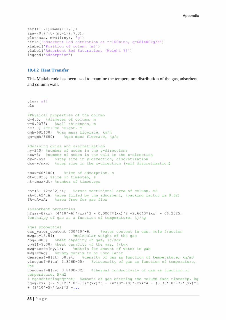
Appendix
86 | P a g e
sam(1:1,1)=mwa(1:1,1); aaa=(0:(7.0/(ny-1)):7.0); plot(aaa, mwa(1:ny), 'g') title('Adsorbent Bed saturation at t=100mins, q=681400kg/h') xlabel('Position of column [m]') ylabel('Adsorbent Bed Saturation, [Weight %]') legend('Adsorption')
10.4.2 Heat Transfer
This Matlab code has been used to examine the temperature distribution of the gas, adsorbent
and column wall.
clear all clc
%Physical properties of the column d=4.0; %diameter of column, m w=0.0078; %wall thickness, m h=7.0; %column height, m qmh=681400; %gas mass flowrate, kg/h qm=qmh/3600; %gas mass flowrate, kg/s
%defining grids and discretization ny=240; %number of nodes in the y-direction; nxw=3; %number of nodes in the wall in the x-direction dy=h/ny; %step size in y-direction, discretization dxw=w/nxw; %step size in the x-direction (wall discretization)
tmax=60*100; %time of adsorption, s dt=0.025; %size of timestep, s nt=tmax/dt; %number of timesteps
cA=(3.142*d^2)/4; %cross sectin\onal area of column, m2 aA=0.62*cA; %area filled by the adsorbent, (packing factor is 0.62) fA=cA-aA; %area free for gas flow
%adsorbent properties hfgas=@(xx) (4*10^-6)*(xx)^3 - 0.0007*(xx)^2 +2.6643*(xx) - 66.2325; %enthalpy of gas as a function of temperature, kj/kg
%gas properties gas_water_content=730*10^-6; %water content in gas, mole fraction mwgas=18.54; %molecular weight of the gas cpg=3000; %heat capacity of gas, kj/kgk cpgSI=3000; %heat capacity of the gas, j/kgk mwg=zeros(ny,1); %matrix for amount of water in gas mwg1=mwg; %dummy matrix to be used later densgasf=@(tt) 58.94; %density of gas as function of temperature, kg/m3 viscgasf=@(uu) 1.326E-05; %viscousity of gas as function of temperature,
PaS condgasf=@(vv) 3.840E-02; %thermal conductivity of gas as function of
temperature, W/m2 % mgasentering=qm*dt; %amount of gas entering the column each timestep, kg tg=@(xx) (-2.53123*10^-13)*(xx)^5 + (4*10^-10)*(xx)^4 - (3.33*10^-7)*(xx)^3
+ (9*10^-5)*(xx)^2 +...

Appendix
87 | P a g e
0.3745*(xx) + 25; %temperature of gas as a function of enthalpy
%water properties cpH2O=4.3; %heat capacity of water, kj/kgk mwwater=18.02; %molecular weight of water
dtdivdy=dt/dy; %constant to ease code
%wall properties cpw=513; %heat capacity of wall, j/kgk kw=15.8; %heat transfer coefficent of wall, W/mk densw=7990; %density of wall material (steel), constant, at 400k hwa=100; %convection heat transfer coefficient, wall/adsorbent, W/m2k
%constant definitions
%wall constants alpha=kw/(densw*cpw); alphax=(alpha*dt)/dxw^2; %must be larger than 0.25, stability reasons alphay=(alpha*dt)/dy^2; %must be larger than 0.25, stability reasons if alphax>0.25 %reports if values gives unstable model display('ALPHAX TOO LARGE') display(alphax); end htx=(hwa*dt)/(dxw*cpw*densw); %consatnt used in wall iteration hxk=hwa*dxw/kw; %constant used in wall iteration
%defining initial conditions tw=27*ones(nxw,ny); %wall temperture matrix tw1=tw; %dummy matrix for wall temperature tgas=27*ones(ny,1); %gas temperature in column at start of regeneration hgas=zeros(ny,1); %enthalpy of gas in each section at start of
regeneration hgas1=hgas; %dummy matrix tad=27*ones(ny,1); %intial temperature of adsorbent mgas=zeros(ny,1); %initial amount of gas in column mgas1=mgas; %dummy matrix
%%%CALCULATIONS%%%
wbar = waitbar(0,'Please wait...'); %defining the waitbar
for timestep=1:nt; %timesteps t=dt*timestep; %t is time from start, s minu=t*dt/60; qm=qmh/3600; %feedgas flowrate, kg/s mgasentering=qm*dt; %amount of gas entering the column each
height section, kg mwgentering=mgasentering*gas_water_content*mwwater/mwgas; %initial
water content of gas
%defining gas inlet properties if t<=tmax %for time of adsorption tgasin=27; densgasinitial=densgasf(tgasin); hgasinitial=hfgas(tgasin); vginitial=qm/(fA*densgasinitial);

Appendix
88 | P a g e
hgasentering=hgasinitial*mgasentering; end
tw=tw1; %dummy matrix (wall temperature at t=n+1, tw is at t=n)
for j=1:ny; %iteration in the y-direction
tw(:,1)=tw(:,2)+(tw(:,2)-tw(:,3));
%%%GAS/ADSORPTION ITERATIONS
tf=0.5*(tgas(j)+tad(j)); %arithmetic mean temperature of gas and
adsorbent q1=0.001*dt*dy*1402.28*qm*cpgSI*((cpgSI*viscgasf(tf)/condgasf(tf))^(-
2/3))*((2.53*10^-4*qm/viscgasf(tf))... ^(-0.4069))*(tgas(j)-tad(j)); %heat transfer between gas and adsorbent
from Geankoplis' relations (0.001 to convert %from j to jk) qmax=0.995*(tgas(j)-tad(j))*(cpg*mgas(j)+cpH2O*mwg(j)); %max
possible theoretical heat transfer (energy balance) q=min(q1,qmax); %if q1>qmax, q must be qmax
if q>0.001 %to avoid iteratons with too small values repeat=1; %variable used to stay in the while-loop while repeat==1; %temperature iterations repeat=0; while tgas(j)-(q/(cpg*mgas(j)+cpH2O*mwg(j)))<tad(j); %if
tgasnew<tad, the q must be reduced q=0.9*((tgas(j)-tad(j))*(cpg*mgas(j)+cpH2O*mwg(j)));
%new, reduced value of q end
tgasnew=tgas(j)-(q/(cpg*mgas(j)+cpH2O*mwg(j))); %new gas
temperature calculated from q C1=dmads*cpa*tad(j)+mwad(j)*(cpH2O*tad(j)-hvap-
cpH2O*tgasnew)+q; %constant tadnew=tad(j)+(tgasnew-tad(j))*0.001; %random guess for new
value of tad(j) error=1; counter=0; counter2=0;
while error>0.0001 %iterations to make the guessed
adsorption values correct mwanew=polyval(mwadp,tadnew); if tgasnew==tad(j) mwanew=mwad(j)-0.005*mwad(j); end
if counter2>50 %to prevent iteration values jumping
between two numbers mwanew=0.8*mwanew2+0.2*mwanew; end
tadnew2=(C1+mwanew*(hvap+cpH2O*tgasnew))/(dmads*cpa+mwanew*cpH2O); mwanew2=0.2*polyval(mwadp,tadnew2)+0.8*mwanew;
Appendix
89 | P a g e
tadnew2=(C1+mwanew2*(hvap+cpH2O*tgasnew))/(dmads*cpa+mwanew*cpH2O); error=abs(tadnew2-tadnew); tadnew=(tadnew2+tadnew)/2; counter=counter+1; counter2=counter2+1;
if counter>200 tadnew=((tadnew+tadnew2)+rand)/2; end
if tadnew<tad(j) tadnew=tad(j)+(tgasnew-tad(j))*0.01*rand; end end %ends while-error
if tadnew>tgasnew || tgasnew>tgas(j) || tadnew<tad(j)
%checking for illogical values q=0.90*q; repeat=1; %repeating itertions display('illogical values') %to check the illogical
values end end %end main iteration while repeat==1
%defining new values deltam=mwad(j)-mwanew2; tgas(j)=tgasnew; tad(j)=tadnew; mwg(j)=mwg(j)+deltam; mwad(j)=mwanew2; hgas(j)=hgas(j)-q+(deltam*cpH2O*(tgas(j)-27)); deltam=0; end %end if q>0.001 end %end 'for' iteration in y-direction
%wall temperatue in top layer of the column tw1(:,ny)=tw(:,ny-1); %boundary condition wall: t unchaged outt
%defining the inlet gas speed and H value vg(1)=qm/(fA*densgasinitial); %gas velocity in first cell, layer,
section movecells(1)=vginitial*dtdivdy; %how big part of cell 1 that will move
upwards densgas(1)=densgasf(tgas(1)); %density of gas in first cell
%calculations of gas movement upwards the column for i=2:ny densgas(i)=densgasf(tgas(i)); %desntiy of gas in cell i vg(i)=qm/(fA*densgas(i-1)); %velocity of gas in cell i movecells(i)=vg(i)*dtdivdy; %how big part of cell i that will
be pushed upwards
if movecells(i)>1 %if so, we check if it might cause problems display('error, moving more than one cell per timestep') return end
movegascells(i)=movecells(i)*mgas(i); %how much mass in cell i
moves upwarsds

Appendix
90 | P a g e
moveHcells(i)=movecells(i)*hgas(i); %how much energy moves
upwards movemwg(i)=movecells(i)*mwg(i);
end
movegascells(1)=movecells(1)*mgas(1); %how much mass in cell 1
moves upwards moveHcells(1)=movecells(1)*hgas(1); %how much energy in cell 1
moves upwards movemwg(1)=movecells(1)*mwg(1);
for i=2:ny
mgas1(i)=mgas(i)-movegascells(i)+movegascells(i-1); %amount of gas
in cell i after it's moved hgas1(i)=hgas(i)-moveHcells(i)+moveHcells(i-1); %amount of
energy in gas in cell i after it's moved mwg1(i)=mwg(i)-movemwg(i)+movemwg(i-1);
end
mgas1(1)=mgas(1)-movegascells(1)+mgasentering; %amount of gas in
cell 1 after it's moved hgas1(1)=hgas(1)-moveHcells(1)+hgasentering; %amount of energy
in gas in cell 1 after it's moved mwg1(1)=mwg(1)-movemwg(1); mgas=mgas1; hgas=hgas1; mwg=mwg1; for i=1:ny if mgas(i)<0.001*mgasentering %to avoid dividing by a number
close to zero tgas(i)=27; else tgas(i)=tg(hgas(i)/mgas(i)); end end
%tgas(120);
%end of gas movement
waitbar(t/tmax, wbar, timestep*dt)
tt=t/600; if ceil(tt) == floor(tt) %creating matrices with temperature
profiles every 10 mins i=t/600; heatdistmatrix(:,1,i)=tgas(:,1); heatdistmatrix(:,2,i)=tad(:,1); heatdistmatrix(:,3,i)=tw(nxw,1:ny); end
minu=t/60; %tracking gas outlet temperatures if ceil(minu) == floor(minu) tout(minu,1)=minu; tout(minu,2)=tgas(ny); end

Appendix
91 | P a g e
end %timestep ends,,,all calculations end at this stage close(wbar) %closes the waitbar
%creating plot of temperature profiles at t=tend l=length(tgas); sam=zeros(1,3); %matrix for adsorption, gas and wall temperatures sam(1:1,1)=tgas(1:1,1); sam(1:1,2)=tad(1:1,1); sam(1:1,3)=tw(nxw,1); minutes=t/60; aaa=(0:(7.0/(ny-1)):7.0); plot(aaa, tw((nxw-1),1:ny), 'r', aaa, tgas(1:ny), 'g', aaa, tad(1:ny), 'b') title(['temperature distribution at ', num2str(minutes),'minutes',',
q=',num2str(qmh), 'kg/h'], 'fontweight','bold') xlabel('Position of column [m]') ylabel('Temperature [C]') legend('Wall','Gas','Adsorbent') axis([0 7.0 0 60])