Improved Deep Learning of Object Category using Pose Information

Jiaping Zhao, Laurent IttiUniversity of Southern California{jiapingz, itti}@usc.edu

Abstract

Despite significant recent progress, the best availablecomputer vision algorithms still lag far behind human capa-bilities, even for recognizing individual discrete objects un-der various poses, illuminations, and backgrounds. Here wepresent a new approach to using object pose information toimprove deep network learning. While existing large-scaledatasets, e.g. ImageNet, do not have pose information, weleverage the newly published turntable dataset, iLab-20M,which has∼22M images of 704 object instances shot underdifferent lightings, camera viewpoints and turntable rota-tions, to do more controlled object recognition experiments.We introduce a new convolutional neural network architec-ture, what/where CNN (2W-CNN), built on a linear-chainfeedforward CNN (e.g., AlexNet), augmented by hierarchi-cal layers regularized by object poses. Pose information isonly used as feedback signal during training, in additionto category information, but is not needed during test. Tovalidate the approach, we train both 2W-CNN and AlexNetusing a fraction of the dataset, and 2W-CNN achieves 6%performance improvement in category prediction. We showmathematically that 2W-CNN has inherent advantages overAlexNet under the stochastic gradient descent (SGD) op-timization procedure. Furthermore, we fine-tune objectrecognition on ImageNet by using the pretrained 2W-CNNand AlexNet features on iLab-20M, results show significantimprovement compared with training AlexNet from scratch.Moreover, fine-tuning 2W-CNN features performs even bet-ter than fine-tuning the pretrained AlexNet features. Theseresults show that pretrained features on iLab-20M gener-alize well to natural image datasets, and 2W-CNN learnsbetter features for object recognition than AlexNet.

1. IntroductionDeep convolutional neural networks (CNNs) have

achieved great success in image classification [14, 25],object detection [21, 8], image segmentation [5], activityrecognition [13, 22] and many others. Typical CNN ar-chitectures, including AlexNet [14] and VGG [23], consist

input

conv1

conv2

conv3

conv4

conv5

fc layers

fc6fc7

object pose object pose

(a) 2W-CNN-I (b) 2W-CNN-MI

Figure 1. 2W-CNN architecture. The orange architecture isAlexNet, and we build two what/where convolutional neural net-work architectures from it: (a) 2W-CNN-I: object pose informa-tion (where) is linked to the top fully connected layer (fc7) only;(b) 2W-CNN-MI: object pose labels have direct pathways to allconvolutional layers. The additionally appended pose architec-tures (green in (a) and blue in (b)) are used in training to regu-larize the deep feature learning process, and in testing, we prunethem and use the remaining AlexNet for object recognition (what).Hence, although feedforward connection arrows are shown, allblue and green connections are only used for backpropagation.

of several stages of convolution, activation and pooling, inwhich pooling subsamples feature maps, making represen-tations locally translation invariant. After several stages ofpooling, the high-level feature representations are invari-ant to object pose over some limited range, which is gen-erally a desirable property. Thus, these CNNs only pre-serve “what” information but discard “where” or pose in-formation through the multiple stages of pooling. However,as argued by Hinton et al. [11], artificial neural networkscould use local “capsules” to encapsulate both “what” and“where” information, instead of using a single scalar tosummarize the activity of a neuron. Neural architecturesdesigned in this way have the potential to disentangle visualentities from their instantiation parameters [19, 32, 9].

In this paper, we propose a new deep architecture builton a traditional ConvNet (AlexNet, VGG), but with two la-bel layers, one for category (what) and one for pose (where;

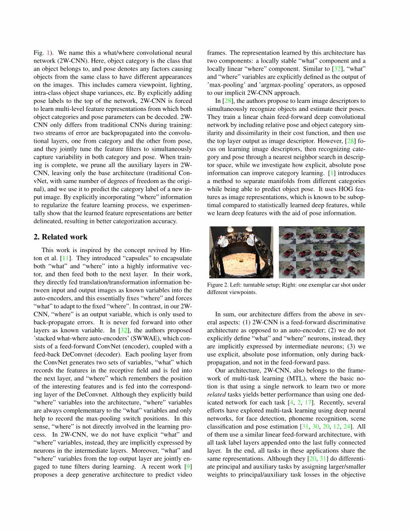
Fig. 1). We name this a what/where convolutional neuralnetwork (2W-CNN). Here, object category is the class thatan object belongs to, and pose denotes any factors causingobjects from the same class to have different appearanceson the images. This includes camera viewpoint, lighting,intra-class object shape variances, etc. By explicitly addingpose labels to the top of the network, 2W-CNN is forcedto learn multi-level feature representations from which bothobject categories and pose parameters can be decoded. 2W-CNN only differs from traditional CNNs during training:two streams of error are backpropagated into the convolu-tional layers, one from category and the other from pose,and they jointly tune the feature filters to simultaneouslycapture variability in both category and pose. When train-ing is complete, we prune all the auxiliary layers in 2W-CNN, leaving only the base architecture (traditional Con-vNet, with same number of degrees of freedom as the origi-nal), and we use it to predict the category label of a new in-put image. By explicitly incorporating “where” informationto regularize the feature learning process, we experimen-tally show that the learned feature representations are betterdelineated, resulting in better categorization accuracy.

2. Related workThis work is inspired by the concept revived by Hin-

ton et al. [11]. They introduced “capsules” to encapsulateboth “what” and “where” into a highly informative vec-tor, and then feed both to the next layer. In their work,they directly fed translation/transformation information be-tween input and output images as known variables into theauto-encoders, and this essentially fixes “where” and forces“what” to adapt to the fixed “where”. In contrast, in our 2W-CNN, “where” is an output variable, which is only used toback-propagate errors. It is never fed forward into otherlayers as known variable. In [32], the authors proposed’stacked what-where auto-encoders’ (SWWAE), which con-sists of a feed-forward ConvNet (encoder), coupled with afeed-back DeConvnet (decoder). Each pooling layer fromthe ConvNet generates two sets of variables, “what” whichrecords the features in the receptive field and is fed intothe next layer, and “where” which remembers the positionof the interesting features and is fed into the correspond-ing layer of the DeConvnet. Although they explicitly build“where” variables into the architecture, “where” variablesare always complementary to the “what” variables and onlyhelp to record the max-pooling switch positions. In thissense, “where” is not directly involved in the learning pro-cess. In 2W-CNN, we do not have explicit “what” and“where” variables, instead, they are implicitly expressed byneurons in the intermediate layers. Moreover, “what” and“where” variables from the top output layer are jointly en-gaged to tune filters during learning. A recent work [9]proposes a deep generative architecture to predict video

frames. The representation learned by this architecture hastwo components: a locally stable “what” component and alocally linear “where” component. Similar to [32], “what”and “where” variables are explicitly defined as the output of’max-pooling’ and ’argmax-pooling’ operators, as opposedto our implicit 2W-CNN approach.

In [28], the authors propose to learn image descriptors tosimultaneously recognize objects and estimate their poses.They train a linear chain feed-forward deep convolutionalnetwork by including relative pose and object category sim-ilarity and dissimilarity in their cost function, and then usethe top layer output as image descriptor. However, [28] fo-cus on learning image descriptors, then recognizing cate-gory and pose through a nearest neighbor search in descrip-tor space, while we investigate how explicit, absolute poseinformation can improve category learning. [1] introducesa method to separate manifolds from different categorieswhile being able to predict object pose. It uses HOG fea-tures as image representations, which is known to be subop-timal compared to statistically learned deep features, whilewe learn deep features with the aid of pose information.

Figure 2. Left: turntable setup; Right: one exemplar car shot underdifferent viewpoints.

In sum, our architecture differs from the above in sev-eral aspects: (1) 2W-CNN is a feed-forward discriminativearchitecture as opposed to an auto-encoder; (2) we do notexplicitly define “what” and “where” neurons, instead, theyare implicitly expressed by intermediate neurons; (3) weuse explicit, absolute pose information, only during back-propagation, and not in the feed-forward pass.

Our architecture, 2W-CNN, also belongs to the frame-work of multi-task learning (MTL), where the basic no-tion is that using a single network to learn two or morerelated tasks yields better performance than using one ded-icated network for each task [4, 2, 17]. Recently, severalefforts have explored multi-task learning using deep neuralnetworks, for face detection, phoneme recognition, sceneclassification and pose estimation [31, 30, 20, 12, 24]. Allof them use a similar linear feed-forward architecture, withall task label layers appended onto the last fully connectedlayer. In the end, all tasks in these applications share thesame representations. Although they [20, 31] do differenti-ate principal and auxiliary tasks by assigning larger/smallerweights to principal/auxiliary task losses in the objective

function, they never make a distinction of tasks when de-signing the deep architecture. Our architecture, 2W-CNN-I(see 4.1 for definition), is similar to theirs, however, 2W-CNN-MI (see 4.1 for definition) is very different: pose isthe auxiliary task, and it is designed to support the learningof the principal task (object recognition) at multiple levels.Concretely, auxiliary labels (pose) have direct pathways toall convolutional layers, such that features in the intermedi-ate layers can be directly regularized by the auxiliary task.We experimentally show that 2W-CNN-MI, which embod-ies a new kind of multi-task learning, is superior to 2W-CNN-I for object recognition, and this indicates that 2W-CNN-MI is advantageous to the previously published deepmulti-task learning architectures.

3. A brief introduction of the iLab-20M datasetiLab-20M [3] was collected by hypothesizing that trainingcan be greatly improved by using many different views ofdifferent instances of objects in a number of categories, shotin many different environments, and with pose informationexplicitly known. Indeed, biological systems can rely onobject persistence and active vision to obtain many differentviews of a new physical object. In monkeys, this is believedto be exploited by the neural representation [16], though theexact mechanism remains poorly understood.

iLab-20M is a turntable dataset, with settings as follows:the turntable consists of a 14”-diameter circular plate ac-tuated by a robotic servo mechanism. A CNC-machinedsemi-circular arch (radius 8.5”) holds 11 Logitech C910USB webcams which capture color images of the objectsplaced on the turntable. A micro-controller system actu-ates the rotation servo mechanism and switches on and off4 LED lightbulbs. Lights are controlled independently, in 5conditions: all lights on, or one of the 4 lights on.

Objects were mainly Micro Machines toys (GaloobCorp.) and N-scale model train toys. These objects presentthe advantage of small scale, yet demonstrate a high levelof detail and, most remarkably, a wide range of shapes (i.e.,many different molds were used to create the objects, asopposed to just a few molds and many different paintingschemes). Backgrounds were 125 color printouts of satel-lite imagery from the Internet. Every object was shot onat least 14 backgrounds, in a relevant context (e.g., cars onroads, trains on railtracks, boats on water).

In total, 1,320 images were captured for each object andbackground combination: 11 azimuth angles (from the 11cameras), 8 turntable rotation angles, 5 lighting conditions,and 3 focus values (-3, 0, and +3 from the default focusvalue of each camera). Each image was saved with loss-less PNG compression (∼1 MB per image). The com-plete dataset hence consists of 704 object instances (15 cat-egories), each shot on 14 or more backgrounds, with 1,320images per object/background combination, or almost 22M

images. The dataset is freely available and distributed onseveral hard drives. One exemplar car instance shot underdifferent viewpoints are shown in Fig. 2(right).

4. Network Architecture and its Optimization

In this section, we introduce our new architecture, 2W-CNN, and some properties of its critical points achievedunder the stochastic gradient descent (SGD) optimization.

4.1. Architecture

Our architecture, 2W-CNN, can be built on any of theCNNs, and, here, without loss of generality, we use AlexNet[14] (but see Supplementary Materials for results usingVGG as well). iLab-20M has detailed pose information foreach image. In the testing presented here, we only consider10 categories, and the 8 turntable rotations and 11 cameraazimuth angles, i.e., 88 discrete poses. It would be straight-forward to use more categories and take light source, focus,etc. into account as well.

Our building base, AlexNet, is adapted here to be suit-able for our dataset: two changes are made, compared toAlexNet in [14] (1) we change the number of units on fc6and fc7 from 4096 to 1024, since we only have ten cate-gories here; (2) we append a batch normalization layer aftereach convolution layer (see the supplementary materials forarchitecture specifications).

We design two variants of our approach: (1) 2W-CNN-I(with I for injection), a what/where CNN with both poseand category information injected into the top fully con-nected layer; (2) 2W-CNN-MI (multi-layer injection), awhat/where CNN with category still injected at the top,but pose injected into the top and also directly into all 5convolutional layers. Our motivation for multiple injectionis as follows: it is generally believed that in CNNs, low-and mid-level features are learned mostly in lower layers,while, with increasing depth, more abstract high-level fea-tures are learned [29, 33]. Thus, we reasoned that detailedpose information might also be used differently by differentlayers. “Multi-layer injection” in 2W-CNN-MI is similarto skip connections in neural networks. Skip connectionis a more generic terminology, while 2W-CNN-MI uses aspecific pattern of skip connections designed specifically tomake pose errors directly back propagate into lower layers.Our architecture details are as follows.2W-CNN-I is built on AlexNet, and we further append apose layer (88 neurons) to fc7. The architecture is shownin Fig. 1. 2W-CNN-I is trained to predict both what andwhere. We treat both prediction tasks as classification prob-lems, and use softmax regression to define the individualloss. The total loss is the weighted sum of individual losses:

L = L(object) + λL(pose) (1)

where λ is a balancing factor, set to 1 in experiments. Al-though we do not have explicit what and where neuronsin 2W-CNN-I, feature representations (neuron responses)at fc7 are trained such that both object category (what)and pose information (where) can be decoded; therefore,neurons in fc7 can be seen to have implicitly encodedwhat/where information. Similarly, neurons in intermedi-ate layers also implicitly encapsulate what and where, sinceboth pose and category errors at the top are back-propagatedconsecutively into all layers, and features learned in the lowlayers are adapted to both what and where.2W-CNN-MI is built on AlexNet as well, but in this variantwe add direct pathways from each convolutional layer to thepose layer, such that feature learning at each convolutionallayer is directly affected by pose errors (Fig. 1). Concretely,we append two fully connected layers to each convolutionallayer, including pool1, pool2, conv3 and conv4, and thenadd a path from the 2nd fully connected layer to the posecategory layer. Fully connected layers appended to pool1and pool2 have 512 neurons and those appended to conv3and conv4 have 1024 neurons. At last, we directly add apathway from fc7 to the pose label layer. The reason we donot append two additional fully connected layers to pool5 isthat the original AlexNet already has fc6 and fc7 on top ofpool5; thus, our fc6 and fc7 are shared by the object cate-gory layer and the pose layer.

The loss function of 2W-CNN-MI is the same as that ofof 2W-CNN-I (Eq. 1). In 2W-CNN-MI, activations from 5layers, namely pool1fc2, pool2fc2, conv3fc2, conv4fc2 andfc7, are all fed into the pose label layer, and responses atthe pose layer are the accumulated activations from all 5pathways, i.e.,

a(LP ) =∑l

a(l) · Wl−LP(2)

where l is one from those 5 layers, Wl−LPis the weight

matrix between l and pose label layer LP , and a(l) are fea-ture activations at layer l.

4.2. Optimization

We use stochastic gradient descent (SGD) to minimizethe loss function. In practice, it either finds a local optimumor a saddle point [6, 18] for non-convex optimization prob-lems. How to escape a saddle point or reach a better localoptimum is beyond the scope of our work here. Since both2W-CNN and AlexNet are optimized using SGD, readersmay worry that object recognition performance differencesbetween 2W-CNN and AlexNet might be just occasionaland depending on initializations, while here we show theo-retically that it is easier to find a better critical point in theparameter space of 2W-CNN than in the parameter space ofAlexNet by using SGD.

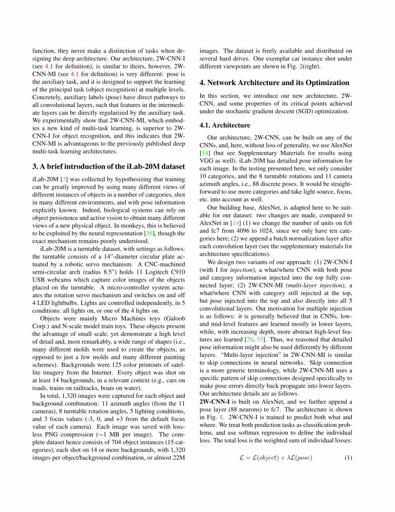
We prove that, in practice, a critical point of AlexNetis not a critical point of 2W-CNN, while a critical point of

object pose

X1

X0

X2 X3

ω2

ω1

ω0

ω3

input

Figure 3. A simplified CNN used in proof.

2W-CNN is a critical point of AlexNet as well. Thus, if weinitialize weights in a 2W-CNN from a trained AlexNet (i.e.,we initialize ω1, ω2 from the trained AlexNet, while initial-izing ω3 by random Gaussian matrices in Fig. 3), and con-tinue training 2W-CNN by SGD, parameter solutions willgradually step away from the initial point and reach a new(better) critical point. However, if we initialize parametersin AlexNet from a trained 2W-CNN and continue training,the parameter gradients in AlexNet at the initial point are al-ready near zero and no better critical point is found. Indeed,in the next section we verify this experimentally.

Let L = f(ω1, ω2) and L̂ = f(ω1, ω2) + g(ω1, ω3) bethe softmax loss functions of AlexNet and 2W-CNN respec-tively, where f(ω1, ω2) in L and L̂ are exactly the same, weshow in practical cases that: (1) if (ω′1, ω

′2) is a critical point

of L, then (ω′1, ω′2, ω3) is not a critical point of L̂; (2) on the

contrary, if (ω′′1 , ω′′2 , ω

′′3 ) is a critical point of L̂, (ω′′1 , ω

′′2 ) is

a critical point of L as well. Here we prove (1) but refer thereaders to the supplementary materials for the proof of (2).

∂L∂ω′

1= ∂f

∂ω′1=−→0

∂L∂ω′

2= ∂f

∂ω′2=−→0

}

∂L̂∂ω′

1= ∂f

∂ω′1+ ∂g

∂ω′16= −→0

∂L̂∂ω′

2= ∂f

∂ω′2=−→0

∂L̂∂ω3

= ∂g∂ω36= −→0

(3)Proof: assume there is at least one non-zero entry inx1 ∈ R1024 (in practice x1 6=

−→0 , x0 6=

−→0 , at least

one non-zero entry, see supplementary materials), and letxnz1 be that non-zero element (nz is its index, nz ∈{1, 2, ..., 1024}). Without loss of generality, we initialize allentries in ω3 ∈ R88×1024 be to 0, except one entry ωnz,1

3 ,which is the weight between xnz1 and x13. Since we havex3 = ω3x1, (x3 = R88), then x13 = ωnz,1

3 · xnz1 6= 0, whilexi3 = 0 (i 6= 1).

In the case of softmax regression, we have: ∂L̂∂xc

3= 1 −

exc3/

∑i e

xi3 ; ∂L̂

∂xi3= −exi

3/∑

i exi3 when i 6= c, where xi3

is the ith entry in the vector x3, and c is the index of theground truth pose label. Since x13 6= 0 and xi3 = 0(i 6=1), ∂L̂

∂xi36= 0 (i ∈ {1, 2, ..., 88}). By chain rule, we have

∂L̂∂ωmn

3= ∂L̂

∂xn3· ∂xn

3

∂ωmn3

= ∂L̂∂xn

3· xm1 , and therefore, as long

as not all entries in x1 are 0, i.e., x1 6=−→0 , we have ∂L̂

∂ω3=

∂L̂∂x3· x1 6=

−→0 .

To show ∂L̂∂ω′

1= ∂f

∂ω′1+ ∂g

∂ω′16= −→0 , we only have to show

∂g∂ω′

16= −→0 (since ∂f

∂ω′1=−→0 ). By chain rule, we have ∂g

∂ω′1=

∂g∂x1· ∂x1

∂ω′1

, where ∂g∂xi

1= 0, when i 6= nz; ∂g

∂xnz1

= ωnz,13 −

ωnz,13 · ex1

3/∑

i exi3 6= 0. Let the weight matrix between

x0 and x1 be ω′0, and by definition, ω′0 ∈ ω′1. Now wehave ∂xnz

1

∂ω′06= −→0 , otherwise x0 =

−→0 . Therefore ∂g

∂ω′1=

∂g∂x1· ∂x1

∂ω′16= −→0 , since ∂g

∂x16= −→0 and ∂x1

∂ω′16= −→0 .

However, a critical point of 2W-CNN is a critical pointof AlexNet, i.e., Eq. 4, see supplementary materials for theproof, and next section for experimental validation.

∂L̂∂ω′′

1= ∂f

∂ω′′1+ ∂g

∂ω′′1=−→0

∂L̂∂ω′′

2= ∂f

∂ω′′2=−→0

∂L̂∂ω′′

3= ∂g

∂ω′′3=−→0

{

∂L∂ω′′

1= ∂f

∂ω′′1=−→0

∂L∂ω′′

2= ∂f

∂ω′′2=−→0

(4)

5. ExperimentsIn experiments, we demonstrate the effectiveness of 2W-

CNN for object recognition against linear-chain deep archi-tectures (e.g., AlexNet) using the iLab-20M dataset. We doboth quantitative comparisons and qualitative evaluations.Further more, to show the learned features on iLab-20M areuseful for generic object recognitions, we adop the “pretrain- fine-tuning” paradigm, and fine tune object recognition onthe ImageNet dataset [7] using the pretrained AlexNet and2W-CNN-MI features on the iLab-20M dataset.

5.1. Dataset setup

Object categories: we use 10 (out of 15) categories of ob-jects in our experiments (Fig. 6), and, within each category,we randomly use 3/4 instances as training data, and the re-maining 1/4 instances for testing. Under this partition, in-stances in test are never seen during training, which mini-mizes the overlap between training and testing.Pose: here we take images shot under one fixed light source(with all 4 lights on) and camera focus (focus = 1), but all11 camera azimuths and all 8 turntable rotations (88 poses).

We end up with 0.65M (654,929) images in the trainingset and 0.22M (217,877) in the test set. Each image is asso-ciated with 1 (out of 10) object category label and 1 (out of88) pose label.

5.2. CNNs setup

We train 3 CNNs, AlexNet, 2W-CNN-I and 2W-CNN-MI, and compare their performances on object recognition.We use the same initialization for their common param-eters: we first initialize AlexNet with random Gaussianweights, and re-use these weights to initialize the AlexNetcomponent in 2W-CNN-I and 2W-CNN-MI. We then ran-domly initialize the additional parameters in 2W-CNN-I /2W-CNN-MI.

No data augmentation: to train AlexNet for object recog-nition, in practice, one often takes random crops and alsohorizontally flips each image to augment the training set.However, to train 2W-CNN-I and 2W-CNN-MI, we couldtake random crops but we should not horizontally flip im-ages, since flipping creates a new unknown pose. For a faircomparison, we do not augment the training set, such thatall 3 CNNs use the same amounts of images for training.

Optimization settings: we run SGD to minimize the lossfunction, but use different starting learning and dropoutrates for different CNNs. AlexNet and 2W-CNN-I havesimilar amounts of parameters, while 2W-CNN-MI has 15times more parameters during training (but remember thatall three models have the exact same number of parame-ters during test). To control overfitting, we use a smallerstarting learning rate (0.001) and a higher dropout rate (0.7)for 2W-CNN-MI, while for AlexNet and 2W-CNN-I, we setthe starting learning rate and dropout rate to be 0.01 and 0.5.Each network is trained for 30 epochs, and approximately150,000 iterations. To further avoid any training setup dif-ferences, within each training epoch, we fix the image or-der. We train CNNs using the publicly available Matconvnet[27] toolkit on a Nvidia Tesla K40 GPU.

5.3. Performance evaluation

In this section, we evaluate object recognition perfor-mance of the 3 CNNs. As mentioned, for both 2W-CNN-Iand 2W-CNN-MI, object pose information is only used intraining, but the associated machinery is pruned away be-fore test (Fig. 1).

Since all three architectures are trained by SGD, the solu-tions depend on initializations. To alleviate the randomnessof SGD, we run SGD under different initializations and re-port the mean accuracy. We repeat the training of 3 CNNsunder 5 different initializations, and report their mean accu-racies and standard deviations in Table 1. Our main result is:(1) 2W-CNN-MI and 2W-CNN-I outperform AlexNet by6% and 5%; (2) 2W-CNN-MI further improves the accuracyby 1% compared with 2W-CNN-I. This shows that, underthe regularization of additional pose information, 2W-CNNlearns better deep features for object recognition.

AlexNet 2W-CNN-I 2W-CNN-MI

accuracy0.785

(±0.0019)0.837

(±0.0022)0.848

(±0.0031)mAP 0.787 0.833 0.850

Table 1. Object recognition performances of AlexNet, 2W-CNN-Iand 2W-CNN-MI on iLab-20M dataset. 2W-CNN-MI performedsignificantly better than AlexNet (t-test, p < 1.6 · 10−5), and 2W-CNN-I (p < 6.3 · 10−5) as well. 2W-CNN-MI was also signifi-cantly better than 2W-CNN-I (p < .013).

As proven in Sec. 4.2, in practice a critical point of

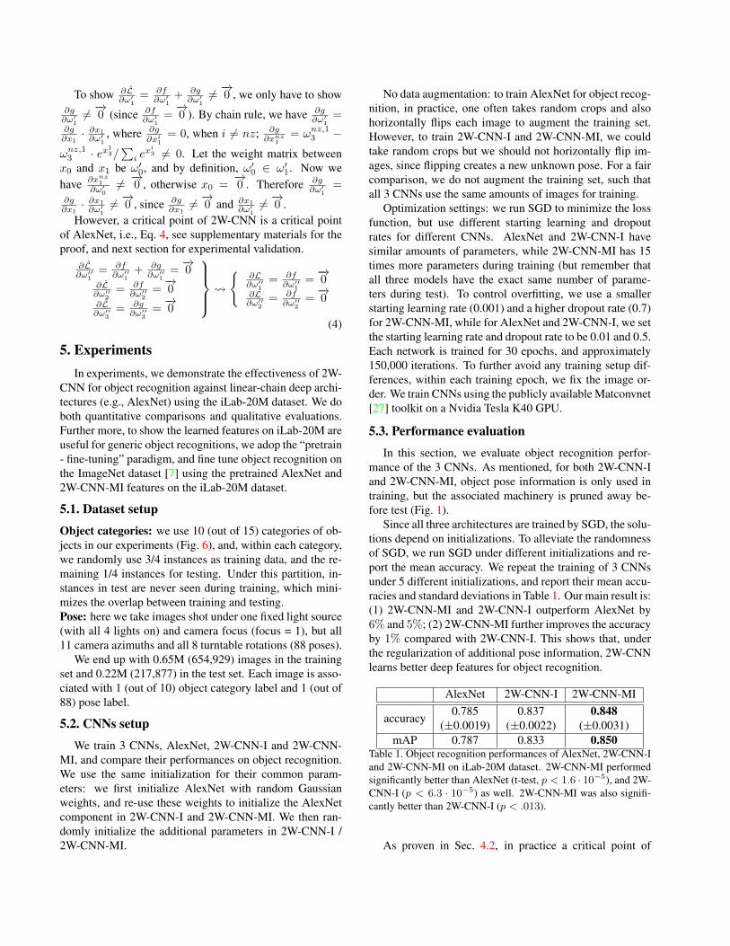
AlexNet is not a critical point of 2W-CNN, while a criticalpoint of 2W-CNN is a critical point of AlexNet. We verifycritical points of two networks using experiments: (1) weuse the trained AlexNet parameters to initialize 2W-CNN,and run SGD to continue training 2W-CNN; (2) conversely,we initialize AlexNet from the trained 2W-CNN and con-tinue training for some epochs. We plot the object recogni-tion error rates on test data against training epochs in Fig. 4.As shown, 2W-CNN obviously reaches a new and bettercritical point distinct from the initialization, while AlexNetstays around the same error rate as the initialization.

1 3 5 7 9 11 13

0.15

0.16

0.17

0.18

0.19

0.2

0.21

0.22

0.23

training epoch

test err

or

rate

trained 2W−CNN−MI

alexnet: initialized from 2W−CNN−MI

trained alexnet

2W−CNN−MI: initialized from alexnet

Figure 4. Critical points of CNNs. We initialize one network fromthe trained other network, continue training, and record test errorsafter each epoch. Starting from a critical point of AlexNet, 2W-CNN-MI steps away from it and reaches a new and better criticalpoint, while AlexNet initialized from 2W-CNN-MI fails to furtherimprove on test performance.

5.4. Decoupling of what and where

2W-CNNs are trained to predict what and where. Al-though 2W-CNNs do not have explicit what and where neu-rons, we experimentally show that what and where informa-tion is implicitly expressed by neurons in different layers.

One might speculate that in 2W-CNN, more than in stan-dard AlexNet, different units in the same layer might be-come either pose-defining or identity-defining. A pose-defining unit should be sensitive to pose, but invariant toobject identity, and conversely. To quantify this, we use en-tropy to measure the uncertainty of each unit to pose andidentity. We estimate pose and identity entropies of eachunit as follows: we use all test images as inputs, and we cal-culate the activation (ai) of each image for that unit. Thenwe compute histogram distributions of activations againstobject category (10 categories in our case) and pose (88poses), and let two distributions be Pobj and Ppos respec-tively. The entropies of these two distributions, E (Pobj)and E (Ppos), are defined to be the object and pose uncer-

tainty of that unit. For units to be pose-defining or identity-defining, one entropy should be low and the other high,while for units with identity and pose coupled together, bothentropies are high.

Assume there are n units on some layer l (e.g., 256units on pool5), each with identity and pose entropyE i(obj) and E i(pos) (i ∈ {1, 2, ..., n}), and we or-ganize n identity entropies into a vector E (obj) =[E 1(obj),E 2(obj), ...,E n(obj)] and n pose entropies intoa vector E (pos) = [E 1(pos),E 2(pos), ...,E n(pos)]. If nunits are pose/identity decoupled, then E (obj) and E (pos)are expected to be negatively correlated. Concretely, forentries at their corresponding locations, if one is large, theother is desirable to be small. We define the correlationcoefficient in Eq. 5 between E (obj) and E (pos) to be thedecouple-ness of n units on the layer l, more negative it is,the better units are pose/identity decoupled.

γ = corrcoef (E (obj),E (pose)) (5)

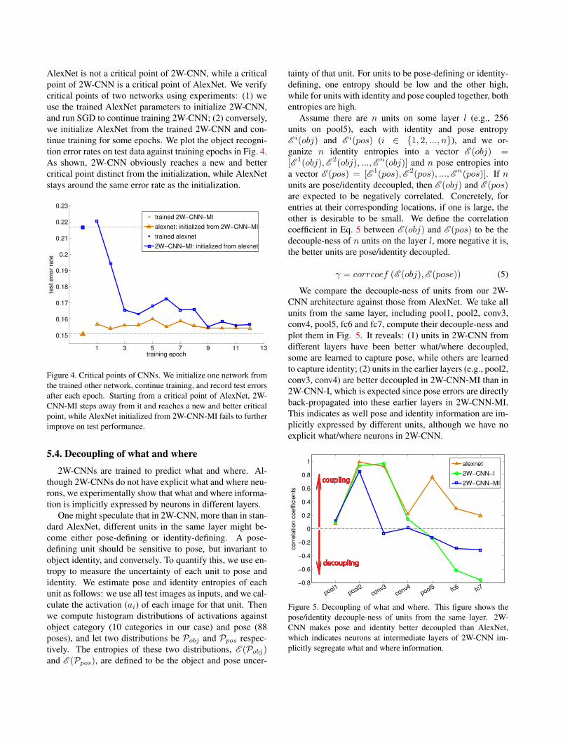
We compare the decouple-ness of units from our 2W-CNN architecture against those from AlexNet. We take allunits from the same layer, including pool1, pool2, conv3,conv4, pool5, fc6 and fc7, compute their decouple-ness andplot them in Fig. 5. It reveals: (1) units in 2W-CNN fromdifferent layers have been better what/where decoupled,some are learned to capture pose, while others are learnedto capture identity; (2) units in the earlier layers (e.g., pool2,conv3, conv4) are better decoupled in 2W-CNN-MI than in2W-CNN-I, which is expected since pose errors are directlyback-propagated into these earlier layers in 2W-CNN-MI.This indicates as well pose and identity information are im-plicitly expressed by different units, although we have noexplicit what/where neurons in 2W-CNN.

−0.8

−0.6

−0.4

−0.2

0

0.2

0.4

0.6

0.8

1

co

rre

latio

n c

oe

ffic

ien

ts

pool1pool2

conv3conv4

pool5 fc6 fc7

alexnet

2W−CNN−I

2W−CNN−MIcoupling

decoupling

coupling

decoupling

coupling

decoupling

coupling

decoupling

coupling

decoupling

Figure 5. Decoupling of what and where. This figure shows thepose/identity decouple-ness of units from the same layer. 2W-CNN makes pose and identity better decoupled than AlexNet,which indicates neurons at intermediate layers of 2W-CNN im-plicitly segregate what and where information.

5.5. Feature visualizations

car

f1car

helicoper

military

monster

pickup

plane

semi

tank

van

2W-CNN-MIalexnet

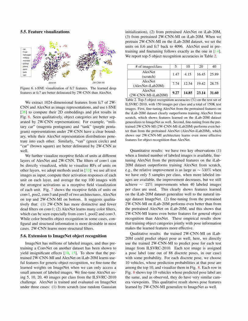
Figure 6. t-SNE visualization of fc7 features. The learned deepfeatures at fc7 are better delineated by 2W-CNN than AlexNet.

We extract 1024-dimensional features from fc7 of 2W-CNN and AlexNet as image representations, and use t-SNE[26] to compute their 2D embeddings and plot results inFig. 6. Seen qualitatively, object categories are better sep-arated by 2W-CNN representations: For example, “mili-tary car” (magenta pentagram) and “tank” (purple penta-gram) representations under 2W-CNN have a clear bound-ary, while their AlexNet representation distributions pene-trate into each other. Similarly, “van” (green circle) and“car” (brown square) are better delineated by 2W-CNN aswell.

We further visualize receptive fields of units at differentlayers of AlexNet and 2W-CNN. The filters of conv1 canbe directly visualized, while to visualize RFs of units onother layers, we adopt methods used in [33]: we use all testimages as input, compute their activation responses of eachunit on each layer, and average the top 100 images withthe strongest activations as a receptive field visualizationof each unit. Fig. 7 shows the receptive fields of units onconv1, poo2, conv3 and pool5 of two architectures, AlexNeton top and 2W-CNN-MI on bottom. It suggests qualita-tively that: (1) 2W-CNN has more distinctive and fewerdead filters on conv1; (2) AlexNet learns many color filters,which can be seen especially from conv1, pool2 and conv3.While color benefits object recognition in some cases, con-figural and structural information is more desirable in mostcases. 2W-CNN learns more structural filters.

5.6. Extension to ImageNet object recognition

ImageNet has millions of labeled images, and thus pre-training a ConvNet on another dataset has been shown toyield insignificant effects [10, 15]. To show that the pre-trained 2W-CNN-MI and AlexNet on iLab-20M learns use-ful features for generic object recognition, we fine-tune thelearned weights on ImageNet when we can only access asmall amount of labeled images. We fine-tune AlexNet us-ing 5, 10, 20, 40 images per class from the ILSVRC-2010challenge. AlexNet is trained and evaluated on ImageNetunder three cases: (1) from scratch (use random Gaussian

initialization), (2) from pretrained AlexNet on iLab-20M,(3) from pretrained 2W-CNN-MI on iLab-20M. When wepretrain 2W-CNN-MI on the iLab-20M dataset, we set theunits on fc6 and fc7 back to 4096. AlexNet used in pre-training and finetuning follows exactly as the one in [14].We report top-5 object recognition accuracies in Table 2.

# of images/class 5 10 20 40AlexNet(scratch) 1.47 4.15 16.45 25.89

AlexNet(AlexNet-iLab20M) 7.74 12.54 19.42 28.75

AlexNet(2W-CNN-MI-iLab20M) 9.27 14.85 23.14 31.60

Table 2. Top-5 object recognition accuracies (%) on the test set ofILSVRC-2010, with 150 images per class and a total of 150K testimages. First, fine-tuning AlexNet from the pretrained features onthe iLab-20M dataset clearly outperforms training AlexNet fromscratch, which shows features learned on the iLab-20M datasetgeneralizes to ImageNet as well. Second, fine-tuning from the pre-trained 2W-CNN-MI (2W-CNN-MI-iLab20M) performs even bet-ter than from the pretrained AlexNet (AlexNet-iLab20M), whichshows our 2W-CNN-MI architecture learns even more effectivefeatures for object recognition than AlexNet.

Quantitative results: we have two key observations (1)when a limited number of labeled images is available, fine-tuning AlexNet from the pretrained features on the iLab-20M dataset outperforms training AlexNet from scratch,e.g., the relative improvement is as large as ∼ 530% whenwe have only 5 samples per class, when more labeled im-ages are available, the improvement decreases, but we stillachieve ∼ 22% improvements when 40 labeled imagesper class are used. This clearly shows features learnedon the iLab-20M dataset generalize well to the natural im-age dataset ImageNet. (2) fine-tuning from the pretrained2W-CNN-MI on iLab-20M performs even better than fromthe pretrained AlexNet on iLab-20M, and this shows that2W-CNN-MI learns even better features for general objectrecognition than AlexNet. These empirical results showthat training object categories jointly with pose informationmakes the learned features more effective.

Qualitative results: the trained 2W-CNN-MI on iLab-20M could predict object pose as well; here, we directlyuse the trained 2W-CNN-MI to predict pose for each testimage from ILSVRC-2010. Each test image is assigneda pose label (one out of 88 discrete poses, in our case)with some probability. For each discrete pose, we choose10 vehicles, whose prediction probabilities at that pose areamong the top 10, and visualize them in Fig. 8. Each row inFig. 8 shows top 10 vehicles whose predicted pose label arethe same, and as observed, they do have very similar cam-era viewpoints. This qualitative result shows pose featureslearned by 2W-CNN-MI generalize to ImageNet as well.

conv1 conv3pool2 pool5

Figure 7. Visualization of receptive fields of units at different layers. The top (bottom) row shows receptive fields of AlexNet (2W-CNN).

Figure 8. Pose estimation of ImageNet images using trained 2W-CNN-MI on the iLab-20M dataset. Given a test image, 2W-CNN-Mitrained on the iLab-20M dataset could predict one discrete pose (out of 88). In the figure, each row shows the top 10 vehicle images whichhave the same predicted pose label. Qualitatively, images on the same row do have similar view points, showing 2W-CNN-MI generalizeswell to natural images, even though it is trained on our turntable dataset.

6. Conclusion

Although in experiments we built 2W-CNN on AlexNet,we could use any feed-forward architecture as a base. Ourresults show that better training can be achieved when ex-plicit absolute pose information is available. We furthershow that the pretrained AlexNet and 2W-CNN featureson iLab-20M generalizes to the natural image dataset Im-ageNet, and moreover, the pretrained 2W-CNN features areshown to be advantageous to the pretrained AlexNet fea-tures in real dataset as well. We believe that this is an im-

portant finding when designing new datasets to assist train-ing of object recognition algorithms, in complement withthe existing large test datasets and challenges.

Acknowledgement: This work was supported by the Na-tional Science Foundation (grant numbers CCF-1317433and CNS-1545089), the Intel Corporation, and the Office ofNaval Research (N00014-13- 1-0563). The authors affirmthat the views expressed herein are solely their own, and donot represent the views of the United States government orany agency thereof.

References[1] A. Bakry and A. Elgammal. Untangling object-view mani-

fold for multiview recognition and pose estimation. In Com-puter Vision–ECCV 2014, pages 434–449. Springer, 2014.2

[2] J. Baxter. A model of inductive bias learning. J. Artif. Intell.Res.(JAIR), 12:149–198, 2000. 2

[3] A. Borji, S. Izadi, and L. Itti. ilab-20m: A large-scale con-trolled object dataset to investigate deep learning. In TheIEEE Conference on Computer Vision and Pattern Recogni-tion (CVPR), June 2016. 3

[4] R. Caruana. Multitask learning. Machine learning,28(1):41–75, 1997. 2

[5] L.-C. Chen, G. Papandreou, I. Kokkinos, K. Murphy, andA. L. Yuille. Semantic image segmentation with deep con-volutional nets and fully connected crfs. arXiv preprintarXiv:1412.7062, 2014. 1

[6] Y. N. Dauphin, R. Pascanu, C. Gulcehre, K. Cho, S. Ganguli,and Y. Bengio. Identifying and attacking the saddle pointproblem in high-dimensional non-convex optimization. InAdvances in Neural Information Processing Systems, pages2933–2941, 2014. 4.2

[7] J. Deng, W. Dong, R. Socher, L.-J. Li, K. Li, and L. Fei-Fei. Imagenet: A large-scale hierarchical image database.In Computer Vision and Pattern Recognition, 2009. CVPR2009. IEEE Conference on, pages 248–255. IEEE, 2009. 5

[8] R. Girshick, J. Donahue, T. Darrell, and J. Malik. Rich fea-ture hierarchies for accurate object detection and semanticsegmentation. In Computer Vision and Pattern Recognition(CVPR), 2014 IEEE Conference on, pages 580–587. IEEE,2014. 1

[9] R. Goroshin, M. Mathieu, and Y. LeCun. Learning to lin-earize under uncertainty. arXiv preprint arXiv:1506.03011,2015. 1, 2

[10] G. Hinton, L. Deng, D. Yu, G. E. Dahl, A.-r. Mohamed,N. Jaitly, A. Senior, V. Vanhoucke, P. Nguyen, T. N. Sainath,et al. Deep neural networks for acoustic modeling in speechrecognition: The shared views of four research groups. Sig-nal Processing Magazine, IEEE, 29(6):82–97, 2012. 5.6

[11] G. E. Hinton, A. Krizhevsky, and S. D. Wang. Transformingauto-encoders. In Artificial Neural Networks and MachineLearning–ICANN 2011, pages 44–51. Springer, 2011. 1, 2

[12] Y. Huang, W. Wang, L. Wang, and T. Tan. Multi-task deepneural network for multi-label learning. In Image Processing(ICIP), 2013 20th IEEE International Conference on, pages2897–2900. IEEE, 2013. 2

[13] A. Karpathy, G. Toderici, S. Shetty, T. Leung, R. Sukthankar,and L. Fei-Fei. Large-scale video classification with con-volutional neural networks. In Computer Vision and Pat-tern Recognition (CVPR), 2014 IEEE Conference on, pages1725–1732. IEEE, 2014. 1

[14] A. Krizhevsky, I. Sutskever, and G. E. Hinton. Imagenetclassification with deep convolutional neural networks. InAdvances in neural information processing systems, pages1097–1105, 2012. 1, 4.1, 5.6

[15] Y. LeCun, Y. Bengio, and G. Hinton. Deep learning. Nature,521(7553):436–444, 2015. 5.6

[16] N. Li and J. J. DiCarlo. Unsupervised natural visual experi-ence rapidly reshapes size-invariant object representation ininferior temporal cortex. Neuron, 67(6):1062–1075, 2010. 3

[17] S. J. Pan and Q. Yang. A survey on transfer learning.Knowledge and Data Engineering, IEEE Transactions on,22(10):1345–1359, 2010. 2

[18] R. Pascanu, Y. N. Dauphin, S. Ganguli, and Y. Bengio. Onthe saddle point problem for non-convex optimization. arXivpreprint arXiv:1405.4604, 2014. 4.2

[19] M. A. Ranzato, F. J. Huang, Y.-L. Boureau, and Y. LeCun.Unsupervised learning of invariant feature hierarchies withapplications to object recognition. In Computer Vision andPattern Recognition, 2007. CVPR’07. IEEE Conference on,pages 1–8. IEEE, 2007. 1

[20] M. L. Seltzer and J. Droppo. Multi-task learning in deep neu-ral networks for improved phoneme recognition. In Acous-tics, Speech and Signal Processing (ICASSP), 2013 IEEE In-ternational Conference on, pages 6965–6969. IEEE, 2013. 2

[21] P. Sermanet, D. Eigen, X. Zhang, M. Mathieu, R. Fergus,and Y. LeCun. Overfeat: Integrated recognition, localizationand detection using convolutional networks. arXiv preprintarXiv:1312.6229, 2013. 1

[22] K. Simonyan and A. Zisserman. Two-stream convolutionalnetworks for action recognition in videos. In Advancesin Neural Information Processing Systems, pages 568–576,2014. 1

[23] K. Simonyan and A. Zisserman. Very deep convolu-tional networks for large-scale image recognition. CoRR,abs/1409.1556, 2014. 1

[24] H. Su, C. R. Qi, Y. Li, and L. J. Guibas. Render for cnn:Viewpoint estimation in images using cnns trained with ren-dered 3d model views. In Proceedings of the IEEE Inter-national Conference on Computer Vision, pages 2686–2694,2015. 2

[25] C. Szegedy, W. Liu, Y. Jia, P. Sermanet, S. Reed,D. Anguelov, D. Erhan, V. Vanhoucke, and A. Rabi-novich. Going deeper with convolutions. arXiv preprintarXiv:1409.4842, 2014. 1

[26] L. Van der Maaten and G. Hinton. Visualizing data us-ing t-sne. Journal of Machine Learning Research, 9(2579-2605):85, 2008. 5.5

[27] A. Vedaldi and K. Lenc. Matconvnet – convolutional neuralnetworks for matlab. 5.2

[28] P. Wohlhart and V. Lepetit. Learning descriptors for ob-ject recognition and 3d pose estimation. arXiv preprintarXiv:1502.05908, 2015. 2

[29] M. D. Zeiler and R. Fergus. Visualizing and understandingconvolutional networks. In Computer Vision–ECCV 2014,pages 818–833. Springer, 2014. 4.1

[30] C. Zhang and Z. Zhang. Improving multiview face detectionwith multi-task deep convolutional neural networks. In Ap-plications of Computer Vision (WACV), 2014 IEEE WinterConference on, pages 1036–1041. IEEE, 2014. 2

[31] Z. Zhang, P. Luo, C. C. Loy, and X. Tang. Facial landmarkdetection by deep multi-task learning. In Computer Vision–ECCV 2014, pages 94–108. Springer, 2014. 2

[32] J. Zhao, M. Mathieu, R. Goroshin, and Y. Lecun.Stacked what-where auto-encoders. arXiv preprintarXiv:1506.02351, 2015. 1, 2

[33] B. Zhou, A. Khosla, A. Lapedriza, A. Oliva, and A. Torralba.Object detectors emerge in deep scene cnns. arXiv preprintarXiv:1412.6856, 2014. 4.1, 5.5