Improved Computational Complexity Results for WeightedORDER and MAJORITY

Anh NguyenEvolutionary Computation

GroupSchool of Computer ScienceThe University of Adelaide

Adelaide, SA 5005, Australia

Tommaso UrliDipartimento di Ingegneria

Elettrica, Gestionale eMeccanica

Università degli Studi di Udine33100 Udine, Italy

Markus WagnerEvolutionary Computation

GroupSchool of Computer ScienceThe University of Adelaide

Adelaide, SA 5005, Australia

ABSTRACTWe consolidate the existing computational complexity analy-sis of genetic programming (GP) by bringing together soundtheoretical proofs and empirical analysis. In particular, weaddress computational complexity issues arising when cou-pling algorithms using variable length representation, suchas GP itself, with different bloat-control techniques. In or-der to accomplish this, we first introduce several novel upperbounds for two single- and multi-objective GP algorithms onthe generalised Weighted ORDER and MAJORITY problems.To obtain these, we employ well-established computationalcomplexity analysis techniques such as fitness-based parti-tions, and for the first time, additive and multiplicative drift.

The bounds we identify depend on two measures, the maxi-mum tree size and the maximum population size, that ariseduring the optimization run and that have a key relevancein determining the runtime of the studied GP algorithms. Inorder to understand the impact of these measures on a typ-ical run, we study their magnitude experimentally, and wediscuss the obtained findings.

Categories and Subject DescriptorsF.2 [Theory of Computation]: Analysis of Algorithms andProblem Complexity

General TermsTheory, Algorithms, Performance

KeywordsGenetic Programming, Multi-objective Optimization, Theory,Runtime Analysis

1. INTRODUCTIONIn the last decade, genetic programming (GP) has found var-ious applications (see Poli et al., 2008) in a number of do-mains. As other paradigms based on variable length repre-sentation, however, GP can be subject to bloating. Bloatingoccurs when a solution’s growth in complexity does not cor-respond to a growth in quality and causes the optimization

process to diverge and slow down. Since bloat-control is akey factor to the efficient functioning of GP, its impact on thecomputational complexity has been studied already for sim-ple problems, in Durrett et al. (2011) and Neumann (2012).The algorithms that have been considered are a stochastichill-climber called (1+1)-GP, and a population-based multi-objective genetic programming algorithm called SMO-GP; thelatter considers the trade-offs between solutions complexityC and fitness with respect to a problem F . These algorithmshave been analysed on problems with isolated program se-mantics taken from Goldberg and O’Reilly (1998), namelyORDER and MAJORITY, which can be seen as the analogueof linear pseudo-Boolean functions Droste et al. (2002) thatare known from the computational complexity analysis ofevolutionary algorithms working with fixed length binaryrepresentations. Both problems are simple enough to be anal-ysed thoroughly, and they represent different aspects of prob-lems solved through genetic programming, that is, includingcomponents in the correct order (ORDER), and including thecorrect set of components in a solution (MAJORITY). Addi-tional recent computational complexity results are those ofKötzing et al. (2012) on the MAX problem, and of Wagnerand Neumann (2012) on the SORTING problem.

The results provided in Durrett et al. (2011); Neumann (2012)raise several questions that remain unanswered in both pa-pers. In particular, for different combinations of algorithmsand problems no (or no exact) runtime bounds are given.These works suggest that two measures, namely the maxi-mum tree size Tmax and the maximum population size Pmaxobtained during the run, play a role in determining the ex-pected optimization time of the investigated algorithms. Urliet al. (2012) have made significant effort to study the order ofgrowth of these quantities, and to conjecture runtime boundsfor both problems. However, their results are based purelyon extensive experimental investigations, potentially neglect-ing problematic cases. Even though Urli et al. (2012) conjec-ture runtimes based on their observations, the impact of bothquantities on the runtime is still unclear from the theory side.

In this paper, we address these questions. We use multiplica-tive drift (Doerr et al., 2010) on the fitness values to boundthe runtime of (1+1)-GP on the Weighted ORDER (WORDER)problem. Subsequently, we consider (1+1)-GP on the multi-objective formulations of WORDER, which considers the com-plexity as well. There, we apply drift analysis on the solu-tion sizes in order to bound (with high probability) the max-imum tree sizes encountered. Lastly, we consider the multi-

objective SMO-GP algorithm, and bound the runtimes usingfitness-based partitions. In the cases where Tmax and Pmaxare part of the asymptotic bound, we augment the resultswith experimental observations.

Note that our investigations focus on the weighted variantsWORDER and WMAJORITY, which both allow for exponen-tially many different fitness values. Very few runtime boundswere known for both problems so far.

The paper is structured as follows. In Section 2, we introducethe analysed problems and algorithms. In Section 3, we sum-marize the previous computational complexity results fromDurrett et al. (2011); Neumann (2012). In Sections 4 and 5, wepresent several new theoretical upper bounds and we com-plement the analyses with experimental results whenever aterm of the bound is not under the control of the user. In thefinal section, we summarise the existing known bounds andours, and we point out open questions.

2. PRELIMINARIESIn our theoretical and experimental investigations, we willtreat the algorithms and problems analyzed in Durrett et al.(2011); Neumann (2012). We consider tree-based genetic pro-gramming where a possible solution is represented by a syn-tax tree. The inner nodes of such a tree are labelled by func-tion symbols from a set F and the leaves of the tree are la-belled by terminals from a set T .

We examine the problems Weighted ORDER (WORDER) andWeighted MAJORITY (WMAJORITY). In these problems, theonly function symbol is the join (denoted by J), which is bi-nary. The terminal set is a set of 2n variables, where xi isconsidered the complement of xi. Hence, F := J, andL := x1, x1, x2, x2, ..., xn, xn.

In WORDER and WMAJORITY, each variable xi is assigneda weight wi ∈ R, 1 ≤ i ≤ n so that the variables can differin their contributions to the fitness of a tree. Without loss ofgenerality, we assume that w1 ≥ w2 ≥ w3 ≥ . . . ≥ wn >0. We get the ORDER and MAJORITY as specific cases ofWORDER and WMAJORITY where wi = 1, 1 ≤ i ≤ n.

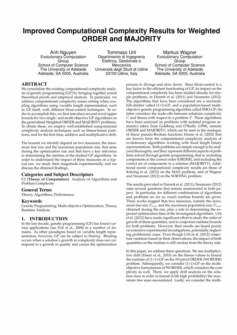
For a given solutionX , the fitness value is computed by pars-ing the represented tree inorder. For WORDER, the weightwi of a variable xi contributes to the fitness of X iff xi isvisited in the inorder parse before all the xi in the tree. ForWMAJORITY, the weight of xi contributes to the fitness ofXiff the number of occurrences of xi in the tree is at least oneand not less than the number of occurrence of xi (see Fig-ures 2 and 3). We call a variable redundant if it occurs multi-ple times in the tree; in this case the variable contributes onlyonce to the fitness value. The goal of WORDER and WMA-JORITY problems is to maximize their function values. Weillustrate both problems by an example (see Figure 1).

MO-WORDER and MO-MAJORITY are variants of the above-described problems, which take the complexityC of a syntaxtree (computed by the number of leaves of the tree) as thesecond objective:

• MO-WORDER (X) = (WORDER (X), C(X))• MO-WMAJORITY (X) = (WMAJORITY (X), C(X))

Figure 1: Example for evaluations according to WORDERand WMAJORITY. Let n = 5 and w1 = 15, w2 = 14,w3 = 12, w4 = 7, and w5 = 2. For the shown treeX , we get (after inorder parsing) l = (x1, x5, x4, x2, x2).For WORDER, we get S = (x1, x4) and WORDER(X) =w1 + w4 = 22. For WMAJORITY, we get S = (x1, x4, x2)and WMAJORITY(X) = w1 + w4 + w2 = 36.

Input: a syntax tree XInit: l an empty leaf list, S is an empty statement list.

1. Parse X inorder and insert each leaf at the rear of l as itis visited.

2. Generate S by parsing l front to rear and adding ("ex-pressing”) a leaf to S only if it or its complement arenot yet in S (i.e. have not yet been expressed).

3. WORDER (X) =∑xi∈S wi

Figure 2: Computation of WORDER (X)

Optimization algorithms can then use this to cope with thebloat problem: if two solutions have the same fitness value,then the solution of lower complexity can be preferred. Inthe special case, where wi = 1 holds for all 1 ≤ i ≤ n, wehave the problems:

• MO-ORDER (X) = (ORDER (X), C(X))

• MO-MAJORITY (X) = (MAJORITY (X), C(X))

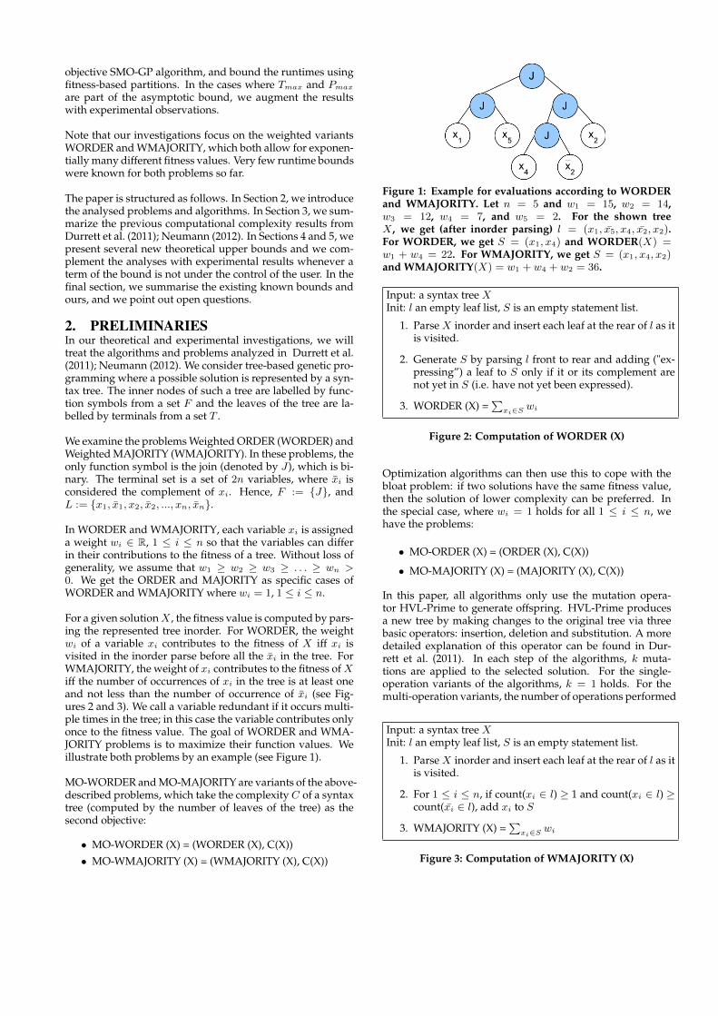
In this paper, all algorithms only use the mutation opera-tor HVL-Prime to generate offspring. HVL-Prime producesa new tree by making changes to the original tree via threebasic operators: insertion, deletion and substitution. A moredetailed explanation of this operator can be found in Dur-rett et al. (2011). In each step of the algorithms, k muta-tions are applied to the selected solution. For the single-operation variants of the algorithms, k = 1 holds. For themulti-operation variants, the number of operations performed

Input: a syntax tree XInit: l an empty leaf list, S is an empty statement list.

1. Parse X inorder and insert each leaf at the rear of l as itis visited.

2. For 1 ≤ i ≤ n, if count(xi ∈ l) ≥ 1 and count(xi ∈ l) ≥count(xi ∈ l), add xi to S

3. WMAJORITY (X) =∑xi∈S wi

Figure 3: Computation of WMAJORITY (X)

Mutate Y by applying HVL-Prime k times, In each time,randomly choose either insert, subsitute or delete.

• Insert: Choose a variable u ∈ L uniformly at randomand select a node v ∈ Y uniformly at random. Replacev by a join node whose children are u and v, in whichtheir orders are chosen randomly,

• Substitute: Replace a randomly chosen leaf v ∈ Y bya randomly chosen leaf u ∈ L.

• Delete: Choose a leaf node v ∈ Y randomly with par-ent p and sibling u. Replace p by u and delete p andu.

Figure 4: HVL-Prime mutation operator

is drawn each time from the distribution k = 1 + Pois(1),where Pois(1) is the Poisson distribution with parameter 1.

3. THEORETICAL RESULTSThe computational complexity analysis of genetic program-ming analyses the expected number of fitness evaluationsuntil the algorithm has produced an optimal solution for thefirst time. This is called the expected optimization time. Inthe case of multi-objective optimization the definition of ex-pected optimization time is slightly different and considersthe number of fitness evaluations until the whole Pareto front,i.e. the set of optimal trade-offs between the objectives, hasbeen computed.

The existing bounds from Durrett et al. (2011); Neumann (2012)are listed in Table 1. As it can be seen, all results for (1+1)-GPtake into account tree sizes of some kind: either the maxi-mum tree size Tmax found during search or the initial treeTinit size play a role in determining the bound. While Tinitis something which can be decided in advance, Tmax is a re-sult of the interactions between the fitness function, the set ofmutations and the selection process. As mutations involve adegree of randomness, in some cases such a measure is verydifficult to control.

A similar problem arises when dealing with multi-objectivealgorithms, such as SMO-GP. As we will see, the maximumpopulation size reached during optimization, Pmax, is a fun-damental term in most bounds and it is again very difficult totackle when a random number of mutations is involved. Thisis the paramount reason for which the only bounds for thesingle-mutation variant are known to date. Lastly, note thatthe upper bounds marked with ? hold only if the algorithmhas been initialized in the particular, i.e. non-redundant, waydescribed in Neumann (2012).

Because of the direct relation between these measures andthe bounds, investigating their magnitude is key to the fun-damental understanding of the bounds meaning.

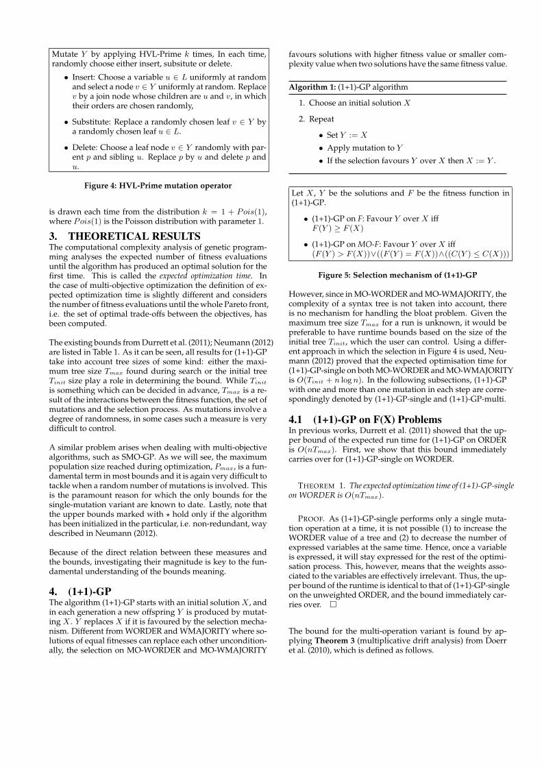
4. (1+1)-GPThe algorithm (1+1)-GP starts with an initial solution X , andin each generation a new offspring Y is produced by mutat-ing X . Y replaces X if it is favoured by the selection mecha-nism. Different from WORDER and WMAJORITY where so-lutions of equal fitnesses can replace each other uncondition-ally, the selection on MO-WORDER and MO-WMAJORITY

favours solutions with higher fitness value or smaller com-plexity value when two solutions have the same fitness value.

Algorithm 1: (1+1)-GP algorithm

1. Choose an initial solution X

2. Repeat

• Set Y := X

• Apply mutation to Y

• If the selection favours Y over X then X := Y .

Let X , Y be the solutions and F be the fitness function in(1+1)-GP.

• (1+1)-GP on F: Favour Y over X iffF (Y ) ≥ F (X)

• (1+1)-GP on MO-F: Favour Y over X iff(F (Y ) > F (X))∨((F (Y ) = F (X))∧((C(Y ) ≤ C(X)))

Figure 5: Selection mechanism of (1+1)-GP

However, since in MO-WORDER and MO-WMAJORITY, thecomplexity of a syntax tree is not taken into account, thereis no mechanism for handling the bloat problem. Given themaximum tree size Tmax for a run is unknown, it would bepreferable to have runtime bounds based on the size of theinitial tree Tinit, which the user can control. Using a differ-ent approach in which the selection in Figure 4 is used, Neu-mann (2012) proved that the expected optimisation time for(1+1)-GP-single on both MO-WORDER and MO-WMAJORITYis O(Tinit + n logn). In the following subsections, (1+1)-GPwith one and more than one mutation in each step are corre-spondingly denoted by (1+1)-GP-single and (1+1)-GP-multi.

4.1 (1+1)-GP on F(X) ProblemsIn previous works, Durrett et al. (2011) showed that the up-per bound of the expected run time for (1+1)-GP on ORDERis O(nTmax). First, we show that this bound immediatelycarries over for (1+1)-GP-single on WORDER.

THEOREM 1. The expected optimization time of (1+1)-GP-singleon WORDER is O(nTmax).

PROOF. As (1+1)-GP-single performs only a single muta-tion operation at a time, it is not possible (1) to increase theWORDER value of a tree and (2) to decrease the number ofexpressed variables at the same time. Hence, once a variableis expressed, it will stay expressed for the rest of the optimi-sation process. This, however, means that the weights asso-ciated to the variables are effectively irrelevant. Thus, the up-per bound of the runtime is identical to that of (1+1)-GP-singleon the unweighted ORDER, and the bound immediately car-ries over.

The bound for the multi-operation variant is found by ap-plying Theorem 3 (multiplicative drift analysis) from Doerret al. (2010), which is defined as follows.

F(X)(1+1)-GP, F(X) Durrett et al. (2011) (1+1)-GP, MO-F(X) Neumann (2012) SMO-GP, MO-F(X) Neumann (2012)

k=1 k=1+Pois(1) k=1 k=1+Pois(1) k=1 k=1+Pois(1)

ORDER O(nTmax) O(nTmax) O(Tinit + n logn)

?

O(nTinit + n2 logn)

WORDER ? ? O(Tinit + n logn) O(n3)? ?

MAJORITY O(n2Tmax logn) ? O(Tinit + n logn) O(nTinit + n2 logn)

WMAJORITY ? ? O(Tinit + n logn) O(n3)? ?

Table 1: Computational complexity results from Durrett et al. (2011); Neumann (2012)

THEOREM 2 (MULT. DRIFT, DOERR ET AL. (2010)). LetS ⊆ R be a finite set of positive numbers with minimum smin.Let X(t)

t∈N be a sequence of random variables over S ∪ 0. LetT be the random variable that denotes the first point in time t ∈ Nfor which X(t) = 0.

Suppose that there exists a constant δ > 0 such that

E[X(t) −X(t+1)|X(t) = s

]≥ δs (1)

holds for all s ∈ S with Pr[Xt = s] > 0. Then for all s0 ∈ S withPr[X(0) = s0] > 0,

E[T |X(0) = s0] ≤ 1 + log(s0/smin)

δ. (2)

In the following theorem we employ Theorem 2 to providean upper bound on the expected runtime of (1+1)-GP-multi,F(X) on WORDER when starting from any solution.

THEOREM 3. The expected optimization time of (1+1)-GP-multion WORDER is O(nTmax(logn+ logwmax)).

PROOF. In order to prove the stated bounds we need toinstantiate Theorem 2 on our problem. The theorem is validif we can identify a finite set S ⊆ R from which the randomvariables Xt are drawn. In our case the drift is defined onthe (at most exponentially many) values of the fitness func-tion. Also, since the result holds under the assumption thatthe underlying problem is a minimization problem, we firstneed to define an auxiliary problem WORDERmin which getminimized whenever WORDER gets maximized

WORDERmin(x) =

n∑i=1

wi −WORDER(x).

Note that while WORDER(x) is the sum of the weights forthe expressed variables in x, WORDERmin(x) is the sum ofthe weights of the unexpressed variables. We also recall thatORDER(x) denotes the number of expressed variables in x.

Now, given a solution xt at time t, let st = WORDERmin(xt)be the WORDER-value of this solution andm = n−ORDER(xt)the number of unexpressed variables in xt. Since an im-provement can be done by inserting a non-expressed vari-ables into the current tree, then the expected increment, i.e.

the drift, of WORDERmin is lower bounded by:

E[X(t) −X(t+1)|X(t) = st

]≥ WORDERmin(xt)

m· m

6enTmax

=WORDERmin(xt)

6enTmax

since the probability of expressing any of the m unexpressedvariables at the beginning of the tree is at least m

2n· 1

3eTmax=

m6enTmax

for both the single- and the multi-operation case,and the expected improvement when performing such stepis WORDERmin(xt)/m (because the missing weights aredistributed over m variables).

Given this drift, we have (in Theorem 2 terminology)

δ =1

6enTmax

s = WORDERmin(xt).

Also, from the definition of WORDER, we have that smin =wmin. From Theorem 2 follows that, for any initial value s0 =WORDERmin(x0), we have

E[T |X(0) = s0] ≤(

1 + ln

(s0

wmin

))· δ−1

≤(

1 + ln

(s0

wmin

))· 6enTmax.

Since we are interested in an upper bound over the expectedoptimization time, we must consider starting from the worstpossible initial solution, i.e. where none of the variables isexpressed. Let wmax be the largest weight in the set, then themaximum distance from the optimal solution is nwmax ≥ s0.Hence we have

E[T ] ≤(

1 + ln

(nwmaxwmin

))· 6enTmax

≤ (1 + ln (nwmax)) · 6enTmax= O(nTmax log(nwmax)) = O(nTmax(logn+ logwmax))

which states that the expected optimization time T of (1+1)-GP,F(X) for WORDERmin, and hence for WORDER, starting fromany solution is bounded byO(nTmax(logn+logwmax)).

The dependence of this bound, and of the bound for OR-DER introduced in Durrett et al. (2011), on Tmax is easily ex-plained by the fact that, in order to guarantee a single-stepimprovement, one must perform a beneficial insertion, i.e.one which expresses one of the unexpressed variables, at thebeginning of the tree. This involves selecting one out of at

most Tmax nodes in the tree. Unfortunately, Tmax can po-tentially grow arbitrarily large since F (X) does not controlsolution complexity.

We have investigated this measure experimentally in order tounderstand what its typical magnitude is. The experimentswere performed on AMD Opteron 250 CPUs (2.4GHz), onDebian GNU/Linux 5.0.8, with Java SE RE 1.6 and were givena maximum runtime of 3 hours and a budget of 109 evalua-tions. Furthermore, each experiment (involving two differ-ent initialization schemes, respectively with 0 and 2n leavesin the initial tree) has been repeated 400 times, which resultsin a standard error of the mean of 1/

√400 = 5%. The empir-

ical distributions of maximum tree sizes for (1+1)-GP, F (X)on all ORDER variants are shown as box-plots in Figure 6.The blue-toned line plots show the median Tmax divided byn (solid line) and by n log(n) (dashed line); the nearly con-stant behavior of the solid line suggests that Tmax has typi-cal a linear behavior, at least for the tested values of n andthe employed initialization schemes, for all the variants ofORDER.

4.2 Algorithms on MO-F(X) ProblemsFor the multi-operation variants, a single HVL-Prime appli-cation can lead to more than a single mutation with constantprobability. This would lead to the case where the complex-ity increase faster than the fitness value, i.e. an improvementon the fitness of the tree can be followed by multiple increaseon the complexity. We start our analysis by showing an up-per bound of the maximum tree size, Tmax, during run timeand then using that fact to bound the expected optimisationtime of (1+1)-GP-multi on MO-WORDER.

THEOREM 4. (Oliveto and Witt, 2011) Let Xt, t ≥ 0, be therandom variables describing a Markov process over a finite statespace S ⊆ R+

0 and denote ∆t(i) := (Xt+1 − Xt | Xt = i)for i ∈ S and t ≥ 0. Suppose there exists an interval [a, b] inthe state space, two constants δ, ε > 0 and, possibly depending onl := b− a, a function r(l) satisfying 1 ≤ r(l) = o(l/log(l)) suchthat for all t ≥ 0 the following two conditions hold:

1. E(∆t(i)) ≥ ε for a < i < b,

2. Prob(∆t(i) ≤ −j) ≤ r(l)

(1+δ)jfor i > a and j ∈ N0.

Then there is a constant c∗ > 0 such that for T ∗ := mint ≥ 0 :

Xt ≤ a | X0 ≥ b it holds Prob(T ∗ ≤ 2c

∗l/r(l))

= 2−Ω(l/r(l)).In the conference version, r(l) was only allowed to be a constant,i.e., r(l) = O(1). In this case, the last statement is simplified to

Prob(T ∗ ≤ 2c∗l) = 2−Ω(l).

THEOREM 5. Let Tinit ≤ 19n be the complexity of the initialsolution. Then, the maximum tree size encountered by(1+1)-GP-multi on MO-WORDER in less than exponential timeis 20n, with high probability.

Note that the state space S (of the tree sizes) is finite for bothproblems, as at most 2n fitness improvements are accepted.Thus, at most 2n + 1 different tree sizes can be attained.

PROOF. Theorem 4 was used to find the lower bound valueof a function in less than exponential time. In case of findingthe upper bound value of a function, condition 1 and 2 ofTheorem 4 are then changed to :

1. E(∆t(i)) ≤ −ε for a < i < b and ε > 0,

2. Prob(∆t(i) ≥ j) ≤ r(l)

(1+δ)jfor i > a and j ∈ N0.

Let a = 19n, b = 20n, k be the number of expressed vari-ables, and s be the number of leaves of the current tree. Forcondition 1 to hold, the expected drift of the size of a syn-tax tree in the interval [a, b] = [19n, 20n] must be a negativeconstant. This is computed by

E(∆t(i)) =∑j∈Z

j · P (∆t(i) = j)

=∑

j∈Z,j<0

j · P (∆t(i) = j) +∑j∈N

j · P (∆t(i) = j)

=∑j∈N

−j · P (∆t(i) = −j) +∑j∈N

j · P (∆t(i) = j)

When ∆t(i) = −j for j ∈ N, then the tree size is reduced byj. We can find a lower bound to the expected decrease in sizeby observing that to obtain a reduction of −j, we can do inprinciple t > j operations, out of which j must be deletionsof redundant variables and the other t − j must be neutralmoves. Since we have three mutations with equal probabil-ity of being selected, there are at least to 3t−j possible combi-nations of mutations that lead to a decrease of −j. We knowthat among these, at least one is made of substitutions thatdon’t decrease the fitness and the probability of obtaining it1/3t−j . Let s = cn, 19 < c < 20, then∑j∈N

−j · P (∆t(i) = −j)

≤ −∑j∈N

j

∞∑t=j

[(1

3

)j (s− kj

)(1

s

)j· 1

3t−s· Pois(x = t)

]

≤ −∑j∈N

j

∞∑t=j

[(1

3

)j (s− kj

)(1

s

)j· 1

3t−s· 1

et!

]

≤ − 1e

∑j∈N

j

(1

3

)j·(s− kj

)j·(

1

s

)j ∞∑t=j

(1

3t−s· 1

t!

)≤ − 1

e

∑j∈N

j

(1

3

)j·(c− 1

c

)j·(

1

j

)j ∞∑t=j

(1

3t−s· 1

t!

)where (1/3)j comes from the fact that we need to perform jdeletions, (1/s)j is related to selecting the right leaf over sleaves for j times and

(s−kj

)is the number of possible per-

mutations of redundant variables.

When ∆t(i) = j for j ∈ N, the size of the tree increases. Inorder to provide a upper bound on the expected increase ofthe tree size, we need to consider all the possible combina-tions of t mutations which lead us to an increase of j. Sincewe need to increase the tree size by j, we need at least j in-sertions, thus the remaining t− j mutations can be arrangedin 3t−j different ways. Note that this is an upper bound, asmany of these combinations will not lead to an increase ofj. This means that the probability to do a correct number of

Figure 6: Distribution, as green box-plots, of the maximum tree sizes observed for (1+1)-GP, F (X) on the ORDER variants.The blue-toned lines are the median Tmax values divided by the corresponding polynomial (see the legend) and suggest theasymptotic behavior of the measure. In this case the almost horizontal line for n shows that the maximum tree size is veryclose to linear, at least for the tested input sizes.

insertions is upper bounded by

3t−j

3t=

1

3j

Also, in order to accept a larger tree size, the fitness must beincreased as well. In the worst case, this can be accomplishedby inserting one unexpressed variable in such a position thatit increases the fitness of the tree size, an inserting m − 1random variables in positions that don’t decrease the fitnessof the tree. Thus the expected increase in the tree size is∑

j∈N

j · P (∆t(i) = j)

≤∑j∈N

(j · n− k

2n· P1 · P2

∑t=j

Pois(x = t)

)

≤∑j∈N

(j · 1

3j· 1

2

∑t=j

1

et!

)

=1

e

∑j∈N

(j · 1

2· 1

3j

∑t=j

1

t!

)

where the (1/3)j term comes from the fact that we want todo j insertions, (n− k)/2n comes from the fact that we want

to insert one of the unexpressed variables, P1 comes fromthe fact that we want to insert the unexpressed variable ina position where it can determine an increase in the fitness,and P

(j−1)2 comes from the fact that we want to put j − 1

(possibly redundant) random variables (whose probability 1of being selected has been omitted) at any position in whichthey don’t determine a decrease in the fitness. Also note thatP1, P2 ≤ 1 and n− k/2n ≤ 1/2. Therefore, we have that

E(∆t(i)) =∑j∈N

−j · P (∆t(i) = −j) +∑j∈N

j · P (∆t(i) = j)

≤ −1

e

∑j∈N

[j

j!·(

1

3

)j·(

1

cn

)j·(

(c− 1)n

j

)j·

∞∑t=j

(1

3t−s· 1

t!

)]+∑j∈N

(j · 1

2· 1

3j· 1

e

∑t=j

1

t!

)

=1

e

∑j∈N

(j

3j·

[1

2

(∑t=j

1

t!

)− 1

j!·(c− 1

c

)j·

1

jj

(1

j!

1

3 · (j + 1)!

)])

Let A =∑j∈NAj , where

Aj = j3j ·

[12

∑t=j

1t!−(c−1c

)j 1jj

∑t=j

(1

3t−j1t!

)]in which

∑t=j

(1

3t−j1t!

)≥(

1j!

13·(j+1)!

)for 19 < c < 20, we have

A1 <1

3·(e− 1

2− 19

20(1 + 1/6)

)= −0.083064

A2 <2

9·

(e− 2

2−(

19

20

)2

· 1

4(1/2 + 1/18)

)= 0.051954

A3 <1

9·

(e− 2− 0.5

2−(

19

20

)3

· 1

27(1/6 + 1/72)

)= 0.011490

Hereby,

A = A1 +A2 +A3 +∑j≥4

Aj < −0.019620 +∑j≥4

Aj

However, since

∑j≥4

Aj =∑j≥4

j

3j·

[1

2

∑t=j

1

t!−(c− 1

c

)j1

jj

∑t=j

(1

3t−j1

t!

)]

<∑j≥4

j

3j·

(1

2

∑t=j

1

t!

)

<∑j≥4

j

3j· e− 2− 0.5− 1/6

2

< 0.025808 ·∑j≥4

j

3j

≤ 0.025808 · 1/3

(1− 1/3)2= 0.019356

This gives us

A = A1 +A2 +A3 +∑j≥4

Aj

= −0.000264

Therefore E(∆t(i)) = 1e·A < 0, and condition 1 holds.

For condition 2 to hold, in order to increase the number ofnodes of the original tree by j, at least j insertions must bemade. Thus, the probability that the tree size increases ex-actly by j is at most

P (∆i = j) ≤ 1

e·

(1

2· 1

3j

∑t=j

1

t!

)

≤ 1

e· 1

3j· 1

2·∑t=j

1

t!

≤ 1

3j

Hence,

P (∆i ≥ j) =

∞∑k=j

P (∆i = k)

≤∞∑k=j

1

3j=

∞∑k=1

1

3j−j−1∑k=1

1

3j

=

∞∑k=0

1

3j− 1−

[j−1∑k=0

1

3j− 1

]

=1

1− 1/3− 1− (1/3)j

1− 1/3=

3

2

1

3j

Let r(l) be a constant and δ = 2, then condition 2 holds.

THEOREM 6. Starting with an solution with initial size Tinit <19n , the optimization time of (1+1)-GP-multi on MO-ORDER isO(n2 logn), with high probability.

PROOF. This algorithm contains multiple phases. At eachphase, there are two main tasks:

• Delete all the redundant variables in the current tree toobtain a non-redundant tree.

• Insert an unexpressed variable into the tree to improvethe fitness

The algorithm terminates when all of n variables are expres-sed and the tree size is n. Let ki, ji be the number of theredundant and expressed variables of the solution at the be-ginning of phase i. The expected time Ti to delete all of theredundant variables at phase i is upper bounded by

Ti =

ki∑l=1

(1

3e)−1 · ( l

l + ji)−1 ≤ 3e

ki∑l=1

l + n

l

≤ 3e

n∑l=1

l + n

l+ 3e

ki∑l=n+1

l + n

l

≤ 3e

n∑l=1

l + n

l+ 3e

ki∑l=n+1

2

≤ O(n logn) + 2ki

An unexpressed variable is then chosen and inserted in tothe tree in any position to improve the fitness. The expectedtime to do such a step is n−ji

6en. Therefore, the expected time

for a single phase is O(n logn) + 2ki + n−ji6en

.

The selection mechanism of (1+1)-GP on MO-F(X) problemsdoes not accept any decrease in the fitness of the solution.Thus, ji increases during the run time, which we can denoteas j0 = 0 < j1 = 1 < ... < jn−1 = n − 1. Since there are atmost n variables that need to be inserted, there are at most nphases need to be done to obtain the optimal tree. The total

runtime is then, with high probability, bounded by:

n−1∑j=0

O(n logn) + 2ki +

(n− j6en

)−1

≤ O(n2 logn) + 2

n−1∑j=0

E [Tmax] + 6en

n−1∑j=0

i

n− j

≤ O(n2 logn) + 40n2 + 6enO(logn)

≤ O(n2 logn)

After n phases, the current tree now has the highest fitnessvalue. The last step now is to remove all of the redundantvariables to obtain a tree with highest fitness and complexityvalue of n. Let s be the number of leaves, the expected timefor this step is upper bounded by:

4n∑s=n+1

(1

3e· s− n

s

)−1

= 3e

3n∑j=1

j + n

j

= 3e

n∑j=1

j + n

j+ 3e

2n∑j=n+1

j + n

j+ 3e

3n∑j=2n+1

j + n

j

≤ 3e ·n∑j=1

j + n

j+ 3e ·

2n∑j=n+1

2 + 3e

3n∑j=2n+1

3

2

= O(n logn) +O(n)

Summing up the runtimes for all the tasks, the optimizationtime of (1+1)-GP-multi on MO-ORDER is O(n2 logn) withhigh probability.

5. MULTI-OBJECTIVE ALGORITHMSIn SMO-GP, the complexity C(X) of a solution X is alsotaken into account and treated as equally important as thefitness value F (X). The classical Pareto dominance relationsare:

1. A solutionX weakly dominates a solution Y (denoted byX Y ) iff (F (X) ≥ F (Y ) ∧ C(X) ≤ C(Y )).

2. A solution X dominates a solution Y (denoted by X Y ) iff ((X Y ) ∧ (F (X) > F (Y ) ∨ C(X) < C(Y )).

3. Two solutions X and Y are called incomparable iff nei-ther X Y nor Y X holds.

A Pareto optimal solution is a solution that is not dominatedby any other solution in the search space. All Pareto opti-mal solutions together form the Pareto optimal set, and theset of corresponding objective vectors forms the Pareto front.The classical goal in multi-objective optimization (here: ofSMO-GP) is to compute for each objective vector of the Paretofront a Pareto optimal solution. Alternatively, if the Paretofront is too large, the goal then is to find a representativesubset of the front, where the definition of ‘representative’depends on the choice of the conductor.

SMO-GP starts with a single solution, and at all times keepsa population that contains only the non-dominated solutionsamong the set of solutions seen so far.

Algorithm 2: SMO-GP

1. Choose an initial solution X

2. Set P := X

3. repeat

• Randomly choose X ∈ P• Set Y := X

• Apply mutation to Y

• If Z ∈ P |Z Y = ∅ setP := (P\Z ∈ P |Y Z) ∪ Y

In his paper, Neumann (2012) proved that the expected opti-mization time of SMO-GP-single and SMO-GP-multi on MO-ORDER and MO-MAJORITY is O(nTinit + n2 logn). In thecase of WORDER and WMAJORITY, the proven runtimebound of O(n3) (for both problems) requires that the algo-rithm is initialised with a non-redundant solution.

5.1 SMO-GP-singleIf the initial solution is generated randomly, it is not likely tobe a non-redundant one. In order to generalise the proof, westart the analysis by bounding the maximum tree size Tmaxbased on the initial tree size Tinit for SMO-GP-single. Usingthis result, we re-calculate the expected optimization time ofSMO-GP-single on both MO-WORDER and MO-WMAJORITY,when using an arbitrary initial solution of size Tinit.

THEOREM 7. Let Tinit be the tree size of initial solution. Thenthe population size of SMO-GP-single on MO-WORDER and MO-WMAJORITY until the empty tree included in the population isupper bounded by T init + n during the run of the algorithm.

PROOF. When two solutions X , Y have the same com-plexity, the solution with higher fitness dominates the otherone. Therefore, in the population where no solution is domi-nated by any other solutions, all the solutions have differentcomplexities. Without loss of generality, assume that a so-lution X is selected for mutation and Y is the new solution.Then there are five ways to generate Y :

1. inserting an unexpressed variable, and thus increasingthe complexity of the new solution by 1,

2. deleting an expressed variable, and thus decreasing thecomplexity of the new solution by 1,

3. deleting a redundant variable, and thus decreasing thecomplexity of the new solution by 1. AsF (X) = F (Y )∧C(X) > C(Y ), X is then replaced by Y in the popula-tion,

4. inserting a redundant variable to X , thus generatinga new solution with the same fitness and higher com-plexity, which is not accepted by SMO-GP-single,

5. substituting a variable xi in X by another variable xj .

• If xj is a non-redundant variable and wi < wj ,F (X) < F (Y ) ∧ C(X) = C(Y ), Y replaces X inthe population

• If xj is a non-redundant variable and wi > wj ,F (X) > F (Y ) ∧ C(X) = C(Y ), Y is discarded.

• If xj is redundant variable, F (X) > F (Y )∧C(X) =C(Y ), Y is discarded.

As shown above, the number of redundant variables in thesolution will not increase during the run of the algorithm.Let Ri be the number of redundant variables in solution i,then for all the solutions in the population holds Ri ≤ Rinit.

Let X ∈ P be a solution in P and αX be the number of ex-pressed variables in X , then the complexity of X is C(X) =RX + αX . Since RX ≤ Rinit and αX ≤ n, the complexity ofa solution in P is upper bounded by Rinit + n ≤ Tinit + n.

The population size only increases when a new solution withdifferent fitness is generated. This only happens when thecomplexity increases or decreases by 1. Because the highestcomplexity that a solution can reach is Tinit+n, and becausethe empty tree can be in the population as well1, the maxi-mum size the population can reach is Tinit + n+ 1.

LEMMA 1. Starting with an arbitrary initial solution of sizeTinit , the expected time until the population of SMO-GP-single onMO-WORDER and MO-WMAJORITY contains the empty tree isO(T 2

init + nTinit).

PROOF. We will bound the time by repeated deletions ofrandomly chosen leaf nodes in the solutions of lowest com-plexity, until the empty tree has been reached. Let X be thesolution in the population with the lowest complexity. Theprobability of choosing the lowest complexity solution X inthe population is at least 1

Tinit+n+1, while the probability of

making a deletion is 13

. In each step, because any variable inX can be deleted, the probability of choosing the correct vari-able is 1. The probability of deleting a variable in X at eachstep therefore is bounded from below by 1

3· 1Tinit+n+1

, andthe expected time to do such a step is at most 3·(Tinit+n+1).Since Tinit is the number of leaves in the initial tree, there areTinit repetitions required to delete all the variables. This im-plies that the expected time for the empty tree to be includedin the population is upper bounded by

Tinit · 3 · (Tinit + n+ 1) = O(T 2init + nTinit

)THEOREM 8. Starting with a single arbitrary initial solution

of size Tinit, the expected optimization time of SMO-GP-single onMO-WORDER and MO-WMAJORITY is O(T 2

init + n2Tinit +n3).

PROOF. In the following steps, we will bound the timeneeded to discover the whole Pareto front, once the emptysolution is introduced into the population. As shown in The-orem 1, the empty tree is included in the population after1as the empty tree is Pareto optimal with F (X) = C(X) = 0

O(T 2init + nTinit) steps. The empty tree is now a Pareto op-

timal solution with complexity C(X) = 0. Note that a so-lution of complexity j, 0 ≤ j ≤ n is Pareto optimal in MO-WORDER and MO-MAJORITY, if it contains only the largestj variables.

Let us assume that the population contains all Pareto optimalsolutions with complexities j, 0 ≤ j ≤ i. Then, a populationwhich includes all Pareto optimal solutions with complexi-ties j, 0 ≤ j ≤ i+ 1, can be achieved by producing a solutionY that is Pareto optimal and that has complexity i+ 1. Y canbe obtained from a Pareto optimal solutionX with C(X) = i

and F (X) =∑ki=1 wi by inserting the leaf xk+1 (with associ-

ated weight wk+1) at any position. This operation producesfrom a solution of complexity i a solution of complexity i+1.

Based on this idea we can bound the expected optimizationtime once we can bound the probability for such steps to hap-pen. Choosing X for mutation has the known probabilityof at least 1

Tinit+n+1as the population size is upper bound

by Tinit + n + 1. Next, the inserting operation of the muta-tion operator is chosen with probability 1

3. As a specific ele-

ment out of a total of n elements has to be inserted at a ran-domly chosen position, the probability to do so it 1

n. Thus,

the total probability of such a generation is lower boundedby 1

Tinit+n+1· 1

3· 1n

.

Now, we use the method of fitness-based partitions Wegener(2002) according to the n + 1 different Pareto front sizes i.Thus, as there are only n Pareto-optimal improvements pos-sible once the empty solution is introduced into the popula-tion, the expected time until all Pareto optimal solutions havebeen generated is:

n−1∑i=0

(1

Tinit + n+ 1· 1

3· 1

n

)−1

= 3n2(Tinit + n+ 1)

= O(n2Tinit + n3).

Summing up the number of steps to generate the empty treeand all other Pareto optimal solutions, the expected optimi-sation time is O(T 2

init + n2Tinit + n3)

5.2 SMO-GP-multiIn principle, when considering WORDER and WMAJORITYin SMO-GP, it is possible to generate an exponential numberof trade-offs between solution fitness and complexity. For in-stance, if wi = 2n−i, 1 ≤ i ≤ n, then one can easily generate2n different individuals by considering different subsets ofvariables. These solutions are dominated by the true Paretofront, and our experimental analysis suggests that many ofthem get discarded early in the optimization process.

In this section, we employ the Pmax measure collected in ourexperimental analysis (see Figure 7) to consolidate some ofthe theoretical bounds about WORDER and WMAJORITYpresented in Neumann (2012) and introduce new bounds fortheir multi-operation variants.

LEMMA 2. The expected time before SMO-GP, initialized withTinit leaves, adds the empty tree to its population is bound byO(TinitPmax).

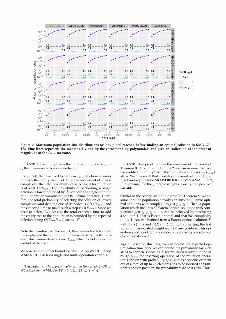
Figure 7: Maximum population size distributions (as box-plots) reached before finding an optimal solution in SMO-GP.The blue lines represent the medians divided by the corresponding polynomials and give an indication of the order ofmagnitude of the Pmax measure.

PROOF. If the empty tree is the initial solution, i.e. Tinit =0, then Lemma 2 follows immediately.

If Tinit > 0, then we need to perform Tinit deletions in orderto reach the empty tree. Let X be the individual of lowestcomplexity, then the probability of selecting it for mutationis at least 1/Pmax. The probability of performing a singledeletion is lower bounded by 1

3efor both the single- and the

multi-operation variants of the HVL-Prime operator. There-fore, the total probability of selecting the solution of lowestcomplexity and deleting one of its nodes is Ω(1/Pmax), andthe expected time to make such a step is O(Pmax). Since weneed to delete Tinit leaves, the total expected time to addthe empty tree to the population is bounded by the repeateddeletion taking O(TinitPmax) steps.

Note that, contrary to Theorem 1, this lemma holds for boththe single- and the multi-mutation variants of SMO-GP. How-ever, this lemma depends on Pmax, which is not under thecontrol of the user.

We now state an upper bound for SMO-GP on WORDER andWMAJORITY in both single and multi-operation variants.

THEOREM 9. The expected optimization time of SMO-GP onWORDER and WMAJORITY is O(Pmax(Tinit + n2)).

PROOF. This proof follows the structure of the proof ofTheorem 8. First, due to Lemma 2 we can assume that wehave added the empty tree to the population afterO(TinitPmax)steps. We now recall that a solution of complexity j, 0 ≤ j ≤n, is Pareto optimal for MO-WORDER and MO-WMAJORITY,if it contains, for the j largest weights, exactly one positivevariable.

Similar to the second step of the proof of Theorem 8, we as-sume that the population already contains the i Pareto opti-mal solutions with complexities j, 0 ≤ j ≤ i. Then, a popu-lation which includes all Pareto optimal solutions with com-plexities j, 0 ≤ j ≤ i + 1, can be achieved by producinga solution Y that is Pareto optimal and that has complexityi + 1. Y can be obtained from a Pareto optimal solution X

with C(X) = i and F (X) =∑ki=1 wi by inserting the leaf

xk+1 (with associated weight wk+1) at any position. This op-eration produces from a solution of complexity i a solutionof complexity i+ 1.

Again, based on this idea, we can bound the expected op-timization time once we can bound the probability for suchsteps to happen. Choosing X for mutation is lower boundedby 1/Pmax, the inserting operation of the mutation opera-tor is chosen with probability 1/3e, and as a specific elementout of a total of up to 2n elements has to be inserted at a ran-domly chosen position, the probability to do so it 1/2n. Thus,

the total probability of such a generation is lower boundedby 1/ (6enPmax).

Now, using the method of fitness-based partitions accordingto the n + 1 different Pareto front sizes i, the expected timeuntil all Pareto optimal solutions have been generated (oncethe empty tree was introduced) is bounded by

n−1∑i=0

(1

Pmax· 1

3e· 1

2n

)−1

= 6en2Pmax

= O(n2Pmax).

Therefore, the total expected optimization time when start-ing from an individual with Tinit leaves is thusO(TinitPmax+n2Pmax), which concludes the proof.

As we mentioned before, to date there is no theoretical un-derstanding about how Pmax grows during an optimizationrun and, in principle, its order of growth could be exponen-tial in n. For this reason, similarly to what we did for Tmax,we have investigated this measure experimentally. The ex-perimental setup is the same described previously, and theempirical distributions of Pmax are shown as box-plots inFigure 7. The blue-toned line plots show the median Pmaxdivided by n and log(n). Again, the nearly constant behav-ior of the solid line suggests a magnitude of Pmax which islinearly dependent on n and, in general, very close to n asthe factors, at most 1.1, suggest.

6. CONCLUSIONSIn this paper, we carried out theoretical investigations to com-plement the recent results on the runtime of two genetic pro-gramming algorithms (Durrett et al., 2011; Neumann, 2012;Urli et al., 2012). Crucial measures in the theoretical analysesare the maximum tree size Tmax that is attained during therun of the algorithms, as well as the maximum populationsize Pmax when dealing with multi-objective models.

We introduced several new bounds for different GP variantson the different versions of the problems WORDER and WMA-JORITY. Tables 2 and 3 summarise our results and the exist-ing known bounds on the investigated problems.

Despite the significant theoretical and experimental effort,the following open challenges still remain:

1. Almost no theoretical results for the multi-operationvariants are known to date. A major reason for this isthat it is not clear how to bound the number of acceptedoperations when employing the multi-operation vari-ants on the weighted cases.

2. Of particular difficulty seems to be the problem to boundruntimes on WMAJORITY. There, in order to achievea fitness increment, the incrementing operation needsto be preceded by a number of operations that reducethe difference in positive and negative occurrences of avariable. Said difference is currently difficult to control,as it can increase and decrease during a run.

3. Several bounds rely on Tmax or Pmax measures, whichare not set in advance and whose probability to increaseor decrease during the optimization is hard to predict.This is because their growth (or decrease) depends onthe content of the individual and the content of the pop-ulation at a specific time step. Solving these problemswould allow bounds which only depend on parame-ters the user can initially set. Observe that limitingTmax and Pmax is not an option, since we are consider-ing variable length representation algorithms, and pop-ulations that represent all the trade-offs between objec-tives.

4. Finally, it is not known to date how tight these boundsare.

ReferencesDoerr, B., Johannsen, D., and Winzen, C. (2010). Multiplica-

tive drift analysis. In Pelikan, M. and Branke, J., editors,GECCO, pages 1449–1456. ACM.

Droste, S., Jansen, T., and Wegener, I. (2002). On the analysisof the (1+1) evolutionary algorithm. Theoretical ComputerScience, 276:51–81.

Durrett, G., Neumann, F., and O’Reilly, U.-M. (2011). Com-putational complexity analysis of simple genetic program-ing on two problems modeling isolated program seman-tics. In FOGA, pages 69–80. ACM.

Goldberg, D. E. and O’Reilly, U.-M. (1998). Where does thegood stuff go, and why? How contextual semantics influ-ences program structure in simple genetic programming.In EuroGP, volume 1391 of LNCS, pages 16–36. Springer.

Kötzing, T., Sutton, A. M., Neumann, F., and O’Reilly, U.-M. (2012). The max problem revisited: the importanceof mutation in genetic programming. In Proceedings of thefourteenth international conference on Genetic and evolutionarycomputation conference, GECCO ’12, pages 1333–1340, NewYork, NY, USA. ACM.

Neumann, F. (2012). Computational complexity analysis ofmulti-objective genetic programming. In Proceedings of thefourteenth international conference on Genetic and evolutionarycomputation conference, GECCO ’12, pages 799–806, NewYork, NY, USA. ACM.

Oliveto, P. S. and Witt, C. (2011). Simplified drift analysis forproving lower bounds in evolutionary computation. Algo-rithmica, 59(3):369–386.

Poli, R., Langdon, W. B., and McPhee, N. F. (2008). A FieldGuide to Genetic Programming. lulu.com.

Urli, T., Wagner, M., and Neumann, F. (2012). Experimen-tal supplements to the computational complexity analysisof genetic programming for problems modelling isolatedprogram semantics. In PPSN. Springer. (to be published).

Wagner, M. and Neumann, F. (2012). Parsimony pressureversus multi-objective optimization for variable lengthrepresentations. In PPSN. Springer. (to be published).

Wegener, I. (2002). Methods for the analysis of evolutionaryalgorithms on pseudo-Boolean functions. In EvolutionaryOptimization, pages 349–369. Kluwer.

F(X)(1+1)-GP, F(X)

k=1 k=1+Pois(1)

ORDERO(nTmax) Durrett et al. (2011) O(nTmax) Durrett et al. (2011)

O(Tinit + n logn) Urli et al. (2012) O(Tinit + n logn) Urli et al. (2012)

WORDERO(nTmax) ? O(nTmax(logn+ logwmax)) ?

O(Tinit + n logn) Urli et al. (2012) O(Tinit + n logn) Urli et al. (2012)

MAJORITYO(n2Tmax logn) Durrett et al. (2011) ?O(Tinit + n logn) Urli et al. (2012) O(Tinit + n logn) Urli et al. (2012)

WMAJORITY? ?

O(Tinit + n logn) Urli et al. (2012) O(Tinit + n logn) Urli et al. (2012)

F(X)(1+1)-GP, MO-F(X)

k=1 k=1+Pois(1)

ORDERO(Tinit + n logn)Neumann (2012) O(n2 logn) ? †O(Tinit + n logn) Urli et al. (2012) O(Tinit + n logn) Urli et al. (2012)

WORDERO(Tinit + n logn)Neumann (2012) ?O(Tinit + n logn) Urli et al. (2012) O(Tinit + n logn) Urli et al. (2012)

MAJORITYO(Tinit + n logn)Neumann (2012) ?O(Tinit + n logn) Urli et al. (2012) O(Tinit + n logn) Urli et al. (2012)

WMAJORITYO(Tinit + n logn)Neumann (2012) ?O(Tinit + n logn) Urli et al. (2012) O(Tinit + n logn) Urli et al. (2012)

Table 2: Summary of our bounds (?) and the existing theoretical upper bounds from Table 1. The average-case conjecturesfrom Urli et al. (2012) are listed to indicate tightness. Note that (?) mark the cases for which no theoretical bounds are known,and bounds marked with (†) require special initialisations.

F(X)SMO-GP, MO-F(X)

k=1 k=1+Pois(1)

ORDERO(nTinit + n2 logn)Neumann (2012) O(nTinit + n2 logn)Neumann (2012)O(nTinit + n2 logn) Urli et al. (2012) O(nTinit + n2 logn) Urli et al. (2012)

WORDERO(T 2

init + n2Tinit + n3) ? O(TinitPmax + n2Pmax) ?

O(n3) Neumann (2012) †O(nTinit + n2 logn) Urli et al. (2012) O(nTinit + n2 logn) Urli et al. (2012)

MAJORITYO(nTinit + n2 logn)Neumann (2012) O(nTinit + n2 logn)Neumann (2012)O(nTinit + n2 logn) Urli et al. (2012) O(nTinit + n2 logn) Urli et al. (2012)

WMAJORITYO(T 2

init + n2Tinit + n3) ? O(TinitPmax + n2Pmax) ?

O(n3) Neumann (2012) †O(nTinit + n2 logn) Urli et al. (2012) O(nTinit + n2 logn) Urli et al. (2012)

Table 3: Summary of our bounds (?) and the existing theoretical upper bounds from Table 1. The average-case conjecturesfrom Urli et al. (2012) are listed to indicate tightness. Note that the bounds marked with (†) require special initialisations.