NASA-CR-192816

IMPROVED ASSUMED-STRESS HYBRID SHELL ELEMENT WITH

DRILLING DEGREES OF FREEDOM FOR LINEAR STRESS,

BUCKLING, AND FREE VIBRATION ANALYSES

Govind Rengarajan*

Glemson University, Glemson, SC 29634-092I

Mohammad A. Aminpour i"

Analytical Services and Materials, Inc., Hampton, VA 23666

Norman F. Knight, Jr. _t

Old Dominion University, Norfolk, VA 23529-0247

Abstract

An improved 4-node quadrilateral assumed-stress hybrid shell element with drilling

degrees of freedom is presented. The formulation is based on Hellinger-Reissner varia-

tional principle and the shape functions are formulated directly for the 4-node element.

The element has 12 membrane degrees of freedom and 12 bending degrees of freedom.

It has 9 independent stress parameters to describe the membrane stress resultant field

and 13 independent stress parameters to describe the moment and transverse shear

stress resultant field. The formulation encompasses linear stress, linear buckling, and

linear free vibration problems. The element is validated with standard test cases and

is shown to be robust. Numerical results are presented for linear stress, buckling, and

free vibration analyses.

* Graduate Research Assistant, Department of Mechanical Engineering, Currently at

Department of Mechanical Engineering, Texas A & M University, College Station,

TX 77843-3123.

t SeniorScie_ist.

AssociatePro_ssor, DepartmentofAerospaceEngineerin_.

(NASA-CR-192816) IMPROVED

ASSUMED-STRESS HYBRID SHELL ELEMENT

WITH DRILLING DEGREES OF FREEDOM

FOR LINEAR STRESS, BUCKLING, AND

FREE VIBRATION ANALYSES (C1emson

Univ.) 51 p

N95-13163

Unclas

G3/39 0027B13

https://ntrs.nasa.gov/search.jsp?R=19950006750 2018-06-10T16:38:41+00:00Z

Introduction

Today, the literature abounds with new shell element formulations and the key is-

sue is the robustness of individual elements. Factors that influence the robustness

of elements are spurious zero-energy modes, locking, convergence characteristics, ele-

ment invariance, and sensitivity to mesh distortion. Considerable progress has been

made over the years in addressing some of these factors and in developing suitable

assessment procedures and test cases to evaluate and vahdate the new elements. In

the process, several new techniques and new element formulations such as assumed-

stress, reduced-integration, incompatible modes, and assumed-strain have evolved,

that successfully address some of the problems associated with shell elements.

On a geometrical aspect, the shell element formulations that are currently avail-

able in literature can be broadly classified into three categories: curved elements based

on classical shell theories, degenerated solid shell elements, and flat shell elements.

The faceted representation of the shell geometry using flat shell elements is perhaps

the simplest of these approaches. These elements combine the membrane and bend-

ing behavior of plate elements. While the approximate geometrical representation is

immediately evident, particularly in 4-node bihnear elements, the simphcity of the

formulation, the convergence characteristics, and full rank has made this approach

very attractive. The inclusion of transverse shear effects with the aid of Reissner-

Mindhn kinematics, and more recently, the inclusion of drilling degrees of freedom

[1, 2], have significantly improved the performance of flat shell elements.

The assumed-stress hybrid formulations pioneered by Pian and his coworkers

[3] is variationally consistent and has led to the development of several powerful

element formulations. In general, the mixed/hybrid formulations are computationally

more intensive than the displacement-based formulations; however, using symbohc

manipulation (e.g., see [4]), and exploiting the banded structure of matrices, the

computational cost could be reduced significantly.

The objective of this paper is to present the formulation of an improved 4-node

assumed-stress hybrid shell element with drilling degrees of freedom. The formula-

tion encompasses hnear stress, hnear buckhng, and hnear free vibration problems.

The element is validated using standard test cases as well as a few other interesting

problems for hnear stress, buckling, and free vibration analyses. Wherever possible,

relevant matrices are generated symbohcally, and this has helped save considerable

computational time. However, the details of the symbolic manipulation will be dealt

with in a subsequent paper.

Drilling Degrees of Freedom

Drilling degrees of freedom are defined as the rotational degrees of freedom normal

to the plane of the element. The drilling rotation (_) is not represented in the mem-

brane kinematics of the shell. Consequently, the drilling degree of freedom is not

included at the element level; however at the global or assembled level, the degrees

of freedom associated with the structure may include the drilling degrees of freedom.

While assembhng the element stiffness matrices to form the global stiffness matrix, if

the elements connected to a particular node happen to be coplanar, then the drilling

rotation at that node is not resisted. This leads to a singularity in the stiffness matrix

[5]. This singularity could clearly be avoided if the drilling degree of freedom is in-

cluded in the variational statement or in the finite element approximations as will be

discussed subsequently. Yet another motivation to include the drilling degree of free-

dom stems from difficulties in modehng stiffened panels, folded plate structures, etc.

The lack of drilling rotation in such instances results in an inadequate representation

of the structural response.

Generally, the drilling degrees of freedom are suppressed at the beginning of the

analysis since they do not enter the kinematic description of the problem. Zienkiewicz

[6] associates a fictitious couple M_ with the rotation at the element level to resolve

2

the singularity problem. While this does take care of the singularity in the stiff-

ness matrix, it does not utilize the drilling degrees of freedom to improve the finite

element approximations. However, there have been numerous attempts in formulat-

ing elements with drilling degrees of freedom, and two significant approaches have

emerged successful. One approach is to introduce the drilling rotation in the varia-

tional statement as an independent variable, while the other approach is to introduce

the drilling rotation in the approximations of in-plane displacements.

Drilling Rotation in the Variational Statement

Reissner [7] presented a mixed variational principle in which the definition of true

rotations as the skew-symmetric part of the displacement gradients are relaxed and

later enforced in the variational statement as constraints through the introduction of

Lagrange multipliers. On imposing the stationary conditions on the functional, the

Lagrange multipliers are identified as the skew-symmetric part of the stress tensor.

This formulation introduced a rotation field independent of displacements. Hughes

and Brezzi [8] modified Reissner's functional by including an additional term that

stabihzes the functional in discrete approximations. Ibrahimbegovic et al. [9, 10]

used the modified formulation of Hughes and Brezzi and developed quadrilateral

membrane and flat shell elements. They used independent interpolation fields for

rotations and AUman-type [1] shape functions for the in-plane displacements. Iura

and Atluri [11] have developed an element where the rotations are interpolated from

true nodal rotations evaluated from the skew-symmetric part of the displacement

gradient at the nodes.

Drilling Rotations in Finite Element Approximations

In early attempts, the drilling rotation was introduced in the shape functions

using a cubic displacement function (e.g., see Robinson [12]). However, Irons and

3

Ahmad [13] pointed out that this method had some difficulties and convergence was

not assured. The elements formed in such a manner force the shearing strain to be

zero at the nodes and do not pass the patch test. Recently, the drilling rotations have

been introduced in the finite element approximations successfully using quadratic dis-

placement functions [1,2,14-18]. In this approach, the membrane element is internally

assumed to be an 8-node element (four corner nodes and four midside nodes) with 16

degrees of freedom. The stiffness matrix of this 8-node element is then condensed to

that of a 4-node element (four corner nodes) with 12 degrees of freedom by associat-

ing the displacement degrees of freedom at the midside nodes with the displacement

and rotational degrees of freedom at the corner nodes. In effect, the in-plane dis-

placements are dependent on in-plane rotations. MacNeal and Harder [16] have used

the above approach to develop a 4-node membrane element with selectively reduced

integration. Yunus et al. [17] have also used this approach to develop assumed-stress

hybrid elements. Aminpour [18, 19] has developed assumed-stress hybrid shell ele-

ments using the Allman-type shape function construction. The formulation of the

first element is based on Hellinger-Reissner variational principle. The formulation

of the second element is based on modified complementary energy principle and the

stress field is expanded in Cartesian coordinates.

Assumed-Stress Hybrid Formulation

The element developed in this paper is based on Hellinger-Reissner variational prin-

ciple. The ensuing discussion pertains to a solid elastic continuum V, with boundary

S. Let S,, be the section of the boundary where tractions are prescribed; let S_ be the

section of the boundary where displacements are prescribed. The Hellinger-Reissner

functional can be written as

1

Hit/l= -_fv{_r}r[D]{cr} dV + /V_T[_](u_ dV - /s {u}T{to} dS, (1)

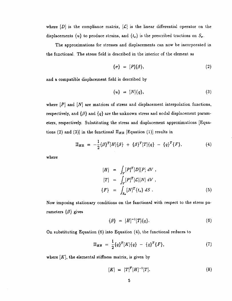
where [D] is the compliancematrix, [£] is the linear differential operator on the

displacements {u} to produce strains, and {to} is the prescribed tractions on S,.

The approximations for stresses and displacements can now be incorporated in

the functional. The stress field is described in the interior of the element as

(_} = [P](3}, (2)

and a compatible displacement field is described by

(,,} = [Nl(q}, (3)

where [P] and [N] are matrices of stress and displacement interpolation functions,

respectively, and {3} and {q} are the unknown stress and nodal displacement param-

eters, respectively. Substituting the stress and displacement approximations [Equa-

tions (2) and (3)] in the functional HHR [Equation (1)] results in

1

IIHR - 2[13}r[H]{fl} + {fl}T[T]{q} -- {q}T{F}, (4)

where

[HI = /v[PIr[D][P] dV ,

[T] = /v[pIT[£I[N] dV ,

{F} = /s[N]r{to} dS. (5)

Now imposing stationary conditions on the functional with respect to the stress pa-

rameters {fl} gives

{3} -[H]-I[TI{q}. (6)

On substituting Equation (6) into Equation (4), the functional reduces to

HHR = _{q}r[Kl{q} - (q}r{F},

where [K], the elemental stiffness matrix, is given by

(7)

[KI = [Tlr[H]-I[T]. (8)

5

Imposing the stationary conditions on the functional with respect to nodal displace-

ment unknowns {q}, results in a system of linear algebraic equations of the form

[K]{q} = {F}. (9)

Finite Element Approximations

Displacement Field

In the present paper, the Allman-type shape functions are used. However, the

formulation is direct rather than forming the stiffness matrix of an 8-node element

and then condensing it to a 4-node element stiffness matrix. All four edges of the

quadrilateral may be treated as 2-D beam elements with shear deformation, and the

general interpolation function for any typical edge can be expressed as in reference

[18]by

uO 1= +

vo 1= - +

5(1 + ,_)uj + (i - _2) (8.j- 8.i),

1 Azi(1 ___2)(Ozj_O,,i)5(1 + _)vj 8 (10)

and

where i = 1,2,3,4 and j = 2,3,4, 1 in that order. As mentioned earlier, the drilling

rotations are not interpolated independently. The out-of-plane displacement and out-

of-plane rotations are given by

to° = 5(1- _)w, + (i+ _)wj

Azi .

+ ---ff---(l- _') (euj -8tji )

iOu = 5(1-_)8vi + (l+_)8uj.

Ayi

S (1 - ,_2) (Szj - 8xi),

(11)

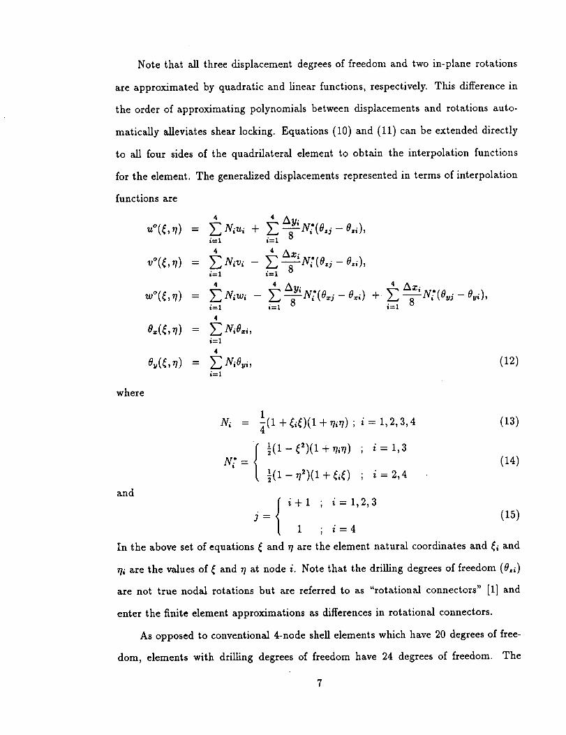
Note that all three displacement degrees of freedom and two in-plane rotations

are approximated by quadratic and linear functions, respectively. This difference in

the order of approximating polynomials between displacements and rotations auto-

matically alleviates shear locking. Equations (10) and (11) can be extended directly

to all four sides of the quadrilateral element to obtain the interpolation functions

for the element. The generalized displacements represented in terms of interpolation

functions are

where

and

1

N_ = 3(1+_,_)(1 +_?,T]); i= 1,2,3,4

½(1- _2)(I + _/17/) ; i= 1,3N.

{(1-_/2)(1+_i_) ; i=2,4

(13)

(14)

i+1 ; i=1,2,3j = (15)

1 , i=4

In the above set of equations _ and 7/are the element natural coordinates and _i and

r/i are the values of _ and _? at node i. Note that the drilling degrees of freedom (8,1)

are not true nodal rotations but are referred to as "rotational connectors" [1] and

enter the finite element approximations as differences in rotational connectors.

As opposed to conventional 4-node shell elements which have 20 degrees of free-

dom, elements with drilling degrees of freedom have 24 degrees of freedom. The

membrane part of the element has 12 degrees of freedom. Associated with these 12

degrees of freedom are 12 independent deformation modes. Three of these modes

are rigid-body modes and three other modes represent constant strain states. Of the

remaining six modes, five represent higher-order strain states and the last mode is

a spurious zero-energy mode. The spurious zero-energy mode associated with this

formulation is caused by the drilling rotations or rather the rotational connectors.

Note from Equations (10),(11) and (12) that the differences in rotations, and not the

drilling rotations themselves, enter the interpolation functions [see Equation (12)].

One of the four rotational differences is dependent on the other three rotational dif-

ferences, and hence, there are only three independent rotational degrees of freedom.

This produces a rank deficiency in the stiffness matrix and leads to a spurious zero-

energy mode. This spurious mode is associated with a state of zero nodal in-plane

displacements and equal nodal in-plane rotations.

However, this mode can be suppressed easily. MacNeal and Harder [16] eliminate

this mode by adding an energy penalty to the stiffness matrix. The energy penalty is

defined in terms of the weighted average of the differences between corner rotations

and the rotation at the center of the element. The rotation at the center of the element

is obtained by evaluating the skew-symmetric part of the displacement gradient at

the center of the element. A simpler way to eliminate this spurious mode, but which

calls for the awareness of any user of the finite element, is to prescribe the value of the

in-plane rotation at one node in the entire domain being analyzed. This will remove

the rank deficiency in the membrane part of the stiffness matrix.

The bending part of the element also has 12 degrees of freedom. Similar to

the membrane part, 12 independent deformation modes are associated with these 12

degrees of freedom. Three modes represent rigid-body modes, five modes represent

constant strain states, the remaining four modes represent higher-order strain states.

A spurious mode similar to the one in the membrane part does not occur here, though

the interpolation function for out-of-plane displacement w [Equation (11)] contains

out-of-plane (bending) rotational differences. In the membrane part, the rotational

degrees of freedom, as rotational differences, enter the formulation through the inter-

polation functions for in-plane displacements and not independently. However, in the

bending part, the out-of-plane rotations enter the formulation both independently

[2_ and 3 ra of Equation (11)] and through the interpolation function for w. Thus,

the bending part of the stiffness matrix is not rank deficient.

Assumed-Stress Field

In general, the selection of stress field approximation is governed by a few

conditions and guidelines [20] such as

• the satisfaction of equilibrium equations,

• interelement traction reciprocity,

• invariance and completeness of polynomial expansion, and

• spurious zero-energy modes.

In earlier hybrid models based on the principle of minimum complementary en-

ergy [21], the assumed-stress field satisfied equilibrium equations exactly, and conse-

quently the stress field was expanded in Cartesian coordinates. However, in the hybrid

formulations such as the present one, the assumed-stress field can be expanded in el-

ement natural-coordinate basis and the equilibrium equations need not be satisfied

a priori. In any case, the equilibrium equations are satisfied in a variational sense.

The invariance of the assumed-stress field could be achieved by having a complete

polynomial expansion [20]. However, the expansion of assumed-stress field in element

natural-coordinate basis provides a way to achieve the necessary invariance property

to the approximations.

Finally, the chosen stress field should produce no spurious zero-energy modes. Let

No be the number of independent stress parameters in the stress field approximations;

9

let Nd be the number of deformation modes associated with the element; let Nr be

the number of rigid-body modes associated with the element. In order to suppress

each independent deformation mode, it is necessary that a corresponding stress term

exists such that the deformation mode does not produce zero strain energy. As

such, each independent stress parameter should suppress one non-trivial independent

deformation mode [20, 22]. That is,

/v._> (lvd - lvr). (16)

While this statement sets a lower bound on N,, a definitive statement regarding the

upper bound on N0 cannot be made here. In this context, it is useful to define a ratio

'a' given by

N°a - Na - N," (17)

Based on Equation (16), it is clear that a > 1. At this stage, a stress field that is de-

scribed by a complete polynomial expansion in element natural-coordinate basis and

that does not satisfy equilibrium equations a priori might appear suitable. However,

it has been observed that a very high value of a produces a very stiff element [23].

Fraejis de Veubeke's limitation principle [25] states that when a complete indepen-

dent stress field that does not satisfy equilibrium equations a priori is assumed, the

hybrid element would reduce to a fully integrated displacement-based element. One

way to overcome this is to impose additional constraints by enforcing equilibrium

in the variational statement using Lagrange multipliers [3]. The lower bound on a

in mixed/hybrid formulations is stated mathematically by the inf - sup condition,

popularly known as the LBB condition [24].

In the present approach the assumed-stress field is not complete, and the equi-

librium equations are satisfied exactly for regular (rectangular) element shapes. The

stress field for the membrane part is assumed to be

= #, + + &,1 + #s,7:,

I0

(18)

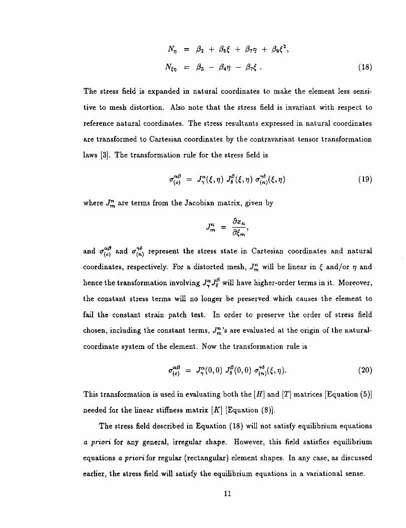
The stress field is expanded in natural coordinates to make the element less sensi-

tive to mesh distortion. Also note that the stress field is invariant with respect to

reference natural coordinates. The stress resultants expressed in natural coordinates

are transformed to Cartesian coordinates by the contravariant tensor transformation

laws [3]. The transformation rule for the stress field is

o'(c) = , o'(,_)(,_,r/) (19)

where d_ are terms from the Jacobian matrix, given by

J2-

'_ and ,y6and o'(e) cr(,,) represent the stress state in Cartesian coordinates and natural

coordinates, respectively. For a distorted mesh, d_ will be linear in _ and/or 7/and

hence the transformation involving _" _d._ d] will have higher-order terms in it. Moreover,

the constant stress terms will no longer be preserved which causes the element to

fail the constant strain patch test. In order to preserve the order of stress field

chosen, including the constant terms, d_'s are evaluated at the origin of the naturM-

coordinate system of the element. Now the transformation rule is

"_ " (.),_,,7). (2o)%) = J._(o,o)J/(O,O)_ _

This transformation is used in evaluating both the [HI and [T] matrices [Equation (5)]

needed for the linear stiffness matrix [g] [Equation (8)].

The stress field described in Equation (18) will not satisfy equilibrium equations

a priori for any general, irregular shape. However, this field satisfies equilibrium

equations a priori for regular (rectangular) element shapes. In any case, as discussed

earlier, the stress field will satisfy the equilibrium equations in a variational sense.

11

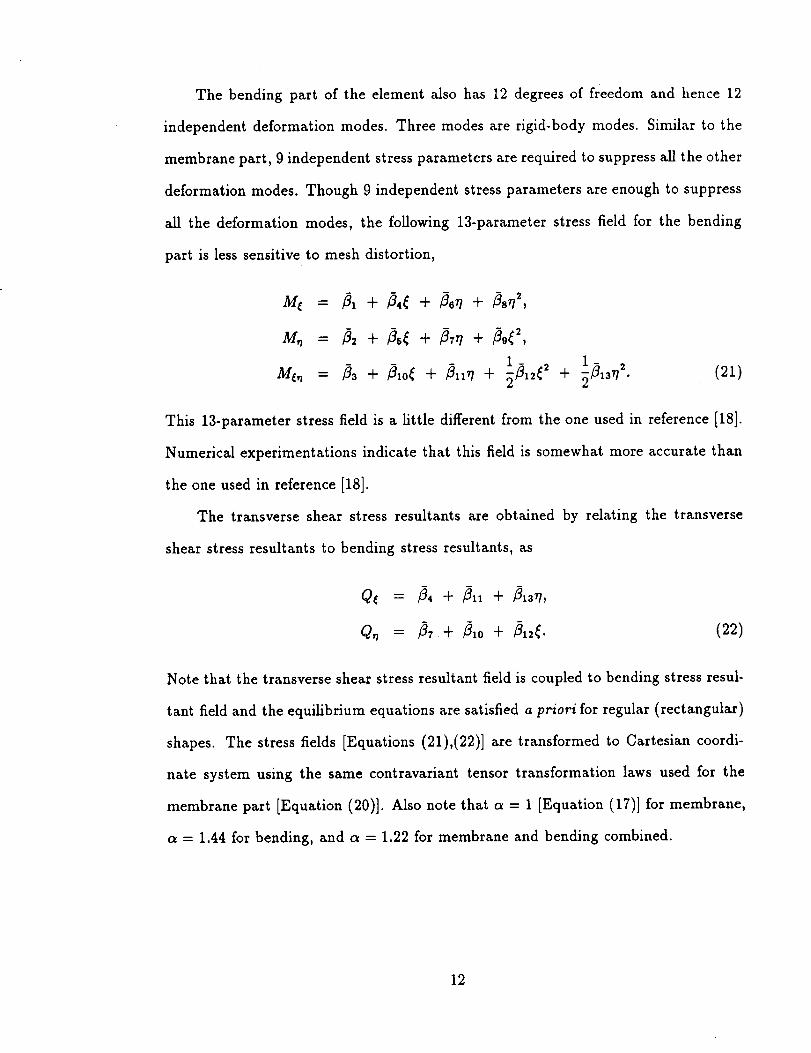
The bending part of the element also has 12 degrees of freedom and hence 12

independent deformation modes. Three modes are rigid-body modes. Similar to the

membrane part, 9 independent stress parameters are required to suppress all the other

deformation modes. Though 9 independent stress parameters are enough to suppress

all the deformation modes, the following 13-parameter stress field for the bending

part is less sensitive to mesh distortion,

M_ = 3, + 3,_ + 3s_ + 38_2,

1- 2

i_, = _3 + _1o_+ _11_+ _1- 2

+ _3_ • (21)

This 13-parameter stress field is a httle different from the one used in reference [18].

Numerical experimentations indicate that this field is somewhat more accurate than

the one used in reference [18].

The transverse shear stress resultants are obtained by relating the transverse

shear stress resultants to bending stress resultants, as

Q, = _7 + _10 + 3_. (22)

Note that the transverse shear stress resultant field is coupled to bending stress resul-

tant field and the equilibrium equations are satisfied a priori for regular (rectangular)

shapes. The stress fields [Equations (21),(22)] are transformed to Cartesian coordi-

nate system using the same contravariant tensor transformation laws used for the

membrane part [Equation (20)]. Also note that a = 1 [Equation (17)] for membrane,

a = 1.44 for bending, and a = 1.22 for membrane and bending combined.

12

Geometric Stiffness Matrix

The geometric stiffness or initial stress matrix is derived by using the full nonhnear

Green-Lagrange strain tensor

10ul Ouj Ouk Ouk(23)

Using Reissner-Mindlin kinematic assumptions and retaining the nonhnear terms only

for the membrane strains, the following relations result. The strains are written as

(24)

where {e°} are the membrane strains, {to} are the bending strains, and z is the

coordinate in the direction through the thickness of the plate or shell. The membrane

strains are written as

{¢} = {4} + {_?VL} (25)

where the linear part is given by

o = ovo/oy , (26){4} = _ o,,°lay + Ov°lax

E.zy

and the nonlinear part is given by

(--__) + + ' . (27)Ow" Ow"

-_ Dz ay Dx Dy

The bending strains are computed using the changes in curvature by

{,_} = ,_ = -oo./oy . (28)_.v OOu/ Oy - OO../ Oz

The transverse shear strains are given by

7_: = -o: + Ow°lOy "

13

The generalizedHeUinger-Reissnerfunctional including the nonlinearstrains can

be written as

IIHR --1

(30)

where {_r0} is the prescribed pre-buckling stress state. Upon substitution of the

displacement and stress approximations, Equation (30) reduces to

IIHR = --21-{j3}r[H]{fl} + {fl}T[Tl{q} -- {q}r{F} + _{q}T[K,,]{q}, (31)

where the element geometric stiffness matrix [K_] is given by

[K_] = /A[N]T[G]T[S][G][N] dA (32)

and

[G]

0.

0

0

where cgz = OIO_ and Ou = alOy.

0 0 0 0 0

0 0 0 0 0

o. o ooo

o oooo o ozooo

o o o ooo

The matrix IS], which corresponds to the pre-

buckling stress state, consists of membrane stress resultants which are either pre-

scribed or evaluated from a linear static stress analysis. It is given by

S 0 0][S] = 0 S 0 (33)

0 0 S

where

S

Consistent Mass Matrix

In linear free vibration analysis, it is assumed that the system is undamped and there

are no external forces. The HeUinger-Reissner functional [Equation (1)] with the

14

kinetic energycontribution can be written as

2 (34)

wheredots (.) over u indicate time derivatives. Upon substitution of stress field and

displacement field approximations, Equation (34) reduces to

where the consistent mass matrix [Me], representing the inertia of the system, is given

by

and

where

[Mc] = /A[N]T[#][N] dA (36)

[P]_×s

rno 0 0 0 ml

0 mo 0 -mr 0

0 0 mo 0 0

0 -ml 0 m2 0

ml 0 0 0 m2

, (37)

h

mo=f_: dz,2

h

ml-L..d.,2

h

Lm2 = pz 2 dz .2

(38)

and p is the mass density.

Numerical Results

The element described herein was developed and implemented within the framework

of NASA Langley Research Center's computational structural mechanics testbed

COMET [26] using the generic element processor template [27]. The element will

be referred to herein as A4S1.

15

The proper selection of displacement and stress fields has automatically elimi-

nated spurious zero-energy modes and locking in the present element and has made

the element invariant with respect to reference coordinates. However, the element

still needs to be validated with regard to its convergence and its sensitivity to mesh

distortion. MacNeal and Harder [28] have collected and proposed a standard set of

problems to test and validate a new element. The element's performance is observed

by analyzing these problems and a few other classical problems. The results are com-

pared with known theoretical solutions and other numerical solutions. Other 4-node

quadrilateral shell elements used for comparison are briefly described in Appendix A.

Consistent units have been used throughout the analyses.

Patch Test

This test was originally proposed by Irons [13] to establish the convergence of

an element. The patch test as shown in Figure 1 involves a specific mesh of distorted

elements with specified applied displacements that result in a constant state of either a

membrane or bending stress field. It is now widely recognized that an element should

pass the patch test, failing which, its convergence will not be assured. A4S1 passes

both the membrane and bending patch tests. The recovered strains and stresses are

exact.

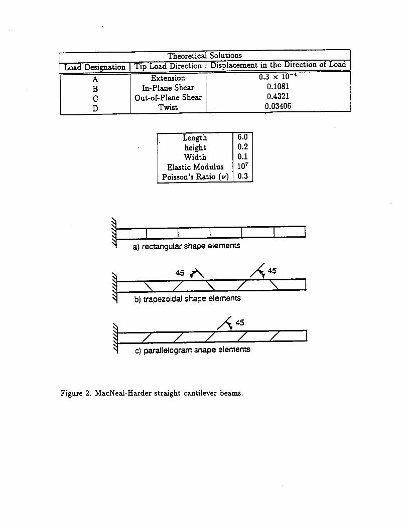
MacNeal-Harder Straight Cantilever Beam

This test case was proposed by MacNeal and Harder [28]. The capability of the

element to handle constant and linearly varying strains and curvatures is tested by

applying appropriate unit loads at the free end. The beam is modeled by a 6 x 1

mesh. It is discretized using rectangular-, trapezoidal- and parallelogram-shaped

elements. The element's sensitivity to mesh distortion is studied and compared with

other elements. The finite element discretizations and the exact solutions [28] are

16

shown in Figure 2. The theoretical result for twist (load D) is 0.03406 as reported

in Timoshenko and Goodier [29]. However, reference [28] reports the solution to

be 0.03028. Analysis with successively refined meshes converged to 0.03385 which

is much closer to Timoshenko and Goodier solution [29], and hence this solution is

used here for normalization. The normalized results given in Table I indicate that

the elements predict good results for rectangular-shaped elements and the results

deteriorate for the two distorted mesh cases. However, A4S1 performs very well and

can handle distorted mesh configurations effectively.

• Remark 1: Attention is drawn to the case of in-plane shearing load (load B),

particularly in distorted mesh configurations. 4_ANS, 4_HYB, and QUAD4

perform badly. The advantage of drilling degrees of freedom is evident from

the superior performance of the present element, the performance of Q4S, and

a relatively modest improvement shown by 4_STG.

• Remark 2:A4S1 has shown improvement over AQR8 and AQD4 for the twist

(load D), and this is attributed to the modified bending stress field.

• Remark 3: The rotational degrees of freedom by virtue of their presence in

the element displacement shape functions, enter into the calculations of work-

equivalent nodal loads. Hence, the in-plane and out-of-plane loads at the beam

tip correspond to both statically equivalent loads and the work-equivalent loads

including moments corresponding to the rotational degrees of freedom.

Twisted Cantilever Beam

This test case involves a straight cantilever beam twisted 900 over its length [28].

The twisted beam shown in Figure 3 is modeled by 12 elements along the length and

2 elements across the width. Each element has a 7.50 warp and the effect of this warp

on the element's performance is studied. The results tabulated in Table II indicate

that A4S1 performs very well, but does not show improvement over AQR8 and AQD4.

While 4_STG and QUAD4 perform well, 4_.ANS and 4_HYB do not perform very well.

17

Curved Cantilever Beam

The curved cantilever beam formed by a 900 circular arc is shown in Figure 4.

The loading consists of in-plane shear and out-of-plane shear at the tip [28]. The

results tabulated in Table III indicate that the new element performs very well. Again

A4S1 has shown a modest improvement over AQR8 and AQD4 for the out-of-plane

shear (load C) and this is again attributed to the improved bending stress field.

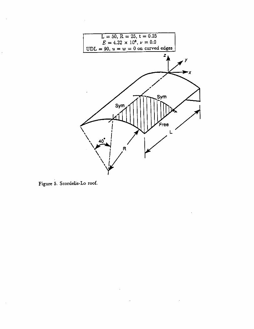
Scordelis-Lo Roof

The Scordelis-Lo roof [30] is a singly curved shell structure (see Figure 5).

The shell has a gravity load or a uniform dead load (UDL), and the parameter of

interest is the vertical displacement at the mid-point of the free edge (point A in

Figure 5). Though the theoretical value used in reference [30] is 0.3086, the value

used by MacNeal and Harder [28] is 0.3024. This latter value is used for normalization

here. Due to the symmetry of the structure and loading, only one quadrant of the shell

is modeled. The convergence behavior is studied for meshes from 2 × 2 to 10 × 10 and

is tabulated in Table IV. The A4S1 element shows a rapid and monotonic convergence.

Morley's Spherical Shell

The spherical shell is doubly curved (see Figure 6) and the equator of the shell is

chosen to be a free edge. Hence, the problem reduces to a hemisphere with four point

loads alternating in sign at 900 intervals along the equator. An 18 ° hole has been

introduced at the top of the hemisphere to avoid having to model the pole [28]. The

theoretical solution for displacement at the point of load and in the direction of the

load is reported as 0.094 in reference [28] and it is used here for normalization. Only

a quadrant of the shell is modeled. Convergence is studied for meshes from 2 × 2 to

12 x 12 and the results are tabulated in Table V. While 4..ANS and QUAD4 seem

18

to show a very rapid convergence, A4S1, AQR8, AQD4, and 4_STG exhibit a slow

convergence. Note that even for a 12 x 12 mesh, A4S1 shows an 8.4% error.

Remark 4: The present problem involves significant contribution from both

membrane and bending strains to the radial displacement at the points of

loading. The reason attributed for the slow convergence of the elements with

drilling rotations [16] is that the stiffness of the shell is increased by membrane-

bending coupling arising out of the faceted geometric approximation of the

shell. This coupling is actually the coupling between drilling rotations and

beading rotations due to the changes in slopes at element interfaces (because

of faceted representation).

Remark 5: Furthermore, the membrane-bending coupling may be amplified by

the fact that the drilling rotations are not true rotations, but are rotational

connectors. An independent drilling rotation entering the formulation either

through the variational statement or through the kinematics may increase the

flexibility of the discretized shell.

Isotropic Square Plate

The classical plate bending problem of a clamped, isotropic square plate sub-

jected to a concentrated load at its center is analyzed. The convergence behavior,

the effect of mesh distortion, and the effect of varying the thickness of the plate are

studied. The geometry of the plate and its properties are shown in Figure 7. The

maximum defection at the center of the plate, as calculated in reference [31] using

the Ritz approximation, is given by

p_2

= 0.0056--D-- (39)

where D is the flexural rigidity of the plate, P is the apphed concentrated load for

the full plate, and a is the side length of the plate. The central deflections obtained

from the finite element analyses are normalized with respect to the value calculated

from Equation 39.

The convergence behavior shown in Figure 7 indicates that A4S1 converges

rapidly and monotonically. Next, the analysis is carried out using a distorted 7x7

mesh. The center of the quarter plate is fixed and the nodes immediately adjacent to

19

the central node are rotated from 0 to 45 degrees. The boundary nodes are also fixed.

From Figure 8, the mesh distortion is shown to have the least effect on A4S1. Again

A4S1 offers a modest improvement over AQR8 and AQD4. As mentioned earlier, the

consistent interpolation order between the transverse displacement and out-of-plane

rotations eliminates shear locking in A4S1. To confirm this with numerical valida-

tion, the effect of decreasing the thickness of the plate on the element's performance

is studied. The length-to-thickness ratio (defined as a/h) is varied from 10 to 10,000.

None of the elements lock at high length-to-thickness ratio. Representative results

for two elements are shown in Figure 9.

Pear-Shaped Cylinder

This is an extremely interesting problem because of its continually varying ge-

ometry. The cross-section of the cylinder is shown in Figure 10, which supposedly is a

representation of an early space shuttle fuselage configuration. The sheU is isotropic

with a uniform thickness of 0.01 inches. Only one quarter of the cylinder is modeled

due to the symmetry of the structure. Symmetry boundary conditions are imposed

on three edges and a uniform end shortening is applied to the simply supported edge.

The analysis is carried out using three different meshes: 4 x 23 (92 nodes, 66 ele-

ments), 5 x 34 (170 nodes, 132 elements), and 7 x 51 (357 nodes, 300 elements),

where n x m refers to rt nodes along the length of the cylinder and m nodes along

the half-cylinder circumference. However, the solution reported here is for the 7 × 51

mesh, where the solutions converge.

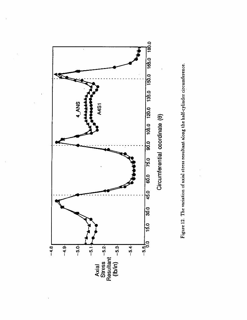
One of the earliest available numerical analyses on this problem was performed

by Hartung and Ball [32]. The variation of radial displacements and the axial stress

resultants with 0 measured counter-clockwise from the top, are shown in Figures 11

and 12, respectively. Results of 4_ANS and A4S1 are very close. Further comments

on the accuracy of the solution cannot be made here due to the lack of linear static

20

analysisdata on this problem. However, this problem has been an attractive target

for nonlinear analyses and elastic shell collapse studies, due to its complex nonlinear

collapse behavior. Herein a linear elastic buckling analysis is carried out on the

cylinder. The buckling loads for two modes are presented in Table VI and the buckling

mode shapes are shown in Figure 13. Since there are no analytical solutions available

for comparison, the results are normalized with respect to converged solutions of a

9-node assumed natural strain element (9_ANS) [26, 33]. The present element and

4_STG which contain the drilling degree of freedom, predict lower buckling loads

compared to 4_ANS.

Rectangular Plate

This problem is analyzed to validate the element's capability to handle linear

buckling and free vibration problems. This is a classical problem for which theo-

retical solutions exist. The rectangular plate [see Figure 14] is isotropic and simply

supported on all sides. The plate is subjected to a uniform uniaxial compression and

a biaxial compression [see Figure 14(a) and 14(5), respectively]. Only a quarter of

the plate is discretized, with a 5 x 8 mesh [shaded region in Figure 14(a) and 14(b)].

The linear buckling analysis is performed with the pre-buckling stress state consist-

ing of stresses computed from a linear static analysis. The results are tabulated in

Table VII and VIII, where m and n refer to the number of half waves in X and Y

directions, respectively. The results are normalized with respect to the theoretical

solutions reported in reference [34]. A4S1 predicts quite accurate buckling loads and

again, A4S1 and 4_STG predict lower buckling loads than 4_.ANS. The plate is also

subjected to an uniform shear and the full plate is discretized with a 5 x 8 mesh [see

Figure 14(c)]. The results are shown in Table IX. A4S1 predicts a lower and more

accurate buckling load than 4_ANS.

21

A free vibration analysis is carried out on the plate in its unstressed state. The

results are tabulated in Table X, where m and n refer to the number of half waves

in X and Y directions, respectively. The results are normalized with respect to the

theoretical solutions reported in reference [34]. A4S1 gives quite accurate natural

frequencies, but 4_HYB seems to have performed marginally better.

Axially Compresse d Cylinder

A cylindrical shell with simply supported edges is subjected to an uniform axial

compression (see Figure 15). The prestress state is computed from a linear stress

analysis of the axially compressed cylinder. Note that this prestress state is not

exactly constant due to the simply supported boundaries, which prevents the shell

from uniformly expanding in circumferential direction. Another interesting feature

Of this problem is the closely packed eigenvalues and the corresponding considerably

different mode shapes. Modeling the entire cylinder is computationally intensive and

hence only a 15-degree sector and one tenth of the length of the cylinder, sufficient to

capture the lowest mode, is modeled. Symmetric boundary conditions are employed

on all edges except the loaded edge which is simply supported. A convergence study

is done for meshes N x N, where N (number of nodes per side) ranges from 3 to 9

(see Figure 15). A4S1 and 4_STG show a better convergence than 4_ANS. The first

two mode shapes of this discretization are shown in Figure 16.

Cylindrical Shell

An octant of a cylindrical shell (see Figure 17) is analyzed for the free vibrational

characteristics of the cylindrical shell. To capture the correct modes, symmetric and

anti-symmetric boundary conditions are defined for the edge BC. Edge AB is simply

supported and Edges AD and DC are in the symmetric planes. The results are

compared with the theoretical solutions reported in reference [35] and are tabulated

22

in Table XI. The mesh refers to number of nodes in the circumferential direction by

number of nodes in the axial direction. A4S1 and 4_HYB converge to the theoretical

solution. The vibration mode shapes are shown in Figure 17.

Conclusions

Numerical results indicate that the element developed in this paper is devoid of the

usual deficiencies of 4-node shell elements. Though the element has one spurious

zero-energy mode, this mode can be suppressed easily by prescribing the value of

in-plane normal rotation at one node in the entire finite element model. It has been

shown that the element is nearly insensitive to mesh distortion, does not lock, and

has desirable convergence and invariance properties. The element has also performed

very well for buckling and free vibration analyses.

Acknowledgment

The research reported herein was sponsored by NASA Langley Research Center and

Dr. Alexander Tessler was the technical monitor. The first and third authors were

sponsored by NASA Grant NAG-l-1374, and the second author was sponsored by

NASA Contract NAS1-19317.

23

[1]

[2]

[3]

[4]

[5]

[6]

[7]

[sl

[9]

[10]

[11]

[12]

References

Allman, D.J., "A Compatible Triangular Element Including Vertex Rotations for

Plane Elasticity Analysis", Computers and Structures, Vol. 19, 1984, pp. 1-8.

Bergan, P.G., and Fehppa, C.A., "A Triangular Element with Rotational Degrees

of Freedom", Computer Methods in Applied Mechanics and Engineering, Vol. 50,

1985, pp. 25-69.

Pian, T.H.H., "Evolution of Assumed Stress Hybrid Finite Element", in Ac-

curacy, Reliability and Training in FEM Technology, Proceedings of the Fourth

World Congress and Exhibition on Finite Element Methods, Edited by John

Robinson, Interlaken, Switzerland, 1984, pp. 602-619.

Tan, H.Q., Chang, T.Y.P., and Zheng, D., "On Symbolic Manipulation and

Code Generation of a Hybrid Three-dimensional Solid Element", Engineering

with Computers, Vol. 7, 1991, pp. 47-59.

Cook, R.D., Malkus, D.S., and Plesha, M.E., Concepts and Applications of Finite

Element Analysis, Third Edition, John Wiley and Sons Inc., New York, 1989.

Zienkiewicz, O.C., The Finite Element Method, Fourth Edition, Vol. 1, McGraw-

Hill, New York, 1988.

Reissner, E.,"A Note on Variational Principles in Elasticity", International Jour-

nal of Solids and Structures, Vol. 1, 1965, pp. 93-95.

Hughes, T.J.R., and Brezzi, F., "On Drilling Degrees of Freedom", Computer

Methods in Applied Mechanics and Engineering, Vol. 72, 1989, pp. 105-121.

Ibrahimbegovic, A., Taylor, R.L., and Wilson, E.L., "A Robust Quadrilateral

Membrane Finite Element with Drilling Degrees of Freedom", International

Journal for Numerical Methods in Engineering, Vol. 30, 1990, pp. 445-457.

Ibrahimbegovic, A., and Wilson, E.L., "A Unified Formulation for Triangular and

Quadrilateral Flat Shell Finite Elements with Six Nodal Degrees of Freedom",

International Journal for Numerical Methods in Engineering , Vol. 7, 1991, pp.

1-9.

Iura, M., and Atluri, S.N., "Formulation of a Membrane Finite Element with

Drilling Degrees of Freedom", Computational Mechanics, Vol. 9, 1992, pp. 417-

428.

Robinson, J., "Four-Node Quadrilateral Stress Membrane Element with Rota-

tional Stiffness", International Journal for Numerical Methods in Engineering,

Vol. 16, 1980, pp. 1567-1569.

24

[13]

[14]

[15]

[16]

[17]

[18]

[19]

[2o]

[21]

[22]

[23]

[24]

[25]

[26]

Irons, B.M., and Ahmad, S., Techniques of Finite Elements, Ellis Horwood Ltd.,

Chichester, West Sussex, 1980.

Cook, R.D., "On the Allman Triangle and a Related Quadrilateral Element",

Computers and Structures, Vol. 22, 1986, pp. 1065-1067.

AUman, D.J., "A Quadrilateral Finite Element Including Vertex Rotation for

Plane Elasticity Analysis", International Journal for Numerical Methods in En-

gineering, Vol. 26, 1988, pp. 717-730.

MacNeal, R.H., and Harder, R.L., "A Refined Four-Noded Membrane Element

with Rotational Degrees of Freedom", Computers and Structures, Vol. 28, 1988,

pp. 75-84.

Yunus, S.H., Saigal, S., and Cook, R.D., "On Improved Hybrid Finite Elements

with Rotational Degrees of Freedom", International Journal for Numerical Meth-

ods in Engineering, Vol. 28, 1989, pp. 785-800.

Aminpour, M.A., "An Assumed-Stress Hybrid 4-Node Shell Element with

Drilling Degrees of Freedom", International Journal for Numerical Methods in

Engineering, Vol. 33, 1992, pp. 19-38.

Aminpour, M.A., "Direct Formulation of a Hybrid 4-Node Shell Element with

Drilling Degrees of Freedom", International Journal for Numerical Methods in

Engineering, Vol. 35, 1992, pp. 997-1013.

Pian, T.H.H., Chen, D.P., and Kang, D.,"A New Formulation of Hybrid/Mixed

Finite Element", Computers and Structures, Vol. 16, 1983, pp. 81-87.

Pian, T.H.H., "Derivation of Element Stiffness Matrices by Assumed Stress Dis-

tribution", AIAA Journal, Vol. 2, 1964, pp. 1333-1336.

Pian, T.H.H., and Chen, D.P., "On the Suppression of Zero Energy Deformation

Modes", International Journal for Numerical Methods in Engineering, Vol. 19,

1983, pp. 1741-1752.

Kang, D., Hybrid Stress Finite Element Method, Ph.D. Dissertation, Mas-

sachusetts Institute of Technology, Cambridge, MA, 1986.

Brezzi, F., and Fortin, M., Mized and Hybrid Finite Element Methods, Springer-

Verlag, New York, 1991.

Fraejis de Veubeke, B., "Displacement and Equilibrium Models in the Finite Ele-

ment Method", Zienkiewicz, O.C., and Hohster, G.S., (Editors), Stress Analysis,

Wiley, London, 1965, pp. 145-197.

Stewart, C.B., "The Computational Structural Mechanics Testbed User's Man-

ual", NASA TM-IO0644 (updated), 1990.

25

[27]

[28]

[29]

[3o]

[31]

[32]

[33]

[34]

[35]

[36]

[37]

Stanley, G.M., and Nour-Omid, S.,"The Computational Structural Mechanics

Testbed Generic Structural Element Processor Manual", NASA CR-181728,

1990.

MacNeal, R.H., and Harder, R.L., "A Proposed Standard Set of Problems to

Test Finite Element Accuracy", Finite Elements in Analysis and Design, Vol. 1,

1985, pp. 3-20.

Timoshenko, S.P., and Goodier, J.N., Theory of Elasticity, Third Edition,

McGraw-Hill, New York, 1970.

Scordelis, L.O., and Lo, K.S., "Computer Analysis of Cylindrical Shells", Journal

of American Concrete Institute, Vol. 61, 1969, pp. 539-561.

Timoshenko, S.P., and Woinowsky-Krieger, S., Theory of Plates and Shells, Sec-

ond Edition, McGraw-Hill, New York, 1959.

Hartung, R.F., and Ball, R.E., "A Comparison of Several Computer Solutions to

Three Structural Shell Analysis Problems", AFDL TR-73-15, Air Force Flight

Dynamics Laboratory, Dayton, OH, April 1973.

Park, K.C., and Stanley, G.M., "A Curved C O Shell Element Based on Assumed

Natural-Coordinate Strains", ASME Journal of Applied Mechanics, Vol. 108,

1986, pp. 278-290.

Stewart, C.B., "The Computational Structural Mechanics Testbed Procedures

Manual", NASA CR-1006_6, 1990.

Forsberg, K., "Influence of Boundary Conditions on the Modal Characteristics

of Thin Cylindrical Shells", AIAA Journal, Vol. 2, 1964, pp. 2150-2157.

Almroth, B.O., Brogan, F.A., and Stanley, G.M., "Structural Analysis of Gen-

eral Shells", Vol. II, User's Introduction for STAGSC-1 Computer Code, Report

Number: LMSC-D633873, Lockheed Palo Alto Research Laboratory, Palo Alto,

CA, December 1982.

Aminpour, M.A., "Assessment of SPAR Elements and Formulation of Some Ba-

sic 2-D and 3-D Elements for Use with Testbed Generic Element Processor",

Proceedings of NASA Workshop on Computational Structural Mechanics - 1987,

NASA CP-10012, Part 2, Nancy P. Sykes (Editor), 1989, pp. 653-682.

26

Appendix A

EX47(ES1): A C °, isoparametric, assumed natural-coordinate strain element, devel-

oped by Park and Stanley [33]. The element is not invariant with respect to

reference coordinates and does not pass the patch test. This element will be

referred to as 4_ANS.

QUAD4: A 4-node isoparametric shell element with selective reduced integration [28].

This element is available in MSC/NASTRAN. Q4S, an improved version of

QUAD4, contains the drilling degree of freedom [16].

E410(ES5): A C 1, incompatible, displacement based element with drilling degrees of

freedom. The element kernels were extracted from the STAGS computer code

(Almroth et a1.[36]). The element uses cubic interpolation for the displacement

field. This element is not invariant and does not pass the patch test. This

element will be referred to as 4_STG.

EX43(ES4): A U °, isoparametric_ assumed-stress hybrid shell element with no drilling

degree of freedom. This element is invariant with respect to reference coordi-

nates and passes the patch test. This element was developed by Aminpour[37].

This element will be referred to as 4_HYB.

AQR8(ES8): An assumed-stress hybrid shell element with drilling degrees of freedom,

developed by Aminpour [18]. The formulation is based on Hellinger-Reissner

variational principle. The 4-node element is obtained from an "internal" 8-

node element.

AQD4(ES8): An assumed-stress hybrid shell element with drilling degrees of free-

dom, developed by Aminpour [19]. The formulation is based on modified

complementary energy principle and the stress field is expanded in Cartesian

coordinates.

27

Table

I.

II.

III.

IV.

V.

VI.

VII.

List of Tables

MacNeal-Harder straight cantilever beams.

MacNeal-Harder twisted cantilever beam.

MacNeal-Harder curved cantilever beam.

Scordelis-Lo roof.

Morley's spherical shell.

Linear buckling analysis of the pear-shaped cyhnder.

Linear buckhng analysis of the rectangular plate under uniaxial compression.

VIII. Linear buckling analysis of the rectangular plate under biaxial compression.

IX. Linear buckhng analysis of the rectangular plate under uniform shear.

X. Linear free vibration analysis of the rectangular plate.

XI. Linear free vibration analysis of the cyhndrical shell.

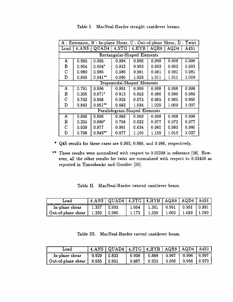
Table I. MacNeal-Harderstraight cantileverbeams.

A : Extension, B : In-plane Shear, C : Out-of-plane Shear, D :Twist

Load[4_ANS QUAD414_STG 4_HYB AQR8 AQD4 A4SI

Rectangular-Shaped Elements

A 0.995

B 0.904

C 0.980

D 0.856

0.995

0.904'

0.986

0.941"

0.994

0.915

0.986

0.680

0.996

0.993

0.981

1.023

0.998

0.993

0.981

1.011

0.998

0.993

0.981

1.011

0.998

0.993

0.981

1.009

Trapezoidal-Shaped Elements

A 0.761

B 0.305

C 0.763

D 0.843

0.996

0.071"

0.968

0.951 o"

0.991

0.813

0.925

0.683

0.999

0.052

0.075

1.034

0.998

0.986

0.965

1.029

0.998

0.986

0.965

1.009

0.998

0.986

0.969

1.007

Parallelogram-Shaped Elements

A 0.966

B 0.324

C 0.939

D 0.798

0.996

0.080"

0.977

0.945 o"

0.989

0.794

0.991

0.677

0.999

0.632

0.634

1.166

0.998

0.977

0.980

1.159

0.998

0.972

0.980

1.010

0.998

0.977

0.980

1.007

* Q4S results for these cases are 0.993, 0.988, and 0.986, respectively.

** These results were normalized with respect to 0.03208 in reference [28]. How-

ever, all the other results for twist are normalized with respect to 0.03406 as

reported in Timoshenko and Goodier [29].

Table II. MacNeal-Harder twisted cantilever beam.

Load 4_ANS QUAD4

In-plane shear 1.357 0.993

Out-of-plane shear 1.293 0.985

4_STG

1.054

1.173

4_HYB

1.361

1.359

AQR8

0.991

1.093

AQD4 IA4SI

0.991 0.991

1.093 1.093

Table III. MacNeal-Harder curved cantilever beam.

Load

In-plane shear 0.929

Out-of-plane shear 0.935

4_ANS QUAD4 4_STG 4_HYB AQR8

0.833

0.951

0.938

0.887

0.888

0.925

0.997

0.956

AQD4 IA4SI

0.996 0.997

0.956 0.970

Table IV. Scordelis-Loroof.

Mesh 4_ANS QUAD4 4_STG 4_HYB AQR82x2

4x4

6x6

8x8

i0 x 10

1.387

1.039

1.011

1.005

1.003

1.376

1.050

1.018

1.008

1.004

1.384

1.049

1.015

1.005

1.001

1.459

1.068

1.028

1.017

1.011

1.218

1.021

1.006

1.003

1.001

AQD4 [ A4S1

1.218 1.222

1.021 1.022

1.006 1.007

1.003 1.003

1.001 1.001

Table V. Morley's Spherical Shell.

Mesh

2x2

4x4

6x6

8x8

I0 x I0

12 x 12

4_ANS QUAD4 4_STG 4_HYB AQR8 IAQD4

0.968

1.018

1.001

0.995

0.993

0.992

0.972

1.024

1.013

1.005

1.001

0.998

0.338

0.519

0.841

0.949

0.978

0.988

1.032

1.093

1.060

1.040

1.027

1.020

0.382

0.227

0.432

0.681

0.835

0.914

I A4S1

0.381 0.425

0.226 0.231

0.432 0.433

0.680 0.682

0.835 0.838

0.914 0.916

Table VI. Linear buckling analysis of the pear-shaped cylinder.

Modes 9_ANS 4_ANS

1 4.393 1.021

2 6.483 1.032

4_STG 4_HYB

1.002 1.016

1.013 1.027

A4S1

1.013

1.016

Table VII. Linear buckling analysis of the rectangular plate under uniaxial

compression.

N;, N,,I N;Modes n Analytical 4_ANS 4_STG 4_HYBiA4S1

1 1 523.04 1.013 0.991 1.008 0.998

2 3 874.89 1.044 0.988 1.023 1.001

Table VIII. Linear buckling analysisof the rectangular plate under biaxial

compression (N. = Nu = N).

Modes m n

1 1 1

2 1 3

3 3 1

*

Analytical

188.29

730.58

1152.36

N/N"

4_ANS 4_STG 4AIYB I A4S1

1.010 0.995 1.005 0.998

1.047 0.981 1.027 1.003

1.153 0.998 1.095 1.020

Table IX. Linear buckling analysis of the rectangular plate under uniform shear.

ModesNx*y

Analytical 4_ANS 4_STG

1 3629.69 1.284 0.930

N_y

4_HYB ]A4SI

1.213 [ 0.989

Table X. Linear free vibration analysis of the rectangular plate.

Modes m n

1 1 1

2 1 3

3 3 1

Frequency

Q

Analytical 4_ANS

112.40 1.008

436.10 1.036

687.80 1.111

f/f°

4_HYB IA4S1

1.005 1.010

1.026 1.037

1.083 1.087

Table XI. Linear free vibration analysis of the cylindrical shell.

Number of circumferential waves = 6

Symmetric Mode 1

Theoretical [35]

w_ = 0.633 x 105

Mesh 4_ANS

25x9

31 x II

35 x 13

1.022

1.008

1.002

4_HYBIA4SI

1.013 1.021

1.000 1.009

0.995 1.005

Anti-symmetric Mode 1

Theoretical 35]

w_. = 0.581 x 10 s

4_ANS 4AtYB A4S1

1.028 1.010 1.026

1.009 0.995 1.012

1.002 0.988 1.005

Figure

1.

2.

3.

4.

5.

6.

7.

List of Figures

The patch test.

MacNeal-Harder straight cantilever beams.

MacNeal-Harder twisted cantilever beam.

MacNeal-Harder curved cantilever beam.

Scordelis-Lo roof.

Morley's spherical shell.

Convergence study for the isotropic square plate; a = 4, h = 0.001,

P= 100, E=107 , v=0.3.

8. The effect of mesh distortion (for a 7 × 7 mesh).

9. The effect of thickness change (for a 7 × 7 mesh).

10. The pear-shaped cylinder.

11. The variation of radial displacements along the half-cylinder circumference.

12. The variation of axial stress resultant along the half-cylinder circumference.

13. Buckling mode shapes for the pear-shaped cylinder.

14. Linear buckling analysis of the rectangular plate under (a) uniaxial

compression, (b) biaxial compression, and (c) uniform shear; length along the

X-direction = 15, length along the Y-direction = 20, E = 30 × 108, u = 0.3.

15. Convergence of the critical load for the axially compressed cylinder;

E=107 , v=0.3, R=36, L=100, I= 10, t=0.125, 8= 15 °.

16. Mode shapes corresponding to the lowest two critical loads

for the axially compressed cylinder.

17. Vibration mode shapes for the cylindrical shell; E = 107, v = 0.3,

p=0.1, R=10, t=0.1, h=5.

Location of Nodes

Node x y

1 0.04 0.02

2 0.18 0.03

3 0.16 0.08

4 0.08 0.08

[ a=0.12, b=0.24, t =0.001, E= 10 s,v=0.25 ]

Boundary Conditions Theoretical Solution

Membrane Patch Test

= 1o- (x + y/2)v = 10-_(=/2 + y)

N==N v= 1.333

N_ = 0.4

Bending Patch Test

w = 10-3(x 2 + xy + y_)/2

0= = 10-3(z/2 -+-y) M= = M r = -1.111 x 10-7

0_ = -10-s(z + y/2) Mzv = -3.333 x 10 -8

Y

b

_X

Figure 1. The patch test.

TheoreticalSolutions

Load Desigilation Tip Load Direction Displacement in the Direction of Load

A

B

C

D

Extension

In-PlaneShear

Out-of-PlaneShear

Twist

0.3 × 10-4

0.1081

0.4321

0.03406

Length

heightWidth

ElasticModulus

Poisson'sRatio (u)

6.0

0.2

0.i

107!0.31

i

I i I I Ia) rectangularshape elements

' X /' \ / 'Xb) trapezoidal shape elements

/_T 45

/ / / /c) parallelogram shape elements

d,/

Figure 2. MacNeal-Harder straight cantilever beams.

Theoretical Solutions

Tip Load Direction Displacement in the Direction of Load

In-Pla_e Shear 0.005424

Out-of-Plane Shear 0.001754

Length

Width

Depth

Elastic Modulus

Poisson's Ratio (v)

12.0

1.1

0.32

29.0 x I0e

0.22

Figure 3. MacNeM-H_der twisted cantilever beam.

Theoretical Solutions

Tip Load Direction Displacement in the Direction of Load

In-Plane Shear 0.08734

Out-of-Plane Shear 0.50220

Inner Radius 4.12 I

Outer Radius 4.32 1

Depth 0.10i

ElasticModulus i0z i

Poisson's Ratio (v) 0.25 1i

\

9O

P

Figure 4. MacNeal-Harder curved cantilever beam.

L = 50, i_. = 25, t = 0.25

E=4.32 x 108 ,v=0.0

UDL = 90, u = w = 0 on curved edges

Z

/lJ\,\/ t_

Figure 5. Scordelis-Lo roof.

Radius = i0.,Thickness - 0.04JE -- 6.825 x i0z, _,= 0.3

z

Sym !Sym

F= 1.0Y

F=I.IFree

Figure 6. Morley's spherical shell.

"I-

or)Z

G)nO°_

(I)O.

(2)

0z

oL_

G)

E

Z

uo!1oelIeOle.queo pez!lekUJON

II

II

o-_p

l-e

o"

0I=i

0

o4--I

0

t_ <_

I,.i

= I1.F,,_

q'In"

i̧ira(

+

I

>--r".,,mr.I

I.¢

I

_I ',"-q+.

,r,--

iii,

_- (/)Z

< <

iki,.3C

a0<C

I

I0 01 CO I'%

.,.- .,,- 0 C_ 0 0o'+.0

r,_

EIL'-,,

X

It.-,.

Id

I,,.i

I,.I

0

r_°+,.i

,,.c::u'J

I,l.,I

O

4.)I-i

t_°,-i

uo!_el_eE] leJJ,ueo pez!leU.UON

_l..c

q)

X

I-i

Q)

U

r_

Uo,M

0

a)

c_

oI==,

r_

uo!_el,Leo leJJ,ueo pez!leWJON

I R=I,L=O.3, t=O.OI IE = i07,u = 0.3 J

Figure 10. The pear-shaped cylinder.

(D

(/)

<:

J_GOqr'-

C_

j.r)c.O

0

T'-

h,B

oo 0

°_

0 c"

Q)

EC:) --I

°m

00

i,q-

C_

'0')

:0

-L5

c5

L)

L.

I--6o,,..t

L.

°_

0

c_u_

(J)

....q

l..i

0

0o_

_0°_

_-- (]) :_.0

z_ xt-_ -.-.-

I I I I I I I I

rr

U

U

U

0

0

°_

Mode 1

Ny / Ny (converged) = 1.013

Mode 2

Ny / Ny (converged) = 1.016

Figure 13. Buckling mode shapes for the pear-shaped cylinder.

(a)

Nx=I_ =1

(b) %

Y

Nxy= 1

(c)

Figure 14. Linear buckling analysis of the rectangular plate under (a) uniaxial

compression, (b) biaxial compression, and (c) uniform shear; length along theX-direction = 15, length along the Y-direction = 20, E = 30 x 10e, v = 0.3.

q

\

0

"0o_

(,_(D

,._"_ 0

ZwI,-,,

oI,..

(D,,C}

E

Z

..,¢.

coo

'U

v}

o II

H

o II

'J' C_

(P

..c:: w..,1

o e,o

o IIr...>

o

Discretized Model (9 x 9)

Mode 1

_.cr - 0.99892

Mode 2

_.cr -" 1.02980

Figure 16. Mode shapes corresponding to the lowest two critical loads

for the axially compressed cylinder.

Discretized Model (35 x 13)

X

l A

h

Z

Sym.

Symmetric Mode 1 Anti-symmetric Mode 1

_2= 0.636 x 105 _2__ 0.584 x 105

Figure 17. Vibration mode shapes for the cyhndrical shell; E = l0 T, v = 0.3,

p=0.1, R=I0, t =0.i, h=5.