Policy, Planning, and Rse"rach

WORKING PAPERS L f>S OO0 I

Trade Policy

Country Economics DepartmentThe World Bank

March 1988WPS 1

Imports Undera Foreign Exchange

Constraint

Cristian Moran

To estimate how adjustment packages will affect the flow ofimports, policymakers need to look beyond the traditional ex-planatory variables of gdp and real import prices. They mustfocus in addition on the availability of foreign exchange.

The Policy, Planning, and Research Cornpler distributes PPR Working Papers to disseminate the findings of work in progress and toencourage the exchange of ideas among Bank staff and all others interested in development issues. These papers carry the names ofthe authors, reflect only their views, and should be used and cited accordingly. The fndings, interpirtations, and conclusions are theauthors' own. They should notbeattyibuted totheWorldBank, itsBoard of Directors,its management, oranyof its member countries.

Pub

lic D

iscl

osur

e A

utho

rized

Pub

lic D

iscl

osur

e A

utho

rized

Pub

lic D

iscl

osur

e A

utho

rized

Pub

lic D

iscl

osur

e A

utho

rized

Policy, Planning, and Reaorh

= ~~Trade Policy

The traditional model of import behavior- the policies that affect the availability of foreignwhich looks only at gdp and real import prices exchange range more broadly tha& do policiesas explanatory variables-failed to predict or affecting aggregate demand (cont.actionaryexplain the developing countries' import slumps fiscal and monetary policies and exchange ratein the early 1980s. It works well for industrial policies). In addition to actions influencingcountries, unconstrained by foreign exchange. aggregate demand and prices, the broaderBut it does not work well for the typical devel- policies include those:oping country, short of foreign exchange.

* To increase the export supply response.Hence, the search for a better model- * To keep international markets open to

a model more useful for developing country developing countries (that is, topolicy analysis. Hemphill introduced the reverse protection in industrial coun-availability of foreign exchange, measured by tries).intemational reserves and foreign capital * To increase capital inflows, bothinilows, as a lone set of explanatory variables. official and private.This paper goes a step further and adds thetraditional variables, prices and gdp, to intema- In sum: policy makers must look at thetional reserves and foreign capital inflows. The policies that affect gdp AND prices AND thefour variables together do a better job of pre- availability of foreign exchange when trying todicting import responses-better than each of estimate import behavior in developing coun-the two individually. tries.

So, when putting an adjustment package This paper is a product of the Tradein place, policymakers need to estimate how the Policy Division, Country Economics Depart-availability of foreign exchange will affect the ment. For copies contact Carmen Hambidge,flow of imports. The focus is important because room N8-069, extension 61539.

The PPR Working Paper Series disseminates the findings of work under way in the Bank's Policy, Planning, and ResearchComplex. An objective of the series is to get these findings out quickly, even if presentations are less than fully polished.The findings, interpretations, and conclusions in these papers do not necessarily represent official policy of the Bank.

WIPORTS DMU A B UOIGE EXCHANG CONSTRAINT

Crietla Nora&* (**)

TABLE 0F CONTENTS

1. Introduction. ........................ ... ............... .1

2. Import Models* ............... 3

2.1 A Benchmark Model .......... *.... .................

2.2 The Hemphill Model...6

2.3 A General Import Model with Exogenous Pricese***e9........9

2.4 A General Import Mtodel with Endogenous Prices......... 1l

3*. .......on 16

4. Summary and Conclusions...e........................ ogooge e .022

5. Areas of Future Research................................. 0... .26

Table 1: General Import Model, Hemphill Model, andBenchmark Model: Pooled Cross-SectionTime Series Results ... gg .......... .... .......... eo..18

Table 2: Long Run Import Elasticities; Pooled Cross-Section TimeSeries Results .......... *'.. --.......-....... oggeeg.. 24

References .................. . . 31

Appendix: The Data .................. .. 0.33

(*) The research presented in this paper was initiated while theauthor worked In the Global Analysis Division, Economic Analysisand Projections Department, World Bank.

(**) I am grateful to S. Jayanthi and A.S. Semlali for their skillfulresearch assistance, and to H. Fleisig, M. Khan, and A. Wintersfor helpful comments on an earlier draft. S. Fallon typed themanuscript with great diligence and B. Ross-Larson providededitorial help.

WMPORTS UNDER A FOREIGN EXCHANGE CONSTRAINT

1. Introduction

The specification of trade models -- particularly of import

models -- has generally been important in the analysis of policy

packages to deal with macroeconomic imbalances. Such models have

therefore received prominent attention in the economic literature (see

Goldstein and Khan 1985, for a good survey of this literature).

Although most earlier studies focused on industrial market economies,

recent studies have concentrated on developing economies. But t}he

traditional import model -- which links imports to domestic output and

relative import prices -- has not proven useful in predicting the slump

of LDC imports in recenc years (Mirakhor and Montiel 1987). The most

important reason for this failure is that this model neglects an

important aspect of import behavior in developing countries -- the

prevalence of foreign exchange constraints.

These foreign exchange constraints were tightened in the early

1980s, as drastic cutbacks in foreign lending, increases in interest

rates, and declining commodity markets forced developing countries to

make significant adjustments in their domestic economies. As a

consequence, merchandise import volumes for all developing countries

(excluding OPEC) remained stagnant during 1981-86, compared with

increases of more than 6 percent a year during 1965-81. Countries in

Sub-Saharan Africa and in Latin America -- unable to adjust rapidly to

the new external circumstances and with a much higher level of external

debt relative to their export earnings than other developing countries

- had a sharp reduction in imports. With low imports, investment

deteriorated, and per capita output stagnated or declined.

-2-

Since these changes in the international environment have

persisted, policymakers have struggled to devise packages chat promote

growth in developing councries without a significant deterioration in

their trade balances. To analyze the choices available to them,

policymakers and their advisers must be able to predict the response of

imports to external and domestic shocks in the presence of foreign

exchange constraints. Although different models have been proposed to

analyze this problem, the approach suggested by Hemphill (1974) seems to

be well grounded in the literature (see Chu, Hwa , and Krishnamurty 1983,

Winters and Yu 1985, Winters 1987, and Sundararajan 1986). This paper

expands Hemphill' roach by incorporating the traditional variables

(relative prices vf! domestic income) with the variables introduced by

Hemphill (foreign exchange receipts and international reserves). This

expanded approach avoids the biases in the estimated import equations of

previous studies -- biases due to the omission of relevant variables, or

due to the simultaneity of import volumes gnd import prices.

Section 2 of this paper discusses the theoretical models

developed in the present study. The traditional model -- used here as a

benchmark -- is presented first, and is later extended to include

foreign exchange constraints. Section 3 presents the empirical

estimates of the general import models that include foreign exchange

constraints, and two special cases -- the Hemphill and benchmark models

-- using pooled, cross-section time series. Section 4 summarizes the

main conclusions, and section 5 comments on areas of future research#

An appendix gives a formal definition of the variables and describes the

data sources.

-3-

2. Import Models

-his section discusses the import models considered in this

paper. It first presents a simple model used as a benchmark and

discusses the assumptions on which it is based. It next considers an

alternative model which explicitly incorporates foreign exchange

constraints into the analysis of import behavior. Then it expands these

approaches by allowing both the traditional variables (relative priccs

and domestic output) and foreign exchange constraints (proxied by

foreign exchange inflows and international reserves) to play an active

role in the determination of imports.

2.1 A Benchmark Model

Aggregate import demand equations can be specified in general

terms in the following form:

mti g.8 (PMt, Pt. Y ) (1)Mt g_ tPt

where,

d quantity of imports demanded at time t, obtained by

deflating the nominal value of imports by an appropriate

price index;

Yt - scale or activity variable (nominal income);

PMt - aggregate price (or unit value) index used to deflate the

value of imports;

pt' - price of domestic substitutes;

t~~~~~~~~~~~~~~~~~~~and gt is a function that links the independent variables (PMt, P , and

Y)to the dependent variable, mtt.

-4-

The following set of assumptions are normally used to make

equation (1) estimable:

(a) at is independent of time, i.e. gt = g for all t;

(b) in addition to assumption (a), g is lob-linear homogenous

of degree 0 (the "no-money illusion" case) so that

equation (1) can be written in the form:

In in +a ln (PM(t/P:) + c2 ln y (2)

where a1S ° 2 a 0, and yt is real income; 1/

(c) total imports -- as opposed to per capita imports -- are

the appropriate dependent variable to use in the import

equation;

(d) an aggregate domestic price index, such as the CDP

deflator (Pd, can be used as the appropriate measure for

the price of domestic substitutes;

(e) imports adjust with a lag to the desired quantities,

following a simple "partial adjustment" mechanism:

A ln m be(ln mt d ln m ) (3)

1/ Since imports are equal to domestic consumption minus domesticproduction, the theoretical income elasticity (a 2 ) can attainnegative values. This would occur if domestic production is moreincome-elastic chan domestic consumption (see Magee 1975, p. 189,for a formal statement of this condition). Empirical evidence forthis possibility is scant, however.

-5-

where 0 S 0 S 1 is a fixed adjustment coefficient (and

hence the response of imports to a unit change in all the

explanatory variables is presumed to be the same);

(f) foreign exchange constraints can be safely ignored in the

estimation of import equations;

(g) the real price of imports is exogenous (or

predetermined), so that each country faces an infinitely

elastic import supply function.

Note that assumptions (a) through (g) imply that the import

equation can be written in the form:

ln mt aO + al in (PM/P)t + a2 ln Yt + 3 In mt-i + U(4)

where a, (- 0 al) and a2 (- 0 a2) are now the short-term price and

income elasticities, respectively. Since a3 = 1 - 0, the long-term

elasticities are:

eLT * al a /(I-& ); £ L a2 2 /(1-a 3 )-p 1 3 2 2 3

Equation (4) constitutes the benchmark model.

In a previous paper I examined in detail the first four

assumptions (a through d) normally adopted in the specification of

import models (Moran 1987). That paper developed alternative models

that allowed testing of: (i) the stability of the import function

across time periods; (ii) the price homogeneity hypothesis; (iii) the

use of per capita imports as the relevant dependent variable;(iv) the

use of tradable and home goods prices as the appropriate deflators in

-6-

the definition of the real import price. The paper also presented tests

for the significance of the lagged dependent variable (assumption e).

The main conclusion obtained from these tests was that the simple

benchmark model performs generally as well as these alternative

specifications, although occasionally these alternative models may

better fit the actual import behavior of particular countries or time

periods. I now concentrate attention on the last two assumptions, (f)

and (g).

2.2 The Hemphill Model

This section introduces explicitly foreign exchange

constraints to the analysis of import behavior. It adopts for this

purpose the framework initially proposed by Hemphill (1974) and later

extended by Winters and Yu (1985). Hemphill derives imports from an

explicit optimization problem, assuming that the economic authoritias in

each country minimize the cost of adjustment to the long-run import

level, mt (equal, in stationary equilibrium, to the long-run level of

foreign exchange receipts, ft) by using reserves to smooth imports. He

considers explicitly a quadratic cost function of the following form: 2/

Ct a 01 (Mt_e) + B2 (rt - rt) 2 B3(mt- mt)2

2/ Although Hemphill was mostly concerned with nominal imports(probably because international inflation was not important duringthe period he analyzed), the only concern here is with realimaports, and all nominal variables have therefore been deflated bythe import price.

where rt is the level of real international reserves at time t; and

rt is the long-run desired level of international reserves, which he

links to the long-run desired import level,

rt * o + y1 mt' a 0. (6)

To close the model, two additional equations need to be

added. The first is the balance of payments identity,

Ara ft -Ut (7)

where ft is the real level of foreign exchange receipts at time t and

includes both export earnings and autonomous capital inflows. ft is

assumed to be a predetermined variable in the estimation of the import

equation.

The second equation needed to close the model makes an

assimption about fe . I adopted, initially, Hemphill's equation:

ft f + )hf - (l+X)f - Xf (8)t t t t t-1

where X indicates how changes in foreign exchange receipts are

perceived. If X is positive, the changes are perceived to be permanent

and are extrapolated. If X is negative, the changes are perceived to be

transitory, and they are discounted. In the empirical estimation,

however, it was found that x could not be properly identified. To

simplify the presentation that rollows, therefore, I take X a 0. 3/

The import equation can now be derived by minimizing equation

(5), subject to the budget constraint (7), to obtain:

mt b0 + b1 ft + b2 rt + b3 mtI (9)

where b 1i * B2 (1-y1): b2 B2; b3 * B3 , Bi ' B1a/E8, and EBi 1.

Equation (9) constitutes the Hemphill model. Note, in

particular, that it excludes relative prices and domestic income.

Hemphill justified this omission by arguing that developing countries

will generally exhibit excess demand for foreign exchange -- and that

measured import prices (estimated mostly with foreign suppliers data)

will not reflect the true scarcity price of foreign exchange. Once a

model is developed to capture these constraints explicitly, as in (9),

there is no additional role for income and relative prices in that

equation -- introducing them would amount to double ci)unting. Note that

this reasoning implies that changes in the real exchange rate or

cyclical variations in inuome do not affect imports directly, but do so

only through their effect on foreign exchange earnings. This assumption

has been relaxed by subsequent writers (see, for example, Chu, Hwa, and

Krishnamurty 1983 and Sundararajan 1986) and is certainly subject to

empirical testing.

3/ That is, I take as a proxy for the long run level of foreignexchange receipts the current level of foreign exchange receipts.This is exactly the assuaption adopted by Sundararajan (1986).

-9-

2.3 A Ceneral Import Model with Exogenous Prices

To see how relative prices and income could influence imports,

consider a generalization of the Hemphill model -- still taking real

import prices as exogenous to the import decision. Assume, as before,

that the costs of adjustment to the long-run desired import level

continue to be the primary motivation behind the determination of

imports. But add one additional consideration to this decision: the

cost of being off the country's notional import dmand curve. This

consideration can be included by adding one element to the cost function

(5):

3 ' R(m - m*) + B2(rt - rt) 2+ 3(m m 2 + 84(m md)2

-here mis the traditional import demand curve of the form considered

in equation (2). Writing this equation in linear form (rather than log-

linear) and minimizing equation (5') subject to the budget constraint

(7) gives the following impo:t function:

mt bO+ 1 ft +b 2 rt-I + b3 m t_l + b4 (PM/P) + bs yt 10)

where bI 8 B1 + 02 (l-yl); b2 ' B2; b3 m 03; b4 m 84 1I _b5 04 22I.

Bi as i/ Bi, EBi - 1, and a, is the change in the demand for imports

- 10 -

due to a unit change in relative pt,ces, and a2 che change in the demand

for imports due to a unit change in income. 4/

Instead of considering equation (10) directly, consider it in

log-linear form,

ln m 0 b0 + b1 ln ft + b2 ln rt-1 3 t-l

b4 ln (PM/P)t + b5 ln yt + Vt (11)

where vt is a normally distributed random error. This specification

seems justified for three main reasons:

1. Previous empirical studies found the log-linear specification

to be appropriate in traditional import equations (see Khan

and Ross 1977 and Thursby and Thursby 1984).

2. The log specification greatly simplifies the interpretation of

the estimated coefficients -- as they now represent

elasticities.

3. The models considered previously become special cases of

(that is, nested within) the more general equation (11). 5/

4/ Note that if 0 < y 1, as is assumed here, all the parametersof equation (14) can be signed unambiguously:b 2 Op O S b 2 b3 S 1, b4 S 0° b > 0.

5/ Note that we could have written the cost equation (5), the reserveequation (6), and the import demand curve in log linear formdirectly, but the balance of payments identity still needs to bewritten in linear form. This implies that the same procedure usedto derive equation (11) will now yield an import equation which isnot linear in the variables (or in the logs of the variables).

- 11 -

Equation (11) is the general import model with exogenous prices.

The Hemphill model is then a special case, obtained by making b4 u b5 0 O (or

alternatively, a4 - O). The benchmark model can also be obtained as a

special case, by making b1 - b2 = 0 (or B1 ' 2 * 0).

Note that the structural parameters of the general import model

presented here are not uniquely identified. Apart from the constant terms,

there are seven structural parameters -- BS, (ju1,...4), y1 Ol, a2 --

although only six of them are linearly independent, and five reduced form

coefficients: b. (im1,...5). Thus, even though the reduced form equation (11)2.

can be easily estimated by traditional methods, there is no way of getting

unconditional estimates of the structural parameters. This is not a serious

problem, particularly if the interest is in the response of imports to a unit

change in prices or income, after due account is taken of the foreign exchange

constraint (since in this case the reduced form multipliers, bi, are the

relevant elasticities). Moreover, it is also possible to fix one of the

structural coefficients and then obtain estimates of the remaining structural

parameters conditional on that coefficient. I have not pursued this procedure

here, however. Instead, I consider an alternative specification that

explicitly introduces foreign exchange constraints, but allows recovering the

structural parameters of the model.

2.4 A General Import Model with Endogenous Prices

Consider a different version of the general model where real import

prices are endogenous to the import decision, thus relaxing assumption (g).

-12 -

In this model, the Hemphill equation determines import supply,

an assumption that seems particularly appropriate when the foreign

exchange constraint is binding. Import volumes in period t are

therefore determined by current foreign exchange receipts, by the stock

of international reserves at the end of t-1, and by lagged imports (as

adjustment costs are also taken into account). Import prices and

aggregate output do not influence import volumes, but they do affect

import behavior, as they constrain the demand for imports. 6/

The complete import model now contains two independent

structural equations: an infinitely inelastic import-supply curve, and a

normal downward-sloping demand curve;

ln m e b + b ln f + b lnr l3 n mt 1 +v (9a)

lmd a aln(PM/P) + a ln Yt+ a ln m (4)t 0 1 +a 2lny 3 t-1l u

where mt = md = mt in equilibrium, and (PM/P)t and mt are the endogenous

variables. The supply and demand shocks, vt and ut, are assumed to be

independent and normally distributed random variables, but may be

contemporaneously correlated.

Two remarks need to be made. First, note that in this version

of the model all structural parameters (aU, bi; i - 1, 2, 3) are

identified, and can be easily estimated. The import supply equation

(9a), in particular, can be directly estimated by Ordinary Least

6/ See section 5 for a natural extension of the Hemphill model whereaggregate output influences import volumes.

- 13 -

Squares, to yield consistent and asymptotically efficient estimates.

The import demand equation (4), however, cannot be estimated by OLS, as

this would yield biased and inconsistent estimates of the relevant

elasticities -- since (PM/P)t is endogenous, and hence correlated with

the demand shock, ut. Consistent estimates of the demand elasticities

can, however, be obtained by using a simultaneous equation procedure,

such as Two-Stage Least Squares.

Sncond, note that under the added assumption that the import

supply and demand shocks are uncorrelated (Eutvt - 0), the system formed

by equations (9a) and (4) becomes recursive. In this case, the demand

curve can be renormalized to express (PM/P)t as a function of mt, and

the resulting equation estimated by Ordinary Least Squares:

I I I I I

l pt = a a1 ln mt + a2 ln yt + *3 ln mta1 + ut (4)

This procedure would then yield consistent and asymptotically efficient

estimates of a, (= 1/al) and a2 (= -a2/a1), respectively. 7/

Before turning to the estimation of these models, I present

below another rationalization of equation (11). Consider again the

traditional import demand equation (4), but ignore price homogeneity

(this version of the traditional import model is used here to simplify

7/ See Thurman (1986) for a discussion of this procedure. Note alsothat this procedure is justified only under the implicit assumptionthat equations (9a) and (4) constitute a recursive model. If oneis unsure about the "true" structure, however, Thurman suggestsrunning both price-dependent and quantity-dependent equations byOLS and Instrumental Variables, and testing for the bias implicitin the OLS estimates (using the Wu-Hausman test). The "adequate"structure would then depend on the results of this test.

-14-

the presentation that follows, but it changes nothing of substance):

In m a + * ln Pt + a2 ln Yt + a3 lnm * 4 ln P + ut (4.1)

there all the variables have already been defined. Import prices can

now be decomposed into a component reflecting the value of imports at

*border prices (PM), *and another component reflecting domestic importC

distortions (Zt), such as tariffs and non-tariff barriers:

ln PM -ln PM_ + Z (4.2)t

where Z- ln (1 + tIt), and tit is the tariff equivalent of all tariff

and non-tariff barriers at time t. Assume now that the variable Zt is

negatively correlated with foreign exchange inflows and international

reserves (i.e., assume that domestic distortions are increased in

response to a tightening of the foreign exchange constraint), and write

this equation in log linear form:

Z a (C + c3 ln f)t + 2 ln t-_ + wt; cl S 2

Then, the import model with exogenous prices, equation (11), can readily

be obtained by substituting equations (4.2) and (4.3) into equation

(4.1) - with an obvious identification of parameters.

Note that while this rationalization of equation (11) is

certainly appealing, it invalidates the use of the import modeL with

endogenous prices, equations (9a) and (4). This occurs because the

- 15 -

instruments available for the estimation of the import demand equation

(4) -- ft and rt_l -- are now correlated with the "true" error term of

equation (4):

, I I I I I

tU, ut+ 1 wt *cI lnf +c 2 rt; where c. = ci a, i=1,2

and hence their use will yield biased estimates of the parameters of

that equation. The use of the model composed by equ&tions (9a) and (4),

however, can still be justified in either one of the following two

cases (i) d,%mestic distortions are pervasive, but are mostly explained

by non-economic factors (e.g., the desire to follow an import

suAbstitution strategy to foster industrialization), yet foreign exchange

constraints are still an important element of import determination 8/;

(ii) domestic distortions are insignificant, yet foreign exchange

constraints are still a significant determinant of import behavior. 9/

8/ Several Latin American countries, during the 1950s and 1960s, seemto fit this case.

9/ Chile, during 1982-86, may fit this case.

- 16 -

3. Estimation

The present section discusses the estimation of the import

models developed in this paper, using pooled cross-qection time series for

twenty-one developing countries, during 1970-83. It presents estimates of

import behavior for four country groups (low-income countries, major

exporters of manufactures, nonfuel primary commodity exporters, and oil

exporters) as well as for all developing countries. 10/

Before discussing these results, two comments need to be made.

First, and before estimating the pooled cross-section time series model, I

tested for the eventual presence of heteroskedasticity -- assuming

homoskedastic errors for each country, but allowing for heteroskedastic

errors across countries -- using Bartlett's test. The results of this,

test suggest that for two regions (oil exporters and major exporters of

manufactures) a correction for heteroskedasticity was needed. I made the

appropriate correction before proceeding to estimate the model.11/

Second, I added country-intercept dummies to each equation, but assumed

that the slopes were similar for all countries in each group. This model

is known in the literature as a "fixed effects" model. It is also a

10/ See the Appendix for a complete list e' the countries, and WorldBank (1986) for the criteria used to clastify these countries.

11/ In Moran (1987) I also tested for the eventual presence of auto-correlation in the estmates for five individual countries andtherefore decided to ignore it in the estimates for the pooledsample.

- 17 -

dynamic model, because of the inclusion of a lagged dependent variable. 12/

Table 1 presents the pooled cross-section time series results of

the general import models and the two special cases, the Hemphill and

benchmark models. Equations 1, 5, 9, and 13 present the results of the

general model with exogenous prices, for each of the four country groups.

Equation 17 presents the results for all developing countries. All the

parameters have the expected signs, and the fit of the model is very good

-- with adjusted R2s varying between 0.96 and 1.00. Note that the

coefficient associated with the variable measuring foreign exchange

receipts (b1) is quite significant -- and higher for low-income countries

than for the other country groups. Relative prices and domestic income

also play an important role in these equations, but their significance --

measured by the corresponding "t" values -- is generally smaller than the

significance of foreign exchange receipts and international reserves.

I The impact/short run income elasticity estimates oscillate around

0.2, with two out of five estimates being statistically significant at the

one percent level, and two other estimates significant at the 5 and 10

percent level (one tailed test), respectively. The short run price

elasticity estimates oscillate around -0.1, and they are significant in

12/ Note that standard estimation techniques applied to a dynamic fixedeffects model will lead to consistent estimates only if the number oftime periods, T, is large (i.e. T - ), but will remain biased if T isfixed and the number of individuals (countries), n, increases withoutbound (i.e. n - -). See Nickell (1981) for a discussion of thisissue. Alternative estimation procedures which are consistent wh.eneither n or T are large have been proposed in the literature (seeAnderson and Hsiao 1982) but the advantages of these techniques -- interms of reduced mean square errors -- for relatively small sampleshave not yet been investigated.

- 18 -

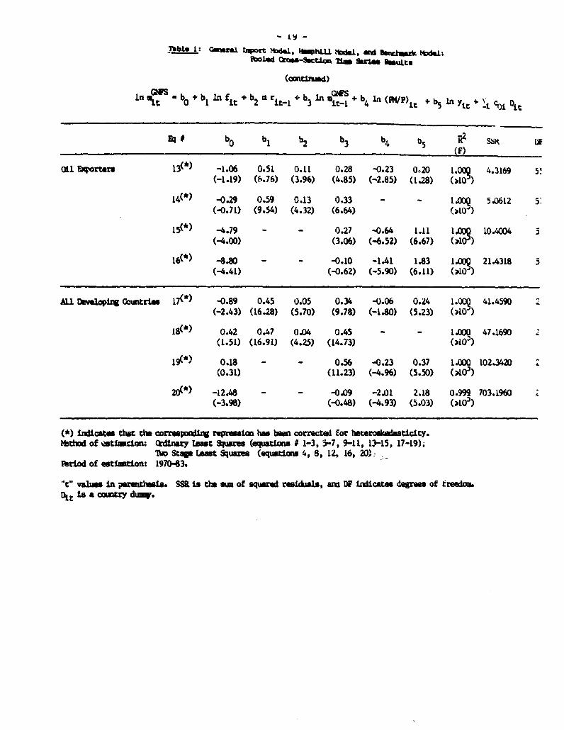
Table 1: Geral lqport Mdul, HnphIl Mbd91. ard kujm nh kl:ooled Cros-saction Tl$ Uri" mulatc

in mitf - bo I b in f it + b2 m rit_l + b3iln mit-I + b$ In (FEWP)it + b 5 In Yit +J c( Dlt

Eq# b2 b3 b4 b5 ssa or

LOW owlo Comntrne 1 -0.64 0.62 0.05 0.25 -0.03 0.17 0.992 0.3617 55(-0.93) (8.21) (2.24) (3.43) (-0.43) (1.63) (891.4)

2 0.13 0.68 0.03 0.29 - - 0.992 0.3877 57(0.27) (9.71) (1.37) (4.01) (1107.6)

3 0.52 - - 0.66 -0.08 0.24 0.976 1.1421 57(0.45) (5.96) (-0.78) (1.58) (370.6)

4 -3.25 - - 0.49 -0.64 0.86 0.962 1.7957 57(-1.05) (2.62) (-1.50) (1.75) (234.2)

tior bo?tr ollbat acturs 5(*) 0.00 0.31 0.08 0.39 -0.08 0.21 1.0O 11.272) 67

(0.00) (7.73) (4.52) (6.05) (-1.44) (3.02) (10')

6(*) 1.07 0.52 0.31 0.07 - - 14XQ 13.0094 69(2.01) (9.70) (7.i4) (3.97) (10 )

7(*) 0.62 - - 0.63 -0.22 0.27 14Xo9 28.8034 69(0.60) (6.62) (^2.61) (2.47) (>10')

8(*) -9.88 - - 0.44 -1.41 1.39 1.00l 115.6520 69(-2.06) (2.12) (-2.72) (2.73) 110 )

Non Fuel Pdim ry0oaod± ty Eporters 9 -1.00 0.47 0.04 0.31 -0.06 0.28 0.961 0.3176 55

(-1.76) (8.58) (2.44) (3.97) (-1.14) (2.34) (177.3)

10 -0.01 0.53 0.03 0.46 - - 0.959 0.3493 - 57(-0.03) (10.31) (2.03) (8.82) (214.1)

11 -1.18 - - 0.39 -0.22 0.68 0.893 0.9069 57(-1.25) (3.07) (-2.63) (3.79) (77.4)

12 -7.81 - - -0.52 -1.76 2.33 0.538 6.4982 57(-2.00) (-0.98) (-2.42) (2.64) (11.6)

- ly -

Thblej: _Is ntl C bdl.., IhtL Mada * al d U1eA1uk tD1:Pto1d _9gg-~CC±a. U hrias Uult.

(axltiud)

'it ° b 2 Ib it 2s e b3 ln *it-i 4 'A (FM/P) b

&i 1 bo bI b2 b3 b4 b5 SSK L*(F)

oil Exportrs 13(0) -1.06 0.51 0.11 0.28 -0.23 020 1.00 4.3169 5-(-1.19) (4.76) (3.96) (4.85) (-2.85) (1.28) (010 )

14(*) -0.29 0.59 0.13 0.33 _ 1O 5.0612 5(-0.71) (9.54) (4.32) (6.64) (010 )

15(*) -4.79 - _ 0.27 -0.64 1.11 1.00Q 10.4004 3(-4.00) (3.06) (-6.52) (6.67) ,10-)

16(*) -8.80 - - -0.10 -14 1.83 1.W0 21.4318 5(-4.41) (-0.62) (-5.90) (6.11) (>1O )

AUX D m loping Cmtmrie 17(*) -0.89 0.45 0.05 0.34 -0.06 0.24 1.O 41.4590 2(-2.43) (16.28) (5.70) (9.78) (-1.80) (5.23) (A0 )

18(*) 0.42 0.47 0.04 0.45 - - 1.000 47.1690 2(1.51) (16.91) (4.25) (14.73) (p.o,)

19(*) 0.18 - - 0.56 -0.23 0.37 1.000 102.342D 2(0.31) (11.23) (-4.96) (5.50) (Al0')

200*) -12.48 - - -0.09 -2.01 2.18 0.999 703.1960 2(-3.98) (-0.48) (-4.93) (5.03) (,G')

n*) i cKlcs ttat tha cormpoKifrE repesin hs bow comrcteA for heteronkadasticity.thod of esticLzuon Odinary leat Squs (equations # 1-3, 3-7, 9-11, 1-15, 17-19),

I1 Ste tEt Squae (equationw 4, 8, l2, 16, 20)<;Period of estlzmtoa: 1970-83.

"t" values In parenth; is. SSR is tlh sun of squared residuals, ant DP indicatas degree of freedLt a a country du.

- 20 -

only three out of five cases (with one estimate being significant at the

one percent level., and the other two at the 5 and 10 percent level,

respectively). Long run elasticities are somewhat higher in absolute

value: income elasticities range between 0.2 and 0.4, and price

elasticities range between -0.3 and -0.1.

The equations following the results for the general model

(equations 2 and 3 for low-income countries) present the estimates for the

two special cases, the Hemphill and benchmark models. These results again

seem to £ it th� data quite well; all the coefficients have the expected

signs and they are usually statistically significant (at the one percent

level). Estimates of the foreign exchange and reserve elasticities (b1 and

b2) in the Hemphill model oscillate around 0.5-0.6 and 0.1, respectively.

They are generally higher than the corresponding elasticities in the

general import model, but not by much. For example, estimates of b1 and

are 0.59 and 0.13 for oil exporters in the Hemphill model, compared with

estimates of 0.51 and 0.11 in the general model. By contrast, price and

income elasticities (b4 and b5) in the benchmark model are generally much

higher than the corresponding elasticities in the general import model.

For example, estimates of b4 and b5 are -0.64 and 1.11 for oil exporters in

the benchmark model, compared to estimates of -0.23 and 0.20 in the general

model. The differences in the estimated coefficients in the Hemphill and

benchmark models, when compared to the corresponding parameters in the

general import model, are due to the omission of relevant variables in the

former models -- and the magnitude of this difference suggests the extent

of the bias.

To compare explicitly the explanatory power of the general model

with the two special cases, I used tho conventional "" test. This

- 21 -

comparison shows that the general model dominates the benchmark model

quite strongly -- in all cases. It also dominates the Hemphill model in

two of the four country groups considered here (oil exporters and major

exporters of manufactures), as well as in the estimates for all

developing countries. 13/ The conclusion is that the general model

should be preferred to either the Hemphill or the benchmark model. As a

consequence, import equations that do not incorporate variables

capturing the stringency of foreign exchange constraints (ft, rt_,), or

relative prices and income (PMt/Pt, yt) are likely to produce biased

estimates due to the omission of relevant variables. The main concern

with these results, however, is that they implicitly assume that the

real import price is exogenous. 0

The second general model presented here is formed by equations

(9a) and (4). It assumes that import volumes and import prices are both

endogenous. Since import prices do not appear explicitly in equation

(9a), consistent estimates of this equation can be obtained by Ordinary

Least Squares. These estimates are shown in equations 2, 6, 10, 14 and

18 in table 1 and were already disceussed. The OLS estimates of the

import demand equation (4) are, however, biased and inconsistent -- if

(PM/P)t is indeed endogenous. In this case, consistent estimates of the

import demand equation can be obtained through the use of an

Instrumental Variable estimator, such as Two-S age Least Squares

(2SLS). These estimates are presented in the last set of regressions

for each country group (in equations 4, 8, 12, 16, and 20) in table 1.

13/ The corresponding "F" values are reported in Moran (1987), Table A-4.

- 22 -

Observe again that the price and income elasticities oE import dematid

changed significantly, when compared with the OLS estimates (and they

are also very different from the corresponding estimates in equation

(11)). For example, the new estimate of the price elasticity for oil

exporters is -1.41, compared with a previous estimate of -0.644 These

results suggest that the OLS bias in the price elasticity of import

demand may indeed be substantial.

A formal Wu-Hausman test was u.ed to test for the implicit

bias in the OLS estimate of the price elasticity of import demand (a, in

equation (4)). The results of this test suggest that the bias in the

estimate of a1 is substantial, except for low-income countries. The

conclusion is that, under a more flexible interpretation of the import

model which allows for endogenous prices (and an explicit role for

foreign exchange receipts), the traditional price and income elasticity

estimates of import demand obtained by OLS are likely to be subject to

significant biases.

4. Summary and Conclusions

Two main import models were developed. The first model

introduced two sets of explanatory variables: relative prices and

domestic output; and foreign exchange receipts and irternational

reserves. The reduced form estimates obtained from this model produced

long-run foreign exchange elasticities that ranged between 0.5 and 0.8,

reserve elasticities that oscillated around 0.1, price elasticities that

ranged between -0.3 and -0.1, and income elasticities that ranged

between 0.2 and 0.4 (table 2). This general import model contains as

special cases the models normally &dopted in the estimation of import

- 23 -

equations -- the benchmark and Hemphill models. A simple P test was

then used to determine whether this general model dominated each of the

two submodels. The results suggest that this is generally the case.

The general model dominates strongly the benchmark model in all cases.

It also dominates the Hemphill model in two of the four country groups

considered and in the estimates for all developing countries. Thus, the

elasticities obtained from either of the two submodels are likely to be

biased due to the omission of relevant variables. The main concern with

these results, however, is that the real import price is assumed to be

exogenous in the estimation of these models.

The second import model developed here assumes that import

volumes and import prices are both endogenous, and allows explicit

testing of the latter assumption. This second model includes two

independent structural equations: an infinitel,. inelastic import-supply

curve, and a normal downward-sloping demand curve. Two implications of

this model were noted. First, since the supply curve is infinitely

inelastic and does not respond to changes in domestic output, import

volumes depend only on foreign exchange receipts and international

reserves -- an implication that can certainly be relaxed (see section

5). Second, the import demand curve, which serves to determine the

appropiate real import price, cannot be estimated by Ordinary Least

Squares since this will produce biased and inconsistent estimates of its

parameters. To test for the implicit bias in the OLS estimates (or, for

the endogeneity of the real import price), the Wu-Hausman test was

performed -- rhe test compares these estimates with those obtained with

- *t -

hbbJ 2: 1mW-SAn Z.Wt gLmtuAclt.: pfoj a g.geSkt Ss- bmi Auta

bftii i F*m tlc±tli Elo Cicitls Of 1iWort DId(~mrai !swst IWIdth _am Prlme) a OLS bttem b/ -s t

eeLtLt tT ¢T I? T LLT LT

t1w Dv= C1 m rim 0.83 0.07 -0.04 0.23 -0.24 0.71 -1.26 1.69

MaJor awtmnof .bzuactwe 0.51 0.13 -0.13 0.34 -0.59 0.73 -2.52 2.48

~nRai fr1MUOdity bpor 0.68 0.06 -0.09 0.41 -0.36 1.11 -1.76 2.33

O(l Exprtmrm 0.71 0.15 -0.32 0.28 -0.87 1.52 -1.41 1.83

AU DNwl1CP.mEtri± 0.68 0.06 -0.09 0.36 -0.52 0.84 -2.01 2.18

*/ In lag tm eLti_i mm calogate a bi/(1-b 3 ), or, a aj/(1_-3), for I - f, r, y, p; e=spt as zto&

/1 elasticities w obtained frmo the Smmai Dort modl (.qumct (11)) mtias by as.

b/ hmm elmticitsm mor obtaiA from ttn bxnuk 1l (mquatlcn (4)) mtc1te by OL.

C lhmse alticities mrs obtald from the b_Klumikti (equtiAo (4)) estiated by 2S. 'TU long ruI prdc -in elastiritis rdoi for Nn-?uml ftliry tdity Eport, Ol1 iAportmrs, a AU LNalopiM amtrfO:XrsSIIW~ to the atlatas of &I, and a2 resPctively (sin=e a3 wm not statistically slfcmnit at c.wc'misliifiomxa lews).

- 25 -

a consistent procedure, such as Two-Stage Least Squares. This test

showed that the OLS estimates of the import demand curve are subject to

significant biases, a result that again confirms the importance of

foreign exchange constraints in the analysis of import behavior in

LDCs. The long-run price and income elasticity estimates of import

demand for each of four country groups, using OLS and 2SLS, are reported

in the last four columns of Table 2. In all cases, the 2SLS estimates

-- which use foreign exchange receipts and international reserves as

instruments -- are much higher in absolute value than the corresponding

estimates obtained with OLS.

In sum, the main conclusion obtained from the present study is

that, while price and income effects are important in the analysis of

import behavior in developing countries, foreign exchange constraints

also play a critical role in determining imports -- as they strongly

affect import volumes. Hence, import models that neglect either of

these effects will yield biased estimates for developing country

imports.

An important implication of this result is that policies

concentrating exclusively on aggregate demand (fiscal and monetary

policies) or on switching expenditures between tradables and

nontradables (exchange rate policies) will have a limited effect on

import volumes - although they will certainly affect import demand. By

contrast, policies that directly affect export earnings and capital

inflows will likely yield a more drastic response in import volumes in

LDCs. Although policies designed to affect the latter variables

generally entail a significant domestic adjustment effort in the

developing countries, their success -- in maintaining a smooth flow of

- 26 -

imports -- will also depend on the continued access of LDC exports to

industrial country marketo, and on increased access to external capital

flows, both from official and private sources.

5. Areas of Future Research

This paper has provided a stylized model of import behavior for

developing countries. Actual policymaking may require, however, a more

careful look at some of the key assumptions underlying this approach. I

briefly mention three areas that would enrich the analysis and that may

have a significant effect on the results discussed here. The first area

concerns the simplicity of the dynamic structure imposed on the modelb

presented in this study. The second area concerns the economic

interpretation of both the Hemphill and the general import models. The

third area concerns the exogeneity assumption of foreign exchange

receipts and domestic output in the implementation of these models.

Consider first the dynamic structure. Only one lagged

dependent variable was introduced here to capture adjustment costs: that

is, to capture the costs of changes in the level of imports from one

period to the next, due to changes in the exogenous variables. 14/ The

implicit dynamic structure of this model -- known in the literature as

the "partial adjustment" model -- has been cr'-icized as being naive and

sometimes misleading. Instead, Hendry and others (1986) have proposed

the use of a general dynamic structure, which in the Hemphill model can

be written in the following way:

14/ Hemphill also considers one lagged value of foreign exchangereceipts, but the coefficient associated with this variable did notprove significant in this study.

- 27 -

*(W)t '- 91 ft + 02 (L)rt_i et

where *(L), e1(L) and a2(Lt are polynomials in the lag operator L,

and et is a random noise process. To facilitate its implementation,

they have proposed a set of tests to obtain a parsimonious

representation (see Hendry and others 1986, for the details of this

procedure). Only then could the dynamics be fully captured, and the

resulting equation used for predictive purposes.

To see how this general dynamic structure can arise naturally

in import models discussed here, consider again the simple Hemphill

model, equation (9):

(1-b3L) t= b0 + 1 ft + b2 L rt (9)

If foreign exchange receipts (ft) are decomposed into its two main

components -- export receipts and net capital inflows -- and a simple

linear behavioral equation is introduced for the latter variable, this

gives:

f * .P +k(xP, t k 60 + +1 + t 2Yt 3 t (9.1)

where 61 2 0, 42 2 O, 63 0, and

tP =* nominal exports deflated by the import price (or

purchasing power of exports)$

xtP (y -) long run or expected value of x p (y );t tt t

- 28 -

Z - vector of other exogenous variables which are relevant

for the determination of real net capital inflows (such

as external economic activity, a proper set of domestic

and foreign real interest rates, and the country's

initial debt service ratio).

Assume, for simplicity, that expectations about z p and Yt are formed

adaptively, so that:

zP* )Lj p yt xI t Yt ' p 2/(1-( -A2)LI t

with 0 S A1' A2 S 1.

Substituting these two expressions into equation (9.1), and the

resulting expression into equation (9), gives:

t(L) m O =b0 + 1 (L) x + e 2 (L) y + 3 (L) Zx + 4 (L) r

where,

*(LW (1-b3 L) (1-(l-X 1) L) (1-(l-X 2) L)

el(L) bi (l-(l-x ) L) (1-(l-X2) L) + b 1 A1 61 (-(I2 2 L

e2(L) b1 A2 62 (l-(l-x1) L)

e3(L) - b1 a3 (1-(l-xl) L) (1-(1- k2) L)

e 4(L) b2 (l-(l-A I) L) (1 (1- A2)L)

In this version of the model, export receipts (x p), aggregate outputt

ytpinternational reserves (rt_.i), and other exogenous variables

- 29 -

(relevant to the determination of net capital inflows) all play an

independent role in determining imports, and the dynamic structure

imposed on the model is indeed quite rich.

Consider now the economic rationale behind the optimization

function used by Hemphill (presented in equation 5) and its

generalization (equation 5'). Despite their obvious intuitive appeal --

discussed in section 2 -- these optimization functions are somewhat ad

hoc. An alternative scheme with a clear economic rationale has been

developed by Sachs (1981 and 1982) and Dornbusch (1983). In these

studies, imports are derived from an intertemiiral utility maximization

problem, where expectations of future events and wealth play prominent

roles. This scheme is clearly more appealing from a theoretical

standpoint than the approach adopted here, but it is difficult to

implement empirically.

Winters (1987) developed two empirical versions of these models

(which he labeled "equilibrium" and "disequilibrium" versions) and found

that the results, although promising, are not without problems, and that

the empirical estimates do not appear much better than other simpler

alternatives -- like the Hemphill model. More important, however, is

that the intertemporal models developed by Sachs and Dornbusch assume

perfect capital markets (the country can borrow unlimited amounts at a

constant interest rate), an assumption that may not be appropriate for

most developing countries, particularly in the 1980s. Thus, while

Winters' results clearly vindicate the simple Hemphill model -- and its

generalization, the general import model developed here -- there is

obviously scope for improvement in the theoretical analysis of these

models.

-30-

Finally, consider the exogeneity assumption about foreign

exchange receipts, ft, and total value added, Yt, In section 2 I argued

that ft can reasonably be assumed to be exogenous to the current import

decision. This presumes, in particular, that external borrowing car be

decomposed into an autonomous (exogenous) and an accomodating

(endogenous) component. Hemphill (1974) and Winters and Yu (1985) have

discussed the difficulties of this distinction. The problem may be

complicated further. For example, a sudden shortfall in imports -- due

to a cutback in foreign lending -- may have an effect on exports or on

total value added (GDP) in the same period, as essential imported inputs

are curtailed. Reserves can be used to cut this contemporaneous link,

but this possibility is available only for a limited time. In short,

the exogeneity of ft and yt should be tested rather than assumed, using

tests such as those proposed by Granger and Sims (see Geweke 1986 for a

recent survey of this literature). If these tests show any sign of

feedback, a more general model -- where ft, yt, and mt are

simultaneously determined -- will have to be developed. This general

model could then be estimated simultaneously, or the appropriate reduced

form for imports derived and then estimated.

- 31 -

REFERENCES

Anderson, T.W., and C. Hsiao. Formulation and Estirmation of Dyr.amic

Models Using Panel Data, Journal of Econometrics, 18 (1982), pp.

47-82.

Chu, K., E. C. Hwas and K. Krishnamurty. Export Instability and

Adjustment of Imports, Capital Inflows, and External Reserves: A

Short Run Dynamic Model, in D. Bigman and T. Taya (eds.), Exchange

Rate and Trade Instability, Ballinger (1983).

Dornbusch, R. Real Interest Rates, Home Goods and Optimal External

Borrowing, Journal of Political Economy, 11(1983), pp. 141-153.

Ceweke, J. Inference and Causality in Economic Time Series Models, in Z.

Griliches and M.D. Intriligator (eds.), Handbook of Econometrics,

vol. II, Elsevier Science Pub. (1986), ch. 1S.

Goldstein, M., and M. Khan. Income and Price Effects in Foreign Trade,

in R.W. Jones and P. B. Kenen (eds.), Handbook of International

Economics, vol. II, Elsevier Science Publishers (1985).

Hemphill, W. The Effect of Foreign Exchange Receipts on Imports of Less

Developed Countries, IMF Staff Papers, 21(1974), pp. 637-677.

Hendry, D., A.R. Pagan, and J.D. Sargan. Dynamic Speicfication, in Z.

Griliches and M.D. Intriligator (eds.), Handbook of Econometrics,

vol. III, Elsevier Science Pub. (1986(, ch. 18.

Khan, M. Import and Export Demand in Developing Countries, IMF Staff

Papers, 21(1974), pp. 678-693.

Khan, M., and K. Ross. The Functional Form of the Aggregate Import

Equatiou, Journal of International Economics, 7(1977), pp. 149-160.

Magee, S. Prices, Income and Foreign Trade: A Survey of Recent Economic

Studies, in P. Kenen (ed.) International Trade and Finance:

Frontiers for Research, Cambridge University Press (1975), pp. 175-

252.

Mirakhor, A., and P. Montiel. Import Intensity of Output Growth in

Developing Countries, 1970-85, in IMF, World Economic Outlook

(April 1987).

Moran, C. Import Behavior in Developing Countries, Trade Policy

Division (CEC), World Bank (November 1987).

Nickell, S. Biases in Dynamic Models with Fixed Effects, Econometrica,

49 (1981), pp. 1417-1426.

- 32 -

Sachs, J. The Current Account and Macroeconomic Adjustment in the1970's, Brookings Papers in Economic Activity, 10(1981), pp. 201-68.

Sachs, J. The Current Account in the Macroeconomic Adjustment Process,Scandinavian Journal of Economics, 84(1982), pp. 147-59.

Sundararajan, V. Exchange Rate Versus Credit Policy, Journal ofDevelopment Economics, 20(1986), pp. 75-105.

m i3an, W.N. Endogeneity Testing in a Supply and Demand Framework,Review of Economics and Statistics, 68 (1986), pp. 638-46.

Thursby, J., and M. Thursby. How Reliable Are Simple, Single EquationSpecifications of Import Demand?, Review of Economics andStatistics, 66(1984), pp. 120-28.

Winters, L.A. An Empirical Intertemporal Model of Developing Countries'lu3orts, Weltwirtschaftliches Archiv, 123 (1987), pp. 58-80.

Winters L. A. and K. Yu, Import Equations for Global Projections, mimeo,Clobal Analysis and Projections Division (EPD), World Bank (May1985).

World Bank. World Development Report 1986, Oxford University Press(1986).

- 33 -

APPENDIXThe Data

The data in this study can be defined formally as follows:

mGNPS , Imports of goods and nonfactor services in constant

dollars, obtained from the World Bank's Balance of

Payments database, deflated by PMt. 1/

PMt - Merchandise import deflator in U.S.$, calculated by

the World Bank (based on disaggregated import data

at the country level). 2/

Pt - DP deflator in U.S.$, obtained from World Bank's

National Accounts database.

'it - CDP at market prices in constant dollars, obtained

from the World Bank's National Accounts database.

rt a End-year stock of international reserves, obtained

from the World Bank's Balance of Payments database,

deflated by PMt.

ft a Foreign exchange receipts = exports of goods and

nonfactor services + net factor income + net

transfers + capital inflows (including direct

1/ Note that there is no deflator for imports of GNFS at the countrylevel derived with a comparable methodology (the implicitnational accounts deflator will not be appropriate for thispurpose). This explains why I used PMt as the appropriatedeflator.

2/ See C. Moran and J. C. Park, Merchandise Trade Deflators forDeveloping Countries, World Bank, EPD, Division Working Paper No.1986-7 (June 1986) for a discussion of the method used to obtainthe trade deflators.

- 34 -

private investment, long and short term loans, plus

errors and omissions), obtained from the World

Bank's Balance of Payments database, deflated by

PMte 3/

2. Country Classification: The countries chosen in this

study were taken to be representative of each of the main groups

distinguished in the World Bank's 1986 World Development Report:

i) Low Income Countries: India, Pakistan, Kenya, Sudan and

Senegal.

ii) Major Exporters of Xanufactures: Korea, Argentina,

Brazil, Portugal, Thailand and Yugoslavia.

iii) Non-Fuel Primary Commodity Exporters t- Other Oil

Importers): Colombia, Chile, Morocco, Turkey, Cote

D'Ivoire.

iv) Oil Exporters: MeAico, Indonesia, Nigeria, Peru and

Algeria.

3/ I also used a narrower definition of foreign exchange receiptswhich excluded short-term borrowing. The results obtained withthe broader definition, however, were consistently better.

Title Author Date

WPS1 Imports Under a Foreign Exchange Cristian Moran March 1988Constraint

WPS2 Issues in Adjustment Lending Vinod Thomas March 1988

WPS3 CGE Models for the Analysis of TradePolicy in Developing Countriesin Developing Countries Jaime de Melo March 1988

For information about obtaining copies of papers, contact the ResearchAdministrator's Office, 473-1022.