Implied Volatility, Fundamental solutions, asymptotic ... · Implied Volatility, Fundamental...
57
Implied Volatility, Fundamental solutions, asymptotic analysis and symmetry methods, Linz, Ricam kick-off Workshop, September 11, 2008 Peter Laurence Dipartimento di Matematica e Facolt ´ a di Statistica, Uni. Roma 1 Implied Volatility, Fundamental solutions, asymptotic analysis and symmetry methods, Linz, Ricam kick-off Workshop,September 11, 2008 – p. 1/4
Transcript of Implied Volatility, Fundamental solutions, asymptotic ... · Implied Volatility, Fundamental...
Implied Volatility, Fundamental solutions,asymptotic analysis and symmetry
methods,
Linz, Ricam kick-off Workshop,September 11, 2008
Peter Laurence
Dipartimento di Matematica e Facolta di Statistica, Uni. Roma 1
Implied Volatility, Fundamental solutions, asymptotic analysis and symmetry methods, Linz, Ricam kick-off Workshop,September 11, 2008 – p. 1/47

Main aims of this contribution
Outline of talkRapid review Implied Volatility, local volatility, mimicking behaviour. Practitioners like closedform formulas for calibration.
Review Heat Kernel approach to solving stochastic volatility models. Hagan-Lesniewski,Henry-Labordère.
Refined asymptotics for a class of generalized SABR like models. Joint work with GérardBen Arous and Tai-Ho Wang. Influence of curvature.
Interaction between symmetry and heat kernel approach. Distance function: Work inprogress with Matveev and Wang.
Implied Volatility, Fundamental solutions, asymptotic analysis and symmetry methods, Linz, Ricam kick-off Workshop,September 11, 2008 – p. 2/47

Quick Overview 1
The goal, from PDE point of view, is to solve parabolic equations in one or several spatialdimensions.
On [0, T ], where T is the maturity of European option, solve:
ut + aij(x)uxixj + biuxi − ru = 0,x ∈ Ω ⊂ Rn, t ∈ [0, T ]
u(x, T ) = ψ(x) final condition
The matrix aij is usually degenerate, so the operator above is often not uniformlyparabolic.
Researchers in PDE are used to seeing the equation expressed as initial value (rather than finalvalue) problem. This can be achieved, by making the change of variables: τ = T − t. The problemthen reads as:
uτ − aij(x)uxixj − biuxi + ru = 0,x ∈ Ω ⊂ Rn, t ∈ [0, T ]
u(x, 0) = ψ(x) initial condition
Implied Volatility, Fundamental solutions, asymptotic analysis and symmetry methods, Linz, Ricam kick-off Workshop,September 11, 2008 – p. 3/47

Fundamental solution
We are interested in finding a fundamental solution of such parabolic equations:
F (x, t, ξ, T ),x, ξ ∈ Ω, t ∈ [0, T ]
Often Ω is Rn or R
n+.
Here F satisfies the parabolic equation in the variables x and t and has a delta function finalcondition:
F (x, T, ξ, T ) = δξ(x)
• We may wish to add additional boundary conditions, such as in the case of the valuation ofbarrier options, and in this case, we seek the Green’s function, rather than the Fundamentalsolution. . In the context of heat kernels we are then led to consider the Dirichlet heat kernel andthe Neumann heat kernel.• Degeneracy : In mathematical finance, additional subtleties arise due to the degeneracy of theprincipal part at the boundary (Stochastic CEV models) or in the entire domain (Asian Options).
Implied Volatility, Fundamental solutions, asymptotic analysis and symmetry methods, Linz, Ricam kick-off Workshop,September 11, 2008 – p. 4/47

Finance in the News
Quote from article by Mike Giles and Ronnie Sircar in Siam NEWS, October 2007:
“ The major challenges in computational finance arise not from difficult geometries, as inmany physical problems, but from the need for rapid calculation of an EXPECTATION or thesolution of its associated Kolmogorov partial differential equation.”
“ Efficiency is at the forefront, because models are re-estimated as new market data arrivesand calibration (or “marking to market”) embeds the expectation/PDE calculation in aniterative solution to an inverse problem”’
Interpretation of last sentence: from traded market prices back out parameters incoefficients of parabolic operator and/or back out the functional form of these coefficients.
Implied Volatility, Fundamental solutions, asymptotic analysis and symmetry methods, Linz, Ricam kick-off Workshop,September 11, 2008 – p. 5/47
Closed Form or quasi-closed form solutions: A Mathematician’s Toolbox
Recent years have seen surge in attempts to find closed form or quasi-closed form solutions tocertain parabolic problems arising in option pricing. In today’s talk, we will concentrate on one of
these, asymptotics. The other approach, which we will not discuss in detail, for lack oftime,is:
1)Changes of Variables, Transformation Groups and Lie Symmetry Analysis.Literature (Partial List):
Albanese and Kusnetsov: Reducing time homogeneous one dimensional diffusions tostandard form and solving via special functions.Transformations of Markov Processes and Classification Scheme for Solvable DriftlessDiffusions. Preprint 2005
Carr, Laurence and Wang: Reducing time inhomogeneous diffusions to standard form. Via Liesymmetry considerations. Comptes Rendus de l’Académie des Sciences, 2006.
Linetsky: Time homogeneous one dimensional diffusions. Approach via eigenfunctionexpansions. Int. J. Theor. Appl. Finance 7 (2004).
Ait-Sahalia: Annals of Statistics, 2007 “Closed-Form Likelihood Expansions for MultivariateDiffusions”. Reduction method to heat equation with lower order terms.(related to Lie).
Implied Volatility, Fundamental solutions, asymptotic analysis and symmetry methods, Linz, Ricam kick-off Workshop,September 11, 2008 – p. 6/47
Sabr Models and generalized SABR models
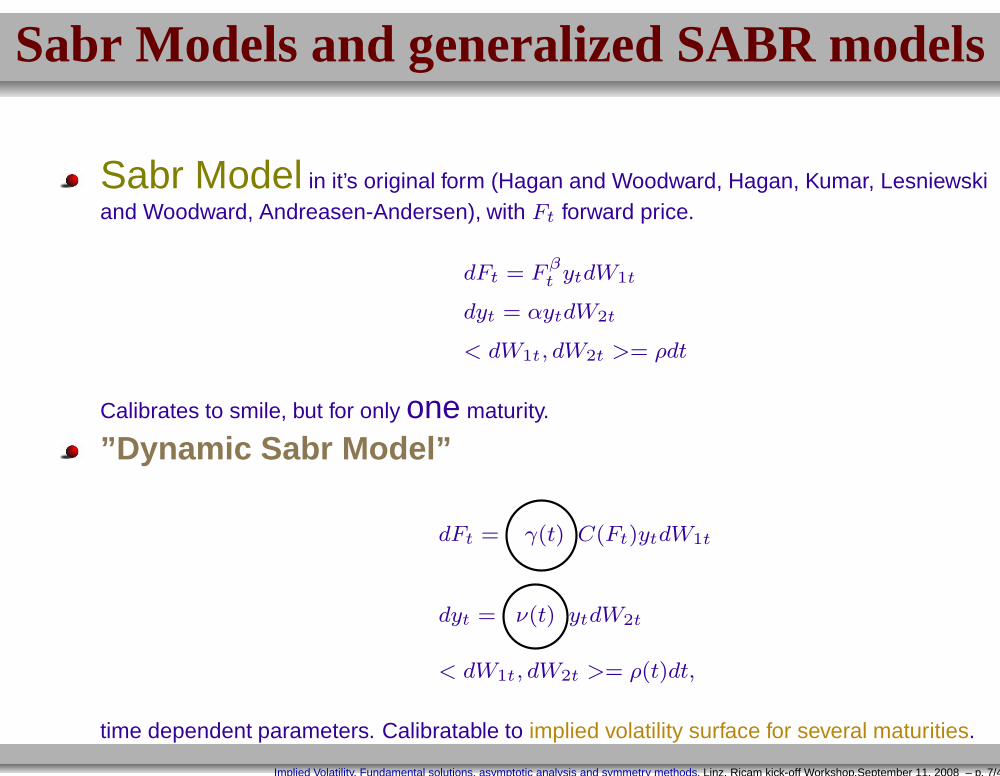
Sabr Model in it’s original form (Hagan and Woodward, Hagan, Kumar, Lesniewskiand Woodward, Andreasen-Andersen), with Ft forward price.
dFt = Fβt ytdW1t
dyt = αytdW2t
< dW1t, dW2t >= ρdt
Calibrates to smile, but for only one maturity.
”Dynamic Sabr Model”
dFt = γ(t) C(Ft)ytdW1t
dyt = ν(t) ytdW2t
< dW1t, dW2t >= ρ(t)dt,
time dependent parameters. Calibratable to implied volatility surface for several maturities.
Implied Volatility, Fundamental solutions, asymptotic analysis and symmetry methods, Linz, Ricam kick-off Workshop,September 11, 2008 – p. 7/47

Mean Reverting Sabr models
λ-Sabr model (incorporating mean reversion
dFt = νC(Ft)ytdW1t
dyt = κ(θ − yt)dt+ γytdW2t
< dW1t, dW2t >= ρdt
Introduced by Henry-Labordère (2005).
dFt = C(Ft)yδt dW1t
dyt = κ(θ − yt)dt+ yδt dW2t
< dW1t, dW2t >= ρdt
The homogeneous "delta-geometry" introduced by Bourgade and Croissant(2005).
Implied Volatility, Fundamental solutions, asymptotic analysis and symmetry methods, Linz, Ricam kick-off Workshop,September 11, 2008 – p. 8/47

Generalized Sabr models
dFt = γ(t)C(Ft)yδt dW1t
dyt = κ(θ − yt)dt+ w(yt) dW2t
< dW1t, dW2t >= ρdt
Generalized class of SABR models introduced by G. Ben Arous, P. Laurence, TH Wang(2008): Try to understand how the asymptotics depends on function w(y). Also, refine andgeneralize existing asymptotics.
Osajima (2007): Approach to SABR models using Malliavin calculus. Easily quantifiableresults only for original (lognormal) SABR models.
Implied Volatility, Fundamental solutions, asymptotic analysis and symmetry methods, Linz, Ricam kick-off Workshop,September 11, 2008 – p. 9/47
Approaches to the asymptotic expansions, I
Three (loosely speaking) different approaches:
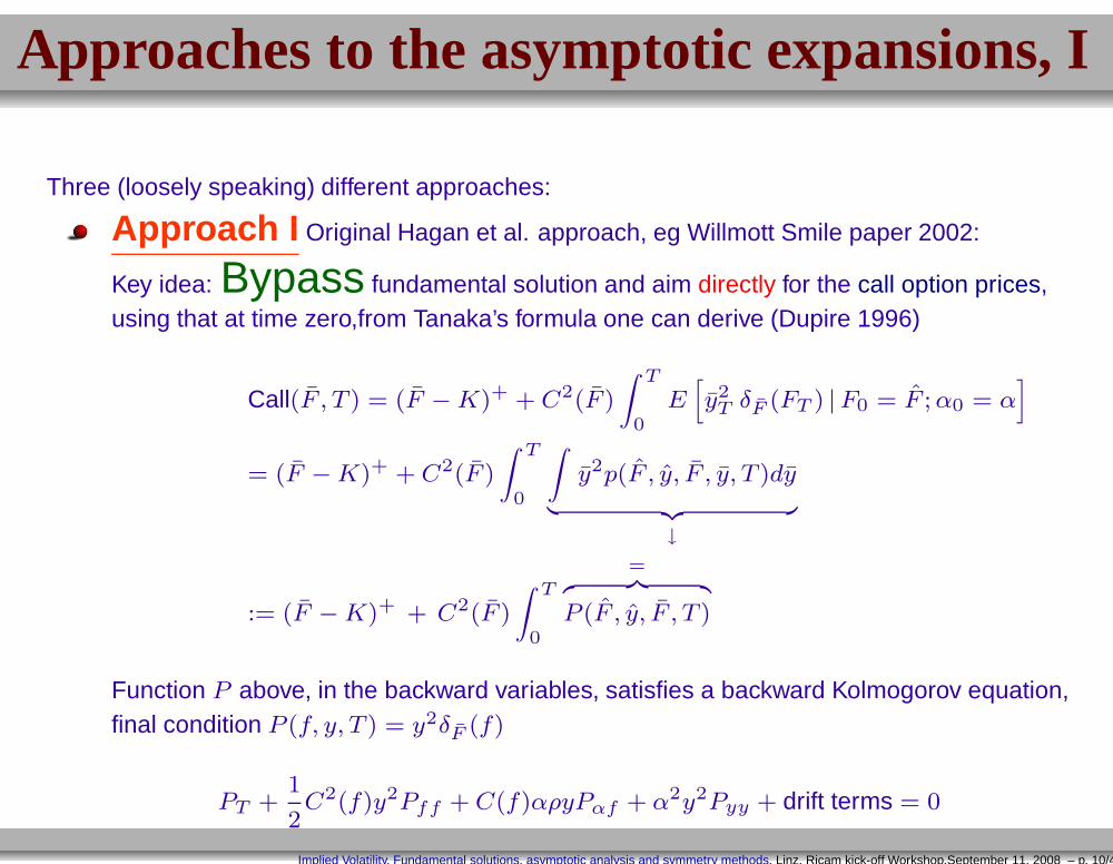
Approach I Original Hagan et al. approach, eg Willmott Smile paper 2002:
Key idea: Bypass fundamental solution and aim directly for the call option prices,using that at time zero,from Tanaka’s formula one can derive (Dupire 1996)
Call(F , T ) = (F −K)+ + C2(F )
∫ T
0E
[
y2T δF (FT ) |F0 = F ;α0 = α]
= (F −K)+ + C2(F )
∫ T
0
∫
y2p(F , y, F , y, T )dy
︸ ︷︷ ︸
↓
:= (F −K)+ + C2(F )
∫ T
0
=︷ ︸︸ ︷
P (F , y, F , T )
Function P above, in the backward variables, satisfies a backward Kolmogorov equation,final condition P (f, y, T ) = y2δF (f)
PT +1
2C2(f)y2Pff + C(f)αρyPαf + α2y2Pyy + drift terms = 0
subject to the final condition P (f, y, T ) = y2δK(f) delta function one variable.Implied Volatility, Fundamental solutions, asymptotic analysis and symmetry methods, Linz, Ricam kick-off Workshop,September 11, 2008 – p. 10/47

Approaches to the asymptotic expansions, II & III
Approach II Geometric ApproachGeometric/Analytic approachThis approach was introduced by Lesniewski in a lecture at the Courant Institute. Uses thehyperbolic plane. Generalized by several papers: Introduction of McKean heat kernel (seepage 50), ie. fundamental solution of heat equation in hyperbolic plane, plays a central role.
Henry-Labordere (2005) introduces the use of the heat kernel expansion and the λ Sabrmodel
Geometric/Stochastic approach Ground breaking work by Varadhan (1965) and then byMolchanov (1975)and Azencott (1981), Ben Arous (1989). This is followed by the work byBourgade and Croissant (2005) who apply Molchanov’ s results to stochastic volatilitymodels.
Approach III Malliavin stochastic calculus of variations based approach, based onwork of Bismut, Kusuoka, Malliavin, due to Takahashi (1999-2008) at al.(also Fournier-Lionset al. for calculation of Greeks) and, more recently, by Osajima (2007, 2008), based on workof Kusuoka.• Also, Fouque, Papanicolaou, Sircar fast mean reverting SV models, and Alan LewisFourier Transform based methods.
Implied Volatility, Fundamental solutions, asymptotic analysis and symmetry methods, Linz, Ricam kick-off Workshop,September 11, 2008 – p. 11/47

Preliminaries on implied and other volatilities
Local volatility models: dSt = Stσ(St, t)dt+ rSdt
Dupire’s formula: From traded option prices to parametric form of σ(F, t).
σ2loc(S, t,K, T ) =
∂C∂T
+ rK ∂C∂K
12K2 ∂2C
∂K2
From local volatility to implied volatility and vice-versa (fully non-linear PDE)
σ(log(
x︷︸︸︷
S
K), T ) =
2TI ∂I∂T
+ I2
(1 − x∂I∂xI
)2 + TI ∂2I∂x2 − 1
4T 2I2 ∂2I
∂x2
, (take r =0)
Approximate relationship ( Berestycki-Busca-Florent, QF 2002) as τ = T − t→ 0:
limτ→0
I(log(F
K), τ) =
1∫ 10
1
σ(s log( FK
),0)ds,
uniformly as τ → 0. Ie. Implied volatility is the harmonic mean of local volatility, in small timelimit.
Implied Volatility, Fundamental solutions, asymptotic analysis and symmetry methods, Linz, Ricam kick-off Workshop,September 11, 2008 – p. 12/47

From stochastic volatility to local volatility
Stochastic volatility models:
dFt = αtb(Ft)dW1t
dαt = g(αt)dW2t
F0 = F, α(0) = α initial conditions< dW1t, dW2t >= ρdt
Obtaining a local volatility model with same F marginals:The “equivalent” local volatility function is given by:
σ2
loc(K,T ) = b2(K)E[α2
T |FT = K]
Implied Volatility, Fundamental solutions, asymptotic analysis and symmetry methods, Linz, Ricam kick-off Workshop,September 11, 2008 – p. 13/47

Gyongi, Dupire, Atlan, Piterbarg
One can actually show a more general result Gyongi, giving rise to the concept of
"mimicking" multi-factor models with lower order ones:
dSt = c(St, νt, t)dt+ b(St, t)g(ν(t), t)dW1t
dνt = ζ(νt)dt+ β(νt)dW2tdt
< dW1t, dW2t >= ρdt
S(0) = S, ν(0) = ν,
yields the same marginal distributions with respect to the S variable as the following sde:
dSt = σ(St, t)dWt + γ(S, t)dt,
S(0) = S
where, the effective parameters are:
σ2(K,T ) = b(K,T )E[g2 |ST = K
]
γ(K,T ) = E [c |ST = K]
Implied Volatility, Fundamental solutions, asymptotic analysis and symmetry methods, Linz, Ricam kick-off Workshop,September 11, 2008 – p. 14/47
Proof (time permitting)
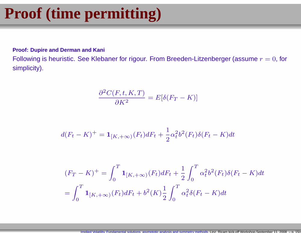
Proof: Dupire and Derman and Kani
Following is heuristic. See Klebaner for rigour. From Breeden-Litzenberger (assume r = 0, forsimplicity).
∂2C(F, t,K, T )
∂K2= E[δ(FT −K)]
d(Ft −K)+ = 1[K,+∞)(Ft)dFt +1
2α2
t b2(Ft)δ(Ft −K)dt
(FT −K)+ =
∫ T
01[K,+∞)(Ft)dFt +
1
2
∫ T
0α2
t b2(Ft)δ(Ft −K)dt
=
∫ T
01[K,+∞)(Ft)dFt + b2(K)
1
2
∫ T
0α2
t δ(Ft −K)dt
Implied Volatility, Fundamental solutions, asymptotic analysis and symmetry methods, Linz, Ricam kick-off Workshop,September 11, 2008 – p. 15/47

Proof ct’d
Taking expectations:
C(K,T ) =1
2b2(K)E
[∫ T
0α2
t δ(Ft −K)dt
]
Take the partial derivative with respect to upper limit T , get:
∂C(K, T )
∂T=
1
2b2(K)E
[α2
T &FT = K]
∂C(K, T )
∂T=
1
2b2(K)E
[α2
T |FT = K]P [FT = K]
∂C
∂T=
1
2b2(K)E
[α2
T |FT = K] ∂2C
∂K2, to conclude that
→∂C∂T
∂2C∂K2
=1
2b2(K)E
[α2
T |FT = K]
and notice that left hand side is the local volatility, using Dupire’s formula.
Implied Volatility, Fundamental solutions, asymptotic analysis and symmetry methods, Linz, Ricam kick-off Workshop,September 11, 2008 – p. 16/47

PDE view: From stochastic volatility model to local volatility
Consider a stochastic volatility model:
dFt = b(Ft)FtytdW1t, dyt = ytc(yt)dW2t, F (0) = F , y(0) = y
Recall Gyongi formula: There exist a local volatility model (ie. a model with one less state variable)
dFt = σ(Ft, t)FtdW1t
which has the same marginals with respect to the Ft process, given by
σ2(F, t) = E[b2(Ft)F
2t y
2 |Ft = F, F0 = F , y0 = y]
Let F(F , y, F, y, t) be the corresponding fundamental solution: Then in PDE language we have
(σ2)F ,y(F, T ) =F 2b2(F )
∫y2F(F , y, F, y, T )dy
∫F(F , y, F, y, T )dy
So, if we knew the Fundamental solution in closed form or in quasi-closed form, for small t, wecould recover the asymptotic value of the local volatilityand then the implied volatility, as a functionof strike K and maturity T .
Implied Volatility, Fundamental solutions, asymptotic analysis and symmetry methods, Linz, Ricam kick-off Workshop,September 11, 2008 – p. 17/47

2 approaches in analytic expansion method
Two approaches at this stage to obtaining the call option prices
In the RHS of formula:
P (F , y, t) =
∫
y2F(F , y, F, y, T )dy
insert an expansion F = F0 + tF1 + . . . valid asymptotically for small σ2T , into the aboveformula.
Approach II, mentioned earlier is to look directly for a solution of the equation satisfied by Pin the backward variables:
PT +1
2C2(F )y2PF F + C(F )αρyPyF + α2y2Pyy + drift terms = 0
subject to the final condition P (F , y, T ) = y2δK(F ) delta function one variable and, again,seek an expansion:
P = P0 + tP1 + t2P2 . . .
Implied Volatility, Fundamental solutions, asymptotic analysis and symmetry methods, Linz, Ricam kick-off Workshop,September 11, 2008 – p. 18/47
Heat Kernel Approach
Heat kernel approach ( e.g. analytical approach 1),origins are in study of small time behaviour offundamental parabolic differential equations.
Literature
Lesniewski 2001, Hagan-Lesniewski-Woodward 2004(unpublished).
Henry-Labordère, 2005. Henry-Labordère QuantitativeFinance 2007.
Implied Volatility, Fundamental solutions, asymptotic analysis and symmetry methods, Linz, Ricam kick-off Workshop,September 11, 2008 – p. 19/47
Small Time limit for parabolic problems: Where did it really begin?
• Let p(t,x,y) be the fundamental solution corresponding to the non-degenerate diffusion withinfinitesimal generator:
aij(x)pxixj , x ∈ Rn
and the time homogeneous diffusion (Heat flow) on Rn.
Hp = pt − Lxp = 0
Implied Volatility, Fundamental solutions, asymptotic analysis and symmetry methods, Linz, Ricam kick-off Workshop,September 11, 2008 – p. 20/47
Small Time limit for parabolic problems: Where did it really begin?
• Let p(t,x,y) be the fundamental solution corresponding to the non-degenerate diffusion withinfinitesimal generator:
aij(x)pxixj , x ∈ Rn
and the time homogeneous diffusion (Heat flow) on Rn.
Hp = pt − Lxp = 0
• The main theorem concerning the small time behaviour of the fundamental solution of thisequation is due to Varadhan:
limt→0
4t log(pt) = −d2(x,y),
holds uniformly for x,y in compact subsets of Rn.
Implied Volatility, Fundamental solutions, asymptotic analysis and symmetry methods, Linz, Ricam kick-off Workshop,September 11, 2008 – p. 20/47

Small Time limit for parabolic problems: Where did it really begin?
• Let p(t,x,y) be the fundamental solution corresponding to the non-degenerate diffusion withinfinitesimal generator:
aij(x)pxixj , x ∈ Rn
and the time homogeneous diffusion (Heat flow) on Rn.
Hp = pt − Lxp = 0
• The main theorem concerning the small time behaviour of the fundamental solution of thisequation is due to Varadhan:
limt→0
4t log(pt) = −d2(x,y),
holds uniformly for x,y in compact subsets of Rn.
d(x,y) is the Riemannian distance, associated to gij, inverse of aij, ds2 = gijdsidsj .
Implied Volatility, Fundamental solutions, asymptotic analysis and symmetry methods, Linz, Ricam kick-off Workshop,September 11, 2008 – p. 20/47

Riemannian distance
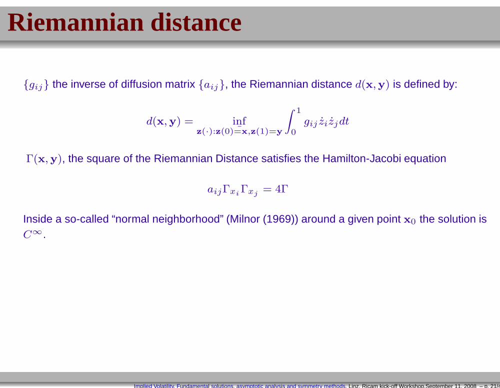
gij the inverse of diffusion matrix aij, the Riemannian distance d(x,y) is defined by:
d(x,y) = inf¯z(·):z(0)=x,z(1)=y
∫ 1
0gij zizjdt
Implied Volatility, Fundamental solutions, asymptotic analysis and symmetry methods, Linz, Ricam kick-off Workshop,September 11, 2008 – p. 21/47
Riemannian distance
gij the inverse of diffusion matrix aij, the Riemannian distance d(x,y) is defined by:
d(x,y) = inf¯z(·):z(0)=x,z(1)=y
∫ 1
0gij zizjdt
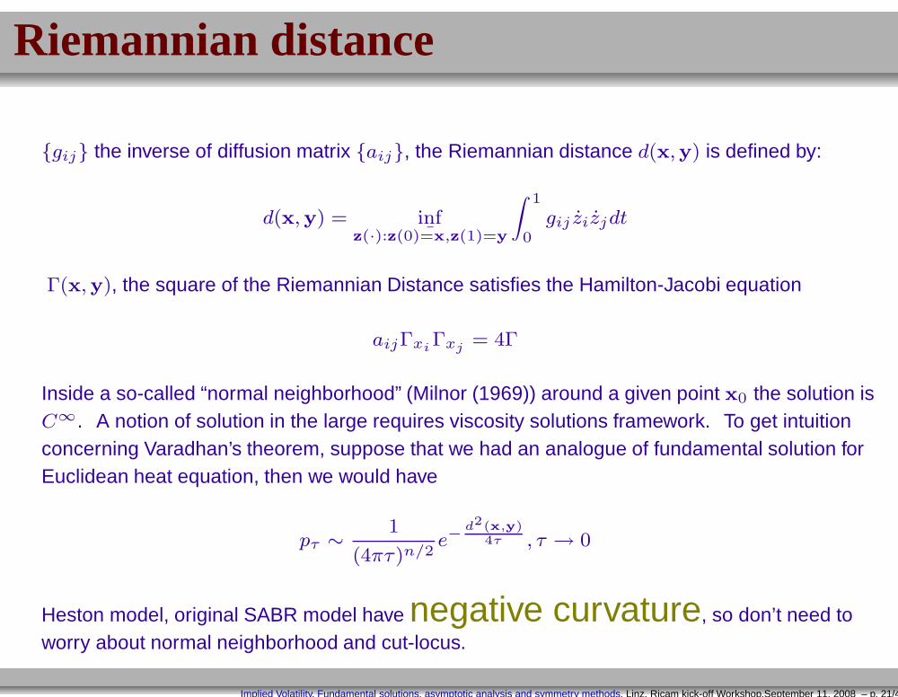
Γ(x,y), the square of the Riemannian Distance satisfies the Hamilton-Jacobi equation
aijΓxiΓxj = 4Γ
Inside a so-called “normal neighborhood” (Milnor (1969)) around a given point x0 the solution isC∞.
Implied Volatility, Fundamental solutions, asymptotic analysis and symmetry methods, Linz, Ricam kick-off Workshop,September 11, 2008 – p. 21/47

Riemannian distance
gij the inverse of diffusion matrix aij, the Riemannian distance d(x,y) is defined by:
d(x,y) = inf¯z(·):z(0)=x,z(1)=y
∫ 1
0gij zizjdt
Γ(x,y), the square of the Riemannian Distance satisfies the Hamilton-Jacobi equation
aijΓxiΓxj = 4Γ
Inside a so-called “normal neighborhood” (Milnor (1969)) around a given point x0 the solution isC∞. A notion of solution in the large requires viscosity solutions framework.
Implied Volatility, Fundamental solutions, asymptotic analysis and symmetry methods, Linz, Ricam kick-off Workshop,September 11, 2008 – p. 21/47
Riemannian distance
gij the inverse of diffusion matrix aij, the Riemannian distance d(x,y) is defined by:
d(x,y) = inf¯z(·):z(0)=x,z(1)=y
∫ 1
0gij zizjdt
Γ(x,y), the square of the Riemannian Distance satisfies the Hamilton-Jacobi equation
aijΓxiΓxj = 4Γ
Inside a so-called “normal neighborhood” (Milnor (1969)) around a given point x0 the solution isC∞. A notion of solution in the large requires viscosity solutions framework. To get intuitionconcerning Varadhan’s theorem, suppose that we had an analogue of fundamental solution forEuclidean heat equation, then we would have
pτ ∼ 1
(4πτ)n/2e−
d2(x,y)4τ , τ → 0
Heston model, original SABR model have negative curvature, so don’t need toworry about normal neighborhood and cut-locus.
Implied Volatility, Fundamental solutions, asymptotic analysis and symmetry methods, Linz, Ricam kick-off Workshop,September 11, 2008 – p. 21/47
Varadhan 2
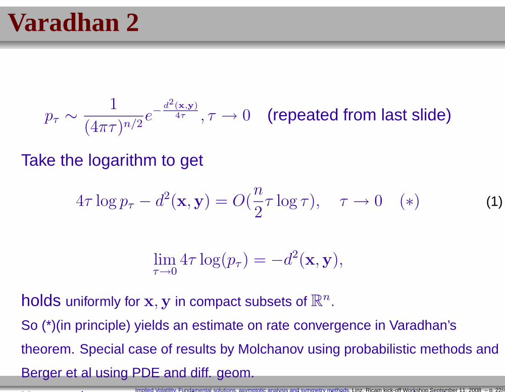
pτ ∼1
(4πτ)n/2e−
d2(x,y)4τ , τ → 0 (repeated from last slide)
Take the logarithm to get
4τ log pτ − d2(x,y) = O(n
2τ log τ), τ → 0 (∗) (1)
limτ→0
4τ log(pτ ) = −d2(x,y),
holds uniformly for x,y in compact subsets of Rn.
So (*)(in principle) yields an estimate on rate convergence in Varadhan’s
theorem. Special case of results by Molchanov using probabilistic methods and
Berger et al using PDE and diff. geom.
However, important to note that starting point in Molchanov’s analysis isImplied Volatility, Fundamental solutions, asymptotic analysis and symmetry methods, Linz, Ricam kick-off Workshop,September 11, 2008 – p. 22/47

PDE: Historical perspective
But who was the Father of it all?
Especially on PDE side?
Implied Volatility, Fundamental solutions, asymptotic analysis and symmetry methods, Linz, Ricam kick-off Workshop,September 11, 2008 – p. 23/47

Hadamard
Hadamard Portraits http://www-groups.dcs.st-and.ac.uk/~history/PictDisplay/Hadamard.html
Implied Volatility, Fundamental solutions, asymptotic analysis and symmetry methods, Linz, Ricam kick-off Workshop,September 11, 2008 – p. 24/47
Jacques Hadamard
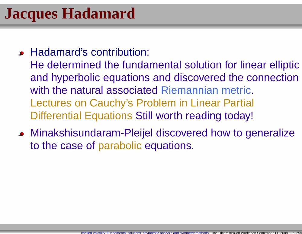
Hadamard’s contribution:He determined the fundamental solution for linear ellipticand hyperbolic equations and discovered the connectionwith the natural associated Riemannian metric.Lectures on Cauchy’s Problem in Linear PartialDifferential Equations Still worth reading today!
Minakshisundaram-Pleijel discovered how to generalizeto the case of parabolic equations.
Implied Volatility, Fundamental solutions, asymptotic analysis and symmetry methods, Linz, Ricam kick-off Workshop,September 11, 2008 – p. 25/47

Back to finance
Examples of Riemannian distances arising in finance
Local Volatility Models dFt = Ftσ(Ft) , ut − 12F 2σ2(F )uFF = 0.
d(F1, F2) =
∫ F2
F1
1
Fσ(F )dF
Implied Volatility, Fundamental solutions, asymptotic analysis and symmetry methods, Linz, Ricam kick-off Workshop,September 11, 2008 – p. 26/47

Back to finance
Examples of Riemannian distances arising in finance
Local Volatility Models dFt = Ftσ(Ft) , ut − 12F 2σ2(F )uFF = 0.
d(F1, F2) =
∫ F2
F1
1
Fσ(F )dF
SABR stochastic (alpha-beta-rho) volatility model, with β = 0, in normalized form:
dxt = −1
2y2t dt+ ytdW1t, dyt = ytdW2t, < dW1t, dW2t >= 0
Think of x = logF .
ds2 =1
y2(dx2 + dy2), y ≥ 0
We recognize this as the distance in hyperbolic plane in the Poincare model.
Implied Volatility, Fundamental solutions, asymptotic analysis and symmetry methods, Linz, Ricam kick-off Workshop,September 11, 2008 – p. 26/47
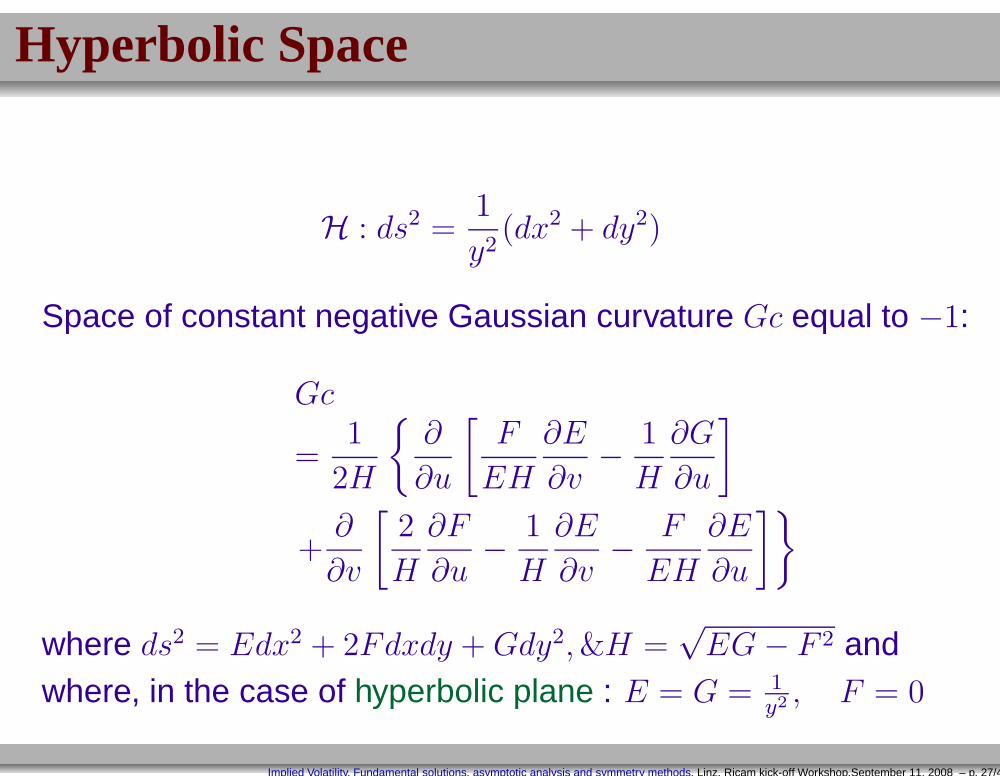
Hyperbolic Space
H : ds2 =1
y2(dx2 + dy2)
Space of constant negative Gaussian curvature Gc equal to −1:
Gc
=1
2H
∂
∂u
[F
EH
∂E
∂v− 1
H
∂G
∂u
]
+∂
∂v
[2
H
∂F
∂u− 1
H
∂E
∂v− F
EH
∂E
∂u
]
where ds2 = Edx2 + 2Fdxdy + Gdy2,&H =√
EG − F 2 andwhere, in the case of hyperbolic plane : E = G = 1
y2, F = 0
Implied Volatility, Fundamental solutions, asymptotic analysis and symmetry methods, Linz, Ricam kick-off Workshop,September 11, 2008 – p. 27/47

geodesics
2
pγ
ρ
γ through pparallels to
θ
Geodesics in the hyperbolic plane
x
y
y > 0
H
Implied Volatility, Fundamental solutions, asymptotic analysis and symmetry methods, Linz, Ricam kick-off Workshop,September 11, 2008 – p. 28/47

Geodesics in the Poincaré upper half plane model of hyperbolic space
So we need to find the geodesics in the hyperbolic plane.These are given by:
(x − a)2 + y2 = c2 semicircles centered on x axis
Boundary y = 0 is never reached, because metric blows upthere in non-integrable way.
Implied Volatility, Fundamental solutions, asymptotic analysis and symmetry methods, Linz, Ricam kick-off Workshop,September 11, 2008 – p. 29/47

Distance in hyperbolic plane and elsewhere
Setting z = (x, y), we have one can then go on to show that:
d(z1, z2) = cosh−1
(
1 +|z1 − z2|2
2y1y2
)
Implied Volatility, Fundamental solutions, asymptotic analysis and symmetry methods, Linz, Ricam kick-off Workshop,September 11, 2008 – p. 30/47

Distance in hyperbolic plane and elsewhere
Setting z = (x, y), we have one can then go on to show that:
d(z1, z2) = cosh−1
(
1 +|z1 − z2|2
2y1y2
)
Heston ModelThe mean reverting Heston model, in its traditional form (with < dW1t, dW2t >= ρdt is:
dft = ft
√V dW1t
dVt = λ(Vt − V )dt+ η√V dW2t
Let x = 12σ log f − a2
2, y = 1
2V . Associated Riemnannian metric (non-constant negative
curvature, infinite curvature at y = 0) and
ds2 =4
η2
1
y(dx2 + dy2) =
4y
η2
︸︷︷︸
conformal factor
ds2H2
︸ ︷︷ ︸
hyperbolic metric
So Heston model, in the new coordinates is in the same conformal class as hyperbolic plane.Implied Volatility, Fundamental solutions, asymptotic analysis and symmetry methods, Linz, Ricam kick-off Workshop,September 11, 2008 – p. 30/47
geodesics Heston model
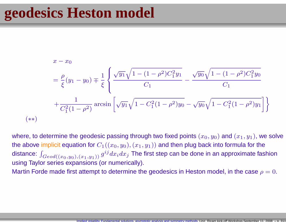
x− x0
=ρ
ξ(y1 − y0) ∓ 1
ξ
√y1
√
1 − (1 − ρ2)C21y1
C1−
√y0
√
1 − (1 − ρ2)C21y0
C1
+1
C21 (1 − ρ2)
arcsin
[√y1
√
1 − C21 (1 − ρ2)y0 −√
y0
√
1 − C21 (1 − ρ2)y1
]
(∗∗)
where, to determine the geodesic passing through two fixed points (x0, y0) and (x1, y1), we solvethe above implicit equation for C1((x0, y0), (x1, y1)) and then plug back into formula for thedistance:
∫
Geod((x0,y0),(x1,y1)) gijdxidxj The first step can be done in an approximate fashion
using Taylor series expansions (or numerically).Martin Forde made first attempt to determine the geodesics in Heston model, in the case ρ = 0.
Implied Volatility, Fundamental solutions, asymptotic analysis and symmetry methods, Linz, Ricam kick-off Workshop,September 11, 2008 – p. 31/47

Heat kernel Series solution for fundamental solution
Seek solution in the form of a series:
F (x, y, τ) =
√
g(x)
(2πτ)n/2
√
∆(x, y)P(x, y)e−d2(x,y)
2τ
+∞∑
n=1
un(x, y)τn, τ → 0
Implied Volatility, Fundamental solutions, asymptotic analysis and symmetry methods, Linz, Ricam kick-off Workshop,September 11, 2008 – p. 32/47

Heat kernel Series solution for fundamental solution
Seek solution in the form of a series:
F (x, y, τ) =
√
g(x)
(2πτ)n/2
√
∆(x, y)P(x, y)e−d2(x,y)
2τ
+∞∑
n=1
un(x, y)τn, τ → 0
where,
d(x, y) is the geodesic distance between x and y, i.e., minimizer of the functional
∫ 1
0gij
dxi
dt
dxj
dtdt
x(0) = x x(1) = y,
where recall:
g = a−1, where a = aij is principle part of elliptic operator aij∂2
∂xi∂xj
Implied Volatility, Fundamental solutions, asymptotic analysis and symmetry methods, Linz, Ricam kick-off Workshop,September 11, 2008 – p. 32/47

Heat kernel ct’d
fτ − aij∂2
∂xi∂xjf − bi
∂
∂xif = 0
Solution in the form :√
g(x)
(4πτ)n/2
√
∆(x, y)P(x, y)e−d2(x,y)
4τ
+∞∑
n=1
an(x, y)τn, τ → 0
∆(x, y) = |g(x)|−1/2det
∂ d2
2
∂x∂y
|g(y)|−1/2 Van-Vleck-DeWitt determinant
P = exponential of work done by fieldA, e∫
C(x,y) A·dl
A is constructed from PDE, using two ingredients: principle part and from the drift b, i.e.
Ai = bi − det(g)−1/2 ∂
∂xj
(
det(g)1/2gij)
Implied Volatility, Fundamental solutions, asymptotic analysis and symmetry methods, Linz, Ricam kick-off Workshop,September 11, 2008 – p. 33/47

Heat kernel
√
g(x)
(4πτ)n/2
√
∆(x, y)P(x, y)e−d2(x,y)
4τ
+∞∑
n=1
un(x, y)τn, τ → 0
Characterization of heat kernel coefficients
Obtained via a recursive scheme:
u0(x, y) = 1
(1 +1
k
[∇id2
])∇i)uk = P−1∆−1/2LS∆1/2Puk−1
ordinary differential equations along geodesics, ie. in WKB known as “transport equations”
∇i = ∂i + Ai
.
Implied Volatility, Fundamental solutions, asymptotic analysis and symmetry methods, Linz, Ricam kick-off Workshop,September 11, 2008 – p. 34/47

Simplest Case
√
g(x)
(4πτ)n/2
√
∆(x, y)P(x, y)e−d2(x,y)
4τ
+∞∑
n=1
an(x, y)τn, τ → 0
Laborious calculations by a host of mathematicians and physicists characterize theon-diagonal form of the heat kernel coefficients, ie. we have
u0(x, x) = 1
u1(x, x) = P =1
6Scalar Curvature + gij(AiAj − bjAi −
∂
∂xjAi)
︸ ︷︷ ︸
Q
u2(x, x) =1
180
(|Riemann Tensor|2 − |Ricci Tensor|2
)+
1
2a21 +
1
2|R|2
+1
30∆BelR+
1
6Q
Implied Volatility, Fundamental solutions, asymptotic analysis and symmetry methods, Linz, Ricam kick-off Workshop,September 11, 2008 – p. 35/47

Discussion
First few terms in the series very effective as revealed bynumerical experiments comparing approximatingsolution to numerically computed solution. Numericalexamples later, time permitting.
However, expansions not rigorously justified (-able ?)without suitable adjustment of the expansion.
Implied Volatility, Fundamental solutions, asymptotic analysis and symmetry methods, Linz, Ricam kick-off Workshop,September 11, 2008 – p. 36/47

Adjustments in analytic/diff.geometric approach
PDE approach due to Minakshisundaram-Pleijel( See Berger-Gauduchon-Mazet). Idea:construct a parametrix (defin. of "parametrix" on next slide), via a series in two stages(assume Laplace-Beltrami for simplicity)Stage 1): Geometric Stage , for close points: Essentially same as above-mentionedasymptotic ansatz.
Fundamental Solution F =1
(4πτ)n/2e−d2(x,y)/4τ
∞∑
i=0
ui(x, y)τn
Ie. Use transport equns to determine coeffts. But now
Stage 2) To define globally, ie. for distant points, 1) truncate series for any k > n2
(usinggeometrically determined coefficients for n < k/2) and 2) use cut-off function away from thediagonal:I.e: Let ρ be smooth cut-off with ρ(0, ǫ/4) = 1, ρ(ǫ/2,∞) = 0. Consider
Hk = ρ(d(x, y))1
(4πτ)n/2e−d2(x,y)/4τ
k∑
i=0
ui(x, y)τn
.
Implied Volatility, Fundamental solutions, asymptotic analysis and symmetry methods, Linz, Ricam kick-off Workshop,September 11, 2008 – p. 37/47

Parametrix
Can show that this is parametrix ie.
(∂τ − LS)
ρ(d(x, y))
[
1(4πτ)n/2 e
−d2(x,y)
4τ
k∑
i=0ui(x, y)τ
i
]
= O(tk−n2 )e−d2(x,y)/2tGk
where Gk is smooth.
Use Levy parametrix idea (iterated convolution) to push error off to infinity. Ie.
Fundamental Solution = Hk + Hk ∗ F
where
F ∗G(x, y, t) =
∫ t
0
∫
MF (x, z, τ)G(z, y, t− τ)dV (z)
and where, letting L = ∂t − LS ,
F =∞∑
l=1
(LHk)∗l
Iterated (infinitely) convolution.
Implied Volatility, Fundamental solutions, asymptotic analysis and symmetry methods, Linz, Ricam kick-off Workshop,September 11, 2008 – p. 38/47
Adjustments 2
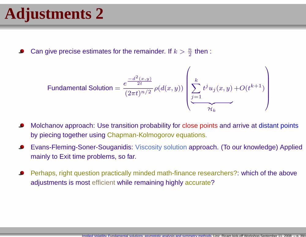
Can give precise estimates for the remainder. If k > n2
then :
Fundamental Solution =e
−d2(x,y)2t
(2πt)n/2ρ(d(x, y))
k∑
j=1
tjuj(x, y)
︸ ︷︷ ︸
Hk
+O(tk+1)
Molchanov approach: Use transition probability for close points and arrive at distant pointsby piecing together using Chapman-Kolmogorov equations.
Evans-Fleming-Soner-Souganidis: Viscosity solution approach. (To our knowledge) Appliedmainly to Exit time problems, so far.
Perhaps, right question practically minded math-finance researchers?: which of the aboveadjustments is most efficient while remaining highly accurate?
Implied Volatility, Fundamental solutions, asymptotic analysis and symmetry methods, Linz, Ricam kick-off Workshop,September 11, 2008 – p. 39/47

Influence of curvature
G. Ben Arous, P.L., TH Wang
Theorem 1 Consider the SV model
dxt = b(xt)ytdW1t + µdt
dyt = γyq+1t dW2t + νdt
< dW1t, dW2t >= ρdt
where ρ and γ are constants. Then
The curvature of the Riemannian metric naturally associated to the problem is independent ofthe factor b(x) and independent of the correlation and of the drift.
The curvature is equal to
(q − 1)y2q
Thus
The curvature is identically zero if and only if q = 1 , ie. in the quadratic case, and isnegative when q < 1.
Implied Volatility, Fundamental solutions, asymptotic analysis and symmetry methods, Linz, Ricam kick-off Workshop,September 11, 2008 – p. 40/47

influence of curvature II
When q = 0, the curvature is constant.This is the original lognormal Sabr model.
When q = −1 i.e. Heston model, the curvature isnegative and it blows up at y = 0. In fact the curvatureblows up at y = 0 as soon as q < 0.
Note; The sign and size of the curvature is important inthe heat kernel asymptotic approach to the heat kernel.Here is why:The first reason is geometric and has analyticcorrolaries: On Riemannian manifolds of negativeRiemannian curvature, the cut locus is empty.
Implied Volatility, Fundamental solutions, asymptotic analysis and symmetry methods, Linz, Ricam kick-off Workshop,September 11, 2008 – p. 41/47
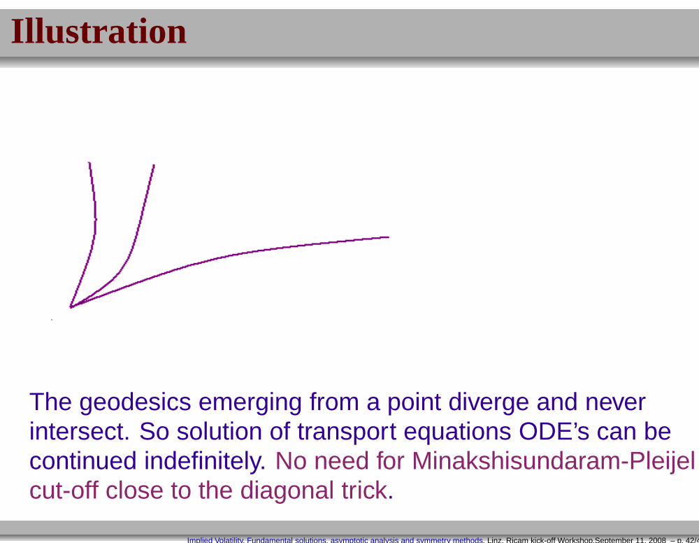
Illustration
The geodesics emerging from a point diverge and neverintersect. So solution of transport equations ODE’s can becontinued indefinitely. No need for Minakshisundaram-Pleijelcut-off close to the diagonal trick.
Implied Volatility, Fundamental solutions, asymptotic analysis and symmetry methods, Linz, Ricam kick-off Workshop,September 11, 2008 – p. 42/47
Influence of Curvature on asymptotics
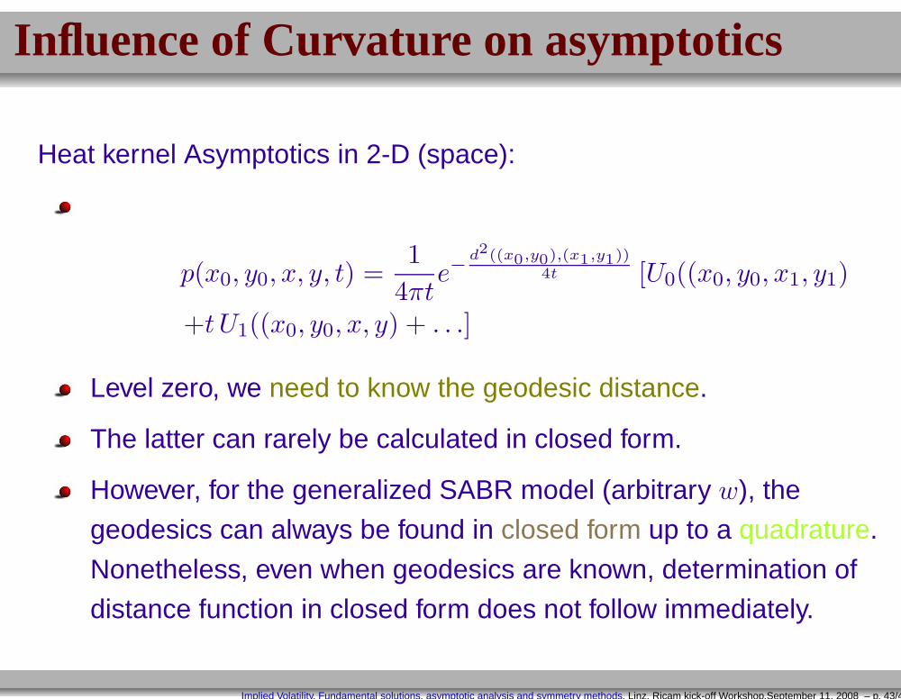
Heat kernel Asymptotics in 2-D (space):
p(x0, y0, x, y, t) =1
4πte−
d2((x0,y0),(x1,y1))4t [U0((x0, y0, x1, y1)
+t U1((x0, y0, x, y) + . . .]
Level zero, we need to know the geodesic distance.
The latter can rarely be calculated in closed form.
However, for the generalized SABR model (arbitrary w), the
geodesics can always be found in closed form up to a quadrature.
Nonetheless, even when geodesics are known, determination of
distance function in closed form does not follow immediately.
Implied Volatility, Fundamental solutions, asymptotic analysis and symmetry methods, Linz, Ricam kick-off Workshop,September 11, 2008 – p. 43/47

Influence of curvature
Recall that when q ≤ 0 (as in Heston model, where q = −1), the curvature blows up aty = 0.But leading order term in order 1, ie. U1 coefficient in heat kernel expansion, is :
U1(x, x) =1
3K +Q ∼ C
y2+Q in Heston model
ie., we have
F (x, y) =1
4πte−d2/4t (U0(x, y) + U1(x, y)t+ · · · )
so, we see that U1 term in expansion cannot be accurate for y with y2t = O(1). Needsadjustment: boundary layer, otherwise need to take t tremendously small, close to y = 0.
Implied Volatility, Fundamental solutions, asymptotic analysis and symmetry methods, Linz, Ricam kick-off Workshop,September 11, 2008 – p. 44/47

Need for Distance function
The heat kernel approach requires, as we have seen, theevaluation of Riemannian distance function. So,what to do,when this distance function is not known in closed form?
Alternatives are:
Determine Riemannian distance numerically, by solving theeikonal equation:
gijdxidxj
= 1, (i.e. |grad d| = 1)
or
Find a larger class of SV models for which d can bedetermined in closed or in semi-closed form.
In order to determine the latter, one can try and find allImplied Volatility, Fundamental solutions, asymptotic analysis and symmetry methods, Linz, Ricam kick-off Workshop,September 11, 2008 – p. 45/47

First Order system of linear equations
To determine the symmetries, need to find infinitesimal generators of vector fields:
V = ξ∂
∂x+ η
∂
∂y︸ ︷︷ ︸
generator of spatial variation
+ φ∂
∂u︸ ︷︷ ︸
change of dependent variable
These satisfy an overdetermined system of first order partial differential equations, such as
five equations
Aφx +Bφy = ξu
Bφx + Cφy = ηu
2ACξx + 2BCξy − 2ABηx − 2ACηy + (ACx −AxC)ξ + · · · = 0
. . . . . .
. . . . . .
Implied Volatility, Fundamental solutions, asymptotic analysis and symmetry methods, Linz, Ricam kick-off Workshop,September 11, 2008 – p. 46/47
Conclusion
Various approaches to short time asymptotics exist in the literaure. A detailed comparison ofthe efficiency and accuracies of these is an important and open problem.
For the heat kernel approach, we are essentially at the beginning of exploring it’s potential.This is because so far it has only been considered in detail in cases where the distancefunction is known in closed form.
Optimally combining the parametrix approach with the geometric approach is an issue to beexplored in depth in the future.
Influence of off-diagonal corrections on asymptotic implied volatility formulas is an openproblem.
Asymptotics taking into account Dirichlet (barrier options) and Neumann boundaryconditions unexplored so far.
Implied Volatility, Fundamental solutions, asymptotic analysis and symmetry methods, Linz, Ricam kick-off Workshop,September 11, 2008 – p. 47/47