Implicit solution techniques for coupledmulti-field problems –

Block Solution, Coupled MatricesHenrik Rusche and Hrvoje Jasak

h.rusche@wikki-gmbh.de, h.jasak@wikki.co.uk

Wikki, Germany and United Kingdom

Advanced Training at the OpenFOAM Workshop

23.6.2010, Gothenburg, Sweden

Implicit solution techniques for coupled multi-field problems –Block Solution, Coupled Matrices – p. 1

Background

Objective

• Review of coupling methodologies

Topics

1. Motivation and Overview

2. Multi Domain Support

3. Domain Coupled Solution Algorithmns: Coupled Matrices

4. Equation Coupled Solution Algorithmns: Block Matrices

5. Summary

Implicit solution techniques for coupled multi-field problems –Block Solution, Coupled Matrices – p. 2

Motivation and Overview

• Coupled solution algorithms are designed to handle systems of equations in themost efficient way possible

• The option of solving all equations together always exists, but it is very expensiveand in most cases unnecessary

• The objective is to treat “important” and “nice” terms implicitly and handle thecoupling algorithmically whenever possible

• Numerically well behaved terms help with the stability of discretisation

• But in some cases explicit coupling simply does not work or it is too slow

• Today : Emphasis on Implicit Coupling

◦ Domain (Matrix) coupling

◦ Equation (Block) coupling

Implicit solution techniques for coupled multi-field problems –Block Solution, Coupled Matrices – p. 3

Domain Coupling Test Case

• Steady-state conjugate heat transfer to an incompressible, laminar fluid

• Fluid: ∇•(uu)−∇•ν∇u = −∇p (1)

∇•u = 0 (2)

∇•(uT )−∇•K(∇T ) = 0 (3)

• Solid: −∇•Ks(∇Ts) = 0 (4)

• Interface: T = Ts (5)

K∇T = Ks∇Ts (6)

Implicit solution techniques for coupled multi-field problems –Block Solution, Coupled Matrices – p. 4

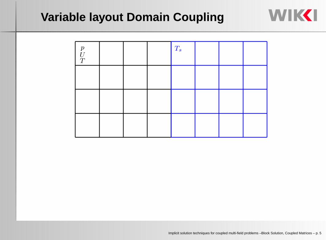
Variable layout Domain Coupling

pUT

Ts

Implicit solution techniques for coupled multi-field problems –Block Solution, Coupled Matrices – p. 5

Multiple Domain Support

Multiple Domains in a Single Simulation

• Original class-based design allows for multiple object of the same type in a singlesimulation, e.g. meshes and fields

• Solution: hierarchical object registry◦ Multiple named mesh databases within a single simulation:

1 mesh = 1 domain, with separate fields and physics

◦ Fields, material properties and solution controls separate for each mesh

• “Main” mesh controls time advancement (with possible sub-cycling)

Code Organisation

• Every individual mesh represents a single addressing space , with its owninternal faces and boundaries. Operations on various face types are consistent:consequences for conjugate heat transfer type of coupling

Implicit solution techniques for coupled multi-field problems –Block Solution, Coupled Matrices – p. 6

Multiple Domain Support

Case Organisation for Multiple Meshes: “Main Mesh” and solid

system

constant

points

cells

faces

boundary

polyMesh

. . . Properties

solid

solid

fvSchemes

fvSolution

U

T

solid

<case>

boundary

time directories

controlDict

fvSchemes

fvSolution

polyMesh

points

cells

faces

. . . Properties

U

p

Implicit solution techniques for coupled multi-field problems –Block Solution, Coupled Matrices – p. 7

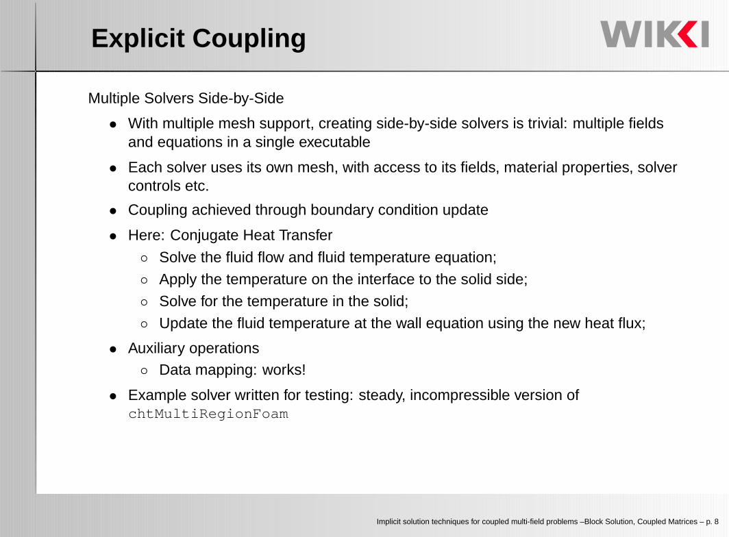
Explicit Coupling

Multiple Solvers Side-by-Side

• With multiple mesh support, creating side-by-side solvers is trivial: multiple fieldsand equations in a single executable

• Each solver uses its own mesh, with access to its fields, material properties, solvercontrols etc.

• Coupling achieved through boundary condition update

• Here: Conjugate Heat Transfer

◦ Solve the fluid flow and fluid temperature equation;

◦ Apply the temperature on the interface to the solid side;

◦ Solve for the temperature in the solid;

◦ Update the fluid temperature at the wall equation using the new heat flux;

• Auxiliary operations◦ Data mapping: works!

• Example solver written for testing: steady, incompressible version ofchtMultiRegionFoam

Implicit solution techniques for coupled multi-field problems –Block Solution, Coupled Matrices – p. 8

Implicit Domain (Matrix) Coupling

• In many cases, Picard iterations (explicit coupling) simply does not work or it is tooslow

• Discretisation machinery in OpenFOAM is satisfactory and needs to be preserved

• Multi-domain support must allow for some variables/equations to be coupled, whileothers remain separated

• Example: conjugate heat transfer

◦ Fluid flow equations solved on fluid only

◦ Energy equation discretised separately on the fluid and solid region but solvedin a single linear solver call

• Combining variables or addressing spaces into implicit coupling requires specialpractices and tools

• Historically, conjugate heat transfer in many CFD codes is “hacked” as a specialcase: we need a general arbitrary matrix-to-matrix coupling

• The problem was insufficient flexibility of matrix support

Implicit solution techniques for coupled multi-field problems –Block Solution, Coupled Matrices – p. 9

Implementation of Domain Coupling

• OpenFOAM supports multi-region simulations, with possibility of separateaddressing and physics for each mesh: multiple meshes, with local fields

• Some equations present only locally, while others span multiple meshes

coupledFvScalarMatrix TEqns(2);

TEqns.hook(

fvm::ddt(T) + fvm::div(phi, T)- fvm::laplacian(DT, T)

);

TEqns.hook(

fvm::ddt(Tsolid) - fvm::laplacian(DTsolid, Tsolid));

TEqns.solve();

• Matrix coupled solver handles multiple matrices together in internal solver sweeps

Implicit solution techniques for coupled multi-field problems –Block Solution, Coupled Matrices – p. 10

Mesh and Matrix for Domain Coupling

T1 T2 Ts1 Ts2

a ·

·. . .

·

·

a ·

·. . .

T1

...Ts1

...

=

b2

...bs1

...

(7)

Implicit solution techniques for coupled multi-field problems –Block Solution, Coupled Matrices – p. 11

Domain Coupled Solution Algorithms

Example: Conjugate Heat Transfer

• Coupling may be established geometrically: adjacent surface pairs

• Each variable is stored only on a mesh where it is active: (U, p, T)

• Choice of conjugate variables is completely arbitrary: e.g. catalytic reactions

• Coupling is established only per-variable: handling a general coupled complexphysics problem rather than conjugate heat transfer problem specifically

Implicit solution techniques for coupled multi-field problems –Block Solution, Coupled Matrices – p. 12

Results: Domain Coupling Test Case

0 100 200 300 400Iterations [-]

10-5

10-4

10-3

10-2

10-1

100

max

rel

ativ

e er

ror

[-]

segregated solution Tsegregated solution Tsmatrix coupled solution Tmatrix coupled solution Ts

conjugateCavity

Implicit solution techniques for coupled multi-field problems –Block Solution, Coupled Matrices – p. 13

Equation Coupling Test Case

• Steady-state conjugate heat transfer between a porous medium and a fluid flowingthrough it - Frozen flow field

• Fluid: ∇•(uT )−∇•K(∇T ) = α(Ts − T ) (8)

• Solid: −∇•Ks(∇Ts) = α(T − Ts) (9)

• Frozen flow field: u = (0, 0,−1)× (x− x0) (10)

Implicit solution techniques for coupled multi-field problems –Block Solution, Coupled Matrices – p. 14

Variable Layout Domain Coupling

T1 T2

Ts1 Ts2

Implicit solution techniques for coupled multi-field problems –Block Solution, Coupled Matrices – p. 15

Segregated Algorithmn

• Trivial: This is what OpenFOAM was designed for!

fvScalarMatrix TEqn(

fvm::div(phi, T)- fvm::laplacian(DT, T)==

alpha*Ts - fvm::Sp(alpha, T));

TEqn.relax(); TEqn.solve();

fvScalarMatrix TsEqn(

- fvm::laplacian(DTs, Ts)==

alpha*T - fvm::Sp(alpha, Ts));

TsEqn.relax(); TsEqn.solve();

Implicit solution techniques for coupled multi-field problems –Block Solution, Coupled Matrices – p. 16

Equation Coupling Idea

• How to couple implicitly?

• Think vectorial at each cell! x =

[

T

Ts

]

• Matrix coefficients become tensors ... How does this look like?

Implicit solution techniques for coupled multi-field problems –Block Solution, Coupled Matrices – p. 17

Mesh and Matrix Equation (Block)Coupling

T1 T2

Ts1 Ts2

(

aff afs

asf ass

)

. · · ·

.

(

aff afs

asf ass

)

· · ·

......

. . .

T1

Ts1

T1

Ts2

...

=

b1

bs1

b2

bs2

...

(11)

Implicit solution techniques for coupled multi-field problems –Block Solution, Coupled Matrices – p. 18

Block Coupled Solution Algorithms

Block Matrix Implementation

• Implementation is general and includes off-diagonal coefficients

• Arbitrary number of equations can be coupled. aP and aN may be n× n tensors

• For vector components coupled in the same cell, aP is a tensor

• For a vector cross-coupled to its neighbourhood, (e.g. x-to-y), aN is a tensor

• Matrix algebra generalises to block coefficients, including linear solvers

• . . . and global sparseness pattern of the matrix is still dictated by the mesh!

• For efficiency, coefficient arrays are morphed: scalar->linear->square type

Implicit solution techniques for coupled multi-field problems –Block Solution, Coupled Matrices – p. 19

Results: Equation Coupling Test Case

0 100 200 300Iteration [-]

10-4

10-3

10-2

10-1

100

max

ium

um r

elat

ive

erro

r [-

]segregated solution Tsegregated solution Tsblock coupled solution Tblock coupled solution Ts

2-eq swirlTest

Implicit solution techniques for coupled multi-field problems –Block Solution, Coupled Matrices – p. 20

Summary

Domain (Matrix) Coupling:

• List of matrices for each coupled component mesh

• Coupled boundary condition, where the coupling may be established on aper-variable basis

• Set of new multi-matrix solvers: all algorithms generalise without issues

• Substantial improvements in convergence on simple test case

• Expecting similiar performance to closed-source CHT codes

• Arbitrary equations and variables can be coupled on demand: much better thatplain-vanilla conjugate heat transfer!

Equation (Block) Coupling:

• Block matrix classes implemented and tested. Memory usage, solver efficiencyand performance satisfactory compared to segregated solver

• Block solver used in isolation in a project on strongly coupled equation sets

• Block coefficients created by combining single equation discretisation, addingcross-component coupling terms “by hand”

• Needs improvements on ease-of-use: re-basing discretisation classes

• Substantial improvements in convergence on simple test case

Implicit solution techniques for coupled multi-field problems –Block Solution, Coupled Matrices – p. 21

Status of Block Matrix Implementation

• Block matrix classes implemented and tested. Memory usage, solver efficiencyand performance satisfactory compared to segregated solver

• Block solver used in isolation in a project on strongly coupled equation sets

◦ Learning lessons on solver pre-conditioning and equation coupling

◦ Block coefficients created combining single equation discretisation, addingcross-component coupling terms “by hand”

◦ Needs improvements on ease-of-use: re-basing discretisation classes

• Discretisation support : Block FVM and FEM

◦ Software improvement: significantly simpler and more efficient fvMatrix

◦ FEM solver re-based on block matrix: linear stress analysis in one solver call!

◦ FVM discretisation re-based on block matrix and tested on simple flows

◦ Current work: discretisation of special component-coupled FVM operators∗ Div-grad-T term ∇•(γ∇u

T ): fvm::laplacianTranspose(gamma, U):∗ Adjoint convection term U•∇v: fvm::divTranspose(U, V)

• Next steps: Towards an implicit block-coupled density-based solver◦ Further testing and validation

◦ Re-activate parallelisation and release test library

Implicit solution techniques for coupled multi-field problems –Block Solution, Coupled Matrices – p. 22