Implementing quantum gates andchannels using linear optics

by

Kent Fisher

A thesispresented to the University of Waterloo

in fulfillment of thethesis requirement for the degree of

Master of Sciencein

Physics - Quantum Information

Waterloo, Ontario, Canada, 2012

c© Kent Fisher 2012

I hereby declare that I am the sole author of this thesis. This is a true copy of the thesis,including any required final revisions, as accepted by my examiners.

I understand that my thesis may be made electronically available to the public.

ii

Abstract

This thesis deals with the implementation of quantum channels using linear optics. Webegin with overviews of some important concepts in both quantum information and quan-tum optics. First, we discuss the quantum bit and describe the evolution of the states viaquantum channels. We then discuss both quantum state and process tomography, methodsfor how to determine which states and operations we are experimentally implementing inthe lab. Second, we discuss topics in quantum optics such the generation of single photons,polarization entanglement, and the construction of an entangling gate.

The first experiment is the implementation of a quantum damping channel, whichintentionally can add a specific type and amount of decohering noise to a photonic qubit.Specifically, we realized a class of quantum channels which contains both the amplitude-damping channel and the bit-flip channel, and did so with a single, static, optical setup.Many quantum channels, and some gates, can only be implemented probabilistically whenusing linear optics and postselection. Our main result is that the optical setup achieves theoptimal success probability for each channel. Using a novel ancilla-assisted tomography,we characterize each case of the channel, and find process fideilities of 0.98± 0.01 for theamplitude-damping channel and 0.976± 0.009 for the bit-flip.

The second experiment is an implementation of a protocol for quantum computing onencrypted data. The protocol provides the means for a client with very limited quantumpower to use a server’s quantum computer while maintaining privacy over the data. Weperform a quantum process tomography for each gate in a universal set, showing that onlywhen the proper decryption key is used on the output states, which is hidden from theserver, then the action of the quantum gate is recovered. Otherwise, the gate acts as thecompletely depolarizing channel.

iii

Acknowledgements

First, I would like to thank my supervisor Kevin Resch. He is a fantastic physicist andteacher, and I am very grateful to have been able to study and research under his guidance.I am excited to continue working in his group during my PhD. I would like to thank theother members of my advising committee, Norbert Lutkenhaus and Joseph Sanderson, aswell as Raymond Laflamme for sitting on my examining committee.

Laboratory research is very much a team sport, and so I would like to thank the othermembers of the Quantum Information and Quantum Optics group, both past and present,for their continual help in the lab. I thank Jonathon Lavoie, Deny Hamel, Krister Shalmand Robert Prevedel for their advice and patience as I learned the ins and outs of quantumoptics experiments. I would also like thank Mike Mazurek, John Donahue and Chris Erven,who are always glad to help out and bounce ideas off of.

During the second half of my Master’s, I performed the experiment for a protocoldesigned by Anne Broadbent. I would like to thank Anne for her help as I learned the finerdetails of the protocol, and also for her patience with the inevitable delays that accompanyexperiments.

On countless occasions I have needed technical help with certain components in thelab. Rainer Kaltenbaek deserves thanks for laying so much of the groundwork in the lab,particularly with LabView coding. He continues to help from afar. Also, Zhizhong Yantirelessly helped me in setting up the Pockels cells. It is a very frustrating job, and I amvery grateful to him.

I would like to acknowledge the agencies which have provided funding for the exper-iments which I have been able to work on. These are Ontario Ministry of Research andInnovation ERA, QuantumWorks, NSERC, OCE, Industry Canada and CFI. I would alsolike to thank NSERC and OGS, who personally funded me during my Master’s.

Lastly, I would like to thank my family and friends. Their goodness and prayers havecarried me through both joyful and hard times. I treasure their love and support.

iv

By wisdom a house is built, and through understanding it is established; throughknowledge its rooms are filled with rare and beautiful treasures.

– Proverbs 24:3-4

If I can fathom all mysteries and all knowledge but do not have love, then I am nothing.

– 1 Corinthians 13:2

My goal is that we may be encouraged in heart and united in love, so that we may havethe full riches of complete understanding, in order that we might know the mystery ofGod, namely Christ, in whom are hidden all the treasures of wisdom and knowledge.

– Colossians 2:2-3

v

Table of Contents

List of Figures ix

1 Quantum Information Background 1

1.1 Introduction . . . . . . . . . . . . . . . . . . . . . . . . . . . . . . . . . . . 1

1.2 The Qubit . . . . . . . . . . . . . . . . . . . . . . . . . . . . . . . . . . . . 2

1.3 Entanglement . . . . . . . . . . . . . . . . . . . . . . . . . . . . . . . . . . 3

1.4 Quantum channels . . . . . . . . . . . . . . . . . . . . . . . . . . . . . . . 4

1.4.1 Kraus representation . . . . . . . . . . . . . . . . . . . . . . . . . . 5

1.4.2 Superoperator representation . . . . . . . . . . . . . . . . . . . . . 6

1.4.3 Choi matrix representation . . . . . . . . . . . . . . . . . . . . . . . 6

1.5 Quantum state tomography . . . . . . . . . . . . . . . . . . . . . . . . . . 7

1.5.1 Maximum likelihood . . . . . . . . . . . . . . . . . . . . . . . . . . 8

1.5.2 Monte Carlo error analysis . . . . . . . . . . . . . . . . . . . . . . . 9

1.6 Quantum process tomography . . . . . . . . . . . . . . . . . . . . . . . . . 9

1.6.1 Maximum likelihood . . . . . . . . . . . . . . . . . . . . . . . . . . 10

1.6.2 Ancilla-assisted process tomography . . . . . . . . . . . . . . . . . . 11

1.6.3 Monte Carlo error analysis . . . . . . . . . . . . . . . . . . . . . . . 11

1.7 Distance measures . . . . . . . . . . . . . . . . . . . . . . . . . . . . . . . 11

1.7.1 State fidelity . . . . . . . . . . . . . . . . . . . . . . . . . . . . . . . 11

1.7.2 Process fidelity . . . . . . . . . . . . . . . . . . . . . . . . . . . . . 12

1.7.3 Trace distance . . . . . . . . . . . . . . . . . . . . . . . . . . . . . . 12

vi

2 Quantum optics background 14

2.1 Introduction . . . . . . . . . . . . . . . . . . . . . . . . . . . . . . . . . . . 14

2.2 Generation of single photon entangled states . . . . . . . . . . . . . . . . . 15

2.2.1 Spontaneous parametric downconversion . . . . . . . . . . . . . . . 15

2.2.2 Phase matching . . . . . . . . . . . . . . . . . . . . . . . . . . . . . 18

2.2.3 Polarization entanglement . . . . . . . . . . . . . . . . . . . . . . . 19

2.3 The beamsplitter and Hong-Ou-Mandel interference . . . . . . . . . . . . . 20

2.4 Pockels cells . . . . . . . . . . . . . . . . . . . . . . . . . . . . . . . . . . . 22

2.5 Optical CNOT gate . . . . . . . . . . . . . . . . . . . . . . . . . . . . . . . 23

2.5.1 Partially-polarizing beamsplitters . . . . . . . . . . . . . . . . . . . 24

2.5.2 Using the PPBS to generate entanglement . . . . . . . . . . . . . . 26

2.5.3 Experimental setup . . . . . . . . . . . . . . . . . . . . . . . . . . . 28

2.5.4 Results . . . . . . . . . . . . . . . . . . . . . . . . . . . . . . . . . . 28

3 Optimal linear optical implementation of a single-qubit damping channel 30

3.1 Notes and acknowledgements . . . . . . . . . . . . . . . . . . . . . . . . . 30

3.2 Abstract . . . . . . . . . . . . . . . . . . . . . . . . . . . . . . . . . . . . . 31

3.3 Introduction . . . . . . . . . . . . . . . . . . . . . . . . . . . . . . . . . . . 31

3.4 Optimality of the implementation . . . . . . . . . . . . . . . . . . . . . . . 33

3.5 Ancilla-assisted process tomography . . . . . . . . . . . . . . . . . . . . . . 33

3.6 Experiment . . . . . . . . . . . . . . . . . . . . . . . . . . . . . . . . . . . 34

3.7 Results . . . . . . . . . . . . . . . . . . . . . . . . . . . . . . . . . . . . . . 36

3.8 Summary . . . . . . . . . . . . . . . . . . . . . . . . . . . . . . . . . . . . 39

4 Quantum computing on encrypted data 40

4.1 Notes and acknowledgements . . . . . . . . . . . . . . . . . . . . . . . . . 40

4.2 Introduction . . . . . . . . . . . . . . . . . . . . . . . . . . . . . . . . . . . 41

4.3 Protocol . . . . . . . . . . . . . . . . . . . . . . . . . . . . . . . . . . . . . 43

vii

4.4 Experiment . . . . . . . . . . . . . . . . . . . . . . . . . . . . . . . . . . . 45

4.5 Summary . . . . . . . . . . . . . . . . . . . . . . . . . . . . . . . . . . . . 48

4.6 Methods . . . . . . . . . . . . . . . . . . . . . . . . . . . . . . . . . . . . . 48

4.7 Supplementary Information . . . . . . . . . . . . . . . . . . . . . . . . . . 49

4.7.1 Correctness of the R-gate protocol . . . . . . . . . . . . . . . . . . . 49

4.7.2 Security definition and proof . . . . . . . . . . . . . . . . . . . . . . 50

5 Conclusion 56

APPENDICES 57

A Configuring Pockels cells 58

B Imperfection in the CNOT gate 64

B.1 Imperfect interference . . . . . . . . . . . . . . . . . . . . . . . . . . . . . . 64

References 68

viii

List of Figures

1.1 The Bloch sphere . . . . . . . . . . . . . . . . . . . . . . . . . . . . . . . . 3

1.2 Amplitude damping on the Bloch sphere . . . . . . . . . . . . . . . . . . . 7

2.1 Polarization of light . . . . . . . . . . . . . . . . . . . . . . . . . . . . . . . 15

2.2 Spontaneous parametric downconversion . . . . . . . . . . . . . . . . . . . 18

2.3 Quasi-phase matching . . . . . . . . . . . . . . . . . . . . . . . . . . . . . 19

2.4 Sagnac source . . . . . . . . . . . . . . . . . . . . . . . . . . . . . . . . . . 20

2.5 HOM interferometer . . . . . . . . . . . . . . . . . . . . . . . . . . . . . . 21

2.6 Optical setup for the CNOT gate . . . . . . . . . . . . . . . . . . . . . . . 25

2.7 Measured HOM dip . . . . . . . . . . . . . . . . . . . . . . . . . . . . . . . 26

2.8 Bell state output from CNOT gate . . . . . . . . . . . . . . . . . . . . . . 28

3.1 Experimental setup for the damping channel . . . . . . . . . . . . . . . . . 35

3.2 Success probability and tangle results . . . . . . . . . . . . . . . . . . . . . 37

3.3 Process fidelity and trace distance results . . . . . . . . . . . . . . . . . . . 38

4.1 Cloud computing . . . . . . . . . . . . . . . . . . . . . . . . . . . . . . . . 42

4.2 Encryptions on the Bloch sphere . . . . . . . . . . . . . . . . . . . . . . . . 42

4.3 Protocol for the R gate . . . . . . . . . . . . . . . . . . . . . . . . . . . . . 44

4.4 Experimental setup . . . . . . . . . . . . . . . . . . . . . . . . . . . . . . . 45

4.5 Single-qubit gate results . . . . . . . . . . . . . . . . . . . . . . . . . . . . 47

4.6 CNOT gate results . . . . . . . . . . . . . . . . . . . . . . . . . . . . . . . 48

ix

4.7 Protocol to encrypt and send a qubit using teleportation . . . . . . . . . . 54

4.8 Intermediate Protocol for an R-gate . . . . . . . . . . . . . . . . . . . . . . 54

4.9 Entanglement-based protocol for an R-gate . . . . . . . . . . . . . . . . . . 54

4.10 Circuit identity . . . . . . . . . . . . . . . . . . . . . . . . . . . . . . . . . 55

A.1 Setup to configure the isogyre . . . . . . . . . . . . . . . . . . . . . . . . . 59

A.2 Setup to configure Pockels cells . . . . . . . . . . . . . . . . . . . . . . . . 60

A.3 Electronics setup for the computing on encrypted data experiment . . . . . 63

B.1 Measured Bell state output from CNOT gate . . . . . . . . . . . . . . . . . 65

B.2 Effects of imperfect HOM interference on CNOT output . . . . . . . . . . 67

x

Chapter 1

Quantum Information Background

1.1 Introduction

Quantum computing offers great promise in solving complex problems. Problems such asfactoring large numbers, searching, and simulating complex quantum systems find solutionsin the ever-nearing quantum computer. One of the biggest hurdles in the way of a fullyfunctional quantum computer is decoherence. Decoherence is the unwanted interactionbetween a quantum system and its surrounding environment, resulting in the loss of infor-mation. This thesis presents two experiments done using linear optics, which is an idealtestbed for quantum information. The first shows the construction of a damping channel,which intentionally adds a highly controllable amount and type of decohering noise to ourprecious quantum information. This is to further our understanding of decoherence in var-ious implementations of quantum information processing and move towards correcting forit. The second experiment shows the realization of a cloud quantum computing protocol.The motivation for a client-server model stems from the realization that the difficulty inimplementing large scale quantum computers will limit their widespread availability. Theexperiment shows how a client can securely use a server’s quantum computer, themselvesonly needing a small amount of quantum information processing capability.

This thesis is comprised of five chapters. In this first chapter we will cover some ofthe necessary quantum information theory background. In Chapter 2 we will move todiscussing how some of these concepts are implemented using quantum optics. In Chapter3 we show the experiment for the optimal construction of a quantum damping channel. InChapter 4 we discuss the second experiment, where one can perform quantum computations

1

on encrypted data. We will then conclude in Chapter 5, and discuss technical details inthe Appendices.

1.2 The Qubit

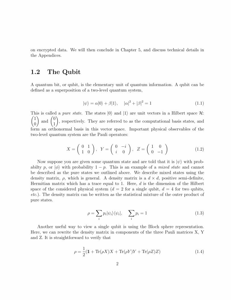
A quantum bit, or qubit, is the elementary unit of quantum information. A qubit can bedefined as a superposition of a two-level quantum system,

|ψ〉 = α|0〉+ β|1〉, |α|2 + |β|2 = 1 (1.1)

This is called a pure state. The states |0〉 and |1〉 are unit vectors in a Hilbert space H:(10

)and

(01

), respectively. They are referred to as the computational basis states, and

form an orthonormal basis in this vector space. Important physical observables of thetwo-level quantum system are the Pauli operators:

X =

(0 11 0

), Y =

(0 −ii 0

), Z =

(1 00 −1

)(1.2)

Now suppose you are given some quantum state and are told that it is |ψ〉 with prob-abilty p, or |φ〉 with probability 1 − p. This is an example of a mixed state and cannotbe described as the pure states we outlined above. We describe mixed states using thedensity matrix, ρ, which is general. A density matrix is a d × d, positive semi-definite,Hermitian matrix which has a trace equal to 1. Here, d is the dimension of the Hilbertspace of the considered physical system (d = 2 for a single qubit, d = 4 for two qubits,etc.). The density matrix can be written as the statistical mixture of the outer product ofpure states.

ρ =∑i

pi|ψi〉〈ψi|,∑i

pi = 1 (1.3)

Another useful way to view a single qubit is using the Bloch sphere representation.Here, we can rewrite the density matrix in components of the three Pauli matrices X, Yand Z. It is straightforward to verify that

ρ =1

2(1 + Tr(ρX)X + Tr(ρY )Y + Tr(ρZ)Z) (1.4)

2

Figure 1.1: The Bloch sphere has axes which correspond to the Pauli matrices, with theireigenstates at the poles. Single qubit states are vectors in the unit sphere, with pure statevectors (black) reaching the surface of the sphere, and mixed state vectors (blue) havingmagnitude < 1.

Now consider a space where the basis is the set of Pauli matrices. It can be shown thateach Pauli matrix is orthogonal to every other under the Hilbert-Schmidt inner product,(A,B) ≡ Tr(A†B). Then multiplying ρ by a Pauli matrix and taking the trace gives usthe projection of ρ onto one of the axes. In this way we can define a vector in our spaceof Pauli matrices which completely represents the quantum state. Fig. 1.1 shows a thestate vector on a Bloch sphere. The surface of the Bloch sphere contains the pure states,whereas mixed states fill the volume. The sphere then represents the set of states availablethrough single-qubit quantum processes.

Note that in this thesis we are concerned with quantum information encoded in thepolarization of single photons. We associate |0〉 with |H〉 (horizontal) and |1〉 with |V 〉(vertical), the linear polarizations of light. The reader should then be put on notice thatthe terms qubit and photon may be often used interchangeably.

1.3 Entanglement

Quantum entanglement is the greatest mark of the departure between quantum and clas-sical views of the physical world. It was with entanglement that John Bell showed how we

3

must leave behind our traditional notion of locality [9], and it is with entanglement thatquantum computers will provide dramatic increases in power over their classical counter-parts.

We will define entanglement using two qubits, though the concept extends to arbitrarydimensions. Simply put, two particles are entangled if they are not separable. To properlydefine separability of states, and therefore entanglement, we must consider mixed states.Suppose ρA and ρB are density matrices describing the quantum states of the particles Aand B. The particles are separable if the total quantum state ρ can be written as a convexsum of separable states

ρ =∑i

piρAi ⊗ ρBi (1.5)

where ⊗ is the tensor product,∑

i pi = 1 and each pi > 0. Once again, if the state cannotbe written in this way then it is entangled.

For example consider two particles, A and B, in the Bell state |Φ〉 = 1√2(|0A〉 ⊗ |0B〉+

|1A〉⊗|1B〉). Since it is not possible to factor the state into the form |Φ〉 = |ψA〉⊗|ψB〉, thestate |Φ〉 is entangled. Even if they are separated spatially, we can only think of the particlesas a single quantum system and not individually. We will come across entangled photonpairs numerous times. In Chapter 2, we will briefly discuss the generation of entangledphoton pairs, and in Chapter 3 we will use entangled photon pairs to characterize a singlequbit quantum channels.

1.4 Quantum channels

A quantum channel, or process, describes the most general evolution of a quantum statein time and/or space. Quantum channels can include anything from the quantum gatesthat make up a quantum computer, to the noisy and imperfect transmission of quantuminformation from one party to another. Formally, a quantum channel can be definedas a completely positive and trace-preserving linear map. Essentially, this means thata quantum channel is mapping that takes a physical density matrix to another physicaldensity matrix. The condition of complete positivity requires that the mapping takesdensity matrices to density matrices when including an arbitrarily large ancilla space. Inorder to better understand some of the work later on, particularly Chapter 3, it will beuseful to spend some time looking at some of the different representations of quantumchannels.

4

1.4.1 Kraus representation

One way to represent a quantum channel, E(ρ) is to describe the mapping as a sum oflinear operators, called Kraus operators, which individually act from the left and right onthe original density matrix ρ. For this reason it is also commonly called the operator sumrepresentation. The quantum state after the quantum channel, ρ′, is then

ρ′ = E(ρ) =∑i

AiρA†i (1.6)

where {Ai} are the Kraus operators and have the condition that∑

iA†iAi = 1. The amount

of Kraus operators required for the channel depends on the process, up to a maximum ofd2 operators [52].

The most important quantum gates are unitary operations, meaning that if U is aunitary operation then UU † = U †U = 1. Quantum gates are then, as a consequence,unital processes, meaning that they map the maximally-mixed state, ρ = 1/d, to itself.Quantum gates require only one Kraus operator to describe the quantum process. Anexample of a single-qubit quantum gate is the Hadamard which can be written as the sumof Pauli X and Z operators, H = (X + Z)/

√2.

A non-unital channel is a process which does not preserve the maximally-mixed state.An important example of this, and one which we will come back to in Chapter 3, is theamplitude damping channel, which has Kraus operators

A1 =

(1 00√

1− γ

), A2 =

(0√γ

0 0

), (1.7)

The channel models, for example, the excited state of the two-level system decaying to theground, and so γ represents the decay rate.

An example of a single-qubit quantum channel which requires all four Kraus operatorsis the completely depolarizing channel, which maps every input state to the maximally-mixed state. Its Kraus operators are given by the identity and the three Pauli operators,X, Y and Z. We will encounter the depolarizing channel more in Chapter 4 when we lookat how to hide quantum states and operations from an eavesdropper.

5

1.4.2 Superoperator representation

Another common way to represent a quantum channel is using a superoperator, a d2 ×d2 matrix which is commonly written in the basis of Pauli matrices. We will see thisrepresentation much more when we discuss quantum process tomography. We will beusing the terms superoperator, process matrix, and χ matrix interchangebly. The processmatrix shares many properties with a density matrix. For instance, the process matrix isboth Hermitian and positive semi-definite. The superoperator representation is also veryconvenient since for the single-qubit it gives the direct description of how a state’s Blochsphere coordinates change under the action of the channel. The superoperator can bederived simply from the Kraus operator representation by rewriting each Kraus operatorin the basis of Pauli matrices.

E(ρ) =∑i

AiρA†i

=∑i

(∑m

eimEm

)ρ

(∑n

e∗inE†

)=

∑mn

χmnEmρE†n (1.8)

where χmn =∑

i eime∗in. As an example, the process matrix for the amplitude damping

channel of Eq. 1.7 is shown below.

χAD =

14

(1 +√

1− γ)2

0 0 γ4

0 γ4− iγ

40

0 iγ4

γ4

0γ4

0 0 14

(−1 +

√1− γ

)2

(1.9)

where the basis is {1, X, Y, Z}. Fig. 1.2 shows the action of the amplitude damping channelon the Bloch sphere as the amount of damping increases.

1.4.3 Choi matrix representation

The final representation of a quantum channel we will discuss is the Choi matrix. In thesingle qubit case, the Choi matrix is a two-qubit density matrix describing the resulting

6

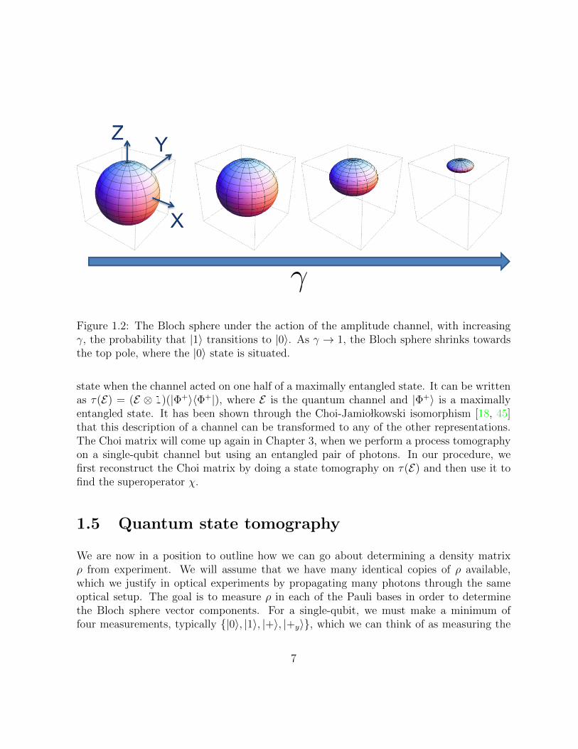
Figure 1.2: The Bloch sphere under the action of the amplitude channel, with increasingγ, the probability that |1〉 transitions to |0〉. As γ → 1, the Bloch sphere shrinks towardsthe top pole, where the |0〉 state is situated.

state when the channel acted on one half of a maximally entangled state. It can be writtenas τ(E) = (E ⊗ 1)(|Φ+〉〈Φ+|), where E is the quantum channel and |Φ+〉 is a maximallyentangled state. It has been shown through the Choi-Jamio lkowski isomorphism [18, 45]that this description of a channel can be transformed to any of the other representations.The Choi matrix will come up again in Chapter 3, when we perform a process tomographyon a single-qubit channel but using an entangled pair of photons. In our procedure, wefirst reconstruct the Choi matrix by doing a state tomography on τ(E) and then use it tofind the superoperator χ.

1.5 Quantum state tomography

We are now in a position to outline how we can go about determining a density matrixρ from experiment. We will assume that we have many identical copies of ρ available,which we justify in optical experiments by propagating many photons through the sameoptical setup. The goal is to measure ρ in each of the Pauli bases in order to determinethe Bloch sphere vector components. For a single-qubit, we must make a minimum offour measurements, typically {|0〉, |1〉, |+〉, |+y〉}, which we can think of as measuring the

7

projection onto each axis of the state vector on the Bloch sphere We need to measureboth eigenstates in one of the bases in order to properly normalize the state. Using singlephotons as an example, we would need to measure in both |0〉 and |1〉 in order to knowmany detectable photons, N , are incident on the measurement apparatus. Knowing N wecan then convert our measurements, which are numbers of photons, into probabilities anddetermine the projections onto each of the Bloch sphere axes. In actuality, we perform anovercomplete tomography, meaning that we measure each eigenstate for each of the Paulibases. This has been shown to give more accurate results, since the amount of photonspropagating through the setup can fluctuate over the time of measurement, skewing thenormalization.

1.5.1 Maximum likelihood

Nielson and Chuang [52] describe a method to reconstruct the density matrix from exper-imental results using a linear inversion. However, following [40] we will, in later chapters,perform maximum likelihood estimations of density matrices. A density matrix ρ(~t) canbe parametrized using d2− 1 independent real numbers thanks to normalization. For easeof calculation we normally use d2 numbers for the parametrization: ~t = {t1, t2, ..., td2}.This is done by first defining a lower triangular matrix T , which for the single-qubit caseis given by

T =

(t1 0

t3 + it4 t2

)(1.10)

It can be shown that ρ = T †T/Tr(T †T ) has all the properties required for a physicaldensity matrix, for single-qubit or higher dimensional cases. We define ni as the actualmeasured counts, and ni = N〈ψi|ρ(~t)|ψi〉 as the expected counts, given the density matrixρ(~t), measurement basis |ψi〉, and N photons incident on the detectors. We assume thatmeasured counts follow a Poissonian distribution, and so we make the approximation thatthe standard deviation in the measured counts σi ≈

√ni. When N is large, the Poissonian

distribution is approximately Gaussian. We can then calculate the probability of receivingthe measured counts in all k bases, assuming that the probability of measuring ni countsfollows a Gaussian distribution centred around ni.

P (n1, n2, ..., nk) =1

Nnorm

k∏i=1

exp

[−(ni − ni(~t))2

2σ2i

](1.11)

8

where NNorm is a normalization constant and σi is the standard deviation in the ith mea-surement. Substituting in ni for the standard deviation, we obtain the likelihood that ρ(~t)produced the measured counts

P (n1, n2, ..., nk) =1

Nnorm

k∏i=1

exp

[−(ni −N〈ψi|ρ(~t)|ψi〉)2

2N〈ψi|ρ(~t)|ψi〉

](1.12)

As the name of the technique suggests, we want to find the parameters ~t which maximizethis likelihood. Instead of maximizing P , it is an equivalent problem to maximize thelogarithm of P , which is also equivalent to minimizing the following “likelihood” function:

L(~t) =k∑i

[ni −N〈ψi|ρ(~t)|ψi〉

]22N〈ψi|ρ(~t)|ψi〉

(1.13)

Minimizing this function over ~t gives the density matrix which most closely represents theactual quantum state in the experiment. In this thesis, restructed density matrices arefound using the NMinimize function in Wolfram Mathematica 8.0.

1.5.2 Monte Carlo error analysis

The question arises of how to perform uncertainty analysis for the reconstructed densitymatrix. The method which is often used [53, 62], and which we also adopt for the work inthis thesis, is to add Poissonian noise to the measured photons counts. We then performmany reconstructions of the density matrix from the adjusted counts in a Monte Carlofashion, and can find the standard deviation of each density matrix element, or whichevermeasure desired. In order to analyze uncertainties in this way, we must make the assump-tion that the original number of photon counts measured is close to the mean, so that weare justified in adding statistical noise in this manner. By counting photons for long timesand accumlating many counts we reduce the fractional error, which goes as 1/

√ni.

1.6 Quantum process tomography

Characterizing quantum processes is of grave importance to implementing quantum tech-nologies. In order to see how close to the ideal implemented gates function, we must

9

perform a quantum process tomography. Since we are aiming to reconstruct the processmatrix χ, which shares all the same properties as a density matrix, we can take somelessons from quantum state tomography. We must still measure an input state in each ofa complete set of bases, but now we must also prepare and send in a complete set of inputstates.

In total, the χ matrix for a process acting on a d-dimensional Hilbert space is describedby d4 − d2 real parameters. We can see where the d4 amount comes from using theproperty that a Hermitian matrix cans be constructed using a single triangular matrix andits adjoint. Explicitly, if T is a lower triangular matrix then TT † is a Hermitian matrix.A triangular matrix, where diagonal elements are constrained to be real, is desribed by atotal of d4 real parameters. Adding the constraint that a process matrix must be tracepreserving leaves us with d4 − d2 real parameters to describe χ [52].

1.6.1 Maximum likelihood

In [52], a method for performing quantum process tomography is outlined using a linearinversion. As in state tomography, the issue arises in this technique where the linearinversion may output a χ matrix that has trace of greater than one, and therefore cannotbe a physical mapping. For this reason we turn to a maximum likelihood technique, as forthe quantum state tomography, and search for the physical χ matrix which most closelydescribes the observed measurement results. Following the same logic as the appendixof [19], we will denote nab as the number of measured counts for the ath input state andbth measurement setting. We can then define the number of expected counts that areoutput from the quantum channel as nab. Since we can write the action of the channelacting on an input state ρa as E(ρa) =

∑mn χmnEmρaE

†n, the expected counts are nab =

NTr(|ψb〉〈ψb|E(ρa)). We define the likelihood function L in the same way as for statetomography, with one addition. We add a Lagrange multiplier term λ to enforce physicalcontraints of the χ matrix. Recall that for a physical channel, we require that the Krausoperators {Ei} have the relation

∑iE†iEi =

∑mn χmnE

†nEm = 1. Multiplying both sides

by Ek and taking the trace, we can see that∑

mn χmnTr(E†nEmEk)−Tr(Ek) = 0, where kruns from 1 to d2. The likelihood function we seek to minimize takes the form

L =∑

ab

[nab−N∑

mn χmnTr(|ψb〉〈ψb|EmρaE†n)]

2

2N∑

mn χmnTr(|ψb〉〈ψb|EmρaE†n)

+ λ∑

k

(∑mn χmnTr(E†nEmEk)− Tr(Ek)

)2

(1.14)

10

1.6.2 Ancilla-assisted process tomography

So far we have discussed process tomography where we must input at least d2 to thequantum channel, and perform d2 measurements on each. For a single-qubit quantumchannel, this makes 4 measurements on 4 input states. Using a second, ancilla, qubit wecan shift the work from both preparing and measuring states, to only measurement. Bypreparing a two-qubit state, ρAB, and sending one qubit through the quantum channel(E ⊗ 1)(ρAB), reconstructing the process E requires just d4 = 16 measurements on thisjoint state. We can then perform a maximum likelihood estimation of the process matrixin the same way as outlined above, only now there is one input state and we only sumover measurement settings. It is not necessary for the characterization, but it has beenshown that having entanglement between the two qubits of the input state gives betterdefined results [3]. Using a maximally entangled input state, one actually can perform astate tomography on the output state from the channel, obtaining the Choi matrix for theprocess. We will use this in Chapter 3, adapting the technique according to the reality ofhaving imperfect resources states to input to the channel.

1.6.3 Monte Carlo error analysis

The uncertainty analysis for the reconstructed process matrix follows the same logic as forthe density matrix in the above section. We add Poissonian noise to the measured countsand perform many process tomography reconstructions. We then get an estimate of theuncertainty in the χ matrix, and figures of merit such as the process fidelity, which wediscuss in the next section.

1.7 Distance measures

In both Chapters 3 and 4, we will measure quantum states and processes. In order tocompare experimental findings to what is expected, it will be useful for us to lay out somequantitative ways [29] to distinguish between ideal and actual quantum states, or processes.

1.7.1 State fidelity

Defined by Jozsa in [41], the measure of the fidelity between two quantum states followsthe same intuition as the overlap between two states |ψ〉 and |φ〉, but generalized to mixedstates. For two states ρ and σ the quantum state fidelity is defined as

11

F (ρ, σ) =

(Tr√√

ρσ√ρ

)2

(1.15)

It can be seen that F = 1 when ρ and σ are equal, and that F = 0 when ρ and σ areorthogonal states. This measure is useful because more often than not, we are wantingto compare an experimentally found density matrix ρ against some pure state |ψ〉. Thefidelity then simplifes as

F (|ψ〉, ρ) =(

Tr√〈ψ|ρ|ψ〉 · |ψ〉〈ψ|

)2

(1.16)

= 〈ψ|ρ|ψ〉 (1.17)

which is the overlap between |ψ〉 and ρ.

1.7.2 Process fidelity

The process fidelity is a distance measure between two quantum processes. It is defined as

F (χ1, χ2) =

(Tr√√

χ1χ2√χ1

)2

(1.18)

This measure is often quoted against an ideal case when trying to implement a quantumgate. Similar to the state fidelity, when comparing against a unital channel, the fidelitysimplifies to the overlap of the χ matrices. However, if we are looking at an implementationof a non-unital channel, as we will in Chapter 3, the process fidelity lacks this operationalmeaning when comparing experimental and ideal cases. For this we must turn to anotherdistance measure.

1.7.3 Trace distance

The trace distance between two quantum states ρ and σ is defined as

D(ρ, σ) =1

dTr |ρ− σ| , (1.19)

12

where d is the dimension of the Hlibert space (d = 2 for a single qubit), and |M | =√M †M .

Note that here D = 0 when the states ρ and σ are equal, and has a maximum of D = 1when the states are orthogonal. We are interested in how to compare two quantum channelsEA and EB, so we look at the maximum trace distance measure. For this we input a state ρinto both channels and find the resulting states ρ′A = EA(ρ) and ρ′B = EB(ρ). Then we cantake the trace distance between ρ′A and ρ′B, which gives us a measure of the probabilityof distinguishing between the two states, and therefore the probability of distinguishingbetween the two channels for the state ρ. We then maximize this quantity over all possibleinput states ρ. Operationally, this means that we have found the highest probability oftelling the two channels apart using the best possible input state. At first glance, thismaximization problem seems daunting since even for a single-qubit channel, maximizingover the Bloch sphere volume is difficult. Thankfully, the state which maximizes the tracedistance will always be pure, reducing the computational problem dramatically.

13

Chapter 2

Quantum optics background

2.1 Introduction

In this chapter we will develop some of the quantum optics tools required to perform thetypes of experiments coming in later chapters. We will briefly overview concepts such asspontaneous parametric downconversion, entanglement generation, birefringence, Hong-Ou-Mandel interference and Pockels cells. Lastly, we will, in some detail, go through theexperimental setup for an optical CNOT gate.

We use the polarization of the light field to define our notion of information. Light canbe linearly, or circularly polarized (Fig. 2.1). We use the horizontal polarization (|H〉),defined as being in the plane of the optical table, as the logical state |0〉. The verticalpolarization, |V 〉, is the logical |1〉.

Then the diagonal polarization, |D〉, is |+〉 = 1√2(|0〉 + |1〉), and the anti-diagonal

polarization, |A〉, is |−〉 = 1√2(|0〉− |1〉). These are the eigenstates of the Pauli X operator.

Lastly, the left-circular polarization, |L〉, is |+y〉 = 1√2(|0〉 + i|1〉), and the right-circular

polarization, |R〉, is |−y〉 = 1√2(|0〉−i|1〉). These are the eigenstates of the Pauli Y operator.

Of course, nothing about this information encoding is quantum yet. Polarization opticsusing a matrix algebra formulation, such as Jones matrices or the Poincare sphere, datesback well before the Bloch sphere was used to described spin orientations.

14

z

y

x

z

y

x

a b

Figure 2.1: Linearly (a) and circularly (b) polarized light propagating in the z-direction.Blue arrows show the direction of the electric field at each point along the z-axis.

2.2 Generation of single photon entangled states

For the work presented in this thesis, we produce single photon states through a nonlinearoptical process called spontaneous parametric downconversion (SPDC). Simply put, SPDCis a process whereby an incoming pump photon “splits” into two photons of lower energies,called the signal and idler (Fig.2.2a).

2.2.1 Spontaneous parametric downconversion

SPDC occurs in a nonlinear medium, meaning there is a nonlinear response of the medium’selectric field to the electric field of the propagating light. The strength of this nonlinearityis given by the susceptiblity tensor ~χ. This is expressed through the polarization of themedium [12], P (t) = ε0

[χ(1)E(t) + χ(2)E2(t) + ...

]. Here we only consider nonlinear effects

due to the χ(2) term. For the two experiments in this thesis we use potassium titanyl phos-phate (KTP), and barium borate (BBO), materials with χ(2) nonlinearities large enoughto be used for efficient downconversion.

SPDC is a quantum effect that the classical nonlinear optics theory does not accountfor. Classically, we would describe the process of downconversion as a three-wave mixing[51]. For this discussion, we will assume that the input field, called the pump, and twooutput fields, traditionally called signal and idler, are all plane waves travelling along thez-axis. Each field is then given by an electric field operator E

(+)j = Ejei(kjz−ωjt), where Ej

is the field amplitude and ωj is its frequency. For signal, idler and pump field amplitiudesEs, Ei, and Ep, the respective coupled field equations for three-wave mixing in a χ(2) mediumare:

15

dEsdz

∝ χ(2)E∗i Epe−i∆kz (2.1)

dEidz

∝ χ(2)E∗sEpe−i∆kz (2.2)

dEpdz

∝ χ(2)EsEiei∆kz (2.3)

where ∆k is the phase mismatch defined as ∆k = kp − ks − ki, and z is the distance alongthe medium which in this case is a non-linear crystal. Now, for downconversion we initiallyonly have amplitude in the pump field E3, and E1 = E2 = 0. From the equations above, wehave that all three derivatives are equal to zero, and so no intensity can build up in thesignal and idler modes over the length of the crystal. It is for this reason that we must turnto a quantum mechanical description of downconversion. The interaction Hamiltonian is[36]

Hint = −ε03χ(2)

∫V

dV E(+)p E(−)

s E(−)i + E(−)

p E(+)s E

(+)i (2.4)

where ε0 is the vacuum permittivity, V is the crystal volume in which the interaction istaking place. For the quantum process we must first quantize the electric fields, such thatthey describe single photon propagation. For simplicity, we will assume the three fieldsare all plane waves occupying single modes, and propagating in the positive z direction.Taking the signal and idler modes to be initially in the vacuum state, and the pump modeto be a coherent state |α〉, the state |ψ(t = 0)〉 = |α〉p|0〉s|0〉i evolves under the interactionHamiltonian as

|ψ(t)〉 = e−iHintt/~|α〉p|0〉s|0〉i

= |α〉p|0〉s|0〉i + iε0χ

(2)t

3~

∫ t

0

dt′∫V

dV E(+)p E(−)

s E(−)i |α〉p|0〉s|0〉i + ... (2.5)

where higher order terms will be heavily suppressed. Also, the second term in the interac-tion Hamiltonian, E

(−)p E

(+)s E

(+)i , will not contribute since the signal and idler modes are

initally in the vacuum. We will focus on the first-order term from here on, since it showsthe generation of single photons. We write quantized single-mode electric field operatorsas

16

E(+)j = i

√~ωj

2ε0Vaje

i(kjz−ωjt) (2.6)

where aj is the annihilation operator for the jth mode. We can rewrite the state evolutionand drop the constant prefactors:

|ψ(t)〉 =

(~

2ε0V

) 32 √

ωpωsωiε0χ(2)t

3~

∫ t

0dt′∫VdV apa

†sa†i e

i(kpz−ωpt′)−i(ksz−ωst

′)−i(kiz−ωit′)|α〉p|0〉s|0〉i

∝ t

∫ t

0dt′∫VdV αei(kp−ks−ki)ze−i(ωp−ωs−ωi)t

′|α〉p|1〉s|1〉i (2.7)

where single photons have been generated in the signal and idler modes. Since the timeinterval over which the interaction occurs is long compared to optical frequencies, we canmake the approximation that

limt→∞

∫ t

0

dt′e−i(ωp−ωs−ωi)t′= 2πδ(ωs + ωi − ωp) (2.8)

which shows that the process conserves energy, ωs + ωi = ωp. Next we must discuss theremaining spatial integration

∫VdV ei(kp−ks−ki)z. This integration can be performed if we

take the interaction volume to have sidelengths Lx, Ly, and Lz. It is clear to see that theintegral is maximized when the phase mismatch term ∆k = kp−ks−ki = 0. If we integrateover one direction, we can gain some intuition for how the strength of the interaction varieswhen δK 6= 0.

∫ Lz

0

dzei∆kzz =i

∆kz

(1− ei∆kzLz

)= ei∆kzLz/2(−i) 2i

∆kzsin

(∆kzLz

2

)= ei∆kzLz/2Lzsinc

(∆kzLz

2

)(2.9)

The phase mismatch then deviates from the ideal as a product of three sinc functions, onein each direction.

Before moving on to further discussing phase matching, we should note that if we hadkept the next-order term in the series expansion of e−iHintt/~ we would have found a term

17

b a c

optic axis

Figure 2.2: (a) A cartoon of the SPDC process in a material with a χ(2) nonlinearity.Energy is conserved in the process. (b) shows the absorption of a pump photon at fre-quency ωp and the spontaneous emission of signal and idler photons at frequencies ωs andωi. (c) shows the conservation of momentum between pump and downconverted photons.Angle tuning (changing θ) allows for variety in signal and idler momenta and wavelengths.Downconverted photons are emitted at angles φ and ϕ from the pump propagation (forco-linear phase matching these angles are both ≈ 0).

which describes two photons generated in the each mode. We call these “double pairs”and can be detrimental to experiments based off of postselecting on coincident photondetections, since they can trigger false counts. For this reason we often reduce the pumppower while performing experiments to observe higher fidelity quantum operations.

2.2.2 Phase matching

As stated above, ∆k = kp − ks − ki is the phase mismatch, which we want to minimize.This can be achieved by phase matching techniques such as angle tuning (Fig. 2.2c), as isthe case when using BBO, or temperature tuning for KTP. We also use a periodically-poledKTP crystal (PPKTP) to further compensate for the phase mismatch through quasi-phasematching. The idea behind periodic poling is that over the length of the KTP crystalthe pump phase oscillates (Fig.2.3a), reducing the downconversion efficiency. However,if after some characteristic length in the material, Λ/2, we flip the crystal’s orientation,the pump is brought back into phase (Fig.2.3b). Performing these flips, called periodicpoling, along the entire length of the crystal keeps the pump beam in phase, and allowsthe downconversion efficiency to continually increase. In practice, the orientation of thecrystal is periodically flipped on the micrometer scale by applying a strong electric field.

It is also necessary to quickly discuss the polarization of the downconverted photons.There are two types of phase matching, which will depend on the birefringence of the

18

z a b

crystal orientation

Figure 2.3: (a) Phasor diagram of the pump propagating through the crystal withoutquasi-phase matching. (b) With quasi-phase matching, the crystal orientation is flippedeach half cell, Λ/2, reversing the phase.

nonlinear material. Type I downconversion emits signal and idler photons with the samepolarization, which is opposite to that of the pump, |H〉p → |V 〉s|V 〉i. We use type I down-conversion with a BBO crystal for the experiment in Chapter 4. Type II downconversionemits signal and idler photons with opposite polarizations, |H〉p → |H〉s|V 〉i. We use typeII downconversion for the experiment in Chapter 3, along with an additional conditionthat the signal and idler photons are emitted collinearly (φ, ϕ ≈ 0 in Fig. 2.2c).

2.2.3 Polarization entanglement

In Chapter 3, we use a source of photons, entangled in polarization, to characterize aquantum channel. It is useful for us to review how these entangled states are generated.We use a Sagnac interferometer, shown in Fig. 2.4. The polarization of the pump is setusing a half- and quarter-wave plate (HWP and QWP). First suppose that the pumpis H-polarized. It will then propagate around the interferometer in the counterclockwisedirection. If it downconverts (type II colinear) in the PPKTP crystal, the resulting stateis |H〉s|V 〉i. The photons then pass through the HWP at 45◦, and are split into differentspatial modes by the polarizing beam splitter (PBS) giving the state |H〉1|V 〉2, wherethe subscripts refer to the spatial modes. Now suppose the pump is V-polarized. It thenpropagates clockwise around the interferometer, is flipped to horizontal polarization by theHWP, and then downconverts to |H〉s|V 〉i. The photons are separated into spatial modesby the PBS, but this time the resulting state is |V 〉1|H〉2. Finally, suppose the pumpis set to the diagonal polarization |D〉 = 1√

2(|H〉 + |V 〉). It then propagates around the

19

PPKTP

HWP

QWP

1

2 Dichroic mirror

Filter

PBS

45o

Figure 2.4: A PPKTP crystal placed in a Sagnac interferometer. By controlling thepolarization state of the blue pump beam, the downconverted two-photon state can betailored, and entanglement can be generated.

interferometer in both directions, such that if we detected a downconverted photon pair, wedo not know through which direction of the crystal the process occured, and consequentlywe have generated the entangled state 1√

2(|H1V2〉+ |V1H2〉).

2.3 The beamsplitter and Hong-Ou-Mandel interfer-

ence

The beamsplitter is of fundamental importance in quantum optics as it allows for interac-tion between different spatial modes. We describe a beamsplitter using ladder operatorsfor each mode, see Fig. 2.5a. The beamsplitter transforms the ladder operators based onits reflectance and transmittance. They transform as

a 7→ tc+ rd

b 7→ td− rc (2.10)

where r and t are complex numbers with the condition that |r|2 + |t|2 = 1. We alsocommonly use polarizing beamsplitters (PBS), which transmit H-polarized light, while

20

Coinc.  

a b

19.8 19.9 20.0 20.1 20.2 20.3

0

50

100

150

200

250

300

350

400

Coi

ncid

ence

s [/s

]Motor Position [mm]

Visibility = 97.3%

Figure 2.5: (a) A simple HOM inteferometer. A beamsplitter maps photons in input modesa and b to output modes c and d. Simultaneous detections of photons in both output modestriggers the coincidence logic. (b) Detected coincidence counts when changing the pathlength of input mode a. HOM interference occurs when the path lengths are matched, asshown by the dip.

reflecting V-polarized light. The beamsplitter is often used in describing different inter-ference effects in optics. It is at the heart of the Michelson and Hanbury-Brown-Twissinterferometers. In a later section, we will look at the implementation of a two-photonentangling gate, and so we will primarily be concerned with the Hong-Ou-Mandel (HOM)interferometer [37] (Fig. 2.5a). Photons enter the setup in modes a and b, described inthe number state basis as |ψin〉 = |1a, 1b〉 = a†b†|0, 0〉. Supposing that we have a 50:50beamsplitter (r = t = 1/

√2), the ladder operators a and b are mapped to c and d such

that

|ψout〉 =1√2

(c† + d†)1√2

(d† − c†)|0, 0〉

=1

2

((d†)2 − (c†)2

)|0, 0〉

=1√2

(|0c, 2d〉 − |2c, 0d〉) (2.11)

It can be seen that when the input photons arrive at the beamsplitter in the same timeand interference occurs, we get photon bunching, and have no coincidence photons between

21

modes c and d. If we record coincidence counts while varying one of the input photon pathlengths, we then observe the HOM dip (Fig. 2.5b). A more general treatment shows that toobserve interference photons must be indistinguishable in frequency, polarization, arrivaltime, and of course have overlap between output modes. We will discuss HOM interferenceagain shortly when we look at the implementation of an optical CNOT gate.

2.4 Pockels cells

Pockels cells are comprised of a non-linear crystal which is quickly switched between twoindices of refraction controlled by fast-switching high voltages. They are based off ofthe Pockels effect, where a strong electric field applied to a non-linear medium changesthe effective index of refraction. In linear optics these cells can be used for fast-unitaryoperations in feed forwards systems, or to perform one-time pads for encrypting photonicqubits, as we do in Chapter 4.

The Pockels cells are driven by square waves voltages oscillating between high and lowstates, which then control the oscillation between two amounts of effective bifringence,±λ/4. A quarter-wave plate immediately after each Pockels cell shifts these rotations to0 and λ/2, meaning that the Pockels cell either acts as the identity, or a half-wave plateat the angle of the crystal’s orientation. Half-waves plates before and after each Pockelscell are used to set the angle of the half-wave rotation about an arbitrary axis in the x-zplane of the Bloch sphere. The crystals in each Pockels cell are aligned at 45 + δ degreesto the plane of the optical table, where δ is small. For the experiment in Chapter 4, weuse three Pockels cells to perform X, Hadamard, and Phase gates. In order to perform anX rotation, half-wave plate at 45 degrees, the additional HWPs are both then set to δ/2degrees.

1 = HWP(θ = δ/2) ·QWP(θ = π/4 + δ) ·PC(φ = −λ/4, θ = π/4 + δ) · HWP(θ = δ/2),

X = HWP(θ = δ/2) ·QWP(θ = π/4 + δ) ·PC(φ = λ/4, θ = π/4 + δ) · HWP(θ = δ/2) (2.12)

where the Pockels cell (PC) is modeled as a general waveplate with retardance φ and opticaxis at angle θ. The second Pockels cell switches between performing the identity and theHadamard gate. Here we want the HWPs before and after the Pockels cell to be at 11.5±δdegrees, and so it can similarly be shown

22

1 = HWP(θ = 3π/16 + δ/2) ·QWP(θ = π/4 + δ) ·PC(φ = −λ/4, θ = π/4 + δ) · HWP(θ = 3π/16 + δ/2),

H = HWP(θ = 3π/16 + δ/2) ·QWP(θ = π/4 + δ) ·PC(φ = λ/4, θ = π/4 + δ) · HWP(θ = 3π/16 + δ/2) (2.13)

The last Pockels cell switches between performing the identity and the Phase gate(|0〉 7→ |0〉, |1〉 7→ i|1〉). Because this is a quarter-wave rotation, we oscillate the voltagebetween ±λ/8 and require an eighth-waveplate (EWP) afterwards, for which we can use ahalf-waveplate tilted to give the proper amount of birefringence. It is simple to verify that

1 = EWP(θ = 0) · HWP(θ = π/8 + δ/2) ·PC(φ = −λ/8, θ = π/4 + δ) · HWP(θ = π/8 + δ/2),

P = EWP(θ = 0) · HWP(θ = π/8 + δ/2) ·PC(φ = λ/8, θ = π/4 + δ) · HWP(θ = π/8 + δ/2) (2.14)

2.5 Optical CNOT gate

The controlled-NOT, or CNOT, gate is of critical importance to quantum computing, andis commonly used in the set of quantum gates required for universal computation [52]. Thematrix for the CNOT operation is

CNOT =

1 0 0 00 1 0 00 0 0 10 0 1 0

(2.15)

The importance of the CNOT can be seen in its ability to entangle two initially separablequbits. For example, suppose a two-qubit state is initialized as |+0〉, where |+〉 = 1√

2(|0〉+

|1〉), then the output state after applying a CNOT gate with the first qubit as the controlis

CNOT|+0〉 =1√2

(|00〉+ |11〉), (2.16)

23

which is the maximally entangled state. To build a CNOT using linear optics requires theinteraction of the two photonic qubits at some optical element. The scheme used for thisproject is shown in Fig. 2.6, and is derived from that shown in [42, 46, 53], which gives a gatesuccess probability of 1/9. Photons meet at a partially-polarizing beam splitter (PPBS),where H-polarized light is fully transmitted, and V-polarized light is 1/3 transmitted and2/3 reflected.

2.5.1 Partially-polarizing beamsplitters

Similar to the PBS we discussed earlier, the partially-polarizing beamsplitter (PPBS) per-forms the following mappings on the lowering operators:

aH → cH

aV →1√3cV +

√2

3dV

bH → dH

bV →1√3dV −

√2

3cV (2.17)

Now suppose two indistinguishable V-polarized photons arrive at the PPBS at the sametime, one in mode a and one in mode b. Then the PPBS maps

a†V b†V |00〉ab →

1

3(−c†V d

†V −√

2c†2V +√

2d†2V )|00〉cd (2.18)

When no interference occurs, the maximum probability of observing a coincident pho-

tons in each path is(

23

)2+(

13

)2= 5

9. In the coincidence subspace, detecting one photon

in each output mode, we see that the amplitude is 1/3 of the original, giving a reductionto a minimum of 1/9. The visibility of this HOM interference is calculated as follows,

Vis =Max−Min

Max

=5/9− 1/9

5/9

= 4/5 (2.19)

24

HWPs at 45 deg

PPBS: H is fully trans, V is 1/3 trans, 2/3 refl.

PBSs and WPs for state preparation

QWP to set phase

to tomography

to tomography

a

b

c

d

Hadamard: HWP at 22.5 deg

Batears set to do X

Polarization Analyzer

PPBS: H is fully trans, V is 1/3 trans, 2/3 refl.

a

b

Figure 2.6: (a) Photons of indistinguishable frequency in input modes a and b interfereat the first PPBS. Polarizations are flipped using half-wave plates at 45 degrees. A tiltedquarter-wave plate in one mode compensates for unwanted phases due to mismatched pathlengths. Two further PPBSs normalize the output state in modes c and d. Post-selectingon coincidences in the c and d modes gives the desired output state with 1/3 of the originalamplitude. (b) Additional Hadamard and Pauli X components transform the setup intoa CNOT gate. State preparation and analysis are performed using a PBS, quarter- andhalf-wave plate, and photons detected within a 3 ns window are recorded.

25

1 9 . 4 1 9 . 6 1 9 . 8 2 0 . 0 2 0 . 2 2 0 . 4 2 0 . 62 0 04 0 06 0 08 0 0

1 0 0 01 2 0 01 4 0 01 6 0 01 8 0 02 0 0 02 2 0 0

Coinc

idenc

es [/s

]

M o t o r P o s i t i o n [ m m ]

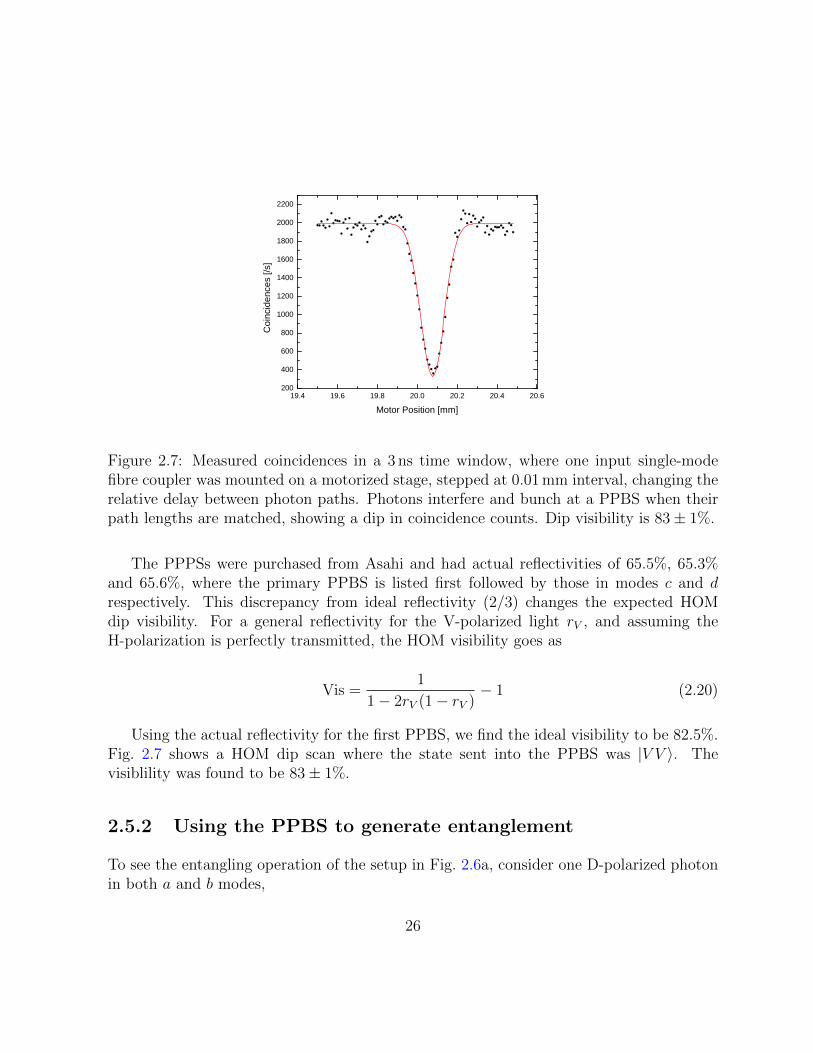
Figure 2.7: Measured coincidences in a 3 ns time window, where one input single-modefibre coupler was mounted on a motorized stage, stepped at 0.01 mm interval, changing therelative delay between photon paths. Photons interfere and bunch at a PPBS when theirpath lengths are matched, showing a dip in coincidence counts. Dip visibility is 83± 1%.

The PPPSs were purchased from Asahi and had actual reflectivities of 65.5%, 65.3%and 65.6%, where the primary PPBS is listed first followed by those in modes c and drespectively. This discrepancy from ideal reflectivity (2/3) changes the expected HOMdip visibility. For a general reflectivity for the V-polarized light rV , and assuming theH-polarization is perfectly transmitted, the HOM visibility goes as

Vis =1

1− 2rV (1− rV )− 1 (2.20)

Using the actual reflectivity for the first PPBS, we find the ideal visibility to be 82.5%.Fig. 2.7 shows a HOM dip scan where the state sent into the PPBS was |V V 〉. Thevisiblility was found to be 83± 1%.

2.5.2 Using the PPBS to generate entanglement

To see the entangling operation of the setup in Fig. 2.6a, consider one D-polarized photonin both a and b modes,

26

|ψ〉 = |DD〉= a†Db

†D|00〉ab

=1√2

(a†H + a†V )1√2

(b†H + b†D)|00〉ab (2.21)

Performing the first PPBS mapping and simplifying by postselecting on the coincidencebasis, one photon in each of the c and d modes, we find

|ψ〉 → 1

2

(c†Hd

†H +

1√3c†Hd

†V +

1√3c†V d

†H −

1

3c†V d

†V

)|00〉cd (2.22)

Half-wave plates at 45 degrees then flip H and V polarizations, H ↔ V , and the state afterthe second set of PPBSs is

|ψ〉 → 1

3· 1

2

(c†V d

†V + c†V d

†H + c†Hd

†V − c

†Hd†H

)|00〉cd

=1

3· 1

2(−|HH〉+ |HV 〉+ |V H〉+ |V V 〉) (2.23)

which is an entangled state. The factor of 1/3 corresponds to the success probabilty of thegate (1/9), while the rest of the state amplitude is lost when we postselect on coincidencesin the two paths. However, the operation that the setup in Fig. 2.6a performs is not aCNOT. One can verify that its operation is given by the following matrix,

S =

0 0 0 −10 0 1 00 1 0 01 0 0 0

(2.24)

This can be easily transformed into the CNOT gate (Fig. 2.6b) using Hadamards andPauli X rotations. It is straightforward to see that

CNOT = (1⊗ H) · S · (X⊗ X) · (1⊗ H) (2.25)

27

Figure 2.8: The real (a) and imaginary (b) parts of a density matrix reconstructed using amaximum likelihood quantum state tomography. Here, the state |DH〉 was sent into theoptical setup. The resulting density matrix has quantum state fidelity of 0.893 with the|Φ+〉 Bell state.

2.5.3 Experimental setup

Photon pairs were generated by spontaneous parametric downconversion (SPDC) usinga Titanium Sapphire (Ti:Saph) laser pulsed at 80 MHz to pump a 1 mm Barium Borate(BBO) crystal at 395 nm producing downconverted photons at 790 nm. Photons werepropagated through the optical setup outlined in Fig. 2.6b, and were detected using siliconavalanche photo-diodes (PerkinElmer four-channel SPCM-AQ4C modules) and coincidencephotons were counted with a timing window of 3 ns using a 16 channel logic unit.

2.5.4 Results

Preparing the state |HD〉, we expect to get out the |Φ+〉 Bell state. Fig. B.1 shows thereconstructed two-qubit density measured from the output of the CNOT setup comparedwith the ideal. The quantum state fidelity was calculated to be 0.893 ± 0.004, wherethe uncertainty was found using a Monte Carlo simulation adding Poissonian noise to themeasured state tomography data.

In order to fully characterize the gate, an overcomplete process tomography was per-

28

formed, where each of the 36 two-qubit Pauli basis states were input to the setup andphoton coincidence counts were measured in all 36 bases. Detailed results of this areshown in Chapter 4. The process fidelity between the ideal and experimental processmatrices was found to be 0.869± 0.004.

29

Chapter 3

Optimal linear opticalimplementation of a single-qubitdamping channel

3.1 Notes and acknowledgements

In this chapter we describe the implementation and characterization of a quantum channelwhich can controllably add a given amount and type of noise to a qubit. We build onthe discussions of quantum channels and process tomography in Chapter 1, and use theentangled photon source outlined in Chapter 2. We show that the optical setup was realizedin an optimal way, maximizing the probabilty of success of the channel.

Notice: The contents of this chapter has been published in:

K. A. G. Fisher, R. Prevedel, R. Kaltenbaek and K. J. Resch, Optimal linear opticalimplementation of a single-qubit damping channel. New Journal of Physics, 14, 033016,2012.

Author contributions

KF and RP performed the experiment and analyzed the data.

RK designed the experiment.

KR contributed to the design and realization of the experiment.

30

KF took primary responsibility for writing the first draft. All authors contributed toediting for the final version.

3.2 Abstract

We experimentally demonstrate a single-qubit decohering quantum channel using linearoptics. We implement the channel, whose special cases include the familiar amplitude-damping channel and the bit-flip channel, using a single, static optical setup. Followinga recent theoretical result [M. Piani et al., Phys. Rev. A, 84, 032304 (2011)], we realizethe channel in an optimal way, maximizing the probability of success, i.e., the probabilityfor the photonic qubit to remain in its encoding. Using a two-photon entangled resource,we characterize the channel using ancilla-assisted process tomography and find averageprocess fidelities of 0.98 ± 0.01 and 0.976 ± 0.009 for amplitude-damping and the bit-flipcases, respectively.

3.3 Introduction

Time evolution in quantum mechanics converts a density matrix to another density matrix.This evolution is referred to as a quantum channel and can be described mathematicallyas a completely positive (CP) map [52]. Due to generality of the concept of quantumchannels, their use is ubiquitous in quantum information. For example, unitary quantumchannels are used in quantum computing to describe quantum gates. Non-unitary channels,on the other hand, describe the interaction of quantum states with an environment, andhave recently been connected to fundamental physical questions in quantum informationscience, such as channel capacity, superadditivity [69, 33] and bound entanglement [38].

Linear optics and single photons have several characteristics that make them an idealtestbed for quantum information. Single-qubit unitaries are easy to implement as, for po-larization encoded qubits, they only require waveplates. Photonic qubits also exhibit longdecoherence times, and spontaneous parametric downconversion allows the generation ofhigh-quality entangled states, which can be easily manipulated. However, certain opera-tions, such as the two-qubit CNOT-gate, are difficult in this architecture [50, 48], and canonly be implemented probabilistically [44, 59, 54].

Unfortunately, the ease of single-qubit operations does not extend to more generalCP maps. Some quantum channels, like the depolarizing single-qubit channel [52] can

31

be implemented with unit probability, but this is not the case in general. For instance,the amplitude-damping channel, a non-unital quantum process, has been implemented inlinear optics only with a limited success probability of 1/2 [58, 47]. In one experiment [2],the Kraus operators describing an amplitude-damping channel were implemented usinga Sagnac interferometer such that all photons were transmitted. However, because theoutputs from each Kraus operator were not coherently recombined on a beamsplitter, ournotion of the success probability of a quantum channel does not apply to this case.

Recently, it was shown by Piani et al. [56] that, any single-qubit quantum channelcould be implemented probabilistically using linear optics and postselection, i.e., similarto many two-qubit operations. Moreover, they derived an explicit formula for the optimalsuccess probability.

In the present work, we use this recent theoretical result to design and demonstrate alinear-optics-based implementation of a certain class of non-unital single-qubit quantumchannels called “damping channels”. The class of channels we focus on can be parametrizedby two real numbers: α and β. In the operator-sum representation, the channel’s actionon an arbitrary quantum state ρ can be written as E(ρ) =

∑iAiρA

†i , where the two Kraus

operators are [73]:

A0 =

(cosα 0

0 cos β

), A1 =

(0 sin β

sinα 0

)(3.1)

This channel is of great interest as its special cases include the amplitude-damping (α =0) and bit-flip (α = β) channels, both of which are common sources of error in otherimplementations of quantum information processing, such as ion traps. Furthermore, itbelongs to the small class of quantum channels for which the quantum capacity can bedirectly calculated via the coherent information [23].

Here, we experimentally realize this single-qubit damping quantum channel using linearoptics. We can use the setup to add controlled amounts of noise of various types to a singlequbit. The schematics of the experimental setup are shown in Figure 4.4. The key step inthe implementation of the channel is the splitting of the polarization encoded informationinto different spatial modes, which then allows for the manipulation of different logicalstates independently of one another. An arrangement of half-wave plates and liquid-crystalretarders allows us to probabilistically implement both Kraus operators within a single,static optical setup. We characterize the channel using an ancilla-assisted quantum processtomography method, and show the optimality of our optical setup, with our success ratesin the amplitude-damping case surpassing those of previous implementations [58, 47]. Inorder to characterize the action of the channel on entanglement we study the amount ofentanglement of photon pairs when one photon is sent through the channel.

32

3.4 Optimality of the implementation

Following Ref. [56], it can be shown that the probability of success for a specific Kraus

decomposition {Ai} is psucc({Ai}) =(∑

i ‖Ai‖2∞)−1

, where the norm ‖M‖∞ is the largestsingular value of the operator M . Maximizing over all possible Kraus decompositionsAi describing the channel allows one to achieve the optimal success probability popt

succ =maxAi

1∑i‖Ai‖2∞

. For our particular channel, if we assume that cos(α) ≥ cos(β), this yields:

poptsucc =

1

cos2 α + sin2 β(3.2)

In order to achieve poptsucc, each Kraus operator is implemented with individual proba-

bilities pAi= ‖Ai‖2

∞ · poptsucc. We find that the optimal probability of success is achieved for

pA0 = cos2 αcos2 α+sin2 β

and pA1 = sin2 βcos2 α+sin2 β

. We show experimentally that for various values ofα and β, which can be independently controlled in our experiment, we indeed achieve thisupper bound.

3.5 Ancilla-assisted process tomography

Quantum process tomography (QPT) allows one to experimentally reconstruct the super-operator describing an unknown physical process. Ancilla-assisted QPT (AAQPT) usesancillary qubits to facilitate and reduce the reconstruction procedure to quantum statemeasurements only; AAQPT has been applied assuming that the initial state is perfect[3]. AAQPT provides us with the physical matrix that best describes the action of theexperimentally channel and has been used to study various unitary quantum gates. How-ever, it has not yet been extended to the characterization of non-unital channels which weaddress in our work. Here we describe and use a maximum likelihood approach for AAQPTthat takes into account the imperfection of the input ancilla state (Maximum likelihoodmethods have been applied to standard quantum state and process tomography before[40, 53, 27, 39, 6, 49]). To our best knowledge, a maximum likelihood AAQPT techniquewhich includes errors in the state preparation has not been implemented previously.

The standard techniques for QPT and AAQPT are described in [52, 40, 53, 19] and[3], respectively. Below, we outline our method following their nomenclature. Consider atwo-qubit state, ρAB, whose density matrix is known; e.g., it might have been reconstructedusing quantum state tomography (QST). The quantum channel E acts on subsystem A,while subsystem B is unaffected. The transformed two-qubit state after the channel is

33

ρ′AB = (E ⊗ 1) (ρAB). Characterizing ρ′AB, e.g., by performing standard QST, allows forreconstruction of the quantum process using the Choi–Jamio lkowski isomorphism [18, 45].

The quantum process can be written as ρ′AB =∑d2−1

m,n=0 χmn(Em⊗1)ρAB(En⊗1)† where

{Ei} are operators which form a basis in the space of d×d matrices (d = 2 in our case). Itis common to use the basis formed by the Pauli matrices {1, X, Y, Z}. The d2-dimensionalprocess matrix χ then fully describes the quantum process. In our maximum-likelihoodtechnique, we parameterize χ by d4−d2 = 12 real numbers [40, 53, 27] and seek to minimizethe following function:

f =ν∑i=1

(ni −NTr[Miρ′AB])2

2NTr[Miρ′AB]+ λ

∑k

[∑m,n

χmnTr(E†nEmEk)− Tr(Ek)

]2

,

such that the resulting χ most closely resembles a physical quantum process. Here, i labelsthe measurement setting in the final QST, ν is the number of measurement settings, ni isthe number of two-fold coincidence counts recorded in the ith setting, N corresponds to thenumber of photons incident on the detectors, Mi is the projector of the ith measurement,and λ is a Lagrange multiplier used to force the resulting process matrix to be tracepreserving [19].

3.6 Experiment

We use the experimental setup shown in Figure 4.4 to implement the quantum channeldefined by the Kraus operators in Equation 3.1. Two 40 mm calcite beam displacers areused to construct an interferometer. Within these beam displacers, photons with horizontal(|H〉) and vertical (|V 〉) polarization are spatially displaced with respect to each other [54].Half-wave plates (HWPs) are used to set the amount of damping by allowing to adjust αand β in Equation 3.1. The relations between these parameters and the individual anglesa, b, c, d of the four HWPs are given by sin 4a = cosβ

cosα, b = a − π

4, sin 4c = − sinα

sinβand

d = π2− c. The channel is realized by switching randomly between the Kraus operators A0

and A1. The switching is performed using two liquid-crystal retarders (LCRs). We set thetwo LCRs to X1 and 12, respectively, to implement A0, and we set them to 11 and X2 toimplement A1. Here, the subscripts represent the action of the first and the second LCR.The probabilities, pA0 and pA1 , with which each configuration is realized are determinedby the values of α and β such that the overall success probability of realizing the channel

34

Figure 3.1: The experimental setup. We use spontaneous parametric downconversion inperiodically poled KTiOPO4 (PPKTP) to generate entangled photon pairs of the form|Φ+〉 = 1√

2(|HH〉+ |V V 〉) which are subsequently coupled into single-mode fibres. One of

the photons is sent through the damping channel parameterized by α and β, which are setby the angles a, b, c and d of four half-wave plates (HWPs). Two liquid-crystal retarders(LCRs) switch anti-correlatively between the identity, 1, and the Pauli X operation. Thepolarization of each photon is measured by an analyzer (A and B) consisting of a half- anda quarter-wave plate (QWPs) followed by a polarizing beam splitter (PBS). Eventually,the photons are detected by single-photon counting modules.

35

follows Equation 3.2, and is optimal [56]. The switching rate of the LCRs was chosen tobe 10 Hz, significantly faster than the integration time for a single measurement (5 s).

To characterize the channel, we use the AAQPT scheme outlined above. Our resourcestate is an entangled photon pair generated in a type-II downconversion source in a Sagnacconfiguration [24, 57]. A 0.5 mW laser diode at 404.5 nm pumps a 25 mm periodically-poledcrystal of KTiOPO4 (PPKTP). This typically yielded a coincidence rate of 10 kHz. Thecharacterization of the channel is executed as follows: The HWP angles a, b, c and d areset to zero and the LCRs to X1 and 12 such that the channel acts as the identity map. AQST is performed to obtain the density matrix of the input state, ρAB. The HWP anglesand the probabilities for switching the LCRs and the HWP angles are then set according tothe values of α and β. Another QST yields the output state, ρ′AB. QST involves recordingcoincidences for all combinations of the eigenstates of the Pauli X, Y and Z operators.For each of these 36 projective measurements, we integrated coincidence counts for 5 s.The resulting data were then used in conjunction with Equation 3.3 to reconstruct thesuperoperator describing the quantum process.

3.7 Results

We now turn to our main result, the optimality of our quantum channel implementation.Figure 3.2a shows the probability of success for the amplitude-damping, bit-flip, and onein-between case (α = 2

3β). Since amplitude-damping manifests itself as photon loss in our

particular implementation, determining the probability of success reduces to measuringthe transmission of the channel. The experimental data closely follow the theoreticalpredictions (solid lines) that are based on Equation 3.2.

Previous optical implementations of the amplitude-damping channel [58, 47] have givenat most 50% probability of success, whereas here we find that only in the case of maximumdamping (β = π/2) the probability of success decreases to 50%. The experimental resultsfor the success probability closely resemble the theoretical prediction. This is also true forour experimental implementation of the bit-flip channel and the α = 2

3β case of single-qubit

damping.

Fig. 3.2b shows the tangle [74] of the two-photon output density matrix, ρ′AB, for theamplitude-damping, bit-flip, and α = 2

3β cases, where one of the two photons passes

through the quantum channel. Theoretical curves are based on the action of the respectiveideal quantum channels on the experimental input density matrix when the channel isturned off. This also explains the rather high deviation of the data points at larger values

36

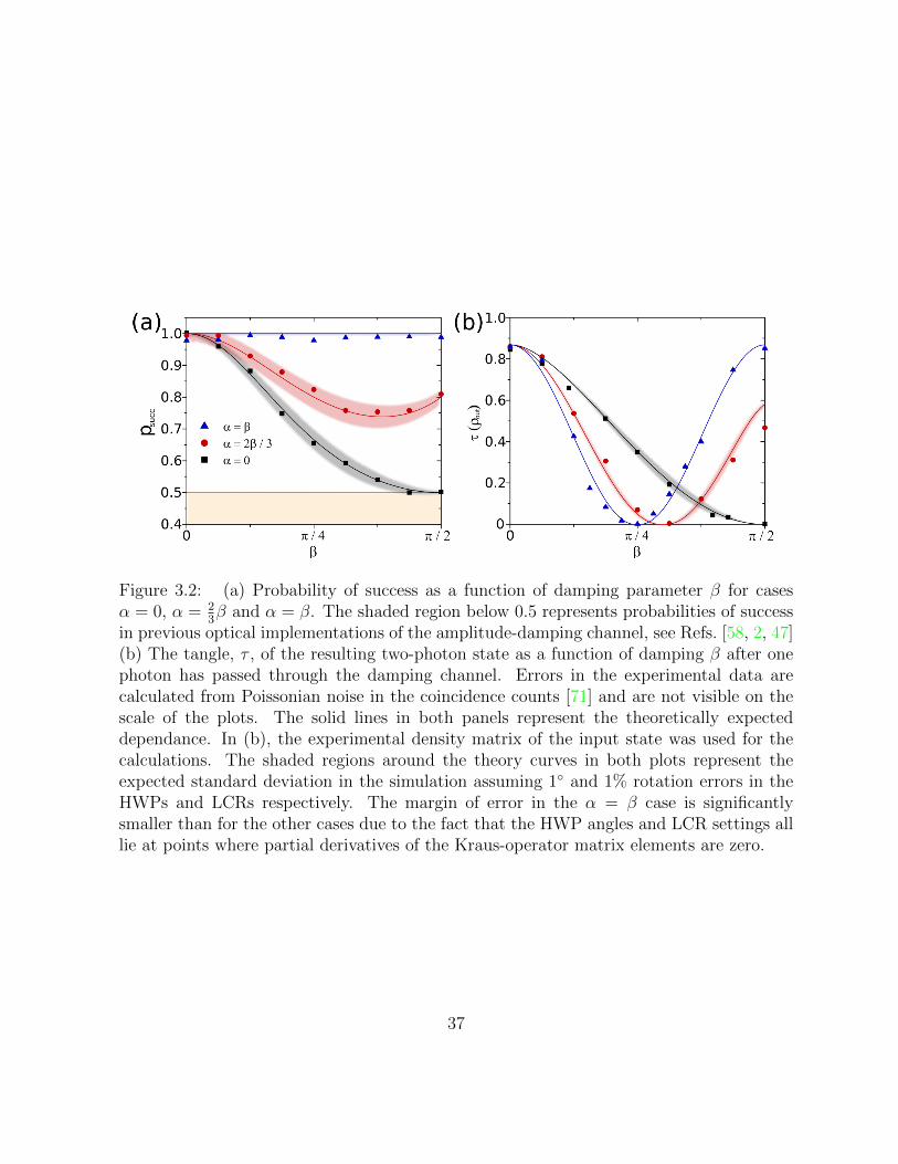
Figure 3.2: (a) Probability of success as a function of damping parameter β for casesα = 0, α = 2

3β and α = β. The shaded region below 0.5 represents probabilities of success

in previous optical implementations of the amplitude-damping channel, see Refs. [58, 2, 47](b) The tangle, τ , of the resulting two-photon state as a function of damping β after onephoton has passed through the damping channel. Errors in the experimental data arecalculated from Poissonian noise in the coincidence counts [71] and are not visible on thescale of the plots. The solid lines in both panels represent the theoretically expecteddependance. In (b), the experimental density matrix of the input state was used for thecalculations. The shaded regions around the theory curves in both plots represent theexpected standard deviation in the simulation assuming 1◦ and 1% rotation errors in theHWPs and LCRs respectively. The margin of error in the α = β case is significantlysmaller than for the other cases due to the fact that the HWP angles and LCR settings alllie at points where partial derivatives of the Kraus-operator matrix elements are zero.

37

Im( exp)

Re( exp)

Im( id)

Re( id)

00.8

0.85

0.9

0.95

1

Pro

cess F

idelity

0

0.1

0.2

0.3

0.4

0.5

Trace D

ista

nce

(a) (b)

Figure 3.3: (a) Measured process fidelity (solid data points) and trace distance (unfilleddata points) as a function of damping for each of the three cases studied. Error bars (∼10−3), calculated using Monte-Carlo simulations adding Poissonian noise to the measuredstate tomography counts in each run, are too small to see on this scale due to high photoncounting rates. Additional systematic errors are discussed in the text. (b) Real andimaginary parts of the experimentally determined and ideal process matrices at maximumamplitude-damping (α = 0, β = π/2).

of β, as drift in the optical setup can lead to slightly different input states over the courseof the experiment.

The process fidelity is defined by F =(Tr√√

χexpχid√χexp

)2[41], where χexp and χid

are the experimental and ideal process matrices, respectively. Process fidelities for the threetested cases, α = 0, α = β and α = 2

3β can be seen in Figure 3.3. The uncertainty in the

process fidelity of each individual point was estimated by maximum-likelihood assumingPoissonian noise in the measured counts and is on the order of 10−3. However, it is clearfrom the deviation of process fidelities over the range of damping values that there is anadditional systematic error. We attribute this systematic error to the reduced couplingefficiencies when rotating the half-wave plates in the interferometer when setting values ofα and β. We then estimate the statistical error in the data and find the average processfidelities to be 0.98± 0.01, 0.976± 0.009, 0.981± 0.004 for the three respective cases.

We also compute the maximum trace distance [52], which is defined asD = maxρin12Tr∣∣ρexp

out − ρidout

∣∣,where |A| =

√A†A and ρ

exp/idout =

∑m,n χ

exp/idmn EmρinE

†n. Operationally, D corresponds to

the highest probability of distinguishing between the experimental and ideal channels usingthe best possible input state. Maximum trace distances for α = 0, α = β and α = 2

3β

38

cases can also be seen in Figure 3.3. As with the process fidelities, we can estimate theerrors for the three cases from the statistical error of the data points for different valuesof β. Using this approach, the average maximum trace distances for α = 0, α = β, andα = 2

3β are 0.10± 0.01, 0.11± 0.02, and 0.11± 0.03, respectively.

3.8 Summary

Decoherence plays an important role in quantum information science. Investigating itseffects requires careful and well-controlled implementations of these noisy processes. Non-unital damping channels, like the ones studied here, are crucial in further understand-ing quantum communication, in determining channel capacities and for the generation ofbound-entangled states. We have implemented a general damping single-qubit quantumchannel with linear optics in which both type and amount of decohering noise can beprecisely controlled. A single, static optical setup can perform as the amplitude-dampingchannel, the bit-flip channel, or more general cases characterized by two real parameters,α and β. Most importantly, we have shown that this channel has been implemented in anoptimal way, so as to maximize the probability of success. The channels were characterizedusing a new approach to ancilla-assisted process tomography and, in all cases, operate withhigh fidelity.

39

Chapter 4

Quantum computing on encrypteddata

4.1 Notes and acknowledgements

In this chapter we describe the experimental realization of a protocol for quantum comput-ing on encrypted data. We implement each quantum gate in a universal set in the client-server model outlined by the protocol. We use the notions of quantum process tomographydiscussed in Chapter 1, and make use of the CNOT gate demonstrated in Chapter 2. Wefind that when the client encrypts the input state sent to the server and properly decryptsthe output, a process tomography gives the action of the gate as expected. However,if the proper decryption is not used, as would be the case for an eavesdropper, processtomography returns the completely depolarizing channel.

Notice: The contents of this chapter will be submitted for publication.

A. Broadbent, K. A. G. Fisher, L. K. Shalm, Z. Yan, J. Lavoie, R. Prevedel, T. Jenneweinand K. J. Resch. Quantum computing on encrypted data. In preparation.

Author contributions

AB designed the protocol and proved its security.

KF performed the experiment and analyzed the data.

40

KF, LS, ZY, JL, RP and KR contributed to the design and realization of the experi-ment.

AB and KF took primary responsibility for writing the first draft. All authors con-tributed to editing for the final version.

4.2 Introduction

Quantum information technologies promise dramatic increases in computational powerfor numerous applications[26, 22, 32, 67]. However, the complexity of implementing alarge scale quantum computer begs the question of whether they will have widespreadavailability in the future. One solution is a cloud computing model[34], with relatively fewquantum computers that can be accessed remotely by clients. This involves aspects fromboth quantum computing and cryptography, two integral parts of quantum informationprocessing. Data protection for the client comes from encrypting quantum data using aquantum one-time pad, which provides perfect privacy[4]. Performing classical algorithmson encrypted data is a recently solved problem[28]. Here we present and realize quantumcomputing over encrypted data. The proof of privacy for our protocol covers all typesof prior information known to the cloud. We show that each quantum gate necessaryfor universal computation is implemented with high fidelity from the point-of-view of theclient, whereas the cloud observes completely depolarized states. Our result demonstratesthe practicality and current experimental feasibility of a quantum cloud computing model,where the client has very limited quantum power.

Recently, a protocol for blind quantum computation[15, 8] has been put forward whichshows how a client can use a cloud quantum computer without the cloud having knowledgeof the algorithm it is performing. This provides the client with the desired security, butis expensive in its use of resources. Here we instead present a protocol which allows thecloud to know the circuit, but can never find out the state the client sends it. Specifically,we show that for each gate in a universal set the client can encrypt a qubit, send it to thecloud for computation, and knowing how each gate acts on the encryption, can performthe proper decryption to obtain the desired operation (Fig. 4.1).

41

Server Client

Figure 4.1: A client encrypts a quantum state |ψ〉 with a quantum one-time pad[4]. Hesends the state to a quantum cloud computer which performs a set of unitary operationsU . The returned state is then decrypted by the client who then finds the computationperformed on the original state |ψ〉.

b c a

Figure 4.2: The process of encrypting a qubit, performing a gate, decrypting and mea-suring. (a) shows the encryption’s effect on a state |ψ〉, black vector, in the Bloch sphere.(b) shows the action of U , in this case a P gate shown as a quarter rotation about thez-axis, mapping semi-transparent vectors to opaques. (c) shows the action of decryptingthe different cases, each giving the desired result U|ψ〉.

42

4.3 Protocol

A general quantum circuit acting on qubits can be decomposed into a sequence of thefollowing elements: auxiliary qubit preparation in |0〉, single-qubit computational basismeasurements, Clifford gates in {X,Z,H,P,CNOT}, as well a non-Clifford gate, R. If theseoperations are executed by a cloud who has access only to the input in its encrypted form(where the encryption is a quantum one-time pad with operation XaZb, a, b ∈ {0, 1}), theoutput can nevertheless be decrypted by the client, and the cloud does not learn anythingabout the input (Fig. 4.2). Recall that the given gates have the following actions on aqubit |j〉, j ∈ {0, 1}:

X : |j〉 7→ |j ⊕ 1〉Z : |j〉 7→ (−1)j|j〉

H : |j〉 7→ 1√2

(|0〉+ (−1)j|1〉)

P : |j〉 7→ (i)j|j〉CNOT : |j〉|k〉 7→ |j〉|j ⊕ k〉

R : |j〉 7→ (eiπ/4)j|j〉 (4.1)

Single-qubit preparations and measurements are easily performed on encrypted data;the actions of the Clifford gates on the encryption are, up to a global phase,

X(XaZb|ψ〉) = XaZb(X|ψ〉)Z(XaZb|ψ〉) = XaZb(Z|ψ〉)H(XaZb|ψ〉) = XbZa(H|ψ〉) (4.2)

P(XaZb|ψ〉) = XaZa+b(P|ψ〉)CNOT(XaZb ⊗ XcZd|ψ〉) =

XaZb+d ⊗ Xa+cZd(CNOT|ψ〉)

One cannot use this technique for the R gate since it requires a conditional P gate,RXaZb|ψ〉 = XaZa⊕bPaR|ψ〉. We solve this using a method inspired by the circuit ma-nipulation techniques of [75, 17]: it suffices to use classical interaction (one bit in eachdirection) and a single forward auxiliary qubit randomly chosen out of four possibilities

43

Figure 4.3: A simple protocol for the R gate over encrypted data. An auxiliary qubit isinitialized to 1√

2(|0〉 + iy+2d|1〉), where y and d are random bits. The server performs the

R gate and a hidden P gate, concealed by the combination of x, y and d. The client usesthese values, along with the measurement result c ∈ {0, 1} to decrypt the returned qubit.

(see Fig. 4.3). We manage to halve the size of the set from which random qubits are cho-sen from 8[15] to 4. This is due to the fact that the cloud directly implements an R gatefollowed by a hidden P gate, instead of using a hidden R gate. Additionally, we manageto reduce the complexity in terms of communication to null for all but the execution ofa non-Clifford group gate; prior work requires for each gate (including the identity), 24bits of forward communication, 8 bits of backward communication and 8 auxiliary qubits.Note that our protocol also enables the hiding of the computation itself, via the use of astandard universal circuit.

Our protocol provides the same level of security as the one-time pad, that is, it providesperfect (information-theoretic) privacy. In contrast, fully homomorphic encryption [28]provides computational security only because it uses a public-key encryption scheme.Formally, we define privacy based on simulations and provide a proof via an equivalent,entanglement-based protocol[68].

Compared to prior work, our contribution has the advantage of providing a conceptuallysimple proof of correctness, together with a security definition and proof that is applicableto all types of prior information, including shared entangled quantum registers.

44

BBO

Ti:Sapph  

b

c

a

SM fibre coupler

Pol. control

HWP

QWP

PBS

PPBS

Pockels cell

Single photon det.

Coinc. logic

CNOT X

H X

H X

X

45°

Figure 4.4: The single photon source (a), connects to the single-qubit Clifford gate setup(b), or the CNOT and R gate setup (c).

4.4 Experiment

Using linear optics, we perform an experiment encoding quantum information in the po-larization of single photons. The horizontal and vertical polarizations of light, |H〉 and|V 〉, are |0〉 and |1〉 respectively. Eigenstates of the Pauli X and Y operators are encodedin the diagonal (|D〉, |A〉) and circular (|L〉, |R〉) polarizations respectively. Fig. 4.4a showsthe single photon source. Single photon pairs are generated by pumping a barium bo-rate (BBO) crystal with a Ti:Sapphire laser beam with λ = 395 nm through spontaneousparametric down conversion (SPDC). Photons are then propagated through the setup inFig. 4.4b to perform a single-qubit Clifford gate, or the setup in Fig. 4.4c to perform theCNOT and R gates (see Methods).

We characterize each gate using a maximum likelihood quantum process tomography(QPT) [53, 40, 19] , where we reconstruct the process matrix χ which most closely de-scribing the measurements. We use overcomplete sets of input states and measurementsto cover all possible encryptions and to ascertain more accurate count rates.

The X, Z, and H gates are half-wave plates (HWPs) at 45◦, 0◦ and 22.5◦ respectively,and the P gate is a quarter-wave plate (QWP) at 0◦. To quantify the discrepancy between

45

experimental and ideal gates, we calculate the process fidelity F = Tr(χexpχid). We findprocess fidelities of 0.984 ± 0.002, 0.985 ± 0.001, 0.983 ± 0.001 and 0.985 ± 0.001 withthe ideal X, Z, H and P gates, respectively. Counts were then summed over the differentencryption cases, a, b ∈ {0, 1}, simulating what an eavesdropper finds, and for each gatewe find the fidelity with the completely depolarizing channel F > 0.999. Uncertaintieswere estimated by adding Poissonian noise to count data and performing 100 Monte Carloiterations of each process matrix reconstruction.

With linear optics and post-selection, the CNOT gate can only be implemented in aprobabilistic way [44]. We use a scheme [42, 46] outlined in the Fig. 4.4c inset, which hasa 1/9 success probability. Control and target photons interfere at a partially-polarizingbeamsplitter (PPBS), which fully transmits H-polarized light, but reflects 2/3 of the V-polarization. Postselecting on coincident photons gives the action of the gate. Results of theQPT are shown in Fig. 4.5. We found a process fidelity of 0.869±0.004 with the ideal CNOT,which is on par with the best demonstrated optical CNOT gates [53, 42, 46]. This lessthan ideal fidelity comes primarily from emitted double pairs and non-interfering photonspassing propagating through the optical setup. When summing over the 16 encryptioncases, a, b, c, d ∈ {0, 1}, we find F > 0.995 with the two-qubit completely depolarizingchannel.

The R gate protocol setup is shown in Fig. 4.4c. The gate itself is a HWP at 0◦ tiltedto give the proper phase delay between H- and V-polarizations. The auxiliary photonis initialized to a random choice of {|D〉, |A〉, |L〉, |R〉} using fast optical switches calledPockels cells (see Methods). Coincident photon detections in conjunction with Pockels cellconfigurations were recorded into 8 bins, depending on the state of the auxiliary photonand the outcome of the primary photon measurement. Consequently, knowing in whichbin a count was recorded is the same as knowing the values of y, d and c. The client,who also knows the values of a and b is then able to properly decrypt the measurementresults. Again, we performed a QPT inputting and measuring all single-qubit Pauli basisstates. Summing bin counts with knowledge of the proper decryption, we obtained aprocess matrix, Fig. 4.5, whose fidelity is 0.863± 0.004 with the ideal R gate. This fidelityis of course capped by that of the CNOT gate. Summing over bin counts without using theproper decryption gave a process with F > 0.987 with the completely depolarizing channel.Additionally, summing over the encryption cases a, b boosted this fidelity to F > 0.999.

46

Client Server

Figure 4.5: The left panel shows real and imaginary parts of reconstructed χ matrices forthe single-qubit gates when the proper decrypting operations were used. The right panelshows the real parts (imaginary parts were negligible) of the reconstructed χ matrices whenproper decryptions were not known.

47

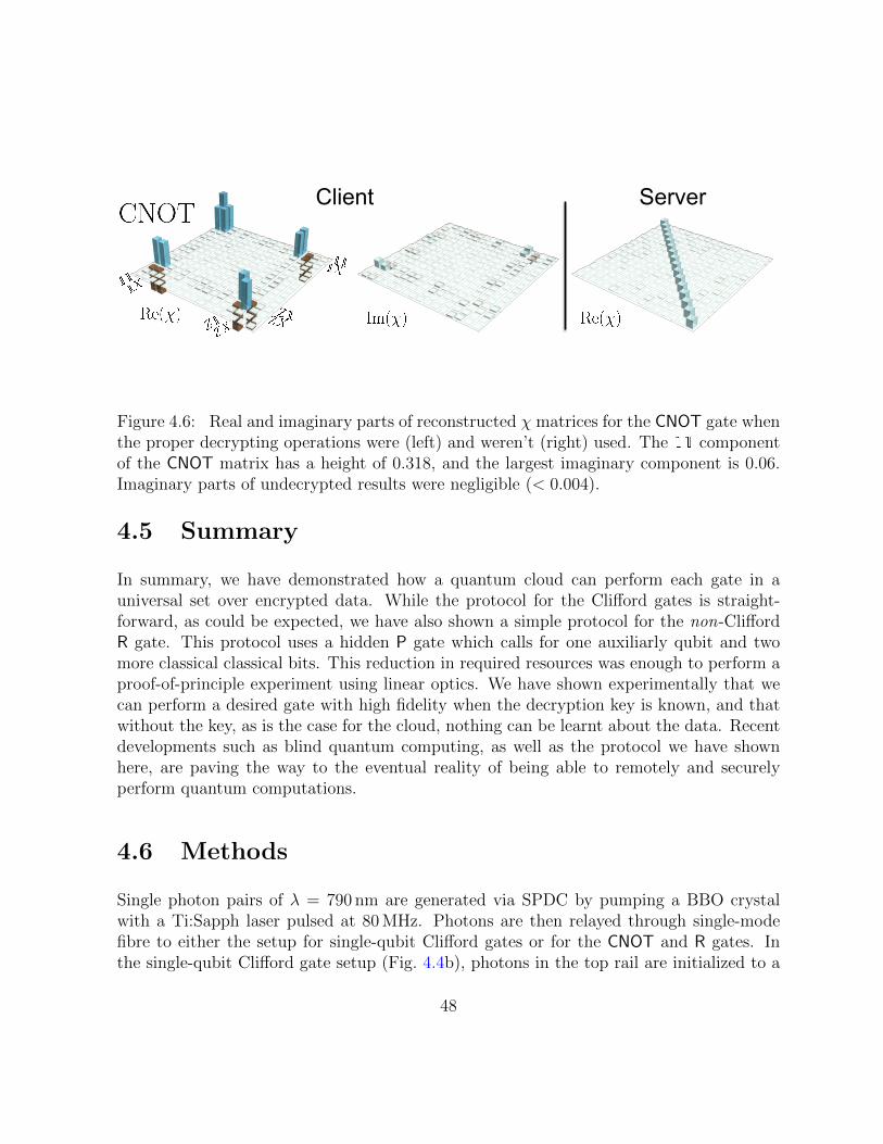
Client Server

Figure 4.6: Real and imaginary parts of reconstructed χ matrices for the CNOT gate whenthe proper decrypting operations were (left) and weren’t (right) used. The 11 componentof the CNOT matrix has a height of 0.318, and the largest imaginary component is 0.06.Imaginary parts of undecrypted results were negligible (< 0.004).

4.5 Summary

In summary, we have demonstrated how a quantum cloud can perform each gate in auniversal set over encrypted data. While the protocol for the Clifford gates is straight-forward, as could be expected, we have also shown a simple protocol for the non-CliffordR gate. This protocol uses a hidden P gate which calls for one auxiliarly qubit and twomore classical classical bits. This reduction in required resources was enough to perform aproof-of-principle experiment using linear optics. We have shown experimentally that wecan perform a desired gate with high fidelity when the decryption key is known, and thatwithout the key, as is the case for the cloud, nothing can be learnt about the data. Recentdevelopments such as blind quantum computing, as well as the protocol we have shownhere, are paving the way to the eventual reality of being able to remotely and securelyperform quantum computations.

4.6 Methods

Single photon pairs of λ = 790 nm are generated via SPDC by pumping a BBO crystalwith a Ti:Sapph laser pulsed at 80 MHz. Photons are then relayed through single-modefibre to either the setup for single-qubit Clifford gates or for the CNOT and R gates. Inthe single-qubit Clifford gate setup (Fig. 4.4b), photons in the top rail are initialized to a

48

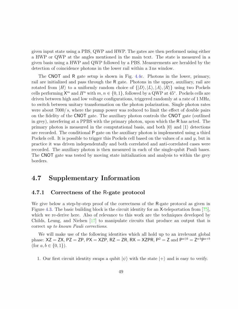
given input state using a PBS, QWP and HWP. The gates are then performed using eithera HWP or QWP at the angles mentioned in the main text. The state is measured in agiven basis using a HWP and QWP followed by a PBS. Measurements are heralded by thedetection of coincidence photons in the lower rail within a 3 ns window.

The CNOT and R gate setup is shown in Fig. 4.4c. Photons in the lower, primary,rail are initialized and pass through the R gate. Photons in the upper, auxiliary, rail arerotated from |H〉 to a uniformly random choice of {|D〉, |L〉, |A〉, |R〉} using two Pockelscells performing Xm and Hn with m,n ∈ {0, 1}, followed by a QWP at 45◦. Pockels cells aredriven between high and low voltage configurations, triggered randomly at a rate of 1 MHz,to switch between unitary transformation on the photon polarization. Single photon rateswere about 7000/ s, where the pump power was reduced to limit the effect of double pairson the fidelity of the CNOT gate. The auxiliary photon controls the CNOT gate (outlinedin grey), interfering at a PPBS with the primary photon, upon which the R has acted. Theprimary photon is measured in the computational basis, and both |0〉 and |1〉 detectionsare recorded. The conditional P gate on the auxiliary photon is implemented using a thirdPockels cell. It is possible to trigger this Pockels cell based on the values of a and y, but inpractice it was driven independentally and both correlated and anti-correlated cases wererecorded. The auxiliary photon is then measured in each of the single-qubit Pauli bases.The CNOT gate was tested by moving state initialization and analysis to within the greyborders.

4.7 Supplementary Information

4.7.1 Correctness of the R-gate protocol

We give below a step-by-step proof of the correctness of the R-gate protocol as given inFigure 4.3. The basic building block is the circuit identity for an X-teleportation from [75],which we re-derive here. Also of relevance to this work are the techniques developed byChilds, Leung, and Nielsen [17] to manipulate circuits that produce an output that iscorrect up to known Pauli corrections.

We will make use of the following identities which all hold up to an irrelevant globalphase: XZ = ZX, PZ = ZP, PX = XZP, RZ = ZR, RX = XZPR, P2 = Z and Pa⊕b = Za·bPa+b

(for a, b ∈ {0, 1}).

1. Our first circuit identity swaps a qubit |ψ〉 with the state |+〉 and is easy to verify.

49

|ψ〉 • |+〉

|+〉 • |ψ〉

2. We can measure the top qubit in the above circuit and classically control the outputcorrection. We have thus re-derived the circuit corresponding to the “X-teleportation”of [75].

|ψ〉 c

|+〉 • Xc|ψ〉

3. Next, we re-define the input to be RXaZb|ψ〉, so the output becomes XcRXaZb|ψ〉 =Xa⊕cZa⊕bPaR|ψ〉.

XaZb|ψ〉 R c

|+〉 • Xa⊕cZa⊕bPaR|ψ〉

4. Then add three gates (Py, Zd, Pa⊕y) to the bottom wire (see circuit below). Usingthe fact that the P and Z commute with control, and applying identities given above,we get as output what we expect:

Pa⊕yZdPyXa⊕cZa⊕bPaR|ψ〉 = Za·yPa+yZdPyXa⊕cZa⊕bPaR|ψ〉 (4.3)

= Zd⊕a·y⊕yPaXa⊕cZa⊕bPaR|ψ〉 (4.4)

= Zd⊕a·y⊕yXa⊕cZa(a⊕c)PaZa⊕bPaR|ψ〉 (4.5)

= Xa⊕cZd⊕a·y⊕y⊕a2⊕a·cZbR|ψ〉 (4.6)

= Xa⊕cZa(c⊕y⊕1)⊕b⊕d⊕yR|ψ〉 (4.7)

XaZb|ψ〉 R c

|+〉 Py Zd • Pa⊕y Xa⊕cZa(c⊕y⊕1)⊕b⊕d⊕yR|ψ〉

4.7.2 Security definition and proof

Preliminaries

Quantum registers and channels. A quantum register is a collection of qubits in somefinite dimensional Hilbert space, say X . We denote D(X ) the set of density operators

50

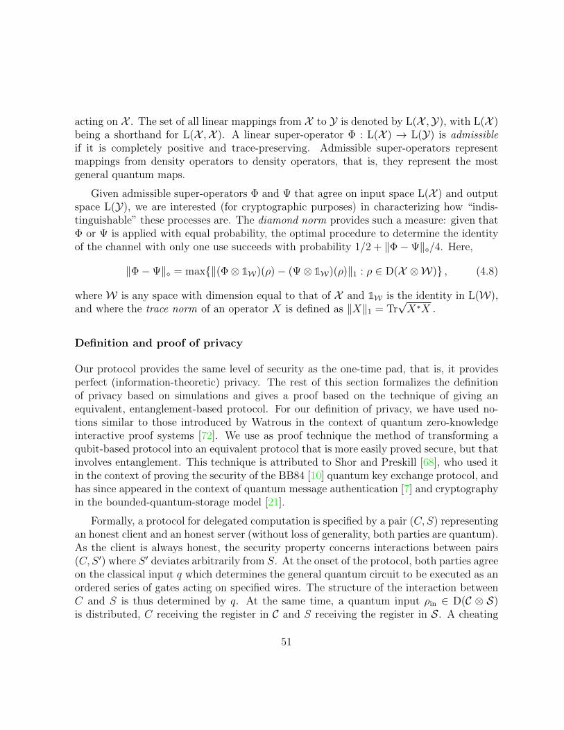
acting on X . The set of all linear mappings from X to Y is denoted by L(X ,Y), with L(X )being a shorthand for L(X ,X ). A linear super-operator Φ : L(X ) → L(Y) is admissibleif it is completely positive and trace-preserving. Admissible super-operators representmappings from density operators to density operators, that is, they represent the mostgeneral quantum maps.

Given admissible super-operators Φ and Ψ that agree on input space L(X ) and outputspace L(Y), we are interested (for cryptographic purposes) in characterizing how “indis-tinguishable” these processes are. The diamond norm provides such a measure: given thatΦ or Ψ is applied with equal probability, the optimal procedure to determine the identityof the channel with only one use succeeds with probability 1/2 + ‖Φ−Ψ‖�/4. Here,

‖Φ−Ψ‖� = max{‖(Φ⊗ 1W)(ρ)− (Ψ⊗ 1W)(ρ)‖1 : ρ ∈ D(X ⊗W)} , (4.8)

where W is any space with dimension equal to that of X and 1W is the identity in L(W),and where the trace norm of an operator X is defined as ‖X‖1 = Tr

√X∗X .

Definition and proof of privacy

Our protocol provides the same level of security as the one-time pad, that is, it providesperfect (information-theoretic) privacy. The rest of this section formalizes the definitionof privacy based on simulations and gives a proof based on the technique of giving anequivalent, entanglement-based protocol. For our definition of privacy, we have used no-tions similar to those introduced by Watrous in the context of quantum zero-knowledgeinteractive proof systems [72]. We use as proof technique the method of transforming aqubit-based protocol into an equivalent protocol that is more easily proved secure, but thatinvolves entanglement. This technique is attributed to Shor and Preskill [68], who used itin the context of proving the security of the BB84 [10] quantum key exchange protocol, andhas since appeared in the context of quantum message authentication [7] and cryptographyin the bounded-quantum-storage model [21].

Formally, a protocol for delegated computation is specified by a pair (C, S) representingan honest client and an honest server (without loss of generality, both parties are quantum).As the client is always honest, the security property concerns interactions between pairs(C, S ′) where S ′ deviates arbitrarily from S. At the onset of the protocol, both parties agreeon the classical input q which determines the general quantum circuit to be executed as anordered series of gates acting on specified wires. The structure of the interaction betweenC and S is thus determined by q. At the same time, a quantum input ρin ∈ D(C ⊗ S)is distributed, C receiving the register in C and S receiving the register in S. A cheating

51

server S ′ is any quantum computational process that interacts with C according to themessage structure determined by q. By allowing S ′ access to the input register S, weexplicitly allow S ′ to share prior entanglement with C’s input; this also models any priorknowledge of S ′ and formalizes the notion that the protocol cannot be used to increaseknowledge.

Let Z denote the output space of S ′ and let Φq : L(S)→ L(Z) be the mapping inducedby the interaction of S ′ with C. Security is defined in terms of the existence of a simulatorSS′ for a given server S ′, which is a general quantum circuit that agrees with S ′ on theinput and output dimensions. Such a simulator does not interact with C, but simplyinduces a mapping Ψq : L(S)→ L(Z) on each input q. Informally, (C, S) is private if thetwo mappings, Φq and Ψq are indistinguishable for every choice of q and every choice of ρin.Allowing for an ε amount of leakage, we formalize this as Definition 1.

Definition 1. A protocol (C, S) for a delegated quantum computation is ε-private if forevery server S ′ there exists a simulator SS′ such that for every classical input q,

‖Φq −Ψq‖� ≤ ε , (4.9)

where Φq is the mapping induced by the interaction of S ′ with the client C on input q andΨq is the mapping induced by SS′ on input q.

Taking ε = 0 gives the strongest possible security against a malicious server: it does notallow for even an ε amount of leakage, and allows the server to deviate arbitrarily (withoutimposing any computational bounds). Theorem 1 states that this is the level of privacyachieved in our protocol.

Our proof technique will construct a sequence of protocols. For clarity, we refer to theprotocol in the main paper as Protocol 1.

Theorem 1. Protocol 1 is an ε-private protocol for delegated quantum computation, withε = 0.

Proof. Fix a value for q. We construct a simulator SS′ by giving instructions how toprepare messages that replace the messages that the client C would send to the server S ′

in the real protocol. Privacy follows since we will show that these transmissions are identicalto those in the real protocol.

A high-level sketch of the proof is that we modify the behaviour of the client in themain protocol (Protocol 1) in a way that the effect of the protocol is unchanged, yet theclient delays introducing her input into the protocol until after her interaction with the

52

server has ended (this makes the simulation almost trivial). In order to do so, we describebelow an entanglement-based protocol (Protocol 2) as well as a delayed-measurementprotocol (Protocol 3).

We first consider Protocol 2, which is an entanglement-based version of Protocol 1.In Protocol 2, we modify how the client prepares her messages, without modifying theserver’s actions or the effect of the protocol. Thus, the preparing and sending of anencrypted quantum register is replaced by an equivalent teleportation-based protocol, asgiven in Figure 4.7. Also, the R-gate protocol is replaced by an equivalent protocol as givenin Figure 4.9. The protocol of Figure 4.9 can be seen to be correct via an intermediateprotocol (Figure 4.8), in which the classical bit x from the client to the server becomesa uniformly random bit; this transformation is possible because in the R-gate protocol,x = a ⊕ y with y a random bit. Then choosing x to be random and y = a ⊕ x givesan equivalent protocol. The final entanglement-based protocol of Figure 4.9 is seen to becorrect via the circuit identity given in Figure 4.10. The remaining protocols for stabilizercircuit elements (Clifford gates, qubit preparation and measurements) are non-interactiveand thus unchanged in Protocol 2.

The main advantage of considering Protocol 2 instead of Protocol 1 is that we candelay all the client’s measurements (in Figures 4.7 and 4.9) until the output register isreturned, without affecting the computation or the server’s view of the protocol (becauseactions on different subsystems commute); call the result Protocol 3. In this delayed-measurement protocol, the messages from the client to the server can be chosen before anyinteraction with the server, and are thus clearly independent of the actions of S ′.

Thus we construct a simulator SS′ that plays the role of the client in Protocol 3, butthat never performs any measurements (thus, access to the actual input is not required).By the argument above, SS′ actually prepares the same transmissions as would C inProtocol 1 interacting with S ′ on any input ρin. It follows that simulating S ′ on thesetransmissions will induce the same mapping as S ′ in the real protocol, and thus ‖Φq −Ψq‖� = 0 .

53

Server XaZb|ψ〉

Client|0〉 H •

|0〉 a

|ψ〉 • H b

Figure 4.7: Protocol to encrypt and send a qubit using teleportation[11]. The circuit inthe dashed box prepares an EPR-pair.

XaZb|ψ〉 R •

Server • •

• Px Xa⊕cZa(c⊕y⊕1)⊕b⊕d⊕yR|ψ〉

Clientx ∈R {0, 1} • • c

|+〉 Py Zd (d ∈R {0, 1}, y = a⊕ x)

Figure 4.8: Intermediate Protocol for an R-gate. Compared to Figure 4.3, the classicalmessage from the client to the server is chosen uniformly at random. This protocol performsthe same computation as the protocol in Figure 4.3.

XaZb|ψ〉 R •

Server • •

• Px Xa⊕cZa(c⊕y⊕1)⊕b⊕d⊕yR|ψ〉

x ∈R {0, 1} • • c

Client |0〉 H • (y = a⊕ x)

|0〉 Py H d

Figure 4.9: Entanglement-based protocol for an R-gate. This protocol performs the samecomputation as the protocols in Figures 4.3 and 4.8. The circuit in the dashed box preparesan EPR-pair.

54

|0〉 H • ZdPy|+〉

|0〉 Py H d

Figure 4.10: Circuit identity: entanglement-based circuit that prepares a qubit ZdPy|+〉 foruniformly random bits y and d (here, y is chosen uniformly at random, and d is determinedby the measurement). The circuit in the dashed box prepares an EPR-pair.

55

Chapter 5

Conclusion

In this thesis we have covered a broad spectrum of quantum information processing withlinear optics. In Chapter 3, we demonstrated an optimal realization of a single-dampingchannel. This channel could add a controllable amount and type of decoherence to a qubit.We characterized the channel using a novel ancilla-assisted quantum process tomography,where we took into account the imperfection of the two-qubit resource state.

A natural next step is to implement a recently developed error correction code for thedetected jump channel [31], which is the amplitude damping channel where the decay ismarked by the detection of a photon. The error correction protocol calls for the use of aCNOT gate, which was also implemented in this thesis. Realizing this correction schemewill require constructing and characterizing a second amplitude damping channel to runin parallel with the current one.

In Chapter 4 we showed the implementation of a protocol for performing quantumcomputations on encrypted data. We showed that for each quantum gate in a universalset that if data is encrypted and decrypted properly the proper action of the gate isobserved, and with high fidelity. On the other hand, if the proper decryption is not known,as is the case for an eavesdropper, the gate becomes a completely depolarizing channel,mapping every state to the maximally-mixed state. A next step in this work might includeperforming some simple algorithms, such as a two-qubit Grover search, over encrypteddata.

56

APPENDICES

57

Appendix A

Configuring Pockels cells

The Pockels cells used in the experiment in Chapter 4 were purchased from Bergmann Mess-geraete Entwicklung KG (BME). They drive a rubidium titanyl phosphate, RbTiOPO4

(RTP), with voltage oscillating between high (set to given the desired amount of retar-dance, polarization rotation). We drove the Pockels cells between ±Vλ/4, using splitterboxes electronics designed by Thomas Jennewein and programmed by Zhizhong Yan. Thisdifferent from previous experiments which operated the cells between 0 and Vλ/2.

The basic protocol for aligning and configuring a Pockels cell follows these steps.

1. Aligning the isogyre (Fig. A.1). An isogyre is an image which results from send-ing polarized and somewhat dispersed light through a birefringent material (Pockelscell) and placing a crossed polarizer on the other end. Light propagating along thematerial’s optic axis will not change polarization and will be absorbed by the sec-ond polarizer, leaving a dark line in the resulting image, showing where the axis is.Ideally, the isogyre image is a cross, but some alignment is required to observe this.Here we performed many iterations of:

(a) Using 2 of the 4 tilting degrees of freedom in the Pockels cell to back reflect thecrystal.

(b) Using the other 2 degrees of freedom to centre the isogyre crossing on the ob-served image (Note that until properly aligned, the dark bands may not forma cross, but rather look like an avoided crossing. But just keep repeating thesteps and it will all be fine.)

2. Use single photons in a setup like that of Fig. A.2a.

58

screen

PC PBS PBS

isogyre

Figure A.1: Polarized light is dispersed through some cloudy screen (a sticky note wasused) and propagated through the birefringent Pockels cell. Placing a crossed polarizerafterwards allows for the observation of the isogyre, an image which when properly alignedlooks like a cross.

3. Send in each of two orthogonal input states (eg. |H〉 and |V 〉), and looking atcoincidence counts, vary driving voltage while measuring the state you expect outputfrom the Pockels cell when the voltage is high (eg., for a Hadamard 〈D| and |A〉).Choose the voltage that gives the best contrast between the two measurement bases.

4. Same as step 3, but vary the angle δ, changing the HWPs and QWP, to find the bestcontrast again.

5. Same as steps 3 and 4, but now vary the delay of the signal into the Pockels cell.The idea here is that when the Pockels changes from low to high voltage states, thereis some “ringing”, meaning the voltage is not instantly constant at the desired Vλ/4,and so changes the desired rotation. (Note that for the experiment in Chapter 4, wedid not have to perform this step).

6. Iterate step 3-5 until the the contrast is reasonably high (∼ 100 : 1 should be easyto attain. With changing the delay ∼ 1000 : 1 is possible).

The tables below show an example of data taken when configuring the second Pockelscell (performing 1/H). First, we set all the waveplates such that δ = 0. We send in |H〉and |V 〉 and scan over the voltage while measuring coincidence counts over 5 seconds inboth 〈A| and 〈D|, to find the best contrast.

59

PC  

QWP PBS

Analyzer

PC OFF PC Low PC High

a

b c d

HWP

Initalize state

Figure A.2: (a) A simple setup to configure the Pockels cell. Photons are initialized as |H〉from the PBS. The Pockels cell is sandwiched by HWPs, and a QWP. Finally, a polarizationanalyzer and photon detection. Coincidence counts with another photon detection shouldbe used. (b)–(d) show the action of the HWP-PC-QWP-HWP setup when the Pockels cellis OFF, at low voltage, and at high voltage, respectively. For this example, the desiredoperation of the setup is to perform the identity when the PC is at low voltage, and anX rotation at high voltage. Recall from the discussion in Chapter 2 that this requires theHWPs to be at δ◦, and the QWP at (45 + δ)◦ (since the PC crystal is aligned at (45 + δ)◦

where |δ| � 1 ).

60

|H〉 |V 〉V (dial) 〈A| 〈D| 〈A| 〈D|

1.5 156 3437 3382 611.6 113 3371 3255 591.7 96 3482 3248 561.8 69 3335 3135 611.9 56 3402 3153 842.0 40 3338 3101 852.1 52 3334 3071 1172.2 45 3323 3118 1922.3 64 3325 3009 217

The best contrast for |H〉 is ∼ 83 : 1 at V = 2.0. For |V 〉 it is ∼ 58 : 1 at V = 1.7.We then set the voltage to V = 1.85, in between the two optima. Next, with the voltageset, we vary the angle discrepancy δ, changing the angle of each waveplate. We measurecoincidence counts over 5 seconds for both 〈A| and |D〉. Sending in |H〉 and |V 〉 we get:

|H〉 |V 〉δ(◦) 〈A| 〈D| 〈A| 〈D|-3 72 3487 3374 40-2 55 3471 3441 20-1 47 3568 3391 270 61 3547 3387 521 112 3341 3432 138

The best constrast for |H〉 is ∼ 76 : 1 at δ = −1◦, and for |V 〉 is ∼ 172 : 1 at δ = −2◦.The next step would be to scan over the delay time of the input signal to the Pockels cell.However, because of the nature of the experiment in Chapter 4, the time intervals for PCswitching where long in comparison to other experiments, and so fine tuning of the delaywas not necessary. Taking δ = −1.5◦, we again scan over the voltage:

61

|H〉 |V 〉V (dial) 〈A| 〈D| 〈A| 〈D|

1.6 94 2982 2798 141.65 65 2874 2833 171.7 66 2984 2845 131.75 59 3072 2757 251.8 57 3047 2674 151.85 30 2901 2706 271.9 35 2993 2656 361.95 34 3114 2671 332.0 19 3113 2826 512.05 36 2962 2758 572.1 14 2931 2830 672.15 18 2972 2817 762.2 25 2955 2684 102

The best contrasts are again at V = 2.1 for |H〉 and V = 1.7 for |V 〉, are greatlyimproved (∼ 209 : 1 and ∼ 218 : 1). Taking the voltage to be in between, V = 1.85 we getcontrasts ∼ 100 : 1 for both inputs.

Figure A.3 shows the splitter box and electronics setup for Pockels cells in Chapter 4.

62

Electronics setup

Splitter Boxes

To PC 1 To PC 2 To PC 3

AND

DAQ (1 MHz)

Photon  Detector  

Coinc. Logic

Func. Gen. (6 MHz)

phot. 2 phot. 1

Figure A.3: Detected photons cause a TTL pulse to be generated from the single-photoncounting modules. TTL pulses are passed through an array of AND logic with the square-wave pulses which drove the Pockels cell, originally produced from the DAQ. This resultsin TTL pulses sorted into times when the Pockels cell were acting as the identity, or as theassigned unitary.

63

Appendix B

Imperfection in the CNOT gate

B.1 Imperfect interference

The operation of the optical CNOT entirely depends on the quality of the two-photoninterference at the initial partially-polarizing beamsplitter (PPBS). We used a motorizedstage to adjust path delays, ensuring that we were operating the gate in the bottom of theHOM dip, which had the desired visibility. Nonetheless, we can see the effects of imperfectinterference on the measured output state. This could be due to path lengths driftingover the course of the experiment. As can be seen in Fig. B.1, we have non-negligiblecontributions to the density matrix from what looks like a mixture of |DH〉〈DH| and|V A〉〈V A|.

This can explained by considering the state |DaHb〉 in input modes a and b. Sincethey don’t interfere at the PPBS we can consider their propagations through the setupseparately. Recall from CNOT setup outlined in Chapter 2, that we begin with a Hadamardgate in path b before a and b modes interfere at a PPBS. Half-wave plates (HWP) at 45◦ arenext, followed by another PPBS in each mode, now called c and d. Batears then performan X operation on each mode, and finally another Hadamard acts on mode d. The |Da〉state then propagates as follows:

64

Figure B.1: The real (a) and imaginary (b) parts of an output density matrix from theCNOT. The input state was |DH〉.

|Da〉 =1√2

(a†H + a†V

)|0〉

PPBS−−−→ 1√2

(c†H +

1√3c†V +

√2

3d†V

)|0〉

HWPs−−−→ 1√2

(c†V +

1√3c†H +

√2

3d†H

)|0〉

PPBS−−−→ 1√2

(1√3c†V +

1√3c†H +

√2

3d†H

)|0〉

batears−−−−→ 1√3

(c†D + d†V

)|0〉

1⊗H−−−→ 1√3

(c†D + d†A

)|0〉

=1√3

(|Dc〉+ |Ad〉) (B.1)

The input state |Hb〉 propagates as:

65

|Hb〉 = b†H |0〉1⊗H−−−→ 1√

2

(b†H + b†V

)|0〉

PPBS−−−→ 1√2

(d†H +

1√3d†V −

√2

3c†V

)|0〉

HWPs−−−→ 1√2

(d†V +

1√3d†H −

√2

3c†H

)|0〉

PPBS−−−→ 1√2

(1√3d†V +

1√3d†H −

√2

3c†H

)|0〉

batears−−−−→ 1√3

(d†D − c

†V

)|0〉

1⊗H−−−→ 1√3

(−c†V + d†D

)|0〉

=1√3

(−|Vc〉+ |Dd〉) (B.2)

Since we measure coincidence photons between c and d modes, we would measure amixture of |DcAd〉 and |VcAd〉. Moving the motor stage to completely outside of the HOMdip, this is precisely what we observe, see Fig. B.2. Refer back to Fig.B.1 and notice thatthesis components are clearly visible in the density matrix, and diminish the state fidelitywith the ideal Bell state.

66

Figure B.2: Theoretical (a) and measured (b) density matrices for propagating |DH〉through the CNOT setup when operating outside of the HOM dip. These components arestill clearly visible when trying to operate the CNOT with the HOM dip.

67

References

[1] D. Aharonov, M. Ben-Or, and E. Eban. Interactive proofs for quantum computations.In Proceeding of Innovations in Computer Science 2010 (ICS 2010), pages 453–469,2010.

[2] M. P. Almeida, F. de Melo, M. Hor-Meyll, A. Salles, S. P. Walborn, P. H. SoutoRibeiro, and L. Davidovich. Environment-induced sudden death of entanglement.Science, 316(5824):579–582, 2007.

[3] J. B. Altepeter, D. Branning, E. Jeffrey, T. C. Wei, P. G. Kwiat, R. T. Thew, J. L.O’Brien, M. A. Nielsen, and A. G. White. Ancilla-assisted quantum process tomog-raphy. Phys. Rev. Lett., 90:193601, May 2003.

[4] A. Ambainis, M. Mosca, A. Tapp, and R. De Wolf. Private quantum channels. InProceedings of the 41st Annual IEEE Symposium on Foundations of Computer Science(FOCS 2000), pages 547–553, 2000.

[5] P. Arrighi and L. Salvail. Blind quantum computation. Int. J. Quantum Inf., 4:883898,2006.

[6] K. Banaszek, G. M. D’Ariano, M. G. A. Paris, and M. F. Sacchi. Maximum-likelihoodestimation of the density matrix. Phys. Rev. A, 61:010304, Dec 1999.

[7] H. Barnum, C. Crepeau, D. Gottesman, A. Smith, and A. Tapp. Authenticationof quantum messages. In Proceedings of the 43rd Annual IEEE Symposium on theFoundations of Computer Science (FOCS ’02), pages 449–458, 2002.

[8] S. Barz, E. Kashefi, A. Broadbent, J. F. Fitzsimons, A. Zeilinger, and P. Walther.Demonstration of blind quantum computing. Science, 20:303–308, 2012.

[9] J.S. Bell. On the Einstein-Podolsky-Rosen paradox. Physics, 1:195, 1964.

68

[10] C. H. Bennett and G. Brassard. Quantum cryptography: Public key distribution andcoin tossing. In Proceedings of the IEEE International Conference on Computers,Systems, and Signal Processing, pages 175–179, 1984.

[11] C .H. Bennett, G. Brassard, C. Crepeau, R. Jozsa, A. Peres, and W. Wootters. Tele-porting an unknown quantum state via dual classical and Einstein-Podolsky-Rosenchannels. Physical Review Letters, pages 1895–1899, 1993.

[12] R.W. Boyd. Nonlinear Optics. Academic Press. Academic Press, 2008.

[13] S. Bravyi and A. Kitaev. Universal quantum computation with ideal Clifford gatesand noisy ancillas. Physical Review A, 71:022316, 2005.

[14] H.J. Briegel, D.E. Browne, W. Dur, R. Raussendorf, and M. Van den Nest.Measurement-based quantum computation. Nature Physics, 5(1):19–26, 2009.

[15] A. Broadbent, J. Fitzsimons, and E. Kashefi. Universal blind quantum computation.In Proceedings of the 50th Annual IEEE Symposium on Foundations of ComputerScience (FOCS 2009), pages 517–526, 2009.

[16] A. Childs. Secure assisted quantum computation. Quantum Information and Com-putation, 5:456–466, 2005.

[17] A. M. Childs, D. W. Leung, and M. A. Nielsen. Unified derivations of measurement-based schemes for quantum computation. Physical Review A, 71:032318, 2005.

[18] M.-D. Choi. Completely positive linear maps on complex matrices. Linear Algebraand its Applications, 10(3):285 – 290, 1975.

[19] J. M. Chow, J. M. Gambetta, L. Tornberg, Jens Koch, Lev S. Bishop, A. A. Houck,B. R. Johnson, L. Frunzio, S. M. Girvin, and R. J. Schoelkopf. Randomized bench-marking and process tomography for gate errors in a solid-state qubit. Phys. Rev.Lett., 102:090502, Mar 2009.

[20] M. Christandl and S. Wehner. Quantum anonymous transmissions. In Bimal Roy,editor, Advances in Cryptology - ASIACRYPT 2005, volume 3788 of Lecture Notes inComputer Science, pages 217–235. Springer Berlin / Heidelberg, 2005.

[21] I. B. Damgard, S. Fehr, L. Salvail, and C. Schaffner. Cryptography in the bounded-quantum-storage model. In Proceedings of the 46th IEEE Symposium on Foundationsof Computer Science (FOCS 2005), 2005. Full version in SIAM Journal on Comput-ing 37:1865-1890, 2008.

69

[22] D. Deutsch and R. Jozsa. Rapid Solution of Problems by Quantum Computation.Proceedings of the Royal Society A: Mathematical, Physical and Engineering Sciences,439(1907):553–558, December 1992.

[23] I. Devetak and P. W. Shor. The capacity of a quantum channel for simultaneoustransmission of classical and quantum information. Communications in MathematicalPhysics, 256:287–303, 2005. 10.1007/s00220-005-1317-6.

[24] A. Fedrizzi, T. Herbst, A. Poppe, T. Jennewein, and A. Zeilinger. A wavelength-tunable fiber-coupled source of narrowband entangled photons. Opt. Express,15(23):15377–15386, Nov 2007.

[25] S. Fehr and C. Schaffner. Composing quantum protocols in a classical environment.In Proceedings of the Theory of Cryptography Conference (TCC ’09), pages 350–367,2009.

[26] R. P. Feynman. Simulating physics with computers. International Journal of Theo-retical Physics, 21(6-7):467–488, June 1982.

[27] J. Fiurasek and Z. Hradil. Maximum-likelihood estimation of quantum processes.Phys. Rev. A, 63:020101, Jan 2001.

[28] C. Gentry. Fully homomorphic encryption using ideal lattices. In Proceedings of the41st annual ACM symposium on Theory of Computing (STOC ’09), pages 169–178,2009.

[29] A. Gilchrist, N. K. Langford, and M. A. Nielsen. Distance measures to compare realand ideal quantum processes. Phys. Rev. A, 71:062310, Jun 2005.

[30] D. Gottesman. The Heisenberg representation of quantum computers. In Group 22:Proceedings of the XXII International Colloquium on Group Theoretical Methods inPhysics, pages 32–43, 1998.

[31] Markus Grassl, Zhengfeng Ji, Zhaohui Wei, and Bei Zeng. Quantum-capacity-approaching codes for the detected-jump channel. Phys. Rev. A, 82:062324, Dec 2010.

[32] L. K. Grover. A fast quantum mechanical algorithm for database search. In ANNUALACM SYMPOSIUM ON THEORY OF COMPUTING, pages 212–219. ACM, 1996.

[33] M. B. Hastings. Superadditivity of communication capacity using entangled inputs.Nature Physics, 5:255–257, April 2009.

70

[34] B. Hayes. Cloud computing. Commun. ACM, 51(7):9–11, July 2008.

[35] C. W. Helstrom. Detection theory and quantum mechanics. Information and Control,10(3):254–291, 1967.

[36] M. Hillery and L. D. Mlodinow. Quantization of electrodynamics in nonlinear dielectricmedia. Phys. Rev. A, 30:1860–1865, Oct 1984.

[37] C. K. Hong, Z. Y. Ou, and L. Mandel. Measurement of subpicosecond time intervalsbetween two photons by interference. Phys. Rev. Lett., 59:2044–2046, Nov 1987.

[38] M. Horodecki, P. Horodecki, and R. Horodecki. Mixed-state entanglement and distil-lation: Is there a “bound” entanglement in nature? Phys. Rev. Lett., 80:5239–5242,Jun 1998.

[39] Z. Hradil and Rehacek J. Quantum measurement and information. Fortschritte derPhysik, 51(2-3):150–156, 2003.

[40] D. F. V. James, P. G. Kwiat, W. J. Munro, and A. G. White. Measurement of qubits.Phys. Rev. A, 64:052312, Oct 2001.

[41] R. Jozsa. Fidelity for mixed quantum states. Journal of Modern Optics, 41(12):2315–2323, 1994.

[42] N. Kiesel, C. Schmid, U. Weber, R. Ursin, and H. Weinfurter. Linear optics controlled-phase gate made simple. Phys. Rev. Lett., 95:210505, Nov 2005.

[43] A. Yu. Kitaev. Quantum computations: algorithms and error correction. RussianMathematical Surveys, 52(6):11911249, 1997.

[44] E. Knill, R. Laflamme, and G. J. Milburn. A scheme for efficient quantum computationwith linear optics. Nature, 409(6816):46–52, January 2001.

[45] A. Jamio lkowski. Linear transformations which preserve trace and positive semidefi-niteness of operators. Reports on Mathematical Physics, 3(4):275 – 278, 1972.

[46] N. K. Langford, T. J. Weinhold, R. Prevedel, K. J. Resch, A. Gilchrist, J. L. O’Brien,G. J. Pryde, and A. G. White. Demonstration of a simple entangling optical gate andits use in bell-state analysis. Phys. Rev. Lett., 95:210504, Nov 2005.

[47] J.-C. Lee, Y.-C. Jeong, Y.-S. Kim, and Y.-H. Kim. Experimental demonstra-tion of decoherence suppression via quantum measurement reversal. Opt. Express,19(17):16309–16316, Aug 2011.

71

[48] N. Lutkenhaus, J. Calsamiglia, and K.-A. Suominen. Bell measurements for telepor-tation. Phys. Rev. A, 59:3295–3300, May 1999.

[49] A I Lvovsky. Iterative maximum-likelihood reconstruction in quantum homodynetomography. Journal of Optics B: Quantum and Semiclassical Optics, 6(6):S556,2004.

[50] G. J. Milburn. Quantum optical fredkin gate. Phys. Rev. Lett., 62:2124–2127, May1989.

[51] P.W. Milonni and J.H. Eberly. Laser Physics. John Wiley & Sons, 2010.

[52] M.A. Nielsen and I.L. Chuang. Quantum Computation and Quantum Information:10th Anniversary Edition. Cambridge University Press, 2010.

[53] J. L. O’Brien, G. J. Pryde, A. Gilchrist, D. F. V. James, N. K. Langford, T. C. Ralph,and A. G. White. Quantum process tomography of a controlled-not gate. Phys. Rev.Lett., 93:080502, Aug 2004.

[54] J. L. O’Brien, G. J. Pryde, A. G. White, T. C. Ralph, and D. Branning. Demonstrationof an all-optical quantum controlled-NOT gate. Nature, 426(6964):264–7, November2003.

[55] D. W. Leung P. H. Hayden and D. Mayers. The universal composable security ofquantum message authentication with key recycling. Unpublished manuscript, 20xx.

[56] Marco Piani, David Pitkanen, Rainer Kaltenbaek, and Norbert Lutkenhaus. Linear-optics realization of channels for single-photon multimode qudits. Phys. Rev. A,84:032304, Sep 2011.

[57] R. Prevedel, D. R. Hamel, R. Colbeck, K. Fisher, and K. J. Resch. Experimentalinvestigation of the uncertainty principle in the presence of quantum memory and itsapplication to witnessing entanglement. Nature Physics, 7(10):757–761, July 2011.

[58] L. Qing, L. Jian, and G. Guang-Can. Linear optical realization of qubit purificationwith quantum amplitude damping channel. Chinese Physics Letters, 24(7):1809, 2007.

[59] T. C. Ralph, N. K. Langford, T. B. Bell, and A. G. White. Linear optical controlled-not gate in the coincidence basis. Phys. Rev. A, 65:062324, Jun 2002.

[60] R. Raussendorf and H. J. Briegel. A one-way quantum computer. Phys. Rev. Lett.,86:5188–5191, 2001.

72

[61] R. Raussendorf, D. E. Browne, and H. J. Briegel. Measurement-based quantum com-putation with cluster states. Physical Review A, 68:022312 [32 pages], 2003.

[62] K. J. Resch, P. Walther, and A. Zeilinger. Full characterization of a three-photongreenberger-horne-zeilinger state using quantum state tomography. Phys. Rev. Lett.,94:070402, Feb 2005.

[63] R. Rivest, L. Adleman, and M. Dertouzos. On data banks and privacy homomor-phisms. In Foundations of Secure Computation, pages 169–177, 1978.

[64] R. Rivest, A. Shamir, and L. Adleman. A method for obtaining digital signatures andpublic-key cryptosystems. Communications of the ACM, 21:120–126, 1978.

[65] B. Rosgen and J. Watrous. On the hardness of distinguishing mixed-state quantumcomputations. In Proceedings of the 20th Conference on Computational Complexity,pages 344–354, 2005.

[66] C. Shannon. Communication theory of secrecy systems. Bell System Technical Jour-nal, 28(4):656–715, 1949.

[67] P. W. Shor. Polynomial-Time Algorithms for Prime Factorization and Discrete Log-arithms on a Quantum Computer. SIAM J. Comput., 26(5):1484–1509, 1997.

[68] P. W. Shor and J. Preskill. Simple proof of security of the BB84 quantum key distri-bution protocol. Physical Review Letters, 85:441–444, 2000.

[69] G. Smith and J. Yard. Quantum communication with zero-capacity channels. Science(New York, N.Y.), 321(5897):1812–5, September 2008.

[70] R. R. Smith. Completely bounded maps between C∗-algebras. Journal of the LondonMathematical Society, s2-27(1):157, 1983.

[71] J. Rehacek, D. Mogilevtsev, and Z. Hradil. Tomography for quantum diagnostics.New Journal of Physics, 10(4):043022, 2008.

[72] J. Watrous. Zero-knowledge against quantum attacks. SIAM Journal on Computing,39:25–58, 2009. Preliminary version in Proceedings of the 38th ACM Symposium onTheory of Computing (STOC ’06), pages 296–305, 2006.

[73] M. M. Wolf and D. Perez-Garcia. Quantum capacities of channels with small envi-ronment. Phys. Rev. A, 75:012303, Jan 2007.

73

[74] W. K. Wootters. Entanglement of formation of an arbitrary state of two qubits. Phys.Rev. Lett., 80:2245–2248, Mar 1998.

[75] X. Zhou, D. Leung, and I. L. Chuang. Methodology for quantum logic gate construc-tion. Physical Review A, 62:052316, 2000.

74