Implementing a Dual Income Tax in Germany: Effects on Investment and Welfare

Doina Maria Radulescu Michael Stimmelmayr

Ifo Working Paper No. 20

November 2005

An electronic version of the paper may be downloaded from the Ifo website: www.ifo.de

brought to you by COREView metadata, citation and similar papers at core.ac.uk

provided by Research Papers in Economics

Ifo Working Paper No. 20

Implementing a Dual Income Tax in Germany: Effects on Investment and Welfare

Abstract This paper investigates the effects of implementing a dual income tax (DIT) in Ger-many. We follow the reform proposal of the German Council of Economic Advisors (2003) and analyze its implications on capital formation, investment and welfare using a dynamic computable general equilibrium model. The main features of the model are an intertemporal investment model and the traditional Ramsey model on the household side. Our findings suggest that the introduction of a DIT with a proportional capital in-come tax rate of 30% and progressive labour income tax rates up to 35% leads to higher investments, an increased capital accumulation up to 5.8% and welfare gains of about 1% of GDP. JEL Code: C68, D58, D92, E62, H25. Keywords: Capital income taxation, computable general equilibrium modelling, welfare analysis.

Doina Maria Radulescu Ifo Institute for Economic Research

at the University of Munich Poschingerstr. 5

81679 Munich, Germany Phone: +49(0)89/9224-1336

radulescu@ifo.de

Michael Stimmelmayr Center for Economic Studies

University of Munich Schackstr. 4

80539 Munich, Germany Phone: +49(0)89/2180-2087

stimmelmayr@ces.vwl.uni-muenchen.de

1 Introduction

A redesign of the German tax system is imperatively required since the present tax law

is complicated, non-transparent and a major obstacle for the country to survive in the

international tax competition. Double taxation and legal tax loopholes create severe

distortions concerning the investment and financial decisions of firms resulting in major

welfare losses. In the light of recent discussions, especially brought about by the report

of the German Council of Economic Advisors (GCEA,2003), a dual income tax

(DIT) has become increasingly popular as an option for reforming the German tax system.

A DIT, which has been applied in several Nordic countries and practiced in Austria and

Belgium in some rudimentary form, would not only reduce these distortions but also

create substantial efficiency gains.

We use a computable general equilibrium growth model calibrated to the German

economy and consisting of four blocks. Optimal investment behavior is derived from

a neoclassical, intertemporal investment model with convex adjustment costs. Since we

mainly focus on the efficiency effects of the tax reform on welfare, we model the household

sector using the traditional Ramsey model of an infinitely lived household. The public

sector introduces various distortions on agents’ behavior through taxation. The model’s

fourth building block is the Rest of the World (RoW), which closes the model. While the

home economy is considered in detail, the foreign economy is only roughly modelled.

Following the proposal made by the GCEA (2003), we measure the economic effects

such a reform would have. Our findings suggest that the introduction of the proposed

dual income tax with a proportional capital income tax rate of 30 per cent and progressive

1

labour income tax rates up to 35 per cent leads to higher investments and an increased

capital accumulation. The calculated 5.8 per cent increase in the capital stock is mainly

driven by a nine per cent reduction in the cost of capital as a result of the major reduction

in statutory tax rates on the corporate and household level. Moreover, GDP and welfare

in terms of life-time income also rise by 3.3 and 1.6 per cent respectively.

The next section of the paper describes the experiences of Nordic countries with the

dual income tax and presents the advantages and shortcomings of such a tax. Section

three introduces the baseline model and derives several important behavioral responses as

well as comparative static results. Section four discusses the simulation results, which are

checked with regard to their robustness by a sensitivity analysis. Finally, the conclusion

highlights the most important findings.

2 The DIT - An Option for Germany

Germany, the country of the ‘Wirtschaftswunder’ and once the leader of European growth

statistics, has now fallen behind most other European countries in terms of growth. Ger-

many faces persistent structural problems and a weak economic climate which is among

other factors also the result of the increased tax competition. Moreover, according to

the GCEA (2003), the tangled mass of partly proposed, partly enforced tax reliefs and

modifications in the tax system have not led to much improvement but induced a cred-

ibility loss, resulting in decreasing investments. Furthermore, the partial alteration of

the tax system, has undermined the principles underlying the comprehensive income tax

system and led to many distortions concerning investment behavior, financial decisions

2

or the organizational choice of a firm. While the German income tax system is still per-

ceived to be a comprehensive one, it systematically deviates from this principle in reality;

e.g. distributed profits are taxed differently than earnings stemming from other sources

according to the half-income principle of dividend taxation. Additional anomalies arise

due to the multitude of tax exemptions, including for instance returns from institutional

savings or capital gains. Another incompatibility consists in the methodical difference of

determining the respective tax base of labor and capital income.1

2.1 Reasons for a Schedular Tax System

There are several reasons for applying different tax rates for labour and capital. Thus,

a lower capital income tax rate as given by the DIT could substantially reduce the in-

tertemporal distortions related to the saving-consumption decision. These distortions are

the result of a double taxation phenomenon: Savings stem from after tax earned income

and returns from saving are taxed once again when they occur. To avoid this additional

burden on future consumption, no capital income tax should exist. However, this is not

always feasible and thus a lower capital income tax rate compared to the labour income

tax rate is desirable (Boadway, 2004).

Moreover, the present tax competition presents an additional argument for taxing

the internationally mobile factor capital at a lower rate. Despite the recent tax reliefs,

1While the capital income tax base is determined on the accrual basis (difference in wealthbetween the beginning and end of each tax period), the labor tax base is calculated on a cashbasis (difference between revenue arising from labour supply and the expenses needed to achievethis revenue). Thus, income stemming from labour enjoys tax privileges, since expenses linkedto human capital investments are immediately deductible, while those required for capital in-vestments can only be deducted later on via depreciation (Wagner, 2000).

3

Germany’s effective tax rates are still among the highest within Europe (European

Commission 2001). Albeit the statutory corporate tax rate amounts to only 25 per cent,

adding the local trade tax and the solidarity surcharge the effective tax rate on profits

adds up to 38.7 per cent, while the EU 15 average is 29.4 per cent, the OECD average

is just 29 per cent and the average among the ten new EU members only 16.p per cent.

Therefore, Germany will have to lower its capital income tax rates further to prevent

capital from fleeing to low tax countries.

Last but not least, the production efficiency theorem2 states that a wage tax solely

distorts the consumption decision, while a source tax on capital also distorts the interna-

tional capital allocation resulting in a deadweight loss.

Therefore, these arguments favour levying a lower tax rate on capital vis-a-vis labour.

The empirical findings of instance by Mendoza et al. (1994), Devereux et al.

(2002) or Sørensen (2000) also suggest a shift of the tax burden towards labour in-

come.3 Thus, both, theory and empirical evidence provide multiple arguments in favour

of introducing a DIT.

2See Diamond and Mirrlees (1971).3Mendoza et al. construct time series of tax rates for seven OECD countries from 1965-

1988 using national accounts and revenue statistics. Their findings suggest inter alia that there isa moderate shift of the tax burden towards labour. Devereux et al. (2002) provide evidencefor the international trend towards lower tax rates on capital. Similar conclusions are derived bySørensen (2000) who computes average effective tax rates on labour and capital respectivelyfor 12 countries for the periods 1981-1985 and 1991-1995. His results show that while the taxburden on labour increased, the burden on capital declined or remained constant.

4

2.2 The Experience of Nordic Countries

Looking for an adequate option for reforming the German tax system one may notice that

similar problems were solved in the Nordic Countries by introducing a DIT a decade ago.

Several papers like Sørensen (2001), Cnossen (2000), and Sørensen/Nielsen (1997)

discuss the experiences these countries had with such a tax system. Starting with Denmark

in 1987, followed by Sweden in 1991, and Norway and Finland in the subsequent years, all

four countries changed their tax system from a comprehensive income tax to a schedular

one. The modifications included a reduction in statutory capital income tax rates to 28

per cent in Norway (IBFD 2004) and Finland and 30 per cent in Denmark (European

Tax Handbook 2004). Simultaneously, the existing tax base was broadened such that

major losses in aggregate tax revenue were prevented. Additionally, a progressive tax

schedule, ranging between 28 to 41.5 per cent in Norway, or 39.7 to 59 per cent in Denmark

was levied on labour income (Mennel/Förster 2003). Regarding the double taxation

of distributed profits, Norway and Finland avoided this by applying full imputation.

The double taxation of retained profits was abolished only in Norway. Furthermore,

withholding or source taxes were installed at the company level or at the level of interest,

royalty or other types of capital income paying entities, to guarantee the single taxation

of capital income.

2.3 The Concept of a Dual Income Tax

The dual income tax can be ascribed to the theoretical model of the Johansson-Samuelson

tax, which taxes only the true economic profit. Such a tax is levied uniformly on all types

5

of income that have been determined in an identical way in the country of residence. Since

income cannot always be computed in the same way, different tax rates may be necessary

to adjust the differences in the computation of the tax base. Accordingly, a pure DIT

distinguishes between capital and labour income. Capital income — including business

profits, dividends, capital gains, interest and rental income — is taxed at a low proportional

tax rate, whereas progressive tax rates are levied on labour income (Cnossen 2000,

Sørensen 1994). Moreover, a full imputation system should be installed to prevent the

double taxation of distributed profits. The separation between capital and labour income

taxation has several advantages. On the one hand, the proportional tax on capital income

mostly assures the aspired neutrality concerning the investment and financial decisions,

as well as the choice of the legal form of the firm.

On the other hand, the uncoupled proportional taxation of capital income allows for

sufficient flexibility to react and survive under conditions of tax competition without

changing the whole tax system. Furthermore, the progressive taxation of labour income

including wages (as well as the employer’s calculatory salary), pension income, governmen-

tal transfers, and social security benefits, offers a solid base for redistribution, if desired.4

However, one has to consider that the difference between the low, proportional tax rate on

capital income and the higher top marginal tax rate on labour income is not too large in

order to prevent tax arbitrage. Without any functional mechanism to counteract income

shifting, especially managers of non-corporate firms are tempted to declare their fruits

of labour as capital income to avoid the higher progressive tax that is levied on labour

4See Sørensen (1994) and Cnossen (2000) for a detailed description of the features of aDIT.

6

income. Additionally, by lending to the firm, it would be possible to accumulate the

returns to debt-financed assets within a corporation subject to the lower capital income

tax and, on the other hand, deduct the interest payment against the higher personal tax

rate.

An often cited criticism regarding the dual income tax, according toWagner (2000),

relates to the fact that it is a schedular tax. Nevertheless, such an allegation would only be

meaningful if all types of income, irrespective of their source, were determined in the same

way but taxed at different tax rates. In Germany, however, capital and labour income

are computed in different ways under the present tax law. Another concern related to

the DIT applies to small enterprises, such as partnerships and proprietorships. They may

suffer a severe disadvantage if returns on business investments are taxed at the higher

tax rate applying to labour income. This is what Sørensen (1994) calls the Achilles’

heel of the DIT. To avoid this discrimination of small enterprises, one may impute a

rate of return on equity and tax this calculated return as capital income at the lower

capital income tax rate. Norway for instance solved this problem using a special method:

Returns from capital are computed using a statutory interest factor, which is equal to the

return on three-month Treasury Bills. Labour income is then determined residually as the

difference between the owner’s share of corporate profits and capital income (Cnossen

2000). Finnish tax law requires dividends paid by unlisted companies to be divided into

two components. One is treated as capital income and subjected to the capital income tax

rate and the other one is treated as earned income taxed at the progressive labour income

tax (Sørensen 2001, 1994). An additional shortcoming of such a tax system seems to

be the fact that non-residents do not have to pay any taxes on withholding interest and

7

royalties and thus several tax loopholes are created, but this mainly worries the foreign

tax authorities.

3 The Model

Evaluating and quantifying the effects of a comprehensive tax reform is a difficult task.

Beside the more obvious first order effects economy-wide repercussions and second-order

effects have to be considered, too. Hence, it is advisable to use a general equilibrium

model to capture all kinds of effects. The model is in line with neoclassical growth theory.

Savings and investment decisions are forward looking and thus permit a consideration of

important tax capitalization effects. Furthermore, the model mimics several important

behavioral margins at the firm level that are strongly sensitive to the effects of capital

income taxation like the investment behavior and the financial decision.

The applied computable general equilibrium (CGE) model, IFOmod, is a modification

of the Swiss CGE model developed by Keuschnigg (2002). Compared to other well

known CGE models - like Multimode Mark III developed by the IMF (Laxton et al.

1998), OECDTAX, developed by Sørensen (2001), or the model developed by Fehr

(1999) - our model contains a detailed modelling of the firm sector as well as the traditional

Ramsey model instead of an overlapping generation model on the household side, which

allows us to estimate how the reform affects the welfare of the representative individual.

8

3.1 Business Sector

This section presents an inter-temporal investment model with convex adjustment costs

to highlight the main transmission channels: We rely on a linear homogenous production

technology with capital and labour as production factors. The price of the output good

is normalized to unity. Additionally, the firm incurs adjustment costs which result from

disruptions due to the firm’s internal reorganization. The adjustment cost function is

assumed to be linearly homogeneous in investment and capital and convex in investment.

The steady state adjustment costs are zero such that they do not influence the steady

state solution.

Domestic firms hire labour and accumulate capital and debt to maximize their firm

value. However, optimal investment and financial decisions are distorted through taxa-

tion. We consider a profit tax which is levied on firm level as well as a dividend and a

capital gains tax on household level. Moreover, interest income is also subject to taxation.

According to the present German tax system, distributed earnings are first taxed on the

firm level and then half of these are once again taxed on the personal level. Although there

is effectively no capital gains tax in Germany, the variable is carried along for reasons of

completeness. In addition, a tax on labour income as well as a value added tax (VAT)

are considered.

9

3.1.1 Financial Identities and Arbitrage

Capital expands over time whenever gross investment, It, exceeds the depreciation of the

existing capital stock, δKt. Therefore capital accumulation is given by

GKt+1 = It + (1− δ)Kt (1)

where G is a growth factor determined by productivity growth5. Concerning debt

policy, we assume that interest payments on debt include an additional premium m(b)

which denotes the agency cost of debt depending on the debt asset ratio bt = Bt/Kt of

a firm. The agency costs are increasing in bt,6 reflecting that a firm’s risk of bankruptcy

increases with rising indebtedness as the real cost of default increase. Debt accumulates

5IFOmod includes a fixed exogenous trend growth, Xt, of labour productivity. Accordingly,the linearly homogeneous production technology is defined as:

Yt = F (Kt,XtLt). (2)

Since Lt is assumed to remain constant in the long run, manpower becomes increasinglyproductive with labour saving technological progress. Therefore, labour input XtLt will growwith the productivity growth rate g,

Xt+1 = G ·Xt; G = 1 + g. (3)

We analyze a long-run growth equilibrium where the capital output ratio remains constant.This requires capital and output to grow at the same rate g. Variables such as capital, con-sumption, etc. can be divided into a trend and a stationary component:

Kt = Xt ·Kt ⇒ Kt = Kt/Xt. (4)

In the stationary case, these variables have to be detrended.Dividing the equation of capital accumulation, Kt+1 = It + (1 − δ)Kt, by Xt and noting

equation (3), we get:

Kt+1

Xt+1

Xt+1

Xt=

ItXt+ (1− δ)

Kt

Xt⇒ GKt+1 = It + (1− δ)Kt. (5)

6Thus, for the convex adjustment costs both the first, m’ (b), and the second , m”(b), deriva-tive are positive.

10

according to:

GBt+1 = Bt +BNt. (6)

Thus, the next period’s stock of debt, Bt+1, is the sum of the existing stock of debt, Bt,

and new debt, BNt.

Net of tax profits consist of output less adjustment costs, Jt, wage payments, wtLt,

depreciation, δKt, interest payments plus agency cost on debt, (it +m)Bt, and the tax

liability, Tt, according to:

πt = Yt − Jt − wtLt − δKt − (it +m)Bt − Tt,

with Tt = tU [Yt − Jt − wtLt − δKt − (it +m)Bt − e(It − δKt)] ,(7)

where e represents the tax allowances for investments.7

We consider a small open economy and thus the world interest rate, it, is fixed. Net of

tax interest rates, rt = (1− ti)it , equate across countries since we assume capital mobility

and apply the source principle of taxation.8

Following a basic no-arbitrage condition:

rtVt = (1− tD)Dt + (1− tG) [GVt+1 − Vt − V Nt] , (8)

in equilibrium an investor needs to be indifferent between a financial market investment,

yielding a net of tax return of rtVt where Vt denotes the value of firm equity, and a

real investment, yielding net of tax dividends (1 − tD)Dt and net of tax capital gains

(1− tG) [GVt+1 − Vt − V Nt].

7If e = 0 we have the case of true economic depreciation. If e = 1 we allow for a full immediatewrite-off and and tU can be interpreted as a cash-flow tax.

8According to the source principle a change in the domestic interest tax rate affects alsoforeign savings.

11

According to the cash flow identity:

INt = (πt −Dt) + V Nt +BNt , (9)

net investments9 , INt = It − δKt, can either be financed via a reduction in payouts

(dividends) and therefore through retained earnings (πt −Dt), by issuing new equity,

V Nt, or externally via new debt, BNt.

Since we refer to a mature economy, characterized by mature firms10, we follow the

“New View” of dividend taxation, and thus dividends are determined residually (Sinn,

1987). Keeping in mind the empirical evidence provided by Auerbach and Hasset

(2003), who state that both views on the effects of dividend taxation are valid, we deter-

mine new share issues exogenously by V Nt = β(1− etu)INt. This approach is similar to

Fehr (1999). New investments are largely financed by retained earnings or by new debt

and only a fixed fraction, β, of five per cent is financed via new share issues.

Solving the cash flow identity (9) for dividends and inserting the expression for net of

tax profits, (7), we can derive an explicit formula determining dividends:

Dt = [Yt − Jt − wLt − δKt − (it +mt)Bt]− Tt + V Nt +BNt − INt. (10)

9We assume that replacement investments are always financed internally.10 According to the nucleus theory the nucleus is incorporated in the first step and then a phase of

internal growth sets in. During this phase, no dividends are paid, nor are any new shares issued, but

all profits are retained to finance all profitable investments. After the nucleus has reached its stage of

maturity, all profits are distributed as dividends. The dividend tax discriminates against the initial size

of the nucleus; thus in the set-up phase, the ‘Old View’ applies, but the dividend tax is neutral in the

stage of maturity according to the ‘New View’ (Sinn 1991).

12

3.1.2 Intertemporal Optimization

Firms want to maximize their value by choosing optimal investment and financial poli-

cies. To derive an expression determining the firm value, we rearrange the no-arbitrage

condition and solve it forward to get:

V et =

∞Ps=t

1− tD

1− tGDs − V Ns| {z }χs

sQu=t+1

1 + g

1 + ru1−tG

, limT→∞

V eT

TQu=t+1

G

1 + ru1−tG

= 0. (11)

where V et denotes the end of period firm value according to V e

t = (1 +rt

1−tG )Vt. The last

condition excludes bubbles and restricts the solution to the fundamental value of the firm.

Thus, the end of period market value of a firm is determined by the present value of all

future net of tax dividend payments less new equity injections. The net dividend flow is

discounted using the cost of equity which is the required gross return on firm level, requt =

(1−ti)i1−tG . Using the two tax factors γ

D ≡ (1−tD)(1−tU )1−tG and γI ≡

h1−tD1−tG (1− β) + β

i(1− etU)

and substituting the dividends from (10) into (11) the maximization problem becomes:

V e(Kt, Bt) = maxLt, It, BNt

∙χt +

G V e(Kt+1, Bt+1)

1 + requt

¸s.t. (1) and (6) (12)

with

χt = γD [Yt − Jt − wtLt − δKt − (it +m)Bt] +1− tD

1− tGBNt − γIINt.

Thus, the value function V (Kt, Bt) is a function of the historically accumulated stocks

capital and debt. We use the Bellman’s Principle of Optimality to derive optimal labor

demand, optimal investment and optimal financial behavior.

Defining the shadow prices of capital: qt ≡ ∂V (Kt)∂Kt

and debt: λt ≡ −∂V (Bt)∂Bt

, respec-

tively,11 the optimality conditions concerning the control variables labour, investment and11The shadow prices determine the increase in the value of the objective function resulting

from a marginal increase in the stock variables capital or debt.

13

new debt are:

(a) L : wt = F 0L,t ,

(b) I : qt+1 = (1 + requt+1)¡γDJI + γI

¢,

(c) BN : λt+1 = −(1 + requt+1)1−tD1−tG .

(13)

According to (13b): qt+1 = (1 + requt+1)n(1−tD)(1−tU )

1−tG JI +h1−tD1−tG (1− β) + β

i(1− etU)

o, the

optimal investment decision incorporates the advantage of decreasing marginal adjustment

cost and the marginal advantage of accelerated depreciation, if e > 0. In the case that

depreciation conforms to true economic depreciation, e = 0 holds and thus the share of

marginal investment financed by new share issues (here, fraction β) incur a cost of one.

The fraction (1− β), financed through other sources, will then primarily be subject to

the capital gains tax.

The envelope conditions concerning the stock variables are:

(a) K : qt = γD[FK − JK +m0b2]−¡γD − γI

¢δ + qt+1

1+requt+1(1− δ),

(b) B : λt = −γD[i+m+m0b] + λt+11+requt+1

.

(14)

These equations enable us to determine the cost of capital which influences the invest-

ment decision of the firm as well as the cost of equity and debt finance which determine

a firm’s financing behavior.

3.1.3 Financing Behavior

The optimal level of indebtedness of a firm is reached if the cost of equity finance equals

the cost of debt finance. Substituting (13c) into the envelope condition for the co-state

14

variable debt (14b) the expression determining the optimal debt asset ratio is derived:

requ − (1− tU)i

(1− tU)= m(b) +m0b. (15)

If debt and equity are treated equally on the personal level, then both have to yield the

same pretax return, namely requ = i. However, debt financing incorporates the advantage

of interest deductibility on corporate level, inducing a preference for debt finance in the

size of: tU i1−tU . Since the increasing indebtedness leverages the debt asset ratio, b, additional

agency cost of m+m0b occur, reducing the advantage of debt finance. The optimal debt

level is achieved, if the marginal tax preference for debt is offset by the marginal increase

in the agency cost.

To evaluate the effects of a marginal change in the tax rates on the financing decision

of a firm, we analyze the change in the cost of equity stemming from a marginal change in

the tax rate under consideration. Similar toDietz/Keuschnigg (2004) orKeuschnigg

(1991), we compute the percentage change in the cost of equity analogous to: drequ ≡ d requ

requ,

where d requ denotes the deviation from the initial value of requ. The relative change in

the particular tax rate is then defined as t ≡ d t(1−t) to avoid division by zero. Therefore we

have:

requ =(1− ti)i

1− tG⇒ drequ = btG − bti . (16)

According to equation (16), we can see that, on the one hand, an increase in the interest

tax rate lowers the cost of equity, d requ

d ti< 0, and stimulates therefore equity finance.

Thus, the debt asset ratio decreases.

Figure 1 here

15

In Figure 1, the initial debt asset ratio denoted by b∗, is determined by the intersection

between the agency cost curvem(b)+m0(b)b and the line showing the cost of equity (1−ti)i1−tG .

Now, if the interest tax rate increases, t1i > ti, the cost of equity finance decrease. The

reasoning is as follows: Due to an increase in the interest tax rate, a financial market

investment yields a lower return for savers. As an implication of arbitrage, equity finance

becomes more attractive compared to external finance since investors will also require a

lower return on equity. This effect lowers the debt asset ratio such that retained earnings

are increasingly used as a source of finance inducing a lower debt asset ratio of b∗2. The

formal derivation states: d bd ti= − i/[(1−tG)(1−tU )]

[2m0(b)+m00(b)] < 0.

On the other hand, an increase in the capital gains tax rate increases the cost of equity,

d requ

d tG> 0, and enhances the attractiveness of debt finance. The debt asset ratio will rise.

Starting from the equilibrium, b∗, an increase in the capital gains tax, t1g > tg, shifts the

cost of equity, leading to a higher debt asset ratio of b∗1. This reflects the advantage

of debt finance under taxation. If the interest expenditures are tax deductible, then an

increase in the corporate tax rate will boost the tax advantage of debt finance. Here,

d bd tU

=i(1−ti)/[(1−tG)(1−tU )2]

[2m0(b)+m00(b)] > 0 and d bd tG

= +i(1−ti)/[(1−tG)2(1−tU )]

[2m0(b)+m00(b)] > 0 apply.

3.1.4 Investment Behavior

The shadow price of capital as given in (14a) represents the value of an induced marginal

profit. Adding one more unit of capital creates a marginal profit stream consisting of three

different components: first, profits increase by the marginal product of capital; second,

due to lower adjustment costs future revenues increase; and third, the interest burden on

16

debt is reduced, as the debt asset ratio improves.

Combining equations (14a) and (13b) with (15) we get an expression for the cost of

capital as an average of the tax adjusted costs of equity and debt weighted by the debt

asset ratio b. For further simplification we set β, the share of new share issues, equal to

zero, implying that equity finance solely relies on retained earnings12:

FK − δ =

∙(1− ti)i

(1− tG)(1− tU)

¸(1− b) + [i+m] b− requ · etU

(1− tU). (17)

The first term on the right hand side indicates the cost of equity finance which are equal to

the cost of capital. The second term, the cost of debt finance consists of interest payments

plus the agency cost. The last term indicates the advantage of accelerated depreciation,

in the case e > 0. If depreciation conforms to true economic depreciation, e = 0 holds

and the last term cancels out (as assumed in the further calculations).

By performing a comparative static analysis, basic insights about the economic effects

arising from different reform scenarios are derived. To see how changes in the tax rates

affect the investment and financial behavior of a representative firm, we compute the

effect of a marginal change in one tax rate on the marginal product of capital and the

cost of equity, respectively.

Differentiating (17) with respect to the tax rate under consideration, we find that

reducing the corporate income tax as well as the capital gains rate has a positive impact

12For the simulation we apply of course the complete formula, which includes the share of newequity finance. This is omitted here just to make the basic insights conveyed by this formulamore clear. The comparative static results do not change as a result of this simplification.

17

on investment since in each case the cost of capital declines13:

d (FK − δ)

d tU=

(1− ti)it(1− tG)(1− tU)2

(1− b) > 0,

d(FK − δ)

dtG=

(1− ti)it(1− tG)2(1− tU)

(1− b) > 0.

The economic intuition concerning an increase in the corporate tax rate is obvious. If the

corporate tax rate increases, returns stemming from real investments are more heavily

taxed compared to a financial investment which is not subject to the corporate tax rate.

Hence, the cost of capital increases resulting in less real investments. Concerning an

increase in the capital gains tax we know that profit retentions are less favoured relative

to debt financed investments. Thus, the cost of capital increase to the extent that profit

retentions are used as a marginal source of finance. Therefore, the investment activity

will slow down.

In contrast, an increase in the interest tax rate reduces the cost of capital and stimu-

lates therefore real investments:

d (FK − δ)

d ti= − it

(1− tU) (1− tG)< 0.

If the interest tax rate is raised, an alternative investment in the financial market becomes

less attractive and thus real investments are favoured relative to financial capital market

investments. Hence, the tax wedge between the marginal product of capital and the

market rate of interest becomes larger if the interest tax rate rises.

To complete the analysis concerning the long-run investment incentives induced by the

proposed reform scenarios, we also derive the King and Fullerton (1984) type formulae:

13Since we also assume that the debt asset ratio is optimally chosen, a marginal change in atax rate has no influence on the optimal debt asset ratio which enters the cost of capital formula.

18

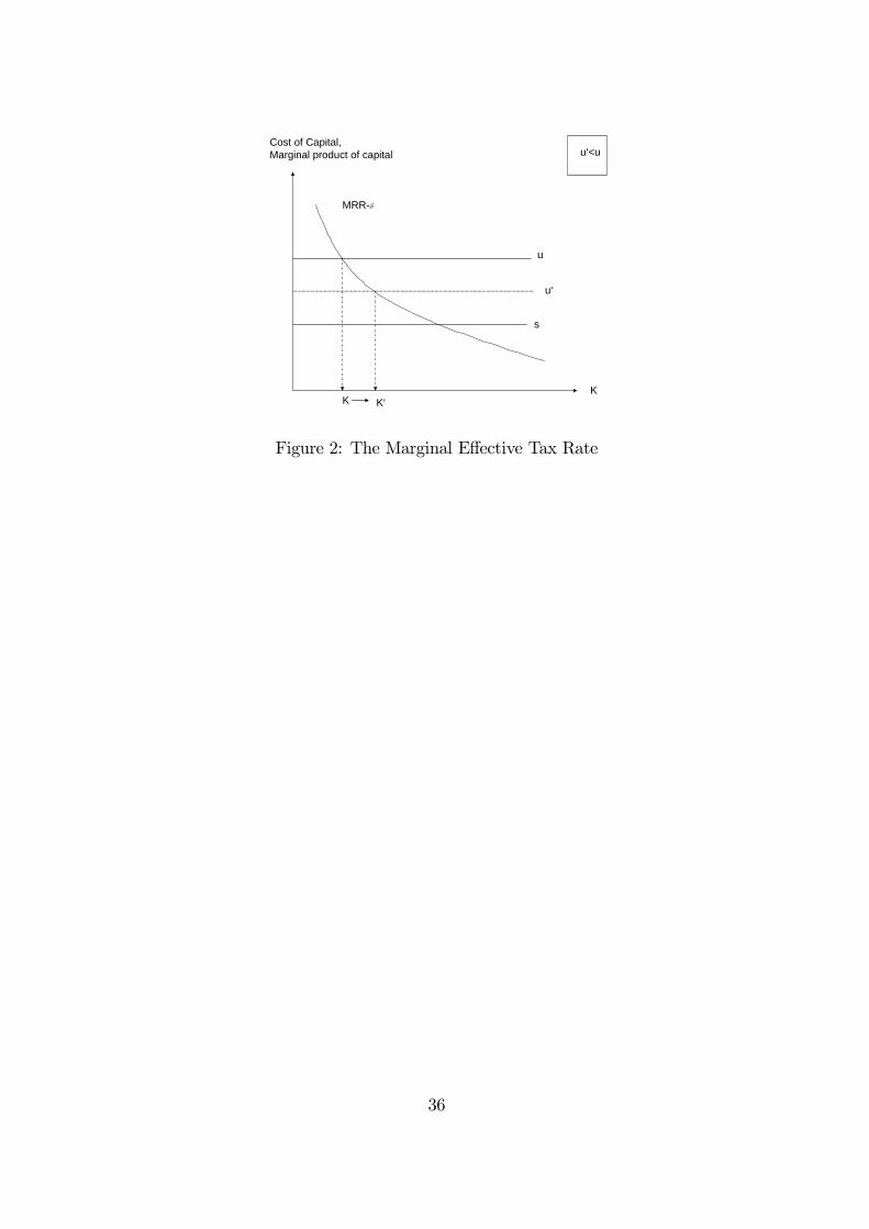
The marginal effective tax rate is defined as the difference between the pre-tax return of

the corporation, denoted by u (= cost of capital as given in (17)), and the after-tax return

to the investor, denoted by s = (1 − ti)i. This marginal effective tax rate measures the

overall distortion of taxation with respect to investment incentives. It is straightforward

that taxes at the corporate and personal level drive a wedge between the required pre-tax

return u and the net of tax return s to households. Using once again equation (17) we

can define the cost of capital as:

u = Marginal Rate of Return − δ,

= FK − δ +m0b2.

The marginal effective tax rate is defined as the difference between the cost of capital

and the net of tax return to the private investor divided by the cost of capital, teff = u−su.

Under the present German tax system, the cost of capital amount to about 4.7 per cent and

the after tax return for a representative investor is approximately 3.0 per cent, implying

an effective marginal tax rate of about 36.4 per cent.

Figure 2 here

Given decreasing returns to capital, the marginal rate of return curve will slope down-

ward as shown in Figure 2. In a world without taxation, the cost of capital, u, equals the

after-tax return to private investors, s. Thus, the intersection of both curves denotes the

long-run capital stock in the absence of taxation. However, the corporate income tax at

the firm level and the dividend and capital gains taxes at the personal level increase the

19

cost of capital and thus have a negative effect on capital accumulation. For example, the

proposed DIT reform diminishes the tax wedge by eliminating the dividend and the cap-

ital gains tax and by reducing the profit tax rate. In turn the cost of capital, u, declines

to u0 and thus the distance to the after tax return to savers, s, dwindles and stimulates

therefore the capital accumulation in the economy.

3.2 Households and General Equilibrium

Since we mainly focus on the welfare implications rather than on the distributional issues

we model the household sector using the Ramsey model of an infinitely lived household.

This representative agent takes the discounted utility of all future generations into ac-

count, where the subjective discount factor is denoted by ρ < 1. Accordingly, households

maximize life time utility:

Ut = u©Ct − ϕ(LS

t )ª+ ρ · Ut+1 =

∞Ps=t

ρs−t · u©Ct − ϕ(LS

t )ª, (18)

subject to their budget constraint:

GAt+1 = (1 + rt)At + (1− tL)wtLst + tL · LTA+ TH

t − (1 + tC)Ct . (19)

Utility depends on individual consumption Ct less the disutility of work, ϕ(LSt ), where

LSt expresses labour supply.

14 Households face a trade-off between the utility stemming

from consumption and the disutility of work, implying an endogenous labour supply in the

model. Household’s budget consists of interest bearing financial assets, (1 + rt)At, net of

tax labor income, (1−tL)wtLSt +t

L ·LTA, where LTA stands for a labour tax allowance on14This special form is chosen since we are only interested in the substitution effect and not

the income effect.

20

houseold level, and governmental lump sum transfers THt . Wealth accumulates according

to income inflow, net of consumption expenditures, (1 + tC)Ct.

Solving the maximization problem of the household, optimal individual labor supply

is determined by the current real wage:

ϕ0(LSt ) =

(1− tL)

(1 + tC)wt . (20)

As one can easily see, an increase in the labour tax, tL, as well as an increase in the VAT,

tC , will lead to a decrease in labour supply: ∂ϕ0(LSt )∂tL

< 0 and ∂ϕ0(LSt )∂tC

< 0. According to the

reform proposal, the labour tax will be decreased, while the VAT tax is raised in order to

finance the DIT reform to assure a balanced governmental budget.

Deriving the Euler equation of consumption:

u0£Ct − ϕ(LS

t )¤

u0£Ct+1 − ϕ(LS

t+1)¤ = 1 + tCt

1 + tCt+1

ρ(1 + rt+1)

G. (21)

we can analyze how a change in the VAT rate affects future consumption and therefore

the savings behavior of domestic households. A rise in the VAT rate leads to a decline

in expected future income and thus current consumption is reduced and savings increase.

Moreover, the decline in the net interest rate which results from the increase in the interest

tax also encourages savings through the income effect, since people save more given the

lower return on savings, to attain a given level of savings in the future. However, there is

only a temporary change in the net interest rate since in the long run the interest rate is

bound to fulfill 1 + r = ρ/G due to the assumptions underlying the Ramsey model.

As a measure of welfare, we apply the equivalent variation, which specifies the differ-

ences in expenditures with respect to the before and after tax reform utility levels U0 and

21

U1, using the pre reform price structure p0:

EV = TW (U1, p0)− TW (U0, p0) . (22)

Summing up all single differences in expenditures for each period and comparing the

present value of this stream to GDP or life-time income, we can compute the change in

welfare in per cent of GDP, or life-time income, respectively.

The Rest of the World (ROW) is assumed to be a representative foreign agent who

closes the model. ROW is endowed with an exogenous income stream and chooses an

optimal consumption stream to maximize life time utility. Moreover, ROW can only save

in terms of the internationally traded bonds. However, domestic investment does not stem

solely from domestic sources but also from foreign savings, resulting in a current account

deficit or surplus depending on the policy experiment. The current account is given by:

GDFt+1 −DF

t = rtDFt + TBt , (23)

where DFt denotes foreign government debt and TBt the domestic trade balance. Since

we applied the source principle of interest taxation, a decrease in the domestic net interest

rate also affects foreign savings, however, since the the net interest rate is fixed due to

the assumptions underlying the Ramsey model, there is almost no change in the amount

of foreign government bonds held by domestic individuals.

4 Policy Scenarios & Simulation Results

Starting from the prevailing German tax system in 2003, the statutory corporate tax

rate amounts to 25 per cent but adding the local trade tax and the solidarity surcharge

22

the effective corporate tax rate adds up to 38.6 per cent. On the household level, the

progressive labour tax rate reaches a top marginal tax rate of 48.5 per cent, including the

solidarity surcharge it amounts to 51.2 per cent. Taking an average annual income of about

20,814 per year as given, the representative agent, according to the prevailing tax bracket,

is liable to a marginal income tax of 28 per cent, which if we add the solidarity surcharge,

reaches 29.5 per cent . This tax rate also applies to interest income. According to the

German half income principle, income stemming from dividends (distributed profits) is

subject to half of the personal income tax rate, while capital gains are untaxed.

In the following we consider three different policy scenarios: Scenario 1 takes the

reform proposal made by the GCEA in their 2003 report. All tax rates applying to

any kind of capital income are set at a flat rate of 30 per cent while labour income is

taxed progressively with a top marginal tax rate of 35 per cent.15 Again, we do not

use the top marginal labour tax rate but compute the marginal income tax rate of an

average individual which would amount to approximately 24 per cent. To avoid any

double taxation of distributed profits the full imputation system is installed, implying a

dividend tax rate of zero. Since no capital losses should be regarded, capital gains also

need to be tax exempt, implying a capital gains tax rate of zero.

Scenario 2 takes advantage of the ‘New View’ setting. As discussed above, the divi-

dend tax is supposed to be neutral along the “New View” and therefore the dividend tax

has no impact on the investment decision of firms. Accordingly, Scenario 2 is identical to

Scenario 1, but the dividend tax is set at a flat rate of 30 per cent. In this model, the

15The current local trade tax, the German ‘Gewerbesteuer’has been abolished in its existingform as an additional charge, and is embedded in the capital and labour income tax rate,respectively.

23

dividend tax is a well-suited, non-distorting instrument to raise additional tax revenue.

Last but not least, Scenario 3 represents the “pure” dual income tax system, suggest-

ing that all kinds of capital income are taxed at a flat rate. Thus, dividends will also be

subject to taxation at a flat rate of 30 per cent. Since capital gains are only taxable upon

realization and not on the accrual basis we take half of the proposed statutory tax ( that

is 15 per cent) rate as a rule of thumb in the simulation exercise.

Table 1 here

The column "Status Quo" depicts the effective tax rates for Germany in the year 2003,

while the other three columns show the effective tax rates referring to the simulation

exercises of scenario one to three. Regarding the major loss in tax revenue — which will

arise due to the large reduction in several tax rates, there are only very few feasible ways

to finance the reform. TheGCEA report proposes a comprehensive reduction of nearly all

legal tax reliefs but it is arguable whether this counteracting measure is sufficient. Since

the tax revenue is determined endogenously in our model, we allow for an increase in the

VAT rate to finance the proposed reform scenarios. Moreover, the increase in the VAT

rate is the preferred alternative by political analysts in finding ways to finance different

tax reforms (Fehr and Wiegard, 2004).

4.1 Behavioral Parameters

Relying on the comparative static analysis performed in chapter 3.1.4., we anticipate

that the first two proposed reform scenarios will have a stimulating effect on capital

24

accumulation and therefore on economic growth. However, this kind of examination only

gives qualitative insights of the policy proposals. To achieve quantitative results, we apply

a CGE model calibrated to a stationary equilibrium along a balanced growth path of the

German economy. The real growth rate of the German economy is approximated to be

1 per cent, which is a quite fair estimation for Germany after re-unification. Economic

depreciation is assumed to be 10 per cent and the adjustment speed towards the new

steady state is determined by the half life of investments. Following the study of Cummins

et al. (1996) we take a value of 8.0, implying that during the following 8 years after the

policy shock half of the long run increase in the capital stock is accumulated. Accordingly,

99.9 per cent of the new steady state capital stock will be built up within 80 years.

Since the simulation results of any CGE model are strongly sensitive towards the

behavioral parameters applied, special diligence is needed when calibrating the model. All

behavioral parameters used in this model are standard results confirmed by the empirical

literature. The most important ones are summarized here in Table 2:

Table 2 here

The elasticity of capital demand can be interpreted as follows: A one percent increase

in the cost of capital leads to a decline in the long-run capital stock by one percent.

Concerning the elasticity of the debt-asset ratio, a decrease in the profit tax rate by

8.3 percentage points (so from the present 38.3 per cent to the suggested 30 per cent),

will lead to an increase in the debt asset ratio of 0.36∗8.6 = 3.96 percentage points.

The labour supply elasticity, representing an average over empirical estimates for dif-

ferent age and sex groups, is actually a compensated supply elasticity, thus showing just

25

the substitution effect between labour and leisure since this is the only effect we are

interested in.

4.2 Quantitative Results

The reform proposal is characterized by a large reduction of corporate and personal tax

rates. Due to the reduction in the corporate tax rate, as well as the nonexistence of

a dividend and capital gains tax, the cost of capital decreases by about nine per cent

from 4.7 to 4.3 per cent in Scenario 1, as shown in Table 3. In Scenario 2, the cost of

capital declines only by seven per cent since in this case a dividend tax is also levied.

This considerable decline in the cost of capital goes hand in hand with a reduction of the

marginal effective tax rates thus boosting investments and enhancing economic growth.

The marginal effective tax rate16 declines by 17 per cent from 36.4 to 30.2 per cent in

Scenario 1 and by 13 per cent in Scenario 2. The capital stock increases from its initial

value by about 5.8 per cent in Scenario 1 and by 5.4 per cent in Scenario 2 leading in

turn to an increase in GDP by 3.3 and 3.5 per cent, respectively. Similar results are also

produced by the simulation model of Fehr andWiegard (2004). Concerning Scenario

3, the increase in the interest tax rate decreases the cost of equity finance on the one hand.

However, on the other hand, the introduction of the capital gains tax of 15 per cent works

in the opposite direction and raises the cost of equity finance. This result derives from the

fact that we model the new view of dividend taxation and consider marginal investments

to be financed via retained earnings. Thus, the increase in the capital gains tax leads to

16The marginal effective tax rate is defined as the difference between the pre-tax return of thecorporation and the investor’s after tax return divided by the cost of capital.

26

a rise in the cost of capital by around two per cent .

Table 3 here

We start each simulation scenario from a calibrated equilibrium, where 55 per cent of

net investments are financed via retained earnings and 40 per cent via debt. New share

issues are fixed at a rate of 5 per cent and do not vary over time. In Scenarios 1 and 2,

the effect caused by the slight increase in the interest tax rate as well as by the lowering

of the corporate tax rate, leads to a rise in the relevance of retained earnings as a source

of finance. In the new long run equilibrium 58 instead of 55 per cent of net investments

are financed via retained earnings. Concerning debt as a source of finance, only 37 per

cent of overall (net) investments are financed via debt as compared to 40 per cent before

the reform. Summarizing, in Scenarios 1 and 2 equity is more intensively used as a source

of finance thus leading to a strengthening of the equity position of the representative firm

and lowering the indebtedness in the new steady state. The debt asset ratio decreases by

7.6 per cent in both cases. In Scenario 3 we observe a slight increase in the debt asset

ratio of 0.9 per cent. This effect arises, since the introduction of the capital gains tax

increases the price of equity compared to debt as a source of finance.

Table 3 provides a rough overview of further important long-run, key economic figures

on the household side. Until now, the simulation results of Scenarios 1 and 2 did not

differ noticeably, thus the results concerning the change in domestic assets may surprise

at first glance. The explanation is intuitive: While there is no dividend tax in Scenario

1, firm values — which represent a major share (ca. 38 per cent) of the financial wealth of

households — increase due to reform Scenario 1 by 27 per cent. In contrast, in Scenario 2,

27

where a dividend tax of 30 per cent is levied, the firm value decreases by eight per cent

from its initial value. Thus, the change in firm values influences the change in the asset

position significantly.

On the household level the reform is characterized by a major reduction in the personal

income tax rates. For an average individual the marginal labour income tax rate drops

from 29.4 to 24 per cent. This tax relief has a major impact on the labour-leisure decision

and households are willing to supply a larger amount of labour to the firm sector. The

increased investment and capital accumulation lead also to a rise in wages of 1.4 and 1.1

per cent in Scenario 1 and 2 respectively. This result derives from the fact that capital and

labour are complementary production factors and accordingly an increased capital stock

increases the demand for labour. In turn, households increase their labour supply by 2.2

and 2.6 per cent in Scenarios 1 and 2. The larger increase in labour supply in the second

case must be astonishing at first glance. Even though gross wages increase more in the

first Scenario, it is current real wages, which also depend on consumption taxes, that affect

the supply of labour by households. Since the VAT rate increases by only two percentage

points in the second Scenario (compared to 3.7 percentage points in Scenario1), it is clear

that labour supply will be higher as a result of this second alternative reform proposal.

However, this is not the only effect that determines labour supply. Due to the aug-

mented capital accumulation, the marginal product of labor — the complementary produc-

tion factor — rises, also implying an increase in labour supply . Thus, disposable income

of households increases by seven per cent in Scenario 1 and by 7.6 per cent in Scenario 2

leading to a rise in consumption of 2.8 and 3.3 per cent, respectively.

28

Since the reform scenarios have to be financed somehow, we allow for the VAT to

adapt in order to balance the governmental budget without cutting lump-sum transfers

to households. Simulating Scenario 1, the VAT increases from initially 16 per cent by 3.7

percentage points to 19.7 per cent assuring that the reform is revenue neutral. Since the

government can draw on an additional tax revenue from the dividend taxation in Scenario

2, the required increase in the VAT rate amounts to only 2 percentage points, thus nearly

2 percentage points less than in Scenario 1. In Scenario 3, the VAT rate also rises to a

level of about 18 per cent. The increase in revenue from capital gains taxation is not large

enough to balance the governmental budget such that the VAT has to adjust accordingly

to make the reform revenue neutral.

To be able to evaluate the welfare implications17 of the three reform scenarios we

rely on the equivalent variation to measure welfare. Therefore, we compute pre and post

reform utility levels of a representative individual and calculate how much money the

agent would need before the reform to reach the same utility level that is achieved after

the reform. The present value of this cash flow is then expressed in terms of total life-

time income of the representative agent and GDP. Scenario 2 yields not only the largest

increase in GDP but also the largest increase in welfare. While welfare in terms of life-

time income increases by 1.7 per cent — which is equivalent to a 0.9 per cent increase in

terms of GDP — in Scenario 2, in Scenario 1, welfare only amounts to 0.8 per cent of GDP

. The lowest increase in welfare in Scenario 3 is basically the result of the high capital

gains taxation, which leads to a weaker increase in disposable income and consumption.

17Welfare is measured without public services.

29

4.3 Sensitivity Analysis

The large number of empirical papers that estimate different values for important be-

havioral parameters used in the model suggests to check the robustness of our results if

different values for the key behavioral parameters are assumed. There are basically four

different elasticities which are of interest in our context: The labour supply elasticity ε,

the intertemporal elasticity of substitution σC, the elasticity of factor substitution σK ,

and the elasticity concerning the debt asset ratio σB .

Table 4 here

Tables 4, 5 and 6 show the results of the simulation exercise of Scenarios 1, 2 and

3, respectively, with different values for the underlying elasticities. The basic scenario

applies a labour supply elasticity of ε = 0.37 which is a weighted average of compensated

wage elasticities of labour supply for Germany estimated by Fenge et al. (2002).18

If we set this elasticity close to zero, i.e. to ε = 0.01, we model an almost fixed labour

supply. 19 Simulating scenario 1 (2, 3), the labour supply increases by only 0.05 per

cent (0.06 per cent, 0.05 per cent) and thus also capital accumulation is impeded. In the

long run the capital stock increases by only 3.58 per cent (2.81 per cent) instead of the

5.76 per cent (5.43 per cent) calculated in the base Scenario 1 (2). Accordingly, private

consumption increases only to a smaller extent of 0.28 (0.27) per cent.

18The authors compute four different elasticities for men and women aged 20-39 and 40-39,using data from the German Socio-Economic Panel We then compute a weighted average of0.37, using these elasticities and the share of employed in each of these categories.19Such an assumption is plausible for Germany, as shown by the last tax reform : Although the

German Tax Reform 2000 lead to a significant decrease in personal income tax rates employmentdid not increase, but decreased due to labor market rigidities and various other structuralproblems (Sinn 2004).

30

Table 5 here

Next, the values of the intertemporal elasticity of substitution, σC , reflect the change

in the pattern of consumption and saving over time. We start with a value of 0.4 in the

base scenario and then run the simulation with a higher value of 0.6. The model is to

a large degree robust to the change in the intertemporal elasticity of substitution. The

results change only slightly as depicted in the fourth column of tables 4 through 6. The

reason why the results do change only so little is due to the fact that the long-run interest

rate is bound to equal the rate of time preference in the long-run in the Ramsey model

and the difference in tax rates on interest income before and after the reform is negligible.

20

Table 6 here

Another important parameter is the elasticity of substitution between capital and

labour. This elasticity is like a capital demand elasticity in our model. The more elastic

capital demand is, the higher is the reaction to a change in the tax rates. Accordingly,

even a slight lowering of the pre-tax rate of return will stimulate capital creation. A

higher elasticity means that in Figure 2 the MRR curve becomes flatter such that at a

given pre-tax rate of return s the same decrease in the required pre-tax rate of return20Still, the following effects can arise as a result of a change in the taxation of interest income.

According to theory, a higher intertemporal elasticity will have a stronger effect on the savingsbehavior of households. If the net interest rate decreases, savings will increase, since the incomeeffect will dominate the substitution effect. The substitution effect arises since a lower interestrate increases the price of future periods consumption and thus we have a substitution of presentconsumption for future consumption. However, a lower interest rate leads to a positive incomeeffect since the amount of savings needed to attain a given consumption level tomorrow, isincreased.

31

u is followed by a higher adjustment of the capital stock. The basic scenario employs

a factor substitution elasticity of the CES production function of 0.8. There are several

estimates for this measure in the empirical literature, thus we simulate the proposed

scenarios with a higher elasticity of 1.3. The higher elasticity leads to an even larger

increase in the change of the long run capital stock compared to the base case. The long

run capital stock increases by 8.15 (7.31) per cent in Scenario 1 (2) and only by 0.9 per

cent in Scenario 3. Accordingly, the increased capital intensity leads to a change in labour

supply, which increases by 2.21 per cent and 2.66 per cent in Scenarios 1 and 2. In turn,

the consumption level of households rises by about three and 3.5 per cent, respectively.

Regarding the debt elasticity, this measure shows how elastic the firm’s debt ratio

reacts to different tax reform scenarios. In the baseline model the elasticity concerning

the debt asset ratio is set to 0.36, while column six and seven of Tables 4 through 6

show the simulation results using a debt asset elasticity of 0.16 and 0.56, respectively.

Firms choose the optimal debt level such that the costs of internal financing and external

financing are equalized. If internal financing becomes cheaper, i.e. the required rate of

return declines, enterprises will start financing more of their investments via retained

earnings until the costs of external financing also decline due to the shrinking debt ratio.

A reduced elasticity of e.g. 0.16 leads to a less elastic reaction of firms to cheaper internal

financing.

32

5 Conclusion

Following the ongoing discussion of reforming the German tax system, the paper takes

up the reform proposal made by the German Council of Economic Advisors in

2003. This reform proposal suggests a dual income tax for Germany similar to the one

already practiced in the Nordic Countries. To analyze the economic effects of such a

dual tax system, we apply a dynamic computable general equilibrium model and simulate

three different reform scenarios. With standard assumptions on behavioral parameters

and marginal tax rates, the reform leads to an increase in investments and therefore in

capital accumulation of about 5.8 per cent. Comparing steady state values, GDP rises by

3.3 per cent and household consumption by 2.8 per cent. This complete restructuring of

the tax system leads in the long run to a welfare gain of approximately 0.8 per cent of

GDP which is mainly based on the increase in life-time wealth as a result of the lower tax

burden. These results are to a large extent robust concerning the choice of the behavioral

elasticities. The only important exemption is the labor supply elasticity. If we assume

a labor supply elasticity close to zero, which is quite plausible for Germany due to the

current frictions on the German labor market, the growth impact of this comprehensive

tax reform diminishes. For example, the capital stock increases by only 3.9 per cent

instead of the initial 5.8 per cent and GDP rises by only 1.2 per cent instead of the former

3.3 per cent. Thus, the labour supply is an important determinant of growth in two

respects: First, if a tax reform stimulates capital accumulation a lack of labour supply

will impede the accumulation of the complementary production factor capital. Second, if

labour supply does not respond to tax incentives, households can not earn any additional

33

income and thus there is no demand side driven growth.

Thus, the change from the prevailing comprehensive income tax system to a dual

income tax system will have a significant impact on capital accumulation and growth as

well as on households’ welfare, particularly if the economy has a well functioning labor

market.

34

it(1-ti)/(1-tg)

m+bm‘

bb*

it(1-ti)/( 1-tg1)

b*1

it(1-ti1)/(1-tg)

b*2

tg1>tgti1>ti

Cost of debt,Cost of equity

Figure 1: The Optimal Debt/Asset Ratio

35

K

MRR-δ

s

u

u‘

K K‘

u‘<uCost of Capital,Marginal product of capital

Figure 2: The Marginal Effective Tax Rate

36

Table 1: Tax Rates Before and After the ReformStatus Quo (2003) Scenario 1 Scenario 2 Scenario 3

Profit Tax, tU 0.386 0.30 0.30 0.30Labour Tax, tL 0.295 0.24 0.24 0.24Tax on Interest Income, ti 0.295 0.30 0.30 0.30Dividend Tax, tD 0.148 0.00 0.30 0.30Capital Gains Tax, tG 0.00 0.00 0.00 0.15VAT, tC 0.16 endogenous endogenous endogenousSource: Ministry of Finance, (BMF, 2004), (GCEA, 2003)

37

Table 2: Behavioral Parameter ValuesElasticity of Capital Demand∗) (CHIRINKO 2002) - 1.0Half Life of Capital Accumulation (in years) (CUMMINS et al. 1996) 8.0Elasticity of Debt-Asset Ratioˆ) (GRAHAM et al. 1998) 0.36Intertemporal Elasticity of Substitution (FLAIG 1988) 0.4Elasticity of Factor Substitution (GERMAN BUNDESBANK 1995) 0.8Labour supply elasticity (weighted average of FENGE et al. 2002) 0.37Elasticity with respect to: ∗) cost of capital; ˆ) profit tax

38

Table 3: Key Economic Figures (Long Run Change in %)Scenario 1 Scenario 2 Scenario 3

Capital stock 5.8 5.4 1.4Cost of Capital - 8.9 - 6.9 1.9Marginal Effective Tax Rate - 17.1 - 13.0 3.2Gross Domestic Product 3.3 3.5 1.9Equity as Source of Finance 5.5 5.5 - 0.6Debt Asset Ratio - 7.6 - 7.6 0.9Domestic Assets 4.8 - 8.5 -1.8Gross Wage 1.4 1.1 -0.3Labour Supply 2.2 2.6 2.1Disposable Income 7 7.6 5.6Domestic Consumption 2.8 3.3 2.5VAT Rate (Change in %-points) 3.7 2 1.9Welfare in % of Life Time Income 1.4 1.7 1.2Welfare in % of GDP 0.8 0.9 0.6Source: own calculations

39

Table 4: Sensitivity Analysis (Long Run Changes in %)Scenario 1 ∗) ε = 0.01 σC = 0.6 σK = 1.3 σB = 0.16 σB = 0.56

Change in capital stock 5.75 3.58 5.76 8.15 5.70 5.80Change in stock of debt - 2.34 - 4.31 - 2.29 - 0.08 2.11 - 6.70Change in labour supply 2.15 0.05 2.15 2.21 2.14 2.16Change in onsumption 2.80 0.28 2.80 2.95 2.75 2.83∗)applied parameters: ε = 0.37; σC= 0.4; σK = 0.8; σB = 0.36;Source: own calculations.

40

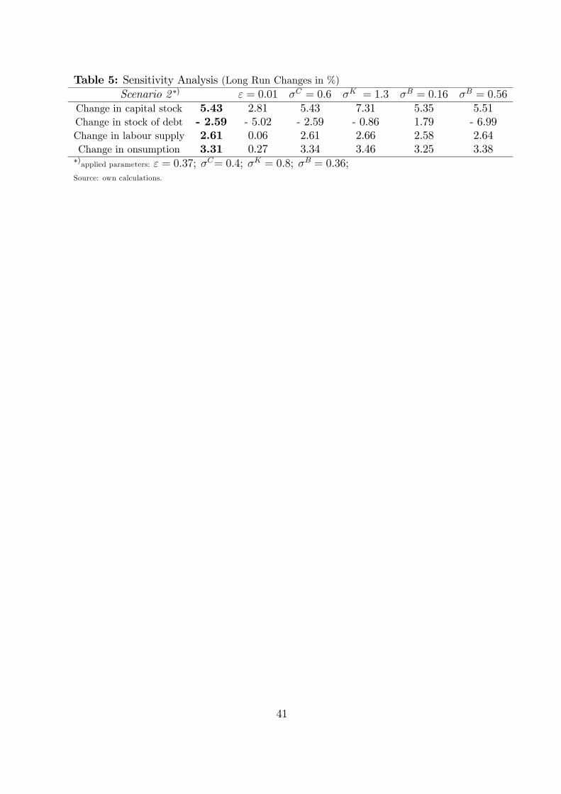
Table 5: Sensitivity Analysis (Long Run Changes in %)Scenario 2 ∗) ε = 0.01 σC = 0.6 σK = 1.3 σB = 0.16 σB = 0.56

Change in capital stock 5.43 2.81 5.43 7.31 5.35 5.51Change in stock of debt - 2.59 - 5.02 - 2.59 - 0.86 1.79 - 6.99Change in labour supply 2.61 0.06 2.61 2.66 2.58 2.64Change in onsumption 3.31 0.27 3.34 3.46 3.25 3.38∗)applied parameters: ε = 0.37; σC= 0.4; σK = 0.8; σB = 0.36;Source: own calculations.

41

Table 6: Sensitivity Analysis (Long Run Changes in %)Scenario 3 ∗) ε = 0.01 σC = 0.6 σK = 1.3 σB = 0.16 σB = 0.56

Change in capital stock 1.36 - 0.67 1.36 0.90 1.37 1.36Change in stock of debt 2.23 0.18 2.23 1.76 1.75 2.71Change in labour supply 2.09 0.05 2.09 2.08 2.09 2.09Change in onsumption 2.48 0.00 2.48 2.44 2.49 2.47∗)applied parameters: ε = 0.37; σC= 0.4; σK = 0.8; σB = 0.36; σB = 0.36Source: own calculations.

42

Acknowledgement 1 The authors are particularly grateful for the comprehensive sup-

port by Christian Keuschnigg concerning the theoretical underpinning as well as the nu-

merical implementation of the model. Further we would like to thank Bernd Genser, Soren

Bo Nielsen, Assaf Razin, Hans-Werner Sinn, Christian Valenduc and Wolfgang Wiegard

for the helpful discussions and insightful comments. The paper was presented at a num-

ber of conferences in 2004 including the IIPF Conference, Milan, CESifo Venice Summer

Institute, EARIE Conference, Berlin, CGEMod, Brussels and seminars at the University

of Munich, Konstanz and Tel Aviv.

43

References

[1] Auerbach, Alan J. 2002. Taxation and Corporate Financial Policy, In: Auerbach,A., Feldstein, M. (eds.), Handbook of Public Economics, Vol. 3. North-Holland,Amsterdam: Elsevier, pp. 1251-1292.

[2] Auerbach, A. J., Hassett, K. A. 2003. On the Marginal Source of InvestmentFunds. Journal of Public Economics 87, 205-232.

[3] BMF 2004, Ministry of Finance, http://www.bundesfinanzministerium.de/Anlage24285/Grafische-Uebersichten.pdf, found 02.08.2004.

[4] Boadway, R. 2004. The Dual Income Tax System - An Overview. CESifo DiceReport Vol. 2, No. 3, 3-8.

[5] Chirinko, R. S. 2002. Corporate taxation, Capital Formation, and the SubstitutionElasticity Between Labor and Capita. CESifo Working Paper No. 707.

[6] Cnossen, S. 2000. Taxing Capital Income in the Nordic Countries: a model for theEuropean Union? In: Taxing Capital Income in the European Union - Issues andOptions for Reform. S. Cnossen (Ed.). Oxford University Press.pp. 181-213

[7] Cummins, J. G., K. A. Hassett, G. R. Hubbard ,1996. Tax Reform and Invest-ment: A Cross-Country Comparison. Journal of Public Economics 62, 237-273.

[8] Devereux, M., R.Griffith, A.Klemm 2002. Corporate Income Tax Reforms andInternational Tax Competition. Economic Policy, 35, 449-495.

[9] Diamond, P. A and J. A. Mirrlees, 1971, Optimal Taxation and Public Produc-tion: I—Production Efficiency, American Economic Review 61, 8-27.

[10] Dietz, M., C. Keuschnigg, 2004, Corporate Income Tax Reform in SwitzerlandSwiss Journal of Economics and Statistics, forthcoming.

[11] Dietz, M., C. Keuschnigg, 2003. Unternehmenssteuerreform II, QuantitativeAuswirkungen auf Wachstum und Verteilung. Schriftenreihe “Finanzwirtschaft undFinanzrecht”, Haupt Verlag, Bern.

[12] European Commission, 2001, Company Taxation in the Internal Market, Com-mission StaffWorking Paper, COM (2001) 582 final.

[13] Fehr, H. 1999. Welfare Effects of Dynamic Tax Reforms, Mohr-Siebeck.

[14] Fehr, H., W. Wiegard, 2004. Abgeltungssteuer, Duale ESt und zinsbereinigteESt: Steuerreform aus einem Guss. In Dirrigl, H., D. Wellisch, E. Wenger (Eds.).Steuern, Rechnungslegung und Kapitalmarkt: Festschrift für Franz W. Wagner zum60. Geburtstag. Wiesbaden, pp. 27-43.

[15] Fenge, R., S. Übelmesser, M.Werding, 2002. Second-Best Properties of ImplicitSocial Security Taxes: Theory and Evidence, CESifo Working Paper No. 743.

44

[16] Gordon, R. H., Y. Lee, 2001, Do Taxes Affect Corporate Debt Policy? Evidencefrom US Corporate Tax Return Data, Journal of Public Economics 81, 195-224.

[17] International Bureau of Fiscal Documentation 2004. European Tax Handbook 2004,Amsterdam.

[18] King, M. A., D. Fullerton, 1984. The Taxation of Income from Capital, Chicago.

[19] Keuschnigg, C., 2002. Analyzing Capital Income Tax ReformWith a CGE GrowthModel for Switzerland. Technical Report, Institut für Finanzwissenschaft und Fi-nanzrecht der Universität St. Gallen.

[20] Keuschnigg, C., 1991, The Transition to a Cash Flow Income Tax, Swiss Journalof Economics and Statistics 127, 113-140.

[21] Laxton, D., P. Isard, H. Faruqee, E. Prasad, B.Turtelboom ,1998. MULTI-MOD Mark III: The Core Dynamic and Steady-State Models, Occasional Paper 164,International Monetary Fund. Washigton D.C.

[22] Mendoza, E. G., A. Razin, L. L.Tesar, 1994. Effective Tax Rates in Macroeco-nomics: Cross-country estimates of tax rates on factor incomes and consumption,Journal of Monetary Economics 34. 297-323.

[23] Mennel A., J. Förster 2003, Steuern, 49. Lieferung 2003, Strömberg/Alhager.

[24] Norwegian Ministry of Finance 2004, http://odin.dep.no.fin/engelsk/p4500279/p30004927/index-b-f-a.html.

[25] Sachverständigenrat zur Begutachtung der gesamtwirtschaftlichen Entwick-löung -German Council of Economic Experts 2003, Jahresgutachten 2003/04,Wiesbaden.

[26] Sinn, H.-W. , 2004. Ist Deutschland noch zu retten?, Berlin: Econ Verlag.

[27] Sinn, H.-W., 1991. The Vanishing Harberger Triangle, Journal of Public Economics45. 271-300.

[28] Sinn, H.-W., 1987. Capital Income Taxation and Resource Allocation, Amsterdam:North-Holland.

[29] Sinn, H.-W., 1981. Capital Income Taxation, Depreciation Allowances and Eco-nomic Growth: A Perfect-Foresight General Equilibrium Model, Zeitschrift für Na-tionalökonomie 41. 295-305.

[30] Sørensen, P. B., 2001. The Nordic Dual Income Tax - In or Out?, invited speechdelivered at the meeting of the Working Party 2 on Fiscal Affairs, OECD, 14 June2001.

[31] Sørensen, P. B. ,2001. OECDTAX: A Model of Tax Policy in the OECD Economy,Technical Working Paper, University of Copenhagen.

45

[32] Sørensen, P. B., 2000. The Case for International Tax Coordination Reconsidered,Economic Policy 31, pp. 429-461.

[33] Sørensen, P. B.,1994. From the Global Income Tax to the Dual Income Tax: RecentTax Reforms in the Nordic Countries, International Tax and Public Finance 1. 57-79

[34] Statistisches Bundesamt 2003, Statistische Jahrbuch 2003 für die Bundesrepub-lik Deutschland, Wiesbaden.

[35] Strulik, H., 2003. Supply-Side Economics of Germany’s Year 2000 Tax Reform: AQuantitative Assessment, in German Economic Review 4. 183-202.

[36] Wagner, F. W. 2000. Korrektur des Einkünftedualismus durch Tarifdualismus -Zum Konstruktionsprinzip der Dual Income Taxation, Steuern und Wirtschaft 4.431-441.

46

Ifo Working Papers No. 19 Osterkamp, R. and O. Röhn, Being on Sick Leave – Possible Explanations for Differ-

ences of Sick-leave Days Across Countries, November 2005. No. 18 Kuhlmann, A., Privatization Incentives – A Wage Bargaining Approach, November

2005. No. 17 Schütz, G. und L. Wößmann, Chancengleichheit im Schulsystem: Internationale deskrip-

tive Evidenz und mögliche Bestimmungsfaktoren, Oktober 2005. No. 16 Wößmann, L., Ursachen der PISA-Ergebnisse: Untersuchungen auf Basis der internatio-

nalen Mikrodaten, August 2005. No. 15 Flaig, G. and H. Rottmann, Labour Market Institutions and Employment Thresholds. An

International Comparison, August 2005. No. 14 Hülsewig, O., E. Mayer and T. Wollmershäuser, Bank Loan Supply and Monetary

Transmission in Germany: An Assessment Based on Matching Impulse Responses, Au-gust 2005.

No. 13 Abberger, K., The Use of Qualitative Business Tendency Surveys for Forecasting Busi-

ness Investing in Germany, June 2005. No. 12 Thum, M. Korruption und Schattenwirtschaft, Juni 2005. No. 11 Abberger, K., Qualitative Business Surveys and the Assessment of Employment – A

Case Study for Germany, June 2005. No. 10 Berlemann, M. and F. Nelson, Forecasting Inflation via Experimental Stock Markets:

Some Results from Pilot Markets, June 2005. No. 9 Henzel, S. and T. Wollmershäuser, An Alternative to the Carlson-Parkin Method for the

Quantification of Qualitative Inflation Expectations: Evidence from the Ifo World Eco-nomic Survey, June 2005.

No. 8 Fuchs, Th. and L. Wößmann, Computers and Student Learning: Bivariate and Multivari-ate Evidence on the Availability and Use of Computers at Home and at School, May 2005.

No. 7 Werding, M., Survivor Benefits and the Gender Tax-Gap in Public Pension Schemes –

Work Incentives and Options for Reform, May 2005. No. 6 Holzner, Chr., Search Frictions, Credit Constraints and Firm Financed General Training,

May 2005. No. 5 Sülzle, K., Duopolistic Competition between Independent and Collaborative Business-to-

Business Marketplaces, March 2005. No. 4 Becker, Sascha O., K. Ekholm, R. Jäckle and M.-A. Muendler, Location Choice and Em-

ployment Decisions: A Comparison of German and Swedish Multinationals, March 2005. No. 3 Bandholz, H., New Composite Leading Indicators for Hungary and Poland, March 2005. No. 2 Eggert, W. and M. Kolmar, Contests with Size Effects, January 2005. No. 1 Hanushek, E. and L. Wößmann, Does Educational Tracking Affect Performance and Ine-

quality? Differences-in-Differences Evidence across Countries, January 2005.