Implementation of Weigh-in-Motion (WIM) Systems · that good data can be useful for bridge...

Implementation of Weigh-in-Motion (WIM) Systems

FINAL REPORT February 2009

Submitted by

NJDOT Research Project Manager W. Lad Szalaj

FHWA-NJ-2009-001

In cooperation with

New Jersey Department of Transportation

Bureau of Research and

U.S. Department of Transportation Federal Highway Administration

Dr. Ali Maher* Director and Professor

Dr. Patrick J. Szary* Research Engineer

*Center for Advanced Infrastructure & Transportation (CAIT) Rutgers, The State University

100 Brett Road Piscataway, NJ 08854-8014

Disclaimer Statement

"The contents of this report reflect the views of the author(s) who is (are) responsible for the facts and the accuracy of the data presented herein. The contents do

not necessarily reflect the official views or policies of the New Jersey Department of Transportation or the Federal Highway Administration. This report does not constitute

a standard, specification, or regulation."

The contents of this report reflect the views of the authors, who are responsible for the facts and the accuracy of the

information presented herein. This document is disseminated under the sponsorship of the Department of Transportation,

University Transportation Centers Program, in the interest of information exchange. The U.S. Government assumes no

liability for the contents or use thereof.

The roadway epoxies/resins evaluated were carried out using identical protocols. Every effort was made to treat each material with the same care and handling or as per the manufacturer

recommendations during storage, preparation, mixing, and application. Evaluation tests, which used asphalt pavement, used typical New Jersey mixes with similar void ratios. In addition, all

mixing was carried out at the same time using identical equipment to ensure the materials mixed, cured, and aged under identical conditions. All samples were allowed to fully cure prior to any

testing being conducted. Results presented herein provide a side-by-side comparison of performance under very specific laboratory conditions which may or may not accurately

represent the true field performance. Actual field performance may vary from that as measured during the laboratory testing.

1. Report No. 2. Government Accession No.

TECHNICAL REPORT STANDARD TITLE PAGE

3. Rec ip ien t ’s Ca ta log No.

5 . Repor t Date

8. Performing Organization Report No.

6. Performing Organizat ion Code

4 . Ti t le and Subti t le

7 . Author(s)

9. Performing Organization Name and Address 10. Work Unit No.

11. Contract or Grant No.

13. Type of Report and Period Covered

14. Sponsoring Agency Code

12. Sponsoring Agency Name and Address

15. Supplementary Notes

16. Abstract

17. Key Words

19. Security Classif (of this report)

Form DOT F 1700.7 (8-69)

20. Security Classif. (of this page)

18. Distribution Statement

21. No of Pages 22. Price

February 2009

CAIT/Rutgers

Final Report 6/14/2000 - 12/31/2006

FHWA-NJ-2009-001

New Jersey Department of Transportation CN 600 Trenton, NJ 08625

Federal Highway Administration U.S. Department of Transportation Washington, D.C.

This research finished the development and implementation of a novel and durable, higher voltage, and lower temperature dependant weigh-in-motion (WIM) sensor that was begun under an earlier research project. These better sensors will require fewer lane closings and replacements than the existing sensors. They will also aid the Departments of Transportation to better identify those vehicles, which use the nations major highways, that do not comply with the current weight restrictions that are placed on larger vehicles. The primary focus of the research was to create a full scale WIM sensor that is less temperature dependent and more durable than traditional WIM sensors. Traditionally, the data collected from the sensor may be utilized in two ways. The first is by using static vehicle effects on the sensor, which corresponds to the weight of the vehicle, this data can be used for enforcement of the vehicle legal weight limits. The second is by using the dynamic loading of the sensor, which relates to the actual loading that the roadway is experiencing, this data will be useful to engineers who must design the roadway as well as plan for repair schedules. However, there is a growing trend to broaden the use of WIM data and use the data to its fullest extent. Instead of just using WIM data to screen commercial vehicles or for pavement design; there is a new recognition that good data can be useful for bridge structural analysis, safety analysis, traffic control and operations, freight management and operations, facility planning and programming, and standards and policy enforcement as per the recent report “Effective Use of Weigh-in-Motion Data, the Netherlands Case Study” FHWA October 2007. In lieu of this development, the need for better sensors to provide good data is more important today than ever before.

Weigh-in-motion, WIM, piezoelectric, PZT, PVDF, ceramic-polymer-composite, sensor

Unclassified Unclassified

125

FHWA-NJ-2009-001

Dr. Patrick Szary and Dr. Ali Maher

Implementation of Weigh-in-motion (WIM) Systems

ii

Acknowledgments

I would like to thank Dr. Ali Maher and my PhD Committee (Dr. Sameh Zaghloul, Dr. Nenad Gucunski, Dr. Ahmad Safari, and Dr. Trefor Williams) for their direction and constructive criticism. I would like to thank the New Jersey Department of Transportation (NJDOT), Research Bureau, US Department of Transportation (USDOT), Office of Naval Research (ONR), Center for Ceramic Research, University Transportation Research Center Region 2 (UTRC), and the Center for Advanced Infrastructure and Transportation (CAIT) at Rutgers University for providing financial support to my effort or to earlier efforts. I would like to thank Dr. Nicholas Vitillo, Lou Whitely, Ed Datu, and W. Lad Szalaj of the New Jersey Department of Transportation for providing technical insight in WIM problems and for tolerating the length of time it has taken me to complete this effort.

iii

TABLE OF CONTENTS TABLE OF CONTENTS ...............................................................................................III LIST OF TABLES ........................................................................................................... V LIST OF FIGURES ........................................................................................................VI ABSTRACT....................................................................................................................... 1 RESEARCH OBJECTIVES............................................................................................ 2 INTRODUCTION TO WEIGH-IN-MOTION .............................................................. 3

INTRODUCTION TO CONVENTIONAL WEIGHING TECHNIQUES .......................................... 3 WEIGH-IN-MOTION DEFINITION ...................................................................................... 4 WEIGH-IN-MOTION SYSTEMS .......................................................................................... 4

Introduction to Piezoelectricity................................................................................... 6 Principle of Piezoelectricity ........................................................................................ 9 Weigh-In-Motion and Dynamic Forces ...................................................................... 9 Accuracy of Weigh-In-Motion Systems ................................................................... 10 Past Weigh-In-Motion Research............................................................................... 10 WIM Installation and Maintenance Costs Breakdown ............................................. 11

PERMANENT WIM OPERATIONS .................................................................................... 12 Piezoceramic Sensors................................................................................................ 14 Piezopolymer Sensors ............................................................................................... 14 Piezoquartz Sensors .................................................................................................. 14

DEVELOPMENT AND EVALUATION OF THE SENSOR .................................... 15 CONCLUSIONS FROM PREVIOUS RESEARCH ................................................................... 15 UTILITY OF AN IMPROVED WIM – TRAFFIC SIMULATION MODELING............................ 15

Weigh Station Drawbacks and Advantages .............................................................. 16 Justification for Model Development ....................................................................... 16 Modeling of Route 287 Weigh-In-Motion (WIM) Installation ................................ 18 Summary and Analysis of Traffic Simulation .......................................................... 20 Traffic Simulation Model Conclusions..................................................................... 25

CONCLUSIONS OF THE MODELING EFFORT .................................................................... 26 RECOMMENDATIONS FOR IMPROVEMENT AND FURTHER SENSOR DEVELOPMENT......... 27

SYSTEM CHARACTERIZATION -ADVANCED PROTOTYPE DEVELOPMENT (PACKAGING AND EPOXY SELECTION) .......... 28

SAMPLE PREPARATION AND INITIAL EPOXY SELECTION FOR EVALUATION................... 30 Asphalt Pavement Analyzer - Rut Testing and Results ............................................ 32 Moisture Susceptibility Test – Freeze/Thaw Testing and Results............................ 46 Material Compatibility Analysis............................................................................... 52 Fabrication and Testing of Revised Prototype.......................................................... 61

CONCLUSIONS ADVANCED PROTOTYPE DEVELOPMENT PACKAGING (EPOXY SELECTION)................................................................................................................... 67

FINAL LABORATORY AND FIELD TRIALS AND ANALYSIS........................... 68 LONG TERM DURABILITY AND DEGRADATION OF SENSOR – ASPHALT VERSUS CONCRETE

ROADWAY .................................................................................................. 68 Testing and Analysis of Results - Rutting ................................................................ 68 Testing and Analysis of Results - Voltage................................................................ 75 Testing and Analysis of Results - Temperature ........................................................ 81

iv

FIELD INSTALLATION OF CERAMIC-POLYMER COMPOSITE SENSOR ASSEMBLIES.......... 82 Site Selection ............................................................................................................ 82 Site Crash Data Analysis .......................................................................................... 84 Installation Characterization, Layout, and Execution............................................... 87

FIELD TESTING OF CERAMIC-POLYMER COMPOSITE SENSOR ASSEMBLIES.................... 94 Initial Testing Results (Immediately After Sensor Installation) ............................... 94 Testing Results Seven Months Later (Post Winter Season) ..................................... 96 Tractor Trailer Addendum to Field Testing............................................................ 100

SENSOR ASSEMBLY FAILURE....................................................................................... 103 Recovery of Sensor Assembly ................................................................................ 109

CONCLUSIONS FINAL LABORATORY AND FIELD TRIALS AND ANALYSIS ..................... 109 CONCLUSIONS AND FUTURE RESEARCH WORK........................................... 111

CONCLUSIONS FROM PREVIOUS RESEARCH ................................................................. 111 CONCLUSIONS.............................................................................................................. 112 SUMMARY RECOMMENDATIONS FOR FUTURE RESEARCH............................................ 113

REFERENCE................................................................................................................ 114

v

LIST OF TABLES Table 1 Summary table of WIM technical needs as PER NCHRP Survey Synthesis 386. 5 Table 2 NCHRP Table estimating WIM equipment initial and recurring costs. .............. 12 Table 3 Summary table of WIM system requirements as per ASTM E1318.16 ............... 17 Table 4 Table summarizing major points of each model.................................................. 21 Table 5 Chart summarizing the performance, characteristics, and ranking of each weigh

station............................................................................................................. 25 Table 6 Survey results of FDOT epoxy study. ................................................................. 29 Table 7 Table of properties and observations of PU-200. ................................................ 34 Table 8 Table of properties and observations of E-Bond G-100. ..................................... 35 Table 9 Table of properties and observations of ECM P5G............................................. 36 Table 10 Table of properties and observations of AS 475................................................ 37 Table 11 Table of properties and observations of E-Bond 1261. ..................................... 38 Table 12 Table of properties and observations of Dural 306............................................ 39 Table 13 Table of properties and observations of Dural 340............................................ 40 Table 14 Table of properties and observations of Bondo 7084. ....................................... 41 Table 15 Table of properties and observations of MM-80. .............................................. 42 Table 16 Table of properties and observations of Dural 335............................................ 43 Table 17 Summary table of testing conducted on the various epoxies............................. 45 Table 18 Properties of HMA Bricks used for the Moisture Susceptibility Testing.......... 47 Table 19 Calculation of Voids After Grooves Were Saw Cut.......................................... 48 Table 20 Lengths of epoxy samples under cold conditioning. ......................................... 53 Table 21 Lengths of epoxy samples under hot conditioning. ........................................... 54 Table 22 Comparison of thermal expansion and cumulative delamination of epoxies. ... 55 Table 23 Comparison of Elastic Modulus of epoxies to asphalt. ..................................... 58 Table 24 PU-200 Summary.19........................................................................................... 62 Table 25 Table summarizing APA loading results of PZT composite Sensor One and

Sensor Three. ................................................................................................. 65 Table 26 Table summarizing APA loading results of PZT composite Sensor One and

Sensor Three. ................................................................................................. 66 Table 27 Table summarizing maximum positive and negative voltages. ......................... 78 Table 28 Standard deviation for various cycle internals over the 100,000 cycles............ 80 Table 29 Comparison of standard deviation with and without heat. ................................ 82 Table 30 Table summarizing capacitance of sensor segments by group. ......................... 99

vi

LIST OF FIGURES Figure 1 Diagram detailing the poling process and remnant polarization. ......................... 7 Figure 2 Diagram detailing the piezoelectric effect of PZT. .............................................. 8 Figure 3 Example of a typical piezoelectric WIM system layout..................................... 13 Figure 4 Chart showing the percentage of overweight trucks issued violations versus the

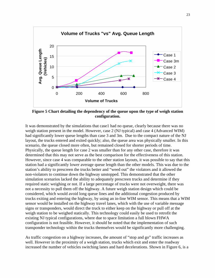
total volume of trucks for each scenario........................................................ 22 Figure 5 Chart detailing the dependency of the queue upon the type of weigh station

configuration.................................................................................................. 23 Figure 6 Chart detailing the cars which decelerated at a rate greater than 0.3g and trucks

greater than 0.2g for each weigh station configuration. ................................ 24 Figure 7 Vibratory compactor used to fabricate HMA brick samples.............................. 30 Figure 8 Diamond blade saw used to prepare HMA samples for epoxy evaluation tests. 31 Figure 9 Photograph showing epoxy infiltration into the grooves previously cut into the

HMA bricks. .................................................................................................. 32 Figure 10 Photograph of APA Test rutting results of PU-200.......................................... 34 Figure 11 Photograph of APA Test rutting results of E-Bond G-100. ............................. 35 Figure 12 Photograph of APA Test rutting results of ECM P5G. .................................... 36 Figure 13 Photograph of APA Test rutting results of AS 475.......................................... 37 Figure 14 Photograph of APA Test rutting results of E-Bond 1261................................. 38 Figure 15 Photograph of APA Test rutting results of Dural 306...................................... 39 Figure 16 Photograph of APA Test rutting results of Dural 340...................................... 40 Figure 17 Photograph of APA Test rutting results of Bondo 7084. ................................. 41 Figure 18 Photograph of APA Test rutting results of MM-80.......................................... 42 Figure 19 Photograph of vacuum container with vacuum pump and gage....................... 49 Figure 20 Addition of salt to form brine solution to ensure test would be performed under

worst case environmental effects................................................................... 50 Figure 21 Weighing of samples to determine saturated surface dry (SSD) weight.......... 50 Figure 22 Photograph of the three bricks, with three separate epoxy samples each

wrapped in saran wrap and sealed in plastic bags. ........................................ 51 Figure 23 Photograph of samples in freezer unit. ............................................................. 51 Figure 24 Free-Free Resonant Column tests results, frequency response of PU-200. ..... 57 Figure 25 Comparison of Elastic Modulus. ...................................................................... 59 Figure 26 Zone of Elastic Modulus close to that of HMA pavement in relation to the

remaining roadway epoxies ........................................................................... 60 Figure 27 Comparison of cumulative delamination of various epoxies to the ratio of

Coefficient of Thermal Expansion and ratiox10000 of Elastic Modulus at ~60oC of epoxies to HMA. ............................................................................ 61

Figure 28 APA testing of fourth prototype sensor, sensor assembly one (WIM1)........... 63 Figure 29 APA testing of fourth prototype sensor, sensor assembly three (WIM3). ....... 64 Figure 30 Comparison of sampling rate on the voltage output......................................... 66 Figure 31 Photograph of Asphalt Pavement Analyzer (APA) loaded with the samples and

connected to data collection computer. ......................................................... 69 Figure 32 Graphs of the raw results of the five (5) APA load wheel tests. ...................... 70 Figure 33 Photograph of rutting effects on the asphalt pavement (left) and concrete

pavement (right) samples............................................................................... 71

vii

Figure 34 Graph of combined rut data from APA test 0 thru 80,000 cycles. ................... 72 Figure 35 Rutting of asphalt sample after 100,000 cycles................................................ 72 Figure 36 Rutting of concrete sample after 100,000 cycles.............................................. 74 Figure 37 Shear stress crack observed in concrete sample after 100,000 cycles.............. 74 Figure 38 Voltage outputs of sensor embedded in asphalt pavement at 2000 cycles....... 75 Figure 39 Voltage outputs of sensor embedded in concrete pavement at 2000 cycles..... 75 Figure 40 Voltage outputs of sensor embedded in asphalt pavement at 20,000 cycles.... 76 Figure 41 Voltage outputs of sensor embedded in concrete pavement at 20,000 cycles.. 76 Figure 42 Voltage outputs of sensor embedded in asphalt pavement at 100,000 cycles.. 77 Figure 43 Voltage outputs of sensor embedded in concrete pavement at 100,000 cycles.77 Figure 44 Graphs of maximum positive and minimum negative voltage outputs of asphalt

and concrete samples over 100000 cycles. .................................................... 79 Figure 45 Graph of minimum negative voltage outputs of asphalt and concrete samples

over 100000 cycles. ....................................................................................... 79 Figure 46 Comparison of standard deviation of asphalt and concrete samples................ 80 Figure 47 Comparison of positive voltage output at 64oC (147oF) and 36oC (97oF). ...... 81 Figure 48 Comparison of negative voltage output at 64oC (147oF) and 36oC (97oF)....... 82 Figure 49 Route 287 weigh station static scale................................................................. 83 Figure 50 Route 287 Straight Line Diagram illustrating the weigh station section.......... 84 Figure 51 Combined northbound and southbound crash data for 2001 and 2002 along the

region of the weigh station and field implementation area............................ 85 Figure 52 Combined northbound and southbound crash data for 2001 and 2002 per mile

of roadway segment. ...................................................................................... 86 Figure 53 Photograph of Route 287 northbound at milepost 8.8, just prior to the weigh

station............................................................................................................. 86 Figure 54 Field observation of water ponding in the wheel paths.................................... 88 Figure 55 Final proposed location for the installation of the sensor assemblies. ............. 88 Figure 56 Photograph of ceramic-polymer composite sensor assembly and chairs laid-out

in the laboratory............................................................................................. 89 Figure 57 Photograph of the site layout for the installation of the sensors....................... 89 Figure 58 Photograph of wet saw cutting grooves for the sensors in the Route 287

inbound ramp. ................................................................................................ 90 Figure 59 Photograph showing the power washing and blowing of the groove to remove

debris and water. ............................................................................................ 91 Figure 60 Photograph of the groove with the wires and plastic conduit ready for epoxy

infiltration. ..................................................................................................... 91 Figure 61 Photograph of ceramic-polymer composite sensor assembly being placed in

groove at the Route 287 weigh station. ......................................................... 92 Figure 62 Photograph of PU-200 epoxy being placed in the bottom of the groove prior to

final placement of the sensor assembly. ........................................................ 93 Figure 63 Photograph of the completed WIM installation at the Route 287 weigh station.

....................................................................................................................... 93 Figure 64 Photograph of control/junction box linked to sensor wires and ready to be

buried. ............................................................................................................ 94 Figure 65 Ceramic-polymer composite sensor assembly initial field trial Rt. 287 results at

26.5 kph (16.5 mph)....................................................................................... 95

viii

Figure 66 Ceramic-polymer composite sensor assembly limited field trial limited field trial testing at 32kph (20 mph)....................................................................... 96

Figure 67 Ceramic-polymer composite sensor assembly field trial Rt. 287 results after winter season at 19 kph (12 mph).................................................................. 97


Figure 69 Ceramic-polymer composite sensor assembly field trial Rt. 287 results after winter season at 22.5 kph (14 mph)............................................................... 98


Figure 71 Ceramic-polymer composite sensor assembly results of tractor trailer loading, initial field trial Rt. 287 results at 72.5 kph (45 mph). ................................ 100

Figure 72 Ceramic-polymer composite sensor assembly field trial Rt. 287 results of tractor trailer loading, after winter season at 67.5 kph (42 mph). ............... 101

Figure 73 First axle loading results for the ceramic-polymer composite sensor assembly field trial Rt. 287 results of tractor trailer loading, after winter season at 67.5 kph (42 mph)................................................................................................ 101

Figure 74 Second axle loading results for the ceramic-polymer composite sensor assembly field trial Rt. 287 results of tractor trailer loading, after winter season at 67.5 kph (42 mph). ....................................................................... 102

Figure 75 Sample strain trace for various axle loading conditions.32 ............................. 103 Figure 76 Failure of sensor assemblies; outside of lane (left) and inside of lane (right).104 Figure 77 Close-up examination of failed outside of lane sensor assembly................... 105 Figure 78 Close-up examination of inside of lane sensor assembly............................... 106 Figure 79 Transverse stress distribution on roadway surface due to tire loading........... 107 Figure 80 Top-down fatigue cracking on Rt. 287........................................................... 107 Figure 81 Strain effects with respect to seasonal temperature variation versus distance

from center of wheel load.33 ........................................................................ 108 Figure 82 Recovered sensor assembly from Rt. 287 field installation. .......................... 109

1

ABSTRACT This research finished the development and implementation of a novel and durable, higher voltage, and lower temperature dependant weigh-in-motion (WIM) sensor that was begun under an earlier research project. These better sensors will require fewer lane closings and replacements than the existing sensors. They will also aid the Departments of Transportation to better identify those vehicles, which use the nations major highways, that do not comply with the current weight restrictions that are placed on larger vehicles. The primary focus of the research was to create a full scale WIM sensor that is less temperature dependent and more durable than traditional WIM sensors. Traditionally, the data collected from the sensor may be utilized in two ways. The first is by using static vehicle effects on the sensor, which corresponds to the weight of the vehicle, this data can be used for enforcement of the vehicle legal weight limits. The second is by using the dynamic loading of the sensor, which relates to the actual loading that the roadway is experiencing, this data will be useful to engineers who must design the roadway as well as plan for repair schedules. However, there is a growing trend to broaden the use of WIM data and use the data to its fullest extent. Instead of just using WIM data to screen commercial vehicles or for pavement design; there is a new recognition that good data can be useful for bridge structural analysis, safety analysis, traffic control and operations, freight management and operations, facility planning and programming, and standards and policy enforcement as per the recent report “Effective Use of Weigh-in-Motion Data, the Netherlands Case Study” FHWA October 2007. In lieu of this development, the need for better sensors to provide good data is more important today than ever before.

2

RESEARCH OBJECTIVES A fundamental question to be answered by this research is: Are piezoelectric ceramic materials, which generally have a stable response over a large temperature range, feasible as a weigh-in-motion (WIM) traffic data sensor in spite of their inherent brittleness? Currently, WIM systems use a piezoelectric polymer sensor that produces a voltage proportional to an applied pressure or load. Using this phenomenon, these systems are already being used to collect traffic data, including weigh-in-motion, measuring vehicle speeds, classifying vehicles by category and counting axles etc. The piezoelectric polymer sensors are usually in the form of a long tape or cable embedded within a long block of elastomeric material. These blocks are installed into grooves, which are cut into roads perpendicular to the traffic flow. The principal disadvantage of the present sensor technology is that the piezoelectric output is not uniform with temperature and time, thus leading to large uncertainty in the data collected. Piezoelectric ceramic materials have a much more stable response over a large temperature range. However, bulk ceramics are not used for traffic data sensors due to their inherent brittleness. Piezoelectric ceramic-polymer composites are made with an active piezoelectric ceramic embedded in a flexible non-active epoxy polymer. It was the intention of this work to utilize them for WIM applications by exploiting their flexibility and excellent piezoelectric properties similar to that observed in bulk ceramics. There are many factors that can affect the accuracy of a WIM system. The effect of the factors is variable, and complex interactions among the factors can occur. The net effect of all the factors at any given time is the main issue for the development of the piezoelectric ceramic-polymer composite WIM system. Each system has an associated level of accuracy – in terms of a tolerance and conformity. Therefore, it was the goal of this work to develop a sensor with a higher level of accuracy than can be attained by available WIM systems under actual field conditions.

3

INTRODUCTION TO WEIGH-IN-MOTION Introduction to Conventional Weighing Techniques There are many drawbacks to the present system of enforcement of weight restrictions for large vehicles on the major highways of the country. Historically, tractor-trailers and other large vehicles have traveled the highways virtually unchecked. Periodically, weigh stations on major highways are opened in order to enforce weight restrictions. However, when they are in operation many of the drivers for the larger trucking outfits purposely inform their colleagues via two-way radios. Once known the weigh station is open, the drivers direct other overweight trucks around these stations to avoid lost trucking time, possible hassles, and fines. In practice, it is widely believed that there is a significant discrepancy between heavy trucks which exceeded the legal weight limit and the ones that are caught and issued fines at the weigh stations. This discrepancy is believed to be as a result of overweight trucks bypassing the weigh station. Fines for overweight vehicles are generally a dollar a pound, and can easily total several thousand dollars per violation that the trucking companies must pay. Therefore, it is in the trucking company’s best interest to either keep their trucks under weight or somehow avoid getting weighed. This bypassing practice is unethical and not officially endorsed by the trucking companies, but nonetheless it occurs. Additionally, in States where the weigh stations do not operate continuously 24 hrs/7 days a week, many overweight vehicles are not detected simply because the station is closed. Also, even when the stations are open they frequently close due to lengthy queue waits; and once again overweight vehicles are not identified because the station is temporary closed due to queue backup.

Once open, the operators of the weigh stations usually turn on a sign instructing drivers to pull off the highway and enter the weigh area. It usually takes anywhere from 30 seconds to 5 minutes to weigh each truck, check vehicle loads, and perform a safety check.1 Once about 15 trucks have lined up in the station, it has to be closed to avoid traffic back-ups on the highway. Only after these trucks have cleared the weigh station, the operators reopen the station and direct trucks to pull off the highway once again. During one day of operation a large number of trucks are weighed, however many trucks simply ‘get lucky’ and are able to bypass the station while the operators are trying to handle the trucks already in the queue. In general, there are two types of weigh stations: ones that are in continuous operation and ones that are open at random to keep the trucking companies constantly on their feet. Additionally, the non-continuous ones are not even open for 40 hours a week, so they cannot offer proper and continuous monitoring of weight restrictions. Thus, many overweight trucks pass through the highway system everyday, a safety threat to the infrastructure and other vehicles.

There are other disadvantages to this system of collecting data. It is known that there is a lot of wear and damage to the asphalt pavement roadway caused by the stopping and starting of vehicles. The horizontal friction forces created by braking and acceleration of the trucks at the weigh stations can cause excessive rutting and shoving to occur in the vicinity of the station. The stopping of heavy tractor-trailers subjects the road to negative conditions that over time can accelerate the deterioration of the highway.2 The impending wait in the queue also costs businesses time and money in delayed shipments.

4

Weigh-In-Motion Definition The process by which the dynamic tire forces of a moving vehicle are measured and used as the basis for estimating the corresponding static weight of the vehicle is called weigh-in-motion (WIM).

A WIM system consists of a set of sensors and data collection/analysis equipment. The sensors detect the presence of a moving vehicle and the related dynamic tire effects with respect to time. The data is collected and processed to estimate a vehicle weight, speed, axle spacing, and vehicle class according to the number of axles and the axle spacing.

Weigh-in-Motion Systems In order to overcome the problems related with traditional systems, many of the state Departments of Transportation (DOT) are using weigh-in-motion (WIM) systems to compute the weight of vehicle axles. WIM systems estimate a moving vehicle’s gross weight that is carried by each wheel, axle, and/or axle group, by measurement and analysis of dynamic forces applied by its tires to a measuring device.1 At the time this research began, most of these systems used piezoelectric polyvinyldine fluoride (PVDF) piezoelectric materials, for example, the extremely popular Brass Linguini (BL) sensor is a P(VDF-TrFE)3, polymer sensors for the collection of traffic data. The polymer in either tape or cable format is embedded within a long block of elastomeric material that is then installed in a narrow groove on the highway. The sensor receives a portion of the full load of the passing vehicle’s weight and gives a voltage output that is translated into the weight of the truck. The principal advantage offered by WIM sensors include the ability to continuously measure weights of the trucks traveling on the highway at various speeds, without diverting or stopping them. It can also keep a count of the number of vehicles, measure their speeds, classify them according to weight category, and detect the number of axles. Apart from the above applications, this type of sensors could also be used for parking area controls, tollbooth systems, scale operations, and freight yards.4 Despite all of the highlighted advantages, the present WIM technologies using PVDF polymer sensors have two main drawbacks. The first is the variability in the voltage output that is mainly attributed to temperature fluctuations. In order to incorporate voltage variations with respect to temperature changes from day to night and different seasons, the piezoelectric sensors are calibrated and have a built in temperature correction algorithm. However, many times this temperature correction methodology cannot correct for the hysteresis that the PVDF WIM sensors experience, and without constant recalibration the WIMs show readings that are simply put unreasonable.5 The other major drawback is that the polymer sensors are more prone to physical damage under heavy loads leading to sensor failure. Based upon many recent WIM installations, the sensors do not seem to last their expected service life of about two years.4

A recent NCHRP Study Synthesis 386, published in 2008, conducted a nationwide survey of all 50 States, DC, and Puerto Rico. One of the survey questions was “In your opinion, what are the most urgent WIM technical needs at present and what studies need to be conducted to address

5

them?” A summary of relevant comments from the respondents is provided in Table 1. In general, respondents wanted more accurate, more durable, and less temperature dependant sensors as well as better epoxies/grouts to ensure installations last longer.

Table 1 Summary table of WIM technical needs as PER NCHRP Survey Synthesis 386.6 In your opinion, what are the most urgent WIM technical needs at present and what studies need to be conducted to address them? MT-Traffic: Better, more reliable sensors. Better epoxy. Modernize the electronics to reduce power consumption and footprint. Improve communication techniques for retrieving data. Temperature of road (sensors) factored into auto calibration routines for systems using sensors that are temperature sensitive. Better software for both office and field operations. Software needs to be modernized to work with today's operating systems, and it needs to be more user friendly, especially for those users who are not technically inclined. Sensor and epoxy studies should be a joint venture between states and vendors. Software and communications upgrades should be performed by the vendors in response to their customers' needs. Factoring in temperature as part of maintaining calibration on temperature sensitive sensors could also be a joint venture with states. Joint studies (vendors and states) have one major drawback--time. Since it appears that most states are understaffed in their traffic data collection areas, participation from a state standpoint would be nearly impossible to do. Once again, if FHWA truly believes that this data is important, then they need to work with state legislatures to make sure that adequate staff is obtained, not only to collect and process data, but to aid in the advancement of data collection tools and methods. NM-Traffic: making the BL piezos last longer regardless of what kind of traffic WA-Traffic: As you all know, BL piezos are temperature and speed sensitive. I've talked to IRD to expand their temperature and speed bins, but they said there was limitation to the DOS operating system's memory. If all of us can pitch in some money to pay for IRD to develop their WIM software in Windows that would be a plus. NJ: Develop more accurate sensors. VA-Traffic: Smoother, more wear resistant pavement. Sensors with reduced sensitivity to rutting. Lower cost sensors. SC: Sensor accuracy. Temperature and so called "auto cal" corrections to WIM data. CO-Traffic: Better grouts for piezos and for CDOT better accuracy out of our roadway sensors. WY-Traffic: From a Type II WIM perspective sensors are still the weak link. I feel fiber optics may hold promise and warrant increased study. GA: Technological improvement NH: Sensors and installation methods that last. Please provide any additional comments you may want to share about high speed WIM calibration. NM-Traffic: manufacturing better piezo's to last at least 5 years NJ: Percentage of errors changes with temperature change. Properly calibrated system verified in the morning will have a significant error in the afternoon? Does test truck calibration really makes that much difference?

6

Introduction to Piezoelectricity Piezoelectric; the word is derived from the Greek “Piezin“, which means to squeeze or press. Thus piezoelectricity is really “pressure electricity.” Piezoelectric implies that the material has a crystalline structure, quartz for example commonly found in watches exhibits piezoelectric properties. Ceramic materials such as PZT (Lead Zirconate Titanate) are crystalline, but the crystals are very tiny. PZT is a piezoelectric material through a combination of chemical effects, physical effects, and geometry. Unlike quartz, PZT starts with powdered crystals which get melted together and solidify into a block so it is not just a single crystal, but numerous small ones. Once the block is formed it is still not a piezoelectric material, its all scrambled, think of it in terms of magnetism with pluses and minuses more or less it is an equal balance but by aligning the charges a block of ceramic (containing all these tiny crystals) can be “poled” Figure 1a. Poling is done with heat, pressure, and exposing the material to a strong voltage/electrostatic field Figure 1b. When the material cools it retains this internal electrical alignment, as shown in Figure 1c. However, exceeding the materials’ remnant polarization properties thermal, mechanical, or electrical will cause its polarization to degrade.7

7

Figure 1 Diagram detailing the poling process and remnant polarization.

Now, the material has a distinct electrical pattern, as the material is squeezed the small internal charges will seek out their opposites and flow together. During the poling process the material permanently elongates, this material can be thought of as stretched. Therefore, by creating an imbalance in the ceramic itself like a stretched rubber band the sample now has the electrical equivalent of basic physics’ potential energy, but in this case static electricity. PZT crystallites are a symmetric cubic but when a voltage is applied the structure becomes tetragonal, or vice versa when a load is applied. Therefore, the Zirconate Titanate is pulled toward the positive potential. With the lead crystal around it, the structure will change in dimensions to accommodate the new position of the Zirconate Titanate. As a result, there is a distortion which causes growth and an alignment of field, see Figure 2. As all the crystals are doing this at the same time and have the same electric dipole domain alignment; the crystals thereby generate a voltage, the cumulative of which can be quite large.

a. Unpoled electric dipole domains in random orientation

b. Polarization (heat and electric field) causes the

electric dipole domains to align

c. Remnant polarization, electric dipole domains

remain roughly aligned after cooling and removal of field

8

Figure 2 Diagram detailing the piezoelectric effect of PZT.8

Movement of Ti, Zr towards positive potential

9

Principle of Piezoelectricity The output variations and the premature failures of the WIM sensors are mainly related to the kind of piezoelectric sensor material used in the assembly. Therefore, it was important to understand the phenomena of piezoelectricity and know about the different types of piezoelectric materials available for use as sensors. This could help in avoiding the problems faced with the present technology. The piezoelectric effect occurs in a number of single crystals, polymers, and ceramics. The direct piezoelectric effect relates a change in the polarization (charge) to an applied stress, whereas the converse effect relates a dimensional change to an applied electric field. Piezoelectric sensors, which convert mechanical energy to electrical energy, have found applications as sensors in many areas including car tilt control, hydrophones, and lighters to name a few.9 For typical WIM systems, a piezoelectric polymer sensor assembly is embedded under the road, and the weight of the wheels of a vehicle passing over it leads to the creation of electrical charges on the opposite faces of the sensor. The total voltage generated due to the application of pressure depends on the properties of the piezoelectric material used for the sensor. They are related by,

V = (d33 • σ3 • A ) / C

where V is the voltage generated, A is the sensor surface area, σ3 is the applied stress, and C is the capacitance of the sensor. The amount of charge generated would depend on the piezoelectric charge coefficient ‘d’ of the material. For a sensor poled in the thickness direction and for pressure applied in the same direction, the piezoelectric charge coefficient would be equal to the d33 coefficient.

In order to obtain a high voltage output, it is necessary to have a large charge output, for example by using a material with a high d33 coefficient. Also, it is important to note that the total capacitance should also be as low as possible, the higher the capacitance the more it will degrade the output voltage. Even though the capacitance of the cables are typically very low (100 pF/m), the cables should be kept as short as possible, to help maximize the net voltage output. However, in actual practice the cables from the sensors have to be routed from the roadway to the measurement electronics that are usually at the edge of the highway. The voltage drop due to cable length increases has to be considered if extended lengths are necessary, otherwise there is not much that can be done to minimize capacitance effects further.10

Weigh-In-Motion and Dynamic Forces Weigh-in-motion systems do not actually weigh the axles crossing the sensors, instead sensors measure the dynamic force present when each axle crosses the sensing unit. The entire process is a result of several different phenomena acting simultaneously. The movement of the suspension, body and the load, and an unbalance in these various components, will create vertical and lateral oscillation of the vehicle. Also, speed and ride quality of the surface and pavement conditions produce vibrations in the suspension and the vehicle body. These factors can increase errors in the sensing units and data analysis. These conditions result in the dynamic forces being observed

10

by the weigh sensors, which therefore result in a weight either greater or less than the true static weight. Such variations can be as much as plus or minus 30-40% of the static weight.

Accuracy of Weigh-In-Motion Systems Accuracy is the quality of conformity of a measured value to an accepted standard value. The overall accuracy of a WIM system is a function of the actual difference in the dynamic tire force of the moving vehicle and the corresponding constant tire force of the static vehicle. There are many factors that affect the accuracy of the WIM system, the type of sensor is only part of the equation as the sensor experiences many variables in a real world environment. This is affected by factors such as:

• Gross vehicle weight. • Distribution of Gross vehicle weight. • Suspension. • Tires, aerodynamic alignment of roadway and road surface. • Accuracy of the dynamic tire force measurement. • Force sensor location. • Sensitivity to direction of force application. • Tire inflation pressure effects. • Contact area effects. • Mass stiffness and damping of sensor. • Durability and stability. • Calibration and measurement. • Adequacy of the estimation procedure. • Analog to digital conversion. • Filtering. • Averaging. • Detection of peak values in a dynamic force signal. • Integration of instantaneous measurements. • Accuracy of the weight measurements for the static vehicle. • Type of weighing device (vehicle scale, axle-load scale, etc.). • Inertial forces. • Speed of the vehicle. • Environmental conditions, thermal properties of the materials. • Lane drift of the vehicles.

Past Weigh-In-Motion Research Weigh-in-motion (WIM) technology provides information on the characteristics of traffic loads, speeds, and vehicle classification for the purposes of roadway design as well as for weight regulation and enforcement. Currently, there are many accepted systems in use today across North America and around the world. WIM systems collect data under a variety of dynamic and environmental conditions. The WIM systems measure several data elements then process the

11

data to report a wide range of axle loads. However, due to the harsh and dynamic nature of the environment as well as shifting calibration this combination of factors resulted in WIM outputs being frequently rejected and considered unreasonable.5 There is much debate as to what data is real and what data is a misread. Therefore, there is extensive nationwide and international research for the evaluation and calibration of alternative WIM system configurations. Indeed this is a global problem, and in one such study performed by The University of Manitoba, Department of Civil and Geological Engineering11, a survey was conducted to simultaneously collect data from a major WIM site that participates in the Long Term Pavement Performance (LTPP) program and from a static permanent truck weigh station. Pairs of matching records were examined to assess the quality of WIM data and to develop relationships among the axle loads, axle-spacing, gross vehicle weight (GVW), and vehicle lengths as well as to evaluate WIM’s abilities to classify vehicles. The study documented the performance of the WIM systems installed at six places in Manitoba, in terms of reasonableness of WIM data, physical conditions of WIM sites and calibration techniques. The results of the study are:11

• None of the WIM systems functioned year-round, • The features of a site significantly affect the performance of a WIM system. The ideal

conditions are achieved when force is applied to a smooth and level road surface by perfectly round and dynamically balanced rolling wheels.

• Four group factors as indicated by Lee (1988) , may cause the difference between WIM and static measurements:12

o Dynamic factors (e.g., vehicle speed, vehicle suspension system, and wheel path profile of pavement);

o Equipment (e.g., WIM sensor used); o Signal interpretation; o Static reference (e.g., static axle-group load and static GVW).

• WIM errors are comprised of systematic errors and random errors. The purpose of WIM system calibration is to reduce systematic errors. The “out-of-calibration” problem is experienced by many WIM systems and it was found that it generally starts 3 months after the system calibration. The outcome of the drift is different from site to site.

• The paper concluded that 90% of GVWs were underestimated by the WIM system during the hours of the survey. Under the acceptable tolerance for the WIM weights specified by American Standard for Testing and Measures (ASTM), the WIM system was not capable of meeting the specified accuracy limits.

WIM Installation and Maintenance Costs Breakdown In 2004, the National Cooperative Highway Research Program (NCHRP) conducted a study on equipment for collecting traffic data. Below is Table 2, which shows the various WIM equipment options and their associated life cycle costs. These costs that were considered ignored the pavement rehabilitation aspect. The paving cost could be the most substantial component of the all the various costs. If concrete is selected, the most significant costs are upfront during construction; as opposed to asphalt pavement in which the costs will be dispersed over cyclic rehabilitation periods. The cost of the WIM sensors are relatively inexpensive, it is actually the cost of installation that represents the majority of the cost. This merely proves that a more

12

durable WIM sensor that might cost a little more than the standard WIM would be highly desirable considering the other expenses and the other WIM technology costs.

Table 2 NCHRP Table estimating WIM equipment initial and recurring costs.13

Permanent WIM Operations WIM data collection using permanently installed weight sensors installed in the roadway surface is now quite common in the U.S. By installing the sensors in the roadway, this eliminates or significantly reduces the bump that vehicles experience when crossing surface-mounted sensors. By engineering the sensor such that it is flush to the pavement surface, it therefore minimizes the sensor error caused by the extra vertical motion, which in general should result in improved system accuracy.13

13

Another major advantage of installing the sensors flush to the pavement is that it decreases the impact loads on the sensors themselves. This basically reduces the wear not only on the sensor, but also on the surrounding pavement. There are several WIM technologies that can be used for permanent, continuous weight data collection, these are:13

• Capacitance mats, • Piezoelectric sensors; Ceramic, Polymer, and Quartz • Bending plates, • Load cells, • Bridge and culvert WIM systems, and • Other WIM technologies (fiber-optic, subsurface strain gauge, multi-sensor).

For the purposes of this effort, only Piezoelectric sensors; Ceramic, Polymer, and Quartz have any direct bearing on the research work performed. Therefore, a brief description of each technology is included in the following section. Site installations for either of the three are basically the same, and can consist of two piezoelectric sensors, two sensors plus an inductance loop (as it appears in Figure 3), or one piezoelectric sensor and two inductance loops.

Piez

o1

Piez

o2

Loop1 Loop2

Cabinet & Base

Junction Box

Shoulder

Median

Figure 3 Example of a typical piezoelectric WIM system layout

14

The installations using two piezoelectric sensors tend to provide better estimates of static axle weights because each sensor provides an independent measure of axle weight, which can be compared to identify any discrepancy due to vertical motion of the vehicle. Combining the two independent weight estimates generally improves the accuracy and reliability of the estimates of the static weight calculation.13

Piezoceramic Sensors Piezoceramic sensors use ceramic material which is compressed between an outer sheath of copper. Typical piezoceramic sensors, like the Thermocoax/Vibrocoax sensor, closely resemble the size, shape, and internal configuration of conventional coaxial cable.13 These types of sensors have lost considerable favor in recent years due to durability problems, and have largely been replaced in the market by piezopolymer sensors.

Piezopolymer Sensors Piezoelectric polymers will be discussed at length later in this study. However, the most popular commercially available sensor of this type is the Brass Linguini (BL) sensor. The flexible nature of the polymer allows for a more liberal approach in handling when conducting the installation. In addition, it is relatively low cost to purchase the materials, therefore making the installation process the cost restrictive factor and not the sensor. This sensor has similar characteristics as other piezoelectric sensors and has essentially the same benefits and drawbacks but at a relatively low cost. However, the BL sensor is also temperature sensitive, and the piezoelectric effect it generates is dynamic.13

Piezoquartz Sensors The piezoquartz sensor differs from the other piezoelectric sensors both in the piezoelectric material used and in the design of the sensor itself. In general, the piezoquartz sensor is more expensive per sensor than the other piezoelectric style sensors. The piezoquartz sensor also has the distinct advantage of being insensitive to changes in temperature. Therefore, it is generally more accurate than other typical piezoelectric sensors. However, because the sensor still relies on structural support from the pavement, the variability of the sensor due to the underlying pavement is still an inherent issue. The sensor will still show some changes in response to a given axle load simply as a result of the change in pavement flexural stiffness due to temperature changes.13

15

DEVELOPMENT AND EVALUATION OF THE SENSOR

Conclusions from Previous Research

Based on the results of the initial sensor fabrication effort as reported in the Implementation of Advanced Fiber Optic and Piezoelectric Sensor – Fabrication and Laboratory Testing of Piezoelectric Ceramic-Polymer Composite Sensors for Weigh-in-Motion Systems” FHWA-NJ-1999-029 also written by the author of this report, the following can be concluded:

• It was shown that for PVDF polymer sensors versus the ceramic-polymer

composite sensor, under the same loading conditions, that the average loading output of the composite sensor is about three times that of the PVDF sensor.

• The ceramic-polymer composite sensor has superior electrical properties than that of the PVDF, including a higher d33 and thickness-coupling coefficient. The signal to noise ratio is also much better for a ceramic-polymer composite sensor and hence will detect much lower load differences with a greater accuracy.

• For a piezoelectric material, when the temperature approaches the Curie temperature (Tc) where the aligned electric dipoles are easier to rotate under heaving loading the material will depole; i.e. hence a degradation in the sensor performance. The PVDF has a Tc of only 100oC (212oF) it could easily start losing part of its piezoelectric properties at high loads at temperatures as low as 55-65oC (131-149oF). To avoid thermal depolarization a “safe operating temperature would normally be about half way between 0oC and the Curie point”14 For the PVDF materials this implies that that use above 60oC (140oF) is not recommended. This limit 60oC (140oF) is dangerously close to the upper thermal limit of 64oC (147oF) in summer within a 98% reliability15 as per FHWA that HMA experiences in New Jersey. However, the ceramic-polymer composite sensor is more rugged with a much higher Tc of ~190oC (374oF).

• The laboratory results from the initial prototype, voltage output with respect to loading and temperature proved to reliably yield the same results or at least the same trends.

Utility of an Improved WIM – Traffic Simulation Modeling It was the overall goal of this research effort to develop a more accurate and durable WIM sensor. Increased durability and longevity are obviously beneficial; however, what affects will a more accurate sensor have on operations? Therefore, the focus of this section was to develop weigh station models that accurately predicted the effects of various weigh station configurations using various levels of technology (and accuracy) in their design. Thus validating the benefits and need for the development of the ceramic-polymer composite weigh-in-motion system. Three (3) traffic volumes were used to test five (5) different weigh station conditions. The three (3) traffic volumes were the Annual Average Daily Traffic (AADT), Annual (Worst Case) Peak

16

1hr Traffic, and Annual Maximum Daily Traffic (BEST DATA). The five (5) weigh station configurations were the Existing Conditions Closed Station (No WIM and Closed Scale), Modified FHWA Configuration (No WIM and Scale), Existing Conditions Open Station NJ Typical Configuration (No WIM and Scale), FHWA Configuration (WIM and Scale), and the Advanced FHWA Configuration (Advanced WIM and Scale). The models were evaluated using the following criteria: trucks should experience a decrease in queue time, automobiles should experience a more continuous flow on the highway, nearly 100% of all overweight violators should be issued violations, almost all the vehicles should be weight evaluated without actually stopping all the vehicles for static weighing, and the number of vehicles making a hard deceleration will be the lowest. If a more accurate WIM sensor could augment a static scale and improve these criteria then there is most definitely a need and therefore the ceramic-polymer composite weigh-in-motion system development was warranted. Weigh Station Drawbacks and Advantages There are many drawbacks to the present system of weigh stations and enforcement of weight. The impending wait in the conventional weighing queue costs businesses considerable losses in delayed shipments and wasted fuel. The maneuvering of trucks through traffic to stop at a weigh station causes additional vehicle congestion on the roadway. The weigh station queue lines can cause tractor trailers to back-up into the highway, thus causing vehicle intensification once again resulting in roadway congestion. In general, in addition to enforcement the use of WIMs can be used to obtain better data on highway usage for design purposes. The WIM systems can give designers actual axle weights of every vehicle on the roadway. WIMs can help generate better repair, maintenance, rehabilitation, and capital improvement scheduling. Since roadways and bridges are designed to carry a certain number of equivalent single axle weights during their design lifetime, a more accurate repair schedule can be created/modified with WIM data that is collected. In addition to all these benefits, WIMs can in theory be used to pre-screen trucks prior to arriving at static scales and thereby can reduce the number of vehicles that are required to actually exit the roadway to the scale station. Consequently, this would also benefit roadway maintenance, by decreasing horizontal friction forces created by braking and acceleration of the trucks at the weigh stations. In addition by using WIMs to prescreen trucks, they may also help to prevent excessive rutting and shoving in the vicinity of the station by reducing the number of trucks braking. Justification for Model Development The main goal of this section was to determine if the development of a new sensor was warranted by evaluating the effects of a WIM on weigh station functionality using simulations to predict performance. Weigh stations and truck weighing protect highways, bridges, and the public investment by prolonging the life of infrastructure. However, the introduction of a new sensor does not necessarily guarantee a significant increase in transportation efficiency; such as by minimizing unnecessary stops and delays, producing cost savings in faster deliveries and

17

reduced fuel emissions, or generating regular compliance. Therefore the impact of a more accurate sensor needs to be evaluated. According to the Brass Linguini (BL) (a commonly used WIM throughout the U.S.) manufacturer, currently their Class II WIM sensors have a uniformity of +/- 20% and are only typically used for classification purposes. Also, once again according to the manufacturer, their Class I sensors have a uniformity of +/- 7% which are typically used for WIM applications.3 However, over time the uniformity of the sensors typically degrades, therefore for the purposes of this model a 10% accuracy was assumed for existing technologies. This was in keeping with ASTM standards E1318, where a Type I WIM sensor must have a functional performance accuracy of 10% for the gross vehicle weight.16 Please note that Class I and Class II as described by the BL manufacturer are different than the ASTM Type I and Type II classifications. As a frame of reference, the required accuracies as specified by ASTM are listed in Table 3. Type I and Type II are very similar, other than the accuracy level and the fact that Type I sensors must be designed for installation into up to four lanes; they must be able to accommodate speeds from 16 kph (10 mph) to 113 kph (70 mph) and acquire the data listed in Table 3. However, in general Type III WIM systems are to be designed for one or two lanes operating at speeds from 24 kph (15 mph) to 80 kph (50 mph) and are to be used for weight limit or load limit violations. The big difference between Types I and II versus Type III is the “violation aspect” and therefore it requires a higher degree of accuracy. Type IV is very similar to Type II, but Type IV is used for low speeds from 0 kph (0 mph) to 16 kph (10 mph) and requires the highest accuracy.16

Table 3 Summary table of WIM system requirements as per ASTM E1318.16

Value >= kg (lb) +/- kg (lb)

Wheel Load 25% 20% 2300 (5000) 100 (250)

Axle Load 20% 30% 15% 5400 (12000 200 (500)

Axle Group 15% 20% 10% 11300 (25000) 500 (1200)

Gross Vehicle Weight 10% 15% 6% 27200 (60000) 1100 (2500)

Speed

Axel Spacing

Tolerance for 95% Probability of Conformity (all percentages shown +/-)Function Type IV

+/- 2 kph (1 mph)

+/- 150 mm (0.5 ft)

Type I Type II Type III

It was estimated that based on the ceramic material being less temperature dependant, that a uniformity of 5% or better could be expected from a ceramic-polymer composite sensor. It is this basic uniformity consideration that will be evaluated in this model to determine what if any effect the increase in uniformity will have on static scale operations.

18

Modeling of Route 287 Weigh-In-Motion (WIM) Installation Prior to evaluation of the utility of a ceramic-polymer composite sensor, a model was developed to evaluate if the ceramic-polymer composite sensor was feasible as a traffic sensor. Laboratory testing needs to be conducted prior to making this final determination. However, before the laboratory testing was conducted, a model needed to be developed to validate the need for the development of the sensor. Based on past publications and the basic principals of piezoelectricity and ceramics, certain assumptions were made regarding the performance of the proposed sensor. A test site was not available for a field installation at the time the model was generated. Therefore, based on the high level of traffic and the availability of traffic data, real I-195 Eastbound highway data from the Special Pavement Study (SPS) data from the Long Term Pavement Performance (LTPP) group of the Federal Highway Administration (FHWA) was used. The SPS data helped generate the vehicle distributions. Thus, the class distribution was generated from this data. The traffic count records of the New Jersey Department of Transportation (NJDOT) were used to generate flows for each lane. These flows were then used as an average to estimate time between vehicles in the model. The Five (5) Weigh Station Configurations

1. Existing Conditions Closed Station (No WIM and Closed Scale) Currently, the roadway has two lanes in the east bound direction in the Freehold area. This model established a baseline in order to compare the other models. The scenario where the scale is closed and no WIM exists is the same as if the station was nonexistent. 3m. Mod. FHWA Configuration (No WIM and Open Scale) This model used the typical layout specified by the FHWA for weigh stations, with one exception, the model lacks any WIM scale. This model established a minimum performance of the elaborate FHWA station design. 2. Existing Conditions Open Station NJ Typical Configuration (No WIM and Open Scale) This model was based on the standard New Jersey weigh station layout used throughout the state (except near the Delaware Memorial Bridge where they use the FHWA configuration). The ramps are fairly short and the scale is very close to the roadway, approximately 6 m (20 ft). The station is comparatively small and even though a WIM can be installed, there is not enough space for a bypass lane, making the WIM rather ineffectual. However, since this is the most common design used in New Jersey, the results should provide some insight. 3. FHWA Configuration (WIM and Open Scale) This model used the typical layout specified by the FHWA for weigh stations. In general, this weigh station layout is rather large and is used in areas where there is still plenty of room for development around the highway. This model was based on the elaborate FHWA station design similar to that currently in place near the Delaware Memorial Bridge. The WIM system modeled was a traditional WIM with an expected error of 10%, thus building on the performance baseline established in model 3m.

19

4. Advanced FHWA Configuration ( Advanced WIM and Open Scale) This model also used the typical layout specified by FHWA for weigh stations. This model used the same methodology as Case 3, but used a new WIM sensor with better accuracy. Historically, WIM standard deviations range from 3-8%. Therefore, for the purposes of this model, the accuracy of the new advanced WIM was set at 5%. It should be noted that just because the accuracy of the WIM increased, this does not automatically guarantee that this model would outperform the others. The model has many complex interactions with numerous vehicles entering and exiting the roadway and a prediction could not be made prior to running the simulations. This model in comparison with the performance of the other four (4) models would determine if the potential sensor warranted development. The Three (3) Evaluated Traffic Flows A. Annual Average Daily Traffic (AADT) The Annual Average Daily Traffic (AADT) is the average traffic volume that the highway experiences in a year at a given location. This annual average was converted to an hourly volume and used in the model. This produced a fairly low estimate of vehicular traffic 24 hr/365 day average. In general, the AADT provided a good baseline, but is rather poor for any true design or analysis. B. Annual (Worst Case) Peak 1hr Traffic This is the absolute worst case scenario. The data for each hour of flow was collected for an entire year, and the single highest traffic volume was determined. This worst case will produce extreme results. For an entire year the road will be a fairly low estimate of vehicular traffic 24 hr/365 day average. Once again, this flow provided a good baseline, but would be considered poor for any design or analysis. C. Annual Maximum Daily Traffic (BEST DATA) This is the average annual maximum daily traffic volume that the highway experiences in a year. This means that the roadway experiences this maximum on a daily basis during its peak hourly flow. This is an accurate estimate of what the roadway experiences on a daily basis during peak flows. This flow was considered better than the others from a design and analysis perspective than the other flows. Layout and WIM Details A weigh-in-motion scale can pre-screen the trucks in the simulation. The WIM scale may be on the mainline or on a lower speed lane within the weigh station. Trucks measuring less than a specified threshold are directed to return to the highway. Trucks measuring greater than the specified threshold are directed to proceed to the static scale, queuing, if necessary. This study modeled various configurations some using WIMs and static scales; others using only static scales. In general, WIM scales are not as accurate as traditional static scales at measuring gross vehicle weight. The standard deviation of traditional WIM sensors are reported to range anywhere from 3% to 8% of the true truck weight, but in actual practice might be closer to 10%. Thus, the number of vehicles that are overweight but fall into the error range of the WIM is directly related to the WIM error. Thresholds on what the WIM identifies as under the legal limit must be lowered in order to ensure identification of true overweight vehicles. Conversely based on the

20

error, numerous underweight trucks near the legal limit will also be falsely identified and weighed on the static scale.17 Westa Model Westa (short for Weigh Station) is a microsimulation model built by Mitretek Systems. It is written in the C++ computer language and runs on any IBM-compatible personal computer.17 The Westa model was used to produce the results documented in this section. Summary and Analysis of Traffic Simulation Table 4 provides a summary of the major points of comparison for each model. Notice that each model was run three individual times; this was done to use various seed values to prevent the simulation from being one dimensional. This allowed an average of three runs to be taken and used in the verification of the results. A detailed analysis of these values are included in the following sections.

21

Table 4 Table summarizing major points of each model.

22

As shown in Figure 4 below, at low volumes any one of the models could identify all the overweight trucks. However, as the volumes increased only the weigh station models which used WIM sensors avoided bypassing (allowing trucks to skip being weighed) overweight vehicles. Such models as the conventional NJ standard weigh station configuration barely identified 40% of the violators. The FHWA standard configuration identified 70-80% of all violators. Using the advanced WIM sensor this model was projected to catch upward of 95% of all the violators.

M o d e l W o r k i n g V e r i f i c a t i o nV o l u m e v s V i o l a t i o n s

0 . 01 0 . 02 0 . 03 0 . 04 0 . 05 0 . 06 0 . 07 0 . 08 0 . 09 0 . 0

1 0 0 . 0

~ 1 8 0 ~ 5 9 0 ~ 6 5 0

T r u c k V o l u m e s

OVW

T Tr

ucks

Issu

ed

Viol

atio

n (%

) C a s e 1C a s e 3 mC a s e 2C a s e 3C a s e 4

Figure 4 Chart showing the percentage of overweight trucks issued violations versus the

total volume of trucks for each scenario. As the volume of trucks on a roadway increases it is the natural tendency of a queue to increase in length. However, the amount the queue increases is dependant upon the type of weigh station present, as shown in Figure 5.

23

Volume of Trucks "vs" Avg. Queue Length

0

5

10

15

20

0 200 400 600 800

Volume of Trucks

Avg

. Que

ue L

engt

h (V

ehic

les)

Case 1Case 3mCase 2Case 3Case 4

Figure 5 Chart detailing the dependency of the queue upon the type of weigh station

configuration. It was demonstrated by the simulations that case1 had no queue, clearly because there was no weigh station present in the model. However, case 2 (NJ typical) and case 4 (Advanced WIM) had significantly lower queue lengths than case 3 and 3m. Due to the compact nature of the NJ layout, the trucks entered and exited quickly; also, the queue area was physically smaller. In this scenario, the queue closed more often, but remained closed for shorter periods of time. Physically, the queue length for case 2 was smaller than for any other case, therefore it was determined that this may not serve as the best comparison for the effectiveness of this station. However, since case 4 was comparable to the other station layouts, it was possible to say that this station had a significantly lower average queue length than the other models. This was due to the station’s ability to prescreen the trucks better and “weed out” the violators and it allowed the non-violators to continue down the highway unstopped. This demonstrated that the other simulation scenarios lacked the ability to adequately prescreen trucks and determine if they required static weighing or not. If a large percentage of trucks were not overweight, there was not a necessity to pull them off the highway. A future weigh station design which could be considered, which would avoid long queue lines and the additional congestion produced by trucks exiting and entering the highway, by using an in-line WIM sensor. This means that a WIM sensor would be installed on the highway travel lanes, which with the use of variable message signs or transponders, would direct the truck to either keep on the highway or pull off at the weigh station to be weighed statically. This technology could easily be used to retrofit the existing NJ typical configurations, where due to space limitation a full blown FHWA configuration is not feasible. However, it should be noted that the implementation of such transponder technology within the trucks themselves would be significantly more challenging. As traffic congestion on a highway increases, the amount of “stop and go” traffic increases as well. However in the proximity of a weigh station, trucks which exit and enter the roadway increased the number of vehicles switching lanes and hard decelerations. Shown in Figure 6, is a

24

representation of all cars which decelerated at a rate greater than 0.3g and trucks greater than 0.2g during the simulation. Thus, the hard decelerations or hard braking was a very important factor to consider when evaluating a weigh stations’ feasibility. In the simulations, it was found that even without a weigh station there were a number of vehicles hard decelerating at higher traffic volumes. For example, at a volume of 4600 vehicles per 2 hour period, the percentage of vehicles hard braking was approximately 25%.

Total Volume "vs" Hard Decelerating Vehicles

0

1000

2000

3000

4000

5000

0 1000 2000 3000 4000

Hard Deceleration (vehicles)

Volu

me

of V

ehic

les

Case 1Case 3mCase 2Case 3Case 4

Figure 6 Chart detailing the cars which decelerated at a rate greater than 0.3g and trucks

greater than 0.2g for each weigh station configuration. The WIM simulations at higher volumes produced more hard decelerations than other configurations. This was most probably due to the increased complexity of lane changes and speed variations associated with the nearly all the trucks affecting the traffic flow. Since the WIM is more efficient, almost 100% of all trucks must exit the highway, (i.e. none are allowed to bypass the scale due to queue length backups) even if they are only going to pass over the WIM. Whereas before the queue would fill rather quickly and a large amount of trucks would bypass, therefore not having to slow down or exit the highway. With more vehicles changing lanes and more trucks exiting/entering the highway, the majority of the vehicles will be traveling at a non-consistent rate. Thus, in the WIM scenarios more trucks enter/exit the highway, and anytime when a truck exits to go to the weigh station the other nearby vehicles must reduce their speed at a greater rate than if the WIM was not present. In conclusion, the hard decelerating vehicle percentage is directly related to the number of times the queue must close due to long weigh station queue lines. The number of hard decelerations measured for the Advanced FHWA Configuration (Advanced WIM and Scale) was more than any other simulation model. However, this models’ hard decelerations closely matched the hard decelerations that the Existing Conditions Open Station NJ Typical Configuration (No WIM and Scale) Case 2 experienced. This could be a dilemma for traffic engineers; a roadway where there are no weigh stations present may actually increase the

25

level of immediate safety on a roadway; specifically at higher traffic volumes. However, the long term effects of not having weigh stations will most defiantly result in significant infrastructure damage and long term safety concerns on the roadways. As opposed to not having the weigh stations, the alternative of actually having the weigh stations open (with or without a WIM) could result in drivers experiencing higher levels of hard decelerations, and potentially crashes. Traffic Simulation Model Conclusions Shown below is Table 5 which summarizes the ranking of each weigh station. The Standard FHWA configuration ranks 2nd in four categories, whereas the Advanced FHWA configuration. Case 4, ranks 1st in three categories and 3rd in a fourth category. However, the NJ typical configuration, Case 2, ranks 3rd in three categories. As a general all purpose weigh station, the NJ typical station configuration is an economical and efficient weigh station. However, to be effective in weight enforcement the weigh stations must be equipped with WIM sensors. The more accurate a WIM the more efficient the weigh station will become.

Table 5 Chart summarizing the performance, characteristics, and ranking of each weigh

station. Overall Summary

Case Overweight Bypassed

Issued Violations Queue Length Hard

Deceleration 1 (No WIM and No Scale) 5 Worst 5 Worst N.A. 1 Fewest

3m (No WIM and FHWA Scale)

4 4 4 2

2 (No WIM and NJ Typical Scale)

3 3 3 3 Most

3 (WIM and FHWA Scale) 2 2 2 2

4 (Advanced WIM and FHWA Scale)

1 Best 1 Best 1 Best 3 Most

In general, any WIM usage will be effective at reducing the queue for static weighing. All the models were set to a legal threshold at 80,000 pounds. The older technology was evaluated with a 10% error, this resulted in unnecessary weighing of underweight trucks and increased queue lengths, which required the scale to close and allow overweight trucks to bypass. However, by using an advanced sensor (such as the proposed ceramic-polymer composite piezoelectric sensor) and increasing the accuracy to 5%, the amount of vehicles escaping WIM detection were significantly reduced. This reduced the amount of vehicles being weighed statically and reduced queue lengths. The only drawback to using the Advanced WIM sensor is the effect it may have on hard decelerations; hard decelerations are an indication of vehicle crashes or near crashes. It is

26

believed that since the pre-screening was so efficient in detecting overweight vehicles, as traffic levels increased the queue length never got long enough to close the scale queue. Specifically at higher volumes where the congestion on the roadway is already at a peak, by the queue never closing there is significantly more shifting of lanes to accommodate trucks exiting to the weigh station. Therefore, all trucks will be either pre-screened or required to exit the roadway. The exiting and entering of nearly every truck on the roadway as well as the associated lane shifting is conducive to creating an environment where more crashes are likely. In summary, a FWHA configuration, Case 3, utilizing an advanced WIM device, Case 4, to prescreen the vehicles along with a conventional static scale is the best model overall. This therefore validates the needs to develop the prototype and determine the actual level of accuracy of the ceramic-polymer composite piezoelectric sensor.

Conclusions of the Modeling Effort

Based on the results of the simulation modeling effort the following can be concluded:

• The simulation model showed a clear advantage of using a WIM to increase the efficiency of a static scale operation.

• It also showed that as a general all purpose weigh station, the NJ typical station configuration is an economical and efficient weigh station. However, to be effective in weight enforcement the weigh stations must be equipped with WIM sensors.

• The more accurate a WIM the more efficient the weigh station will become. • At lower traffic volumes, the advantages of WIM accuracy are insignificant.

However, at higher traffic volumes such as those experienced in New Jersey, the use of a WIM is more beneficial to minimize the length of time a station must be closed due to extended queue lengths.

• At higher volumes, by using a WIM with an accuracy of 10%, the FHWA standard configuration could catch 70-80% of all violators. However, using the same configuration with an advanced WIM sensor of 5% accuracy this model could catch upward of 95% of all the violators. This reduced the amount of vehicles being weighed statically and reduced queue lengths.

• There was one potential drawback to a more accurate WIM sensor. While modeling the advanced WIM sensor (i.e. 5% accuracy), there was a significant correlation between the increased accuracy of the sensor and hard decelerations; hard decelerations are an indication of vehicle crashes. The weigh station model still required the trucks to move to an isolated lane or a bypass road, therefore the trucks were still required to maneuver through traffic, changing lanes, etc. It was believed that since the pre-screening was so efficient in detecting overweight vehicles, that as traffic volumes increased the queue length never got long enough to close the scale. Therefore, 100% of trucks will be either pre-screened or required to exit the roadway to the static scale. The exiting and entering of trucks on the roadway as well as the associated lane shifting is conducive to creating an environment where more crashes may occur.

27

Recommendations for Improvement and Further Sensor Development During the development of the initial prototype ceramic-polymer composite weigh-in-motion sensor, there was an evolution in the practice of WIM truck weight monitoring. There was an industry movement away from encapsulated sensors with more emphasis on unencapsulated WIM sensors. Many States are replacing the Thermocoax/Vibrocoax WIM sensors with Brass Linguini (BL) sensors marketed by Measurement Specialties Inc. These new BL sensors required a smaller groove to be cut in the pavement and typically produce a higher output.5 Only a few of the BL sensors have been installed in New Jersey, much too recent to determine long-term reliability, therefore performance history at this time was still unknown. A recent NCHRP Study 509, published in 2004, found that “The BL sensor can be placed directly on the road for portable weighing but, like the piezoceramic cable, is commonly placed into an aluminum channel filled with epoxy resin when being used as a permanent WIM sensor. However, more recent designs eliminate the aluminum channel.”13 The cause of this movement from encapsulated to unencapsulated sensors is due to several factors; besides the easier installation and higher output signal. Historically, one of the sources of failure of WIM’s was the failure of the bond between the pavement and the aluminum channel. Failure of the bond has caused several WIMs to dislodge and become projectiles on the highways. Also, due to the rigid frame longitudinal forces in the pavement have caused “ghost” axles (axle reading that do not correlate to actual vehicle axles crossing the sensor) and erroneous readings of what are only supposed to be vertical forces applied to the sensor by the tires and not through the pavement. It was found that the G-100 epoxy is very hard. Consequently, there has been a growing recognition that the properties of the grout need to approximate the properties of the hot mix asphalt material to avoid the epoxy from becoming a “hammer” which could pulverize the underlying pavement. Many States are now specifying specific epoxies other that G-100, several of which appear to be much more durable.5 Based on the industry moving away from encapsulated sensors the prototype was adjusted. The aluminum channel was been removed from the design thus making the sensor considerably lighter, safer, and easier to handle. However, the ceramic-polymer composite material was extremely flexible and could still be damaged by careless handling. Therefore, completely removing all the encapsulation from the design was not feasible. In an effort to minimize the effects of the encapsulation but protect the sensor, it was determined that the sensor would be encapsulated in a small rectangular block of roadway epoxy. The same roadway epoxy would ultimately bond the sensor to the asphalt. Thus, by avoiding an interface of materials the design eliminates any material compatibility issues and produces a sensor with a near seamless bond to the asphalt. Despite the inherent hardness of the G-100 epoxy it was decided to continue to use the G-100 until further research could be conducted to determine the best epoxy for the sensor assembly and roadway bonding.

28

SYSTEM CHARACTERIZATION -ADVANCED PROTOTYPE DEVELOPMENT (PACKAGING AND EPOXY SELECTION) The impact of cyclic loads under hot and cold temperatures was tested in the Asphalt Pavement Analyzer (APA) machine. Also, the effects of moisture and the impact of freeze/thaw on the bond between epoxy and the asphalt pavement material were evaluated. After choosing the best epoxy, this epoxy was to be used for all future testing. The purpose of this section was to determine the best epoxy that was to be implemented in the final WIM sensor fabrication. The type of roadway epoxy used to encapsulate and bond the sensor to the roadway can have a significant impact on the overall quality of the WIM sensor. Therefore, it was important to fully evaluate the type of epoxy to be used. The epoxy has to be durable, its bonding to HMA properties must be high, it must be easy to handle, it must be ready for traffic as soon as possible, and its final cure time must be as short as possible. There is also an issue of the hardness and elasticity of the epoxy. If a chosen epoxy is too hard and it does not conform to asphalt deformation in vertical direction, it will appear as another deformation, like a bump on the road and it will cause the tire to hit the bump and it will produce a different pressure in piezoelectric sensor that does not correspond to the true weight of the vehicle. On the other hand, if the epoxy is not hard enough it could deform too much, and thus stress or damage the piezoelectric sensor thereby providing data that would not be reliable. Also, the epoxy may experience deformation in the horizontal direction. Stress caused by the difference in horizontal deformations can result in cracks in the asphalt (if epoxy’s bonding to HMA material property is higher than tension strength inside the HMA, it will create cracks in the asphalt pavement in the area close to the edge between epoxy and HMA). Also, if the stress caused by the difference in horizontal deformations is high enough and bonding to HMA strength is lower then the tension strength inside the asphalt pavement, it will create the delaminaton between two materials. The third possible deformation scenario is that the epoxy may be too stiff and it may not have high enough tension strength, therefore it may crack in the middle of the assembly from the bottom-up or top-down. All these deformations can create non-accurate data or damage the sensor. Therefore, due to these issues many epoxies were tested under various weather (temperature) and load conditions. In 2003, the Florida Department of Transportation and Florida State University College of Engineering conducted a study on “Improving Operations of FDOT Telemetered Traffic Monitoring Sites”. A portion of the effort evaluated five epoxies used in the State of Florida; E-Bond G-100, Bondo 7084, ECM P5G, AS 475, and PU-200. They conducted a survey of various States, a summary of which can be found in Table 6. The results of the survey are worthy of note because no clear trend emerges; one State claims success and another claims failure. Climatic effects due to the geographic region of the States surveyed still do not explain the apparent discrepancy.

29

Table 6 Survey results of FDOT epoxy study.18

Epoxy Survey Response

Connecticut "performed well in concrete pavement installations while it developed cracks when sensors were installed in asphalt pavements." Utah "it had used G-100 in the past but it failed in the first summer after installation."

G100

West Virginia "numerous sites installed with G-100 cracks were observed."

Nebraska "was very stiff during installation but minimum cupping and weather effects." Bondo 7084 Kentucky "did not have good long term bonding characteristics."

E-Bond 1261 not in use around the country at the time of the survey.

Virginia "has not performed well in the state and suspected that the material could be suffering from long term creep and stress relaxation problems." PU-200 Florida contractor "eighteen sites in Ohio installed with PU-200 have failed."

Kentucky "had good long term bonding characteristics." Colorado "since switching to P5G from other adhesives, the failure rate of piezo installation has been greatly reduced."

ECM P5G Montana "pleased with the performance of P5G since most failures have been in cabling, sensor itself, and pavement, but generally not the adhesive." Washington "has greatly reduced their piezo installation failure rate."

AS 475 Utah "field crew prefers AS 475 over PU 200 since it mixes and pours well, as well as it cures quicker than PU 200."

The conclusion of the FDOT effort states that extensive field testing will be required to determine the suitability of the epoxies under different environmental and traffic conditions. The researchers draw some preliminary conclusions that the performance discrepancy can be explained by considering the stiffness in relation to (glass transition) temperature of these materials. That at lower temperatures the material is more rigid (high modulus of elasticity) and that once the material goes above its glass transition temperature that the decrease in modulus

30

correlates to poor adhesion. Therefore, materials that showed cracking (an indicator of rigidity) may have worse performance because of the high modulus or dropping below the glass transition temperature. In addition, colder weather regions of the U.S. may experience an overall worse performance of materials simply due to the lower average temperature. 18 Even though this study is noteworthy, the researchers failed to consider pure delamination of the epoxy from the HMA versus failure of the HMA around the sensor. This is a critical consideration, as the adhesive properties of the epoxy could result in either outcome. Therefore, in addition to performing rut evaluation to observe the delamination results; a complete thermal expansion analysis and modulus testing was performed to evaluate the entire failure mechanism. Sample Preparation and Initial Epoxy Selection for Evaluation In preparation for the rutting evaluation, the freeze/thaw testing, and thermal expansion analysis over a dozen asphalt pavement bricks were fabricated. The samples were HMA bricks fabricated onsite using a vibratory compactor as shown in Figure 7. Specimens were grouped according to similar properties to minimize the variability between tests. Each HMA brick was then saw cut using a diamond blade saw as shown in Figure 8 to produce three 2.5 cm (1 in) × 2.5 cm (1 in) grooves. Each groove was then filled with a different roadway epoxy. There were a total of nine (9) epoxies that were selected for evaluation and testing. The asphalt bricks used had a very high void ratio between 8% to 10%, all specimens had approximately the same air voids. This was done intentionally to foster degradation during testing and serve as a worst case scenario for evaluation.

Figure 7 Vibratory compactor used to fabricate HMA brick samples.

31

Figure 8 Diamond blade saw used to prepare HMA samples for epoxy evaluation tests.

Since, there are no selection methods or standard tests for determining the overall best epoxy for this purpose, several standard tests were adopted. Initial epoxy selections were based on the properties that are required for epoxy; like viscosity, hardness, color, and strength. Also, the initial selection specifically focused on epoxies that are currently used in various roadway applications such as sensors and loops. Final selection methods were based on the results of the tests and the epoxy properties related to the practical application on the roadway. This last condition included the ease of usage of the epoxy, their cure time, and their safety, because some epoxies are very flammable and pose possible health risks. A total of seven epoxies and 2 acrylics were evaluated. The were DURAL 340, AS 475, PU200, BONDO 7084, E-BOND 1261, DURAL 306, E-BOND G-100, ECM P5G, and MM-80. Each epoxy/acrylic was then mixed according the manufactures recommendations and placed in one of the grooves, as shown in Figure 9. The bricks were then allowed to sit for a minimum of seven (7) days to ensure that all the epoxies/acrylics had fully cured. Each brick was then tested using the test procedures outlined in the following sections.

32

Figure 9 Photograph showing epoxy infiltration into the grooves previously cut into the

HMA bricks.

Asphalt Pavement Analyzer - Rut Testing and Results The Asphalt Pavement Analyzer (APA) was used to evaluate the rut susceptibility and fatigue performance of the various epoxies. The APA is a multifunction loaded wheel tester. The APA has a temperature-controlled chamber, thus allowing testing to be conducted under a ‘hot’ condition, which is when most rutting occurs under real world conditions. The APA can test three HMA brick samples, each brick with three grooves infiltrated with epoxy, under wheel loading simultaneously. The APA was used to apply 45.5 kg (100 lb) load to a steel wheel which rolls along a rubber hose inflated to 689 kPa (100 psi) pressure on the HMA brick samples. The HMA brick samples with the epoxies were rut tested at a temperature of 64oC (147oF) with a total number of 8,000 loading cycles. Each cycle is one full pass, forward and reverse, of the steel wheel applying a load to the pressurized tube and consequently loading the sample. Several redundant HMA brick samples, therefore with multiple epoxies of each type, were tested to validate the rutting effects. The APA also contains an automated data acquisition system that automatically measured the rut depth during testing. A second evaluation was conducted where the samples were tested at 64oC (147oF) to over 100,000 cycles to observe long-term rutting trends.

33

The following tables (Table 7, Table 8, Table 9, Table 10, Table 11, Table 12, Table 13, Table 14, Table 15, and Table 16) show the summary of the epoxy literature review from the MSDS sheets and the summary observations from the APA rutting tests. Also, figures (Figure 10, Figure 11, Figure 12, Figure 13, Figure 14, Figure 15, Figure 16, Figure 17, and Figure 18) show the visual observation results from the APA rut testing. Together the table and the figures give a representative description and image of each epoxy in order to draw a comparative result on individual performance. This was done on a qualitative as opposed to quantitative approach (other than the delamination measurements) there is no other comparative numerical data.

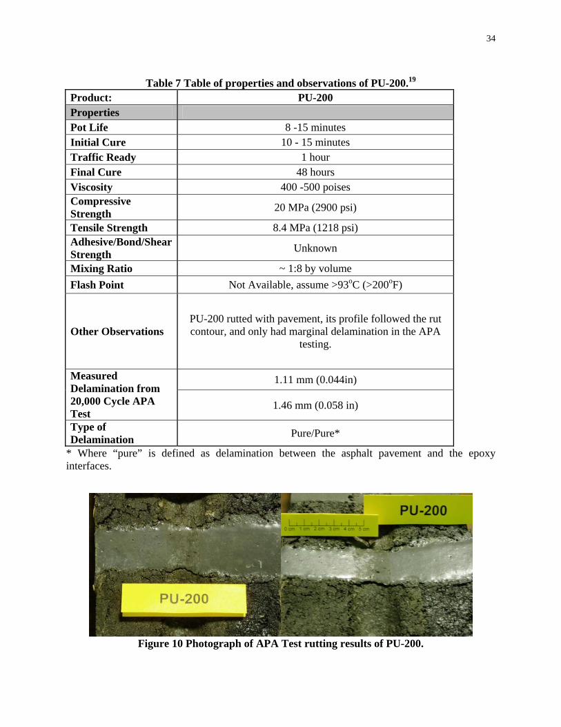
34

Table 7 Table of properties and observations of PU-200.19

Product: PU-200 Properties Pot Life 8 -15 minutes Initial Cure 10 - 15 minutes Traffic Ready 1 hour Final Cure 48 hours Viscosity 400 -500 poises Compressive Strength 20 MPa (2900 psi)

Tensile Strength 8.4 MPa (1218 psi) Adhesive/Bond/Shear Strength Unknown

Mixing Ratio ~ 1:8 by volume Flash Point Not Available, assume >93oC (>200oF)

Other Observations PU-200 rutted with pavement, its profile followed the rut contour, and only had marginal delamination in the APA

testing.

1.11 mm (0.044in) Measured Delamination from 20,000 Cycle APA Test

1.46 mm (0.058 in)

Type of Delamination Pure/Pure*

* Where “pure” is defined as delamination between the asphalt pavement and the epoxy interfaces.

Figure 10 Photograph of APA Test rutting results of PU-200.

35

Table 8 Table of properties and observations of E-Bond G-100.20 Product: E-BOND G-100 Properties Pot Life 30-40 minutes Initial Cure Unknown Traffic Ready 1.5-2 hours (longer below 21oC (70oF)) Final Cure 5 days Viscosity Unknown Compressive Strength 55.1 MPa (8000 psi)

Tensile Strength Unknown Adhesive/Bond/Shear Strength Unknown

Mixing Ratio 1:13 by volume Flash Point >93oC (>200oF)

Other Observations

E-Bond G-100 is very hard (its compressive strength is ~8000 psi higher than typical concrete) and likely to crack when installed in asphalt, five of five samples tested cracked

during APA testing.

0 mm (0 in) Measured Delamination from 20,000 Cycle APA Test

0 mm (0 in)

Type of Delamination None

Figure 11 Photograph of APA Test rutting results of E-Bond G-100.

36

Table 9 Table of properties and observations of ECM P5G.21 Product: ECM P5G Properties Pot Life 5-7 minutes Initial Cure 10-15 minutes Traffic Ready 45-60 minutes Final Cure 20-40 minutes Viscosity 250 poises Compressive Strength 24.7 MPa (3582 psi)

Tensile Strength Unknown Adhesive/Bond/Shear Strength Unknown

Mixing Ratio 1:60 by weight Flash Point <=21oC (<=70oF)

Other Observations

ECM P5G has a flash point of 21oC, toxicity concerns, a sensitive to mixing mistakes due to a high mixing ratio, and

a very short pot life. It also experienced extremely large/severe delamination between epoxy and asphalt in

APA tests.

2.62 mm (0.103 in) Measured Delamination from 20,000 Cycle APA Test

3.57 mm (0.141 in)

Type of Delamination Asphalt Cracking/Asphalt Cracking

Figure 12 Photograph of APA Test rutting results of ECM P5G.

37

Table 10 Table of properties and observations of AS 475.22

Product: AS 475 Properties Pot Life 6-20 minutes Initial Cure Unknown

Traffic Ready Missing tech data (estimate based on final cure 30-40 minutes)

Final Cure 30-40 minutes Viscosity Unknown Compressive Strength Unknown Tensile Strength Unknown Adhesive/Bond/Shear Strength Unknown

Mixing Ratio 1:200 - 1:100 Flash Point 17oC (62.6oF)

Other Observations

AS 475 has a flash point of 17oC making it a potential danger when using in field applications. It also has toxicity

concerns, and very variable pot life due to temp, hardener, and even mixing rate. Sensitive to mixing mistakes due to a

high mixing ratio. All these factors make it an unlikely choice for use.


1.96 mm (0.077 in)

Type of Delamination 50%Pure & 50%Asphalt Crack / 50%Pure & 50%Asphalt Cracking*


Figure 13 Photograph of APA Test rutting results of AS 475.

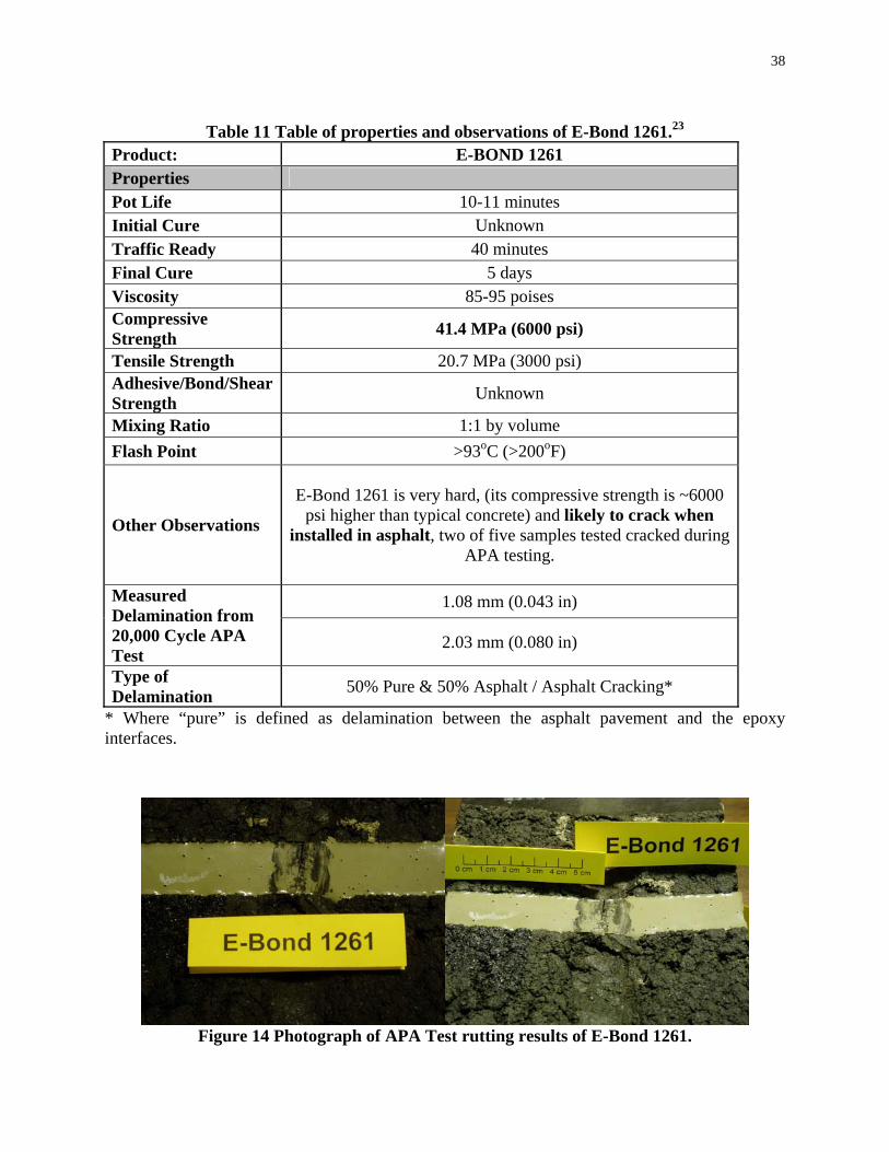
38

Table 11 Table of properties and observations of E-Bond 1261.23

Product: E-BOND 1261 Properties Pot Life 10-11 minutes Initial Cure Unknown Traffic Ready 40 minutes Final Cure 5 days Viscosity 85-95 poises Compressive Strength 41.4 MPa (6000 psi)

Tensile Strength 20.7 MPa (3000 psi) Adhesive/Bond/Shear Strength Unknown


Other Observations

E-Bond 1261 is very hard, (its compressive strength is ~6000 psi higher than typical concrete) and likely to crack when

installed in asphalt, two of five samples tested cracked during APA testing.


2.03 mm (0.080 in)

Type of Delamination 50% Pure & 50% Asphalt / Asphalt Cracking*


Figure 14 Photograph of APA Test rutting results of E-Bond 1261.

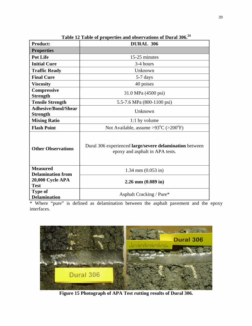
39

Table 12 Table of properties and observations of Dural 306.24

Product: DURAL 306 Properties Pot Life 15-25 minutes Initial Cure 3-4 hours Traffic Ready Unknown Final Cure 5-7 days Viscosity 40 poises Compressive Strength 31.0 MPa (4500 psi)

Tensile Strength 5.5-7.6 MPa (800-1100 psi) Adhesive/Bond/Shear Strength Unknown

Mixing Ratio 1:1 by volume Flash Point Not Available, assume >93oC (>200oF)

Other Observations Dural 306 experienced large/severe delamination between epoxy and asphalt in APA tests.


2.26 mm (0.089 in)

Type of Delamination Asphalt Cracking / Pure*


Figure 15 Photograph of APA Test rutting results of Dural 306.

40


Product: DURAL 340 Properties Pot Life 15-20 minutes (SL version) 10-15 minutes (NL version) Initial Cure 30-40 minutes (SL version) 25-35 minutes (NL version) Traffic Ready 24 hours Final Cure 24 hours Viscosity 40-70 poises Compressive Strength Unknown

Tensile Strength 4.8-5.5 MPa (700-800 psi) Adhesive/Bond/Shear Strength Unknown


Other Observations Dural 340 has a very long wait time prior to being able to open to traffic. Large/severe delamination between epoxy

and asphalt in APA tests.


1.88 mm (0.074 in)



Figure 16 Photograph of APA Test rutting results of Dural 340.

41

Table 14 Table of properties and observations of Bondo 7084.26 Product: BONDO 7084 Properties Pot Life 17-25 minutes Initial Cure 45 minutes Traffic Ready 1 hour Final Cure 1 hour Viscosity Unknown Compressive Strength Unknown

Tensile Strength 17.2 MPa (2500 psi) Adhesive/Bond/Shear Strength 13.8 MPa (2000 psi)


Other Observations Bondo 7084 is very thick and extremely difficult to work

with, rigidity may cause issues if the road ruts, however there was no delamination in APA tests.

0 mm (0in) Measured Delamination from 20,000 Cycle APA Test

0.69 mm (0.027 in)

Type of Delamination None / Asphalt Cracking

Figure 17 Photograph of APA Test rutting results of Bondo 7084.

42

Table 15 Table of properties and observations of MM-80.27

Product: MM-80 Properties Pot Life 15 - 30 minutes Initial Cure 4 - 8 hours Traffic Ready 6 - 12 hours Final Cure Unknown Viscosity Unknown Compressive Strength 10.5 MPa (1530 psi yield)

Tensile Strength 2.8-3.4 MPa (400 - 500 psi) Adhesive/Bond/Shear Strength 1.7 MPa (250 psi) – 2.0 MPa (285 psi)


Other Observations

MM-80 has a long wait time prior to being able to open to traffic. Some delamination in APA but not too severe…this is

typically used in warehouses and other facilities that can be closed for a period of time not necessarily highways. “Not

designed for use in exterior joints (paving etc.)”


1.24 mm (0.049 in)

Type of Delamination Pure / Asphalt Cracking*


Figure 18 Photograph of APA Test rutting results of MM-80.

43

It was originally planned to evaluate Dural 335 along with the other epoxies. However when this material was used, it was found that due to the viscosity it simply flowed into the voids of the asphalt sample. This material was therefore not tested. However, such a material might be practical to augment asphalt segments in the field to make the underlying pavement more durable. In Table 16, the properties for Dural 335 are shown for reference purposes. Since the epoxy has such a low viscosity and can infiltrate the remaining voids in a HMA pavement, this could have a significant impact on the longevity of the surrounding HMA pavement and the adhesion of a WIM sensor assembly to the roadway. Future research is suggested to evaluate the effects of applying Dural 335 after completion of a typical WIM installation. It was suspected that the entire area around the installation would become more rigid and have better durability after a post WIM installation application using Dural 335.


Product: DURAL 335 Properties Pot Life 20-25 minutes Initial Cure 40-50 minutes Traffic Ready - Final Cure - Viscosity 0.8-1.0 poises Compressive Strength 48.3 MPa (7000 psi) – 55.2 MPa (8000 psi)

Tensile Strength 48.3 MPa (7000 psi) – 55.2 MPa (8000 psi) Adhesive/Bond/Shear Strength 12.4 MPa (1800 psi) - 13.8 MPa (2000 psi)


Other Observations Dural 335 is very fluid, normally used to fill cracks and seep into the aggregate structure. This epoxy infiltrated the asphalt

structure and could not be used in the lab APA tests.

N.A Measured Delamination from 20,000 Cycle APA Test

N.A

Type of Delamination N.A

44

A summary of the APA testing can be found in Table 17 along with comments on each epoxy. E-Bond G-100 was discounted because of the longitudinal cracks. AS 475 was discounted primarily because of the delamination; however the low flash point, toxicity, and extremely short pot life should also be mentioned. ECM P5G was discounted primarily because of the sever delamination, low flash point, and longitudinal cracks; however toxicity and tricky mixing ratio should also be mentioned. E-Bond 1261 was discounted because of the longitudinal cracks. Dural 306 and Dural 340 both had significant delamination and transverse cracks, plus Dural 340 has a long 24 hr wait time before traffic ready. Bondo 7084 performed well however it did not mold well to the contour of the rutted pavement and protruded from the sample; it was discounted because of ride quality issues and potential for damage during snow removal; plus it was very difficult to work with. MM-80 also performed well however it was discounted because it has a long 12 hr wait time before traffic ready. Dural 335 was immediately discounted because its viscosity which caused it to infiltrated the voids of the asphalt and seeped away and thus could not be used.

45

Table 17 Summary table of testing conducted on the various epoxies.

Epoxy Type

Samples Tested at

64oC

Visual Delamination &

Cracking Observations

Use Rank* Rigidity Summary/Other

Observations

PU-200 2 Moderate delamination 1.5

Very flexible, rutting closely matched that

of asphalt, and did not create additional epoxy protrusion

Rapid set time, suggested to use

rapidly after mixing

components

E-BOND G-100 5

Five samples (epoxy) cracked longitudinally

1.5 No delamination Longitudinal cracks

ECM P5G 2

Severe delamination,

transverse cracks in asphalt around

epoxy; one sample (epoxy) cracked longitudinally

2 Quite rigid Cures very fast, large variance in

curing time

AS 475 2 Small delamination

and transverse cracks in asphalt

1.5 Quite flexible, rutting closely matched that

of asphalt

Low flash point, toxicity, and tricky mixing

ratio

E-BOND 1261 5

Two samples (epoxy) cracked longitudinally

3 Very rigid, very small deformation

Longitudinal cracks

DURAL 306 3

Three samples had significant

transverse cracks in asphalt

2

Flexible, rutting closely matched that of asphalt, did not create additional epoxy protrusion

Significant delamination

DURAL 340 4 Large/severe

delamination 2 Quite flexible, rutting closely matched that

of asphalt

Long wait until traffic ready

24hrs

BONDO 7084 6 No change 3

Very rigid, minor delamination; asphalt

rutted creating an epoxy protrusion

Protrudes from rutted sample

MM-80 2

Small delamination in one case; second

case minor delamination

2.5 Long wait until

traffic ready 12hrs

* Use Ranking: 1, 2, and 3 see below. 1-Easy to use/handle – viscous, similar to a sand/water mix 2-Normal to use/handle – moderate viscosity, between honey and tar 3-Difficult to use/handle - sticky, very dense like tar

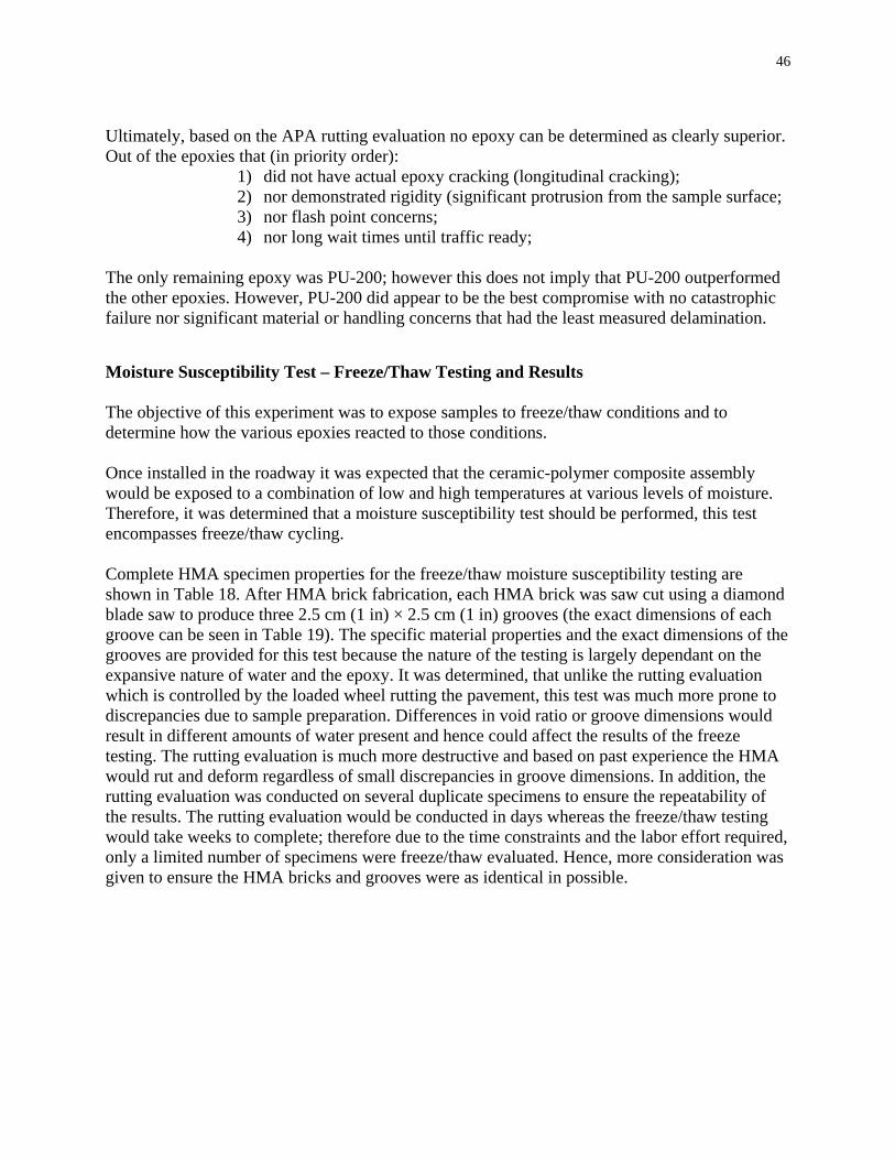
46

Ultimately, based on the APA rutting evaluation no epoxy can be determined as clearly superior. Out of the epoxies that (in priority order):

1) did not have actual epoxy cracking (longitudinal cracking); 2) nor demonstrated rigidity (significant protrusion from the sample surface; 3) nor flash point concerns; 4) nor long wait times until traffic ready;

The only remaining epoxy was PU-200; however this does not imply that PU-200 outperformed the other epoxies. However, PU-200 did appear to be the best compromise with no catastrophic failure nor significant material or handling concerns that had the least measured delamination. Moisture Susceptibility Test – Freeze/Thaw Testing and Results The objective of this experiment was to expose samples to freeze/thaw conditions and to determine how the various epoxies reacted to those conditions. Once installed in the roadway it was expected that the ceramic-polymer composite assembly would be exposed to a combination of low and high temperatures at various levels of moisture. Therefore, it was determined that a moisture susceptibility test should be performed, this test encompasses freeze/thaw cycling. Complete HMA specimen properties for the freeze/thaw moisture susceptibility testing are shown in Table 18. After HMA brick fabrication, each HMA brick was saw cut using a diamond blade saw to produce three 2.5 cm (1 in) × 2.5 cm (1 in) grooves (the exact dimensions of each groove can be seen in Table 19). The specific material properties and the exact dimensions of the grooves are provided for this test because the nature of the testing is largely dependant on the expansive nature of water and the epoxy. It was determined, that unlike the rutting evaluation which is controlled by the loaded wheel rutting the pavement, this test was much more prone to discrepancies due to sample preparation. Differences in void ratio or groove dimensions would result in different amounts of water present and hence could affect the results of the freeze testing. The rutting evaluation is much more destructive and based on past experience the HMA would rut and deform regardless of small discrepancies in groove dimensions. In addition, the rutting evaluation was conducted on several duplicate specimens to ensure the repeatability of the results. The rutting evaluation would be conducted in days whereas the freeze/thaw testing would take weeks to complete; therefore due to the time constraints and the labor effort required, only a limited number of specimens were freeze/thaw evaluated. Hence, more consideration was given to ensure the HMA bricks and grooves were as identical in possible.

47

Table 18 Properties of HMA Bricks used for the Moisture Susceptibility Testing

A B C D

P 1 2 .5 F + 2 v ib ra to ry b r ic k 4 .7 8 2 .5P 1 2 .5 F + 3 v ib ra to ry b r ic k 4 .7 8 1 .5P 1 2 .5 F + 6 v ib ra to ry b r ic k 4 .7 8 2 .5

E F

P 1 2 .5 F + 2 2 .9 2 5 2 .6 9 3P 1 2 .5 F + 3 2 .9 2 5 2 .6 9 3P 1 2 .5 F + 6 2 .9 2 5 2 .6 9 3

G H I

P 1 2 .5 F + 2 7 2 2 4 .0 7 3 3 5 .7 4 3 4 9 .2P 1 2 .5 F + 3 7 2 3 2 .9 7 3 4 6 .7 4 3 6 6 .1P 1 2 .5 F + 6 7 2 2 6 .2 7 3 1 7 .2 4 3 3 3 .4

J K L

P 1 2 .5 F + 2 2 9 8 6 .5 2 .4 1 9 9 5 .3P 1 2 .5 F + 3 2 9 8 0 .6 2 .4 2 7 9 5 .3P 1 2 .5 F + 6 2 9 8 3 .8 2 .4 2 2 9 5 .3

M N O

P 1 2 .5 F + 2 1 5 0 .9 1 0 .2 2 1 .2P 1 2 .5 F + 3 1 5 1 .4 9 .9 2 0 .9P 1 2 .5 F + 6 1 5 1 .1 1 0 .1 2 1 .1

P Q

P 1 2 .5 F + 2 5 2 .0 2 9 5P 1 2 .5 F + 3 5 2 .8 2 9 5P 1 2 .5 F + 6 5 2 .3 2 9 5

V o lu m e o f S p e c im e n

(H - I )

S p . G ra v ity o f S p e c .

S p e c im e n ID T o ta l A .C . (% ) T h ic k n e s s (m m )

W e ig h t o f S p e c im e n in G ra m s

In A ir S .S .D .

A g g . G s b

T e m p . o f M ix a t C o m p a c t io n ( o F )

V F A %

[ (O - N ) / O ] * 1 0 0

(G / J ) (1 0 0 - C )

(K * 6 2 .4 ) [1 0 0 * { (F - K ) / F } ] [1 0 0 - (K * L / E ) ]

% A g g .

U n it W t . (p c f ) % A ir V o id s V M A %

P ro je c t: A P A E v a lu a t io n o f V a r io u s E p o x y R e s in s fo r U s e w ith W .I.M . S e n s o rsA s p h a lt P a v e m e n t S p e c im e n W o rk s h e e t

M ix T y p e : 1 2 .5 m m f in e (1 /2 in c h ) w ith 7 % v o id s

(B u lk S p . G r . o f A g g re g a te s )

G m m

(M a x . S p . G r . )

In W a te r (@ 4 m in .)

S a m p le T y p e

48

Table 19 Calculation of Voids After Grooves Were Saw Cut.

49

To conduct the evaluation AASHTO T-283 “Resistance of Compacted Bituminous Mixture to Moisture-Induced Damage” was used as a model for the testing.29 The test was modified to meet the needs of evaluating the bond between the various epoxies and asphalt. The most significant deviation of the test method from the official procedure was that; the HMA brick was used instead of a core sample and that an indirect tensile test was not conducted. The goal of the testing was to evaluate the epoxy bonding and durability due to moisture damage for asphalt mixtures. The AASHTO T-283 test was used to evaluate the effects of saturations and accelerated water conditioning on the samples. The test consisted of saturating the samples to between 55%-80%. To achieve this level of saturation, vacuum saturation was used. The pump and vacuum gage from the Rice test were used with a 5 gallon container to create the vacuum container. A vacuum of 100 kPa (15 psi) was achieved within the container. All testing was conducted at room temperature.

Figure 19 Photograph of vacuum container with vacuum pump and gage.

The vacuum container, as shown in Figure 19, was then filled with water to a level that when the sample was placed in the container the sample was completely covered by approximately 2.54 cm (1 in) of water. Salt was then added to the water, as shown in Figure 20, and the solution was then mixed well to form a brine solution to mimic the harshest field conditions. For example, during winter months when salt is frequently used on the roadway this can significantly degrade asphalt bonding. Normally, durability testing is done with distilled water but this approach was meant as a torture test to accelerate potential damage.

50

Figure 20 Addition of salt to form brine solution to ensure test would be performed under

worst case environmental effects.

The saturated surface-dry mass of each sample was determined and is shown in Figure 21. Each brick was then subjected to vacuum conditioning for 15 minutes. The vacuum was then removed and the samples were allowed to sit in the solution for another 5 minutes. The samples were then removed from the vacuum container and the saturated surface-dry mass was re-measured and compared to the original measurement. The saturation for two HMA bricks was 62% and for the HMA third brick it was 66%. Therefore, within an acceptable tolerance of 55-80% according to T-283, all the samples had roughly the sample level of saturation and the testing was continued.29

Figure 21 Weighing of samples to determine saturated surface dry (SSD) weight.

The samples were then tightly wrapped in plastic (Saran wrap™) film to maintain the level of saturation. Then the samples were placed into plastic bags with an additional 10 ml (0.33 oz) of water and the bags were sealed, as shown in Figure 22. This completed the preconditioning of the samples, such that the freeze/thaw cycle testing could start.

51

Figure 22 Photograph of the three bricks, with three separate epoxy samples each wrapped

in saran wrap and sealed in plastic bags. Each freeze/thaw cycle consisted of exposing the sample to the temperature of –18oC ±3 degrees (0oF ±5 degrees) for 16 hours and then removing them from the freezer, as shown in Figure 23, then exposing the samples to room temperature for another 8 hours. Each complete freeze/thaw cycle took 24 hours to complete.

Figure 23 Photograph of samples in freezer unit.

The goal of the moisture susceptibility (freeze/thaw) testing was to determine after how many cycles would a noticeable delamination occur between the asphalt and the epoxies/acrylics? The samples were tested for fifty freeze/thaw cycles (55 days of testing). Since no delamination was

52

observed after nearly two months of Freeze/Thaw testing, the test was stopped and it was concluded that the results were inconclusive.

Material Compatibility Analysis Since the results of the Freeze/Thaw testing were largely inconclusive a second set of tests were conducted to evaluate the thermal expansion and elastic modulus of the various epoxies. Each epoxy was evaluated and compared to asphalt to try draw a correlation between delamination results derived from the earlier APA rut testing and the epoxy material thermal properties.

Thermal Expansion Analysis Since the results of the Freeze/Thaw testing were largely inconclusive, a second test was conducted to evaluate the thermal expansion properties of the epoxy in comparison to asphalt. Samples were placed in a freezer for 24hrs and the length of each epoxy groove was measured. Then the samples were placed in an oven for 24hrs and the lengths were once again measured. The results of the test can be seen in Table 20 and Table 21. From the results it can be observed that the some of the epoxies did experience significant dimensional change as a result of temperature changes. In theory, this is important because in actual field conditions the closer the epoxy matches the expansion properties of asphalt pavement the less probability of delamination occurring or water infiltration. Either of which could result in a faster failure due to debonding or delamination occurring between the epoxy and the HMA pavement.

53

Table 20 Lengths of epoxy samples under cold conditioning.

-18 oC Epoxies ECM P5G AS 475 E-Bond 1261

Sample Label F+3

Trial #1 Length (mm) 125.5 125.91 127.16

Trial #2 Length (mm) 125.34 125.86 127.37

Sample Label F+2 E-Bond G-100 Bondo 7084 PU-200

Trial #1 Length (mm) 126.16 126.06 127.98

Trial #2 Length (mm) 126.1 125.98 127.89

Sample Label F+6 Dural 340 Dural 306 MM-80

Trial #1 Length (mm) 127.52 126.69 126.71

Trial #2 Length (mm) 127.17 126.76 126.79

Sample Label Asphalt Trial #1 Length (mm) 124.99 125.1

54

Table 21 Lengths of epoxy samples under hot conditioning.

68 oC Epoxies ECM P5G AS 475 E-Bond 1261

Sample Label F+3

Trial #1 Length (mm) 125.75 126.64 128.13

Trial #2 Length (mm) 125.97 126.53 128.77

Sample Label F+2 E-Bond G-

100 Bondo 7084 PU-200

Trial #1 Length (mm) 126.77 126.93 128.86

Trial #2 Length (mm) 126.96 127.41 129.45

Sample Label F+6 Dural 340 Dural 306 MM-80

Trial #1 Length (mm) 128.25 127.45 127.15

Trial #2 Length (mm) 129.37 128.33 128.84

Sample Label Asphalt

Trial #1 Length (mm) 125.21 125.33 The amount of dimensional change that any material will undergo due to temperature is usually represented by the Coefficient of Thermal Expansion. The Coefficient of Thermal Expansion describes the change in length of a member per unit length per degree temperature change. The Coefficient of Thermal Expansion can be estimated by calculating the (total change in length) / ((change in temperature) * length). Typical thermal coefficient values of HMA vary from 2.1E-5 to 6.5E-5/oC; the results of the epoxy analysis can be seen in Table 22. The actual measurement of the HMA samples’ Coefficient of Thermal Expansion closely matched this range; thus verifying the initial validity of this experiment. From this table there were four epoxies, shown in ‘underline’, that fall within this range, they were ECM P5G, AS 475, E-Bond G-100, and MM-80. However, with exception of E-Bond G-100 which had no delamination observed but did experienced longitudinal cracking of the epoxy and was considered a failure for that reason; the other three samples have significant delamination. The ECM P5G and the E-Bond G-100 were at the extreme opposite ends of the spectrum in relation to the measured delamination, but they had similar thermal expansion coefficients. Therefore, either this test was flawed (possibly due to the

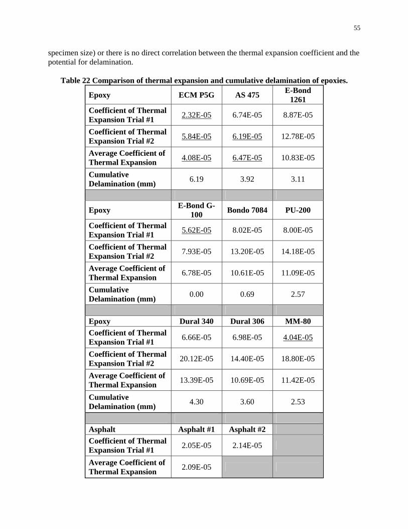
55

specimen size) or there is no direct correlation between the thermal expansion coefficient and the potential for delamination.

Table 22 Comparison of thermal expansion and cumulative delamination of epoxies.

Epoxy ECM P5G AS 475 E-Bond 1261

Coefficient of Thermal Expansion Trial #1 2.32E-05 6.74E-05 8.87E-05


Average Coefficient of Thermal Expansion 4.08E-05 6.47E-05 10.83E-05

Cumulative Delamination (mm) 6.19 3.92 3.11

Epoxy E-Bond G-100 Bondo 7084 PU-200





Epoxy Dural 340 Dural 306 MM-80 Coefficient of Thermal Expansion Trial #1 6.66E-05 6.98E-05 4.04E-05




Asphalt Asphalt #1 Asphalt #2 Coefficient of Thermal Expansion Trial #1 2.05E-05 2.14E-05

Average Coefficient of Thermal Expansion 2.09E-05

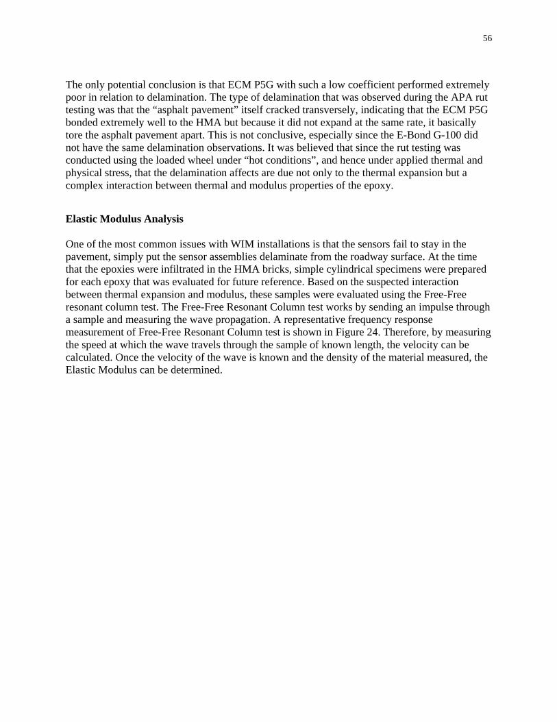
56

The only potential conclusion is that ECM P5G with such a low coefficient performed extremely poor in relation to delamination. The type of delamination that was observed during the APA rut testing was that the “asphalt pavement” itself cracked transversely, indicating that the ECM P5G bonded extremely well to the HMA but because it did not expand at the same rate, it basically tore the asphalt pavement apart. This is not conclusive, especially since the E-Bond G-100 did not have the same delamination observations. It was believed that since the rut testing was conducted using the loaded wheel under “hot conditions”, and hence under applied thermal and physical stress, that the delamination affects are due not only to the thermal expansion but a complex interaction between thermal and modulus properties of the epoxy. Elastic Modulus Analysis One of the most common issues with WIM installations is that the sensors fail to stay in the pavement, simply put the sensor assemblies delaminate from the roadway surface. At the time that the epoxies were infiltrated in the HMA bricks, simple cylindrical specimens were prepared for each epoxy that was evaluated for future reference. Based on the suspected interaction between thermal expansion and modulus, these samples were evaluated using the Free-Free resonant column test. The Free-Free Resonant Column test works by sending an impulse through a sample and measuring the wave propagation. A representative frequency response measurement of Free-Free Resonant Column test is shown in Figure 24. Therefore, by measuring the speed at which the wave travels through the sample of known length, the velocity can be calculated. Once the velocity of the wave is known and the density of the material measured, the Elastic Modulus can be determined.

57

Figure 24 Free-Free Resonant Column tests results, frequency response of PU-200.

The summary of results of the test can be seen in Table 23 and Figure 25. HMA has a typical range of 14,000 MPa (2,000,000 psi) at 0oC (32oF); 3,500 MPa (500,000 psi) at 21oC (70oF); and 150 MPa (20,000 psi) at 49oC (120oF).30 Ideally, the roadway epoxy properties should match that of the HMA pavement, however based on the testing data all the epoxies have higher modulus than HMA at all temperatures. As a vehicle tire applies a load on the roadway, it goes through a complex interaction of stress and strains both in a longitudinal as well as transverse directions. If the epoxy is significantly harder or softer than the roadway material this can result in amplified loading effects. These effects can cause the roadway material to pull away from the epoxy leading to delamination or it can result in additional compression that will cause fatigue cracking of the pavement. Regardless of the mechanism, the result is inevitably failure of the sensor.

58

Table 23 Comparison of Elastic Modulus of epoxies to asphalt.

59

Elastic Modulus of Roadway Epoxies

0

2

4

6

8

10

12

0 10 20 30 40 50 60 70Temperature (C)

Mod

ulus

N/m

2 x 1

010

PU-200

AS 475

MM-80

Dural 306

E-Bond 1261

E-Bond G-100

Dural 340

ECM P5G

Bondo 7084

Figure 25 Comparison of Elastic Modulus.

In reviewing the epoxy properties it was decided to exclude the two epoxies, E-Bond G100 and E-Bond 1261, which cracked during the rutting evaluation from further consideration. Also, Bondo 7084 was eliminated due to is high modulus results, as well as its inability to conform to the pavement surface during the rutting evaluation. The above materials were eliminated from Figure 25 and plotted along with HMA modulus in Figure 26. HMA has a typical range of 14,000 MPa (2,000,000 psi) at 0oC (32oF); 3,500 MPa (500,000 psi) at 21oC (70oF); and 150 MPa (20,000 psi) at 49oC (120oF).31 Ideally, the roadway epoxy properties should match that of the HMA pavement, however based on the testing data all the epoxies have higher modulus than HMA at all temperatures. At higher temperatures all the six remaining epoxies fall within the HMA comparative zone of elastic modulus. However at 25oC (77oF) only the PU-200 and the Dural 306 fall within this zone; whereas at 4oC (40oF) only PU-200 remains within this HMA comparative zone of Elastic Modulus.

60

Zone of Elastic Modulus Close to that of HMA Pavement in Relation to the Remaining Roadway Epoxies

0

1

2

3

4

5

0 10 20 30 40 50 60 70Temperature (C)

Mod

ulus

N/m

2 x

1010

HMA Pvmnt.

PU-200

AS 475

MM-80

Dural 306

Dural 340

ECM P5G

Figure 26 Zone of Elastic Modulus close to that of HMA pavement in relation to the

remaining roadway epoxies The delamination results of the remaining six epoxies were then plotted against the ratio of Coefficient of Thermal Expansion and ratio x10000 of elastic modulus at ~60oC of the epoxies to HMA. The elastic modulus ratio had to be multiplied by 10,000 to normalize the data and allow for plotting of the data on the same graph. For simplicity reasons the epoxies are shown from left to right in order of least to most cumulative delamination measured during the rut evaluation. The results of this analysis can be seen in Figure 27. It is believed that the epoxy performance can be predicted by complex interaction between these factors and the compressive strength (not shown here for simplicity reasons). It was assumed, that the higher the modulus the more likely the epoxy was to crack, however the compressive strength must be taken into consideration as well. Therefore, there must exist some upper level threshold for the material properties to “not exceed” when evaluating performance. In addition as a general rule, it was shown that the higher these two combined ratios were, the less delamination occurred. This was true even for the high modulus materials such as E-Bond G-100 and Bondo 7084, even though they were eliminated from consideration for other reasons. MM-80 is the exception to this rule, it had lower ratios and a smaller delamination. However, given that MM-80 and PU-200 had very similar delamination measurements; but considering that MM-80 according to the manufactured is “not designed for use in exterior joints (paving etc.)”27 it was for this reason that MM-80 was discounted as well,

HMA Pavement Zone of Comparative Analysis

61

and PU-200 selected for all future testing. Dural 306 was a close second, however it did experience a higher measured cumulative delamination during the rut evaluation.

Comparison of Cumulative Delamination of Various Epoxies to the Ratio of Coefficient of Thermal Expansion and Ratio of Elastic Modulus at ~60oC of Epoxies to HMA

0

1

2

3

4

5

6

7

E-BONDG-100

BONDO7084

MM-80 PU 200 E-BOND1261

DURAL 306

AS 475 DURAL340

ECM P5G

Epoxy Type

Del

amin

atio

n (m

m

0.0

0.5

1.0

1.5

2.0

2.5

3.0

3.5

4.0

4.5

Rat

io o

f Sel

ecte

d M

ater

ial

Prop

erty

of E

poxy

to H

MA

Cumulative Delamination (mm)Ratio of Average Coefficient of Thermal Expansion (Epoxy to HMA)Ratiox10000 of Elastic Modulus at ~60oC (Epoxy to HMA)

Figure 27 Comparison of cumulative delamination of various epoxies to the ratio of Coefficient of Thermal Expansion and ratiox10000 of Elastic Modulus at ~60oC of epoxies

to HMA.

Fabrication and Testing of Revised Prototype The final sensor design is very similar in appearance to the previous version with one significant exception; the encapsulating epoxy. The new sensor was fabricated using the dice and fill technique with a stiff polymer material used to infiltrate the ceramic. As in the previous designs of the sensor, the composite was encapsulated in an elastomeric block of highway grade epoxy. However, it was determined that the G-100 epoxy used to encapsulate the sensor was significantly harder than needed and the cure time was lengthy. Instead PU-200 epoxy was selected for encapsulating the sensor. None of the evaluated epoxies experienced any delamination during the freeze-thaw evaluation. The PU-200 epoxy, summary of properties can be found in Table 24, rutted with the pavement and only had marginal delamination during the APA rutting evaluation tests. It also had an initial cure time of less than 20 minutes, traffic ready in one (1) hour, and a final cure in 48 hrs; making it an excellent choice for quick installations.

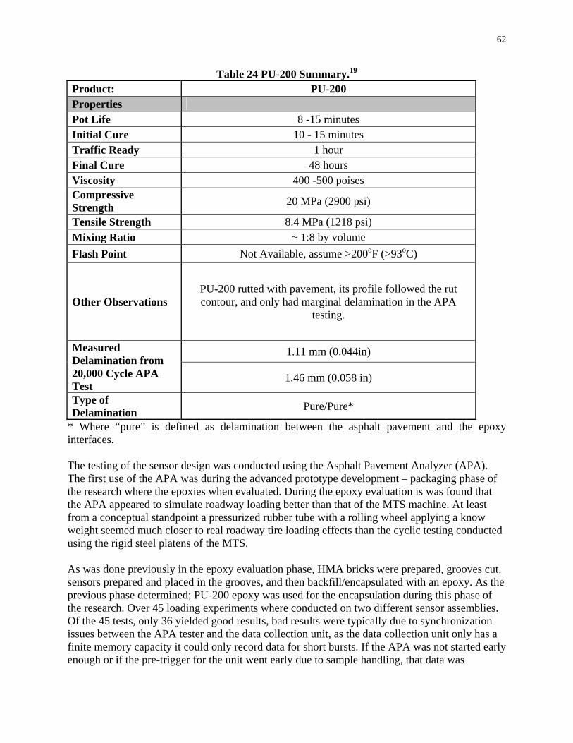
62

Table 24 PU-200 Summary.19 Product: PU-200 Properties Pot Life 8 -15 minutes Initial Cure 10 - 15 minutes Traffic Ready 1 hour Final Cure 48 hours Viscosity 400 -500 poises Compressive Strength 20 MPa (2900 psi)

Tensile Strength 8.4 MPa (1218 psi) Mixing Ratio ~ 1:8 by volume Flash Point Not Available, assume >200oF (>93oC)

Other Observations PU-200 rutted with pavement, its profile followed the rut contour, and only had marginal delamination in the APA

testing.

1.11 mm (0.044in) Measured Delamination from 20,000 Cycle APA Test

1.46 mm (0.058 in)


* Where “pure” is defined as delamination between the asphalt pavement and the epoxy interfaces. The testing of the sensor design was conducted using the Asphalt Pavement Analyzer (APA). The first use of the APA was during the advanced prototype development – packaging phase of the research where the epoxies when evaluated. During the epoxy evaluation is was found that the APA appeared to simulate roadway loading better than that of the MTS machine. At least from a conceptual standpoint a pressurized rubber tube with a rolling wheel applying a know weight seemed much closer to real roadway tire loading effects than the cyclic testing conducted using the rigid steel platens of the MTS. As was done previously in the epoxy evaluation phase, HMA bricks were prepared, grooves cut, sensors prepared and placed in the grooves, and then backfill/encapsulated with an epoxy. As the previous phase determined; PU-200 epoxy was used for the encapsulation during this phase of the research. Over 45 loading experiments where conducted on two different sensor assemblies. Of the 45 tests, only 36 yielded good results, bad results were typically due to synchronization issues between the APA tester and the data collection unit, as the data collection unit only has a finite memory capacity it could only record data for short bursts. If the APA was not started early enough or if the pre-trigger for the unit went early due to sample handling, that data was

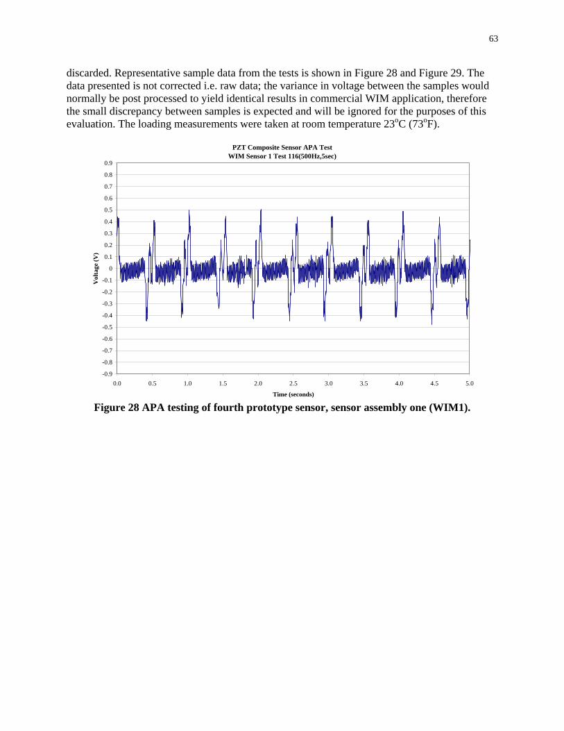
63

discarded. Representative sample data from the tests is shown in Figure 28 and Figure 29. The data presented is not corrected i.e. raw data; the variance in voltage between the samples would normally be post processed to yield identical results in commercial WIM application, therefore the small discrepancy between samples is expected and will be ignored for the purposes of this evaluation. The loading measurements were taken at room temperature 23oC (73oF).

PZT Composite Sensor APA TestWIM Sensor 1 Test 116(500Hz,5sec)

-0.9

-0.8

-0.7

-0.6

-0.5

-0.4

-0.3

-0.2

-0.1

0

0.1

0.2

0.3

0.4

0.5

0.6

0.7

0.8

0.9

0.0 0.5 1.0 1.5 2.0 2.5 3.0 3.5 4.0 4.5 5.0

Time (seconds)

Vol

tage

(V)

Figure 28 APA testing of fourth prototype sensor, sensor assembly one (WIM1).

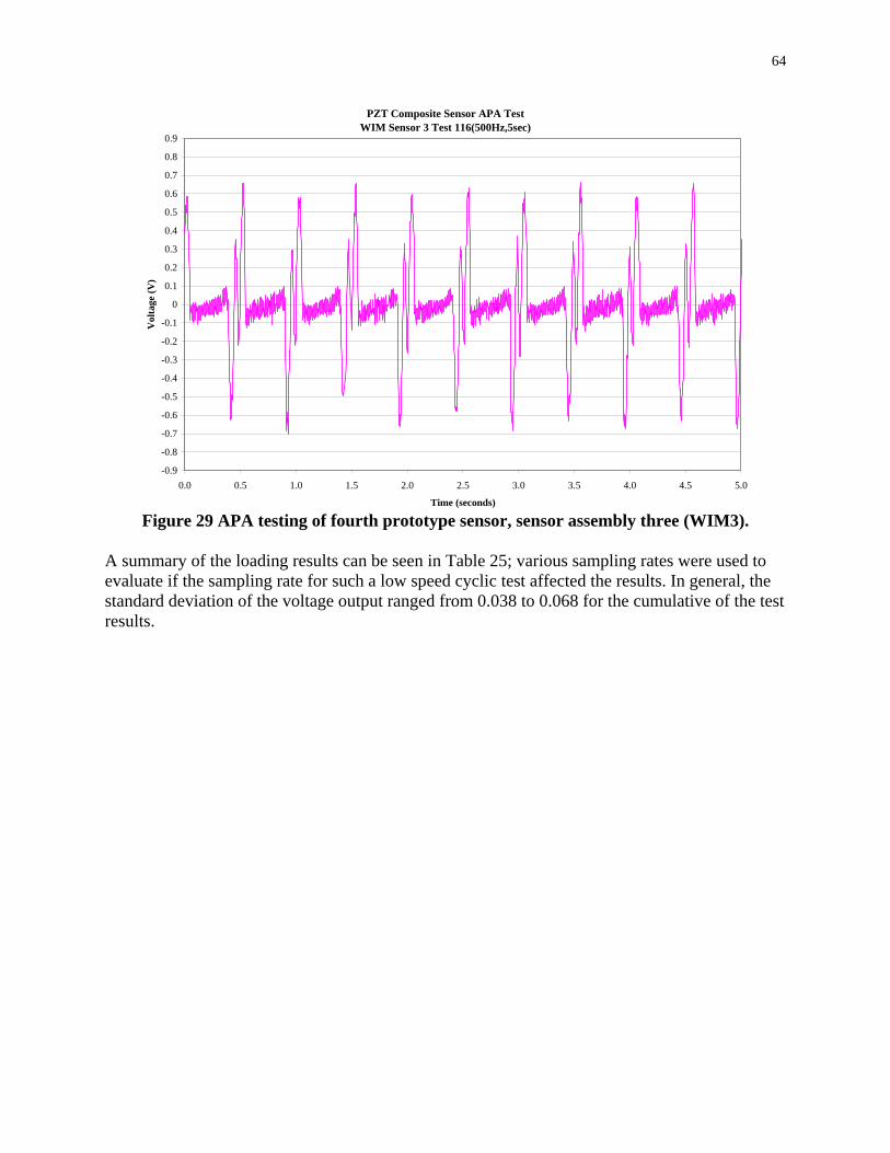
64

PZT Composite Sensor APA TestWIM Sensor 3 Test 116(500Hz,5sec)

-0.9

-0.8

-0.7

-0.6

-0.5

-0.4

-0.3

-0.2

-0.1

0

0.1

0.2

0.3

0.4

0.5

0.6

0.7

0.8

0.9

0.0 0.5 1.0 1.5 2.0 2.5 3.0 3.5 4.0 4.5 5.0

Time (seconds)

Vol

tage

(V)

Figure 29 APA testing of fourth prototype sensor, sensor assembly three (WIM3).

A summary of the loading results can be seen in Table 25; various sampling rates were used to evaluate if the sampling rate for such a low speed cyclic test affected the results. In general, the standard deviation of the voltage output ranged from 0.038 to 0.068 for the cumulative of the test results.

65

Table 25 Table summarizing APA loading results of PZT composite Sensor One and Sensor Three.

Number Test Sampling rate DurationNegative Positive Negative Positive

1 99 1000 5 -0.57084 0.53709 -0.74752 0.827422 100 1000 5 -0.57440 0.53711 -0.76262 0.830073 102 1000 5 -0.50248 0.54865 -0.69602 0.844274 103 1000 5 -0.57910 0.54687 -0.74414 0.823255 106 500 5 -0.47169 0.46387 -0.70313 0.659206 109 500 5 -0.48146 0.49219 -0.70803 0.669937 110 500 5 -0.45606 0.48145 -0.70900 0.674818 111 500 5 -0.37696 0.40723 - -9 112 500 5 -0.39065 0.41018 -0.63282 0.6074210 113 500 5 -0.38575 0.40627 -0.64259 0.6074211 115 800 3 -0.39652 0.39846 -0.63086 0.6172012 116 500 5 -0.40305 0.43058 -0.58860 0.5983713 117 500 5 -0.44390 0.44745 -0.64365 0.6276714 118 500 5 -0.42677 0.44630 -0.64551 0.6132815 119 800 3 -0.44728 0.44340 -0.64260 0.6386616 120 800 3 -0.44142 0.46290 -0.66406 0.6250017 121 800 3 -0.39878 0.40040 -0.56313 0.5403718 122 100 5 -0.41310 0.42481 -0.62891 0.5908019 127 500 5 -0.4561 0.4688 -0.6836 0.662120 128 500 5 -0.4590 0.4834 -0.6699 0.646521 129 500 5 -0.4629 0.4625 -0.6846 0.663222 130 200 12.5 -0.4564 0.4534 -0.6677 0.643023 131 200 12.5 -0.4551 0.4598 -0.6621 0.638724 132 200 12.5 -0.4520 0.4555 -0.6613 0.645325 133 400 6.3 -0.46289 0.4746 -0.66992 0.6630926 134 400 6.3 -0.44728 0.47658 -0.64357 0.6591727 135 400 6.3 -0.47072 0.47655 -0.66994 0.6552728 136 600 4.2 -0.4709 0.4731 -0.6717 0.652129 137 600 4.2 -0.4356 0.4434 -0.6387 0.621130 138 600 4.2 -0.4737 0.4785 -0.6738 0.660231 139 800 3 -0.4743 0.4716 -0.6780 0.658532 140 800 3 -0.4623 0.4668 -0.6641 0.654333 141 800 3 -0.4715 0.4702 -0.6682 0.657134 142 1000 2.5 -0.4668 0.4688 -0.6778 0.659935 143 1000 2.5 -0.4746 0.4766 -0.6758 0.668036 145 1000 2.5 -0.4568 0.4678 -0.6576 0.6660

Average -0.4575 0.4642 -0.6678 0.6620Standard deviation 0.0466 0.0375 0.0394 0.0677

WIM 1 WIM 3

Each sampling rate was then grouped and summarized in Table 26. By keeping the same sampling rate but comparing the length of the test, for example 1000 Hz at 2.5s and 5s, for roughly the same number of tests; it was found that the longer the test the more variation in the sample. However, in comparison to earlier tests (i.e. 500 Hz and 5s) the variation was almost identical; therefore it can be determined that any cyclic test less than 2.5s will yield far too much variation because the test length is not long enough to provide an adequate data set to produce a realistic average result. Also by ignoring any data less than 5s sample collection time, and plotting the results (Figure 30), it can be seen that there is roughly a 25% increase in voltage

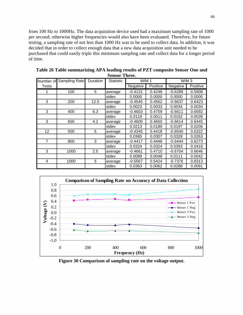
66

from 100 Hz to 1000Hz. The data acquisition device used had a maximum sampling rate of 1000 per second; otherwise higher frequencies would also have been evaluated. Therefore, for future testing, a sampling rate of not less than 1000 Hz was to be used to collect data. In addition, it was decided that in order to collect enough data that a new data acquisition unit needed to be purchased that could easily triple this minimum sampling rate and collect data for a longer period of time.

Table 26 Table summarizing APA loading results of PZT composite Sensor One and

Sensor Three. Sampling Rate Duration Statistic

Negative Positive Negative Positive1 100 5 average -0.4131 0.4248 -0.6289 0.5908

stdev 0.0000 0.0000 0.0000 0.00003 200 12.5 average -0.4545 0.4562 -0.6637 0.6423

stdev 0.0023 0.0033 0.0034 0.00343 400 6.3 average -0.4603 0.4759 -0.6611 0.6592

stdev 0.0119 0.0011 0.0152 0.00393 600 4.2 average -0.4600 0.4650 -0.6614 0.6445

stdev 0.0213 0.0189 0.0197 0.020612 500 5 average -0.4345 0.4418 -0.6540 0.6322

stdev 0.0365 0.0307 0.0328 0.02637 800 3 average -0.4417 0.4448 -0.6444 0.6273

stdev 0.0324 0.0324 0.0393 0.04163 1000 2.5 average -0.4661 0.4710 -0.6704 0.6646

stdev 0.0089 0.0048 0.0111 0.00424 1000 5 average -0.5567 0.5424 -0.7376 0.8313

stdev 0.0363 0.0062 0.0288 0.0091

WIM 1 WIM 3Number of Tests

Comparison of Sampling Rate on Accuracy of Data Collection

-1.0-0.8-0.6-0.4-0.20.00.20.40.60.81.0

0 200 400 600 800 1000Frequency (Hz)

Vol

tage

(V) Sensor 1 Pos

Sensor 1 NegSensor 3 PosSensor 3 Neg

Figure 30 Comparison of sampling rate on the voltage output.

67

Conclusions Advanced Prototype Development Packaging (Epoxy Selection) Based on the results of the advanced prototype development packaging (epoxy selection) effort the following can be concluded:

• Based on the APA rutting evaluation no epoxy can be determined as clearly

superior. Ranking was done considering the following priorities: 1) did not have actual epoxy cracking (longitudinal cracking); 2) nor demonstrated rigidity (significant protrusion from the sample surface; 3) nor flash point concerns; 4) nor long wait times until traffic ready;

PU-200 appeared to be the best compromise based on the APA rut testing, with no catastrophic failure nor significant material or handling concerns that had the least measured delamination. However this does not mean that PU-200 truly outperformed the other epoxies.

• From the APA rut test, it was determined that the G-100 epoxy used to originally encapsulate the sensor was significantly harder than needed and the cure time was lengthy. Instead PU-200 was selected for encapsulating all future sensors for the remainder of the research effort.

• Freeze/thaw testing results were inconclusive. None of the evaluated epoxies experienced any delamination during the freeze/thaw evaluation.

• The Coefficient of Thermal Expansion analysis showed no direct correlation between the thermal expansion coefficient and the potential for delamination.

• Elastic modulus testing revealed that all the epoxies have higher modulus than HMA at all temperatures.

• It was assumed, that the higher the modulus the more likely the epoxy was to crack, however the compressive strength must be taken into consideration as well. Therefore, there must exist some upper level threshold for the material properties to “not exceed” when evaluating performance.

• In addition as a general rule, it was shown that the higher the ratios of Elastic Modulus and Coefficient of Thermal Expansion of epoxy to HMA were, the less delamination occurred. This was true even for the high modulus materials such as E-Bond G-100 and Bondo, even though they were eliminated from consideration for other reasons.

• Based on these findings PU-200 was selected for all future testing. Dural 306 was a close second, however it did experience a higher measured cumulative delamination during the rut evaluation.

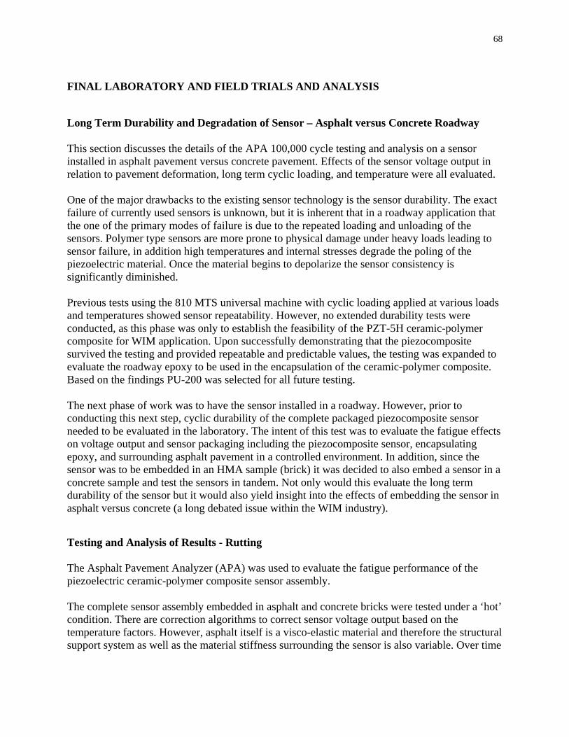
68

FINAL LABORATORY AND FIELD TRIALS AND ANALYSIS

Long Term Durability and Degradation of Sensor – Asphalt versus Concrete Roadway This section discusses the details of the APA 100,000 cycle testing and analysis on a sensor installed in asphalt pavement versus concrete pavement. Effects of the sensor voltage output in relation to pavement deformation, long term cyclic loading, and temperature were all evaluated. One of the major drawbacks to the existing sensor technology is the sensor durability. The exact failure of currently used sensors is unknown, but it is inherent that in a roadway application that the one of the primary modes of failure is due to the repeated loading and unloading of the sensors. Polymer type sensors are more prone to physical damage under heavy loads leading to sensor failure, in addition high temperatures and internal stresses degrade the poling of the piezoelectric material. Once the material begins to depolarize the sensor consistency is significantly diminished. Previous tests using the 810 MTS universal machine with cyclic loading applied at various loads and temperatures showed sensor repeatability. However, no extended durability tests were conducted, as this phase was only to establish the feasibility of the PZT-5H ceramic-polymer composite for WIM application. Upon successfully demonstrating that the piezocomposite survived the testing and provided repeatable and predictable values, the testing was expanded to evaluate the roadway epoxy to be used in the encapsulation of the ceramic-polymer composite. Based on the findings PU-200 was selected for all future testing. The next phase of work was to have the sensor installed in a roadway. However, prior to conducting this next step, cyclic durability of the complete packaged piezocomposite sensor needed to be evaluated in the laboratory. The intent of this test was to evaluate the fatigue effects on voltage output and sensor packaging including the piezocomposite sensor, encapsulating epoxy, and surrounding asphalt pavement in a controlled environment. In addition, since the sensor was to be embedded in an HMA sample (brick) it was decided to also embed a sensor in a concrete sample and test the sensors in tandem. Not only would this evaluate the long term durability of the sensor but it would also yield insight into the effects of embedding the sensor in asphalt versus concrete (a long debated issue within the WIM industry). Testing and Analysis of Results - Rutting The Asphalt Pavement Analyzer (APA) was used to evaluate the fatigue performance of the piezoelectric ceramic-polymer composite sensor assembly. The complete sensor assembly embedded in asphalt and concrete bricks were tested under a ‘hot’ condition. There are correction algorithms to correct sensor voltage output based on the temperature factors. However, asphalt itself is a visco-elastic material and therefore the structural support system as well as the material stiffness surrounding the sensor is also variable. Over time

69

asphalt pavements rut, the short term/daily effects of rutting on a WIM is unknown the long-term effects can result directly in sensor failure. The APA, as shown in Figure 31, was used to apply 45.5 kg (100 lb) load to a steel wheel which rolls along a rubber hose inflated to 690 kPa (100 psi) pressure on the bricks with the sensor assemblies. The samples were rut tested at a temperature of 64oC (149oF) with a total number of 100,000 loading cycles. Each cycle is one full pass, forward and reverse, of the steel wheel applying a load to the pressurized tube and consequently loading the sample.

Figure 31 Photograph of Asphalt Pavement Analyzer (APA) loaded with the samples and connected to data collection computer.

70

Figure 32 Graphs of the raw results of the five (5) APA load wheel tests.

The raw results of the five (5) APA load wheel tests are shown in Figure 32; each test running 20,000 cycles. The first four tests have a fairly predictable rutting pattern however the fifth test has significant variability. As this test was at the extreme of 80,000 – 100,000 cycles, well beyond the standard 20,000 cycle tests recommended by most standards, this test was largely conducted unsupervised specifically from 2,500 to 15,000 cycles. It was during this time interval that the readings take an abrupt unaccountable change, it is believed that the APA tester may have experienced a pneumatic failure resulting in pressure loss or hose loss over a portion of the test. The APA uses a loaded wheel riding back and forth over a pressurized hose, if the air pressure in the hose dropped or if the hose began to deteriorate; the load applied would be the same just distributed over a larger area. As can be seen in Figure 33, there is significant residue

APA Rut Test (Deformation vs Stroke Count) 20,000 - 40,000 Cycles

0.00

0.20

0.40

0.60

0.80

1.00

1.20

0 2000 4000 6000 8000 10000 12000 14000 16000 18000 20000Strokes ( 2 / point )

Defo

rmat

ion

( m

m )

Sample 1 Asphalt

Sample 2 Concrete


0.00

0.10

0.20

0.30

0.40

0.50

0.60

0.70

0.80

0.90

1.00

0 2000 4000 6000 8000 10000 12000 14000 16000 18000 20000Strokes ( 2 / point )

Defo

rmat

ion

( m

m )

Sample 1 Asphalt

Sample 2 Concrete


0.00

0.10

0.20

0.30

0.40

0.50

0.60

0.70

0.80

0.90

1.00

0 2000 4000 6000 8000 10000 12000 14000 16000 18000 20000Strokes ( 2 / point )

Defo

rmat

ion

( m

m )

Sample 1 Asphalt

Sample 2 Concrete


0.00

0.10

0.20

0.30

0.40

0.50

0.60

0.70

0.80

0.90

1.00

0 2000 4000 6000 8000 10000 12000 14000 16000 18000 20000Strokes ( 2 / point )

Defo

rmat

ion

( m

m )

Sample 1 Asphalt

Sample 2 Concrete

APA Rut Test (Deformation vs Stroke Count) 0 - 20,000 Cycles

0.00

0.20

0.40

0.60

0.80

1.00

1.20

1.40

1.60

1.80

2.00

0 2000 4000 6000 8000 10000 12000 14000 16000 18000 20000Strokes ( 2 / point )

Defo

rmat

ion

( m

m )

Sample 1 Asphalt

Sample 2 Concrete

71

on the samples from material that crumbled from the pressurized wheel. This very easily could have accounted for a slow leak or just the hose debris throwing off the rutting readings. However, even though rutting data beyond 80,000 cycles will not be accurate, the voltage data from the sensor should be unaffected.

Figure 33 Photograph of rutting effects on the asphalt pavement (left) and concrete

pavement (right) samples.

In tests 20-40k, 40k-60k, and 60k-80k there was an observed initial rutting pattern typically within the first 1,500 cycles. During the initial 1,500 cycles, the samples experienced 40-60% of their net deformation for that series. The testing was conduced over a period of several days typically with several hours (1 - 24hrs) between tests; it was originally believed that this initial deformation pattern was as a result of a HMA rebound during the rest period. However upon review, even the concrete sample experienced a similar trend. It is highly unlikely due to the rigid nature of concrete that the concrete sample would have experienced any significant rebound. Also, the APA takes three reading at equidistant locations along the length of the brick, one of which is in the middle of the sample right were the epoxy is located. The epoxy being more elastic than asphalt and most certainly has more rebound. Therefore, in addition to some rebound effects of the asphalt and the epoxy, an assumption was made that the APA apparatus itself requires a ‘seating’ period in which the rubber hoses and load wheels seat themselves in previous rutting tracks; as well as the epoxy recompresses. In the analysis, results of the 20-40k, 40k-60k, and 60k-80k tests will ignore the deformation in the first 1,500 cycles.

72

APA Rut Test 0 - 80,000 Cycles

0.00

0.50

1.00

1.50

2.00

2.50

3.00

3.50

0 10000 20000 30000 40000 50000 60000 70000 80000

Stroke/Cycles

Def

orm

atio

n/Ru

tting

(mm

)

Sample 1 AsphaltSample 2 Concrete

Figure 34 Graph of combined rut data from APA test 0 thru 80,000 cycles.

The graph in Figure 34 shows the reduced rutting data from 0 to 80,000 cycles removing the first 1,500 cycles of each new test series. As would be expected the rutting in the concrete sample is negligible with most of the rutting being attributable to the loose surface stones on the face of the sample. The asphalt sample experienced an overall rutting of 3.4mm (0.13 in); more than 3 times the concrete sample. These results yielded excellent data to compare the effects of rutting on sample voltage output performance.

Figure 35 Rutting of asphalt sample after 100,000 cycles.

73

The overall effects of the rutting can be observed in Figure 35 and Figure 36 for the asphalt and concrete samples respectively. It is noteworthy that there is no cracking at the interface between the asphalt nor the concrete sample and the PU-200 epoxy. This is an excellent indication that the bond between the two materials is sufficient to withstand real world traffic loadings. A frequent problem reported in commercial installations is that the sensor become dislodged from the roadway and becoming a projectile. This was one of the primary reasons that the original prototype design utilizing an aluminum channel was abandoned. Any delamination between the sensor and the roadway becomes a pathway for water intrusion, freeze thaw effects, and ultimately delamination. Also worthy of note, in the asphalt pavement sample there is a dark area on the right side of the wheel path. This is binder material that was pumped up through the asphalt; this too is a good indicator that due to the visco-elastic properties of the asphalt, the binder will self heal and fill any minor gaps that form between the epoxy and the HMA material. However, this is insignificant compared to regular maintenance where transverse cracks are filled with joint sealer along the sensor assemblies. In general, the concrete specimen as shown in Figure 36 did not experience any observable rutting. It is likely that the measured rutting that the APA device detected could be attributable to the loose surface stones on the face of the sample. In addition, since the APA measures rutting depth at five (5) locations along the length of the specimen; one of those locations was at the PU-200 specimen. At higher temperatures, such as those used during the evaluation, the modulus of the PU-200 decreased and would result in a temporary increase in rut depth at that location. After the testing was completed, the PU-200 rebounded to its original shape. In addition, after the testing was completed the concrete specimen was examined; and a shear stress crack was identified as shown in Figure 37. This is noteworthy as there is a common notion that sensors installed in concrete would eliminate the modulus variability found in HMA, and thus result in more consistent WIM data. However, this notion does not account for the self healing properties of HMA. The shear stress crack observed in the concrete is permanent and could result in water and salt infiltration which would result in further pavement degradation. The HMA on the other hand may be more forgiving as the cracking may heal. There was insufficient rut data to support either HMA or concrete pavement as the preferred choice; however in consideration of the voltage results as well a recommendation could be made.

74

Figure 36 Rutting of concrete sample after 100,000 cycles.

Figure 37 Shear stress crack observed in concrete sample after 100,000 cycles.

Crack

Crack

Crack

Crack

Crack

75

Testing and Analysis of Results - Voltage The following Figure 38, Figure 39, Figure 40, Figure 41, Figure 42, and Figure 43 show the voltage outputs at several milestone points; 2000, 20000, and 100000 cycles. As was measured in previous tests the overall trend was extremely clean and predictable. It should be noted that the sensor in the concrete sample did experience more voltage measurement noise. However, both sensors were able to react quick enough to zero between cycles so as to not affect the subsequent reading.

Ceramic-Polymer Composite Sensor APA Test HMA Brick at 64oC (147oF) 2,000 cycles

-1-0.8-0.6-0.4-0.2

00.20.40.60.8

1

0 1 2 3 4 5 6Time (sec)

Vol

tage

(V)

Figure 38 Voltage outputs of sensor embedded in asphalt pavement at 2000 cycles.

Ceramic-Polymer Composite Sensor APA Test Concrete Brick at 64oC (147oF) 2,000 cycles

-1-0.8-0.6-0.4-0.2

00.20.40.60.8

1

0 1 2 3 4 5 6Time (sec)

Vol

tage

(V)

Figure 39 Voltage outputs of sensor embedded in concrete pavement at 2000 cycles.

76


-1-0.8-0.6-0.4-0.2

00.20.40.60.8

1

0 1 2 3 4 5 6Time (sec)

Vol

tage

(V)

Figure 40 Voltage outputs of sensor embedded in asphalt pavement at 20,000 cycles.


-1-0.8-0.6-0.4-0.2

00.20.40.60.8

1

0 1 2 3 4 5 6Time (sec)

Vol

tage

(V)

Figure 41 Voltage outputs of sensor embedded in concrete pavement at 20,000 cycles.

77


-1-0.8-0.6-0.4-0.2

00.20.40.60.8

1

0 1 2 3 4 5 6Time (sec)

Vol

tage

(V)

Figure 42 Voltage outputs of sensor embedded in asphalt pavement at 100,000 cycles.


-1-0.8-0.6-0.4-0.2

00.20.40.60.8

1

0 1 2 3 4 5 6Time (sec)

Vol

tage

(V)

Figure 43 Voltage outputs of sensor embedded in concrete pavement at 100,000 cycles.

Table 27 summarizes the maximum positive and negative voltage readings over 100,000 cycles. Looking at the extreme positive values, from the first to the last reading, there was a 16.5% voltage drop on the sensor output for the asphalt sample and 23.5% voltage drop on the concrete sample.

78

Table 27 Table summarizing maximum positive and negative voltages. Stroke

Asphalt + Concrete + Asphalt - Concrete -250 0.917 1.036 -1.060 -1.096500 0.894 0.992 -1.014 -1.090

1000 0.847 0.994 -0.956 -1.0641500 0.818 0.995 -0.949 -1.0311750 0.794 0.974 -0.935 -1.0352000 0.802 0.968 -0.936 -1.0313000 0.814 0.982 -0.970 -1.0454000 0.797 0.984 -0.906 -1.0455000 0.792 0.988 -0.867 -1.0156000 0.782 0.961 -0.872 -0.9807000 0.797 0.956 -0.910 -0.9608500 0.800 0.956 -0.895 -0.96910000 0.774 0.919 -0.901 -0.92111000 0.778 0.905 -0.898 -0.95912500 0.761 0.916 -0.912 -0.92613250 0.768 0.956 -0.885 -0.96215000 0.778 0.915 -0.882 -0.91716000 0.783 0.908 -0.905 -0.89817500 0.802 0.901 -0.902 -0.92020000 0.790 0.936 -0.914 -0.90424750 0.780 0.900 -0.875 -0.90125750 0.780 0.886 -0.877 -0.85240500 0.712 0.797 -0.837 -0.82941000 0.713 0.794 -0.857 -0.84361500 0.756 0.781 -0.883 -0.83980500 0.769 0.764 -0.841 -0.83281500 0.747 0.769 -0.852 -0.83282500 0.734 0.759 -0.873 -0.85795000 0.768 0.757 -0.911 -0.83695020 0.779 0.775 -0.918 -0.82696000 0.781 0.776 -0.910 -0.88096020 0.778 0.784 -0.910 -0.84899500 0.754 0.771 -0.869 -0.86499560 0.750 0.765 -0.866 -0.858

100000 0.766 0.793 -0.884 -0.854

Voltage

Figure 44 summarizes the maximum positive and Figure 45 negative voltage readings over 100,000 cycles. It is important to note that the asphalt pavement sample experienced more than three (3) times the deformation (rutting) than the concrete. As the asphalt pavement sample continued to deform, it compacted the material below the sensor and therefore acted more like the very rigid concrete pavement sample; by the end of the 100,000 cycles the two outputs were nearly indistinguishable.

79

Positive Voltage Readings Over 100,000 Cycles at 64oC (97oF)

0.0

0.2

0.4

0.6

0.8

1.0

1.2

0 20000 40000 60000 80000 100000APA Cycles

Vol

tage

V

Sensor in Asphalt Pavement BrickSensor in Concrete Pavement Brick

Figure 44 Graphs of maximum positive and minimum negative voltage outputs of asphalt

and concrete samples over 100000 cycles.

Negative Voltage Readings Over 100,000 Cycles at 64oC (97oF)

-1.2

-1.0

-0.8

-0.6

-0.4

-0.2

0.00 20000 40000 60000 80000 100000

APA Cycles

Vol

tage

V


Figure 45 Graph of minimum negative voltage outputs of asphalt and concrete samples

over 100000 cycles.

For the asphalt sample, 15.6% of the overall 16.5% (95% of the total reduction) voltage drop occurred within the first 10,000 cycles followed by a fairly flat output (approximately 5% further deterioration) for the remaining 90,000 cycles. It was likely that the deformation of the asphalt pavement surrounding the sensor created an initial amplification of sensor deterioration, and thus the eventual damage the sensor would experience occurred very early on in the experiment. However, the concrete sample did not experience significant rutting and therefore the sensor deterioration occurred over a much longer period of time. For the concrete sample, a 95% reduction was not measured until the sample reaches the 20,000 to 40,000 range.

80

This is not to imply that the sensor installed in concrete failed earlier, or that the sensor in concrete was better; both samples experienced nearly identical output between 60,000 to 100,000 cycles. It is believed that the sensor will undergo an initial ‘break-in’ period where the sensor will undergo some deterioration. This may explain why commercially available sensors require such frequent recalibration when installed in real field conditions. Ideally all the voltage output would be identical, therefore by calculating the standard deviation as the samples are exposed to more cycles we can observe if this ‘break-in’ period does yield more predictable results in later phases of the experiment. Standard deviation measures how widely dispersed the voltage data is from the average value (which ideally should all be the same). Table 28 shows the standard deviation for various cycle ranges, with the last two columns showing the average of the combined standard deviation for the positive and negative readings. Obviously as the sample size decreases, the standard deviation should yield better results, but by comparing the asphalt pavement and the concrete pavement samples for the same sample sets it clearly showed that the asphalt sample has a much lower standard deviation earlier.

Table 28 Standard deviation for various cycle internals over the 100,000 cycles.

From To Asphalt + Concrete + Asphalt - Concrete - Asphalt Concrete250 100000 0.0406 0.0920 0.0456 0.0852 0.0431 0.0886

1500 100000 0.0252 0.0877 0.0302 0.0736 0.0277 0.080710000 100000 0.0224 0.0720 0.0241 0.0424 0.0233 0.057220000 100000 0.0238 0.0552 0.0264 0.0239 0.0251 0.039640000 100000 0.0231 0.0133 0.0277 0.0159 0.0254 0.0146

Cycles Standard Deviation Average Deviation

Though not the best method to report standard deviation, the following graph Figure 46 is presented to graphically show how quickly the asphalt pavement sample reached an equilibrium point after its ‘break-in’ period.

Comparison of Standard Deviation Over Sensor Life

0.00

0.02

0.04

0.06

0.08

0.10

250-100000 1500-100000 10000-100000 20000-100000 40000-100000

APA Cycle Ranges

Stan

dard

Dev

iatio

n Sensor in Asphalt Pavement BrickSensor in Concrete Pavement Brick

Figure 46 Comparison of standard deviation of asphalt and concrete samples.

81

In summary, the asphalt pavement sample experienced a shorter ‘break-in’ period than the concrete, therefore reaching a more predictable linear trend earlier in its life. The concrete experienced a much longer ‘break-in’ period. Eventually both samples reach a nearly identical state and voltage output. Testing and Analysis of Results - Temperature There has been significant testing already conducted to evaluate the effects of temperature on the sensor output. The 100,000 cycle test provided an excellent opportunity to revisit this topic and determine if the long-term cyclic loading might have any effect on the temperature sensitivity. After the samples researched 100,000 cycles they were left in the APA tester and the heater was turned off for a period of 24 hrs to allow the samples to cool. After the samples reached room temperature, they were retested for another 3,000 cycles. The following graphs shown in Figure 47 and Figure 48 clearly illustrate how the sensor maintained a predictable pattern (linear) both at 64oC and 36oC. The sensor repeatability at the 36oC temperature indicates that the sensor is still functioning quite well.

Comparison of Positive Voltage Readings at 64oC (147oF) and 36oC (97oF)

0.30.40.50.60.70.80.91.0

95000 97000 99000 101000 103000APA Cycles

Vol

tage

V


64oC

36oC

24hr cool

down i

Figure 47 Comparison of positive voltage output at 64oC (147oF) and 36oC (97oF).

82

Comparison of Negative Voltage Readings at 64oC (147oF) and 36oC (97oF)

-1.0-0.9-0.8-0.7-0.6-0.5-0.4-0.3

95000 97000 99000 101000 103000APA Cycles

Vol

tage

V


64oC

36oC

24hr cool

down i

Figure 48 Comparison of negative voltage output at 64oC (147oF) and 36oC (97oF).

Table 29 Comparison of standard deviation with and without heat.

From To Asphalt + Concrete + Asphalt - Concrete - Asphalt Concrete40000 100000 0.0231 0.0133 0.0277 0.0159 0.0254 0.0146

101270 103040 0.0096 0.0175 0.0102 0.0144 0.0099 0.0160

Cycles Standard Deviation Average Deviation

Table 29 shows the standard deviations at 64oC and 34oC. The final cycle range 40,000-100,000 at 64oC was basically accepted that the sensor had stabilized and would not degrade further. By comparing this 64oC data to data collected at 34oC it can be shown that the voltage drop for the sensor in the concrete pavement sample only marginally worsened and the asphalt pavement sample significantly improved. Therefore even though the asphalt pavement sample had rutted; once the effects of temperature were decreased and the asphalt pavement material allowed to ‘harden’ the visco-elastic asphalt pavement effects were eliminated from the sensor output. Field Installation of Ceramic-Polymer Composite Sensor Assemblies This section discusses the details of the WIM field installation. The sensors were installed on the inbound ramp of the weighing station near milepost 9.2 on Route 287 North. The sensors were positioned near the end of the inbound ramp to the weighing station. This location was selected due to its geometry and ease of installation. The ramp is straight and level, with the placement of the sensor at the end of the longest straight-run prior to entering the scale area and deceleration zones. Installing the sensor on the main line of Route 287 was not practical due to traffic control constraints. Site Selection It was originally hoped that an internal Rutgers roadway would meet the installation requirements, such that the sensor could be installed locally without having to go through any

83

significant traffic control and roadway closure efforts. The roadway needed to be smooth, but also have adequate traffic flow and truck traffic to allow for a statistical and analytical evaluation of the sensor. However, at the time of site evaluations, it was determined and recommended by the NJDOT to install the ceramic-polymer composite sensor assembly in the travel lanes in advance of a State Police weigh station.5 It was proposed that at the station the sensor would be subjected to typical truck loads. Therefore, providing numerous opportunities to obtain truth data and compare the dynamic loads that are measured from the sensor to the actual recorded weigh station static scale. Therefore, the weigh station on Route 287, as shown in Figure 49, in the Piscataway area was selected as the test site due to its close proximity to campus (less that 5 miles) and the aforementioned factors. The Straight Line Diagram, as shown in Figure 50, shows the roadway characteristics for the selected installation site. The area is flat and level and there is a substantial shoulder that will provide good roadway offset during the data collection stages.

Figure 49 Route 287 weigh station static scale.

84

Figure 50 Route 287 Straight Line Diagram illustrating the weigh station section.

Site Crash Data Analysis Based on the computer model developed previously in the study, it was found that the number of hard decelerations experienced on a highway section with a weigh station were significantly higher than a section without a station. The results indicated that the worst-case number of vehicles experiencing hard decelerations on a section without a station was roughly 25%. However, the same section with the same level of traffic flows with an open weigh station resulted in nearly 69% of all vehicles hard decelerating. The hard deceleration though not a direct indication of the number of crashes does suggest the potential for crashes. Therefore, since the site that was selected has a weigh station, it was decided that there would be an analysis of the crash data records to determine if the weigh station had any appreciable effect on crashes. The station is only open sporadically, however even when the station is not open trucks still pull off and use the area as a rest stop. Unfortunately, the crash data available did not differentiate whether the crashes occurred on the northbound or southbound lanes. Thus the data was not evaluated numerically, but rather the overall trend was observed, as shown in Figure 51.

85

Figure 51 Combined northbound and southbound crash data for 2001 and 2002 along the

region of the weigh station and field implementation area.

The area evaluated stretched a ten-mile length of Route 287 from (New Durham Road) Exit 3 [past Stelton Road Exit 5 and Easton Avenue Exit 10] to just past (Canal Road) Exit 12. The total number of crashes along this stretch of roadway was 1223 crashes over a two year period. Hence, the overall average number of crashes per mile of roadway is roughly 122 (or 12 per tenth of a mile) for the two year period. At milepost 9 there appears to have been a sudden increase in the number of crashes. This location corresponds with the beginning of the weigh station ramp. There were 24 crashes at milepost 9, which is double the average of only 12 per tenth of a mile. Also, at the region of the station itself, there appears to be a decrease in the number of crashes with a sudden increase immediately after the exit ramp. The weigh station ramp ends at milepost 9.6 and at milepost 9.8 the crashes increase to 20 and continue to rise until they reach 69 crashes. As shown in Figure 52 the highest levels of ‘per mile’ crashes are immediately after the weigh station (287 crashes).

86

Figure 52 Combined northbound and southbound crash data for 2001 and 2002 per mile of

roadway segment.

The characteristics of the roadway prior to and at the weigh station are safety conscious, which should be conducive to providing a safer crash free zone. The roadway is well lit with several overhead lights and has a substantial shoulder of 12 feet. The median is unprotected with 48 feet of grass and other vegetation between the northbound and southbound lanes. Finally, each travel lane is 12 feet wide. All of the factors, as can be seen in Figure 53, typically provide a safer road with fewer crashes.

Figure 53 Photograph of Route 287 northbound at milepost 8.8, just prior to the weigh

station.

It should be noted that Exits 9 and 10 are heavily traveled secondary roads, which in all probability are also factors into the increase in crashes. In addition, the roadway geometry changes; however the lane width, shoulder, and lighting are all the same. Furthermore, there is also an additional lane; but since the road crosses the Raritan River the medium is considerably

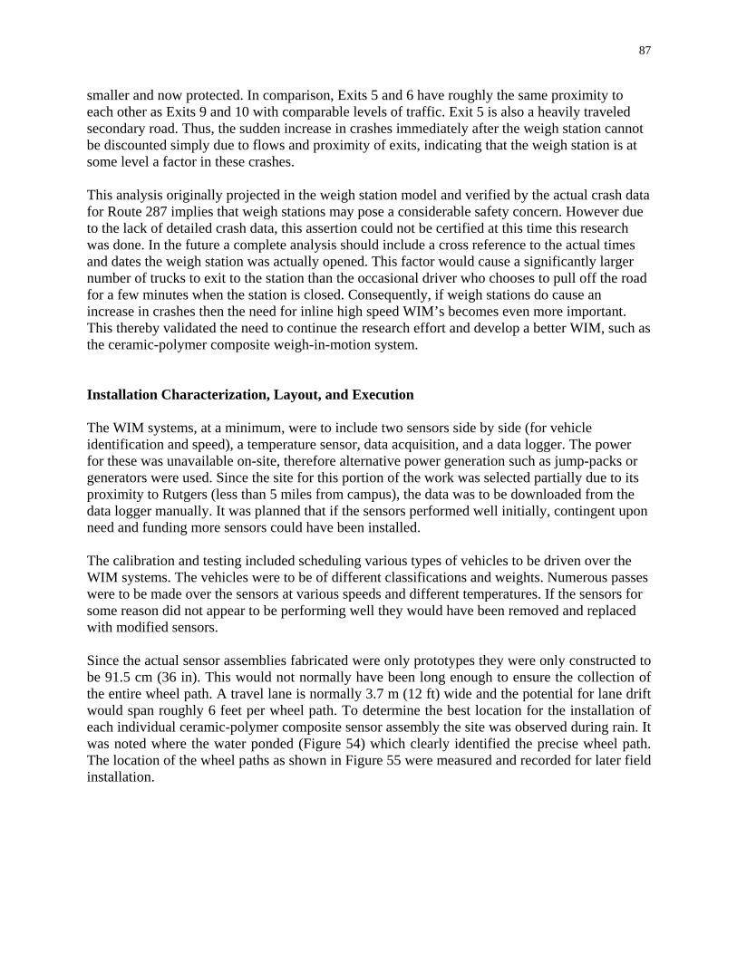
87

smaller and now protected. In comparison, Exits 5 and 6 have roughly the same proximity to each other as Exits 9 and 10 with comparable levels of traffic. Exit 5 is also a heavily traveled secondary road. Thus, the sudden increase in crashes immediately after the weigh station cannot be discounted simply due to flows and proximity of exits, indicating that the weigh station is at some level a factor in these crashes. This analysis originally projected in the weigh station model and verified by the actual crash data for Route 287 implies that weigh stations may pose a considerable safety concern. However due to the lack of detailed crash data, this assertion could not be certified at this time this research was done. In the future a complete analysis should include a cross reference to the actual times and dates the weigh station was actually opened. This factor would cause a significantly larger number of trucks to exit to the station than the occasional driver who chooses to pull off the road for a few minutes when the station is closed. Consequently, if weigh stations do cause an increase in crashes then the need for inline high speed WIM’s becomes even more important. This thereby validated the need to continue the research effort and develop a better WIM, such as the ceramic-polymer composite weigh-in-motion system. Installation Characterization, Layout, and Execution The WIM systems, at a minimum, were to include two sensors side by side (for vehicle identification and speed), a temperature sensor, data acquisition, and a data logger. The power for these was unavailable on-site, therefore alternative power generation such as jump-packs or generators were used. Since the site for this portion of the work was selected partially due to its proximity to Rutgers (less than 5 miles from campus), the data was to be downloaded from the data logger manually. It was planned that if the sensors performed well initially, contingent upon need and funding more sensors could have been installed. The calibration and testing included scheduling various types of vehicles to be driven over the WIM systems. The vehicles were to be of different classifications and weights. Numerous passes were to be made over the sensors at various speeds and different temperatures. If the sensors for some reason did not appear to be performing well they would have been removed and replaced with modified sensors. Since the actual sensor assemblies fabricated were only prototypes they were only constructed to be 91.5 cm (36 in). This would not normally have been long enough to ensure the collection of the entire wheel path. A travel lane is normally 3.7 m (12 ft) wide and the potential for lane drift would span roughly 6 feet per wheel path. To determine the best location for the installation of each individual ceramic-polymer composite sensor assembly the site was observed during rain. It was noted where the water ponded (Figure 54) which clearly identified the precise wheel path. The location of the wheel paths as shown in Figure 55 were measured and recorded for later field installation.

88

Figure 54 Field observation of water ponding in the wheel paths.

Figure 55 Final proposed location for the installation of the sensor assemblies.

The install was performed over two (2) days with four (4) workers, with the installation being completed on October 16th. The first day was sunny, 29.4oC (85oF). A mock run of the installation was performed in the laboratory as shown in Figure 56 the prior evening to ensure that all materials and equipment necessary would be brought to the field. All sensors, equipment, tools, and materials were loaded in the University box truck and brought to the site.

89

Figure 56 Photograph of ceramic-polymer composite sensor assembly and chairs laid-out

in the laboratory.

Once on site, safety gear and traffic control was the first priority. All installation personnel wore safety vests and hard hats. Traffic cones were placed to close the station, protect personnel, and deter traffic flow from the station ramp. The box truck was also used to protect the workers from the oncoming traffic. After traffic control was established, the position of the each sensor was marked out with spray paint, as shown in Figure 57, according to a layout plan that had been previously prepared. The blade on the saw was then adjusted in order to achieve the desired cutting depth. It was found that one person, who would guide the saw by holding both the back and front handles as shown in Figure 58, could best operate the saw. This was necessary for controlling the saw along the exact cutting path. This procedure came about through trial and error as initial attempts of controlling the saws cutting line and depth were a problem due to difficulty in communicating between two operators or an operator and a navigator.

Figure 57 Photograph of the site layout for the installation of the sensors.

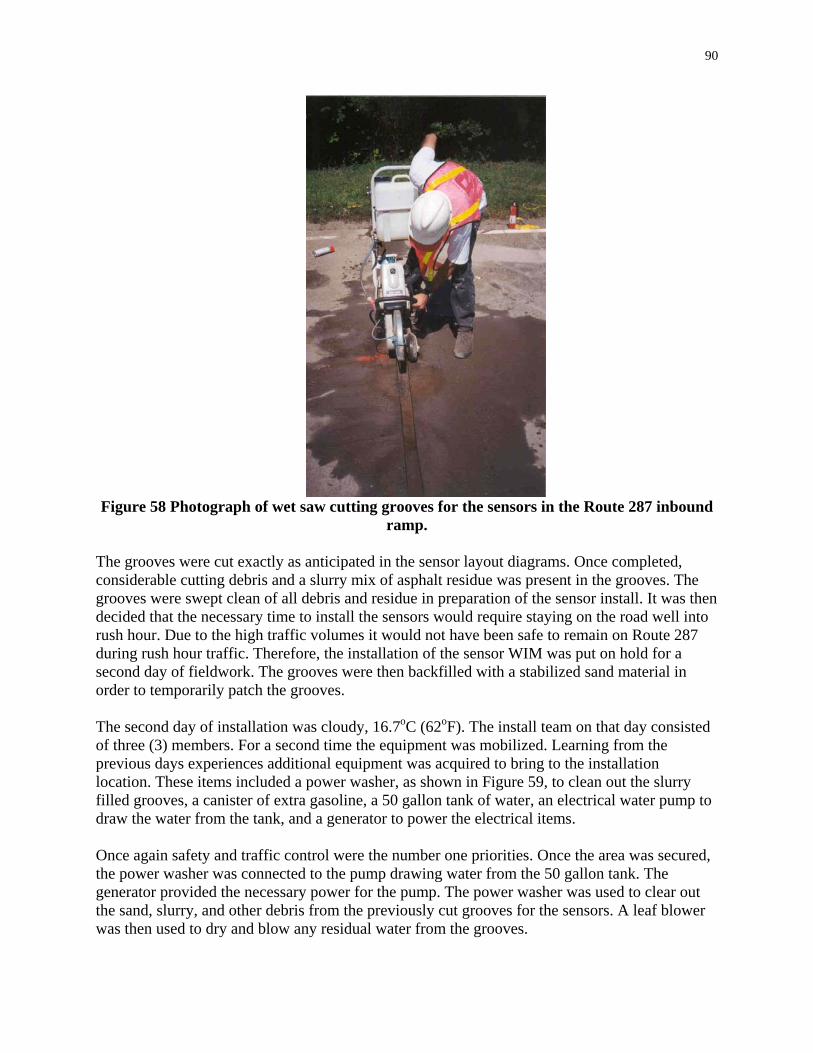
90

Figure 58 Photograph of wet saw cutting grooves for the sensors in the Route 287 inbound

ramp.

The grooves were cut exactly as anticipated in the sensor layout diagrams. Once completed, considerable cutting debris and a slurry mix of asphalt residue was present in the grooves. The grooves were swept clean of all debris and residue in preparation of the sensor install. It was then decided that the necessary time to install the sensors would require staying on the road well into rush hour. Due to the high traffic volumes it would not have been safe to remain on Route 287 during rush hour traffic. Therefore, the installation of the sensor WIM was put on hold for a second day of fieldwork. The grooves were then backfilled with a stabilized sand material in order to temporarily patch the grooves. The second day of installation was cloudy, 16.7oC (62oF). The install team on that day consisted of three (3) members. For a second time the equipment was mobilized. Learning from the previous days experiences additional equipment was acquired to bring to the installation location. These items included a power washer, as shown in Figure 59, to clean out the slurry filled grooves, a canister of extra gasoline, a 50 gallon tank of water, an electrical water pump to draw the water from the tank, and a generator to power the electrical items. Once again safety and traffic control were the number one priorities. Once the area was secured, the power washer was connected to the pump drawing water from the 50 gallon tank. The generator provided the necessary power for the pump. The power washer was used to clear out the sand, slurry, and other debris from the previously cut grooves for the sensors. A leaf blower was then used to dry and blow any residual water from the grooves.

91

Figure 59 Photograph showing the power washing and blowing of the groove to remove

debris and water.

The ceramic-polymer sensor assembly’s wires were then fished through a plastic conduit, which was to be placed in the ground. This was done twice, thus two conduits, one for each sensor assembly. The thermocouple was also fished through a third plastic conduit. Trenches for the conduit and a hole for the control/junction box were then excavated by hand. The dimensions of the trenches, as shown in Figure 60, were 20 cm (8 in) in depth, 15 cm (6 in) in width, and about 3.7 m (12 ft) in length. Each trench originated at the edge of the pavement and converged, at roughly a forty-five degree angle, at the control/junction box.

Figure 60 Photograph of the groove with the wires and plastic conduit ready for epoxy

infiltration.

92

Spacers/chairs were placed in the grooves to level and support the ceramic-polymer sensor assembly. Once placed, the sensor assembly was positioned at a height where the top surface was just below the roadway grade as shown in Figure 61. The entire groove was then outlined by duct tape as to create a slight raised lip, thus when removed the cured epoxy will extend just above the roadway grade. The raised lip is a common installation practice and was desired in order to ensure activation of the sensor. Once the sensor assemblies were completely prepared the wire-filled-conduits were then placed in the trenches. The plastic conduit extended roughly 10 cm (4 in) into the open groove at the edge of the pavement. This was done in order to protect the interface, achieve good bonding, and ensure a watertight seal at the entrance to the conduit.

Figure 61 Photograph of ceramic-polymer composite sensor assembly being placed in

groove at the Route 287 weigh station.

The PU-200 epoxy was then prepared by mixing the two agents as recommended. Mixing was performed for a minimum of 3 minutes with an electric drill equipped with a mixing blade commercially used for plaster. The sensor assemblies were then temporarily removed from the grooves, as shown in Figure 62, to allow the epoxy to completely infiltrate all cavities under the sensor. The epoxy was placed in the groove up to the level of the support chairs, at which time the sensor assembly was then repositioned onto the first layer of the epoxy and chairs. The epoxy is self-leveling and flowed into and around the groove, however this process ensured that the epoxy completely infiltrated the area below the sensor assembly. Following the insertion of the sensor assembly back into the groove the remaining cavity was then completely filled with epoxy. The epoxy was allowed to flow over and around the sensor assembly ensuring enough cover on all sides, thus fully encapsulating the assembly.

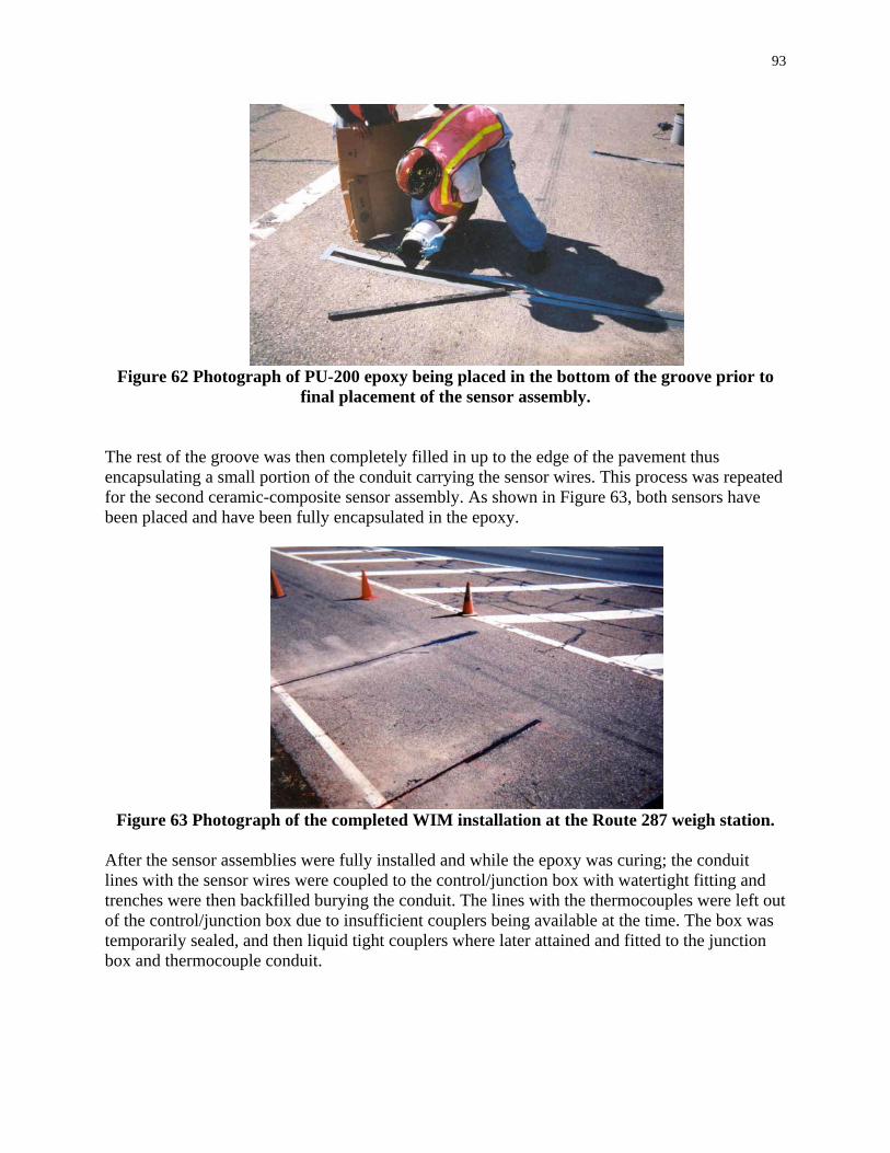
93

Figure 62 Photograph of PU-200 epoxy being placed in the bottom of the groove prior to

final placement of the sensor assembly.

The rest of the groove was then completely filled in up to the edge of the pavement thus encapsulating a small portion of the conduit carrying the sensor wires. This process was repeated for the second ceramic-composite sensor assembly. As shown in Figure 63, both sensors have been placed and have been fully encapsulated in the epoxy.

Figure 63 Photograph of the completed WIM installation at the Route 287 weigh station.

After the sensor assemblies were fully installed and while the epoxy was curing; the conduit lines with the sensor wires were coupled to the control/junction box with watertight fitting and trenches were then backfilled burying the conduit. The lines with the thermocouples were left out of the control/junction box due to insufficient couplers being available at the time. The box was temporarily sealed, and then liquid tight couplers where later attained and fitted to the junction box and thermocouple conduit.

94

Figure 64 Photograph of control/junction box linked to sensor wires and ready to be

buried.

During the epoxy gel time, about half an hour after mixing, the duct tape was removed from the perimeter of the groove and epoxy was allowed to fully cure. The area with the newly installed sensors remained closed for another one and a half hours to ensure that the epoxy had fully cured and was hard enough to be opened to vehicle traffic. Field Testing of Ceramic-Polymer Composite Sensor Assemblies After installation, the ceramic-polymer sensor assemblies were field tested. Various vehicles of known weight were to be driven over the sensor assemblies and corresponding voltages measured. The data was to be analyzed and evaluated to determine how the sensor assemblies performed. Initial Testing Results (Immediately After Sensor Installation) Once again, as in the initial limited field trial in the parking lot the Rutgers SPA van was used. The van’s individual tire loads were once again measured and found to have remained relatively unchanged. Each of the front tires and back tires were found to weigh (i.e. carry a load of) 690 kg (1,521 lbs) and 783 kg (1,727 lbs) respectively. The van was then driven over the sensor assemblies and data collected. As this was real world field conditions, as the testing was conducted on Rt. 287, there was a high degree of variability in the speed and manner in which the van passed over the sensor. In some cases the deceleration started early and caused a spike on the first axle. In other cases there was acceleration still occurring when the van passed over the sensor resulting in a spike on the second axle. Speed was also highly variable due to safety concerns and the flow of surrounding traffic. A sample of the data that was collected can be seen in Figure 65, this result is extremely close to the results obtained much earlier in this research effort with the prototype sensor during the limited field trial in the parking lot. In the original case, the voltage was roughly 0.1V versus

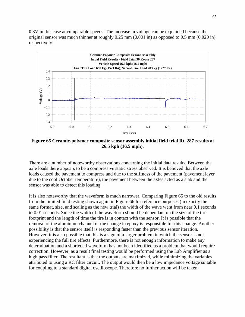
95

0.3V in this case at comparable speeds. The increase in voltage can be explained because the original sensor was much thinner at roughly 0.25 mm (0.001 in) as opposed to 0.5 mm (0.020 in) respectively.

Ceramic-Polymer Composite Sensor Assembly Initial Field Results - Field Trial 30 Route 287

Vehicle Speed 26.5 kph (16.5 mph)First Tire Load 690 kg (1521 lbs); Second Tire Load 783 kg (1727 lbs)

-0.3

-0.2

-0.1

0

0.1

0.2

0.3

0.4

5.9 6.0 6.1 6.2 6.3 6.4 6.5 6.6 6.7

Time (sec)

Vol

tage

(V)

Figure 65 Ceramic-polymer composite sensor assembly initial field trial Rt. 287 results at

26.5 kph (16.5 mph).

There are a number of noteworthy observations concerning the initial data results. Between the axle loads there appears to be a compressive static stress observed. It is believed that the axle loads caused the pavement to compress and due to the stiffness of the pavement (pavement layer due to the cool October temperature), the pavement between the axles acted as a slab and the sensor was able to detect this loading. It is also noteworthy that the waveform is much narrower. Comparing Figure 65 to the old results from the limited field testing shown again in Figure 66 for reference purposes (in exactly the same format, size, and scaling as the new trial) the width of the wave went from near 0.1 seconds to 0.01 seconds. Since the width of the waveform should be dependant on the size of the tire footprint and the length of time the tire is in contact with the sensor. It is possible that the removal of the aluminum channel or the change in epoxy is responsible for this change. Another possibility is that the sensor itself is responding faster than the previous sensor iteration. However, it is also possible that this is a sign of a larger problem in which the sensor is not experiencing the full tire effects. Furthermore, there is not enough information to make any determination and a shortened waveform has not been identified as a problem that would require correction. However, as a result final testing would be performed using the Lab Amplifier as a high pass filter. The resultant is that the outputs are maximized, while minimizing the variables attributed to using a RC filter circuit. The output would then be a low impedance voltage suitable for coupling to a standard digital oscilloscope. Therefore no further action will be taken.

96

PZT Composite Sensor Parking Lot Test 23 Vehicle Speed 32kph (20mph)

First Tire Load 690 kg (1521 lbs); Second Tire Load 783 kg (1727 lbs)

-0.3

-0.2

-0.1

0

0.1

0.2

0.3

0.4

0.4 0.5 0.6 0.7 0.8 0.9 1 1.1 1.2

Time (sec)

Vol

tage

(V)

Figure 66 Ceramic-polymer composite sensor assembly limited field trial limited field trial

testing at 32kph (20 mph).

The initial testing was performed in October and the results were exceedingly good. Since the initial results were extremely positive, and in the laboratory testing phases there was an apparent break-in period it was decided to leave the sensor in-place for a period of time and then perform a complete battery of tests using numerous known weight vehicles. In addition, with the winter months quickly approaching and the field setup required to collect data it was decided to evaluate the performance after the winter season in the spring. Testing Results Seven Months Later (Post Winter Season) The following section provides several sample plots of the data collected using the same procedure as the initial testing from when the sensor was installed. As can be seen in Figure 67, Figure 68, Figure 69, and Figure 70 there was a significant performance drop from the initial installation.

97

Ceramic-Polymer Composite Sensor Assembly Field Trial 21 Route 287 Vehicle Speed 19 kph (12 mph)


-0.25-0.2

-0.15

-0.1-0.05

00.05

0.1

0.150.2

0.25

1.0 1.1 1.2 1.3 1.4 1.5 1.6 1.7 1.8

Time (sec)

Vol

tage

(V)

Figure 67 Ceramic-polymer composite sensor assembly field trial Rt. 287 results after

winter season at 19 kph (12 mph).



-0.25-0.2

-0.15-0.1

-0.050

0.050.1

0.150.2

0.25

2.0 2.1 2.2 2.3 2.4 2.5 2.6 2.7 2.8

Time (sec)

Vol

tage

(V)


winter season at 21 kph (13 mph).

98

Ceramic-Polymer Composite Sensor Assembly Field Trial 25 Route 287 Vehicle Speed 22.5 kph (14 mph)


-0.25-0.2

-0.15-0.1

-0.050

0.050.1

0.150.2

0.25

2.6 2.7 2.8 2.9 3.0 3.1 3.2 3.3 3.4

Time (sec)

Vol

tage

(V)


winter season at 22.5 kph (14 mph).



-0.25-0.2

-0.15-0.1

-0.050

0.050.1

0.150.2

0.25

1.9 2.0 2.1 2.2 2.3 2.4 2.5 2.6 2.7

Time (sec)

Vol

tage

(V)


winter season at 29 kph (18 mph). The sensor assemblies still functioned but the output voltages are diminished by 66% to 83% of that of the original voltage output. Similar residual stress patterns are other trends that were still observed but for all intents the sensor assemblies were considered failed. During fabrication it was thought that a ‘parallel’ fabrication process should be used instead of a ‘series’. Therefore, instead of the copper sheets collecting the full voltage and relaying it via one set of lead wires back to the data acquisition unit; every two sensors were grouped together in series and connected via lead wires back to the computer. Therefore, the sensor was fabricated

99

with 12 individual active sensors and there are 6 sensor groups, each group making up 15.24cm (6 in) lengths. It was thought that this would prove useful for field diagnostics if such a failure occurred. A multi-meter was connected to each terminal and capacitance measured, the results of which can be seen in Table 30. From the table it can be determined that sensor group 2 and 4 (sensors three, four, seven, and eight or any combination therein) have a failure and are not collecting nor relaying the voltages properly to the data acquisition computer. Unfortunately, with so many sensor segments showing problems it is not possible to by pass the set of bad sensor and continue collecting data. It is possible that the active sensor material itself is still intact but that cannot be determined without removing, dissecting the sensor, and analyzing each component. It was therefore determined that once the field testing was complete the sensor should be removed from the roadway for a full forensic analysis.

Table 30 Table summarizing capacitance of sensor segments by group.

Sensor Segments Capacitance (pF) i.e. 10-6

One and Two 160

Three and Four 35

Five and Six 400

Seven and Eight 14

Nine and Ten 400

Eleven and Twelve 200

100

Tractor Trailer Addendum to Field Testing During the field evaluation of the sensor is was not uncommon for tractor trailers to enter the weigh station where the sensor was installed; the trucks were not existing to be weighed but merely using the closed station as a rest stop. Taking advantage of these additional test vehicles was a welcome addition to the data evaluation effort. Since the tractor trailers were neither planned test vehicles nor was the weight station open; vehicle speeds had to be estimated from back calculation assuming standard axle spacing however vehicle/axle weights remained as completely unknown variables. Therefore the amount of analysis that could be conducted without known weight was extremely limited; however the data available is presented below as a frame of reference for future research efforts. The speed of the trucks was unknown, however the axle spacing is fairly typical and the speed can be back calculated. The distance axles can be assumed to be roughly 2.5 m (8.2 ft), 0.6 m(2.0 ft), 3,5 m (11.5ft), and 0.6 m (2.0 ft) respectively. Back calculating from the timestamps for locations of the waveform peaks an estimated speed can be determined for each vehicle. Figure 71 is the data from a tractor trailer of unknown weight immediately after the sensor was installed; and Figure 72 is the data from a tractor trailer seven months after installation. Both vehicles were traveling at very close to the same speed but even just comparing the steering axle it can be seen that the signal is significantly degraded. As a determination was already made to remove the senor assembly from the field and conduct a complete forensic analysis, there is no need for further discussion of this data from the tractor trailers.


Vehicle Speed 72.5 kph (45 mph)Tractor Trailer - Vehicle Loading Unknown

-2

-1

0

1

2

3

4

0.80 0.85 0.90 0.95 1.00 1.05 1.10 1.15 1.20 1.25

Time (sec)

Vol

tage

(V)

Figure 71 Ceramic-polymer composite sensor assembly results of tractor trailer loading,

initial field trial Rt. 287 results at 72.5 kph (45 mph).

101



-0.2

-0.15

-0.1

-0.05

0

0.05

0.1

0.15

1.15 1.20 1.25 1.30 1.35 1.40 1.45 1.50 1.55 1.60

Time (sec)

Vol

tage

(V)

A

B

C D E

Figure 72 Ceramic-polymer composite sensor assembly field trial Rt. 287 results of tractor

trailer loading, after winter season at 67.5 kph (42 mph).



FIRST AXEL

-0.2

-0.15

-0.1

-0.05

0

0.05

0.1

0.15

1.33 1.34 1.35 1.36 1.37

Time (sec)

Vol

tage

(V)

Figure 73 First axle loading results for the ceramic-polymer composite sensor assembly field trial Rt. 287 results of tractor trailer loading, after winter season at 67.5 kph (42

mph).

102



SECOND AXEL

-0.2

-0.15

-0.1

-0.05

0

0.05

0.1

0.15

1.52 1.53 1.54 1.55 1.56

Time (sec)

Vol

tage

(V)

Figure 74 Second axle loading results for the ceramic-polymer composite sensor assembly

field trial Rt. 287 results of tractor trailer loading, after winter season at 67.5 kph (42 mph).

Figure 73 and Figure 74 are worthy of note because the general trend closely matched the strain trace other researchers have observed for tandem axles, as shown in Figure 75. For example, in a recently published NCAT report “Methodology and Calibration of Fatigue Transfer Functions for Mechanistic – Empirical Flexible Pavement Design” there are very similar observations.32 In particular looking at the tandem axle waveform it can be observed that there is a sudden horizontal microstrain decrease into the negative region directly between the axles.

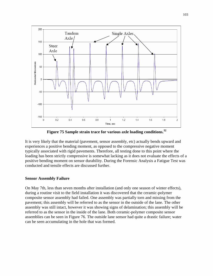
103

Figure 75 Sample strain trace for various axle loading conditions.32

It is very likely that the material (pavement, sensor assembly, etc) actually bends upward and experiences a positive bending moment, as opposed to the compressive negative moment typically associated with rigid pavements. Therefore, all testing done to this point where the loading has been strictly compressive is somewhat lacking as it does not evaluate the effects of a positive bending moment on sensor durability. During the Forensic Analysis a Fatigue Test was conducted and tensile effects are discussed further. Sensor Assembly Failure On May 7th, less than seven months after installation (and only one season of winter effects), during a routine visit to the field installation it was discovered that the ceramic-polymer composite sensor assembly had failed. One assembly was partially torn and missing from the pavement; this assembly will be referred to as the sensor in the outside of the lane. The other assembly was still intact, however it was showing signs of delamination; this assembly will be referred to as the sensor in the inside of the lane. Both ceramic-polymer composite sensor assemblies can be seen in Figure 76. The outside lane sensor had quite a drastic failure; water can be seen accumulating in the hole that was formed.

104

Figure 76 Failure of sensor assemblies; outside of lane (left) and inside of lane (right).

The ceramic-polymer composite sensor assemblies were left in the field until the roadway had dried; they were then closely examined and photographed for forensic analysis of the failure mechanism. Following the field examination, the assemblies were then removed from the roadway and brought back to the laboratory. Figure 77 shows clearly how dramatically the outside lane sensor had failed; the wires and the piezoelectric material itself of the sensor was exposed and no longer embedded in the PU-200 epoxy.

Direction of traffic flow

105

Figure 77 Close-up examination of failed outside of lane sensor assembly. The inside lane sensor as shown in Figure 78 had a pothole forming just in front of the

sensor. It was believed that if left unchecked that the mode of failure for the inside lane would have been identical to the outside lane sensor. A pothole would have formed just past the sensor and the epoxy would have been pushed forward resulting in a failure directly in the center of the wheel path. The sensor assembly would have sheared in two and a portion of the sensor would have been pulled from the asphalt pavement.

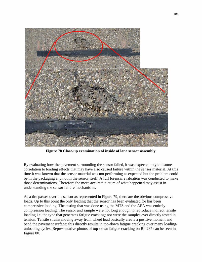
106

Figure 78 Close-up examination of inside of lane sensor assembly.

By evaluating how the pavement surrounding the sensor failed, it was expected to yield some correlation to loading effects that may have also caused failure within the sensor material. At this time it was known that the sensor material was not performing as expected but the problem could be in the packaging and not in the sensor itself. A full forensic evaluation was conducted to make those determinations. Therefore the more accurate picture of what happened may assist in understanding the sensor failure mechanisms. As a tire passes over the sensor as represented in Figure 79, there are the obvious compressive loads. Up to this point the only loading that the sensor has been evaluated for has been compressive loading. The testing that was done using the MTS and the APA was entirely compression loading. The sensor and sample were not long enough to reproduce indirect tensile loading i.e. the type that generates fatigue cracking; nor were the samples ever directly tested in tension. Tensile strains moving away from wheel load basically create a positive moment and bend the pavement surface; this directly results in top-down fatigue cracking over many loading-unloading cycles. Representative photos of top-down fatigue cracking on Rt. 287 can be seen in Figure 80.

107

Compressive Zone

Tensile Zone

Cracking Due to Tensile Effects

Pavement or WIM Sensor Surface

Tire Loading

Pavement Deflection

Stress Distribution

Figure 79 Transverse stress distribution on roadway surface due to tire loading.

Figure 80 Top-down fatigue cracking on Rt. 287.33

The load transfer mechanism is largely dependant on the rigidity of the pavement and the compressive and tensile effects are directly related. The strain effects in relationship to average month temperature can be seen in Figure 81. In the colder months the compressive loading

Negative Enhanced Image

Crack

Core Sample

108

generates its lowest strain reading which means that the WIM sensor voltage would also be lower. This directly correlates to the observed voltage output in the earlier laboratory experiments. Despite the lower WIM voltage readings the corresponding tensile loads are also minimized. This will minimize sensor and epoxy cracking as a result of the fatigue and the positive bending moment generated. Conversely, in the summer months the compressive and tensile loads are at their maximum strains, this not only maximizes the output of the WIM sensor voltage but maximizes the potential for damage. In summary, a more elastic material will result in less tensile fatigue strains and minimize the effects of top-down type tensile effects on the WIM sensor assembly. In the APA tests cracking was observed in the more rigid epoxy in the wheel path. However, in light of the indirect tensile fatigue it is even more critical to select an epoxy that has an elastic modulus in the lower range as compared to asphalt. For more information of the fatigue relationship on the sensor, please refer to the forensic analysis of tensile effects on the sensor performance section later in this dissertation.

Figure 81 Strain effects with respect to seasonal temperature variation versus distance

from center of wheel load.33

Assuming that it is accurate to say that at least a similar mechanism works longitudinally as well as transversely, then this may help explain why a pothole formed directly in front of the sensor assembly. However, this deals directly with the bow wave phenomena which is highly debated in the pavement industry. In theory pavements with higher roughness and low strength may increase the rolling resistance of the tire by creating a pavement wave directly in front of the tire. According to an NCHRP research report “One common cause of sensor failure is when sensors

-170-160-150-140-130-120-110-100-90-80-70-60-50-40-30-20-10

01020

0 5 10 15 20 25 30 35Distance from Center of Wheel Load (inches)

Hor

izon

tal M

icro

-Str

ain,

Exx

(in/

in)

Jan.

Feb.

March

April

May

June

July

Aug.

Sept.

Oct.

Nov.

Dec.

Contact Radius

109

directly experience horizontal forces from tire contact. This often leads to early fatigue failure for both sensors and the bonds between sensors and pavement.”13 This would appear to be the reason why the asphalt failed and there appears to be a high degree of correlation between the transverse tensile stresses discussed previous and the longitudinal tensile stresses. From the visual inspection it is clear that the cause of failure is both a pure delamination of the asphalt-epoxy interface as well as a general delamination of the asphalt itself. Therefore the system characterization question of packaging remains. Since the initial thermal expansion tests were done on epoxy prisms embedded in an asphalt pavement brick sample, basically a confined test, it was though that an unconfined test would yielded a more accurate picture of the compatibility of the epoxies and the asphalt. As materials were not readily available this testing was not redone, and will be recommended for future work. Recovery of Sensor Assembly The entire ceramic-polymer composite sensor assembly from the inside lane was recovered. A portion of the outside lane sensor was also recovered, pieces of that sensor were found strewn throughout the roadway. A significant portion of these pieces, many of them being chunks of PZT composite, were also recovered. The recovered sensor assemblies were removed from the roadway by hand, simply by pulling up on the epoxy; thus demonstrating how weak the bond between the sensor and the roadway had degraded to. Since the inside lane sensor assembly was recovered largely intact it can be assumed that all sensor degradation would have been as a result of the damage experienced while installed on the roadway and not during the removal process. The entire sensor as removed from the field can be seen in Figure 82.

Figure 82 Recovered sensor assembly from Rt. 287 field installation.

Conclusions Final Laboratory and Field Trials and Analysis

Based on the results of the long term durability and degradation tests of the sensor (asphalt versus concrete) effort the following can be concluded:

• The asphalt pavement sample experienced more than three (3) times the

deformation (rutting) than the concrete. As the asphalt sample continued to deform, it compacted the material below the sensor and therefore acted more like the very

110

rigid concrete sample, by the end of the 100,000 cycles the two outputs were nearly indistinguishable.

• For the asphalt pavement sample, 15.6% of the overall 16.5% (95% of the total reduction) voltage drop occurs within the first 10,000 cycles followed by a fairly flat output (approximately 5% further deterioration) for the reaming 90,000 cycles. It is likely that the deformation of the asphalt surrounding the sensor created an initial amplification of sensor deterioration, and thus the eventual damage the sensor would experience occurred very early on in the experiment.

• The concrete sample did not experience significant rutting, and therefore the sensor deterioration occurred over a much longer period of time. For the concrete sample, a 95% reduction is not measured until the sample reaches the 20,000 to 40,000 range.

• This is not to imply that the sensor installed in concrete failed earlier, or that the sensor in concrete was better; both samples experience nearly identical output between 60,000 to 100,000 cycles. It is believed that the sensor will undergo an initial ‘break-in’ period where the sensor will undergo some deterioration. This may explain why commercially available sensors require such frequent recalibration when installed in real field conditions.

• There is a widely held belief that WIM’s installed in concrete will perform better because the visco-elastic asphalt variability is removed among other reasons, however by comparing the asphalt and the concrete samples for the same sample sets it clearly shows that the asphalt sample has a much lower standard deviation earlier.

Based on the results of the field testing of the ceramic-composite sensor assemblies’ effort the following can be concluded:

• The initial testing results were satisfactory, for the same weight and temperature as

the initial limited field trial testing conducted in a parking lot, these results yielded voltages that were roughly in the range of 0.3V versus 0.1V in the original testing.

• After seven months the sensor assemblies still functioned but the output voltages were diminished by 66% to 83% of that of the original voltage output. Similar residual stress patterns and other trends were still observed, but for all intents the sensor assemblies were considered failed.

• From the visual inspection it was clear that the cause of packaging failure is both a pure delamination of the asphalt-epoxy interface as well as a general delamination of the asphalt itself. Therefore the system characterization question of packaging remains.

111

CONCLUSIONS AND FUTURE RESEARCH WORK The goal of this research effort was to develop a sensor with a higher level of accuracy than can be attained by available WIM systems under actual field conditions. A recent NCHRP Study Synthesis 386, published in 2008, conducted a nationwide survey of all 50 States, DC, and Puerto Rico. One of the survey questions was “In your opinion, what are the most urgent WIM technical needs at present and what studies need to be conducted to address them?” A summary of relevant comments from the respondents is provided in Table 2. However in general, respondents wanted more accurate, more durable, and less temperature dependant sensors as well as better epoxies/grouts to ensure installations last longer. Some of the comments were “better, more reliable sensors. Better epoxy,” “making the BL piezos last longer regardless of what kind of traffic,” “BL piezos are temperature and speed sensitive,” “develop more accurate sensors,” “Better grouts for piezos,” “type II WIM perspective sensors are still the weak link,” and finally to summarize the general consensus of the survey “sensors and installation methods that last.”6 This research effort focused specifically on these issues, and thus this recent survey validates the national need the work performed. Piezoelectric ceramic-polymer composite sensor assemblies were fabricated for use as WIM sensors for measuring large loads. A complete review of the system characterization was conducted; which evaluated the active sensor themselves and the packaging and epoxy used to embed them in the roadway. Once the system characterization effort was complete, the ceramic-polymer composite sensor assemblies were installed on a full-scale highway Rt. 287 test scenario in order to perform actual measurements. The output was evaluated and a forensic review of the material was conducted to determine potential issues and develop future criteria to be further researched. Conclusions from Previous Research

Based on the results of the initial sensor fabrication effort as reported in the Implementation of Advanced Fiber Optic and Piezoelectric Sensor – Fabrication and Laboratory Testing of Piezoelectric Ceramic-Polymer Composite Sensors for Weigh-in-Motion Systems” FHWA-NJ-1999-029 also written by the author of this report, the following can be concluded:

• It was shown that for PVDF polymer sensors versus the ceramic-polymer

composite sensor, under the same loading conditions, that the average loading output of the composite sensor is about three times that of the PVDF sensor.

• The ceramic-polymer composite sensor has superior electrical properties than that of the PVDF, including a higher d33 and thickness-coupling coefficient. The signal to noise ratio is also much better for a ceramic-polymer composite sensor and hence will detect much lower load differences with a greater accuracy.

• For a piezoelectric material, when the temperature approaches the Curie temperature (Tc) where the aligned electric dipoles are easier to rotate under heaving loading the material will depole; i.e. hence a degradation in the sensor performance. The PVDF has a Tc of only 100oC (212oF) it could easily start losing part of its piezoelectric properties at high loads at temperatures as low as 55-65oC

112

(131-149oF). To avoid thermal depolarization a “safe operating temperature would normally be about half way between 0oC and the Curie point”34 For the PVDF materials this implies that that use above 60oC (140oF) is not recommended. This limit 60oC (140oF) is dangerously close to the upper thermal limit of 64oC (147oF) in summer within a 98% reliability35 as per FHWA that HMA experiences in New Jersey. However, the ceramic-polymer composite sensor is more rugged with a much higher Tc of ~190oC (374oF).

• The laboratory results from the initial prototype, voltage output with respect to loading and temperature proved to reliably yield the same results or at least the same trends.

Conclusions Conclusions are summarized at the end of each phase of work, however, key elements of the conclusions are as follows:

1) Development and Evaluation of the Sensor • The simulation model showed a clear advantage of using a WIM to increase the

efficiency of a static scale operation. • The more accurate a WIM, the more efficient the weigh station will become. • At higher volumes, by using a WIM with an accuracy of 10%, the FHWA standard

configuration catches 70-80% of all violators. However, using the same configuration with an advanced WIM sensor of 5% accuracy this model can catch upward of 95% of all the violators. This reduced the amount of vehicles being weighed statically and reduced queue lengths.

• There is one potential drawback to a more accurate WIM sensor. While modeling the advanced WIM sensor (i.e. 5% accuracy), there was a significant correlation between the increased accuracy and hard decelerations; hard decelerations are an indication of vehicle crashes. The weigh station model still requires the trucks to move to an isolated lane or a bypass road, therefore the trucks are still required to maneuver through traffic, changing lanes, etc. It is believed that since the pre-screening was so efficient in detecting overweight vehicles as traffic levels increase the queue length never gets long enough to close the scale. Therefore, 100% of trucks will be either pre-screened or required to exit the roadway to the static scale. The exiting and entering of trucks on the roadway as well as the associated lane shifting is conducive to creating an environment where more crashes may occur.

2) System Characterization -Advanced Prototype Development (Packaging and Epoxy Selection) • Based on the APA rutting evaluation no epoxy can be determined as clearly

superior. Ranking was done considering the following priorities: 1) did not have actual epoxy cracking (longitudinal cracking); 2) nor demonstrated rigidity (significant protrusion from the sample surface; 3) nor flash point concerns; 4) nor long wait times until traffic ready;

113

PU-200 appeared to be the best compromise based on the APA rut testing, with no catastrophic failure nor significant material or handling concerns that had the least measured delamination. However this does not mean that PU-200 truly outperformed the other epoxies.

3) Final Laboratory and Field Trials and Analysis • There is a widely held belief that WIM’s installed in concrete will perform better

because the visco-elastic asphalt pavement variability is removed among other reasons, however by comparing the asphalt and the concrete pavement samples for the same sample sets it clearly shows that the asphalt sample has a much lower standard deviation earlier.

• After seven months the sensor assemblies still functioned but the output voltages were diminished by 66% to 83% of that of the original voltage output. Similar residual stress patterns and other trends were still observed but for all intents the sensor assemblies were considered failed.

Summary Recommendations for Future Research In summary, the ceramic-polymer composite sensors performed extremely well in all laboratory testing. However, under full-scale field implementation, a rather aggressive goal, the sensors and sensor assemblies experienced some level of failure. It is believed that there would have been a better overall performance if:

• Concerning the electroding, it is thought that a pre-encapsulation in a rigid elastomeric block may help to ensure the electroding remains affixed to the active material. In addition, the roadway epoxy is somewhat permeable (PU-200 has a water absorption rate of 2.5% as per the manufacturer) therefore if the active material is encased in an impermeable block the electrode as well as the sensor will be impervious to roadway salts and acids.

• The APA rut testing was extremely useful in selecting an epoxy for use. However, there is still much that is not known about how the epoxy interfaces with the roadway and the differences between a pure delamination and a delamination due to asphalt debonding. It is recommended to install a series of epoxies on a highway and observe the outcome without maintenance. All the epoxies (lets say five installations of each) could be installed on the roadway so they experience identical loading and then monitored for a period of time. Core samples could be taken of the pavement to verify material properties of the surrounding roadway. In addition non destructive testing such as GPR could be conducted on the segments to determine if there are any measureable pre-indicators of failure and maybe gain some insight into the exact failure mechanisms.

• Finally, once the above items are addressed a new full-scale field implementation could be conducted to re-evaluate the ceramic-polymer composite sensor assemblies. The field installation must be performed in a good quality pavement with significant remaining useful life; it is strongly believed that one of the primary reasons why the Rt. 287 full scale field installation failed was simply due to poor pavements that have fatigued well beyond their useful life.

114

REFERENCE 1 C. E. Lee, ASTM Standardization News, 19, 32, (1991) 2 F. Roberts, P. Kandhal, E. Brown, D. Lee, T. Kennedy, Hot Mix Asphalt Materials, Mixture Design and Construction, (NAPA Research and Education Foundation, Lanham, MD, 1994), p. 416 3 Trigg Industries International, Brass Linguini Product Description Sheet 4 Product Data Sheet, RoadtraxTM series P and TP piezoelectric polymer traffic sensor, Number 29, Atochem Sensors Inc., Piezo film sensor division, Valley Forge PA 5 Whitely, Lou and Vitillo, Nicholas, New Jersey Department of Transportation memo December 1999 6 A. T. Papagiannakis, R. Quinly, and S.R. Brandt, “Highway Speed Weigh-In-Motion Ststem Calibration Practices” NCHRP 386 2008 7 Website, http://www.physikinstrumente.com/tutorial/4_15.html, 2/7/2006 8 Website, http://www.physikinstrumente.com\PI Piezo Tutorial Fundamentals of Piezoelectricity and Piezo Actuators.htm as of 2/7/2006 9 A. Safari, J. Physics III France, 4, 1129 (1994) 10 G. Bailleul, in National Traffic Data Acquisition Conference, vol 2, p. 596, (1996) 11 X. Zhi, A. Shalaby, D. Middleton, and A Clayton “Evaluation of weigh-in-motion in Manitoba” Canadian Journal of Civil Engineering, v26 n5 1999 p 655 -666 12 C. Lee “Standards for highway Weigh-in-motion (WIM) systems” ASTM Standardization New v19 n2 Feb 1991 p 32-37 13 Mark Hallenbeck & Herbert Weinblatt, “ Equipment for Collecting Traffic Load Data”, NCHRP Report 509 2004 14 J. Victor Chatigny and Lester E. Robb, Piezo Film Sensors Pennwalt Corporation, Piezo Film Sensors Magazine, March 1999 15 FHWA – DP 90 Asphalt Mix Design and Field Management Database, 1997 16 ASTM E1318, ASTM committee 17 on Pavement Management Technologies, 1993 17 Glassco, Richard A., “Simulation of ITS Benefits at a Truck Weigh Station” Mitretek Systems 18 Harvey, Bruce A. and Mussa, Renatus Improving Operation of FDOT Telemetered Traffic Monitoring Sites, 2003, Florida Department of Transportation BC-596 19 PU-200 Data Sheet and Material Safety Data Sheet Global Resins Corsham, Wiltshire, England 20 E-Bond G-100 Safety Data Sheet E-Bond Epoxies Inc., Fort Lauderdale, FL 21 ECM P5G/P6G Resins Safety Data Sheet, Electronique Control Mesure Inc. 22 AS 475 Material Safety Data Sheet Degussa Corporation Edmonton, Alberta, Canada 23 E-Bond1261 Technical Data Sheet and Material Safety Data Sheet E-Bond Epoxies Inc., Fort Lauderdale, FL 24 Dural 306 Technical Data Sheet and Material Safety Data Sheet, Tamms Industries Kirkland, Illinois 25 Dural 340 Technical Data Sheet and Material Safety Data Sheet, Tamms Industries Kirkland, Illinois 8/99 26 Bondo 7084 Piezo/Traffic Sensor Sealant, Bondo/Mar-Hyde Corporation Atlanta Georgia 27 Website for MM 80 Spec Data, http://www.metzgermcguire.com/mm80spec.htm, 10/18/00 28 Dural 335 Technical Data Sheet and Material Safety Data Sheet, Tamms Industries Kirkland, Illinois 12/98

115

29 AASHTO T-283 “Resistance of Compacted Bituminous Mixture to Moisture-Induced Damage” 30 Website, http://training.ce.washington.edu/WSDOT/Modules/05_mix_design/05-6_body.htm as of February 2009 31 Website, http://training.ce.washington.edu/WSDOT/Modules/05_mix_design/05-6_body.htm as of February 2009 32 A. Priest, D. Timm, Methodology and Calibration of Fatigue Transfer Functions for Mechanistic – Empirical Flexible Pavement Design. Kimley-Horn and Associates, Inc. National Center for Asphalt Technology Auburn University, Alabama, December 2006 33 T. Bennert, Evaluation of Poisson’s Ratio, RAPL September 2004 34 J. Victor Chatigny and Lester E. Robb, Piezo Film Sensors Pennwalt Corporation, Piezo Film Sensors Magazine, March 1999 35 FHWA – DP 90 Asphalt Mix Design and Field Management Database, 1997

Implementation of Weigh-in-Motion (WIM) Systems · that good data can be useful for bridge...

Documents

Transcript of Implementation of Weigh-in-Motion (WIM) Systems · that good data can be useful for bridge...