Implementation of a visual difference metricusing commodity graphics hardware

Jered E. Windsheimer, Gary W. Meyer

Department of Computer Science and Engineering, University of Minnesota200 Union Street SE, Minneapolis, MN 55455

ABSTRACT

A visual difference metric was implemented on a commodity graphics card to take advantage of the increasedprocessing power available today in a Graphics Processing Unit (GPU). The specific algorithm employed was theSarnoff Visual Discrimination Metric (Sarnoff VDM). To begin the implementation, the typical architecture ofa contemporary GPU was analyzed and some general strategies were developed for performing image processingtasks on GPUs. The stages of the Sarnoff VDM were then mapped onto the hardware and the implementationwas completed. A performance analysis showed that the algorithm’s speed had been increased by an order ofmagnitude over the original version that only ran on a CPU. The same analysis showed that the energy stagewas the most expensive in terms of both program size and processing time. An interactive version of the SarnoffVDM was developed and some ideas for additional applications of GPU based visual difference metrics weresuggested.

Keywords: Graphics Hardware, Graphics Processing Unit, Vision Model, Visual Difference Metric

1. INTRODUCTION

Recent improvements in Graphics Processing Units (GPUs) make it possible to execute complex image-processingtasks on commodity video cards. The vertex and pixel pipelines of modern GPUs are reprogrammable usinghigh-level programming languages to accomplish almost any task a CPU can perform. Additionally, GPUs aredesigned to execute vector and matrix operations at high speeds with high parallelism. GPUs now support fullfloating-point precision in each color channel, allowing techniques that require such precision to be more easilysupported than in the past.

There have been a number of recent attempts to exploit the increased computational power of the GPUand to use these devices in ways that they were not originally intended. Some of this work has attempted toaccomplish a specific simulation, such as ray-tracing1, 2 or cloud formation,3 on the GPU instead of the CPU.Other researchers have tried to develop general algorithms for the GPU that could be used to solve a numberof different problems. These advancements have included multi-grid simulation techniques,4 linear algebraoperators,5 and numerical solutions to least squares problems.6

In this paper we present another novel GPU application by describing a GPU based implementation of theSarnoff Visual Discrimination Model (Sarnoff VDM). A visual difference metric is a program that accepts twoversions of the same image, one a reference picture and the other a version containing artifacts, and outputs avisual difference map that indicates the places where the defects in the imperfect input image are perceptuallysignificant. There have been a number of visual discrimination metrics proposed, including some that handlecolor and motion. We have selected an early monochrome version of the Sarnoff VDM for this initial GPUimplementation.7

The remainder of the paper begins with an overview of the architecture of a modern GPU and the problemsinvolved in performing image processing tasks on a GPU. Next some of the specific implementation issues raisedby each stage of the Sarnoff VDM are addressed. Finally the resulting GPU based visual difference metric isanalyzed in terms of both instruction count and processing speed.

Further author information:J.E.W.: E-mail: windshei@cs.umn.eduG.W.M.: E-mail: meyer@cs.umn.edu

2. IMAGE PROCESSING ON THE GRAPHICS PROCESSING UNIT

The capabilities of Graphics Processing Units (GPUs) have significantly improved over the last few generations.These new capabilities allow the GPU to be treated more like a CPU. It is now possible to develop softwarewhich delegates some computationally expensive but highly parallelizable tasks to the GPU. The Sarnoff VDMis an excellent example of the sort of software that can benefit from the newest GPU features. This sectionreviews the GPU features that make implementing complex software possible, describes some issues involved indeveloping software for the GPU, and further analyzes the specifics of the Sarnoff VDM implementation.

2.1. GPU Capabilities

Early GPUs were much simpler than the current generation. The functionality of the early GPUs was fixed,and fairly limited. The hardware could perform basic geometry rasterization and texture mapping from texturesstored in local memory. Over time, the hardware improved in both speed (partially from multiple processingpipelines) and functionality, adding capabilities such as the application of multiple textures in a single pass,evaluation of 3D transformations and lighting equations, and special hardware for a small amount of pipelineprogrammability (register combiners). These improvements, and a few others that are very recent, allow muchmore to be done with the GPU than ever before.

The programmability of the GPU is undoubtedly the most significant advancement in GPU technology.The GPU no longer applies a fixed-function pipeline to each vertex and pixel it processes. Register combinerspreviously allowed a small amount of programmability, but the major portions of the pipeline were still fixed.Instead, certain stages of the rendering pipeline have been replaced with stages that apply small user-definedfunctions to the data. The programs, known as vertex programs and pixel (or fragment) programs, can bedeveloped in a high-level language (such as NVIDIA’s Cg,8 Microsoft’s HLSL or OpenGL’s glslang) and compiledto the native instruction set of the GPU. With this programmability, one can perform complex processing taskson the vertices and fragments that come down the pipeline.

A major factor in the high speed of modern GPUs is parallelism. Multiple pipelines exist for pixel process-ing, allowing different pixels of the output image to be processed at the same time. The GPU handles thistransparently, allowing the vertices and fragments being processed to easily share resources such as textures.

GPUs now allow the rendering output to be sent directly to on-card texture memory instead of the framebuffer. This feature allows the use of special rendering targets that are in formats the frame buffer doesn’tnormally support.

The GPU is fully capable of performing computations using floating-point values with high precision, but whenall output is sent to the frame buffer, much of the accuracy is discarded by the 8-bit integer color channels. GPUsnow allow textures in texture memory to use high-precision formats (such as 32-bit floating-point representationfor each color channel), so the precision can be retained when rendering to texture memory. Using high-precisiondata types in the pipeline and permitting the results to be output to high-precision texture memory allows theGPU to perform high-precision calculations that are necessary for many complex tasks.

One of the other critical new features is dependent texture lookup. In earlier GPU generations each fragmentwas only allowed to access textures at the coordinates specified by the pipeline, generally the texture coordinatesinterpolated from the vertices. Now a pixel program is allowed to access any pixel of its associated textures,at any time the program wishes. This feature lets one treat texture maps much like two-dimensional arrays innormal software. Textures can be used as lookup tables containing approximations to complex functions, or apixel program can read the texels around its usual texture coordinate, allowing arbitrary filtering to take place.Further discussion of filtering can be found in Sec. 2.3.

It should be noted that there are many GPUs on the market. NVIDIA and ATI are the primary processordesigners. While it would have been preferable to test products from both companies, at the time of this researchit was not feasible to use ATI. While the ATI hardware has some significant advantages (notably the ability torender to multiple buffers in a single pixel program), it has a relatively low limit on the number of instructions ina pixel program. The ATI cards do implement a hardware F-buffer,9 but the API extensions required for usingthis hardware are not available at this time. This limitation prevents ATI hardware from performing some stagesin a single pass. Creating a multipass implementation for ATI hardware is an option, but it was not explored

in this research. When the F-buffer is available for use an implementation should be straightforward, but thecurrent implementation is limited to NVIDIA hardware.

Finally, the GPU code is written in the Cg language. This code is compiled and executed on an NVIDIAGPU to perform all the rendering. As GPUs approach the CPU in capabilities, they also become more complex.Unfortunately, exact specifications on the hardware are not publicly available. The software developer that desireshigh performance must either rely upon the Cg compiler to produce optimized code, or manually create machine-level code without a thorough understanding of the hardware. At many points during this implementation itbecame apparent that much of the code generated by the compiler was not well optimized. Very little manualoptimization was performed on the current implementation, and while this does slow the implementation down,it leaves open the possibility that future compilers or manual optimizations could provide a significant speedimprovement on current hardware.

2.2. Rendering to Buffers and Pyramids

All of the processing of the Sarnoff VDM takes place on single-channel images or pyramids of images. In theGPU implementation images are represented as four-channel (RGBA) textures, with each channel stored in 32-bit floating-point format (for a total of 128 bits per pixel). Faster but lower-precision formats (such as 16-bitand 24-bit, depending on the card) are available, but it was not deemed a worthwhile tradeoff for this project.Such a switch may be useful in limited places, or for other projects.

Pyramids of images were represented by simply wrapping multiple independent images into a single classin software. One possibility for improvement would be to represent pyramids as separate regions of a singleimage. Unfortunately, some stages of the Sarnoff VDM (see Sec. 3) require sampling a different level of the samepyramid. Current GPUs do not allow reading and writing to the same texture at the same time, which forcesthe use of separate images for separate levels, or large amounts of texture copying.

The rendering process is actually fairly simple. The texture we wish to render to is bound as the activerendering target. Then a simple orthographic projection is set up, with a viewport that is the same size as thetexture we are rendering to. A single quadrilateral that covers the entire viewport is drawn using a trivial vertexprogram, and the appropriate pixel program performs the desired computations on the texture.

2.3. Filtering

With the advent of dependent texture reads, general filtering has become a relatively painless process to imple-ment on a GPU. Pixel programs are allowed to access any pixel of its associated textures at any point in theprogram. This allows a fragment program to use an arbitrarily shaped and sized kernel for convolution.

The simplest general filtering process requires, for each pixel, three instructions for each component of thefilter’s kernel. A kernel with a width of S and height of T requires 3ST instructions to be executed for eachpixel of the output image.

These three instructions per filter kernel component include an add, a texture lookup, and a multiply-and-add.The add is used to determine the texture coordinate of the pixel in the original image that is to be multiplied bythe current filter component. The texture lookup retrieves the actual value for that pixel. The multiply-and-addmultiplies the pixel by the filter value and adds it to the running total for the output pixel. Careful optimizationcan reduce the number of adds required, but the texture reads appear to dominate the running time, so thisoptimization does not significantly improve the speed.

One place where the functionality of the GPU can be exploited is during the multiplication. The GPU canperform a scalar multiplication of a four-element vector just as quickly as a multiplication of two scalars. Onecan place four different monochrome signals into the four color channels of a single image, and filter them all atthe same time. Similarly, one could place four different filters into the four available color channels and applyall four filters at the same time to one channel of an image. This feature can be used in several stages of theSarnoff VDM, as will be discussed in Sec. 3.

The filter kernel, if precomputed, can be accessed by the fragment program in two different ways. If the filterkernel is small enough it can be placed in the temporary registers of the card. Placing the filter there incurs

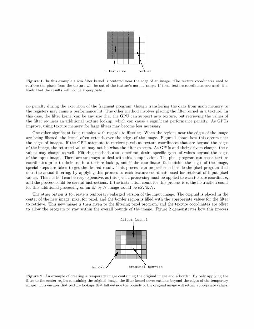
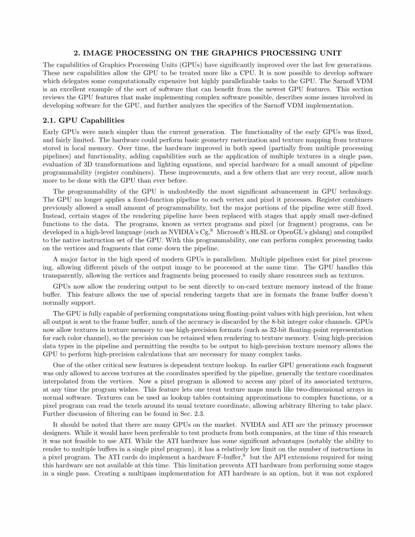
Figure 1. In this example a 5x5 filter kernel is centered near the edge of an image. The texture coordinates used toretrieve the pixels from the texture will be out of the texture’s normal range. If these texture coordinates are used, it islikely that the results will not be appropriate.

no penalty during the execution of the fragment program, though transferring the data from main memory tothe registers may cause a performance hit. The other method involves placing the filter kernel in a texture. Inthis case, the filter kernel can be any size that the GPU can support as a texture, but retrieving the values ofthe filter requires an additional texture lookup, which can cause a significant performance penalty. As GPUsimprove, using texture memory for large filters may become less necessary.

One other significant issue remains with regards to filtering. When the regions near the edges of the imageare being filtered, the kernel often extends over the edges of the image. Figure 1 shows how this occurs nearthe edges of images. If the GPU attempts to retrieve pixels at texture coordinates that are beyond the edgesof the image, the returned values may not be what the filter expects. As GPUs and their drivers change, thesevalues may change as well. Filtering methods also sometimes desire specific types of values beyond the edgesof the input image. There are two ways to deal with this complication. The pixel program can check texturecoordinates prior to their use in a texture lookup, and if the coordinates fall outside the edges of the image,special steps are taken to get the desired result. This process can be performed inside the pixel program thatdoes the actual filtering, by applying this process to each texture coordinate used for retrieval of input pixelvalues. This method can be very expensive, as this special processing must be applied to each texture coordinate,and the process could be several instructions. If the instruction count for this process is c, the instruction countfor this additional processing on an M by N image would be cSTMN .

The other option is to create a temporary enlarged version of the input image. The original is placed in thecenter of the new image, pixel for pixel, and the border region is filled with the appropriate values for the filterto retrieve. This new image is then given to the filtering pixel program, and the texture coordinates are offsetto allow the program to stay within the overall bounds of the image. Figure 2 demonstrates how this process

Figure 2. An example of creating a temporary image containing the original image and a border. By only applying thefilter to the center region containing the original image, the filter kernel never extends beyond the edges of the temporaryimage. This ensures that texture lookups that fall outside the bounds of the original image will return appropriate values.

Figure 3. Demonstration of the process to reflect texture coordinates that fall outside the area of the original image.Texture coordinates that fall inside the original image ([0..s]) are unmodified, while coordinates that fall below 0 arereflected around 0, and coordinates that fall above s are reflected around s. This demonstration is in one dimension, butthe GPU can perform this task in two dimensions at no extra cost.

prevents bad texture lookups. This method has the advantage of potentially requiring much less work per pixel,but it comes with the overhead of performing an additional pass and it requires additional texture memory. Theinstruction cost of this additional pass is roughly c(M + S)(N + T ) with an additional (M + S)(N + T ) texturereads, which are more time consuming than normal instructions.

As an example, consider a filter that is intended to reflect the image around the border. The proper texturecoordinate can be calculated by using two sets of texture coordinates, tc0 and tc1. In one dimension, if b is thesize of the border, and s is the size of the original texture, the new texture has a size of (2b) + s, the texturecoordinates represented by tc0 are in the range [−b...s+b], and the coordinates of tc1 are in the range [2s+b...s−b].By finding the maximum of tc0 and −tc0, any texture coordinates which are below zero are properly reflected.By taking the minimum of that value and tc1, texture coordinates above s are also properly reflected. A visualdemonstration of this process can be seen in Fig. 3. This process can be performed in a single pass, whichincreases the instruction count of filtering to five instructions per filter component per pixel, for a total cost of5STMN . If the border is precalculated and then the resultant image processed without the reflection checkingcode, the overall number of number of pixel instructions is approximately 3(M + S)(N + T ) + 3STMN .

3. STAGE DESCRIPTION

The stages of the GPU implementation of the Sarnoff VDM correspond fairly well to the stages described byLubin.7 The input images are monochrome, and therefore during the first few stages of the implementationthey can each be placed in a different channel of a single image. This single image containing up to four input

Figure 4. The two images used as input for the example.

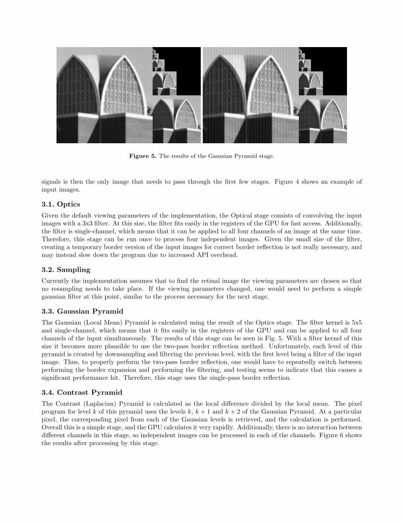
Figure 5. The results of the Gaussian Pyramid stage.

signals is then the only image that needs to pass through the first few stages. Figure 4 shows an example ofinput images.

3.1. Optics

Given the default viewing parameters of the implementation, the Optical stage consists of convolving the inputimages with a 3x3 filter. At this size, the filter fits easily in the registers of the GPU for fast access. Additionally,the filter is single-channel, which means that it can be applied to all four channels of an image at the same time.Therefore, this stage can be run once to process four independent images. Given the small size of the filter,creating a temporary border version of the input images for correct border reflection is not really necessary, andmay instead slow down the program due to increased API overhead.

3.2. Sampling

Currently the implementation assumes that to find the retinal image the viewing parameters are chosen so thatno resampling needs to take place. If the viewing parameters changed, one would need to perform a simplegaussian filter at this point, similar to the process necessary for the next stage.

3.3. Gaussian Pyramid

The Gaussian (Local Mean) Pyramid is calculated using the result of the Optics stage. The filter kernel is 5x5and single-channel, which means that it fits easily in the registers of the GPU and can be applied to all fourchannels of the input simultaneously. The results of this stage can be seen in Fig. 5. With a filter kernel of thissize it becomes more plausible to use the two-pass border reflection method. Unfortunately, each level of thispyramid is created by downsampling and filtering the previous level, with the first level being a filter of the inputimage. Thus, to properly perform the two-pass border reflection, one would have to repeatedly switch betweenperforming the border expansion and performing the filtering, and testing seems to indicate that this causes asignificant performance hit. Therefore, this stage uses the single-pass border reflection.

3.4. Contrast Pyramid

The Contrast (Laplacian) Pyramid is calculated as the local difference divided by the local mean. The pixelprogram for level k of this pyramid uses the levels k, k + 1 and k + 2 of the Gaussian Pyramid. At a particularpixel, the corresponding pixel from each of the Gaussian levels is retrieved, and the calculation is performed.Overall this is a simple stage, and the GPU calculates it very rapidly. Additionally, there is no interaction betweendifferent channels in this stage, so independent images can be processed in each of the channels. Figure 6 showsthe results after processing by this stage.

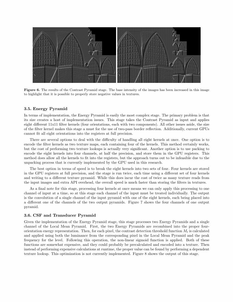
Figure 6. The results of the Contrast Pyramid stage. The base intensity of the images has been increased in this imageto highlight that it is possible to properly store negative values in textures.

3.5. Energy Pyramid

In terms of implementation, the Energy Pyramid is easily the most complex stage. The primary problem is thatits size creates a host of implementation issues. This stage takes the Contrast Pyramid as input and applieseight different 11x11 filter kernels (four orientations, each with two components). All other issues aside, the sizeof the filter kernel makes this stage a must for the use of two-pass border reflection. Additionally, current GPUscannot fit all eight orientations into the registers at full precision.

There are several options to deal with the difficulty of handling all eight kernels at once. One option is toencode the filter kernels as two texture maps, each containing four of the kernels. This method certainly works,but the cost of performing two texture lookups is actually very significant. Another option is to use packing toencode the eight kernels into four channels, at half the precision, and store them in the GPU registers. Thismethod does allow all the kernels to fit into the registers, but the approach turns out to be infeasible due to theunpacking process that is currently implemented by the GPU used in this research.

The best option in terms of speed is to break the eight kernels into two sets of four. Four kernels are storedin the GPU registers at full precision, and the stage is run twice, each time using a different set of four kernelsand writing to a different texture pyramid. While this does incur the cost of twice as many texture reads fromthe input images and extra API overhead, the overall speed is much faster than storing the filters in textures.

As a final note for this stage, processing four kernels at once means we can only apply this processing to onechannel of input at a time, so at this stage each channel of the input must be treated individually. The outputis the convolution of a single channel of the input pyramid with one of the eight kernels, each being placed intoa different one of the channels of the two output pyramids. Figure 7 shows the four channels of one outputpyramid.

3.6. CSF and Transducer Pyramid

Given the implementation of the Energy Pyramid stage, this stage processes two Energy Pyramids and a singlechannel of the Local Mean Pyramid. First, the two Energy Pyramids are recombined into the proper four-orientation energy representation. Then, for each pixel, the contrast detection threshold function Mt is calculatedand applied using both the luminance from the corresponding pixel in the Local Mean Pyramid and the peakfrequency for the level. Following this operation, the non-linear sigmoid function is applied. Both of thesefunctions are somewhat expensive, and they could probably be precalculated and encoded into a texture. Theninstead of performing expensive calculations at runtime, the proper value can be found by performing a dependenttexture lookup. This optimization is not currently implemented. Figure 8 shows the output of this stage.

Figure 7. Black and white representations of part of the output from the Energy Pyramid stage. The images show theresults of applying the four oriented Gaussian filters to the second Contrast Pyramid in Fig. 6. All four results are outputin different color channels of a single output image. a) The horizonal filter, located in the red channel of the output image.b) One of the diagonal filters, located in the blue channel of the output image. c) The vertical filter, located in the greenchannel of the output image. d) The other diagonal filter, located in the alpha channel of the output image.

Figure 8. A portion of the results of the CSF and Transducer Pyramid stage. Both images correspond to the EnergyPyramid’s vertically sensitive filters. The left image is from the perfect VDM input, and the right image is from the VDMinput with the vertical sine grating artifact. The intensity of these images has been scaled down.

Figure 9. The result of the Difference Pyramid stage. The intensity has been scaled down significantly.

3.7. Pooling Pyramid

The Pooling Pyramid is a simple stage where the value of a pixel is calculated as the average over a 5x5 regionsurrounding it. As such, it’s similar to the Gaussian Pyramid stage, but a bit simpler. It executes reasonablyfast using single-pass border reflection, so two-pass border reflection will probably not improve the speed.

3.8. Difference Pyramid

The Difference Pyramid takes two Pooling Pyramids and applies the distance calculation. The Result is a single-channel pyramid that describes the difference found in each pixel of each level. This is an intermediate stage thatexists in case the GPU can’t support the number of active textures it would require to calculate the DifferenceMap in one pass. Figure 9 shows the output from this stage.

3.9. Difference Map

The Difference Map stage takes a Difference Pyramid, upsamples all the stages to the same size, and combinesthem. This requires as many as 7 active textures, which is fine for most modern GPUs. Figure 10 shows theresults this stage, a JND Map. This stage would likely be faster if pyramids were implemented as a single texturewith multiple regions, rather than multiple textures.

Figure 10. The result of combining the levels of the Difference Pyramid. This is the JND Map depicting likely areas ofdetectable difference between the two input images. The intensity has been scaled down.

Table 1. The instruction count of each stage’s fragment program.

Stage Basic Ops Texture Reads Total Ops Multi-ImageOptics 35 9 44 YesGaussian 99 25 124 YesContrast 8 3 11 YesEnergy 245 121 366 NoCSF and Transducer 51 3 54 NoPooling 99 25 124 NoDifference 12 2 14 NoDifference Map 22 8 30 NoStatistics 14 4 18 NoBorder Creation 2 1 3 N/A

3.10. Statistics

The Difference Map is complete after the last stage has finished. However, if statistical information (such as themean, minimum and maximum) about the JND values it contains is desired, there are two choices. The entiremap can be copied to CPU memory and the appropriate values calculated, but this can be slow. The GPU canbe used for this task as well. First one places the minimum, maximum and total sum of the intensity values ofeach pixel into separate channels (this is already the case if the image is using four channels but is monochrome).Then, by repeatedly downsampling the image, the desired statistical values of two-by-two pixel regions can befound and stored in the proper channels of the smaller image. Care must be taken during the downsampling tonot include pixels at texture coordinates that are outside the actual texture. The process is complete when theresult is a single pixel with the minimum, maximum and total intensity in three of its four channels. This singlepixel can then be copied to the CPU and the mean intensity calculated, saving bandwidth and CPU processingtime.

4. COST ANALYSIS

The total cost of running the Sarnoff VDM on the GPU depends on several factors. While some of the GPUscan support a very large number of instructions per pixel, high instruction count programs do take longer torun. Texture operations can also be significantly slower than basic operations because they must fetch data frommemory. Another consideration is the ability of the various stages to process multiple inputs. The first severalstages can handle up to four monochrome input images at a time, allowing a significant savings if used. Table 1shows the instruction count of the programs for each stage using the NVIDIA FX architecture, as well as themulti-image processing capabilities.

Given the instructional cost of these stages, one must then consider the time it takes to execute them. Thefirst time a stage is executed it incurs a penalty for compiling and loading the program. Repeated applicationof the program during the same session does not incur this penalty. Timing was based on repeated execution of

Table 2. The overall running time of each implementation for a two-image comparison. *Due to an error in the Uniximplementation, this run uses a slightly simpler method of CSF calculation than the other implementations.

Time (ms)Implementation256x256 512x512

Unix Software 6060* 24750Windows Software 3734 12125Windows GPU (Go700) 680 2490Windows GPU (5900 Ultra) 320 1140

Figure 11. How total processing time is distributed among the stages.

the stages, so the initial execution time of a stage was ignored. Accurate per-stage timing information is difficultto obtain, but Fig. 11 shows the relative amount of time spent in each stage for a typical two-image input.

Processing time is easier to determine when considering the execution of the entire metric. Two test machineswere used to examine running time for the GPU implementation, a laptop and a desktop. The laptop machineis a 1.4 GHz Intel Pentium M with 1 GB of RAM, and its GPU is a NVIDIA Quadro FX Go700 with 128 MB ofRAM. The desktop machine is a dual 2.8 GHz Intel Pentium 4 with 1 GB of RAM, and its GPU is a NVIDIAGeForce FX 5900 Ultra with 256 MB of RAM.

To find the speed improvement a comparison was made against two reference software implementations.One implementation was developed under Unix,10 and the other implementation was a Windows port of theUnix implementation. The Unix machine used was a SunBlade 2000. The Windows machine used is the samemachine used for the GPU tests. The parameters for the software implementations were set to match the GPUimplementation. As can be seen in Table 2, the GPU-based solutions offer vastly improved speed, with morethan an order of magnitude difference between the fastest software implementation and the GPU implementationrunning on the GeForce Fx 5900 Ultra.

GPU texture memory did not become a factor at any time in these tests. Assuming a good layout of texturememory, a 128-bits-per-pixel pyramid with a base of 512x512 pixels should require approximately 5.33 MB ifcreated with independent images. Given the number of pyramids and images necessary for each stage, the texturememory required for a comparison of two 512x512 images is roughly 76 MB. Thus even the Laptop GPU with128 MB is sufficient.

5. CONCLUSION

Modern GPUs can clearly perform the primary tasks in complex image processing software such as the SarnoffVDM. Because of the specialized hardware, image-based algorithms or other significant matrix computations canactually perform faster on the GPU than the CPU without fear of lost accuracy. In the case of the Sarnoff VDMan order of magnitude increase in speed resulted from moving the program onto the GPU. The implementationof the Sarnoff VDM on a GPU provides a solution fast enough to be used at interactive rates, especially whencomparing images synthesized directly on the GPU. Additional improvements to the implementation, in terms

of both algorithms and programming techniques, would serve to decrease the running time. It is also likely thatfuture generations of GPUs will produce large speed improvements.

Implementing the Sarnoff VDM on a GPU makes it possible to develop a number of interesting applications.An interactive version of the Sarnoff VDM has already been written, and it allows the user to explore, in near realtime, the significance of various pictorial artifacts. If modified for motion, a visual difference metric on a nextgeneration GPU could potentially be used to process live video. A graphics card with a visual difference metricon board makes it practical to integrate complex perceptual calculations into interactive graphics applications.Novel versions of the visual difference metric itself can be developed and tested much more quickly on a GPUthan on a CPU. Moving beyond the visual difference metric paradigm, other models of human vision can beevaluated interactively, and the increasingly powerful GPU could become a new platform for vision research.

ACKNOWLEDGMENTS

This research was conducted at the University of Minnesota Digital Technology Center. Funding was providedby National Science Foundation Grant number CCR-0242757.

REFERENCES1. T. Purcell, I. Buck, W. Mark, and P. Hanrahan, “Ray tracing on programmable graphics hardware,” in

ACM Transactions on Graphics, 21(3), pp. 703–712, 2002.2. N. Carr, J. Hall, and J. Hart, “The ray engine,” in Proceedings of the ACM SIGGRAPH/EUROGRAPHICS

Workshop on Graphics Hardware, pp. 37–46, 2002.3. M. Harris, W. Baxter, T. Scheuremann, and A. Lastra, “Simulation and computation: Simulation of cloud

dynamics on graphics hardware,” in Proceedings of the ACM SIGGRAPH/EUROGRAPHICS Workshop onGraphics Hardware, pp. 92–134, 2003.

4. J. Bolz, I. Farmer, E. Grinspun, and P. Schroder, “Sparse matrix solvers on the gpu: Conjugate gradientsand multigrid,” in ACM Transactions on Graphics, 22(3), pp. 917–924, 2003.

5. J. Kruger and R. Westermann, “Linear algebra operators for gpu implementation of numerical algorithms,”in ACM Transactions on Graphics, 22(3), pp. 908–916, 2003.

6. K. Hillesland, S. Molinov, and R. Grzeszczuk, “Nonlinear optimization framework for image-based modelingon programmable graphics hardware,” in ACM Transactions on Graphics, 22(3), pp. 925–934, 2003.

7. J. Lubin, “A visual discrimination model for imaging system design and evaluation,” in Vision Models forTarget Detection and Recognition, E. Peli, ed., pp. 245–283, World Scientific, 1995.

8. W. Mark, R. Glanville, K. Akeley, and M. Kilgard, “Cg: A system for programming graphics hardware ina C-like language,” in ACM Transactions on Graphics, 22(3), pp. 896–907, 2003.

9. W. R. Mark and K. Proudfoot, “The f-buffer: A rasterization-order fifo buffer for multi-pass rendering,”in Proceedings of the ACM SIGGRAPH/EUROGRAPHICS Workshop on Graphics Hardware, pp. 57–64,2001.

10. B. Li, G. Meyer, and R. Klassen, “A comparison of two image quality models,” in Human Vision andElectronic Imaging III, B. E. Rogowitz and T. N. Pappas, eds., 3299, pp. 98–109, Proc. SPIE, (San Jose,California), 1998.