Implementation for Spatial Data of the Shared...
87
Bruno Filipe Fernandes Simões Salgueiro Faustino Licenciado em Engenharia Informática Implementation for Spatial Data of the Shared Nearest Neighbour with Metric Data Structures Dissertação para obtenção do Grau de Mestre em Engenharia Informática Orientador : Doutor João Carlos Gomes Moura Pires, Professor Auxiliar, Universidade Nova de Lisboa Júri: Presidente: Professora Doutora Ana Maria Dinis Moreira Arguente: Professora Doutora Maribel Yasmina Campos Alves Santos Vogal: Professor Doutor João Carlos Gomes Moura Pires Novembro, 2012
Transcript of Implementation for Spatial Data of the Shared...

Bruno Filipe Fernandes Simões Salgueiro Faustino
Licenciado em Engenharia Informática
Implementation for Spatial Data of the SharedNearest Neighbour with Metric Data
Structures
Dissertação para obtenção do Grau de Mestre emEngenharia Informática
Orientador : Doutor João Carlos Gomes Moura Pires,Professor Auxiliar, Universidade Nova de Lisboa
Júri:
Presidente: Professora Doutora Ana Maria Dinis Moreira
Arguente: Professora Doutora Maribel Yasmina Campos Alves Santos
Vogal: Professor Doutor João Carlos Gomes Moura Pires
Novembro, 2012


iii
Implementation for Spatial Data of the Shared Nearest Neighbour with MetricData Structures
Copyright c© Bruno Filipe Fernandes Simões Salgueiro Faustino, Faculdade de Ciênciase Tecnologia, Universidade Nova de Lisboa
A Faculdade de Ciências e Tecnologia e a Universidade Nova de Lisboa têm o direito,perpétuo e sem limites geográficos, de arquivar e publicar esta dissertação através de ex-emplares impressos reproduzidos em papel ou de forma digital, ou por qualquer outromeio conhecido ou que venha a ser inventado, e de a divulgar através de repositórioscientíficos e de admitir a sua cópia e distribuição com objectivos educacionais ou de in-vestigação, não comerciais, desde que seja dado crédito ao autor e editor.

iv

In loving memory of José Jerónimo Guerreiro Faustino andRogélia Ermelinda Salgueiro Faustino.

vi

Acknowledgements
First and foremost, I would like to express my deep gratitude to Assistant Professor JoãoMoura Pires, for relying on me with this thesis and for all his challenging and valuablequestions, useful reviews, patient guidance and encouragement, not only regarding thisthesis, but also about helping me grow as an individual. I would like to thank the Facul-dade de Ciências e Tecnologia da Universidade Nova de Lisboa for providing its studentswith such a grand campus, not only for its size and for the variety of services available onit, but also for the significant number and size of green spaces. I am particularly gratefulto the Computer Science Department for giving me a research grant in the System forAcademic Information Analysis (SAIA) project, envisioned and guided also by AssistantProfessor João Moura Pires. I wish to acknowledge and thank several other professors:Assistant Professor Maribel Yasmina Santos, for providing her knowledge about the clus-tering algorithm used in this thesis; Assistant Professor Margarida Mamede, for sharingher knowledge in metric spaces; Assistant Professor João Costa Seco, who answered somequestions regarding the interoperability of programming languages; and Assistant Pro-fessor Artur Miguel Dias, for explaining how the Java Native Interface works. I wouldalso like to thank all my colleagues that presented me with memorable moments duringthe elaboration of this thesis, namely the following: André Fidalgo, for all his supportand contributions in brainstorms; Sérgio Silva, for his support; Márcia Silva, for all thefun and unwind moments; and Manuel Santos, for helping prepare the server for theexperimental results and sharing his knowledge in emerging technologies.
Thanks to Complexo Educativo Cata-Ventos da Paz, Escola Básica D. António daCosta and Escola Secundária Cacilhas-Tejo, for the given educational background.
Thanks to the Clube Português de Caravanismo, where part of this document waswrote, for providing its campers with such sound conditions and environment.
Last, but not least, my special thanks to my parents, for the given education and forthe given support during the elaboration of this thesis. I would also like to express myspecial thanks to all the remaining family members and friends, that had an importantrole during this important moment in my life.
vii

viii

Abstract
Clustering algorithms are unsupervised knowledge retrieval techniques that organizedata into groups. However, these algorithms require a meaningful runtime and severalruns to achieve good results.
The Shared Nearest Neighbour (SNN) is a data clustering algorithm that identifiesnoise in data and finds clusters with different densities, shapes and sizes. These featuresmake the SNN a good candidate to deal with spatial data. It happens that spatial data isbecoming more available, due to an increasing rate of spatial data collection. However,the SNN time complexity can be a bottleneck in spatial data clustering, since it has a timecomplexity in the worst case evaluated in O(n2), which compromises its scalability.
In this thesis, it is proposed to use metric data structures in primary or secondary stor-age, to index spatial data and support the SNN in querying for the k-nearest neighbours,since this query is the source of the quadratic time complexity of the SNN.
For low dimensional data, namely when dealing with spatial data, the time com-plexity in the average case of the SNN, using a metric data structure in primary storage(kd-Tree), is improved to at most O(n× log n). Furthermore, using a strategy to reuse thek-nearest neighbours between consecutive runs, it is possible to obtain a time complexityin the worst case of O(n).
The experimental results were done using the kd-Tree and the DF-Tree, which workin primary and secondary storage, respectively. These results showed good performancegains in primary storage, when compared with the performance of a referenced imple-mentation of the SNN. In secondary storage, with 128000 objects, the performance be-came comparable with the performance of the referenced implementation of the SNN.
Keywords: df-tree, kd-tree, shared nearest neighbour, snn, spatial data
ix

x

Resumo
Os algoritmos de agrupamento são técnicas não supervisionadas de aprendizagemautomática, que organizam os dados em grupos. Contudo, estes algoritmos requeremum tempo de execução significativo e várias corridas para alcançar bons resultados.
O Shared Nearest Neighbour (SNN) é um algoritmo de agrupamento que identifica oruído nos dados e encontra grupos com densidades, formas e tamanhos distintos. Es-tas características fazem do SNN um bom candidato para lidar com os dados espaciais.Acontece que os dados espaciais estão cada vez mais disponíveis, por estarem a ser co-lectados a um ritmo impressionante. Contudo, a complexidade temporal do SNN podeser um obstáculo à aplicação do algoritmo sobre dados espaciais, visto que a sua comple-xidade temporal no pior caso é O(n2), o que compromete a sua escalabilidade.
Nesta dissertação, é proposto o uso de estruturas de dados métricas em memóriaprimária ou secundária, para indexar os dados e dar suporte ao SNN à consulta pelosk-vizinhos mais próximos, já que esta é a fonte da complexidade quadrática do SNN.
Para dados de baixa dimensionalidade, nomeadamente com dados espaciais, a com-plexidade temporal no caso esperado do SNN, com o recurso a uma estrutura de dadosmétrica em memória primária (kd-Tree), foi melhorada para quanto muitoO(n× log n). Sefor usada uma estratégia de reaproveitamento dos k-vizinhos mais próximos entre corri-das consecutivas, é possível obter uma complexidade no pior caso avaliada em O(n).
Foram usadas experimentalmente a kd-Tree e a DF-Tree, que funcionam em memóriaprimária e secundária, respectivamente. Os resultados demonstraram ganhos de desem-penho significativos em memória primária, em relação a uma implementação de refe-rência do SNN. Em memória secundária, com 128000 objectos, o desempenho tornou-secomparável ao desempenho da implementação de referência do SNN.
Palavras-chave: df-tree, kd-tree, shared nearest neighbour, snn, dados espaciais
xi

xii

Contents
1 Introduction 11.1 Context and Motivation . . . . . . . . . . . . . . . . . . . . . . . . . . . . . 11.2 Problem . . . . . . . . . . . . . . . . . . . . . . . . . . . . . . . . . . . . . . 31.3 Approach . . . . . . . . . . . . . . . . . . . . . . . . . . . . . . . . . . . . . . 41.4 Contributions . . . . . . . . . . . . . . . . . . . . . . . . . . . . . . . . . . . 51.5 Outline of the Document . . . . . . . . . . . . . . . . . . . . . . . . . . . . . 5
2 Clustering Algorithms 72.1 Introduction . . . . . . . . . . . . . . . . . . . . . . . . . . . . . . . . . . . . 72.2 Shared Nearest Neighbour . . . . . . . . . . . . . . . . . . . . . . . . . . . . 8
2.2.1 Parameters . . . . . . . . . . . . . . . . . . . . . . . . . . . . . . . . . 82.2.2 Algorithm . . . . . . . . . . . . . . . . . . . . . . . . . . . . . . . . . 92.2.3 Other Variants . . . . . . . . . . . . . . . . . . . . . . . . . . . . . . . 112.2.4 Synopsis . . . . . . . . . . . . . . . . . . . . . . . . . . . . . . . . . . 12
2.3 Other Clustering Algorithms . . . . . . . . . . . . . . . . . . . . . . . . . . 122.3.1 SNNAE . . . . . . . . . . . . . . . . . . . . . . . . . . . . . . . . . . 122.3.2 Chameleon . . . . . . . . . . . . . . . . . . . . . . . . . . . . . . . . 152.3.3 CURE . . . . . . . . . . . . . . . . . . . . . . . . . . . . . . . . . . . 162.3.4 DBSCAN . . . . . . . . . . . . . . . . . . . . . . . . . . . . . . . . . . 17
2.4 Evaluation of the Clustering Algorithms . . . . . . . . . . . . . . . . . . . . 182.4.1 SNN and Chameleon . . . . . . . . . . . . . . . . . . . . . . . . . . . 182.4.2 SNN and CURE . . . . . . . . . . . . . . . . . . . . . . . . . . . . . . 182.4.3 SNN and DBSCAN . . . . . . . . . . . . . . . . . . . . . . . . . . . . 19
2.5 Validation of Clustering Results . . . . . . . . . . . . . . . . . . . . . . . . . 202.6 Summary . . . . . . . . . . . . . . . . . . . . . . . . . . . . . . . . . . . . . . 21
3 Metric Spaces 233.1 Introduction . . . . . . . . . . . . . . . . . . . . . . . . . . . . . . . . . . . . 233.2 Metric Data Structures . . . . . . . . . . . . . . . . . . . . . . . . . . . . . . 24
xiii

xiv CONTENTS
3.2.1 kd-Tree . . . . . . . . . . . . . . . . . . . . . . . . . . . . . . . . . . . 263.2.2 M-Tree . . . . . . . . . . . . . . . . . . . . . . . . . . . . . . . . . . . 273.2.3 DF-Tree . . . . . . . . . . . . . . . . . . . . . . . . . . . . . . . . . . 29
4 Approach 314.1 Introduction . . . . . . . . . . . . . . . . . . . . . . . . . . . . . . . . . . . . 31
4.1.1 Implementing the SNN using Metric Data Structures . . . . . . . . 314.1.2 Architecture . . . . . . . . . . . . . . . . . . . . . . . . . . . . . . . . 33
4.2 Using the kd-Tree with the SNN . . . . . . . . . . . . . . . . . . . . . . . . . 354.2.1 Reader . . . . . . . . . . . . . . . . . . . . . . . . . . . . . . . . . . . 354.2.2 SNN . . . . . . . . . . . . . . . . . . . . . . . . . . . . . . . . . . . . 364.2.3 Output . . . . . . . . . . . . . . . . . . . . . . . . . . . . . . . . . . . 404.2.4 Time Complexity Evaluation . . . . . . . . . . . . . . . . . . . . . . 41
4.3 Using the DF-Tree with the SNN . . . . . . . . . . . . . . . . . . . . . . . . 424.3.1 C++ Reader . . . . . . . . . . . . . . . . . . . . . . . . . . . . . . . . 434.3.2 DB Reader . . . . . . . . . . . . . . . . . . . . . . . . . . . . . . . . . 434.3.3 DB Output . . . . . . . . . . . . . . . . . . . . . . . . . . . . . . . . . 44
5 Experimental Results 455.1 Data Sets . . . . . . . . . . . . . . . . . . . . . . . . . . . . . . . . . . . . . . 45
5.1.1 Synthetic . . . . . . . . . . . . . . . . . . . . . . . . . . . . . . . . . . 455.1.2 Marin Data . . . . . . . . . . . . . . . . . . . . . . . . . . . . . . . . 465.1.3 Twitter . . . . . . . . . . . . . . . . . . . . . . . . . . . . . . . . . . . 48
5.2 kd-SNN . . . . . . . . . . . . . . . . . . . . . . . . . . . . . . . . . . . . . . . 495.2.1 Evaluation of the Quality of the Clustering Results . . . . . . . . . 495.2.2 Performance Evaluation . . . . . . . . . . . . . . . . . . . . . . . . . 53
5.3 DF-SNN . . . . . . . . . . . . . . . . . . . . . . . . . . . . . . . . . . . . . . 555.3.1 Evaluation of the Quality of the Clustering Results . . . . . . . . . 555.3.2 Performance Evaluation . . . . . . . . . . . . . . . . . . . . . . . . . 58
6 Conclusions 63

List of Figures
2.1 SNN - Distances Matrix . . . . . . . . . . . . . . . . . . . . . . . . . . . . . 9
2.2 SNN Example - Graph with the 3-nearest neighbours of the 7 Objects . . . 9
2.3 SNN Example - Graph with the Similarity Values (Eps = 2) . . . . . . . . . 10
2.4 SNN Example - Graph with the Density Values (MinPts = 2) . . . . . . . . 10
2.5 SNN Example - Graph with the Clustering Results . . . . . . . . . . . . . . 11
2.6 Clusters and Noise Identified by the SNN . . . . . . . . . . . . . . . . . . . 12
2.7 Enclosures in the SNNAE . . . . . . . . . . . . . . . . . . . . . . . . . . . . 14
2.8 Runtime of the SNNAE and the Original SNN . . . . . . . . . . . . . . . . 15
2.9 Overview of the Chameleon . . . . . . . . . . . . . . . . . . . . . . . . . . . 15
2.10 Clustering Results from the SNN and the DBSCAN . . . . . . . . . . . . . 19
2.11 Studied Clustering Algorithms . . . . . . . . . . . . . . . . . . . . . . . . . 21
3.1 Metric Data Structures Taxonomy . . . . . . . . . . . . . . . . . . . . . . . . 25
3.2 Kd-Tree Example . . . . . . . . . . . . . . . . . . . . . . . . . . . . . . . . . 26
3.3 Kd-tree Time and Space Complexities . . . . . . . . . . . . . . . . . . . . . 27
3.4 M-Tree Example . . . . . . . . . . . . . . . . . . . . . . . . . . . . . . . . . . 28
3.5 DF-Tree Example . . . . . . . . . . . . . . . . . . . . . . . . . . . . . . . . . 29
3.6 DF-Tree Pruning using Global Representative . . . . . . . . . . . . . . . . . 30
4.1 Runs Taxonomy . . . . . . . . . . . . . . . . . . . . . . . . . . . . . . . . . . 32
4.2 Architecture . . . . . . . . . . . . . . . . . . . . . . . . . . . . . . . . . . . . 34
4.3 Time Complexities of the Algorithms of the SNN . . . . . . . . . . . . . . . 40
4.4 Example of an ARFF file . . . . . . . . . . . . . . . . . . . . . . . . . . . . . 41
4.5 Time Complexities of the Runs of the kd-SNN . . . . . . . . . . . . . . . . . 42
4.6 SQL File - Objects Table . . . . . . . . . . . . . . . . . . . . . . . . . . . . . 43
4.7 SQL File - k-Nearest Neighbours Table . . . . . . . . . . . . . . . . . . . . . 43
5.1 Attributes of the Synthetic Data Sets . . . . . . . . . . . . . . . . . . . . . . 45
5.2 Distribution of the Synthetic Data Sets . . . . . . . . . . . . . . . . . . . . . 46
xv

xvi LIST OF FIGURES
5.3 Subset of Attributes of the Marin Data Set . . . . . . . . . . . . . . . . . . . 475.4 Subset of Ship Types in the Marin Data Set . . . . . . . . . . . . . . . . . . 475.5 Spatial Distribution of the Marin Data Set . . . . . . . . . . . . . . . . . . . 485.6 Attributes of the Twitter Data Set . . . . . . . . . . . . . . . . . . . . . . . . 485.7 Spatial Distribution of the Twitter Data Set . . . . . . . . . . . . . . . . . . 485.8 Clustering Results of the Synthetic 1 Data Set (Evaluation of the kd-SNN) 495.9 Clustering Results of the Synthetic 2 Data Set (Evaluation of the kd-SNN) 505.10 Clustering Results of the Synthetic 3 Data Set (Evaluation of the kd-SNN) 505.11 Clustering Results of the LPG Ship Type (Evaluation of the kd-SNN) . . . 515.12 Clustering Results of the Oil Ship Type (Evaluation of the kd-SNN) . . . . 525.13 Runtime of the kd-SNN with k = 12 . . . . . . . . . . . . . . . . . . . . . . 535.14 Runtime of the kd-SNN with k = 8, k = 10 and k = 12 . . . . . . . . . . . . 545.15 Runtime of the Original SNN and of the TNC run of the kd-SNN with k = 12 555.16 Clustering Results of the Synthetic 1 Data Set (Evaluation of the DF-SNN) 555.17 Clustering Results of the Synthetic 2 Data Set (Evaluation of the DF-SNN) 565.18 Clustering Results of the LPG Ship Type (Evaluation of the DF-SNN) . . . 565.19 Clustering Results of the Oil Ship Type (Evaluation of the DF-SNN) . . . . 575.20 Runtime of the DF-SNN with k = 12 . . . . . . . . . . . . . . . . . . . . . . 595.21 Weight of Importing the SQL file to the DBMS . . . . . . . . . . . . . . . . 595.22 No. of Secondary Storage Accesses by the DF-Tree with k = 12 . . . . . . . 605.23 Runtime of the DF-SNN with k = 8, k = 10 and k = 12 . . . . . . . . . . . 615.24 Runtime of the Original SNN and of the TNC run of the DF-SNN with k = 12 62

1Introduction
This introductory chapter describes the context and motivation that lead to the mainproblem of this dissertation, defining some important concepts that need to be knowna priori. Following, there is a brief description about the approach taken to address theproblem and the resulting contributions of this approach . By the end of this chapter, it isdescribed the outline of this document.
1.1 Context and Motivation
Spatial data consists generally of low dimensional data defined by spatial attributes, forinstance, geographical location (latitude and longitude), and other attributes, for exam-ple, heading, speed or time [SKN07]. Nowadays, there is an increasing rate of spatialdata collection [SKN07], from which useful knowledge can be extracted by using ma-chine learning techniques [dCFLH04, Fer07, GXZ+11].
One widely used technique to extract knowledge from data is data clustering, be-cause it does not require a priori information. Data clustering consists in an unsupervisedknowledge retrieval technique, which forms natural groupings in a data set [DHS00].The goal is to organize a data set into groups where objects that end up in the same grouphave to be similar to each other and different from those in other groups [MG09]. Thisway, it is possible to extract knowledge from data without a priori information, makingdata clustering a must have technique already used in many well-known fields: patternrecognition, information retrieval, etc.
In order to achieve the data clustering, there are numerous data clustering algorithmsthat require distance functions to measure the similarity between objects. These functionsmight not be specific to a data set, but are at least specific to the domain or the type of the
1

1. INTRODUCTION 1.1. Context and Motivation
data set.Clustering algorithms are broadly classified, according to the type of the clustering
results [MH09]:
• Hierarchical - data objects are organized into a hierarchy with a sequence of nestedpartitions or groupings, using a bottom-up approach of merging clusters from small-er to bigger ones (dendrogram).
• Partition - data objects are divided into a number of non-hierarchical and non-overlapping partitions of groupings.
In addition, clustering algorithms can also be broken down to the following types,depending on their clustering process [GMW07]: center-based, where clusters are rep-resented by centroids that may not be real objects in a data set; search-based, where thesolution space is searched to find a globally optimal clustering that fits a data set; graph-based, where the clustering is accomplished by clustering a graph built from a data set;grid-based, where the clustering is done per cell of a grid created over a data set; anddensity-based, where clusters are defined by dense regions of objects, separated by low-density regions.
Nevertheless, the main issues in data clustering algorithms become clear, dependingon the application [ESK03]:
• How to choose the number of clusters in partition algorithms or when to stop themerging operation in hierarchical algorithms? Because we can not foresee the num-ber of clusters that fit a certain data set;
• How to identify the most appropriate similarity measure? Because the similaritybetween objects in the same cluster must be maximal and minimal when comparingobjects in different clusters;
• How to deal with noise in data? Because usually all data sets have noise (objectsthat are sparse from most objects) and they may compromise the clustering;
• How to find clusters with different shapes, sizes and densities? Because not all clus-ters have the same shape, size and density, and they need to be clearly identified;
• How to deal with the scalability? Because, as stated before, there is a tendencytowards a large amount of spatial data and this has an impact on the runtime of theclustering algorithms.
Density-based clustering algorithms are a good option to help solve some of the aboveissues. In density-based clustering algorithms, the clusters can be found with arbitraryshapes, having higher or lower density. This way, some of the objects in lower densityregions can be defined as noise, since they are more sparse from the rest. An example ofa density-based clustering algorithm is the Shared Nearest Neighbour (SNN) [ESK03].
2

1. INTRODUCTION 1.2. Problem
The SNN is a partition density-based clustering algorithm that uses the k-nearestneighbours of each object in a data set in its similarity measure. The SNN requires threeuser-defined parameters:
• k - the number of neighbours;
• ε (Eps) - the similarity threshold that tries to keep connections between uniformregions of objects and break connections between transitional regions, enabling theSNN to handle clusters with different densities, shapes and sizes;
• MinPts - the density threshold that helps the SNN to deal with noise, because whenit is met, the objects are representative. Otherwise, they are likely to be be noise ina data set.
Unlike some clustering algorithms (e.g. K-Means [Mac67], CURE [GRS98]), the SNNdoes not need a predetermined number of clusters, as it discovers the number by itself,giving it freedom to find the natural number of clusters, according to a data set and theuser-defined parameters. Aside from this advantage, the SNN is also a good clusteringalgorithm because, it identifies noise in a data set and deals with clusters with differentdensities, shapes and sizes, which is good, because it is not restricted to certain types ofclusters.
Some found applications using the SNN, support it: “In this experiment, we observethat there is correlation between the level of noise and the learning performance of multifocallearning.” ([GXZ+11]); “This algorithm particularly fits our needs as it automatically determinesthe number of clusters – in our case the number of topics of a text – and does not take into accountthe elements that are not representative of the clusters it builds.” ([Fer07]). More recently,there was also an application of the SNN over a spatial data set, regarding maritimetransportation trajectories, discovering distinct paths taken by ships [SSMPW12].
However, the SNN has a bottleneck that compromises its scalability: its time complex-ity, which is essentially due to the k-nearest neighbours query executed for each object ina data set. In the worst case, the query needs to travel through all the objects for each ob-ject. Therefore, the time complexity in the worst case scenario is, in the Big O Notation,O(n2), where n represents the number of objects in a data set.
The main goal of this thesis is to improve the scalability of the SNN when dealingwith spatial data, by improving its time complexity.
1.2 Problem
Regardless of the type of the clustering results or of the clustering process, some cluster-ing algorithms require the k-nearest neighbours of each object in a data set for its clus-tering process. For instance, the Chameleon algorithm (hierarchical and graph-based)[KHK99] and the Shared Nearest Neighbour (SNN) (partition and density-based) [ESK03].The scalability problem of these clustering algorithms that need to query for the k-nearest
3

1. INTRODUCTION 1.3. Approach
neighbours of each object has to be addressed in order to improve their efficiency. How-ever, the following issues should also be borne in mind, since they also have a significantimpact on the performance of the clustering algorithms:
• Storage - where to store a data set to be clustered: primary or secondary storage.Choosing the type of storage is important, not only because sometimes the data setsare to huge to be simply fit in primary storage, but also due to the time constraintsassociated with each of these types of storage. Primary storage operations (readand write) are faster than secondary storage operations by a factor of 105 or more(with the current technology) [Bur10]. Since clustering algorithms need to access adata set, it is important to choose where to store it, because if it resorts to secondarystorage, the secondary storage access speed is meaningful and must be accountedin the runtime of the clustering algorithm.
• Fine-tuning of Parameters - the clustering algorithms require user-defined parame-ters that have significant impact in the clustering results, as it will be seen in chapter2. These user-defined parameters need to be changed and adapted according to adata set being clustered, through out a sequence of runs. This is the only way tobe certain and to find the right user-defined parameters that give output to the bestpossible clustering results for a given data set. This can be a time consuming op-eration, since the algorithms need significant time to compute and to cluster all theobjects in a data set on every single run, reinforcing the importance that the timecomplexity has on the scalability of the clustering algorithms.
In view of the SNN, to achieve an improvement in its scalability, besides dealing withthe scalability problem of the k-nearest neighbours queries, the above points are alsogoing to be considered, in order to improve the performance of the SNN through out asequence of runs needed to achieve the best possible clustering results over a data set.
There is already one variant of the SNN that tries to improve its scalability. Thisvariant is called, the Shared Nearest Neighbour Algorithm with Enclosures (SNNAE)[BJ09]. It creates enclosures in a data set to outline the range of the k-nearest neighboursquery for each object, so it does not need to go through all the objects, only going throughthe ones in the same enclosure. However, the time complexity in the worst case of theSNNAE is evaluated in O(n × e + s2 × e + n × s), which is still O(n2), as s = n
e , wheree and s represent the number of enclosures and the average number of objects in eachenclosure, respectively.
1.3 Approach
The approach taken to achieve an improvement relies on metric spaces. A metric space isrepresented by a data set and a distance function, which provides support on answeringsimilarity queries: range queries or k-nearest neighbours queries.
4
1. INTRODUCTION 1.4. Contributions
Data in metric spaces is indexed in appropriate metric data structures. These struc-tures can be stored in primary or secondary storage and, depending on the type anddimensionality of a data set, can be generic or not.
Building a metric data structure, i.e. indexing a data set, takes a significant runtime,but once built, they can be reused and some can be updated, avoiding the runtime re-quired to build the structure with a data set all over again.
The goal is to improve the scalability of the SNN over spatial data, by combining theSNN with metric data structures, taking advantage of their capability of answering thek-nearest neighbours queries of the SNN, and by reusing the metric data structure andthe queries results among consecutive runs.
Some clustering algorithms already use metric data structures, for example: the au-thors of Chameleon [KHK99] state that its time complexity can be reduced from O(n2)
using metric data structures; CURE [GRS98] has a worst case time complexity of O(n2 ×log n) and uses a metric data structure to store representative objects for every cluster;and DBSCAN [EKSX96] takes full advantage of a metric data structure, in order to re-duce its time complexity from O(n2) to O(n× log n).
1.4 Contributions
The contribution of this thesis is an implementation of the SNN that:
• uses metric data structures in primary or secondary storage that give support to thek-nearest neighbours queries of the SNN;
• uses generic distance functions or specific distance functions more appropriate forspatial data;
• has its time complexity evaluated, when working in primary storage;
• has the quality of its clustering results evaluated by comparing its results with re-sults referenced in the literature;
• has its scalability evaluated by using a spatial dataset with a meaningful size and bycomparing its performance with a referenced implementation of the original SNN.
1.5 Outline of the Document
The rest of the document is organized in six chapters. The related work is divided in twochapters, due to the importance of each presented subject: in chapter 2 it is explained thebasic concepts about clustering algorithms and some clustering algorithms are detailed;in chapter 3 important properties about metric spaces and metric data structures are ex-plained and some metric data structures are also detailed. On chapter 4, the approachtaken regarding the use of metric data structures in primary or secondary storage with
5

1. INTRODUCTION 1.5. Outline of the Document
the SNN is explained. The experimental results are disclosed in chapter 5, where theevaluation of the quality and validity of the clustering results is made, and the perfor-mance of this approach is evaluated. Finally, in chapter 6 the conclusions are taken andthe future work is unveiled.
6
2Clustering Algorithms
This chapter details some concepts of clustering algorithms and explains the main clus-tering algorithm in this thesis, the SNN, and other clustering algorithms: SNNAE, Chame-leon, CURE and DBSCAN.
2.1 Introduction
A data set D = {x1, . . . , xn} is a collection of n objects. The object xi = (xi,1, . . . , xi,dim)
is described by dim attributes, where xi,j denotes the value for the attribute j of xi[GMW07].
Clustering requires the evaluation of the similarity between objects in a data set. Themost obvious similarity measure is the distance between two objects. If the distanceis a good measure of similarity, it is expected that the distance between objects in thesame cluster is smaller and it is bigger between objects in different clusters [DHS00].Given a data set, it is a hard task to choose which distance function to use to evaluate thesimilarity between objects .
A Minkowski distance is an example of a widely used family of generic distance func-tions [SB11]. Given x and y that represent two points in a dim-space and a p ≥ 1 (in orderto hold the properties of a metric), a Minkowski distance is defined by:
Lp(x, y) =
( dim∑i=1
|xi − yi|p)1/p
. (2.1)
7

2. CLUSTERING ALGORITHMS 2.2. Shared Nearest Neighbour
When p = 1, we get a well-known distance function, the Manhattan distance:
L1(x, y) =dim∑i=1
|xi − yi|. (2.2)
And when p = 2, we obtain the most common and generic distance function [ESK03],the Euclidean distance, where x and y represent two points in a euclidean dim-space:
L2(x, y) =
√√√√dim∑i=1
(xi − yi)2 =√
(x1 − y1)2 + . . .+ (xdim − ydim)2. (2.3)
However, the Euclidean distance function is not always the best, as it does not workwell when a data set that is being clustered has high dimensionality, because same objectsin the data set are sparser and their differences might be very small to distinguish with.This fact is even more noticeable with some types of data, for instance: binary types[ESK03]. Therefore, the chosen distance function must be suited for a data set and this iswhy choosing a distance function is not a simple task.
Another task is choosing the right user-defined parameters that the algorithms needbefore they start clustering a data set. These user-defined parameters have impact on theclustering results, so they need to be chosen with advisement, i.e. density, shape and sizeof clusters identified depends not only in the algorithm itself, but also on the user-definedparameters [RPN+08].
Afterwards, as clustering algorithms are an unsupervised learning technique andthere might not be predefined classes or examples that can help validate the clusteringresults, it becomes necessary an evaluation from an expert user in the application domainor the use of cluster validity measures that measure if the found clustering results are ac-ceptable or not. These cluster validity measures may be generic (explained in more detailon section 2.5) or specific to the application domain.
2.2 Shared Nearest Neighbour
The Shared Nearest Neighbour (SNN), introduced by Jarvis and Patrick [JP73], is a par-tition density-based clustering algorithm that uses the number of shared nearest neigh-bours between objects as a similarity measure.
Later, the SNN was improved with a density measure, so the algorithm could handlenoise and clusters with different densities, shapes and sizes [ESK03].
2.2.1 Parameters
The initialization of the algorithm requires the following user-defined parameters:
• k - the number of neighbours;
8

2. CLUSTERING ALGORITHMS 2.2. Shared Nearest Neighbour
• ε (Eps) - the minimum similarity between two objects. It tries to keep connectionsbetween uniform regions of objects and break connections between transitional re-gions;
• MinPts - the minimum density of an object. It is used to determine if an object isrepresentative or is likely to be noise in a data set.
Besides these user-defined parameters, the algorithm needs a distance function to beused in the k-nearest neighbours queries for each object.
2.2.2 Algorithm
The SNN algorithm starts by computing a n×nmatrix with the distances between all pairof objects in a data set (Figure 2.1). In order to measure these distances, the SNN usesa generic or a specific distance function defined by the user. Afterwards, by using thismatrix and the k value defined also by the user, the SNN is able to obtain the k-nearestneighbours of each object, by keeping the k objects in each row with the smallest distancevalues.
1 2 . . . n
1 d(1, 1) d(1, 2) . . . d(1, n)2 d(2, 1) d(2, 2) . . . d(2, n)...
......
. . ....
n d(n, 1) d(n, 2) . . . d(n, n)
Figure 2.1: SNN - Distances Matrix
Figure 2.2: SNN Example - Graph with the 3-nearest neighbours of the 7 Objects
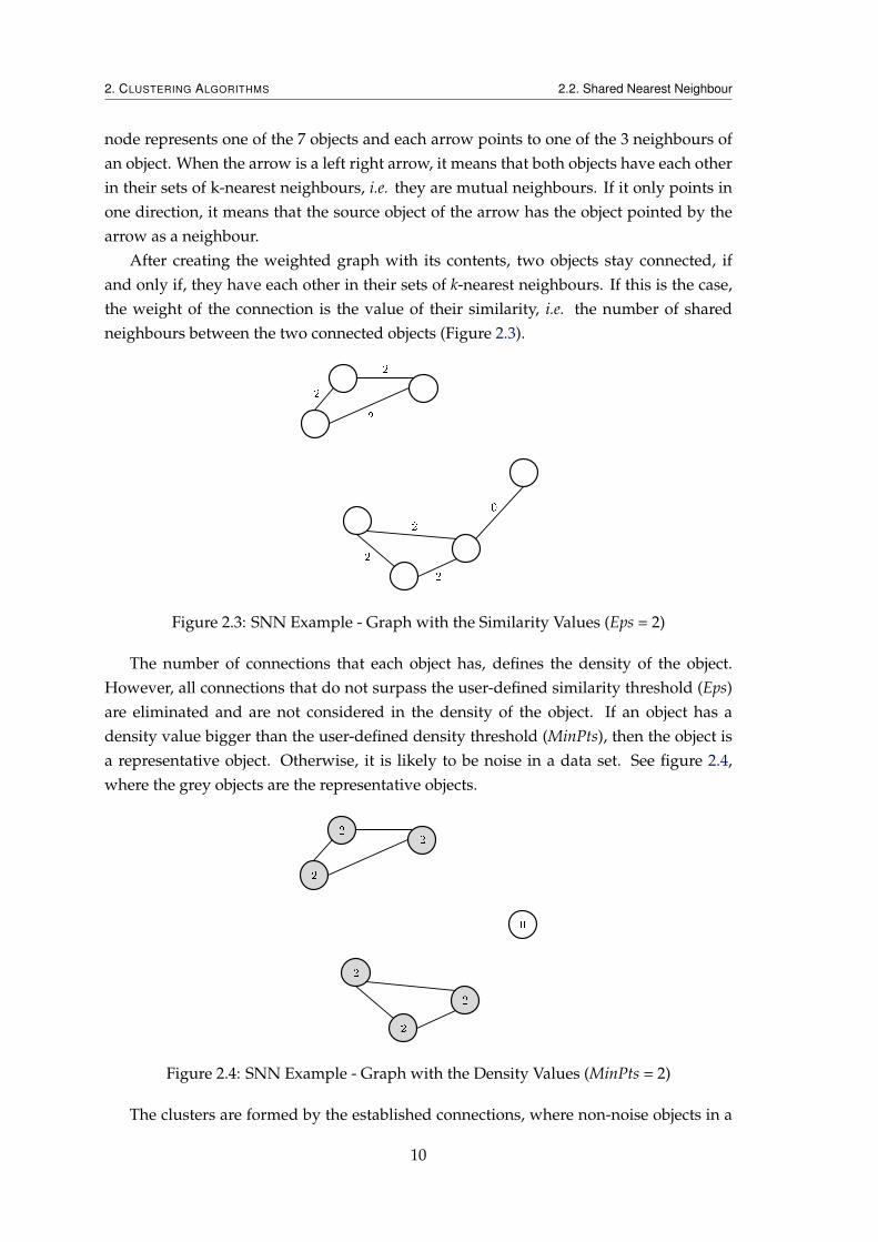
After obtaining the k-nearest neighbours of each object, a weighted graph is createdwith all the objects in the data set and with each of them connected to all their respectivek-nearest neighbours, as seen in the example in figure 2.2. The example in figure 2.2 isrepresented by a data set with 7 objects and their respective 3-nearest neighbours. Each
9
2. CLUSTERING ALGORITHMS 2.2. Shared Nearest Neighbour
node represents one of the 7 objects and each arrow points to one of the 3 neighbours ofan object. When the arrow is a left right arrow, it means that both objects have each otherin their sets of k-nearest neighbours, i.e. they are mutual neighbours. If it only points inone direction, it means that the source object of the arrow has the object pointed by thearrow as a neighbour.
After creating the weighted graph with its contents, two objects stay connected, ifand only if, they have each other in their sets of k-nearest neighbours. If this is the case,the weight of the connection is the value of their similarity, i.e. the number of sharedneighbours between the two connected objects (Figure 2.3).
Figure 2.3: SNN Example - Graph with the Similarity Values (Eps = 2)
The number of connections that each object has, defines the density of the object.However, all connections that do not surpass the user-defined similarity threshold (Eps)are eliminated and are not considered in the density of the object. If an object has adensity value bigger than the user-defined density threshold (MinPts), then the object isa representative object. Otherwise, it is likely to be noise in a data set. See figure 2.4,where the grey objects are the representative objects.
Figure 2.4: SNN Example - Graph with the Density Values (MinPts = 2)
The clusters are formed by the established connections, where non-noise objects in a
10

2. CLUSTERING ALGORITHMS 2.2. Shared Nearest Neighbour
cluster are representative or are connected directly or indirectly to a representative object.The objects that do not verify these properties are finally declared as noise (Figure 2.5,where each color represents a distinct cluster).
Figure 2.5: SNN Example - Graph with the Clustering Results
This approach will be referenced in this document as the Original SNN.
2.2.3 Other Variants
In [MSC05] the SNN and the DBSCAN, as representatives of density-based clusteringalgorithms, are analysed. The authors show some proposed variants of the SNN, namelya representative object-based approach and another one based on graphs. The authorsalso show that the results obtained with these variants are very similar to each other andvery similar to the Original SNN.
The representative objects-based approach differs in how the clustering is done. Afteridentifying the representative objects, it starts by clustering them, checking the propertiesneeded to connect two objects. Then, all non representative objects that are not in a radiusof Eps of a representative object, are defined as noise. Finally, non representative objectsthat were not defined as noise, are clustered in the cluster of the representative objectwith which they share the biggest similarity.
The graph-based approach follows the essence of the Original SNN, only divergingin how the noise is identified. After identifying the representative objects, an object is de-fined as noise, if it is not in a radius of Eps of a representative object. Then, the clusteringis done in the same way as the Original SNN. Objects in a cluster are not noise, and arerepresentative or are directly or indirectly connected to a representative object, checkingthe necessary properties to establish a connection between two objects.
Regardless of the approach, the Original SNN or one of these found variants, thetime complexity in the worst case of the SNN is O(n2), where n represents the numberof objects in a data set. This time complexity is associated with the need to compute adistances matrix to obtain the k-nearest neighbours.
With the purpose of improving this limitation, comes another variant of the SNN,
11

2. CLUSTERING ALGORITHMS 2.3. Other Clustering Algorithms
the Shared Nearest Neighbours Algorithm with Enclosures (SNNAE) [BJ09] (explainedin more detail on section 2.3.1).
2.2.4 Synopsis
The SNN is a partition density-based clustering algorithm that:
• Does not need the number of clusters as an user-defined parameter, discovering byitself the natural number of clusters, according to the contents of a data set and theuser-defined parameters;
• Deals with noise (Figure 2.6, based on [ESK03], where the red dots and the bluedots, point out the noise and the clustered objects, respectively);
Figure 2.6: Clusters and Noise Identified by the SNN
• Finds clusters with different densities, shapes and sizes.
However, the SNN has a:
• Space complexity of O(n2), due to the space occupied by the matrix with the dis-tances between objects;
• Time complexity in the worst case of O(n2), due to the operation that fills the ma-trix with all the distances between all pairs of objects, in order to get the k-nearestneighbours of each object.
2.3 Other Clustering Algorithms
On this theoretical research, several algorithms were studied: SNNAE [BJ09], Chameleon[KHK99], CURE [GRS98] and DBSCAN [EKSX96]. These algorithms were chosen, be-cause they are briefly introduced in [ESK03] and some are also tested against the OriginalSNN.
2.3.1 SNNAE
The SNNAE is a partition density-based clustering algorithm and is a variant of the Orig-inal SNN. This approach tries to make the k-nearest neighbours queries more efficient bycreating enclosures over a data set, since these queries are the source of the quadratic time
12
2. CLUSTERING ALGORITHMS 2.3. Other Clustering Algorithms
complexity of the Original SNN. The purpose of these enclosures is to limit the range ofsearch for the k-nearest neighbours of an object, requiring less distance calculations anda smaller runtime, since less objects are queried about their distances to another object.
In order to create the enclosures, the algorithm requires a less expensive distancefunction to calculate the division of data in overlapping enclosures. Then, the SNNAEuses a more expensive distance function to find the k-nearest neighbours, only inside theenclosure of the queried object.
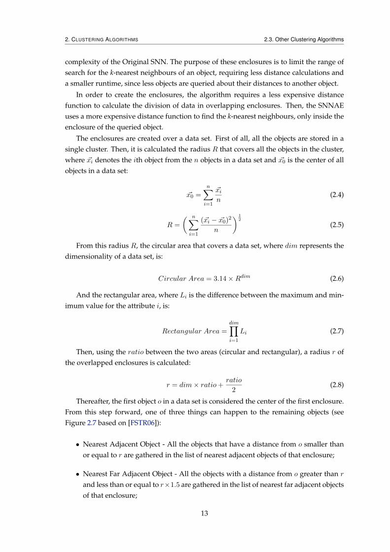
The enclosures are created over a data set. First of all, all the objects are stored in asingle cluster. Then, it is calculated the radius R that covers all the objects in the cluster,where ~xi denotes the ith object from the n objects in a data set and ~x0 is the center of allobjects in a data set:
~x0 =
n∑i=1
~xin
(2.4)
R =
( n∑i=1
(~xi − ~x0)2
n
) 12
(2.5)
From this radius R, the circular area that covers a data set, where dim represents thedimensionality of a data set, is:
Circular Area = 3.14×Rdim (2.6)
And the rectangular area, where Li is the difference between the maximum and min-imum value for the attribute i, is:
Rectangular Area =dim∏i=1
Li (2.7)
Then, using the ratio between the two areas (circular and rectangular), a radius r ofthe overlapped enclosures is calculated:
r = dim× ratio+ratio
2(2.8)
Thereafter, the first object o in a data set is considered the center of the first enclosure.From this step forward, one of three things can happen to the remaining objects (seeFigure 2.7 based on [FSTR06]):
• Nearest Adjacent Object - All the objects that have a distance from o smaller thanor equal to r are gathered in the list of nearest adjacent objects of that enclosure;
• Nearest Far Adjacent Object - All the objects with a distance from o greater than rand less than or equal to r×1.5 are gathered in the list of nearest far adjacent objectsof that enclosure;
13

2. CLUSTERING ALGORITHMS 2.3. Other Clustering Algorithms
• Center of the Next Enclosure - All the objects whose distance from o is greater thanr × 1.5 and less than r × 2 are considered to be as center of the next enclosure.
Figure 2.7: Enclosures in the SNNAE
Following the creation of the enclosures, the next step is to find the optimal valuefor ε (Eps). In the SNNAE, the Eps is calculated dynamically, instead of being a user-defined parameter like in the Original SNN. Eps is calculated by evaluating the distancesbetween every pair of objects in one enclosure, in order to find the maximum distance inone enclosure. This process is repeated for all enclosures. Then, Eps becomes the averageof the maximum distances in the enclosures.
In the final step, the Original SNN algorithm is applied, but this time, the algorithmonly searches for the k-nearest neighbours over the enclosure of the queried object.
The user-defined parameters of the SNNAE are:
• k - the number of neighbours;
• MinPts - the minimum density of an object. It is used to determine if an object isrepresentative or is likely to be noise in a data set.
Besides these user-defined parameters, the SNNAE also requires a less expensive dis-tance function for the creation of the enclosures and a more expensive distance functionto obtain the k-nearest neighbours.
According to the authors, the SNNAE is more scalable, more efficient and obtains bet-ter clustering results than the Original SNN. However, it is hard to verify these assertions,since the experimental results in [BJ09] were carried out with a very small data set evenwhen the purpose is to validate the scalability improvement obtained with the SNNAE.Some possible conclusions are drawn from figure 2.8, taken from [BJ09], where it can beseen that the SNNAE takes less half of the time finding the k-nearest neighbours, onlytaking a little more time calculating the initial clusters and composing the final clusters,when using a data set with 209 objects, each with 7 integer attributes.
14

2. CLUSTERING ALGORITHMS 2.3. Other Clustering Algorithms
5.1 Dataset Descr iption
The datasets used are db1, fish_datasest, abalone, and cpu_data. These datasets vary in size and number of attributes (dimensions). The brief description of each dataset used in the evaluation of this algorithm and the SNN algorithm is shown in Tab. 1.
Table 1. Details of datasets usedDataset Instances Attributes Data Type Cpu 209 7 Real Fish 1100 2 Synthetic Abalone 4177 7 Real Db1 10000 2 Synthetic
5.2 Implementation of SNN and SNNAE
Part of the analysis is included in the paper. The implementation is on the first dataset Cpu. The parameter values calculated using the SNNAE algorithm for creating first the enclosures and then the main clusters is depicted in Tab. 2. In Tab. 3 a comparison in terms of execution time between the SNN and the SNNAE algorithm at each step of execution is shown.
Table 2. Parameter values calculated using SNNAE
Radius of all data 0.116 Radius of enclosure 0.076 Number of enclosures 25 Eps 0.0272
Table 3. Output for MinPts 3 and all possible neighbors
Functionality SNN (Time taken
in sec.)
SNNAE (Time taken in
sec.) Find nearest neighbors
0.125 0.047
Find shared nearest neighbors
0.031 0.031
Identify core points 0 0 Get initial clusters 0 0.016 Get border and noise points
0.015 0.015
Compose cluster 0.016 0.032 Total time: 0.187 0.141
In Fig. 3, the graph shows the comparison in execution of the SNN and SNNAE algorithms as per the values shown in Tab. 3. SNNAE clearly shows more time efficiency.
00.020.040.060.080.1
0.120.14
Execution Time For cpu_data With MinPts = 3 and K = all
Find n
eares
t ne ig
hbors
Find s
hared
neare
st ne
ighbo
rs
Identi
fy cor
e poin
ts
Get init
ial clu
sters
Get bo
rder a
nd no
ise po
ints
Compo
se clu
ster
SNNSNNAE
The distribution of points in the clusters created by the SNN and the SNNAE are shown in Tab. 4. The 0th
cluster in Tab. 4 depicts the noisy data.
Table 4. Points distribution for MinPts 3
Cluster No. % of points with SNN
% of points with SNNAE
0 35.89 35.89
1 1.91 1.91
2 47.85 47.85
3 6.22 6.22
4 2.39 2.39
5 2.87 2.87
6 2.87 2.87
Total 100 100
In this way, both the algorithms are executed by varying the minimum points and numbers of points in the nearest neighborhood for each point. This is done for each dataset described in Tab. 1. The final result for the Cpu dataset is shown in Tab. 5 where for eight different sets of values both the algorithms are compared in terms of execution time.
Exe
cuti
on T
ime
in S
ec.
Task Performed
445440
Figure 2.8: Runtime of the SNNAE and the Original SNN
Regarding the quality of the clustering results, these are not shown and are not com-pared with the ones obtained with the Original SNN, making it hard to check if they arebetter or not.
The time complexity of the SNNAE in the worst case is evaluated in O(n × e + s2 ×e+ n× s), where e and s represent the number of enclosures and the average number ofobjects in each enclosure, respectively. However, since s is the average number of objectsper enclosure, i.e. s = n
e , we can deduce that the time complexity of the SNNAE is alsoquadratic, O(n2).
2.3.2 Chameleon
The Chameleon is a two-phase hierarchical clustering algorithm (Figure 2.9, taken from[KHK99]).
It starts by creating a list of the k-nearest neighbours of each object in a data set. Then,using the just filled list, a graph is constructed, where each node represents an object andconnects to another, if and only if, both nodes have each other in their sets of k-nearestneighbours.
Data SetK-nearest Neighbor Graph Final Clusters
Sparse GraphConstruct a
Merge PartitionsPartition the Graph
Figure 6: Overall framework CHAMELEON.
The key feature of CHAMELEON’s agglomerative hierarchical clustering algorithm is that it determines the pair of
most similar sub-clusters by taking into account both the inter-connectivity as well as the closeness of the clusters;
and thus it overcomes the limitations discussed in Section 3 that result from using only one of them. Furthermore,
CHAMELEON uses a novel approach to model the degree of inter-connectivity and closeness between each pair of
clusters that takes into account the internal characteristics of the clusters themselves. Thus, it does not depend on a
static user supplied model, and can automatically adapt to the internal characteristics of the clusters being merged.
In the rest of this section we provide details on how to model the data set, how to dynamically model the similarity
between the clusters by computing their relative inter-connectivity and relative closeness, how graph partitioning is
used to obtain the initial fine-grain clustering solution, and how the relative inter-connectivity and relative closeness
are used to repeatedly combine together the sub-clusters in a hierarchical fashion.
4.2 Modeling the Data
Given a similarity matrix, many methods can be used to find a graph representation [JP73, GK78, JD88, GRS99]. In
fact, modeling data items as a graph is very common in many hierarchical clustering algorithms. For example, ag-
glomerative hierarchical clustering algorithms based on single link, complete link, or group averaging method [JD88]
operate on a complete graph. ROCK [GRS99] first constructs a sparse graph from a given data similarity matrix using
a similarity threshold and the concept of shared neighbors, and then performs a hierarchical clustering algorithm on
the sparse graph. CURE [GRS98] also implicitly employs the concept of a graph. In CURE, when cluster representa-
tive points are determined, a graph containing only these representative points is implicitly constructed. In this graph,
edges only connect representative points from different clusters. Then the closest edge in this graph is identified and
the clusters connected by this edge is merged.
CHAMELEON’s sparse graph representation of the data items is based on the commonly used k-nearest neighbor
graph approach. Each vertex of the k-nearest neighbor graph represents a data item, and there exists an edge between
two vertices, if data items corresponding to either of the nodes is among the k-most similar data points of the data
point corresponding to the other node. Figure 7 illustrates the 1-, 2-, and 3-nearest neighbor graphs of a simple data
set. Note that since CHAMELEON operates on a sparse graph, each cluster is nothing more than a sub-graph of the
original sparse graph representation of the data set.
There are several advantages of representing data using a k-nearest neighbor graph G k . Firstly, data points that are
far apart are completely disconnected in the Gk . Secondly, Gk captures the concept of neighborhood dynamically.
The neighborhood radius of a data point is determined by the density of the region in which this data point resides.
In a dense region, the neighborhood is defined narrowly and in a sparse region, the neighborhood is defined more
widely. Compared to the model defined by DBSCAN [EKSX96] in which a global neighborhood density is specified,
Gk captures more natural neighborhood. Thirdly, the density of the region is recorded as the weights of the edges. The
edge weights of dense regions in Gk (with edge weights representing similarities) tend to be large and the edge weights
6
Figure 2.9: Overview of the Chameleon
In the next step, it uses a partition algorithm that splits the graph in smaller clus-ters. Then, it applies a hierarchical algorithm that finds the genuine clusters by merging
15

2. CLUSTERING ALGORITHMS 2.3. Other Clustering Algorithms
smaller ones together. In order to do this, the algorithm uses the interconnectivity be-tween clusters and their nearness, measured by thresholds and conditions imposed at theinitial parametrization of the Chameleon. This hierarchical phase stops when a schemeof conditions can no longer be verified. There are two types of schemes implemented inthe Chameleon:
• The first one only merges two clusters that have their interconnectivity and near-ness above some user-defined thresholds: TInterconnectivity and TNearness;
• The second scheme uses a function (2.9) that combines the value of the interconnec-tivity and nearness of a pair of clusters, merging the pair of clusters that maximizesthe function.
Interconnectivity(Clusteri, Clusterj)×Nearness(Clusteri, Clusterj)α. (2.9)
This function needs another user-defined parameter named α. If α is bigger than 1,then the Chameleon gives more importance to the nearness of clusters. Otherwise,it gives more importance to their interconnectivity.
The user-defined parameters of the Chameleon are:
• k - the number of neighbours;
• MinSize - the minimum granularity of the smaller clusters acquired after applyingthe initial partition algorithm;
• α - used to control the interconnectivity and nearness of clusters on the secondscheme.
Beyond these user-defined parameters, the algorithm needs a distance function tofind the k-nearest neighbours and, as already pointed out, a scheme of conditions to beused in the hierarchical phase of the Chameleon.
2.3.3 CURE
The CURE is a hierarchical clustering algorithm.The CURE starts by creating a cluster for each single object in a data set. From this
step forward, it merges the clusters that are nearer. To do so, it needs to calculate thedistance from these clusters by using their representative objects.
In the CURE a representative object is a central object of the cluster. To find the set ofrepresentative objects of a cluster, it starts by identifying well scattered objects that forman area (outline) of the cluster. Then, by closing in on the area by a fraction of α, it getsdown to the central objects of the cluster.
Now, it calculates the distance from a representative object from the set of represen-tative objects of a cluster and one from the set of another cluster. This step is repeated for
16

2. CLUSTERING ALGORITHMS 2.3. Other Clustering Algorithms
all pairs of representative objects in the sets of a pair of clusters, until it finds the mini-mum distance between two clusters in evaluation. After finding the minimum distancebetween all the clusters, it merges the ones that are closer to each other.
All the previous operations are repeated until it cuts down the number of clusters toa user-defined number.
The user-defined parameters of the CURE are:
• α - the fraction used to close in on the area;
• K - the number of clusters.
Besides these user-defined parameters, the CURE also requires a distance function toevaluate the distance between representative objects.
2.3.4 DBSCAN
The DBSCAN is a partition density-based clustering algorithm. For each single objectin a cluster, its Eps-neighbourhood must have at least a user-defined number of objects(MinPts). The shape of its Eps-neighbourhood is determined by the distance functionused.
To reach the notion of a cluster, in the context of the DBSCAN, the following defini-tions must be met:
• Eps-neighbourhood - the objects inside a radius ≤ Eps of an object o:
NEps(o) = p ∈ D | d(o, p) ≤ Eps (2.10)
, where D represents a data set, p another object and d the distance function chosen.
• Directly Density-Reachable - an object o is directly density-reachable from anotherobject p, if:
o ∈ NEps(p) ∧ |NEps(p)| ≥MinPts. (2.11)
• Density-Reachable - an object o is density-reachable from another object p if a chainof objects o1, o2, . . . , on, o1 = p, on = o exists, such that oi+1 is directly density-reachable from oi;
• Density-Connected - an object o is density-connected to a another object p if anobject q exists in a such a way that both o and p are density-reachable from q;
• Cluster - finally, in order to obtain a cluster, the following properties must be veri-fied:
∀o, p : if o ∈ C and p is density-reachable from o, then p ∈ C (2.12)
∀o, p ∈ C : o is density-connected to p (2.13)
17
2. CLUSTERING ALGORITHMS 2.4. Evaluation of the Clustering Algorithms
, where C represents a cluster.
• Noise - objects that did not fit into any cluster are defined as noise:
∀o ∈ D | ∀i : o /∈ Ci (2.14)
, where i represents the number of clusters found.
The DBSCAN starts with an arbitrary object that has not yet been visited and obtainsall its density-reachable objects. If MinPts is met, then a cluster is created. Otherwise, acluster is not created and the object is marked as visited. The algorithm stops when thereare no more objects that can be fit into clusters.
The user-defined parameters of the DBSCAN are:
• Eps - the radius of the neighbourhood;
• MinPts - the minimum number of objects required to form a cluster.
Besides these user-defined parameters, the algorithm needs a distance function to getthe objects inside the Eps-neighbourhood of an object.
2.4 Evaluation of the Clustering Algorithms
In this section, all of the presented clustering algorithms in 2.3 are compared with theOriginal SNN.
2.4.1 SNN and Chameleon
One downside of the Chameleon, where compared to the SNN, is that it does not workwell with high dimensionality data (e.g documents) [ESK03], because distances or simi-larities between objects become more uniform, making the clustering more difficult. Onthe other hand, the SNN promises a way to deal with this issue by, not only using a simi-larity measure that uses the number of shared neighbours between objects, but also usinga density measure that helps to handle the problems with similarity that can arise whendealing with high dimensionality problems.
2.4.2 SNN and CURE
When comparing the CURE with the SNN, there are three drawbacks that the CURE hasand the SNN has not. First, the user needs to define the number of clusters, as the CUREdoes not naturally discover the number, according to the remaining user-defined param-eters. Discovering the number of clusters naturally can be good in some applications (e.g.[Fer07]). Second, the CURE has a limited set of parameters which, despite of making eas-ier the fine-tuning, restricts the control over the clustering algorithm and, consequently,
18

2. CLUSTERING ALGORITHMS 2.4. Evaluation of the Clustering Algorithms
its clustering results. Third, the CURE handles many types of non-globular clusters, butit cannot handle many types of globular shaped clusters [ESK03]. This is a consequenceof finding the objects along the outline of the cluster and then shrinking the area of theoutline towards the center. Whereas, the SNN is able to identify clusters with differentdensities, shapes and sizes, without compromising any of them.
2.4.3 SNN and DBSCAN
In some experimental results [ESK03, MSC05] that compare the SNN and the DBSCAN,the quality of the clustering results of the DBSCAN was worse than the quality of theclustering results of the SNN. Figure 2.10, taken from [ESK03], shows the clusters ob-tained with a NASA Earth science time series data, where the densities of the clusters isimportant for explaining how the ocean influences the land. According to the authors, theSNN has able to identify clusters of different densities. However, the DBSCAN could notfind the clusters with a higher density without compromising the clusters with a lowerdensity.
10
[16] G. H. Taylor, “Impacts of the El Niño/Southern Oscillation on the Pacific Northwest” (1998)
http://www.ocs.orst.edu/reports/enso_pnw.html
26 SLP Clusters via Shared Nearest Neighbor Clustering (100 NN, 1982-1994)
longi tude
latit
ude
-180 -150 -120 -90 -60 -30 0 30 6 0 9 0 1 20 1 50 1 80
9 0
6 0
3 0
0
-3 0
-6 0
-9 0
13 26
24 25
22
14
16 20 17 18
19
15
23
1 9
6 4
7 10 12 11
3
5 2
8
21
Figure 12. SNN Clusters of SLP.
SNN Density of SLP T ime Series Data
longitude
latit
ud
e
-180 -150 -120 -90 -60 -30 0 30 60 90 120 150 180
90
60
30
0
-30
-60
-90
Figure 13. SNN Density of Points on the Globe.
DBSC AN Clusters of SLP Time Series (Eps=0.985, MinPts=10)
longitude
latit
ud
e
-180 -150 -120 -90 -60 -30 0 30 60 90 120 150 180
90
60
30
0
-30
-60
-90
Figure 14. DBSCAN Clusters of SLP.
DBSCAN Clusters of SLP T ime Series (Eps=0.98, MinPts=4)
longitude
latit
ud
e
-180 -150 -120 -90 -60 -30 0 30 60 90 120 150 180
90
60
30
0
-30
-60
-90
Figure 15. DBSCAN Clusters of SLP.
K-means Cluste rs of SLP T ime Series (Top 30 o f 100)
longitude
latit
ud
e
-180 -150 -120 -90 -60 -30 0 30 60 90 120 150 180
90
60
30
0
-30
-60
-90
Figure 16. K-means Clusters of SLP.
"Local" SNN Clusters of SLP (1982-1993)
longitude
latit
ud
e
-180 -150 -120 -90 -60 -30 0 30 60 90 120 150 180
90
60
30
0
-30
-60
-90
13 26
24 25
22
14
16 20 17 18
19
15
23
1 9
6 4
7 10 12 11
3
5 2
8
21
Figure 17. “Local” SNN Clusters of SLP.
(a) SNN
10
[16] G. H. Taylor, “Impacts of the El Niño/Southern Oscillation on the Pacific Northwest” (1998)
http://www.ocs.orst.edu/reports/enso_pnw.html
26 SLP Clusters via Shared Nearest Neighbor Clustering (100 NN, 1982-1994)
longi tude
latit
ude
-180 -150 -120 -90 -60 -30 0 30 6 0 9 0 1 20 1 50 1 80
9 0
6 0
3 0
0
-3 0
-6 0
-9 0
13 26
24 25
22
14
16 20 17 18
19
15
23
1 9
6 4
7 10 12 11
3
5 2
8
21
Figure 12. SNN Clusters of SLP.
SNN Density of SLP T ime Series Data
longitude
latit
ud
e
-180 -150 -120 -90 -60 -30 0 30 60 90 120 150 180
90
60
30
0
-30
-60
-90
Figure 13. SNN Density of Points on the Globe.
DBSC AN Clusters of SLP Time Series (Eps=0.985, MinPts=10)
longitude
latit
ud
e
-180 -150 -120 -90 -60 -30 0 30 60 90 120 150 180
90
60
30
0
-30
-60
-90
Figure 14. DBSCAN Clusters of SLP.
DBSCAN Clusters of SLP T ime Series (Eps=0.98, MinPts=4)
longitude
latit
ud
e
-180 -150 -120 -90 -60 -30 0 30 60 90 120 150 180
90
60
30
0
-30
-60
-90
Figure 15. DBSCAN Clusters of SLP.
K-means Cluste rs of SLP T ime Series (Top 30 o f 100)
longitude
latit
ud
e
-180 -150 -120 -90 -60 -30 0 30 60 90 120 150 180
90
60
30
0
-30
-60
-90
Figure 16. K-means Clusters of SLP.
"Local" SNN Clusters of SLP (1982-1993)
longitude
latit
ud
e
-180 -150 -120 -90 -60 -30 0 30 60 90 120 150 180
90
60
30
0
-30
-60
-90
13 26
24 25
22
14
16 20 17 18
19
15
23
1 9
6 4
7 10 12 11
3
5 2
8
21
Figure 17. “Local” SNN Clusters of SLP.
(b) DBSCAN (Eps = 0.985, MinPts = 10)
10
[16] G. H. Taylor, “Impacts of the El Niño/Southern Oscillation on the Pacific Northwest” (1998)
http://www.ocs.orst.edu/reports/enso_pnw.html
26 SLP Clusters via Shared Nearest Neighbor Clustering (100 NN, 1982-1994)
longi tude
latit
ude
-180 -150 -120 -90 -60 -30 0 30 6 0 9 0 1 20 1 50 1 80
9 0
6 0
3 0
0
-3 0
-6 0
-9 0
13 26
24 25
22
14
16 20 17 18
19
15
23
1 9
6 4
7 10 12 11
3
5 2
8
21
Figure 12. SNN Clusters of SLP.
SNN Density of SLP T ime Series Data
longitude
latit
ud
e
-180 -150 -120 -90 -60 -30 0 30 60 90 120 150 180
90
60
30
0
-30
-60
-90
Figure 13. SNN Density of Points on the Globe.
DBSC AN Clusters of SLP Time Series (Eps=0.985, MinPts=10)
longitude
latit
ud
e
-180 -150 -120 -90 -60 -30 0 30 60 90 120 150 180
90
60
30
0
-30
-60
-90
Figure 14. DBSCAN Clusters of SLP.
DBSCAN Clusters of SLP T ime Series (Eps=0.98, MinPts=4)
longitude
latit
ud
e
-180 -150 -120 -90 -60 -30 0 30 60 90 120 150 180
90
60
30
0
-30
-60
-90
Figure 15. DBSCAN Clusters of SLP.
K-means Cluste rs of SLP T ime Series (Top 30 o f 100)
longitude
latit
ud
e
-180 -150 -120 -90 -60 -30 0 30 60 90 120 150 180
90
60
30
0
-30
-60
-90
Figure 16. K-means Clusters of SLP.
"Local" SNN Clusters of SLP (1982-1993)
longitude
latit
ud
e
-180 -150 -120 -90 -60 -30 0 30 60 90 120 150 180
90
60
30
0
-30
-60
-90
13 26
24 25
22
14
16 20 17 18
19
15
23
1 9
6 4
7 10 12 11
3
5 2
8
21
Figure 17. “Local” SNN Clusters of SLP.
(c) DBSCAN (Eps = 0.98, MinPts = 4)
Figure 2.10: Clustering Results from the SNN and the DBSCAN
For example, in figure 2.10a, the SNN identified the cluster number 9 and the clusternumber 13, while the DBSCAN could not identify them in the clustering presented in
19

2. CLUSTERING ALGORITHMS 2.5. Validation of Clustering Results
figure 2.10b. In an attempt to identify these clusters, the parameters of the DBSCANwere adjusted (Figure 2.10c). With this adjustment, the DBSCAN has able to identifythese clusters, but compromised the quality of the other clusters previously identified,which had a higher density.
The DBSCAN showed that it could not find the low-density clusters without compro-mising the quality of the high-density clusters, which implies that the DBSCAN cannothandle data containing clusters of differing densities. On the other hand, the SNN hasable to simultaneously find clusters of different densities.
2.5 Validation of Clustering Results
After obtaining the clustering results, they must be evaluated but, as there might not bea priori information, it is difficult to be certain that the obtained clustering is acceptableor not. In general terms, there are three types of criteria that define the validity measuresused to evaluate the clustering results [HBV02a, HBV02b]:
• External - the clustering results are evaluated based on a pre-specified structure,which is imposed on a data set and reflects our intuition about the clusters of a dataset. Given a set of clustering results C = {C1, C2, . . . , Cm} and a defined by intu-ition partition of a data set P = {P1, P2, . . . , Ps}, there are two different approaches:comparing the clusters with a partition of data, where several indices can be usedto measure the degree of similarity between C and P (e.g. Jaccard Coefficient) orcomparing a proximity matrix Q to a partition P ;
• Internal - the results are evaluated in terms of quantities and features inheritedfrom a data set. These criteria depends on the type of the clustering results. If it isa hierarchical clustering algorithm, then a hierarchy of clustering schemes must beapplied. Otherwise, if it is a partition clustering algorithm, then a single clusteringscheme has to be used;
• Relative - done by comparing the clustering results to other results obtained usingthe same clustering algorithm, but with different parameters. That is, using a set ofpossible values for each parameter of the clustering algorithm, the validity measuredepends on the existence or not of the number of clusters as a parameter. If thenumber of clusters is not a parameter, then it uses a procedure that calculates a setof validity indexes in a number of runs of the clustering algorithm, and then picksthe best value of the validity indexes obtained in each run.
These are some validity measures that evaluate the clustering results. However, thebasic idea behind this metrics depends on the distance between representative objects,on the number of objects in each cluster and on average values. But, for example, if weare using an algorithm that gives output to arbitrary shaped clusters that do not have aspecific representative object as they have arbitrary shapes, then the validity measures
20

2. CLUSTERING ALGORITHMS 2.6. Summary
cannot make the validation properly. The alternative is to use validity measures thatwork better with some types of clustering algorithms or that do not use representativeobjects, for instance: one that is based on the variance of the nearest neighbour distancein a cluster [KI06]; one that is formulated based on the distance homogeneity betweenneighbourhood distances of a cluster and density separateness between different clusters[YKI08]; or one based on the separation and/or overlap measures [Ža11].
2.6 Summary
The following figure 2.11 summarizes some important properties, regarding all the previ-ous studied algorithms (Sections 2.2 and 2.3). This table was built using [MTJ06, ZWW07,EKSX96, GRS98, KHK99, BJ09, ESK03], where:
• n - the number of objects in a data set;
• Chameleon: k - the number of neighbours; MinSize - controls the minimum granu-larity of the smaller clusters acquired after applying the initial partition algorithm;α - used to control the interconnectivity and nearness of clusters on the secondscheme;
• CURE: α - the fraction used to close in on the area; K - the number of clusters;
• DBSCAN: m - portion of the original data set; Eps - the radius of the neighbourhood;MinPts - the minimum number of objects required to form a cluster;
• SNN: k - the number of neighbours; ε (Eps) - the minimum similarity between twoobjects; MinPts - the minimum density of an object;
• SNNAE: e - the number of enclosures; s - the average number of objects in eachcluster; k - the number of neighbours; MinPts - the minimum density of an object.
Time Complexity Handles
Clustering High Large Clusters User-definedAlgorithm Average Case Worst Case Dimensionality Datasets Noise Shape Parameters
Chameleon - O(n2) No. Yes. Yes. All. K,MinSize, αCURE O(n2) O(n2 × log n) No. Yes. Yes. Non-globular α,K
DBSCAN O(n× log n) O(n2) No. Yes. Yes. All. ε,MinPtsSNN - O(n2) Yes. Yes. Yes. All. K, ε,MinPts
SNNAE -O(n× e+ s2
Yes. Yes. Yes. All. K,MinPts×e+ n× s)
Figure 2.11: Studied Clustering Algorithms
21

2. CLUSTERING ALGORITHMS 2.6. Summary
22

3Metric Spaces
This chapter starts by introducing the definition and the properties of metric spaces. Af-terwards, there is a description about and some existing types of metric data structures,which index data in metric spaces. In the end, some chosen metric data structures areexplained with a specific focus on their algorithm for the k-nearest neighbours query.
3.1 Introduction
A metric space is a pair, MS = (U, d), where U represents the universe of valid objectsand d a distance function that measures the distance between objects in U [CNBYM01].
The distance function of the metric space must obey to the following properties:
d : U× U→ R+0 (3.1)
∀x, y ∈ U d(x, y) ≥ 0 (3.2)
∀x, y ∈ U d(x, y) > 0 ⇐⇒ x 6= y (3.3)
∀x, y ∈ U d(x, y) = 0 ⇐⇒ x = y (3.4)
∀x, y ∈ U d(x, y) = d(y, x) (3.5)
23

3. METRIC SPACES 3.2. Metric Data Structures
∀x, y, z ∈ U d(x, z) ≤ d(x, y) + d(y, z) (3.6)
If the strict positiveness (Property 3.3) is not verified, then the space is called a pseu-dometric space. However, the most important property is the triangle inequality (Prop-erty 3.6), since it helps to prune the similarity queries over the metric space.
There are essentially three basic types of similarity queries over a metric space:
• Range - Given a data set X ⊆ U, a query radius r ∈ R+ and an object q ∈ X:
Range(X, q, r) = Y where, Y ⊆ X
∀y ∈ Y d(q, y) ≤ r.(3.7)
Returns all the objects in the metric space, that are inside a specified query radius rof an object q.
• k-Nearest Neighbours - Given a data set X ⊆ U, a natural number k ∈ N and anobject q ∈ X:
k-NN(X, q, k) = Y where, Y ⊆ X and |Y| = k
∀y ∈ Y, ∀x ∈ X− Y d(q, y) ≤ d(q, x).(3.8)
Returns the k objects in the metric space that are nearer a queried object q.
• Nearest Neighbour - Does the same as the k-Nearest Neighbours query (3.8), butwith k having the value of 1, returning only the nearest neighbour.
Data in metric spaces is indexed in appropriate metric data structures. These metricdata structures provide support for the above similarity queries, giving the possibility ofmaking these queries more efficient by minimizing the number of distance evaluations.
3.2 Metric Data Structures
The classification of metric data structures can be summarized into the following taxon-omy (see Figure 3.1 based on [CNBYM01]):
• Voronoi Type - also known as clustering the space. The space is divided into areas,where each area is defined by a center and some objects from a data set. This al-lows the search to be pruned by discarding an area and the objects inside it, whencomparing the queried object with the center of an area [NUP11]. An area can beoutlined by a:
– Hyperplane - hyperplane between the center of two areas;
– Covering Radius - a radius around the center of an area.
24

3. METRIC SPACES 3.2. Metric Data Structures
Covering Radius is best suited for indexed data sets with a higher dimensionalitymetric space or a larger query radius, but it is generally impossible to avoid cover-ing radius overlaps in space and, therefore, even exact queries have to go throughseveral branches of the metric data structure. Nevertheless, these overlaps helpwith the insertion of new objects.
On the other hand, this problem does not occur when using hyperplane-basedstructures, because there are no overlaps. However, this method is more rigid andcomplicates update operations [NUP11].
• Pivot-Based - uses the notion of pivots (a subset of objects from a data set). The datastructure calculates and stores the distances between each pivot and the remainingobjects. Afterwards, when a query is executed, the query evaluates the distancebetween the queried object and the pivots. Given an object x ∈ X, a set of pivots pi,a queried object q and a distance r, x can be discarded if [PB07]:
|d(pi, x)− d(pi, q)| > r for any pivot from the set pi (3.9)
The above calculation uses the calculated distances in a preprocessing stage andthe triangle inequality (Property 3.6) to directly discard objects. With this, there is aspeed up of the search by avoiding some distance evaluations between objects thatwill not belong in the query result [SMO11].
Metric Data Structures
Voronoi Type Pivot-Based
Covering Radius Hyperplane
Figure 3.1: Metric Data Structures Taxonomy
Besides these classifications, all the data structures can be stored in primary or sec-ondary storage and can also be defined as [Sar10]:
• Dynamic - if they have update (insert or remove) operations. If they do not, theyare defined as static;
• Generic - if they accept every data type and distance functions. If they work withspecific data types or specific distance functions, then they are defined as non-generic (specific).
25

3. METRIC SPACES 3.2. Metric Data Structures
Metric data structures based on clustering the space are more suited for high-dimension-al metric spaces or larger query radius, that is, when the problem is more difficult to solve[NUP11]. Due to this fact, the ramification about Pivot-based metric data structures wasnot explored in this thesis and the chosen metric data structures are based on cluster-ing the space: the kd-Tree [Ben75], because it is one of the most popular in the literature[CNBYM01], is written for primary storage in various programming languages, has itstime complexity evaluated in the Big O Notation and is suited for low dimensionalityproblems (e.g. spatial data) [Mar06]; and the DF-Tree [TTFF02], because there are fewoptions of secondary storage metric data structures and because it shows better experi-mental results [TTFF02]. The M-Tree [CPZ97] is also explained, because the DF-Tree is adescendent of the M-Tree.
3.2.1 kd-Tree
The kd-tree is a dynamic, non-generic and primary storage metric data structure for in-dexing a finite k-dimensional metric space that recursively splits a data set into partitionsof points.
Chapter 5ORTHOGONAL RANGE SEARCHING
y-coordinate, then again on x-coordinate, and so on. More precisely, the processis as follows. At the root we split the set P with a vertical line � into two subsetsof roughly equal size. The splitting line is stored at the root. Pleft, the subset ofpoints to the left or on the splitting line, is stored in the left subtree, and Pright,the subset to the right of it, is stored in the right subtree. At the left child of the
�
Pleft Pright
root we split Pleft into two subsets with a horizontal line; the points below or onit are stored in the left subtree of the left child, and the points above it are storedin the right subtree. The left child itself stores the splitting line. Similarly, theset Pright is split with a horizontal line into two subsets, which are stored in theleft and right subtree of the right child. At the grandchildren of the root, wesplit again with a vertical line. In general, we split with a vertical line at nodeswhose depth is even, and we split with a horizontal line at nodes whose depth isodd. Figure 5.3 illustrates how the splitting is done and what the correspondingbinary tree looks like. A tree like this is called a kd-tree. Originally, the name
Figure 5.3A kd-tree: on the left the way the plane
is subdivided and on the right thecorresponding binary tree
p4
p1
p5
p3
p2
p7
p9
p10
p6
p8
�1
�2
�3
�4
�5
�6
�7
�8
�9
p1 p2
�8
�4
�2
�1
�5
p3 p4 p5
p6 p7
p8 p9 p10
�7�6
�9
�3
stood for k-dimensional tree; the tree we described above would be a 2d-tree.Nowadays, the original meaning is lost, and what used to be called a 2d-tree isnow called a 2-dimensional kd-tree.
We can construct a kd-tree with the recursive procedure described below.This procedure has two parameters: a set of points and an integer. The firstparameter is the set for which we want to build the kd-tree; initially this is theset P. The second parameter is depth of recursion or, in other words, the depthof the root of the subtree that the recursive call constructs. The depth parameteris zero at the first call. The depth is important because, as explained above,it determines whether we must split with a vertical or a horizontal line. Theprocedure returns the root of the kd-tree.
Algorithm BUILDKDTREE(P,depth)Input. A set of points P and the current depth depth.Output. The root of a kd-tree storing P.1. if P contains only one point2. then return a leaf storing this point3. else if depth is even4. then Split P into two subsets with a vertical line � through the
median x-coordinate of the points in P. Let P1 be the set of100
(a) Partitions
Chapter 5ORTHOGONAL RANGE SEARCHING
y-coordinate, then again on x-coordinate, and so on. More precisely, the processis as follows. At the root we split the set P with a vertical line � into two subsetsof roughly equal size. The splitting line is stored at the root. Pleft, the subset ofpoints to the left or on the splitting line, is stored in the left subtree, and Pright,the subset to the right of it, is stored in the right subtree. At the left child of the
�
Pleft Pright
root we split Pleft into two subsets with a horizontal line; the points below or onit are stored in the left subtree of the left child, and the points above it are storedin the right subtree. The left child itself stores the splitting line. Similarly, theset Pright is split with a horizontal line into two subsets, which are stored in theleft and right subtree of the right child. At the grandchildren of the root, wesplit again with a vertical line. In general, we split with a vertical line at nodeswhose depth is even, and we split with a horizontal line at nodes whose depth isodd. Figure 5.3 illustrates how the splitting is done and what the correspondingbinary tree looks like. A tree like this is called a kd-tree. Originally, the name
Figure 5.3A kd-tree: on the left the way the plane
is subdivided and on the right thecorresponding binary tree
p4
p1
p5
p3
p2
p7
p9
p10
p6
p8
�1
�2
�3
�4
�5
�6
�7
�8
�9
p1 p2
�8
�4
�2
�1
�5
p3 p4 p5
p6 p7
p8 p9 p10
�7�6
�9
�3
stood for k-dimensional tree; the tree we described above would be a 2d-tree.Nowadays, the original meaning is lost, and what used to be called a 2d-tree isnow called a 2-dimensional kd-tree.
We can construct a kd-tree with the recursive procedure described below.This procedure has two parameters: a set of points and an integer. The firstparameter is the set for which we want to build the kd-tree; initially this is theset P. The second parameter is depth of recursion or, in other words, the depthof the root of the subtree that the recursive call constructs. The depth parameteris zero at the first call. The depth is important because, as explained above,it determines whether we must split with a vertical or a horizontal line. Theprocedure returns the root of the kd-tree.
Algorithm BUILDKDTREE(P,depth)Input. A set of points P and the current depth depth.Output. The root of a kd-tree storing P.1. if P contains only one point2. then return a leaf storing this point3. else if depth is even4. then Split P into two subsets with a vertical line � through the
median x-coordinate of the points in P. Let P1 be the set of100
(b) Tree
Figure 3.2: Kd-Tree Example
Each non-leaf node in the tree represents a split made in a data set and is a binarysearch tree. The root of the tree represents the partition that contains the whole data set.
The canonical idea behind the kd-Tree is [FBF77]:
• The dimension used to split a data set into partitions changes for every single levelof the tree, cycling through all the k dimensions;
• The split value of the root of every tree can be chosen using a median point over thecurrent dimension value of the points in the current partition (leads into a balancedkd-tree);
• All the points of the current partition with a dimension value less than or equalto the split value of the root, go into the left tree, representing the left partition.
26

3. METRIC SPACES 3.2. Metric Data Structures
Otherwise, the points end up in the right tree, representing the right partition.
• Leaf nodes store the actual points in a data set.
Figure 3.2 taken from [BCKO10] illustrates the partitions made to a data set and therespective kd-tree.
The algorithm of the k-nearest neighbours query [FBF77] of the kd-tree starts by find-ing the last partition that includes the query point, that is, goes left or right in the tree inthe same way that it was built. It explores the left side of the tree, if the split dimensionvalue of the query point is less than or equal to the respective dimension value of theroot. Otherwise, it explores the right side of the tree.
When it reaches a leaf node, the points are examined and the queue with the nearestpoints is updated. If the points found are nearer than the further points in the queue.Then, it backtracks and goes up in the tree.
When it reaches a non-leaf node, it checks if the queue already has a user-definednumber of nearest neighbours:
• If it has, then it checks if the geometric boundaries delimiting the points in the sub-tree intersect the further point in the queue. If they do intersect, than it explores thesub-tree recursively for nearer points. If they do not intersect, the search is pruned,the sub-tree is not explored and it goes up.
• If it has not, then the sub-tree is explored.
The algorithm finishes when the above evaluation is made to the root node of thekd-tree.
According to [Ben75, FBF77] the complexities of the kd-tree are, where d is a constantof proportionality that represents the dimensionality of a data set:
Average Case Worst Case
Space O(n) O(n)Build O(d× n× log n) O(d× n2)Insert O(log n) O(n)
Remove O(log n) O(n)Search O(log n) O(n)
Figure 3.3: Kd-tree Time and Space Complexities
3.2.2 M-Tree
The M-Tree is a paged, balanced, generic and dynamic secondary storage metric datastructure for indexing a finite metric space. It partitions the objects in the metric spaceaccording to their distances and stores them in fixed M sized nodes. The distance betweenobjects is evaluated by a user-defined distance function d. The tree is constituted by:
27
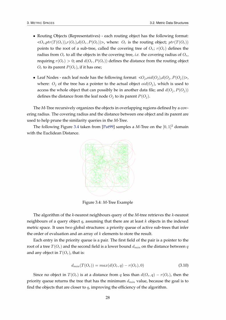
3. METRIC SPACES 3.2. Metric Data Structures
• Routing Objects (Representatives) - each routing object has the following format:<Or,ptr(T (Or)),r(Or),d(Or, P (Or))>, where: Or is the routing object; ptr(T (Or))
points to the root of a sub-tree, called the covering tree of Or; r(Or) defines theradius from Or to all the objects in the covering tree, i.e. the covering radius of Or,requiring r(Or) > 0; and d(Or, P (Or)) defines the distance from the routing objectOr to its parent P (Or), if it has one;
• Leaf Nodes - each leaf node has the following format: <Oj ,oid(Oj),d(Oj , P (Oj))>,where: Oj of the tree has a pointer to the actual object oid(Oj), which is used toaccess the whole object that can possibly be in another data file; and d(Oj , P (Oj))
defines the distance from the leaf node Oj to its parent P (Oj).
The M-Tree recursively organizes the objects in overlapping regions defined by a cov-ering radius. The covering radius and the distance between one object and its parent areused to help prune the similarity queries in the M-Tree.
The following Figure 3.4 taken from [Pat99] samples a M-Tree on the [0, 1]2 domainwith the Euclidean Distance.36 Chapter 4. The M-tree
Figure 4.3: A sample M-tree on the [0, 1]2 domain with the L2 distance.
nodes, i.e. d(Oi, P (Oi)) and r(Oi), is used to efficiently apply the triangle inequality
property.
4.2.1 Range Queries
According to Definition 2.4, the query range(Q, rQ, C) requests for all the database objectsOj, such that d(Oj, Q) ≤ rQ. Therefore, the algorithm RS (Range Search) has to follow
all such paths in the M-tree which cannot be excluded from leading to objects satisfying
the above inequality. Since the query threshold, rQ, does not change during the search
process, and provided the response set is required as a unit, the order with which nodes
are visited has no effect on the performance of RS algorithm. The RS algorithm is given
in Figure 4.5.
Figure 3.4: M-Tree Example
The algorithm of the k-nearest neighbours query of the M-tree retrieves the k-nearestneighbours of a query object q, assuming that there are at least k objects in the indexedmetric space. It uses two global structures: a priority queue of active sub-trees that inferthe order of evaluation and an array of k elements to store the result.
Each entry in the priority queue is a pair. The first field of the pair is a pointer to theroot of a tree T (Or) and the second field is a lower bound dmin on the distance between qand any object in T (Or), that is:
dmin(T (Or)) = max(d(Or, q)− r(Or), 0) (3.10)
Since no object in T (Or) is at a distance from q less than d(Or, q) − r(Or), then thepriority queue returns the tree that has the minimum dmin value, because the goal is tofind the objects that are closer to q, improving the efficiency of the algorithm.
28

3. METRIC SPACES 3.2. Metric Data Structures
Each entry of the nearest neighbours array has a pair where the first field denotesthe nearer object and the second field represents the distance from the object to q. Thealgorithm starts by filling the array with null objects with a infinite distance from q andthe idea is to compute for every sub-tree, an upper bound:
dmax(T (Or)) = d(Or, q) + r(Or) (3.11)
If between two sub-trees T (Or1) and T (Or2), the dmax of T (Or1) is smaller than thedmin of T (Or2), then the sub-tree T (Or2) can be pruned from the search and the dmaxvalues are inserted in the appropriate positions of the array.
When it reaches a leaf node Oj , it checks if the node fits in the array. If it does, it usesthe distance d(Oj , q) to discard active sub-trees in the queue that have a dmin bigger thand(Oj , q).
Until now, there are no publications about the remove operation [NUP11] in the M-Tree. So, regarding update operations, it only supports insertion.
The authors do not give theoretical results regarding the time complexities in theBig O Notation of the M-Tree, but experimental results with 10-nearest neighbours showsearch costs growing logarithmic with the number of objects [CPZ97].
3.2.3 DF-Tree
The DF-Tree (Distance Field Tree) is a paged, dynamic and generic secondary storagemetric data structure for indexing a finite metric space. It is based on the Slim-Tree[TTFS02] and improves it by tackling the compromise of having a representative of anode selected from the representatives of its children, allowing more representatives tobe used. On the other hand, the Slim-Tree is based on the M-Tree (3.2.2) and improvesit by tackling the compromise where the representatives restrict where a new object canbe stored, minimizing the intersection of nodes. The tree has the following structure(Figure 3.5) [TTFF02]:
Figure 1 - A DF-tree with node capacity=3,indexing 17 objects.
Figure 2 - Only objects in region 2are in the response set of the rangequery centered at sq with radius rq.
[10] [11]. An excellent survey on multidimensional access methodsis presented in [9]. However, all these methods were developedonly for vector data. On the other hand, many multimedia data donot have vectorial properties, but are in metric domains.
Previous work on metric access methods focused on the static case,for example: the structures proposed by Burkhard and Keller [5],Uhlmann [15], and also the vp-tree [16], GNAT [4] and mvp-tree[3], do not allows further insertions, deletions and updates after thetree creation. Overcoming this inconvenience, dynamic MAMstructures, including M-tree [7], Slim-tree [14] and the OMNI-family [12], have been developed.
The mvp-tree [3] and Omni-family [12] use multiple representativesto reduce the number of distance calculations performed duringqueries. In contrast to mvp-tree, the members of Omni-family aredynamic, allowing further insertions and deletions. However, theset of representatives used by the Omni-family is chosen during theearly construction phase of the tree and cannot be changedafterwards. The main idea is that, given a dataset S of objects in ametric domain, an object si S can be represented by its distancesto a set of global representatives, the foci. The HF algorithmpresented in [12] is used to choose these foci, among the objectsnear the border of the dataset. Yet, the authors show that theoptimum number of representatives is associated with the intrinsicdimensionality, ' , of the dataset, which is defined as the exponentin the power-law [8]:
n b r r( ) ∝
where is the average number of neighbors within distancenb r( )r or less from an arbitrary object, and stands for “is proportionalto”. We will use this result and the HF algorithm in this paper.
3. MOTIVATIONMetric trees store data in fixed-sized nodes, using reference objectsin each node to represent the other objects. Precalculated distancesbetween stored objects and the representatives are kept to speed upqueries on the tree. The triangular inequality property of metric do-mains allows pruning distance calculations, as explained following.
Let us first consider the objects sj S stored in a leaf node i. One ofthese objects, sRi, is chosen as the “representative” of node i. Thedistances between sRi and every object in this node are calculated,The largest one is defined as the covering radius rRi of that node.Therefore, any object farther than rRi from sRi cannot be found innode i. In the upper levels the same construct is employed, but the
entries are the representatives of their descendants and the coveringradius is: the distance between its representative and the farthestobject stored in the node, plus the covering radius of the nodewhere this object is the representative. Figure 1 shows a DF-treeindexing 17 objects, considering nodes with a maximum capacityof tree objects. Note that the root node does not have arepresentative and the dataset S is stored in the leafs. The globalrepresentatives are not depicted in this figure and will beintroduced later. All figures presented in this paper assumes adataset in a two-dimensional space with the Euclidean distancefunction, although the same concepts apply to any metric domain.
Now, consider a range queryof center sq and radius rq, asshown in figure 2. The querydefines tree regions: Region1 - objects that are fartherfrom sRep than its distance tothe query center sq, plus thequery radius rq; 2) Region 3- objects that are closer tosRep than its distance to thequery center sq, minus thequery radius rq; and Region2 - objects that do not satisfythe previous conditions.Thus, nodes that are com-pletely in Regions 1 or 3 can be pruned from the search process. Inthis way, every node i with representative sRi can be pruned if itsatisfy one of the following conditions:
a) d(sRep, sq)+rq < d(sRep, sRi)-rRi (Region 1) (Eq. 1)
b) d(sRep, sq)-rq > d(sRep, sRi)+rRi (Region 3) (Eq. 2)
The same pruning concept can be applied at leaf nodes, where thevalue of rRi is zero. Thus, the triangular inequality enables pruningboth on traversing of subtrees in non-leaf nodes and on distancecalculations from the query object to objects in the leaf nodes.
This mechanism leads to dynamic structures, because each newobject can be inserted in any of the nodes that are able to “cover”it. If no node covers it, the covering radius of an existing node isenlarged. If the node capacity is surpassed, the node splits and anew pair of representatives is chosen. When the root node splits,the tree grows one level. Thus, the construction of the tree occursin a bottom up approach, like the B-trees. Detailed algorithms toperform those operations can be found in [14] and [7].
Pruning can be enhanced by using more than one representative.In fact, the “amount of information” embodied in a simple relationbetween three objects (the query center, the target object sj and thenode representative) provided by the triangular inequality propertyis rather low, particularly in pure metric or in high-dimensionalspaces [2]. The combined use of two or more references eliminateslarger portions of the dataset. Figure 3 shows how much the regionwhere the candidate set of objects to answer the query shrinks byadding a global representative. If only the node representative isused for pruning, the shadowed region in figure 3(a) presents thevalid candidates to answer a range query with center object sq andradius rq. In figure 3(b) one Global Representative is also used andthe darker shadowed (smaller) region indicates where thecandidates could be for the same range query of (a).
A
A
A
A
B
B
B
B
C
C
C
C
D
D
D
E
E
E
F
F
F
G
G
H
H
I
I
J
J
K
K
L
L
M
M
N
N
O
O
P
PQ
Q
Gro
win
g di
rect
ion
Root
Index Nodes
Leaf Nodes
220
(a) Regions Figure 1 - A DF-tree with node capacity=3,indexing 17 objects.
Figure 2 - Only objects in region 2are in the response set of the rangequery centered at sq with radius rq.
[10] [11]. An excellent survey on multidimensional access methodsis presented in [9]. However, all these methods were developedonly for vector data. On the other hand, many multimedia data donot have vectorial properties, but are in metric domains.
Previous work on metric access methods focused on the static case,for example: the structures proposed by Burkhard and Keller [5],Uhlmann [15], and also the vp-tree [16], GNAT [4] and mvp-tree[3], do not allows further insertions, deletions and updates after thetree creation. Overcoming this inconvenience, dynamic MAMstructures, including M-tree [7], Slim-tree [14] and the OMNI-family [12], have been developed.
The mvp-tree [3] and Omni-family [12] use multiple representativesto reduce the number of distance calculations performed duringqueries. In contrast to mvp-tree, the members of Omni-family aredynamic, allowing further insertions and deletions. However, theset of representatives used by the Omni-family is chosen during theearly construction phase of the tree and cannot be changedafterwards. The main idea is that, given a dataset S of objects in ametric domain, an object si S can be represented by its distancesto a set of global representatives, the foci. The HF algorithmpresented in [12] is used to choose these foci, among the objectsnear the border of the dataset. Yet, the authors show that theoptimum number of representatives is associated with the intrinsicdimensionality, ' , of the dataset, which is defined as the exponentin the power-law [8]:
n b r r( ) ∝
where is the average number of neighbors within distancenb r( )r or less from an arbitrary object, and stands for “is proportionalto”. We will use this result and the HF algorithm in this paper.
3. MOTIVATIONMetric trees store data in fixed-sized nodes, using reference objectsin each node to represent the other objects. Precalculated distancesbetween stored objects and the representatives are kept to speed upqueries on the tree. The triangular inequality property of metric do-mains allows pruning distance calculations, as explained following.
Let us first consider the objects sj S stored in a leaf node i. One ofthese objects, sRi, is chosen as the “representative” of node i. Thedistances between sRi and every object in this node are calculated,The largest one is defined as the covering radius rRi of that node.Therefore, any object farther than rRi from sRi cannot be found innode i. In the upper levels the same construct is employed, but the
entries are the representatives of their descendants and the coveringradius is: the distance between its representative and the farthestobject stored in the node, plus the covering radius of the nodewhere this object is the representative. Figure 1 shows a DF-treeindexing 17 objects, considering nodes with a maximum capacityof tree objects. Note that the root node does not have arepresentative and the dataset S is stored in the leafs. The globalrepresentatives are not depicted in this figure and will beintroduced later. All figures presented in this paper assumes adataset in a two-dimensional space with the Euclidean distancefunction, although the same concepts apply to any metric domain.
Now, consider a range queryof center sq and radius rq, asshown in figure 2. The querydefines tree regions: Region1 - objects that are fartherfrom sRep than its distance tothe query center sq, plus thequery radius rq; 2) Region 3- objects that are closer tosRep than its distance to thequery center sq, minus thequery radius rq; and Region2 - objects that do not satisfythe previous conditions.Thus, nodes that are com-pletely in Regions 1 or 3 can be pruned from the search process. Inthis way, every node i with representative sRi can be pruned if itsatisfy one of the following conditions:
a) d(sRep, sq)+rq < d(sRep, sRi)-rRi (Region 1) (Eq. 1)
b) d(sRep, sq)-rq > d(sRep, sRi)+rRi (Region 3) (Eq. 2)
The same pruning concept can be applied at leaf nodes, where thevalue of rRi is zero. Thus, the triangular inequality enables pruningboth on traversing of subtrees in non-leaf nodes and on distancecalculations from the query object to objects in the leaf nodes.
This mechanism leads to dynamic structures, because each newobject can be inserted in any of the nodes that are able to “cover”it. If no node covers it, the covering radius of an existing node isenlarged. If the node capacity is surpassed, the node splits and anew pair of representatives is chosen. When the root node splits,the tree grows one level. Thus, the construction of the tree occursin a bottom up approach, like the B-trees. Detailed algorithms toperform those operations can be found in [14] and [7].
Pruning can be enhanced by using more than one representative.In fact, the “amount of information” embodied in a simple relationbetween three objects (the query center, the target object sj and thenode representative) provided by the triangular inequality propertyis rather low, particularly in pure metric or in high-dimensionalspaces [2]. The combined use of two or more references eliminateslarger portions of the dataset. Figure 3 shows how much the regionwhere the candidate set of objects to answer the query shrinks byadding a global representative. If only the node representative isused for pruning, the shadowed region in figure 3(a) presents thevalid candidates to answer a range query with center object sq andradius rq. In figure 3(b) one Global Representative is also used andthe darker shadowed (smaller) region indicates where thecandidates could be for the same range query of (a).
A
A
A
A
B
B
B
B
C
C
C
C
D
D
D
E
E
E
F
F
F
G
G
H
H
I
I
J
J
K
K
L
L
M
M
N
N
O
O
P
PQ
Q
Gro
win
g di
rect
ion
Root
Index Nodes
Leaf Nodes
220
(b) Tree
Figure 3.5: DF-Tree Example
• Internal Node - each node entry has the following format: <Si, Ri, d(Si, SRi), Dfi,Ptr(TSi), NEntries(Ptr(TSi))>, where: Si is the representative object of the re-spective sub-tree pointed by Ptr(TSi); Ri is the covering radius of the sub-tree;
29

3. METRIC SPACES 3.2. Metric Data Structures
d(Si, SRi) is the distance between Si and the representative of this node SRi; Dfi isthe distance fields, i.e. the distance between the representative object and the globalrepresentative i; and NEntries(Ptr(TSi)) is the current number of entries in thesub-tree;
• Leaf Node - each leaf node has the following format: <Si, Oidi, Dfi, d(Si, SRi)>,where: Si is the actual object and its respective object identifier Oidi; Dfi is thedistance fields between the object and the global representative i; and d(Si, SRi) isthe distance between Si and the representative of this node SRi.
The basic idea behind the DF-Tree is to build the tree combining the use of one rep-resentative per node (e.g. in the Slim-Tree) with the distance fields generated by eachglobal representative. A global representative is chosen from the objects in the tree andis independent from the other representatives, including node representatives, and is ap-plied to each object in the tree. The goal of using global representatives is to prune evenmore the number of distance evaluations. The number of distance evaluations that canbe pruned depends on the areas defined by each representative object (Figure 3.6a, takenfrom [TTFF02]). Using the global representatives, this number can be pruned even more(Figure 3.6b).
Objects not prunned (20 objects)
Objects not prunned (4 objects)
Response set (2 objects)
Response set (2 objects)
RqSq
Srep
Global
representative
(a) Without
Objects not prunned (20 objects)
Objects not prunned (4 objects)
Response set (2 objects)
Response set (2 objects)
RqSq
Srep
Global
representative
(b) With
Figure 3.6: DF-Tree Pruning using Global Representative
The number and placement of global representatives, unlike node representatives thatare defined during the tree construction and, therefore, cannot be changed, can be calcu-lated and modified when the first similarity query is answered or after the tree building.Given a dimensionality dim, the number of global representatives can be only ddime. TheDF-Tree has a method that evaluates if it currently needs to update its set of global rep-resentatives, so the set is not inadequate and does not compromise the pruning ability ofthe tree. If the tree needs to update its global representatives, there is also a method forthis purpose.
As the DF-Tree is a descendent of the M-Tree, its algorithm for the k-nearest neigh-bours query is similar to the algorithm of the M-Tree.
30

4Approach
This chapter explains how metric data structures help solving the problem and presentsthe architecture of the solution, justifying some choices made. Then, the primary storagesolution is detailed and has its time complexity evaluated. By the end of this chapter, thesecondary memory solution is also explained.
4.1 Introduction
4.1.1 Implementing the SNN using Metric Data Structures
Implementing the SNN with metric data structures, helps to solve the issues stated in 1.2:
• Storage - If we are handling with a big spatial data set that does not fit into primarystorage, then it is necessary that the metric data structure chosen is stored in sec-ondary storage. This is an important matter because, if the metric data structureis stored in secondary storage, the storage access times must be accounted to theruntime of the SNN. Therefore, the SNN should deal with both of these situations,handling a metric data structure in primary or secondary storage;
• Fine-tuning of Parameters - The attempts carried out to find the right parametersthat give output to the best possible clustering results for a given data set, lead tomultiple runs of the SNN.
As stated before, the time complexity of the SNN in the worst case is O(n2). Thisquadratic behaviour is observed experimentally in chapter 5 with a referenced im-plementation of the Original SNN. The key factor for this time complexity is the
31

4. APPROACH 4.1. Introduction
k-nearest neighbours queries for each object in a data set, since one single query isevaluated in the worst case with a time complexity of O(n).
With these requirements, running the Original SNN multiple times can be timeconsuming. So, in [ESK03], metric data structures are briefly suggested to reducethe time complexity of the SNN. With such an improvement, running the OriginalSNN multiple times would become faster and less time consuming.
With the integration of metric data structures with the Original SNN, it is convenientto consider three types of runs (Figure 4.1): Tree, Neighbouring and Clustering (TNC) -the initial run, where it is necessary to build the metric data structure, query and storethe k-nearest neighbours of each object, before carrying out the clustering steps of theSNN; Neighbouring and Clustering (-NC) - the run where the metric data structure isalready built, but it still needs to query and store the k-nearest neighbours, before theclustering steps of the SNN; and Clustering (–C) - the run where the metric data structureis already built and the k-nearest neighbours are already known, for example, the k ofthe new run is less than or equal to the k of the previous run. As the k is less than orequal to the k previously calculated, the SNN can compute its clustering steps withoutquerying the metric data structure again, only using part or all of the previously acquiredk-nearest neighbours, requiring the k-nearest neighbours to be ordered ascendantly bytheir distances from the queried object.
Start
End
Build Metric Data Structure
Read k
Get k-Nearest
Neighbours
SNN Algorithm
Next Iteration
Is New k > Prev.
k
Yes
No
No
Yes Read
k
--C
-NC
TNC
Figure 4.1: Runs Taxonomy
32

4. APPROACH 4.1. Introduction
4.1.2 Architecture
The first step taken towards the architecture consisted on choosing which metric datastructures to use with the SNN. As mentioned on chapter 3, the chosen metric data struc-tures, for each type of storage, were: the kd-Tree and the DF-Tree. The kd-Tree for beingpopular in the literature [CNBYM01], for being written for primary storage in variousprogramming languages, for having its time complexity evaluated in the Big O Notationand for being suited for low dimensionality problems (e.g. spatial data) [Mar06]. TheDF-Tree because, there are few alternatives of secondary storage metric data structuresand it delivers better results [TTFF02].
The next choice was in which programming language write the SNN. Since the kd-Tree is written in a wide range of programming languages, this metric data structure wasnot a bottleneck in the final verdict. On the other hand, as the DF-Tree is only written inC++ (part of the GBDI Arboretum library in [Dat06]), at first this was the primary choice.Nevertheless, because of Weka [HFH+09] being written in Java, because of having moreknowledge and practice in Java and because of having found a kd-Tree in Java [Sav12],well-structured and well-documented, the SNN was written in Java.
Writing the SNN in Java, brought up an issue regarding how the SNN would get ac-cess to the k-nearest neighbours given by the DF-Tree, since the DF-Tree is only writtenin C++. The Java Native Interface (JNI) [Lia99] and the Protocol Buffers [Goo12] wereconsidered. However, as JNI should only be used when there are no other alternativesolutions that are more appropriate, since applications that use the JNI have inherent dis-advantages [Lia99] and as Protocol Buffers seemed more risky at the time, representinga bumpier road, these two options were discarded. Therefore, the found solution was touse a DataBase Management System (DBMS) as a mean of connection between the SNNin Java and the DF-Tree in C++, without neglecting the access times that are demanded bythe use of a DBMS. In the following experimental results, the MySQL DBMS was chosenwith no particular reason, as every DMBS can be used.
In order to do this, when using the DF-Tree, it is deployed a Structured Query Lan-guage (SQL) file with all the attributes that define each object in a data set and their re-spective k-nearest neighbours, using identifiers for each object (explained in more detailin section 4.3.1). With this, the SNN implementation only works with identifiers dur-ing the clustering and does not need to store in primary storage the whole objects, sincethey are stored in secondary storage, requiring less primary storage space. When usingthe kd-Tree, the objects stay in the primary storage metric data structure, while the SNNcontinues to cluster with support to their identifiers.
Considering all the above decisions, the solution was designed according to the ar-chitecture in figure 4.2. There are two different modules:
• Primary Storage Module - represented by the left side of the figure. Everythingworks in primary storage and is written in Java. While using the Reader, it startsby reading each object from the data set, preprocessing it and giving to each object
33

4. APPROACH 4.1. Introduction
C++ Reader DF-Tree
Wrapper
kd-Tree
Wrapper Database
3. Get k-Nearest Neighbours
6. Get Objects
5. Get k-Nearest Neighbours
8. Get Objects
4. k-Nearest Neighbours
6. k-Nearest Neighbours
5. Clustering Results
7. Clustering Results
4. Get and Import the SQL File
2. Put Objects
2. Put Objects
3. Get k-Nearest Neighbours
Data Set
Data Set
DB Output
DB Reader
Output
Reader
SNN
Secondary Storage Primary Storage
1. Read Objects
1. Read Objects
Figure 4.2: Architecture
an unique identifier, in order to store each object in the kd-Tree, using its respectivewrapper. All the remaining components work with identifiers. Afterwards, theReader gets the k-nearest neighbours of each object and gives them to the SNN,triggering the clustering process. When the SNN ends the clustering, the Outputuses the identifiers of the objects to get their attributes from the kd-Tree, using alsoits respective wrapper, in order to generate a readable output file with the clusteringresults sent by the SNN.
• Secondary Storage Module - represented by the right side of the figure. The C++Reader and the DF-Tree (the actual metric data structure and its wrapper) are writ-ten in C++. All other components are written in Java, working in primary storage.As the primary storage module, the secondary storage module begins by using theC++ Reader to read each object from the data set, preprocessing it and giving to eachobject an unique identifier, storing each object in the DF-Tree, using its respectivewrapper. Then, the C++ Reader obtains the k-nearest neighbours from the DF-Treeand creates an SQL file to be imported to a DBMS with all objects and respectivek-nearest neighbours. From this point forward, the DB Reader accesses the DBMS,in order to obtain the k-nearest neighbours and gives them to the SNN to start theclustering process. When the clustering is achieved, the DB Output uses the iden-tifiers of each object to query the DBMS for the attributes of each of the objects,creating also a readable output file with the clustering results sent by the SNN.
34

4. APPROACH 4.2. Using the kd-Tree with the SNN
Both modules use wrappers in the metric data structures to create a level of trans-parency to the Readers or the Outputs, so they do not need to be changed, when used witha different metric data structures. Each of these two modules are explained in more detailin the following sections.
4.2 Using the kd-Tree with the SNN
On this section, this approach is explained and the improvement that can be obtained byusing the kd-Tree with the SNN is evaluated, regarding its time complexity, by makingthe k-nearest neighbours queries more efficient. The main procedure written for thisapproach is summed up in Algorithm 1. This approach will be known in this documentby kd-SNN.
Algorithm 1 Primary Storage Procedure
1: function kD-SNN2: while making consecutive runs do3: if first run then4: use the Reader to build the kd-Tree with the objects in a data set5: end if6: if first run or new k > previous k then7: use the Reader to obtain the k-nearest neighbours8: end if9: SNN(k-nearest neighbours)
10: if output is requested then11: use the Output12: end if13: end while14: end function
4.2.1 Reader
As disclosed in the architecture, the Reader is used to read a data set and build the kd-Treewith all objects, in order to obtain the k-nearest neighbours of each object. Each Readeris written for a specific format of a data set and, when a new Reader needs to be written,it has to follow an appropriate interface with the required methods to read the data set,build the tree and query for the k-nearest neighbours of each object.
On the first run of the algorithm (TNC), the kd-Tree needs to be built with a data set.The time complexity in the average case of building the kd-Tree with low dimensionalityobjects is O(d × n × log n) [FBF77], where d is the dimensionality of a data set. This lowdimensionality scenario is often witnessed when dealing with spatial data, even whenthe distance function used is not simply the geographical distance between objects. Forinstance, in [SSMPW12], it is used a distance function that, besides using the geographiclocation, also uses the bearing (heading) of a given motion vector, to measure the distance
35

4. APPROACH 4.2. Using the kd-Tree with the SNN
between objects. Under these circumstances, it can be asserted that the time complexityin the average case of building the kd-Tree is proportional to O(n× log n).
Once the kd-Tree is built, the next step is to query it for the k-nearest neighbours ofeach object. The resulting k-nearest neighbours and their respective distances are storedin a Hash Map that requires the sets of k-nearest neighbours to be ordered ascendantlyby the distance between objects. The time complexity in the average case of one singlek-nearest neighbours query is proportional toO(log n), where the constant of proportion-ality depends on the distance function, on the dimensionality of a data set and on thek value. Therefore, the time complexity in the average case of obtaining the k-nearestneighbours of all objects in a data set is also proportional to O(n× log n).
After obtaining the k-nearest neighbours of each object, they are provided to the SNN,triggering the beginning of the clustering.
4.2.2 SNN
The SNN implemented was based on the representative objects-based approach explainedin section 2.2.3 and has several clustering steps as in Algorithm 2.
Algorithm 2 Procedure of the SNN
Require: A Hash Map with the k-nearest Neighbours of each Object1: function SNN2: MEASURING THE SIMILARITIES AND THE DENSITIES
3: NOISE DETECTION
4: CLUSTERING THE REPRESENTATIVE OBJECTS
5: CLUSTERING THE REMAINING OBJECTS
6: CLUSTERING THE NOT YET CLUSTERED OBJECTS
7: end function
As soon as the SNN obtains the k-nearest neighbours of each object, it initiates theclustering process, starting by measuring the similarity between objects and their respec-tive densities (Algorithm 3). The most complex step is to compute the similarity betweena pair of objects, since the SNN intersects their sets of k-nearest neighbours to determinethe number of shared nearest neighbours. This intersection has a time complexity in theworst case evaluated in O(k2), corresponding to going over one of the sets of k-nearestneighbours for every nearest neighbour in another set. The calculated similarities be-tween mutual neighbours should be stored in a Hash Map, so they can be reused inthe following steps of the SNN, avoiding the time complexity of recalculating the sim-ilarities. Since, the SNN needs to iterate over all objects, intersecting a set of k-nearestneighbours of an object with the set of k-nearest neighbours of each of its neighbours,which as asserted before has a time complexity of O(k2), algorithm 3 is evaluated with atime complexity in the worst case of O(n× k × k2) ⇐⇒ O(n× k3).
Now that the density of each object is known, the noise must be detected (Algorithm4). This algorithm initially requires all objects to be defined as noise. It starts by iterating
36
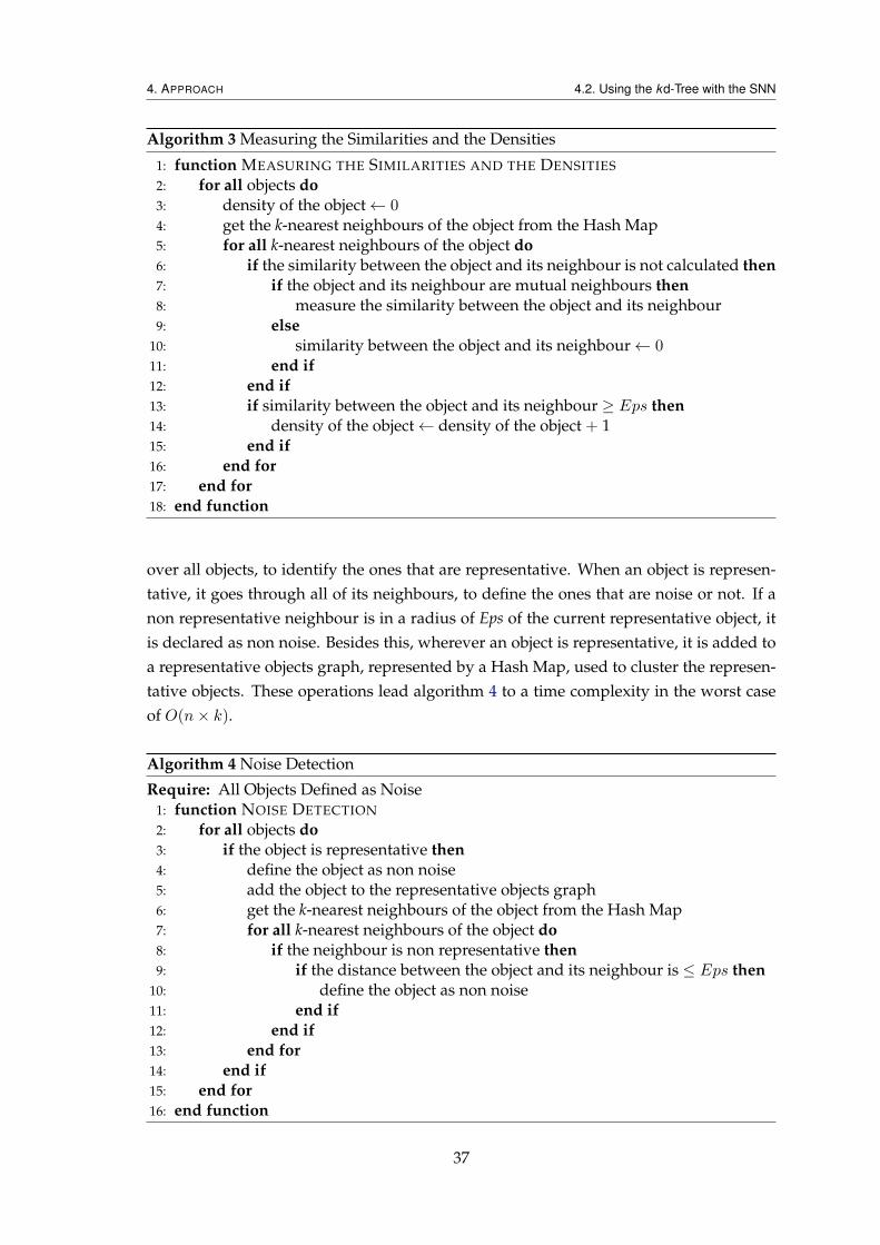
4. APPROACH 4.2. Using the kd-Tree with the SNN
Algorithm 3 Measuring the Similarities and the Densities
1: function MEASURING THE SIMILARITIES AND THE DENSITIES
2: for all objects do3: density of the object← 04: get the k-nearest neighbours of the object from the Hash Map5: for all k-nearest neighbours of the object do6: if the similarity between the object and its neighbour is not calculated then7: if the object and its neighbour are mutual neighbours then8: measure the similarity between the object and its neighbour9: else
10: similarity between the object and its neighbour← 011: end if12: end if13: if similarity between the object and its neighbour ≥ Eps then14: density of the object← density of the object + 115: end if16: end for17: end for18: end function
over all objects, to identify the ones that are representative. When an object is represen-tative, it goes through all of its neighbours, to define the ones that are noise or not. If anon representative neighbour is in a radius of Eps of the current representative object, itis declared as non noise. Besides this, wherever an object is representative, it is added toa representative objects graph, represented by a Hash Map, used to cluster the represen-tative objects. These operations lead algorithm 4 to a time complexity in the worst caseof O(n× k).
Algorithm 4 Noise Detection
Require: All Objects Defined as Noise1: function NOISE DETECTION
2: for all objects do3: if the object is representative then4: define the object as non noise5: add the object to the representative objects graph6: get the k-nearest neighbours of the object from the Hash Map7: for all k-nearest neighbours of the object do8: if the neighbour is non representative then9: if the distance between the object and its neighbour is ≤ Eps then
10: define the object as non noise11: end if12: end if13: end for14: end if15: end for16: end function
37

4. APPROACH 4.2. Using the kd-Tree with the SNN
Afterwards, the clustering is initiated, starting with the representative objects, thenthe remaining objects (non representative and non noise) and ending with the not yetclustered objects (Algorithm 2).
Algorithm 5 Clustering the Representative Objects
1: function CLUSTERING THE REPRESENTATIVE OBJECTS
2: for all objects do3: if the object is representative then4: get the k-nearest neighbours of the object from the Hash Map5: for all k-nearest neighbours of the object do6: if the neighbour is representative then7: if the similarity between the object and its neighbour is ≥ Eps then8: connect the object and its neighbour in the graph9: end if
10: end if11: end for12: end if13: end for14: identify the clusters obtained by finding the connected sub-graphs in the graph15: end function
The most important algorithm is the clustering of the representative objects, since itdefines the backbone of the clusters (Algorithm 5). For that, the SNN iterates over allobjects, connecting in the graph all representative objects and respective representativek-nearest neighbours that have a similarity greater than Eps. Connecting the objects takesthe time complexity of checking if the connection already exists. Since, each object as atmost k connections, connecting a pair requires a O(k) time complexity in the worst case,leading this step to a time complexity in the worst case ofO
(n×k×O(k)
)⇐⇒ O(n×k2).
After iterating all and connecting the possible objects, the SNN finds all maximallyconnected components [Lov04] of the graph, that represent the clusters, using the breadthfirst search. The breadth first search has a time complexity in the worst case of O(V +A)
[WCC09], where V represents the number of vertices in the graph and A the number ofarcs (connections) in the graph. Since, in this case, the number of vertices is at most thenumber of objects and the number of connections is at most the number of objects timesthe number of k-nearest neighbours, finding all maximally connected components of thegraph takes in the worst case O
(n+ (n× k)
)⇐⇒ O(n× k).
So, algorithm 5 has a time complexity in the worst case of O(n× k2).After obtaining the backbone of the clusters, all remaining objects are clustered to the
cluster of the representative object with which they are more similar (Algorithm 6).In order to find the most similar representative object, the Eps threshold is not used to
break connections between mutual neighbours. The idea is to cluster the the non repre-sentative and non noise objects to a cluster of a representative neighbour with which it isa mutual neighbour and shares the highest similarity possible among its representativeneighbours, even if the highest similarity is zero and they are just connected, because
38

4. APPROACH 4.2. Using the kd-Tree with the SNN
Algorithm 6 Clustering the Remaining Objects
1: function CLUSTERING THE REMAINING OBJECTS
2: for all objects do3: if the object is non representative and non noise then4: get the k-nearest neighbours of the object from the Hash Map5: for all k-nearest neighbours of the object do6: if the neighbour is representative then7: check if this is the most similar representative neighbour8: end if9: end for
10: if found a most similar representative neighbour then11: the object joins the cluster of the neighbour12: else13: find the predominant cluster between its neighbours14: if found a predominant cluster between its neighbours then15: the object joins the predominant cluster16: else17: define the object as not yet clustered18: end if19: end if20: end if21: end for22: end function
both objects are mutual neighbours.
In case they do not have a representative object as a neighbour, their neighbours areevaluated, with the goal of finding a predominant cluster between them. The predomi-nant cluster step was introduced in this implementation with the purpose of giving theremaining objects, that do not have a representative object as their neighbour, a cluster.In order to do this, all the neighbours of a non representative object are evaluated and themost common cluster between them is chosen as the predominant cluster. However, asthe clustering of the remaining objects might not yet be completed, while the neighboursare being checked for a predominant cluster, some might not have a predominant clusteramong its neighbours, because some of these neighbours might be remaining objects tooand were not processed yet. Objects in this situation are defined as not yet clustered andwill be clustered in the next step of the SNN.
Finding the predominant cluster among the neighbours has a time complexity in theworst case that depends on two operations: the clustering scoring, in order to identify themost predominant cluster, which has a time complexity in the worst case ofO(k); and thelooking over all the scored clusters, for the one with the most occurrences, which has atime complexity of O(k) in the worst case. Therefore, finding the predominant clusterhas a time complexity in the worst case of O
(O(k) +O(k)
)⇐⇒ O(k).
This way, for each remaining object, either a representative object is found among itsneighbours, or the predominant cluster among its neighbours needs to be found, bringing
39

4. APPROACH 4.2. Using the kd-Tree with the SNN
the time complexity in the worst case of algorithm 6 to O(n× (k+O(k)
)⇐⇒ O(n× k).
The last algorithm gives all not yet clustered objects, one last chance of being clusteredby being clustered to the predominant cluster among its k-nearest neighbours (Algorithm7).
Algorithm 7 Clustering the Not Yet Clustered Objects
1: function CLUSTERING THE NOT YET CLUSTERED OBJECTS
2: for all not yet clustered objects do3: find the predominant cluster between its neighbours4: if found a predominant cluster between its neighbours then5: the object joins the predominant cluster6: else7: define the object as noise8: end if9: end for
10: end function
As pointed out in the previous algorithm (Algorithm 6), the time complexity in theworst case of finding the predominant cluster among the k-nearest neighbours of an ob-ject isO(k). Since, all not yet clustered objects need to be iterated and for each one findingits predominant cluster, algorithm 7 has a time complexity in the worst case of O(m× k),where m denotes the number of not yet clustered objects, that were not clustered in theprevious algorithms of the SNN.
Algorithms Worst Case
Measuring the Similarities and the Densities O(n× k3)Noise Detection O(n× k)
Clustering the Representative Objects O(n× k2)Clustering the Remaining Objects O(n× k)
Clustering the Not Yet Clustered Objects O(m× k)
Figure 4.3: Time Complexities of the Algorithms of the SNN
Considering all the time complexities evaluated (Figure 4.3), it follows that the timecomplexity in the worst case of the clustering steps of the SNN is O(n × k3), which isproportional to O(n).
4.2.3 Output
The Output is optional and can be done in various formats, they just need to be writtenaccording to an available interface, not restricting the user to some formats. Nevertheless,two types of outputs were implemented, since Weka was used as a plot tool: the formatof an Attribute-Relation File Format (ARFF) file supported by Weka or plotted on a chartalso with support to Weka.
40

4. APPROACH 4.2. Using the kd-Tree with the SNN
An ARFF file is a standard way of representing data sets that consist of indepen-dent, unordered instances of objects and does not involve relationships between instances[WF05].
%Example of an ARFF file@relation arff_example
@attribute X numeric@attribute Y numeric@attribute cluster {1, 2, 3}
@data-8.667331, 41.149643, 1-8.66603, 41.153057, 1-8.663754, 41.146879, 1-8.579538, 41.201668, 2-8.659527, 41.150455, 1-8.57466, 41.192401, 2-8.575636, 41.198254, 2-8.582302, 41.182484, 2-8.630425, 41.146716, 3-8.627662, 41.146554, 3-8.579863, 41.191588, 2-8.585716, 41.185735, 2
Figure 4.4: Example of an ARFF file
Figure 4.4 is an example of an ARFF file, where % represent the comments. Followingthe comments, there is the name of the data set (@relation) and, the attributes used in thedata set are defined (@attribute), in this case, X, Y and cluster. Nominal attributes are de-fined also by the set of values that they can take, for example, cluster. Numeric values arefollowed by the keyword numeric. After the attributes definitions, i.e. following the @dataline, the objects are finally represented, one by each line. The values of each attribute ofthe object are separated by commas. Although the cluster attribute is the predicted value,in an ARFF file there is no reference to what attribute is the class attribute.
Since the SNN only uses identifiers, the clustering results are also presented withidentifiers. So, in order to give an appropriate output and getting all the informationneeded for the output format, it is required to get the attributes of the objects. In order todo this, the Reader must provide access to an iterator to the kd-Tree, giving access to allthe attributes of the objects.
4.2.4 Time Complexity Evaluation
Bearing in mind that besides the above clustering steps required by the SNN it is alsoneeded to index the metric data structure and get the k-nearest neighbours of each objectin the data set, it follows that the time complexity of the kd-SNN depends solely on thetime complexity of building the kd-Tree, of the k-nearest neighbours queries done to thekd-Tree and of the clustering steps of the SNN. Since the kd-Tree is built in a O(n× log n)
time complexity in the average case and is queried for the k-nearest neighbours of each
41
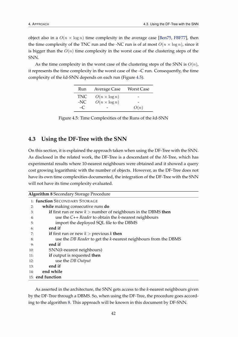
4. APPROACH 4.3. Using the DF-Tree with the SNN
object also in a O(n × log n) time complexity in the average case [Ben75, FBF77], thenthe time complexity of the TNC run and the -NC run is of at most O(n × log n), since itis bigger than the O(n) time complexity in the worst case of the clustering steps of theSNN.
As the time complexity in the worst case of the clustering steps of the SNN is O(n),it represents the time complexity in the worst case of the –C run. Consequently, the timecomplexity of the kd-SNN depends on each run (Figure 4.5).
Run Average Case Worst Case
TNC O(n× log n) --NC O(n× log n) -–C - O(n)
Figure 4.5: Time Complexities of the Runs of the kd-SNN
4.3 Using the DF-Tree with the SNN
On this section, it is explained the approach taken when using the DF-Tree with the SNN.As disclosed in the related work, the DF-Tree is a descendant of the M-Tree, which hasexperimental results where 10-nearest neighbours were obtained and it showed a querycost growing logarithmic with the number of objects. However, as the DF-Tree does nothave its own time complexities documented, the integration of the DF-Tree with the SNNwill not have its time complexity evaluated.
Algorithm 8 Secondary Storage Procedure
1: function SECONDARY STORAGE
2: while making consecutive runs do3: if first run or new k > number of neighbours in the DBMS then4: use the C++ Reader to obtain the k-nearest neighbours5: import the deployed SQL file to the DBMS6: end if7: if first run or new k > previous k then8: use the DB Reader to get the k-nearest neighbours from the DBMS9: end if
10: SNN(k-nearest neighbours)11: if output is requested then12: use the DB Output13: end if14: end while15: end function
As asserted in the architecture, the SNN gets access to the k-nearest neighbours givenby the DF-Tree through a DBMS. So, when using the DF-Tree, the procedure goes accord-ing to the algorithm 8. This approach will be known in this document by DF-SNN.
42

4. APPROACH 4.3. Using the DF-Tree with the SNN
4.3.1 C++ Reader
The C++ Reader is in charge of building the DF-Tree with a data set, of querying it for thek-nearest neighbours and of deploying a SQL file with all the attributes that define theobjects and their respective k-nearest neighbours.
Although it is possible to reuse several methods written, for instance, the one thatgives the output in the format of a SQL file, for each format of a data set, a C++ Readerhas to be written, as in the primary storage approach with the kd-Tree.
Since the DF-Tree works in secondary storage, the DF-Tree is stored in a DAT filewith a specific format created by the authors of the DF-Tree, resorting to serialize anddeserialize methods written specifically for the type of objects in a data set.
After the DF-Tree is built, it becomes capable of answering the k-nearest neighboursqueries. The results are then given in the format of a SQL file that creates two tables withthe following format:
• Objects Table - each row consists of the identifier (ID) of an object and all the at-tributes that define the respective object in a data set;
ID . . .
0 . . ....
...n− 1 . . .
Figure 4.6: SQL File - Objects Table
• k-Nearest Neighbours Table - each row represents the identifier of an object, theidentifier of one of its k-nearest neighbours and the distance between them. Thisrow is repeated k times for each object.
ID k-Nearest Neighbour ID Distance
0 . . . . . ....
. . ....
n− 1 . . . . . .
Figure 4.7: SQL File - k-Nearest Neighbours Table
4.3.2 DB Reader
After acquiring the SQL file from the C++ Reader, it is imported to a DBMS, so the SNNcan gain access to the k-nearest neighbours.
The DB Reader was created for this purpose and is generic for any format of a data set,since its goal is just to read the standard k-nearest neighbours table stored in a DBMS, as
43
4. APPROACH 4.3. Using the DF-Tree with the SNN
it is the same for all data sets. In order to do this, it requires a DBMS connection interfacewritten in Java for the DBMS.
When the k-nearest neighbours are all in primary storage, the SNN can start its clus-tering progress. Bear in mind that, since the k value is limited to the number of neigh-bours stored in the DBMS, if there is a need to use more k-nearest neighbours than theones stored in the DBMS, then the C++ Reader has to be run again, to get the SQL file withall the new sets of k-nearest neighbours.
Due to technical difficulties with the use of the DF-Tree, every time the C++ Readeris run again, the tree needs to be built and cannot be reused between runs. So, in thecontext of the C++ Reader, every time it is run, it matches the TNC run, since the -NC rundoes not exit. However, in the primary storage component, the -NC run exists, since wecan query the DBMS for more neighbours than we initially had requested, as long as thenumber of neighbours does not surpass the number of neighbours stored in the DBMS.If we do not need to query for more neighbours, either the C++ Reader or the DBMS, therun –C is executed.
The SNN used in the DF-SNN is the same presented in section 4.2.2, because there is acare to read the k-nearest neighbours in the format required by the SNN written, fosteringthe portability of the SNN.
4.3.3 DB Output
As the SNN ends its clustering and produces the respective clustering results, the outputmay be given via the DB Output. The difference between the DB Output and the Output,is the source of information. As the Output in the kd-SNN uses the identifiers to make thematch with the objects given by the iterator, the DF-SNN uses the identifiers to get theinformation directly from the DBMS. Everything else is exactly the same, the DB Reader iswritten to give output in an ARFF file or plotted on a chart with support to Weka. Othertypes of output are also supported, they just need to be written according to an interfaceavailable.
The DB Output requires, as the DB Reader, a connection to the DBMS used by theDF-SNN.
44

5Experimental Results
This chapters discloses the experimental results, where three synthetic data sets and onereal data set, entitled Marin Data, were used, in order to evaluate the quality of the clus-tering results obtained with the kd-SNN and with the DF-SNN. Each of these results iscompared with the ones obtained with another implementation of a variant of the SNN.Another real data set, extracted from Twitter, was used to evaluate the scalability of thekd-SNN and of the DF-SNN. Their scalability is also compared with the scalability of areferenced implementation of the Original SNN.
5.1 Data Sets
5.1.1 Synthetic
Three synthetic data sets were used, each of them has objects defined by two attributesthat represent the objects position in a two-dimensional space (Figure 5.1). The dis-tance between the objects is measured with the generic euclidean distance over a two-dimensional space.
Attribute Type
X Decimal NumberY Decimal Number
Figure 5.1: Attributes of the Synthetic Data Sets
These three datasets were chosen due to their usage in the literature and because twoof them were used in experimental results to validate the representative objects-based
45

5. EXPERIMENTAL RESULTS 5.1. Data Sets
approach of the SNN [MSC05], serving as benchmark.
As can be seen in figure 5.2, each data set has a unique and specific clustering ten-dency, where the main clusters can be easily perceived by visually analysing the distri-bution of the objects in the data set.
41.13
41.14
41.15
41.16
41.17
41.18
41.19
41.2
41.21
41.22
−8.7 −8.68 −8.66 −8.64 −8.62 −8.6 −8.58 −8.56
Y
X
(a) Synthetic 1
41.19
41.195
41.2
41.205
41.21
41.215
41.22
41.225
−8.675 −8.67 −8.665 −8.66 −8.655 −8.65 −8.645 −8.64 −8.635 −8.63
Y
X
(b) Synthetic 2
41.196
41.198
41.2
41.202
41.204
41.206
41.208
41.21
41.212
41.214
41.216
−8.675 −8.67 −8.665 −8.66 −8.655 −8.65 −8.645 −8.64 −8.635
Y
X
(c) Synthetic 3
Figure 5.2: Distribution of the Synthetic Data Sets
The first synthetic data set (Figure 5.2a) has 322 objects, the second (Figure 5.2b) has292 objects and the third and last (Figure 5.2c) has 523 objects. Some of these objectsclearly represent noise, as can be seen in the data sets respective figures.
5.1.2 Marin Data
This data set was picked up due to the work already done in the area of clustering spatialdata with the SNN [SSMPW12]. It is defined by 315794 objects that represent the positionof a ship at a certain time. These objects were obtained with a time interval of 60 seconds.Each object has 29 attributes (a sub set of its attributes is shown in Figure 5.3), where onlythe geographical location (latitude and longitude) and the bearing (heading) of the shipwere used to measure the distance between objects.
46

5. EXPERIMENTAL RESULTS 5.1. Data Sets
Attribute Type
Ship Type Identifier IntegerLatitude Decimal Number
Longitude Decimal NumberBearing Integer
Figure 5.3: Subset of Attributes of the Marin Data Set
The distance function used is specific to this data set, being more appropriate to thistype of spatial data, since it needs to deal with the bearing of the motion vectors thatrepresent the traffic routes:
Function(p1, p2) = w ×(√
(x1 − x2)2 + (y1 − y2)2mDist
)+ (1− w)×
(Φ(|b1 − b2|)mBearing
)(5.1)
, with
Φ(|b1 − b2|) =
{|b1 − b2| , |b1 − b2| ≤ 180o
360o − |b1 − b2| , |b1 − b2| > 180o (5.2)
, wherew is the weight assigned to the location, (1−w) is the weight assigned to the bear-ing, mDist is the maximum distance between a pair of objects in the data set, mBearingis a constant value of 180o and p1 and p2 represent two objects, with each object having xrepresenting its latitude, y representing its longitude and b representing its bearing.
Since this data set is defined by several types of ships (Figure 5.4), representing differ-ent paths taken by the ships, only two of these types were used, working as two differentdata sets: LPG and Oil (Figure 5.4). There are 4168 objects of the ship type LPG and 2640having a Oil ship type.
Ship Type Description Ship Type Identifier mDist Value
Oil 13, 14, 15, 16, 17, 18 83467LPG 20, 21, 22, 23 82039
Figure 5.4: Subset of Ship Types in the Marin Data Set
The LPG ship type was chosen, because it is the one used in [SSMPW12], that willserve as a benchmark. On the other hand, the Oil ship type was chosen, since it is one ofthe types used in the full experimental results carried out and provided in a documentby the same authors. Figure 5.5 shows the spatial distribution of the objects for eachship type data set. Regarding the MARIN data set clustering results, both ship types hadw = 0.90. The clustering tendency is the distinct traffic routes taken by the ships.
47
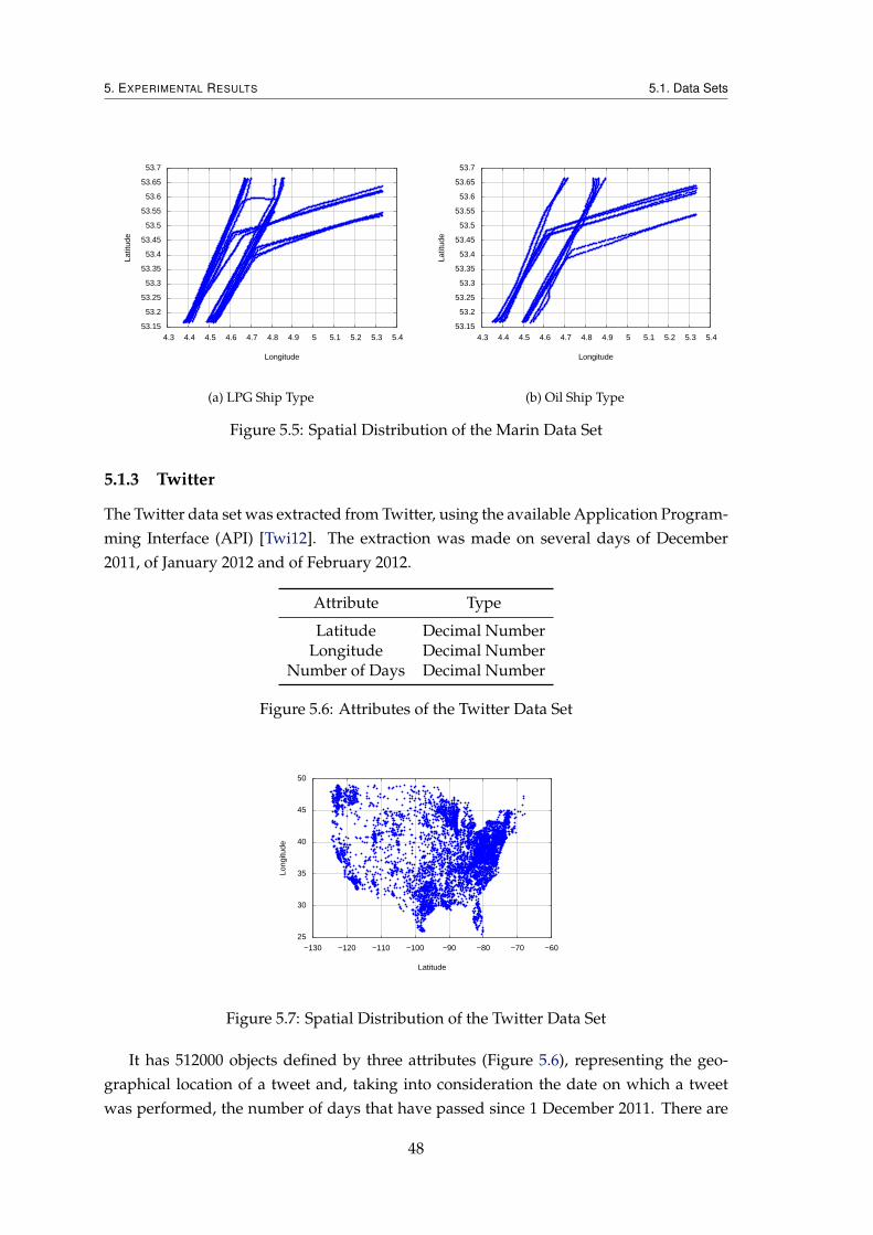
5. EXPERIMENTAL RESULTS 5.1. Data Sets
53.15
53.2
53.25
53.3
53.35
53.4
53.45
53.5
53.55
53.6
53.65
53.7
4.3 4.4 4.5 4.6 4.7 4.8 4.9 5 5.1 5.2 5.3 5.4
Latit
ude
Longitude
(a) LPG Ship Type
53.15
53.2
53.25
53.3
53.35
53.4
53.45
53.5
53.55
53.6
53.65
53.7
4.3 4.4 4.5 4.6 4.7 4.8 4.9 5 5.1 5.2 5.3 5.4
Latit
ude
Longitude
(b) Oil Ship Type
Figure 5.5: Spatial Distribution of the Marin Data Set
5.1.3 Twitter
The Twitter data set was extracted from Twitter, using the available Application Program-ming Interface (API) [Twi12]. The extraction was made on several days of December2011, of January 2012 and of February 2012.
Attribute Type
Latitude Decimal NumberLongitude Decimal Number
Number of Days Decimal Number
Figure 5.6: Attributes of the Twitter Data Set
25
30
35
40
45
50
−130 −120 −110 −100 −90 −80 −70 −60
Long
itude
Latitude
Figure 5.7: Spatial Distribution of the Twitter Data Set
It has 512000 objects defined by three attributes (Figure 5.6), representing the geo-graphical location of a tweet and, taking into consideration the date on which a tweetwas performed, the number of days that have passed since 1 December 2011. There are
48

5. EXPERIMENTAL RESULTS 5.2. kd-SNN
8001 different geographical locations (Figure 5.7). The distance function used was alsothe generic euclidean distance over the three attributes.
This spatio-temporal data set was chosen in order to evaluate the scalability gain ofthe kd-SNN and of the DF-SNN, since it has a meaningful number of objects to be clus-tered.
5.2 kd-SNN
5.2.1 Evaluation of the Quality of the Clustering Results
This evaluation starts with the clustering results obtained when applying the kd-SNNover the synthetic data sets. Two of these results, Synthetic 1 (Figure 5.2a) and Synthetic2 (Figure 5.2b), are compared with the results in [MSC05] obtained with a variant ofthe SNN. The Synthetic 3 (Figure 5.2c) has no benchmarks, since no clustering resultsobtained with the SNN were found in the literature. However, as the clustering tendencycan be visually perceived, the Synthetic 3 was also analysed.
All the presented clustering results have their clusters identified by a unique colorand their noise represented by the black color, except for the Marin data set clusteringresults, where the noise is not shown.
(a) Benchmark [MSC05]
41.13
41.14
41.15
41.16
41.17
41.18
41.19
41.2
41.21
41.22
−8.7 −8.68 −8.66 −8.64 −8.62 −8.6 −8.58 −8.56
Y
X
(b) kd-SNN
Figure 5.8: Clustering Results of the Synthetic 1 Data Set (Evaluation of the kd-SNN)
The clustering results for Synthetic 1 are presented in figure 5.8. On figure 5.8a isshown the benchmark with k = 7, Eps = 0.3 × k, MinPts = 0.7 × k and on figure 5.8b isshown the clustering results obtained with the kd-SNN with k = 7, Eps = 2 and MinPts= 5. As can be seen, both implementations returned the same results for the Synthetic 1data set.
On the other hand, when comparing the benchmark of the Synthetic 2 (Figure 5.9a),having k = 7, Eps = 0.3× k, MinPts = 0.7× k, with the clustering results obtained with thekd-SNN (Figure 5.9b) having k = 7, Eps = 2 and MinPts = 5, there is one slight difference.
49

5. EXPERIMENTAL RESULTS 5.2. kd-SNN
(a) Benchmark [MSC05]
41.19
41.195
41.2
41.205
41.21
41.215
41.22
41.225
−8.675 −8.67 −8.665 −8.66 −8.655 −8.65 −8.645 −8.64 −8.635 −8.63
Y
X
(b) kd-SNN
Figure 5.9: Clustering Results of the Synthetic 2 Data Set (Evaluation of the kd-SNN)
There is one object that was not defined as noise and was clustered, while on its respectivebenchmark it was defined as noise (object inside the dotted circle). It seems that theobject had a density value below the density threshold and it was not identified as noise(remaining object). However, it was clustered, because it had a clustered representativeneighbour with which it shared a higher similarity.
41.196
41.198
41.2
41.202
41.204
41.206
41.208
41.21
41.212
41.214
41.216
−8.675 −8.67 −8.665 −8.66 −8.655 −8.65 −8.645 −8.64 −8.635
Y
X
(a) kd-SNN
Figure 5.10: Clustering Results of the Synthetic 3 Data Set (Evaluation of the kd-SNN)
Differences between some clustering results and their respective benchmarks, maybe due to some minor differences between the implemented variants of the SNN, for in-stance: what to do when there is no representative objects among its neighbours? In thisapproach, the SNN seeks to find a predominant cluster for the object without a repre-sentative neighbour. What if there are two or more most similar representative objectsamong its neighbours and only one can be chosen? In this approach, the first one found
50

5. EXPERIMENTAL RESULTS 5.2. kd-SNN
is the one chosen. It can also be due to different k-nearest neighbours results, for exam-ple, two or more neighbours may share the same distance from the queried object andnot all fit in the final set of k-nearest neighbours, and on each implementation a differentneighbour makes it to the final set of k-nearest neighbours, which in this approach woulddepend on the tiebreaker used by the metric data structure.
When dealing with the Synthetic 3, the clustering results (Figure 5.10a) obtained withk = 7, Eps = 2 and MinPts = 5 are the expected, as they match the clustering tendencyof the data set. These clustering results were not compared with a benchmark, since noresults for this data set were presented in [MSC05] and were not found in the literatureusing the Original SNN or one of its variants.Automated Traffic Route Identification through the SNN Algorithm 13
4.6 4.8 5.0 5.2
53.3
53.4
53.5
53.6
Fig. 8. Clustering results with w=90%, k=12, Eps=3 and MinPts=7
The small clusters that naturally emerged due to the distribution of the
motion vectors can be eliminated in a post-processing stage, as the number of motion vectors that integrate the clusters that represent routes and the other clusters is very different. For example, Fig. 9 presents a histogram with the number of motion vectors per cluster, calling our attention to the huge difference between the number of motion vectors integrated in clus-ters number 1, 2, 3 and 4 when compared with clusters 5, 6, 7, 8, and 9.
Fig. 9. Histogram with the number of motion vectors per cluster
If we look into the interval of the bearing values inside each cluster, we
can see aligned clusters, with a small variation in the bearing values per cluster. Fig. 10 depicts these results. In this figure we can see cluster num-ber 0, representing the motion vectors classified as noise by the SNN algo-rithm, with a huge variation in the bearing value.
(a) Benchmark [SSMPW12]
53.15
53.2
53.25
53.3
53.35
53.4
53.45
53.5
53.55
53.6
53.65
53.7
4.3 4.4 4.5 4.6 4.7 4.8 4.9 5 5.1 5.2 5.3 5.4
Latitude
Longitude
(b) kd-SNN
53.15
53.2
53.25
53.3
53.35
53.4
53.45
53.5
53.55
53.6
53.65
53.7
4.3 4.4 4.5 4.6 4.7 4.8 4.9 5 5.1 5.2 5.3 5.4
Latitude
Longitude
(c) kd-SNN
Figure 5.11: Clustering Results of the LPG Ship Type (Evaluation of the kd-SNN)
Following, the clustering results of the Marin data set are presented, starting with theLPG ship type and, then, the Oil ship type. Despite having the same clustering struc-ture, the clustering results are not exactly the same, for both ship types. Not just someobjects ended up in different clusters, but the user-defined parameters were also slightlyadjusted, trying to obtain more similar results to the respective benchmark. The reasonsbehind these differences may be the ones pointed out before, for the synthetic data sets,since the reasons are tied to the written implementation of the variant of the SNN andnot to the data sets themselves.
51

5. EXPERIMENTAL RESULTS 5.2. kd-SNN
When using the same values for the user-defined parameters of the SNN as in thebenchmark (Figure 5.11a, having k = 12, Eps = 3 and MinPts = 7), the clustering resultshad one main difference. See figure 5.11a for the benchmark results and figure 5.11b forthe kd-SNN results with the same values as the benchmark. Route number 3 and 4 inthe benchmark were just one cluster (yellow cluster) in the kd-SNN results. The clustershould have been split, since the heading of the ships changed. When the MinPts waschanged to 8 (Figure 5.11c), the route was split (yellow and orange clusters), leading tomore similar results. They still have minor differences, for instance, noise points that arenot defined as noise in the benchmark, but the main routes were identified.
Great!
Another type of SHIP: Fishing
Selecting Main Ship Type Chemical (all the available in this dataset), K=12, eps=3, minPoints=7, position=90%, bearing=10%
?? clusters (??? seconds)
4.6 4.8 5.0 5.2
53.3
53.4
53.5
53.6
(a) Benchmark
53.15
53.2
53.25
53.3
53.35
53.4
53.45
53.5
53.55
53.6
53.65
53.7
4.3 4.4 4.5 4.6 4.7 4.8 4.9 5 5.1 5.2 5.3 5.4
Latitude
Longitude
(b) kd-SNN
53.15
53.2
53.25
53.3
53.35
53.4
53.45
53.5
53.55
53.6
53.65
53.7
4.3 4.4 4.5 4.6 4.7 4.8 4.9 5 5.1 5.2 5.3 5.4
Latitude
Longitude
(c) kd-SNN
Figure 5.12: Clustering Results of the Oil Ship Type (Evaluation of the kd-SNN)
With the Oil ship type, the clustering structure of the clustering results obtained withthe kd-SNN was practically equal to the benchmark. See figure 5.12a for the benchmark,taken from the document containing the clustering results provided by the authors, andsee figure 5.12b for the clustering results of the kd-SNN, having k = 12, Eps = 3 and MinPts= 7, the same values as in the benchmark.
There was one difference, as one of the routes was broken (yellow and green clustersin Figure 5.12b), when crossing over another route with a different heading (red cluster).This did not happen in the benchmark with the same user-defined parameters. Whenthe number of k-nearest neighbours was increased by one (Figure 5.12c), trying to get theroute entirely, by accounting one more neighbour (k = 13) that could move the objects
52

5. EXPERIMENTAL RESULTS 5.2. kd-SNN
from the green cluster to the yellow cluster, the cluster was not broken, obtaining thesame routes identified in the benchmark (6 clusters).
5.2.2 Performance Evaluation
To evaluate the scalability of the kd-SNN, the Twitter data set was used, but was brokendown to several subsets of different sizes: 500, 1000, 2000, 4000, 8000, 16000, 32000, 64000,128000, 256000 and 512000, in order to evaluate the performance with these differentsizes.
The SNNAE is not used as a benchmark, because the source code is not publiclyavailable and the experimental results presented in [BJ09] are done with a data set with209 objects. These limitations do not allow a conclusive comparison with the SNNAE.
Since this thesis is focused on evaluating the improvement in the scalability of theSNN and not in finding quality and meaning clusters on the data sets used, and giventhe relevance of the number of neighbours in the SNN, the experimental results weredone with the k = 8 (Eps = 2 and MinPts = 6), k = 10 (Eps = 3 and MinPts = 7)and k = 12 (Eps = 4 and MinPts = 8). The values given to the other user-definedparameters followed the procedure used in [MSC05], where the Eps and the MinPts areequal to 30% and 70% of the k values used, respectively.
0
50
100
150
200
250
0 100000 200000 300000 400000 500000 600000
Tim
e T
aken
(s)
Number of Objects
TNC−NC−−C
Figure 5.13: Runtime of the kd-SNN with k = 12
As it can be seen in figure 5.13, the runtime is decomposed in the three runs pointedout in figure 4.1: Tree, Neighbouring and Clustering (TNC) - the initial run, where it isnecessary to build the metric data structure, query and store the k-nearest neighbours ofeach object, before executing the clustering steps of the SNN; Neighbouring and Clus-tering (-NC) - the run where the metric data structure is already built, but it still needsto query and store the k-nearest neighbours, before the clustering steps of the SNN; andClustering (–C) - the run where the metric data structure is already built and the k-nearestneighbours are already known and only the clustering steps of the SNN are carried out.
In figure 5.13, the runtime taken by the kd-SNN to cluster the several subsets with12-nearest neighbours (k = 12) is represented. It follows that the time spent to build
53

5. EXPERIMENTAL RESULTS 5.2. kd-SNN
the kd-Tree has a significant impact, by comparing the runtime of the TNC run with therequired by the -NC run. This impact is not only related with the time taken to buildthe metric data structure, but it is also due to the time spent in preprocessing the Twitterdata set before each object is indexed in the kd-Tree. Regarding the -NC run and the –Crun, its noticeable the effective impact that acquiring the k-nearest neighbours has on theruntime of the kd-SNN.
Regarding the impact of the number of neighbours, see figure 5.14a for the runtimevalues and figure 5.14b for the ratio Runtime of the -NC Run
Runtime of the TNC Run and the ratio Runtime of the –C RunRuntime of the TNC Run ,
for each of the number of neighbours. Taking into consideration that the TNC run andthe -NC run have a time complexity in the average case ofO(n×log n) and that the –C runhas a time complexity in the worst case ofO(n), then the proportions of the -NC ratio andthe –C ratio should not be the same and should not be constant as the number of objectsgrows, which is verified in these experimental results. The -NC ratio was considerablythe same along the different number of objects, as it ranged around 60%. As for the –Cratio, its values are less significant and it supports the O(n × log n) time complexity inthe average case of the TNC run, since as the number of objects is increased, the –C ratiovalues start to tend towards the same values.
0
50
100
150
200
250
0 100000 200000 300000 400000 500000 600000
Tim
e T
aken
(s)
Number of Objects
k = 8 (TNC)k = 8 (−NC)k = 8 (−−C)
k = 10 (TNC)k = 10 (−NC)k = 10 (−−C)k = 12 (TNC)k = 12 (−NC)k = 12 (−−C)
(a) Runtime
0
0.2
0.4
0.6
0.8
1
0 100000 200000 300000 400000 500000 600000
Rat
io
Number of Objects
k = 8k = 10k = 12
-NC
--C
(b) Ratio
Figure 5.14: Runtime of the kd-SNN with k = 8, k = 10 and k = 12
Now, the TNC run of the kd-SNN is compared with the runtime of the referencedimplementation of the Original SNN [ESK03]. In the benchmarking tests the implemen-tation of the Original SNN was run with k = 12, but with the rest of the parametersinvolved in its implementation as default. In figure 5.15a, the runtime of the OriginalSNN and of the kd-SNN are presented, showing the quadratic behaviour of the OriginalSNN. Since the Original SNN takes a significant runtime, it was not evaluated for a dataset above 128000 objects. However, this did not compromise the benchmarking test, as itis still perceived the improvement obtained with the kd-SNN.
On figure 5.15b, the ratio, Runtime of the Original SNNRuntime of the TNC Run of the kd-SNN , reveals that for a spatial data
set with 128000 objects, the runtime of the Original SNN was around 300 times higher
54

5. EXPERIMENTAL RESULTS 5.3. DF-SNN
0
1000
2000
3000
4000
5000
6000
7000
8000
9000
0 100000 200000 300000 400000 500000 600000
Tim
e T
aken
(s)
Number of Objects
Original SNNkd−SNN (TNC)
(a) Runtime
0
50
100
150
200
250
300
350
0 20000 40000 60000 80000 100000 120000 140000
Rat
io
Number of Objects
Ratio
(b) Ratio
Figure 5.15: Runtime of the Original SNN and of the TNC run of the kd-SNN with k = 12
than the runtime of the kd-SNN, granting a distinct improvement in the scalability of theSNN algorithm, when using the kd-SNN to cluster this data set.
5.3 DF-SNN
5.3.1 Evaluation of the Quality of the Clustering Results
Bearing in mind the procedure of evaluation taken with the kd-SNN, the same procedureis carried out in the evaluation of the DF-SNN. First, the clustering results of the syntheticdata sets are evaluated and, then, the two Marin data sets that represent the LPG and Oilship types.
(a) Benchmark [MSC05]
41.13
41.14
41.15
41.16
41.17
41.18
41.19
41.2
41.21
41.22
−8.7 −8.68 −8.66 −8.64 −8.62 −8.6 −8.58 −8.56
Y
X
(b) DF-SNN
Figure 5.16: Clustering Results of the Synthetic 1 Data Set (Evaluation of the DF-SNN)
The Synthetic 1 still got the same clustering results as with the kd-SNN (Figure 5.8b).On figure 5.16a the benchmark is shown with k = 7, Eps = 0.3 × k, MinPts = 0.7 × k and
55
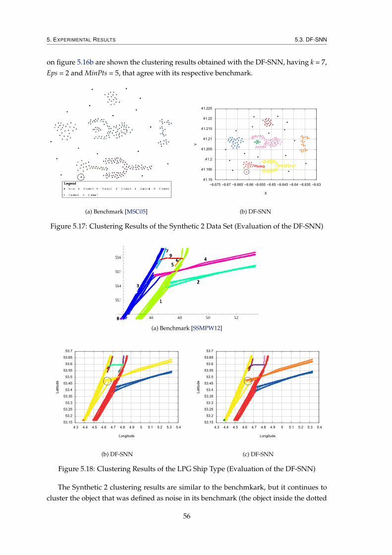
5. EXPERIMENTAL RESULTS 5.3. DF-SNN
on figure 5.16b are shown the clustering results obtained with the DF-SNN, having k = 7,Eps = 2 and MinPts = 5, that agree with its respective benchmark.
(a) Benchmark [MSC05]
41.19
41.195
41.2
41.205
41.21
41.215
41.22
41.225
−8.675 −8.67 −8.665 −8.66 −8.655 −8.65 −8.645 −8.64 −8.635 −8.63
YX
(b) DF-SNN
Figure 5.17: Clustering Results of the Synthetic 2 Data Set (Evaluation of the DF-SNN)Automated Traffic Route Identification through the SNN Algorithm 13
4.6 4.8 5.0 5.2
53.3
53.4
53.5
53.6
Fig. 8. Clustering results with w=90%, k=12, Eps=3 and MinPts=7
The small clusters that naturally emerged due to the distribution of the
motion vectors can be eliminated in a post-processing stage, as the number of motion vectors that integrate the clusters that represent routes and the other clusters is very different. For example, Fig. 9 presents a histogram with the number of motion vectors per cluster, calling our attention to the huge difference between the number of motion vectors integrated in clus-ters number 1, 2, 3 and 4 when compared with clusters 5, 6, 7, 8, and 9.
Fig. 9. Histogram with the number of motion vectors per cluster
If we look into the interval of the bearing values inside each cluster, we
can see aligned clusters, with a small variation in the bearing values per cluster. Fig. 10 depicts these results. In this figure we can see cluster num-ber 0, representing the motion vectors classified as noise by the SNN algo-rithm, with a huge variation in the bearing value.
(a) Benchmark [SSMPW12]
53.15
53.2
53.25
53.3
53.35
53.4
53.45
53.5
53.55
53.6
53.65
53.7
4.3 4.4 4.5 4.6 4.7 4.8 4.9 5 5.1 5.2 5.3 5.4
Latitude
Longitude
(b) DF-SNN
53.15
53.2
53.25
53.3
53.35
53.4
53.45
53.5
53.55
53.6
53.65
53.7
4.3 4.4 4.5 4.6 4.7 4.8 4.9 5 5.1 5.2 5.3 5.4
Latitude
Longitude
(c) DF-SNN
Figure 5.18: Clustering Results of the LPG Ship Type (Evaluation of the DF-SNN)
The Synthetic 2 clustering results are similar to the benchmkark, but it continues tocluster the object that was defined as noise in its benchmark (the object inside the dotted
56
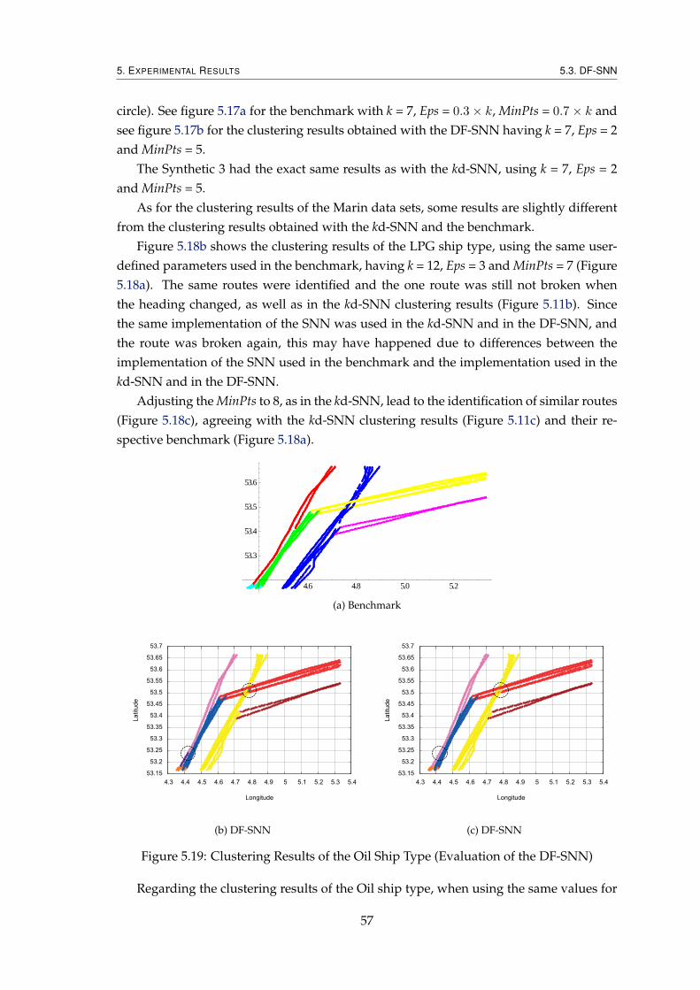
5. EXPERIMENTAL RESULTS 5.3. DF-SNN
circle). See figure 5.17a for the benchmark with k = 7, Eps = 0.3× k, MinPts = 0.7× k andsee figure 5.17b for the clustering results obtained with the DF-SNN having k = 7, Eps = 2and MinPts = 5.
The Synthetic 3 had the exact same results as with the kd-SNN, using k = 7, Eps = 2and MinPts = 5.
As for the clustering results of the Marin data sets, some results are slightly differentfrom the clustering results obtained with the kd-SNN and the benchmark.
Figure 5.18b shows the clustering results of the LPG ship type, using the same user-defined parameters used in the benchmark, having k = 12, Eps = 3 and MinPts = 7 (Figure5.18a). The same routes were identified and the one route was still not broken whenthe heading changed, as well as in the kd-SNN clustering results (Figure 5.11b). Sincethe same implementation of the SNN was used in the kd-SNN and in the DF-SNN, andthe route was broken again, this may have happened due to differences between theimplementation of the SNN used in the benchmark and the implementation used in thekd-SNN and in the DF-SNN.
Adjusting the MinPts to 8, as in the kd-SNN, lead to the identification of similar routes(Figure 5.18c), agreeing with the kd-SNN clustering results (Figure 5.11c) and their re-spective benchmark (Figure 5.18a).
Great!
Another type of SHIP: Fishing
Selecting Main Ship Type Chemical (all the available in this dataset), K=12, eps=3, minPoints=7, position=90%, bearing=10%
?? clusters (??? seconds)
4.6 4.8 5.0 5.2
53.3
53.4
53.5
53.6
(a) Benchmark
53.15
53.2
53.25
53.3
53.35
53.4
53.45
53.5
53.55
53.6
53.65
53.7
4.3 4.4 4.5 4.6 4.7 4.8 4.9 5 5.1 5.2 5.3 5.4
Latitude
Longitude
(b) DF-SNN
53.15
53.2
53.25
53.3
53.35
53.4
53.45
53.5
53.55
53.6
53.65
53.7
4.3 4.4 4.5 4.6 4.7 4.8 4.9 5 5.1 5.2 5.3 5.4
Latitude
Longitude
(c) DF-SNN
Figure 5.19: Clustering Results of the Oil Ship Type (Evaluation of the DF-SNN)
Regarding the clustering results of the Oil ship type, when using the same values for
57

5. EXPERIMENTAL RESULTS 5.3. DF-SNN
the user-defined parameters used in its benchmark with k = 12, Eps = 3 and MinPts = 7(Figure 5.19a), in the clustering results (Figure 5.19b) the route was still broken in two(yellow and green clusters) when it crossed the route with a different heading (red clus-ter), as in the clustering results of the kd-SNN (Figure 5.12b). In addition, these clusteringresults also broke another route in two (violet and pink clusters), which did not happenin the kd-SNN clustering results. Since the same SNN implementation was used, this isdue to differences in the k-nearest neighbours given by each of the metric data structures.
When the number of neighbours was increased by one (k = 13), the clustering results(Figure 5.19c) were similar to the kd-SNN clustering results (Figure 5.12c) and similar tothe routes identified in the benchmark.
5.3.2 Performance Evaluation
The evaluation procedure carried out with the kd-SNN was the same that was taken withthe DF-SNN. However, since the runtime of the TNC run of the DF-SNN is greater thanits remaining runs, as it will be seen, the TNC run will be plotted in a different chart, inorder not to compromise the interpretation and evaluation of the runtime of the -NC runand of the –C run.
The runtime of the DF-SNN is decomposed in the three runs pointed out in figure4.1, however in the DF-SNN, besides the runtime of building the metric data structure,querying it and doing the clustering, it also accounts the runtime of deploying the SQLfile, importing it to the DBMS and obtaining the k-nearest neighbours from the DBMS.
The Tree, Neighbouring and Clustering (TNC) run is the initial run, where it is nec-essary to build the metric data structure, query it for the k-nearest neighbours, deployand import the SQL file to the DBMS. These operations are all part of the secondarystorage component. Then, the primary storage component accesses the DBMS to get thek-nearest neighbours and does the clustering. The Neighbouring and Clustering (-NC)run accounts the time of getting the k-nearest neighbours, deploying and importing theSQL file to the DBMS, getting the k-nearest neighbours and, for last, clustering the dataset. At last, the Clustering (–C) represents just the runtime of clustering the data set, sinceit does not require an access to the DBMS, since the k-nearest neighbours are already inprimary storage.
In figure 5.20a it is shown the runtime of the TNC run of the DF-SNN, with 12-nearestneighbours. By comparing the runtime taken by the TNC run and the remaining two runs(Figure 5.20b), it is perceived that the runtime of getting the k-nearest neighbours fromthe DF-Tree, deploying and importing the SQL file, getting the k-nearest neighbours fromthe DBMS and clustering the data set, represented a very small part of the total runtimeof the TNC run of the DF-SNN, leading the secondary storage component to the primarysource of the runtime of the DF-SNN. Regarding the runtime required for the importingof the SQL file with the objects and their respective k-nearest neighbours (Figure 5.21) tothe DBMS with 128000 objects, the importing took 0.7% of the runtime of the TNC run,
58

5. EXPERIMENTAL RESULTS 5.3. DF-SNN
0
1000
2000
3000
4000
5000
6000
7000
8000
9000
0 20000 40000 60000 80000 100000 120000 140000
Tim
e T
aken
(s)
Number of Objects
TNC
(a) DF-SNN (TNC)
0
20
40
60
80
100
120
140
0 20000 40000 60000 80000 100000 120000 140000
Tim
e T
aken
(s)
Number of Objects
−NC−−C
(b) DF-SNN (-NC and –C)
Figure 5.20: Runtime of the DF-SNN with k = 12
representing a very small part of the runtime. The weight of importing became smalleras the data set size was increased, since the weight of building the tree became biggerwith the number of objects in the data set.
As for the -NC run, it started to have an increase in its runtime as the size of thedata set increased, not only because of the growing runtime required to get the k-nearestneighbours, but also due to the increasing number of rows that needed to be inserted inthe DBMS. For example, with 128000 objects, it needed to input 1536000 rows with the k-nearest neighbours of each object, plus the 128000 rows with the objects attributes. Sincethe -NC run took less time than the TNC run, the weight of importing the SQL file to theDBMS had a bigger role in the runtime of the -NC run (Figure 5.21), for instance, with128000 objects, the weight was approximately 50% and for the remaining data set sizes,the weight was always around the same range of values.
Data Set Runtime of Importing on theSize TNC Run -NC Run
500 26.5% 37.1%1000 18.4% 30.6%2000 19.1% 46.7%4000 18.0% 54.1%8000 7.9% 51.6%16000 2.5% 50.4%32000 0.8% 53.9%64000 0.3% 46.9%128000 0.7% 46.3%
Figure 5.21: Weight of Importing the SQL file to the DBMS
It is concluded that, the runtime of the DF-SNN was not as promising as the runtimeobtained with the kd-SNN, namely the TNC run. This was somehow expected, due to the
59

5. EXPERIMENTAL RESULTS 5.3. DF-SNN
distinct nature of each of the metric data structures, as the kd-Tree works in primary stor-age and the DF-Tree works in secondary storage, where the last demands higher accesstimes.
As it is presented in figure 5.22, the number of accesses made by the DF-Tree to thesecondary storage, became more and more significant as the data set size increased. Thisis due to the outgrowth of the tree size, leading to a much more deeper and larger tree.Not only this had an impact in the tree building, but it also complicated the whole an-swering process of the k-nearest neighbours queries, since more sub-trees needed to beexplored and they were in different pages 1 that constantly need to be acquired from thesecondary storage. This lead to an increase of the runtime, namely of the TNC run, whenthe data set had a magnitude higher than 16000 objects, becoming proportional to thenumber of secondary storage accesses.
Data Set No. of Secondary Storage AccessesSize Building Querying
500 13633 58281000 45112 155542000 169668 407914000 674122 1281398000 2644085 32097316000 10305032 91015832000 40709616 266498064000 160820199 7323828
Figure 5.22: No. of Secondary Storage Accesses by the DF-Tree with k = 12
As the number of neighbours changed between the range of 8-nearest neighbours(k = 8), 10-nearest neighbours (k = 10) and 12-nearest neighbours (k = 12), the runtimeof the DF-SNN was essentially the same (Figure 5.23), despite of the number of k-nearestneighbours used.
It seems that the runtime of the TNC run was not that affected with the change in thenumber of neighbours, at least with the values used (Figure 5.23a). On the other hand,despite not representing a significant difference in the runtime, since it is smaller than theruntime of the TNC run, the -NC run and the –C run were more sensitive to the varianceof the number of neighbours. The -NC run was sensitive to the number of neighbours,because more rows needed to be inserted in the DBMS and then retrieved from the DBMSby the primary storage component. For instance, with 64000 objects and k = 12, therewere 768000 rows that needed to be read, but with the same number of objects and k = 8,there were only 512000 rows, which is 2
3 of the number of rows with k = 12. The –C runwas also sensitive, since the number of neighbours has impact on the SNN algorithm.
On figure 5.23c, the ratio Runtime of the -NC RunRuntime of the TNC Run and the ratio Runtime of the –C Run
Runtime of the TNC Run are
1Buffers of secondary storage-backed pages temporarily kept in primary storage by the operating systemfor quicker access and analysis.
60

5. EXPERIMENTAL RESULTS 5.3. DF-SNN
0
1000
2000
3000
4000
5000
6000
7000
8000
9000
0 20000 40000 60000 80000 100000 120000 140000
Tim
e T
aken
(s)
Number of Objects
k = 8 (TNC)k = 10 (TNC)k = 12 (TNC)
(a) DF-SNN (TNC)
0
20
40
60
80
100
120
140
0 20000 40000 60000 80000 100000 120000 140000
Tim
e T
aken
(s)
Number of Objects
k = 8 (−NC)k = 8 (−−C)
k = 10 (−NC)k = 10 (−−C)k = 12 (−NC)k = 12 (−−C)
(b) DF-SNN (-NC and –C)
0
0.1
0.2
0.3
0.4
0.5
0.6
0.7
0.8
0 20000 40000 60000 80000 100000 120000 140000
Rat
io
Number of Objects
k = 8 (−NC) Ratiok = 8 (−−C) Ratio
k = 10 (−NC) Ratiok = 10 (−−C) Ratiok = 12 (−NC) Ratiok = 12 (−−C) Ratio
(c) Ratio
Figure 5.23: Runtime of the DF-SNN with k = 8, k = 10 and k = 12
shown, for the several k values. As already pointed out, it is concluded, by looking atthe figure, that the runtime of the primary storage component was not significant in thetotal runtime of the DF-SNN, leading the total runtime of the DF-SNN to be dependent ofthe runtime of the secondary storage component, even with the variance in the numberof neighbours.
In figure 5.24, the runtime of the DF-SNN is compared with the runtime of the Orig-inal SNN, showing a not so good improvement in the scalability of the Original SNN(Figure 5.24a).
Initially, with a data set with less than 4000 objects, the DF-SNN was not able toachieve an improvement over the Original SNN, as the ratio, Runtime of the Original SNN
Runtime of the DF-SNN , wasbelow 100%. With a data set with a magnitude between 4000 and 8000 objects, the DF-SNN had an improvement of approximately 5% over the Original SNN. However, whenthe number of objects was above 8000 objects, there was a breaking point of this pattern,where the improvement started to decrease to none and the DF-SNN became, again,worse than the Original SNN. When it reached 128000 objects, the DF-SNN recovered
61
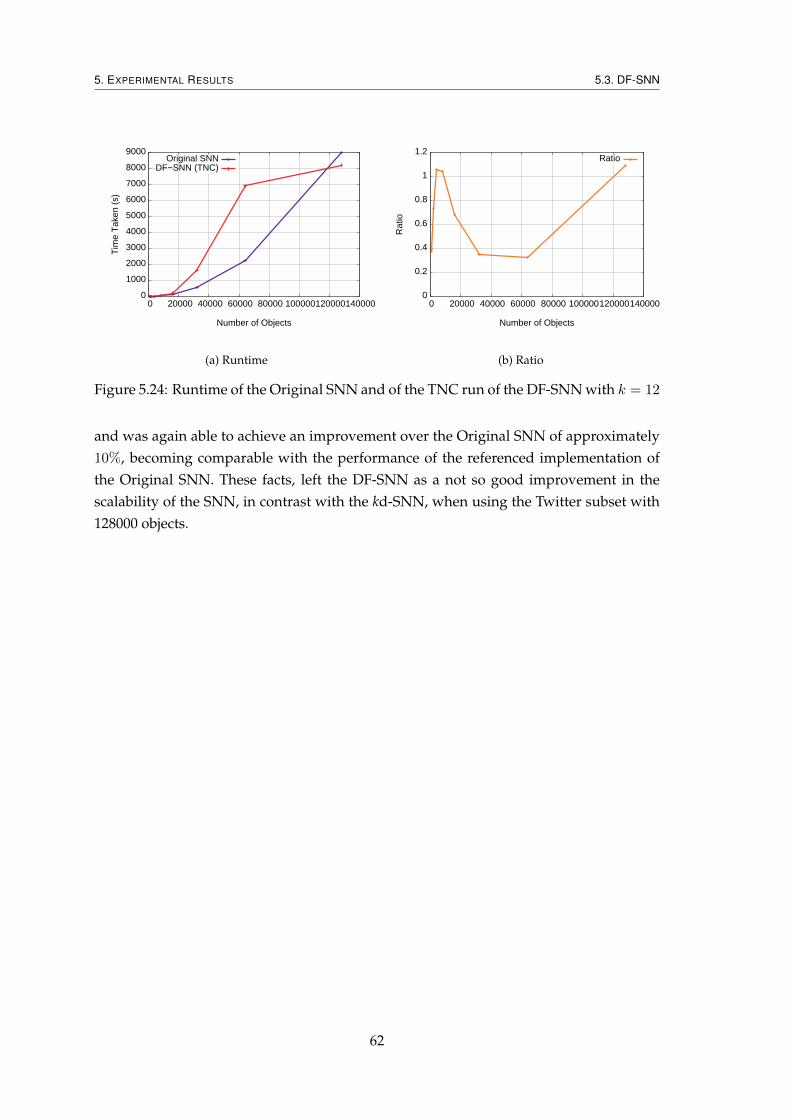
5. EXPERIMENTAL RESULTS 5.3. DF-SNN
0
1000
2000
3000
4000
5000
6000
7000
8000
9000
0 20000 40000 60000 80000 100000 120000 140000
Tim
e T
aken
(s)
Number of Objects
Original SNNDF−SNN (TNC)
(a) Runtime
0
0.2
0.4
0.6
0.8
1
1.2
0 20000 40000 60000 80000 100000 120000 140000
Rat
io
Number of Objects
Ratio
(b) Ratio
Figure 5.24: Runtime of the Original SNN and of the TNC run of the DF-SNN with k = 12
and was again able to achieve an improvement over the Original SNN of approximately10%, becoming comparable with the performance of the referenced implementation ofthe Original SNN. These facts, left the DF-SNN as a not so good improvement in thescalability of the SNN, in contrast with the kd-SNN, when using the Twitter subset with128000 objects.
62

6Conclusions
This thesis proposes an implementation of the SNN clustering algorithm to deal withspatial data. It uses metric data structures to support the k-nearest neighbours queries ofthe SNN and, consequently, improve the scalability of the algorithm, since it currently hasa O(n2) time complexity in the worst case. Bear in mind that this approach is applicableto all clustering algorithms that require the k-nearest neighbours of each object for itsclustering process.
The scalability of clustering algorithms is important, because these type of algorithmsrequire multiple runs to do the fine-tuning of the user-defined parameters, in order toachieve the best possible clustering results.
Two distinct implementations were made, taking advantage of different metric datastructures: one implementation using the kd-Tree, which works in primary storage, andanother implementation using the DF-Tree, which, on the other hand, works in secondarystorage. Each of these metric data structures index the data sets and reply with the resultsof the k-nearest neighbours queries of each object in the indexed data set.
For low dimensional data, namely when dealing with spatial data, the proposed pri-mary storage implementation improved the time complexity in the average case of theSNN to at most O(n× log n): on an initial run, where it is necessary to build the kd-Tree,query it for the k-nearest neighbours and run the SNN; or on a run following the initial,where the kd-Tree is already built and it needs to be queried again for more k-nearestneighbours and run the SNN. When there is no need to query for more k-nearest neigh-bours and the SNN is the only step executed, reusing the previously calculated k-nearestneighbours, the time complexity in the worst case can be improved to O(n).
The experimental results of the primary storage approach evaluated the quality andvalidity of the clustering results and the improvement in its scalability. In order to make
63

6. CONCLUSIONS
the evaluation of the clustering results, three synthetic and two real data sets and their re-spective clustering results obtained with another implementation of the SNN, were used.To measure the improvement in the scalability of the SNN, the runtime of the primarystorage implementation was compared with the runtime of a referenced implementationin the literature of the SNN.
The primary storage implementation returned similar clustering results for the datasets used, when compared to their respective benchmarks.
The performance results of the primary storage implementation showed a good im-provement in the scalability of the SNN, when compared with the referenced implemen-tation. The initial run improved the scalability of the SNN, substantiating the improve-ment in its scalability, as it clustered a three-dimensional data set with 128000 objectsusing 12-nearest neighbours, 300 times faster than the referenced implementation. How-ever, in the following runs, using a strategy over the user-defined parameters, startingwith a higher number of k-nearest neighbours, the primary storage implementation waseven more faster. If the algorithm starts with a higher number of k-nearest neighbours,and then, in the following runs, the number is adjusted downward, the runtime to querythe metric data structure for more k-nearest neighbours can be avoided, only executingthe SNN algorithm, which is significantly faster than the initial run, as it only takes 10%
of the runtime of the initial run. However, the improvement in these performance re-sults may start to decrease as the dimensionality of a data set grows, since the theoreticalresults of the time complexity of the kd-Tree involve the dimensionality of a data set,which when not in a low dimensionality scenario, may start to affect the scalability of thekd-Tree, compromising its performance and, consequently, the performance of the SNN.
Regarding these primary storage implementation results, a paper [FMPS12] with theseresults was submitted and accepted on the INForum 2012, a Portuguese annual sympo-sium on computer science, applied informatics and information technology.
On the other hand, the secondary storage implementation did not obtain such promis-ing results as the primary storage implementation. It still got similar clustering resultsfor the used data sets, when compared to their respective benchmarks. However, onlywith a three-dimensional data set with 128000 objects using 12-nearest neighbours, thesecondary storage approach was able to obtain a runtime of the initial run comparablewith the referenced implementation, improving the runtime in approximately 10%. Withfewer objects, only with 4000 and 8000 objects, the secondary storage approach got abetter runtime, with an improvement of approximately 5%. The referred strategy overthe user-defined parameters also applies to this secondary storage implementation. Inthe experimental results, the following runs obtained a greater time than the initial run.With 128000 objects and using 12-nearest neighbours, the following runs took less than0.05% of the time of the initial run, where only the SNN algorithm is executed. It followsthat, this approach should also start with a higher number of neighbours, and then, theSNN can have a bigger leeway regarding the number of neighbours that can be used andthat are stored in the database.
64

6. CONCLUSIONS
Despite the fact that the DF-Tree does not have their time complexity evaluated, someexperimental results taken showed that the kd-Tree requires a lot more distance calcu-lations than the DF-Tree. This leads to believe that the DF-Tree may handle more thegrowth of the dimensionality of a data set, when compared with the kd-Tree. These as-sertions could be validated by making several evaluations with data sets with a differentdimensionality.
So, to reinforce the results of this thesis, several evaluations could be done:
• evaluate the influence of the dimensionality of the data sets over the runtime. In thisexperimental results, the runtime was evaluated with a three-dimensional data setwith numeric attributes. However, some experimental results could be obtained,using data sets with more attributes, numerical or alphanumerical, to obtain a bet-ter perception of how the growth of the dimensionality reduces the gains of theimplementations of the SNN using the primary and secondary storage approaches;
• evaluate the effect of the domain size of the data set attributes on the runtime. Ex-perimental results could be obtained, using data sets that have attributes with alarger domain size, in order to perceive the impact that it has over the runtimeof the implementations of the SNN using the primary and secondary storage ap-proaches;
• evaluate the impact of using different data sets over the runtime. Every data set hasa clustering tendency and, consequently, an impact over the runtime of the SNN,since every data set has a specific set of values for the user-defined parameters ofthe SNN, that lead to specific clustering results. The goal would be to evaluatehow a specific data set with a specific set of values for the user-defined parametersof the SNN has impact on the runtime of the implementations of the SNN usingthe primary and secondary storage approaches, while evaluating the influence ofthe variation of the values of the Eps and the MinPts, the remaining user-definedparameters of the SNN.
Besides the above evaluations, since the scope of this thesis was later focused on spa-tial data, some experimental results with spatial data metric data structures could havebe done, in order to evaluate the performance obtained with these type of metric datastructures, for instance, the R-Tree [Gut84]. The future work can involve evaluating theperformance with these type of metric data structures and, due to the results obtainedwith the runtime of the primary storage implementation, some future work can also bedone towards the tuning of the user-defined parameters:
• auto-tuning - if there are enough resources to establish an evaluation criteria of theclustering results, the SNN can be adjusted to make an auto-tuning of the user-defined parameters, as it produces the clustering results, in order to find the bestpossible clustering results in a timely manner;
65

6. CONCLUSIONS
• interactive-tuning - this solution fits in the research area of Geovisual Analytics[AAJ+07], which seeks to find ways to engage the user to provide computer sup-port to solve spatial-related decision problems, by enhancing human capabilities toreason and analyse the output that is given by the computer. The runtime obtained,strengthens the idea of an interactive solution, where the interaction between theuser input of the values of the user-defined parameters of the SNN and the cluster-ing results, can be done in a timely manner, going towards the idea of GeovisualAnalytics.
66

Bibliography
[Ža11] Borut Žalik. Validity index for clusters of different sizes and densities. Pat-tern Recognition Letters, 32(2):221–234, 2011.
[AAJ+07] G. Andrienko, N. Andrienko, P. Jankowski, D. Keim, M. J. Kraak,A. MacEachren, and S. Wrobel. Geovisual analytics for spatial decisionsupport: Setting the research agenda. Int. J. Geogr. Inf. Sci., 21(8):839–857,January 2007.
[BCKO10] Mark de Berg, Otfried Cheong, Marc van Kreveld, and Mark Overmars.Computational Geometry: Algorithms and Applications. Springer, softcoverreprint of hardcover 3rd ed. 2008 edition, November 2010.
[Ben75] Jon Louis Bentley. Multidimensional binary search trees used for associativesearching. Commun. ACM, 18(9):509–517, September 1975.
[BJ09] H. B Bhavsar and A. G Jivani. The shared nearest neighbor algorithm withenclosures (SNNAE). In 2009 WRI World Congress on Computer Science andInformation Engineering, volume 4, pages 436–442. IEEE, April 2009.
[Bur10] Stephen D. Burd. Systems Architecture. Cengage Learning, August 2010.
[CNBYM01] Edgar Chávez, Gonzalo Navarro, Ricardo Baeza-Yates, and José Luis Mar-roquín. Searching in metric spaces. ACM Comput. Surv., 33(3):273–321,September 2001.
[CPZ97] Paolo Ciaccia, Marco Patella, and Pavel Zezula. M-tree: An efficient accessmethod for similarity search in metric spaces. Processing, Athens, Gr:426–435, 1997.
[Dat06] Databases and Images Group. Downloads | databases and images group.http://www.gbdi.icmc.usp.br/en/download, August 2006.
67

BIBLIOGRAPHY
[dCFLH04] Luis M de Campos, Juan M Fernández-Luna, and Juan F Huete. Bayesiannetworks and information retrieval: an introduction to the special issue.Information Processing & Management, 40(5):727–733, September 2004.
[DHS00] Richard O. Duda, Peter E. Hart, and David G. Stork. Pattern Classification.Wiley-Interscience, 2 edition, October 2000.
[EKSX96] Martin Ester, Hans-peter Kriegel, Jörg Sander, and Xiaowei Xu. A density-based algorithm for discovering clusters in large spatial databases withnoise. Computer, 1996(6):226–231, 1996.
[ESK03] Levent Ertöz, Michael Steinbach, and Vipin Kumar. Finding clusters of dif-ferent sizes, shapes, and densities in noisy, high dimensional data. In Pro-ceedings of Second SIAM International Conference on Data Mining, 2003.
[FBF77] Jerome H. Friedman, Jon Louis Bentley, and Raphael Ari Finkel. An algo-rithm for finding best matches in logarithmic expected time. ACM Trans.Math. Softw., 3(3):209–226, September 1977.
[Fer07] Olivier Ferret. Finding document topics for improving topic segmentation.2007.
[FMPS12] Bruno Filipe Faustino, João Moura-Pires, and Maribel Yasmina Santos. Im-plementação eficiente do shared nearest neighbour em dados espaciais. InAntónia Lopes and José Orlando Pereira, editors, Proceedings of INForum2012, pages 476–479, Monte da Caparica, Portugal, September 2012. Uni-versidade Nova de Lisboa.
[FSTR06] A. M Fahim, A. M Salem, F. A Torkey, and M. A Ramadan. Density clus-tering algorithm based on radius of data (DCBRD). Computer Sciences andTelecommunications, (4):32–43, 2006.
[GMW07] Guojun Gan, Chaoqun Ma, and Jianhong Wu. Data Clustering: Theory, Al-gorithms, and Applications. SIAM, Society for Industrial and Applied Math-ematics, May 2007.
[Goo12] Google Developers. Protocol buffers. https://developers.google.
com/protocol-buffers/, April 2012.
[GRS98] Sudipto Guha, Rajeev Rastogi, and Kyuseok Shim. CURE: an efficientclustering algorithm for large databases. In Proceedings of the 1998 ACMSIGMOD international conference on Management of data, SIGMOD ’98, page73–84, New York, NY, USA, 1998. ACM.
[Gut84] Antonin Guttman. R-trees: a dynamic index structure for spatial searching.SIGMOD Rec., 14(2):47–57, June 1984.
68

BIBLIOGRAPHY
[GXZ+11] Yong Ge, Hui Xiong, Wenjun Zhou, Siming Li, and Ramendra Sahoo. Mul-tifocal learning for customer problem analysis. ACM Trans. Intell. Syst. Tech-nol., 2(3):24:1–24:22, May 2011.
[HBV02a] Maria Halkidi, Yannis Batistakis, and Michalis Vazirgiannis. Cluster valid-ity methods: part i. SIGMOD Rec., 31(2):40–45, June 2002.
[HBV02b] Maria Halkidi, Yannis Batistakis, and Michalis Vazirgiannis. Clustering va-lidity checking methods: part II. SIGMOD Rec., 31(3):19–27, September2002.
[HFH+09] Mark Hall, Eibe Frank, Geoffrey Holmes, Bernhard Pfahringer, Peter Reute-mann, and Ian H. Witten. The WEKA data mining software: An update.SIGKDD Explorations, 11(1), 2009.
[JP73] R. A Jarvis and E. A Patrick. Clustering using a similarity measure basedon shared near neighbors. IEEE Transactions on Computers, C-22(11):1025–1034, November 1973.
[KHK99] G. Karypis, Eui-Hong Han, and V. Kumar. Chameleon: hierarchical cluster-ing using dynamic modeling. Computer, 32(8):68–75, August 1999.
[KI06] Ferenc Kovács and Renáta Iváncsy. Cluster validity measurement for ar-bitrary shaped clusters. In Proceedings of the 5th WSEAS International Con-ference on Artificial Intelligence, Knowledge Engineering and Data Bases, page372–377, Stevens Point, Wisconsin, USA, 2006. World Scientific and Engi-neering Academy and Society (WSEAS).
[Lia99] Sheng Liang. JavaTM Native Interface: Programmer’s Guide and Specification.Prentice Hall, 1 edition, June 1999.
[Lov04] Alen Lovrencic. maximally connected component. http://xlinux.
nist.gov/dads/HTML/maximallyConnectedComponent.html, De-cember 2004.
[Mac67] JB Macqueen. Some methods of classification and analysis of multivariateobservations. In Proceedings of the Fifth Berkeley Symposium on MathematicalStatistics and Probability, pages 281–297, 1967.
[Mar06] David Marshall. Nearest neighbour searching in high dimensional metricspace. Technical report, 2006.
[MG09] Jeremy Mennis and Diansheng Guo. Spatial data mining and geographicknowledge discovery—An introduction. Computers Environment and UrbanSystems, 33(6):403–408, 2009.
69
BIBLIOGRAPHY
[MH09] Harvey J. Miller and Jiawei Han. Geographic Data Mining and KnowledgeDiscovery, Second Edition. CRC Press, 2 edition, May 2009.
[MSC05] Adriano Moreira, Maribel Yasmina Santos, and Sofia Carneiro. Density-based clustering algorithms – DBSCAN and SNN. http://get.dsi.
uminho.pt/local/download/SNN&DBSCAN.pdf, July 2005.
[MTJ06] Wannes Meert, Remko Tronçon, and Gerda Janssens. Clustering maps.2006.
[NUP11] Gonzalo Navarro and Roberto Uribe-Paredes. Fully dynamic metric accessmethods based on hyperplane partitioning. Inf. Syst., 36(4):734–747, June2011.
[Pat99] Marco Patella. Similarity Search in Multimedia Databases. PhD thesis, Dipar-timento di Elettronica Informatica e Sistemistica, Università degli Studi diBologna, Bologna, Italy, February 1999.
[PB07] Oscar Pedreira and Nieves R. Brisaboa. Spatial selection of sparse pivotsfor similarity search in metric spaces. In Proceedings of the 33rd conference onCurrent Trends in Theory and Practice of Computer Science, SOFSEM ’07, page434–445, Berlin, Heidelberg, 2007. Springer-Verlag.
[RPN+08] Salvatore Rinzivillo, Dino Pedreschi, Mirco Nanni, Fosca Giannotti, NataliaAndrienko, and Gennady Andrienko. Visually driven analysis of move-ment data by progressive clustering. Information Visualization, 7(3):225–239,June 2008.
[Sar10] Ângelo Miguel Loureiro Sarmento. Estruturas de dados métricas genéricas emmemória secundária. MSc thesis, Departamento de Informática, Universi-dade Nova de Lisboa, 2010.
[Sav12] Savarese Software Research Corporation. libssrckdtree-j generic k-d tree java library. http://www.savarese.com/software/
libssrckdtree-j/, 2012.
[SB11] Tomáš Skopal and Benjamin Bustos. On nonmetric similarity search prob-lems in complex domains. ACM Comput. Surv., 43(4):34:1–34:50, October2011.
[SKN07] Kalyankumar Shencottah K. N. Finding Clusters in Spatial Data. MSc thesis,University of Cincinnati, 2007.
[SMO11] Raisa Socorro, Luisa Micó, and Jose Oncina. A fast pivot-based indexingalgorithm for metric spaces. Pattern Recognition Letters, 32(11):1511–1516,August 2011.
70
BIBLIOGRAPHY
[SSMPW12] Maribel Yasmina Santos, Joaquim P. Silva, João Moura-Pires, and MonicaWachowicz. Automated traffic route identification through the shared near-est neighbour algorithm. In Jérôme Gensel, Didier Josselin, and Danny Van-denbroucke, editors, Bridging the Geographic Information Sciences, pages 231–248. Springer Berlin Heidelberg, Berlin, Heidelberg, 2012.
[TTFF02] Caetano Traina,Jr., Agma Traina, Roberto Santos Filho, and Christos Falout-sos. How to improve the pruning ability of dynamic metric access methods.In Proceedings of the eleventh international conference on Information and knowl-edge management, CIKM ’02, page 219–226, New York, NY, USA, 2002. ACM.
[TTFS02] C. Traina, A. Traina, C. Faloutsos, and B. Seeger. Fast indexing and visual-ization of metric data sets using slim-trees. IEEE Transactions on Knowledgeand Data Engineering, 14(2):244–260, April 2002.
[Twi12] Twitter. REST API resources | twitter developers. https://dev.
twitter.com/docs/api, 2012.
[WCC09] Laung-Terng Wang, Yao-Wen Chang, and Kwang-Ting Cheng. ElectronicDesign Automation: Synthesis, Verification, and Test. Morgan Kaufmann,February 2009.
[WF05] Ian H. Witten and Eibe Frank. Data Mining: Practical Machine Learning Toolsand Techniques, Second Edition. Morgan Kaufmann, 2 edition, June 2005.
[YKI08] N. A Yousri, M. S Kamel, and M. A Ismail. A novel validity measure forclusters of arbitrary shapes and densities. In 19th International Conference onPattern Recognition, 2008. ICPR 2008, pages 1–4. IEEE, December 2008.
[ZWW07] Bing Zhou, He-xing Wang, and Cui-rong Wang. A hierarchical clusteringalgorithm based on GiST. In De-Shuang Huang, Laurent Heutte, and MarcoLoog, editors, Advanced Intelligent Computing Theories and Applications. WithAspects of Contemporary Intelligent Computing Techniques, volume 2, pages125–134. Springer Berlin Heidelberg, Berlin, Heidelberg, 2007.
71