Instructions for use

Title Imperiled freshwater mussels in drainage channels associated with rare agricultural landscape and diverse fishcommunities

Author(s) Negishi, Junjiro; Tamaoki, H.; Watanabe, N.; Nagayama, S.; Kume, M.; Kayaba, Y.; Kawase, M.

Citation Limnology, 15(3), 237-247https://doi.org/10.1007/s10201-014-0430-7

Issue Date 2014-08

Doc URL http://hdl.handle.net/2115/59068

Rights Published online: 23 April 2014, ©The Japanese Society of Limnology 2014, "The original publication is available atlink.springer.com"

Type article (author version)

File Information Lim negishi et al. final 20140316.pdf

Hokkaido University Collection of Scholarly and Academic Papers : HUSCAP

1

An article prepared for Limnology 1

2

Imperiled freshwater mussels in drainage channels associated with rare agricultural 3

landscape and diverse fish communities 4

5

JN Negishi1,2,*, H Tamaoki1, N Watanabe1, S Nagayama2, M Kume2, Y Kayaba2, M 6

Kawase3 7

8

1 Faculty of Environmental Earth Science, Hokkaido University, N10W5, Sapporo, 9

Hokkaido, 060-0810, Japan 10

2 Aqua Restoration Research Center, Public Works Research Institute, Mubanchi, 11

Kanyuuchi, Kawashimakasada-cho, Kakamigahara, Gifu 501-6021, Japan 12

3 Department of Human Science, Aichi Mizuho College, 2-13, Shunko-cho, Mizuho-ku, 13

Nagoya 467-0867, Japan. 14

15

*Corresponding author. Tel.: +81-11-706-2210, fax: +81-11-706-4867, email: 16

negishi@ees.hokudai.ac.jp 17

18

2

Abstract 19

Identification of landscape structures that predict the distribution of aquatic organisms 20

has the potential to provide a practical management tool for species conservation in 21

agricultural drainage channels. We tested the hypothesis that sites with imperiled 22

freshwater mussels have distinct rural landscape structures, and are characterized by the 23

presence of diverse fish communities. In central Japan, the proportion of developed 24

land-use in surrounding areas was compared among sites with mussel populations 25

(mussel sites) and randomly chosen sites (random sites) across multiple spatial scales 26

(with a radius ranging from 100 to 3000 m). Mussel sites were characterized by a much 27

lower proportion of developed land (means = 5-18%) compared with random sites 28

(means = 32-35%) at a scale of ≤ 300 m. The areas that met the landscape criteria for 29

mussel sites across multiple scales constituted only 0.23% of the area that presumed to 30

have suitable slope and elevation as mussel habitat. Landscape metrics derived from 31

mussel sites to locate unknown populations had a low predictability (16.7%). Sites with 32

mussels were located close to each other and had fish communities with higher 33

taxonomic diversity than in sites without mussels. In addition, mussel taxonomic 34

richness was a good predictor of fish community diversity. The quantitative measures of 35

landscape structure may serve as a useful tool when prioritizing or identifying areas for 36

3

conservation of mussels and fish if spatially auto-correlated distribution of habitat and 37

other critical environmental factors such as habitat connectivity are also considered. 38

39

Keywords: development, indicator, paddy fields, Unionoida, urbanization 40

41

42

4

Introduction 43

In Japan, rice paddy fields, which constitute approximately 7% of national land as the 44

most widespread cropland type (>50%; Sato 2001), have been a part of landscapes for 45

centuries, providing habitats for unique sets of species (Natuhara 2012). Of particular 46

importance are the environmental characteristics similar to those of natural floodplains 47

(Elphick 2000) and the presence of a mosaic of different landscape components (i.e., 48

paddy-fields, forests, ponds, and networks of small creeks and ditches) that are closely 49

coupled through food webs (Katoh et al. 2009). Modernization of landscape elements 50

(i.e., land consolidation that converts small land parcels into larger ones with the 51

installation of pipeline systems for irrigation water management) and the urbanization 52

of fields (i.e., land use conversion) are both pressing causes of reduced species diversity 53

in rice-paddy landscapes (Takahashi 1994; Natuhara 2012). 54

There is a growing body of literature on the ecological roles of drainage 55

channel networks in agricultural landscapes (Herzon and Helenius 2008). The relative 56

importance of ditch communities to regional species diversity has been relatively well 57

studied, with unique species being often identified (Armitage et al. 2003; Williams 58

2004). Degradation of ditch habitat quality has been related to runoff from agricultural 59

crop fields with high levels of agro-chemicals (pesticides and fertilizers) (Janse et al. 60

5

1998; Biggs et al. 2007). Physical modifications of channel structures including 61

concrete lining and the placement of migration barriers, such as vertical drops, have 62

been also related to decreased species diversity in drainage channel systems (Katano et 63

al. 2003; Nagayama et al. 2012; Natuhara 2012). Recent ecological studies with the aim 64

of developing species conservation strategies have emphasized the importance of 65

landscape structure in accounting for species distribution across multiple spatial scales 66

(Gergel 2002; Marchand 2004). Such attempts have been made for organisms in riverine 67

channels (e.g., Wang et al. 2001; Cao et al. 2013) but not in drainage channel networks. 68

The latter tends to be smaller in size, located in more upstream areas, and regulated 69

more strongly (i.e., flow rate) (e.g., Negishi and Kayaba 2009), and thus better 70

understanding of ecosystem processes characteristic of drainage channels is needed. 71

Identification of areas that harbor high species richness at the local scale and/or 72

make high contributions to species diversity at the regional scale would greatly facilitate 73

prioritization of sites for conservation (Moilanen and Wilson 2009). Such a 74

prioritization approach is critically important in paddy-dominated landscapes because 75

drainage channel management for species conservation inevitably assumes secondary 76

importance to that of increased agricultural production (Herzon and Helenius 2008). 77

Among aquatic organisms, freshwater mussels (Order: Unionoida) can be used as an 78

6

indicator for biodiversity in low-land aquatic ecosystems, especially other 79

macroinvertebrates and fish (Aldridge et al. 2007; Negishi et al. 2013). Besides, 80

freshwater mussels are one of the most imperiled groups of organisms (Lydeard et al. 81

2004; Negishi et al. 2008). Several empirical relationships between the community 82

structure and distribution of freshwater mussels and landscape metrics, such as 83

catchment geology, have been reported (Arbuckle and Downing 2002; Daniel and 84

Brown 2013). 85

Landscape structure in the surrounding areas may affect mussel distribution in 86

agricultural drainage channel. First, urbanization could affect mussel habitat quality 87

because effluents from industrial and household sources impair water quality (Onikura 88

et al. 2006). Local hydraulic conditions, which are a strong factor determining mussel 89

distribution (Morales et al. 2006; Allen and Vaughn 2010), may be altered as a result of 90

flashier runoff hydrograph from impervious urban surfaces (Xu and Wu 2006). Second, 91

the encroachment of non-agricultural human land-uses in surrounding areas often 92

coincide with improvements in agricultural infrastructure in the area, such as the 93

modernization of ditch structures and irrigation systems (J.N. Negishi, personal 94

observation). We hypothesized that sites with remaining populations of freshwater 95

mussels have distinct rural landscape structures. This study aimed to develop a practical 96

7

scheme for the identification of locations of mussel habitat, where diverse fish 97

communities also occur based on landscape metrics over a large area (> 10,000 km2). 98

Specific objectives were to: 1) identify the landscape structures (i.e., the areal 99

proportion of non-agricultural areas in surrounding areas) characteristic of mussel 100

habitats at various spatial scales; 2) to test the efficacy of the identified landscape 101

structures in predicting potential mussel habitats; and 3) to test the use of mussel 102

community structure as an indicator of fish community structure. We predicted that 103

mussel habitats in drainage channels are associated with rural landscapes having low 104

levels of non-agricultural human land-uses, and are characterized by the presence of fish 105

communities with relatively high species richness. 106

107

Methods 108

Study site 109

The study was conducted in the period between April and August, 2011, in the lowlands 110

of Tokai region, including Aichi, Gifu, and Mie prefectures (Fig. 1). We collected as 111

much information about the locations of existing unionoid mussel populations in 112

agricultural channel networks a priori as we could find in the published literature, 113

unpublished records, and knowledge from local people and researchers (see 114

8

Acknowledgements). Between 23rd and 26th April, each location was visited to confirm 115

the presence of mussels. Our criteria for study site selection were: 1) sites were located 116

in agricultural channels for single (drainage) or dual (irrigation and drainage) 117

purpose(s); 2) sites had > 10 individual live mussels with an approximately 2 person 118

hours search; 3) sites were located a minimum of 800-m channel length from each 119

other; and 4) sites were not connected to each other within the same drainage channel 120

networks before connecting to main river channels in downstream areas. The sites 121

located immediately downstream of agricultural ponds (reservoirs for irrigation water 122

supply) were excluded because there was the possibility that local populations were 123

largely maintained by emigrants from the source populations within the ponds. 124

Consequently, we identified 26 sites (hereafter mussel sites; Fig. 1 and 2). These sites 125

had one of the following unionoid taxa: Anodonta spp., Unio douglasiae nipponensis 126

Martens, Inversidens brandti Kobelt, Obovalis omiensis Heimburg, Pronodularia 127

japanensis Lea, or Lanceolaria grayana Lea. It was later found that one of the mussel 128

sites located downstream of the other in the same drainage channel, and excluded when 129

conducting fish and mussel surveys. Landscape analyses were redone by excluding this 130

site, but it did not change the interpretation of statistical results and negligibly affected 131

the criteria used to quantify landscape structures. 132

9

133

Delineation of habitable area 134

We conducted our study in three regions that contained mussel sites, each of which 135

comprised several neighboring watersheds (Fig. 1). This approach was employed to 136

reduce the possibility that our analyses contained the area in which distribution of 137

mussels is biogeographically limited by the legacy of marine transgressions. The entire 138

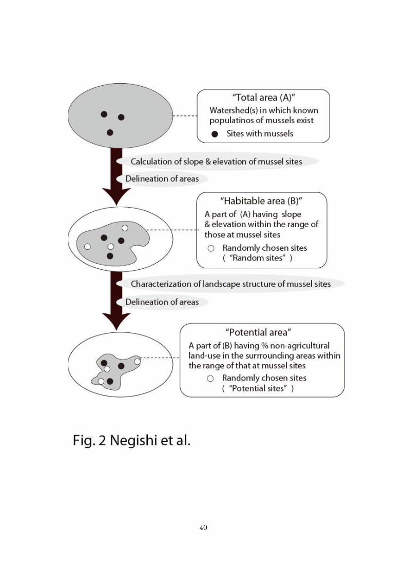
area of the three regions is hereafter referred to as the total area (Fig. 2). We recorded 139

the geographical locations of the mussel sites using GPS (CS60, Garmin Co., USA) and 140

registered on GIS (Arcmap, ver. 9.3, ESRI Co., USA). Using the surface elevation 141

distribution (50-m resolution, Geospatial Information Authority of Japan), a digital 142

elevation model (DEM) was generated. A ground surface slope distribution model 143

(50-m resolution; DSM) was also created based on DEM. We calculated the average 144

elevation and slope of each site by calculating average DEM and DSM values within 145

the 100-m radius buffer polygon surrounding each site. We carefully examined the data 146

and excluded the slope values where the 100-m buffer polygon enclosed unusual 147

topographic variations such as adjacent hill slopes because the DSM was particularly 148

sensitive to such errors (this occurred at five sites). Channel slope can limit mussel 149

distribution by potentially mediating hydraulic forces on the benthic habitat conditions 150

10

(Arbuckle and Downing 2002). Temperature can also limit mussel distribution because 151

of the physiological thermal tolerance of mussels and/or that of their host fish species 152

whose distribution can determine the distribution of mussels (Galbraith et al. 2010; 153

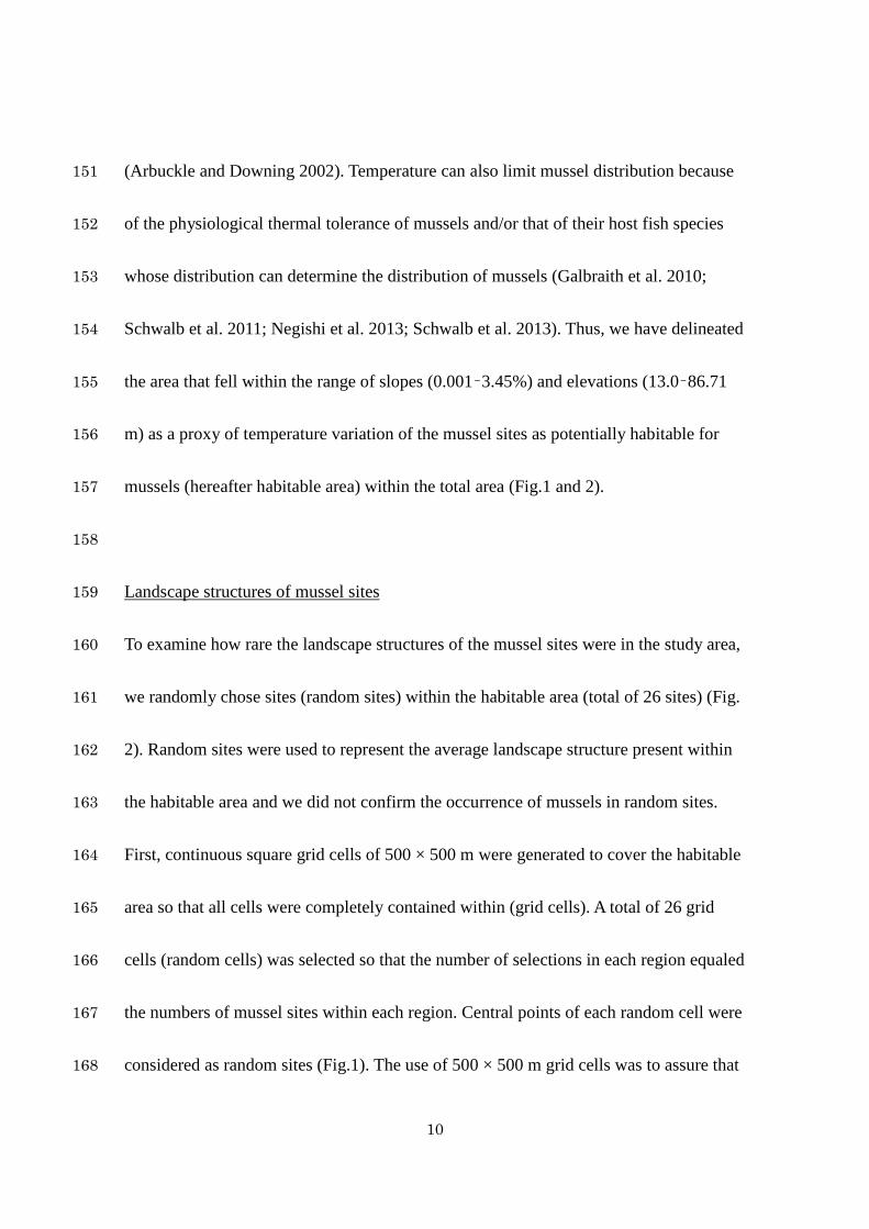
Schwalb et al. 2011; Negishi et al. 2013; Schwalb et al. 2013). Thus, we have delineated 154

the area that fell within the range of slopes (0.001–3.45%) and elevations (13.0–86.71 155

m) as a proxy of temperature variation of the mussel sites as potentially habitable for 156

mussels (hereafter habitable area) within the total area (Fig.1 and 2). 157

158

Landscape structures of mussel sites 159

To examine how rare the landscape structures of the mussel sites were in the study area, 160

we randomly chose sites (random sites) within the habitable area (total of 26 sites) (Fig. 161

2). Random sites were used to represent the average landscape structure present within 162

the habitable area and we did not confirm the occurrence of mussels in random sites. 163

First, continuous square grid cells of 500 × 500 m were generated to cover the habitable 164

area so that all cells were completely contained within (grid cells). A total of 26 grid 165

cells (random cells) was selected so that the number of selections in each region equaled 166

the numbers of mussel sites within each region. Central points of each random cell were 167

considered as random sites (Fig.1). The use of 500 × 500 m grid cells was to assure that 168

11

randomly selected sites were apart from each other and from mussel sites at least by 169

800-m channel length (i.e., minimum distances among mussel sites). 170

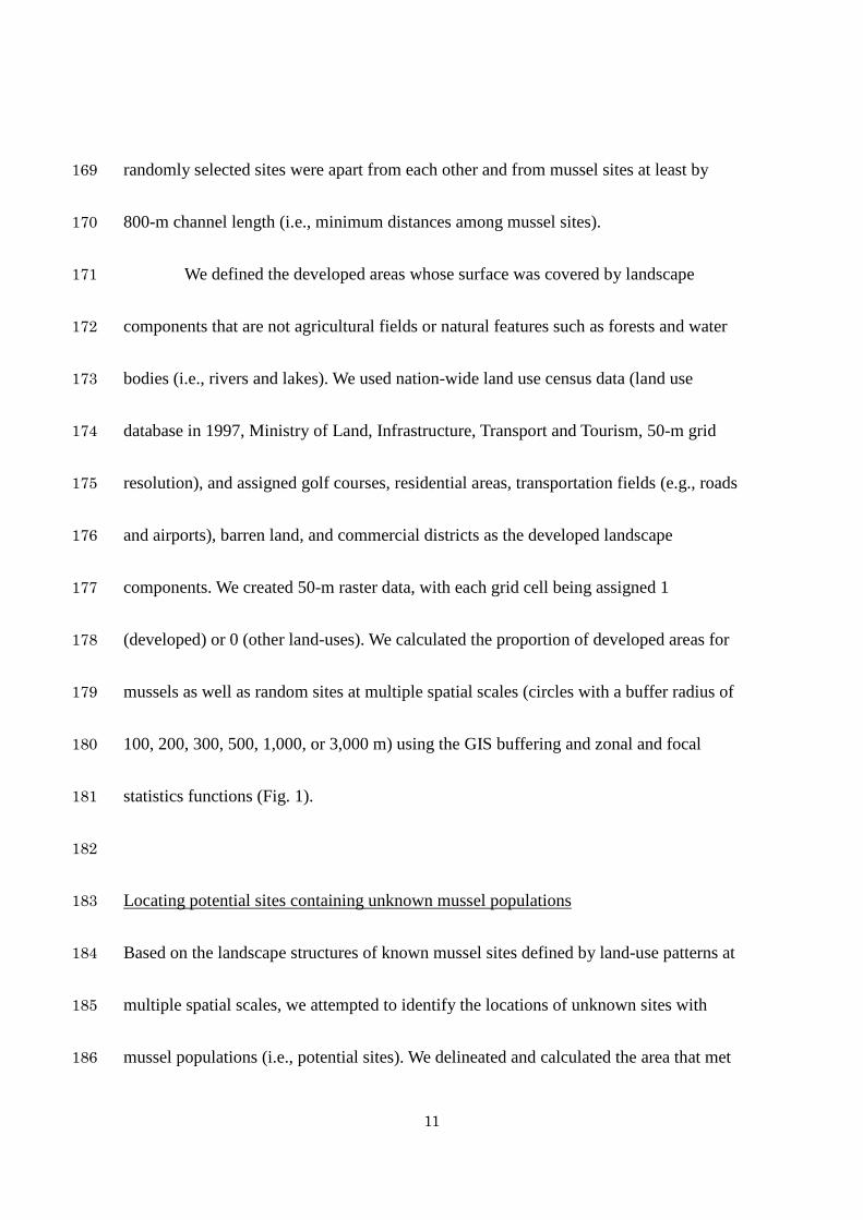
We defined the developed areas whose surface was covered by landscape 171

components that are not agricultural fields or natural features such as forests and water 172

bodies (i.e., rivers and lakes). We used nation-wide land use census data (land use 173

database in 1997, Ministry of Land, Infrastructure, Transport and Tourism, 50-m grid 174

resolution), and assigned golf courses, residential areas, transportation fields (e.g., roads 175

and airports), barren land, and commercial districts as the developed landscape 176

components. We created 50-m raster data, with each grid cell being assigned 1 177

(developed) or 0 (other land-uses). We calculated the proportion of developed areas for 178

mussels as well as random sites at multiple spatial scales (circles with a buffer radius of 179

100, 200, 300, 500, 1,000, or 3,000 m) using the GIS buffering and zonal and focal 180

statistics functions (Fig. 1). 181

182

Locating potential sites containing unknown mussel populations 183

Based on the landscape structures of known mussel sites defined by land-use patterns at 184

multiple spatial scales, we attempted to identify the locations of unknown sites with 185

mussel populations (i.e., potential sites). We delineated and calculated the area that met 186

12

the landscape structure criteria for the mussel sites at respective spatial scales; the 187

criteria were set at 95% confidence intervals of the means of the proportion of the 188

developed area for mussel sites. We determined the area that met the criteria of each 189

spatial scale, as well as all spatial scales (i.e., potential areas) from the habitable area 190

using the GIS focal statistics function. For example, the potential area constrained by 191

criteria at all spatial scales refer to the area, any given locations within which had the 192

proportion of developed land in surrounding areas within the criteria for mussel sites at 193

all spatial scales examined (Fig. 2). 194

We excluded habitable areas in Mie prefecture (see Fig. 1) from the further 195

analyses because distant locations rendered frequent visiting for observations and 196

sampling impractical. We initially attempted to randomly choose candidates for 197

potential sites within the potential area as was done for the selection of random sites 198

using the 500 m grid cells; the selected cells were referred to as candidate cells. We 199

chose 18 candidate cells, the number same as that of initially designated mussel sites. 200

However, preliminary analyses revealed that the number of cells meeting such criteria 201

was too small (< 10 cells) to conduct a random selection (see results for more detail). As 202

an alternative, we selected cells based on the criteria set based on the maximum value of 203

the proportion of developed area at a spatial scale of 500 m (53.8%), which provided > 204

13

100 cells. When randomly chosen 18 candidate cells were placed on areas dominated by 205

large rivers (> 90%), or the areas without noticeable agricultural drainage channel 206

networks, candidate cells were re-chosen by a random selection procedure (this 207

occurred once). 208

209

Mussel and fish surveys 210

Fish and mussel communities were surveyed in the summer period between 8th and 13th 211

August when flow is stable and no noticeable precipitation was recorded in the 212

preceding 2 weeks. In the water management cycles for rice cultivation in the area, this 213

period typically provides the largest amount of water within the channel (Negishi et al. 214

2013). The exact locations of the potential sites within candidate cells were determined 215

as follows: The geographical coordinates for the central points of chosen grid cells were 216

determined by GIS and located in the field by GPS. The sampling sites were chosen by 217

the following criteria: Upon arrival at the location, the closest drainage channel was 218

located. The site suitability was confirmed when it was for drainage or 219

irrigation/drainage purpose(s), had decent water quality and perennial flow, and was of a 220

comparable size to that of the mussel sites. The presence of perennial flow with decent 221

water quality was confirmed by the occurrence of freshwater Mollusca such as 222

14

Pleuroceridae sp. and Viviparidae sp. Only those whose wetted channel width was 223

within the range of that in the mussel sites were selected. When the closest one did not 224

meet these criteria, the next closest ones were progressively examined until the criteria 225

were met. 226

At each study site, two sections having a longitudinal length 10 times the 227

average wetted surface width (range = 45–320 cm) were set for mussel surveys with a 228

distance of 20 times the width between each section. In each section, electrical 229

conductivity (EC), pH, and water temperature (°C) were recorded using a 230

multi-parameter water quality probe (WM-22EP; DKK-TOA Co., Japan). Mussels were 231

quantified by collecting all mussels within the belt transects (a dimension of 25 × the 232

wetted channel width) equally spaced along a longitudinal profile. The total number of 233

transects was proportional to the section length (n = 4–32) and total areas searched 234

ranged from 0.9 to 36.8 m2. Mussels were collected by thoroughly sieving the sediment 235

using baskets (1-cm mesh), identified, enumerated, and measured along their longest 236

shell axes. Fish communities were surveyed by enclosing a section (20 times the length 237

of the wetted width) in the area upstream of the mussel survey sections. To avoid 238

disturbing the fish communities, the survey was conducted prior to the mussel survey. 239

Fish were caught by conducting two passes of catches using triangular scoop nets 240

15

(34-cm wide and 33-cm high mouth opening; 44-cm long; 2-mm mesh) aligned 241

perpendicularly to the channel. Furthermore, specific areas such as those with a fast 242

current and along the channel edge were thoroughly searched for fishes using scoop nets 243

(up to 5 min by two or three personnel depending on the channel size). Fish were 244

identified, enumerated, and photographed to digitally estimate their body sizes. 245

Collected organisms were released back to the capture area immediately after the 246

measurements had been taken. 247

248

Statistical analyses 249

Repeated measures two-way analysis of variance (ANOVA) was conducted to examine 250

the effects of spatial scale and site characteristics (mussel sites vs. random sites, or 251

mussel sites vs. potential sites), and their interactions on the proportion of developed 252

areas in surrounding areas. Site identity was included as a repeated measures factor. 253

When significant interaction terms were detected, the proportion of developed lands was 254

compared between site types at each scale using Student's t-tests. A correlogram of 255

Moran’s I was constructed to assess the degree of spatial autocorrelation in the 256

presence/absence data obtained from field surveys on mussels; presence data from 257

present sites (initially designated mussel sites in addition to some potential sites with 258

16

mussel populations) whereas absence data from absent sites (remaining potential sites 259

without mussels). Environmental variables (GIS-calculated elevation and slope, water 260

temperature, pH, EC, and flow rate) were compared between present and absent sites 261

using Welch’s t-tests. Fish community metrics were calculated as abundance, taxonomic 262

richness, and Shannon-Wiener index. These fish metrics, calculated for both 263

communities, included all taxa and those excluding bitterlings; bitterlings require live 264

mussels for spawning (Negishi et al. 2013). Mussel community metrics were calculated 265

with the pooled data from two sections in terms of abundance and mussel taxonomic 266

richness. Fish and mussel abundance were expressed as density (the number of 267

individuals either per 1 m2 or 100 m2). Mussel indicator roles were examined in two 268

ways. First, fish community metrics were compared between present and absent sites 269

using Welch’s t-tests. Second, relationships between mussel and fish community metrics 270

were examined by regression analysis (12 cases in total) with the former as independent 271

and the latter as dependent variables. All statistical analyses were conducted in R 2.10.1 272

(R Development Core Team, 2008) with a significance level of 0.05. The Bonferroni 273

correction was applied to the statistical significance level when appropriate. 274

275

Results 276

17

The change pattern of the proportions of developed lands in the surrounding areas in 277

response to variable spatial scales differed between the sites with known mussel 278

populations and those of randomly chosen sites (interaction effect: F5, 245= 6.8, p < 279

0.001). The differences in landscape structures between two types of sites were 280

particularly high at relatively small spatial scales (Fig. 3A). The proportions of 281

developed lands were significantly lower for the sites with known mussel populations 282

compared with those of randomly chosen sites (site effect: F1, 49 = 12.22, p < 0.001; Fig. 283

3A). The proportions of developed lands were significantly lower at sites with mussels 284

at the spatial scales of 100, 200, and 300 m when compared at respective spatial scales 285

(Fig. 3A). 286

The areal extent of lands (potential areas) that fell within the landscape 287

conditions of mussel sites at different spatial scales became disproportionately less with 288

decreasing spatial scale (Table 1). Approximately 7% of the total area was selected as 289

within the slope and elevation range of sites with existing mussel populations (habitable 290

area). The areal extent of the potential area that met the landscape-level criteria of 291

mussel sites across all spatial scales only constituted 0.23% of the habitable area. The 292

potential sites, which were selected based on the criteria of maximal areal proportion of 293

developed land at a scale of 500 m (53.8%), had landscape structures similar to those of 294

18

mussel sites (Fig. 3B). The change pattern of the proportions of developed lands in the 295

surrounding areas in response to variable spatial scales did not differ between two types 296

of sites (interaction effect: F5, 165 = 0.17, p = 0.97). The potential sites had a proportion 297

of developed lands similar to that of mussel sites in surrounding area (site effect: F1, 33 = 298

1.16, p = 0.29; Fig. 3B) with a significant effect of spatial scale (F5, 165 = 18.84, p < 299

0.001). 300

In total, 2, 128 individuals were found: 1, 764 P. japanensis, 118 L. grayana, 301

56 O. omiensis, 78 Inversidens brandti, 107 Anodonta spp., and 5 U. douglasiae 302

nipponensis. We found mussels in three out of 18 potential sites (at least one live 303

individual in the quadrat survey) (Fig. 4A). A clear spatial structure was revealed in the 304

distribution of present and absent sites with Moran’s correlogram indicating statistically 305

significant positive autocorrelation for small-distance categories (Fig. 4B). It is 306

important to note that three potential sites with mussels were close to each other or close 307

to the sites with known mussel populations, augmenting the patchy distribution. Sites 308

with mussels (including the three potential sites with mussels) and those without 309

mussels were similar to each other in the measured environmental variables (Table 2). 310

Mean (±SD) mussel density (individuals/m2), irrespective of taxon, at sites with mussel 311

populations was 29.6 (±57.3) individuals/m2. In total, 2,390 fish, consisting of 24 taxa, 312

19

were collected (Appendix); their body length was <15 cm. When compared between 313

sites with and without mussels, fish species richness with all taxa included and taxa 314

excluding bitterling species were both higher at the sites with mussels compared with 315

those without (Fig. 5; p < 0.001). The Shannon-Wiener index did not differ among site 316

type (p > 0.20). Mussel taxonomic richness was positively associated with fish species 317

richness (both with and without bitterlings) and the Shannon-Wiener index calculated 318

from all taxa included (Fig. 6). Mussel abundance did not have any predictive effect on 319

fish community metrics (p > 0.12). 320

321

Discussion 322

We demonstrated that the landscape structure surrounding agricultural drainage 323

channels with imperiled unionoid mussels was characterized by rural landscapes having 324

a significantly lower level of land development compared with common landscapes in 325

the area with similar elevation and slope ranges. This difference was more pronounced 326

when landscape structure was examined at relatively small spatial scales. These results 327

agree with our prediction that mussel habitats possess relatively rare rural landscape 328

features in the region. The interpretation of our findings requires caution because we did 329

not compare landscape structures between the sites with and without mussels. Also, we 330

20

did not constrain our analyses to the areas where only the landscape structures varied, 331

with other important factors (see the next paragraph) being more or less controlled when 332

selecting random sites. 333

The absence of GIS-ready digital data resources of drainage channel networks 334

across a large area prevented us from taking into the account spatial attributes of 335

drainage channel networks when delineating areas potentially suitable as mussel habitat. 336

For example, drainage density (i.e., total length of channels in a given unit area; see 337

Benda et al. 2004), which is analogous to habitat availability, could have been 338

particularly meaningful. Thus, it is possible that some of the random sites were selected 339

from areas where highly urban landscapes dominated and as a result few drainage 340

channels existed (relatively low habitat availability). Consequently, the differences in 341

landscape structure between the mussel and random sites can be partly a reflection of 342

the differences in land-use patterns (rural vs. urban) and not necessarily those around 343

drainage channels. Despite such limitations, the results implied that a quantitative 344

measure of rare landscape structure is useful when narrowing down the areas where 345

mussel habitat likely to occur. 346

We showed that areas with landscape structures characteristic of mussel sites 347

across multiple spatial scales constituted only a fraction of habitable area in the region 348

21

(0.23%) and was much less when compared with the areas estimated at respective 349

spatial scales (Table 2). This suggests that mussel sites can be more accurately defined 350

by considering landscape metrics quantified at multiple spatial scales. Our findings 351

underscore the importance of considering landscape structures at multiple spatial scales 352

when explaining organism distribution patterns (also see Marchand 2004; Stephens et al. 353

2004). Furthermore, landscape structure characteristic of mussel sites were more 354

pronounced and became rarer at relatively small spatial scales. Cao et al. (2013) 355

examined the relationships between landscape metrics and riverine mussel habitat 356

conditions and also reported the disproportionately strong influences of landscape 357

conditions in a close proximity (i.e., riparian zone). In the study region, the increase of 358

developed land surface within the area in a relatively short distance from mussel sites 359

likely causes a disproportionately large drop in potential habitat availability and may 360

degrade mussel habitat quality more severely. 361

Unknown mussel populations were found at only a few potential sites (16.7%), 362

indicating limited usefulness of landscape structure as a single predictor of mussel 363

habitat distribution. A patchy distribution of sites with mussels was apparent, and an 364

understanding and incorporation of its cause can improve the predictive model of 365

mussel distribution. Patchy distribution of mussels (mussel beds) is relatively well 366

22

reported at within-channel scales as well as at broader regional to continental scales 367

(Vaughn and Taylor, 2000; Strayer 2008). At larger scales, in particular, host fish species 368

distribution may be the one of the most important factors (Vaughn and Taylor 2000; 369

Schwalb et al. 2011). A patchy distribution can be caused by natural barriers (e.g., 370

drainage divide) for the dispersal of mussels (or host fish species), or as a result of 371

human-induced fragmentation and shrinkages of formerly broad distribution range 372

(Strayer 2008). Fish migrate up from rivers to drainage channels or rice paddies via 373

drainage channels seasonally (e.g., Katano et al. 2003). The placements of vertical drops 374

impassable for fish is common in modernized drainage channel networks (Miyamoto 375

2007). In agricultural channels, therefore, the reduction or loss of connectivity among 376

channels and/or between channels and downstream rivers might have fragmented 377

mussel habitat by limiting movement of host fish with attached glochidia. Other 378

potentially important factors on a local scale, such as flow velocity, hydraulic forces, 379

and physical channel structures, may also play a role in controlling the distribution of 380

mussels (Allen and Vaughn 2010; Matsuzaki et al. 2011; Nagayama et al. 2012; Negishi 381

et al. 2013). These factors independently or in a combination with other factors can 382

affect habitat conditions of mussels directly or indirectly by limiting distribution of host 383

fish species. Future studies should examine the relative importance of multiple factors 384

23

such as habitat fragmentation and local habitat conditions in relation to natural dispersal 385

ranges of host fish species (Schwalb et al. 2011; Cao et al. 2013; Schwalb et al. 2013). 386

Fish species richness was higher at sites with mussels compared to sites 387

without mussels despite of similar physico-chemical habitat conditions. This is 388

consistent with the findings that the occurrence of mussels is associated with the 389

presence of relatively species-rich fish communities (e.g., Vaughn and Taylor, 2000; 390

Negishi et al. 2013). Mussel species such as I. brandti, O. omiensis, and P. japanensis 391

co-occur with bitterlings through host-parasite relationships (Kitamura 2007; Terui et al. 392

2011). Importantly, when the bitterlings were removed, significant differences in fish 393

community species richness remained. This implies that the greater fish species richness 394

observed in the mussel sites was not the sole consequence of the addition of species 395

having a commensal relationship with mussels, but also several other ecological 396

processes (Negishi et al. 2013). Furthermore, the mussel taxonomic diversity gradient 397

predicted fish community taxonomic richness with mussels and the Shannon-Wiener 398

index relatively well. We previously tested fish and mussel communities in a <100 m2 399

area including some of the mussel sites used in the present study and reported the 400

relationships between fish and mussel community structure in different seasons (Negishi 401

et al. 2013). A discrepancy with the present study is that Negishi et al. (2013) reported 402

24

less explanatory power of mussels for fish community structure in the summer period. A 403

cause of such a discrepancy may be scale-dependent relationships between community 404

structure of fish and mussels (e.g., Schwalb et al. 2013). The mechanisms between 405

species richness and fish community structure also merit future research. We argue that 406

unionid mussel can be used as an indicator of fish habitat quality over a large scale (> 407

10,000 km2) at least within the area having elevation and slope ranges of mussel sites. 408

Our overall findings suggest that the quantitative measures of landscape 409

structure may serve as a useful tool when prioritizing or identifying areas for 410

conservation of mussels and fish if spatially auto-correlated distribution of habitat and 411

other critical environmental factors such as local habitat quality and habitat connectivity 412

are also considered. It is important to recognize the landscape structure in rural 413

landscape has changed in recent decades largely because of abandonment of agricultural 414

lands and land development associated with urbanizations (Nakamura and Short 2001; 415

Fujihara et al. 2005). Therefore, the landscape criteria quantified in the present study 416

should not be taken as an ideal habitat condition for mussels. Information on historical 417

distribution of mussels and land-use changes across a large area would provide crucial 418

insights into optimal habitat condition for mussels. 419

420

25

Acknowledgements 421

Members of Gifu–Mino Ecological Research Group, in particular Y. Miwa and K. 422

Tsukahara, provided logistical supports in the field. J Kitamura of (Mie Prefectural 423

Museum provided us information on mussel habitat. We are also indebted to two 424

anonymous reviewers whose comments greatly improved the paper. We thank Global 425

COE program of MEXT at Hokkaido University and the Ministry of Environment, 426

Japan for funding the research. This work was also supported by Grant-in-Aid for 427

Young Scientists (B) to JNN (24710269). 428

429

References 430

Allen DC, Vaughn CC (2010) Complex hydraulic and substrate variables limit 431

freshwater mussel species richness and abundance. J N Am Benthol Soc 29: 432

383-394 433

Aldridge DC, Fayle TM, Jackson N (2007) Freshwater mussel abundance predicts 434

biodiversity in UK lowland rivers. Aquat Conserv 17:554-564 435

Arbuckle KE, Downing JA (2002) Freshwater mussel abundance and species richness: 436

GIS relationships with watershed land use and geology. Can J Fish Aquat Sci 437

59:310-316 438

26

Armitage PD, Szoszkiewicz K, Blackburn JH, Nesbitt I (2003) Ditch communities: a 439

major contributor to floodplain biodiversity. Aquat Conserv 13:165-185 440

Benda L, Poff NL, Miller D, Dunne T, Reeves G, Pess G, Pollock M (2004). The 441

network dynamics hypothesis: how channel networks structure riverine habitats. 442

BioScience 54:413-427 443

Biggs J, Williams P, Whitfield M, Nicolet P, Brown C, Hollis J, Arnoldd D, Pepperd T 444

(2007) The freshwater biota of British agricultural landscapes and their 445

sensitivity to pesticides. Agr Ecosyst Environ 122:137-148 446

Cao Y, Huang J, Cummings KS, Holtrop A (2013). Modeling changes in freshwater 447

mussel diversity in an agriculturally dominated landscape. Freshwater Science 448

32:1205-1218 449

Daniel WM, Brown KM (2013) Multifactorial model of habitat, host fish, and landscape 450

effects on Louisiana freshwater mussels. Freshw Sci 32:193-203 451

Elphick CS (2000) Functional equivalency between rice fields and seminatural wetland 452

habitats. Conserv Biol 14:181-191 453

Fujihara M, Hara K, Short KM (2005) Changes in landscape structure of “yatsu” 454

valleys: a typical Japanese urban fringe landscape. Landscape Urban Plan 455

70:261-270 456

27

Galbraith HS, Spooner DE, Vaughn CC (2010) Synergistic effects of regional climate 457

patterns and local water management on freshwater mussel communities. Biol 458

Conserv 143: 1175-1183 459

Gergel SE, Turner MG, Miller JR, Melack JM, Stanley EH (2002) Landscape indicators 460

of human impacts to riverine systems. Aquat Sci 64:118-128 461

Herzon I, Helenius J (2008) Agricultural drainage ditches, their biological importance 462

and functioning. Biol Conserv 141:1171-1183 463

Janse JH, Peter JTM, Puijenbroek V (1998) Effects of eutrophication in drainage 464

ditches. Environ Pollut 102:547-552 465

Katano O, Hosoya K, Iguchi KI, Yamaguchi M, Aonuma Y, Kitano S (2003) Species 466

diversity and abundance of freshwater fishes in irrigation ditches around rice 467

fields. Environ Biol Fish 66:107-121 468

Katoh K, Sakai S, Takahashi T (2009) Factors maintaining species diversity in 469

satoyama, a traditional agricultural landscape of Japan. Biol Conserv 470

142:1930-1936 471

Kitamura J (2007) Reproductive ecology and host utilization of four sympatric bitterling 472

(Acheilognathinae, Cyprinidae) in a lowland reach of the Harai River in Mie, 473

Japan. Envion Biol Fish 78:37-55 474

28

Lydeard C, Cowie RH, Ponder WF, Bogan AE, Bouchet P, Clark SA, Cummings KS, 475

Frest TJ, Gargominy O, Herbert DG, Hershler R, Perez KE, Roth B, Seddon M, 476

Strong EE, Thompson FG (2004) The global decline of nonmarine mollusks. 477

BioScience 54:321-330 478

Marchand MN (2004) Effects of habitat features and landscape composition on the 479

population structure of a common aquatic turtle in a region undergoing rapid 480

development. Conserv Biol 18:758-767 481

Matsuzaki SS, Terui A, Kodama K, Tada M, Yoshida T, Washitani I (2011) Influence 482

of connectivity, habitat quality and invasive species on egg and larval 483

distributions and local abundance of crucian carp in Japanese agricultural 484

landscapes. Biol Conserv 144:2081-2087 485

Miyamoto K (2007) Harmonization of irrigation system development and ecosystem 486

preservation in paddy fields. Paddy Water Environ 5:1-4 487

Moilanen A, Wilson KA (2009) Spatial conservation prioritization : quantitative 488

methods and computational tools. Oxford University Press, Oxford [etc.]. 489

Morales Y, Weber LJ, Mynett AE, Newton TJ (2006) Effects of substrate and 490

hydrodynamic conditions on the formation of mussel beds in a large river. J N 491

Am Benthol Soc 25:664-676 492

29

Nagayama S, Negishi JN, Kume M, Sagawa S, Tsukahara K, Miwa Y, Kayaba Y 493

(2012) Habitat use by fish in small perennial agricultural canals during 494

irrigation and non-irrigation periods. Ecol Civil Eng 15:147-160 (in Japanese 495

with English abstract) 496

Nakamura T, Short K (2001). Land-use planning and distribution of threatened wildlife 497

in a city of Japan. Landscape Urban Plan 53:1-15 498

Natuhara Y (2012) Ecosystem services by paddy fields as substitutes of natural 499

wetlands in Japan. Ecol Eng 56:97-106 500

Negishi JN, Kayaba Y (2009). Effects of handling and density on the growth of the 501

unionoid mussel Pronodularia japanensis. J N Am Benthol Soc 28:821-831 502

Negishi JN, Kayaba Y, Tsukahara K, Miwa Y (2008) Towards conservation and 503

restoration of habitats for freshwater mussels (Unionoida). Ecol Civil Eng 504

11:195-211. (in Japanese with English abstract) 505

Negishi JN, Nagayama S, Kume M, Sagawa S, Kayaba Y, Yamanaka Y (2013) 506

Unionoid mussels as an indicator of fish communities: A conceptual framework 507

and empirical evidence. Ecol Indic 24:127-137 508

Onikura N, Nakajima J, Eguchi K, Inui R, Higa E, Miyake T, Kawamura K, Matsui S, 509

Oikawa S (2006) Changes in distribution of bitterlings, and effects of 510

30

urbanization on populations of bitterlings and unionid mussels in Tatara River 511

System, Kyusyu, Japan. J Jpn Soc Water Environ 29:837-842 (in Japanese with 512

English abstract) 513

R Development Core Team (2008) R: a language and environment for statistical 514

computing. R Foundation for Statistical Computing, Vienna, Austria. 515

Sato H (2001) The current state of paddy agriculture in Japan. Irrig Drain 50:91-99 516

Schwalb AN, Cottenie KARL, Poos MS, Ackerman JD (2011). Dispersal limitation of 517

unionid mussels and implications for their conservation. Freshw Biol 518

56:1509-1518 519

Schwalb AN, Morris TJ, Mandrak NE, Cottenie K (2013) Distribution of unionid 520

freshwater mussels depends on the distribution of host fishes on a regional scale. 521

Divers Distrib 19:446–454 522

Stephens SE, Koons DN, Rotella JJ, Willey DW (2004) Effects of habitat fragmentation 523

on avian nesting success: a review of the evidence at multiple spatial scales. 524

Biol Conserv 115:101-110 525

Strayer DL (2008) Freshwater mussel ecology—a multi-factor approach to distribution 526

and abundance. University of California Press, Berkeley and Los Angeles. 527

Takahashi Y (1994) Characteristics of rice field irrigation: The Japanese experience. Int 528

31

J Water Resour D 10:425-430 529

Terui A, Shin-ichiro SM, Kodama K, Tada M, Washitani I (2011) Factors affecting the 530

local occurrence of the near-threatened bitterling (Tanakia lanceolata) in 531

agricultural canal networks: strong attachment to its potential host mussels. 532

Hydrobiologia 675:19-28 533

Vaughn CC, Taylor CM (2000) Macroecology of a host-parasite relationship. 534

Ecography 23:11-20. 535

Wang L, Lyons J, Kanehl P, Bannerman R (2001). Impacts of urbanization on stream 536

habitat and fish across multiple spatial scales. Environ Manage 28:255-266 537

Williams P (2004) Comparative biodiversity of rivers, streams, ditches and ponds in an 538

agricultural landscape in Southern England. Biol Conserv 115:329-341 539

Xu YJ, Wu K (2006) Seasonality and interannual variability of freshwater inflow to a 540

large oligohaline estuary in the Northern Gulf of Mexico. Estuaries Coast Shelf 541

S 68:619-626 542

32

Table 1: Areal extent of the potential area that met the criteria of mussel site landscape 543

structures at different spatial scales and their relative availability (%) relative to total 544

and habitable areas. For example, 7.41% of total area is considered suitable for mussel 545

habitat based on the range of elevation and slope of sites with mussels; 9.64% of the 546

habitable area was considered suitable for mussel habitat when considering landscape 547

structure obtained for the surrounding area of mussel sites at the scale of 100 m (the 548

area within a circular buffer having a radius of 100 m). 549

Area (km2) Availability (%)

Total area 6,399.32

Habitable area 473.89 7.41

3000-m buffer criteria 131.26 27.70*

1000-m buffer criteria 113.55 23.96*

500-m buffer criteria 97.68 20.61*

300-m buffer criteria 64.63 13.64*

200-m buffer criteria 58.24 12.29*

100-m buffer criteria 45.68 9.64*

Multiple-scale criteria 1.07 0.23*

* These values were calculated as a proportion relative to the habitable area 550

551

552

33

Table 2 General characteristics of study reaches with (present) and without (absent)

freshwater mussels. Means ± SD are shown. Statistical significance as the result of Weltch’s

t-tests are also shown; significance level is Bonferroni-corrected (p = 0.05/6).

†Sample size was 15 for slope as the 5 sites were excluded because of unusual land surface

slope was estimated due to the presence of steep hillslope near the channel.

Present (n=20†) Absent (n=15) Statistical significance

Elevation (m) 43.61±18.16 32.88±16.72 p = 0.08

Slope (%) 0.69±0.57 0.57±0.43 p = 0.67

Temp. (˚C) 27.45±2.10 26.42±1.35 p = 0.08

pH 7.12±0.69 7.80±0.62 p = 0.01

EC (µS/cm) 9.81±7.15 9.41±3.52 p = 0.83

Flow rate (m3) 0.19±0.31 0.15±0.11 p = 0.63

34

Appendix: Taxon list and general characteristics of fish communities in the study reaches.

Abundances for the sites with and without mussels are shown; mean ± SD (maximum values;

minimum values were all zero).

Family Species name Present (n = 20) Absent (n = 15)

Cyprinidae

Rhodeus ocellatus ocellatus 17.12±45.86 (194.44) 0 Tanakia lanceolata 35.81±94.88 (395.83) 0 Tanakia limbata 190.86±404.25 (1693.12) 0 Carassius sp. 6.43±18.00 (74.07) 2.22±8.31 (33.33) Nipponocypris sieboldii 85.78±173.04 (732.64) 40.30±150.77 (604.44) Nipponocypris temminckii 46.37±101.26 (324.79) 2.47±9.24 (37.04) Zacco platypus 6.82±23.67 (105.82) 10.15±21.54 (71.11) Abbottina rivularis 9.29±39.31 (180.56) 0 Gnathopogon elongatus 65.12±208.52 (958.33) 3.54±9.16 (30.86) Hemibarbus barbus 0 1.19±4.43 (17.78) Pseudogobio esocinus 4.83±11.91 (48.61) 0 Sarcocheilichthys

variegatus variegatus 0.17±0.76 (3.47) 0

Rhynchocypris logowskii

steindachneri 1.10±4.07 (18.52) 7.11±21.78 (86.42)

Rhynchocypris oxycephalus

jouyi 0.17±0.76 (3.47) 0

Pseudorasbora parva 4.08±16.63 (76.39) 0 Adrianichthyidae

Oryzias latipes 59.48±183.58 (833.33) 225.91±613.96 (2455.56) Cobitidae

Cobitis biwae 1.66±4.48 (15.87) 29.71±107.92 (433.33) Cobitis sp. 1.19±5.19 (23.81) 0 Misgurnus anguillicaudatus 63.48±103.56 (370.37) 109.06±199.33 (740.74) Paramisgurnus dabryanus 0 3.29±12.32 (49.38) Gobiidae

Rhinogobius sp. 42.67±36.65 (128.47) 75.64±134.90 (444.44) Odontobutidae

Odontobutis obscura 0.69±3.03 (13.89) 0 Petromyzontidae

35

Lethenteron reissneri 0 0.82±3.08 (12.35) Siluridae

Silurus asotus 0 0.46±1.73 (6.94)

36

Figure captions

Figure 1: Location of the study area (A), study sites where unionoid mussel

populations were present (mussel sites; n = 26) (B), an example of measurements of

landscape structure in relation to multiple buffers surrounding the study sites (C), an

example of the area potentially suitable as mussel habitat (habitable area; see the text

for details) shown in white within region A (D), and an example of sites with mussels

(mussel sites; filled circles) and sites randomly selected (random sites; open circles)

(E). The regions A, B, and C in (B) denote watersheds within which random site

selections were conducted. The sites enclosed with a broken line (n = 18) in (B) were

used when testing mussel/fish relationships. The gray areas in (C) and scratched area in

(E) denote the land use categorized as non-agricultural developed use such as urban

areas.

Figure 2: A diagram depicting the procedure of delineating total area, habitable area,

and potential area in association with sites with mussels (mussel sites), random sites,

and potential sites.

37

Figure 3: Means ± SE of proportion of developed non-agricultural areas surrounding

the study sites with mussels (mussel sites; filled circles) and randomly chosen sites

(random sites; open triangles) at different spatial scales of buffer radii used to calculate

landscape metrics. In (A), random sites (n = 26) were selected within the boundary of

several watersheds and the range of elevation and ground surface slopes for the mussel

sites (Fig. 1). In (B), the selection of potential sites (n = 18) was further constrained by

the range of landscape characteristics at the spatial scale of 500 m. Asterisks indicate

statistically significant pair-wise differences at respective spatial scales using Student's

t-tests with Bonferroni corrections (p = 0.05/6; p = 0.005).

Figure 4: Spatial distribution of sites with mussels (filled circles) and without mussels

(open circles) (A) and spatial correlogram of the occurrence (presence or absence) of

mussels, where the abscissa is distance classes and the ordinate Moran’s I coefficient

(B). In (A), three sites accompanied by arrow denote sites that were initially chosen as

potential sites and had mussel populations whereas the gray areas denote the habitable

area. **Significant with Bonferroni-corrected probability (p = 0.05/10; p = 0.005).

*Significant at the probability level p = 0.05 (i.e., before applying the Bonferroni

correction).

38

Figure 5: Box plots showing median (central thick lines), 25%, and 75% quartile

ranges around the median (box width) of taxonomic richness of fish community of all

data (A) and data excluding bitterling species (B) for sites with (present) and without

(absent) mussels. The sample size for each group was 21 and 15 for present and absent

sites, respectively. Only those with statistically significant differences are shown; the

statistical significance of Welch’s t-test was corrected with Bonferroni corrections (p =

0.05/6; p = 0.008).

Figure 6: Relationships between mussel taxonomic richness and fish community

metrics; Shannon-Wiener index of fish community (A), taxonomic richness of fish

community (B), and taxonomic richness of fish community of data excluding bitterling

species (C). Statistically significant regressions are shown as solid lines with

coefficients of determination (R2). Only those with statistically significant differences

regressions are shown; statistical significance levels were corrected with Bonferroni

corrections (p = 0.05/6; p = 0.008).

39

40

41

42

43

44