Impacts of Thinning on Carbon Stores in the PNW: A Plot ... · Impacts of Thinning on Carbon Stores...
72
Impacts of Thinning on Carbon Stores in the PNW: A Plot Level Analysis Joshua Clark, John Sessions, Olga Krankina, Thomas Maness Final Report College of Forestry Oregon State University 25 May 2011
Transcript of Impacts of Thinning on Carbon Stores in the PNW: A Plot ... · Impacts of Thinning on Carbon Stores...

i
Joshua Clark, John Sessions
Department of Forest Engineering, Resources and Management
College of Forestry
Oregon State University
22 October 2010
Impacts of Thinning on Carbon Stores in the PNW:
A Plot Level Analysis
Joshua Clark, John Sessions, Olga Krankina, Thomas Maness Final Report College of Forestry Oregon State University 25 May 2011

Impacts of Thinning – FINAL REPORT i
Table of Contents
Table of Figures ..................................................................................................................................................... iii
Table of Tables ....................................................................................................................................................... v
Executive Summary .............................................................................................................................................. vii
Introduction............................................................................................................................................................. 1
Model Overview ..................................................................................................................................................... 1
Thinning Prescriptions ....................................................................................................................................... 2
Choice of Model to Project Forest Carbon ........................................................................................................ 3
Carbon Fluxes .................................................................................................................................................... 3
Carbon Accounting Methods Used for this Report................................................................................................. 4
Carbon Store on Site ....................................................................................................................................... 4
Carbon Fluxes Directly from Thinning Scenarios .......................................................................................... 5
Carbon in harvested material .......................................................................................................................... 6
Carbon in wood products ................................................................................................................................ 7
Carbon in landfill ............................................................................................................................................ 7
Carbon in slash harvested and utilized as source for energy .......................................................................... 8
Avoided carbon emissions – comparison of carbon emissions between biomass and other energy sources . 8
Carbon emissions for Energy Alternative ...................................................................................................... 10
Life of Wood Products – Other Considerations ............................................................................................... 10
Other Carbon Fluxes ........................................................................................................................................ 10
Plot Selection ........................................................................................................................................................ 10
Dominant Tree Species for each Plot............................................................................................................... 10
Plot Understory Vegetation ............................................................................................................................. 11
Carbon Pool Estimates for Plots Prior to Treatment ........................................................................................ 11
Criteria for Stand Treatments ............................................................................................................................... 12
Thinning Strategies .......................................................................................................................................... 12
Light Thin....................................................................................................................................................... 12
“Breakeven” Thin ........................................................................................................................................... 12
Heavy Thin ..................................................................................................................................................... 12
Stand Treatment Considerations ...................................................................................................................... 12
Example Plot ......................................................................................................................................................... 13

Impacts of Thinning – FINAL REPORT ii
Torching and Crowning Index ......................................................................................................................... 14
Silvicultural Prescription and Carbon Effects .................................................................................................. 14
Harvesting System ........................................................................................................................................... 16
Costs ................................................................................................................................................................ 16
Wood Products ................................................................................................................................................. 17
Overall Cost/Revenue Analysis ....................................................................................................................... 18
Analysis ................................................................................................................................................................ 19
Results .................................................................................................................................................................. 20
Financial Sensitivity ........................................................................................................................................ 21
Potential Alternative Management for Younger Stands .................................................................................. 21
Other Carbon Fluxes ............................................................................................................................................. 22
Next Steps ............................................................................................................................................................. 22
Contact Information .............................................................................................................................................. 23
References............................................................................................................................................................. 24
Appendix A. Coordinates of Plots for each County ............................................................................................. 31
Appendix B. Stand Level Characteristics for each Plot, by County ..................................................................... 34
Appendix C. Understory Vegetation by County ................................................................................................... 39
Appendix D. Detailed Carbon Simulations, Grouped by Age, Region and Thinning……………………….… . 44
Appendix E. Carbon Accounting Methodology Using FVS and other Tools……………………….… .............. 52
Appendix F. Summary Tables of Carbon Stores, Fluxes, Relative Carbon and Fuel Reduction Measurement ... 55
Appendix G. Conversion Units and Definitions……………………….… .......................................................... 61
Impacts of Thinning – FINAL REPORT iii
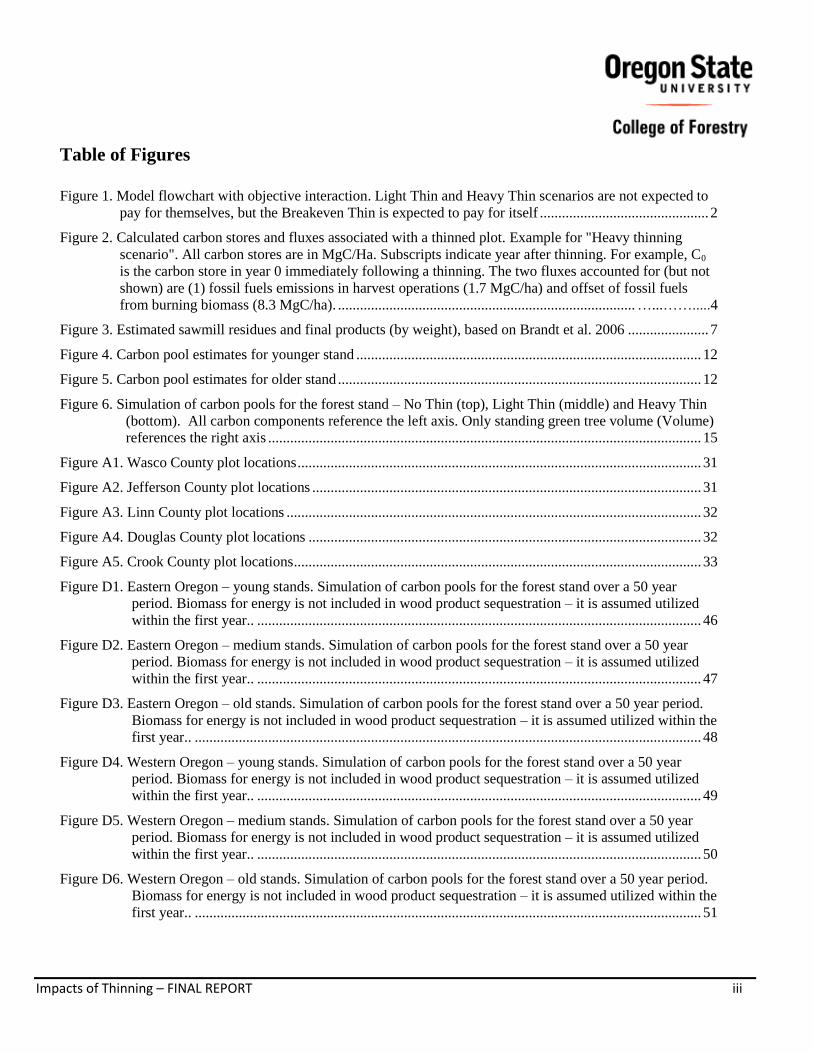
Table of Figures
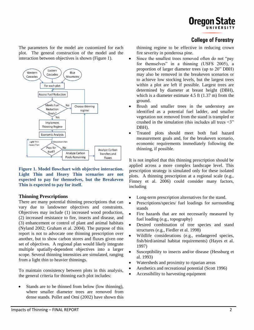
Figure 1. Model flowchart with objective interaction. Light Thin and Heavy Thin scenarios are not expected to
pay for themselves, but the Breakeven Thin is expected to pay for itself .............................................. 2
Figure 2. Calculated carbon stores and fluxes associated with a thinned plot. Example for "Heavy thinning
scenario". All carbon stores are in MgC/Ha. Subscripts indicate year after thinning. For example, C0
is the carbon store in year 0 immediately following a thinning. The two fluxes accounted for (but not
shown) are (1) fossil fuels emissions in harvest operations (1.7 MgC/ha) and offset of fossil fuels
from burning biomass (8.3 MgC/ha). ................................................................................. …...…….....4
Figure 3. Estimated sawmill residues and final products (by weight), based on Brandt et al. 2006 ...................... 7
Figure 4. Carbon pool estimates for younger stand .............................................................................................. 12
Figure 5. Carbon pool estimates for older stand ................................................................................................... 12
Figure 6. Simulation of carbon pools for the forest stand – No Thin (top), Light Thin (middle) and Heavy Thin
(bottom). All carbon components reference the left axis. Only standing green tree volume (Volume)
references the right axis ...................................................................................................................... 15
Figure A1. Wasco County plot locations .............................................................................................................. 31
Figure A2. Jefferson County plot locations .......................................................................................................... 31
Figure A3. Linn County plot locations ................................................................................................................. 32
Figure A4. Douglas County plot locations ........................................................................................................... 32
Figure A5. Crook County plot locations ............................................................................................................... 33
Figure D1. Eastern Oregon – young stands. Simulation of carbon pools for the forest stand over a 50 year
period. Biomass for energy is not included in wood product sequestration – it is assumed utilized
within the first year.. ......................................................................................................................... 46
Figure D2. Eastern Oregon – medium stands. Simulation of carbon pools for the forest stand over a 50 year
period. Biomass for energy is not included in wood product sequestration – it is assumed utilized
within the first year.. ......................................................................................................................... 47
Figure D3. Eastern Oregon – old stands. Simulation of carbon pools for the forest stand over a 50 year period.
Biomass for energy is not included in wood product sequestration – it is assumed utilized within the
first year.. .......................................................................................................................................... 48
Figure D4. Western Oregon – young stands. Simulation of carbon pools for the forest stand over a 50 year
period. Biomass for energy is not included in wood product sequestration – it is assumed utilized
within the first year.. ......................................................................................................................... 49
Figure D5. Western Oregon – medium stands. Simulation of carbon pools for the forest stand over a 50 year
period. Biomass for energy is not included in wood product sequestration – it is assumed utilized
within the first year.. ......................................................................................................................... 50
Figure D6. Western Oregon – old stands. Simulation of carbon pools for the forest stand over a 50 year period.
Biomass for energy is not included in wood product sequestration – it is assumed utilized within the
first year.. .......................................................................................................................................... 51

Impacts of Thinning – FINAL REPORT iv
Figure F1. Torching index (mi/hr) over a 50-year period – comparison is for different treatments for region/age
combinations. This is a graphical representation of the means (averages) from Table F3, and does
not include variance, which is relatively high compared to the mean... ............................................ 58
Figure F2. Crowning index (mi/hr) over a 50-year period – comparison is for different treatments for region/age
combinations. This is a graphical representation of the means (averages) from Table F3, and does
not include variance, which is relatively high compared to the mean.. ............................................. 59
Impacts of Thinning – FINAL REPORT v
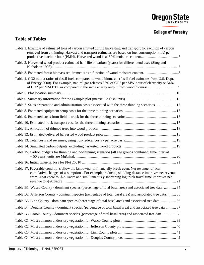
Table of Tables Table 1. Example of estimated tons of carbon emitted during harvesting and transport for each ton of carbon
removed from a thinning. Harvest and transport estimates are based on fuel consumption (lbs) per
productive machine hour (PMH). Harvested wood is at 50% moisture content. ....................................... 5
Table 2. Harvested wood product estimated half-life of carbon (years) for different end uses (Skog and
Nicholson 1998). ....................................................................................................................................... 7
Table 3. Estimated forest biomass requirements as a function of wood moisture content. .................................... 8
Table 4. CO2 output ratios of fossil fuels compared to wood biomass. (fossil fuel estimates from U.S. Dept.
of Energy 2000). For example, natural gas releases 38% of CO2 per MW-hour of electricity or 54%
of CO2 per MM BTU as compared to the same energy output from wood biomass.. .............................. 9
Table 5. Plot location summary ............................................................................................................................ 10
Table 6. Summary information for the example plot (metric, English units) ....................................................... 13
Table 7. Sales preparation and administration costs associated with the three thinning scenarios ...................... 17
Table 8. Estimated equipment setup costs for the three thinning scenarios ......................................................... 17
Table 9. Estimated costs from field to truck for the three thinning scenarios ...................................................... 17
Table 10. Estimated truck transport cost for the three thinning scenarios ............................................................ 17
Table 11. Allocation of thinned trees into wood products .................................................................................... 18
Table 12. Estimated delivered harvested wood product prices. ............................................................................ 18
Table 13. Total costs and revenues, using non-federal costs - per acre basis. ...................................................... 19
Table 14. Simulated carbon outputs, excluding harvested wood products ........................................................... 19
Table 15. Carbon budgets for thinning and no-thinning scenarios (all age groups combined; time interval
= 50 years; units are MgC/ha). ............................................................................................................ 20
Table 16. Initial financial loss for Plot 26510 ...................................................................................................... 21
Table 17. Favorable conditions allow the landowner to financially break even. Net revenue reflects
cumulative changes of assumptions. For example: reducing skidding distance improves net revenue
from -$503/acre to -$291/acre and simultaneously shortening log truck travel time improves net
revenue to -$201/acre ........................................................................................................................... 21
Table B1. Wasco County - dominant species (percentage of total basal area) and associated tree data. ............. 34
Table B2. Jefferson County - dominant species (percentage of total basal area) and associated tree data. ......... 35
Table B3. Linn County - dominant species (percentage of total basal area) and associated tree data. ................ 36
Table B4. Douglas County - dominant species (percentage of total basal area) and associated tree data. ........... 37
Table B5. Crook County - dominant species (percentage of total basal area) and associated tree data. .............. 38
Table C1. Most common understory vegetation for Wasco County plots ............................................................ 39
Table C2. Most common understory vegetation for Jefferson County plots ........................................................ 40
Table C3. Most common understory vegetation for Linn County plots ............................................................... 41
Table C4. Most common understory vegetation for Douglas County plots ......................................................... 42
Impacts of Thinning – FINAL REPORT vi
Table C5. Summary of understory vegetation variety for plots at the county level……………………...… ............... .43
Table D1. Classification of plots into two regions, six groups and twenty-four scenarios…………………………. .... 44
Table F1. Estimated mean carbon stores with associated standard error for each region/age category. Initial
growing stock volume is total volume, not merchantable volume. Carbon pools for each plot are
separated into three categories: (1) Live (Aboveground Standing, Belowground Live, Shrubs and Herbs);
(2) Dead (Belowground Dead, Standing Dead, Downed Dead Wood); and (3) Forest Floor. Data is
presented as: carbon mean [Mg/hectare] (carbon standard error) [Mg/hectare]…………………….…... 55
Table F2. Carbon pool estimate relative to initial carbon store where 100% is initial carbon store before
thinning………………………………………………………………………………………………… . .... .56
Table F3. Torching Index and Crowning Index estimates. Torching Index is the wind speed at which crown fire is
expected to initiate (based on Rothermel (1972) surface fire model and Van Wagner (1977) crown fire
initiation criteria). Crowning Index is the wind speed at which active crowning fires are possible (based
on Rothermel (1991) crown fire spread rate model and Van Wagner (1977) criterion for active crown
fire spread). Wind speed refers to speed of wind measured 20 ft above the canopy. Lower values
indicate higher susceptibility. Data is presented as: crowning/torching index [mi/hr] (standard
deviation) [mi/hr] for select years. Red indicates that plots would benefit from a thinning using the
criteria in this study. Orange indicates the average was still below criteria following the thinning, and
green indicates that the average index for plots was above the minimum criteria used in this study. .... ..... 57
Table F4. Number of plots within each region and age group with the greatest amount of Live, Dead, and Total
Carbon stores for each thinning scenario vs. no-thinning scenario. As seen in this table, carbon
stores in a plot following a thinning are always lower for every plot used in this analysis. ……………. ... 60
Impacts of Thinning – FINAL REPORT vii
Executive Summary
This report provides an analysis of forest carbon stores, fluxes and avoided emissions directly related to fuel reduction
thinnings for sample plots in eastern and western Oregon.
Primary Goals
Determine the level of on-site carbon storage under different thinning prescriptions and in different forest types.
Analyze plot-level forest carbon pools and carbon fluxes over a 50-year period. Compare alternative thinning
treatments with a no thinning scenario.
Estimate the amount of carbon transferred to harvested wood products, carbon emissions of biomass burning for
energy production, and avoided carbon emissions from not burning fossil fuels.
Determine if revenue from harvested wood products from the thinning treatment could pay for the thinning under
specified market and harvest unit assumptions for one thinning scenario (the “breakeven” scenario).
Methods
Plots were chosen from the Forest Inventory and Analysis (FIA) National Program and the Current Vegetation
Survey (CVS) to represent a range of common landscape types with stand conditions that show a potential for fuel
reduction.
Plots were all from Oregon, including the Eastern Cascade, Western Cascade, and Blue Mountain regions. A
wide range of stand ages was included (21-269 years for Eastern Oregon/Blue Mountains and 10-220 years for
Western Oregon).
Thinning scenarios were developed to meet specified torching and crowning thresholds. All simulated thinnings
use a “thin from below” (low thinning) approach. A control (no harvest scenario) is compared to different
treatments.
Carbon pools were estimated using the Fire and Fuels Extension (FFE) of the Forest Vegetation Simulator (FVS)
with manual adjustments and additions to address known model limitations.
Estimated harvest costs were based on the Fuel Reduction Cost Simulator (FRCS-West). Estimated timber
revenues were based on ODF data.
Findings
Forest carbon pools always immediately decreased as a result of a fuel reduction thinning, with larger differences
in total carbon pools resulting from heavier thinning treatments.
After thinning, forest carbon pools (both total and standing live aboveground) remain lower throughout a 50-year
period for all simulated plots in eastern and western Oregon. The difference in total carbon pools between a
thinned and unthinned plot is dependent on the level of live standing tree inventory reduction. A heavier thin
tends to reduce carbon pools more than lighter thins throughout a 50-year simulated period.
Carbon pool estimates for thinned stands were still lower than unthinned stands even after accounting for carbon
transfer to wood products and avoided emissions from fossil fuels for energy production. After simulating growth
Impacts of Thinning – FINAL REPORT viii
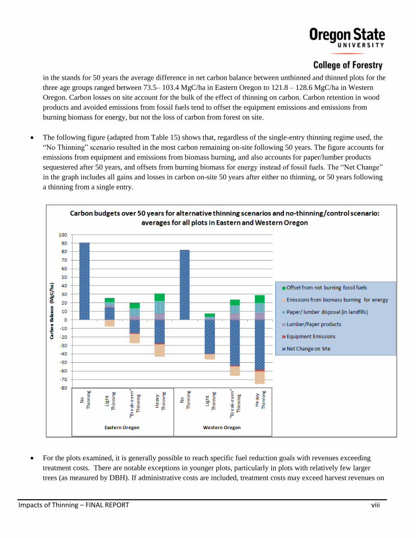
in the stands for 50 years the average difference in net carbon balance between unthinned and thinned plots for the
three age groups ranged between 73.5– 103.4 MgC/ha in Eastern Oregon to 121.8 – 128.6 MgC/ha in Western
Oregon. Carbon losses on site account for the bulk of the effect of thinning on carbon. Carbon retention in wood
products and avoided emissions from fossil fuels tend to offset the equipment emissions and emissions from
burning biomass for energy, but not the loss of carbon from forest on site.
The following figure (adapted from Table 15) shows that, regardless of the single-entry thinning regime used, the
“No Thinning” scenario resulted in the most carbon remaining on-site following 50 years. The figure accounts for
emissions from equipment and emissions from biomass burning, and also accounts for paper/lumber products
sequestered after 50 years, and offsets from burning biomass for energy instead of fossil fuels. The “Net Change”
in the graph includes all gains and losses in carbon on-site 50 years after either no thinning, or 50 years following
a thinning from a single entry.
For the plots examined, it is generally possible to reach specific fuel reduction goals with revenues exceeding
treatment costs. There are notable exceptions in younger plots, particularly in plots with relatively few larger
trees (as measured by DBH). If administrative costs are included, treatment costs may exceed harvest revenues on
Impacts of Thinning – FINAL REPORT ix
federal lands. Financial viability is significantly affected by many stand-dependent variables, including current
stand structure, average distance of wood from roadside, average distance of stand to mill/plant, and current
market prices.
Burning biomass from forest fuel reduction thinnings results in avoided carbon emissions from fossil fuels. Due
to relatively low energy density, biomass has greater carbon emissions from the boiler per energy unit produced
(CO2 emissions per kWh or BTU produced) when compared to carbon emissions from fossil fuels (coal, natural
gas) per energy unit produced.
All thinning scenarios on all plots without exception resulted in a significant loss of carbon relative to a no-
thinning scenario. This suggests that the findings may be applicable to other forest types and thinning
prescriptions.
Key Assumptions and Limitations
Our key assumption is that the life cycle analysis of carbon stores and fluxes begins with initial carbon
stores in the stand prior to thinning as described by Maness 2009. In other words, our analysis starts with
existing forest condition and measures the net change in carbon stores due to the thinning treatments. This
assumption contrasts with other studies (e.g., Lippke et al. 2004) that start with bare ground as a system
boundary. The results (and potentially the conclusions) can be dramatically affected by the choice of
system boundary.
Not considered in this analysis:
o Effects of fire on carbon pools and flux. This includes any potential post-thin treatments. In this
study, we do not estimate whether carbon emissions from prescribed fire and/or wildfire would (over
repeated cycles) be higher or lower after thinning.
o Soil carbon and fine roots (roots less than 2 mm in diameter).
o Emissions due to consumption of electric power in lumber and paper production. Including these
emissions would increase the greenhouse gas emissions for each of the thinning scenarios.
o Disposal methods for wood products (e.g., recycling and use as biofuel). In this analysis, wood
products are assumed either taken to a landfill or burned as an energy source.
o Effects of climate change (e.g., temperature, precipitation).
o Vegetation in-growth. This report assumes that in-growth is managed with regular treatment (e.g.,
with herbicides) that limits in-growth. If in-growth is allowed and fire is suppressed, estimates of
carbon pools on-site may significantly increase, especially for longer time periods.
o Emission reductions from substitution effects of wood products for more energy intensive alternative
building materials (such as concrete, brick, or steel). Inclusion of substitution effects would decrease
carbon emissions for thinning scenarios.
Because this is a plot-level study, where plots were chosen based on specific criteria (stand age, specific stand
structures, specific dominant species), study results cannot be extrapolated directly to a regional analysis.
The analysis assumes that there is no re-entry onto the site in the next 50 years. The stand projection is shown
for illustrative purposes only; it is not intended to be a management prescription.
Impacts of Thinning – FINAL REPORT x
Future Work
There are several potential areas of study that can support and enhance work begun in this report. This would close
the gap on some of the limitations presented within this report.
An expanded analysis would improve regional understanding of forest carbon stores in varying conditions. Inclusion
of one or more of the following variables would not only expand the scope of this report but also enhance the results
presented from the study.
Effects of prescribed fire and wildfire intensity and frequency on carbon stores.
Effects of strategic placement of thinning on carbon stores for larger areas.
o Effects of thinning in easily accessible areas (e.g., near roads) vs. thinning over larger areas.
o Urban thinning.
Effects of varying the price for biomass.
o Sensitivity analysis of biomass price (and potential impact of financial subsidies on thinning regime).
Inclusion of thinning regimes as part of a broader strategy to improve forest health or in response to
insects/disease (e.g., beetle kill).
Establish a more detailed time profile of carbon. This would include an annual carbon budget over a given
time frame instead of a carbon budget at less frequent intervals.
Since all thinning treatments reduced carbon storage over a 50-year period, it is possible that additional
entries would further reduce carbon stores. In order to more fully understand the effects, a more complete
forest management should be included in future work, instead of a single management action (thinning).
Joshua Clark
John Sessions
Olga Krankina
Thomas Maness
College of Forestry
Oregon State University, Corvallis, OR
Impacts of Thinning – FINAL REPORT 1
Introduction There is growing interest in improving the resilience of
forests to fire, insects, and disease in the Pacific
Northwest and in biomass recovery for energy
production (Graham et al. 2004; Lord et al. 2006). There
has also been extensive analysis and discussion on the
impact of forest management (and other disturbances) on
forest carbon stores and fluxes (Krankina and Harmon
2006). Other studies have developed regional estimates
of forest carbon stores (Dushku et al. 2007).
The purpose of this study is to determine the level of on-
site carbon stores at a plot level under different fuel
reduction thinning operations in different forest types in
Oregon. Some off-site carbon estimates are made as
well. A collection of relatively densely stocked plots was
chosen from five Oregon counties in the Western and
Eastern Cascades, southwest Oregon, and the Blue
Mountains region.
The carbon pools of each plot for thinned and unthinned
scenarios are projected and compared. The resulting
simulated carbon stores and carbon fluxes from this
model are not intended to be extrapolated to regional or
landscape levels, and are restricted to a plot-level
analysis. To simplify the analysis, we limit our
examination to a subset of possible product end uses.
Therefore, the model does not comprehensively describe
all potential carbon fluxes. A life cycle analysis would
more fully define carbon transfers for alternative product
uses.
The report is organized as follows:
Plot-level model approach and design
Choice of plot-level simulator for tree growth
Carbon fluxes
Scope of this study
Plot selection
Detailed example plot to show methodology
Broader analysis of plots, fewer details shown
Overall results from analysis
Discussion
Suggestions for future analysis
References
Appendices (primarily detailed results)
Suggestions for further research are included. The
reader is encouraged to use the reference section to
access more detailed information. Some of the topics
discussed in this report (such as fuel reduction for
wildfire mitigation) currently either have mixed results
or may lack scientific consensus, and we identify these
areas when appropriate.
Model Overview This section describes a model that simultaneously
analyzes the economic feasibility of a fuel treatment
(thinning) and the impact of the forest treatment on
forest carbon pools and fuel loading at a plot level. For
each plot, a customized treatment is implemented
following an analysis of the current situation using
several criteria. The procedure and results for an
example plot are described in detail and the procedure is
then applied to all plots. The analysis groups plots into
age groups and regions, then notes differences between
groups and possible causes for these differences.
The objectives for this study integrate both carbon
accounting and economic considerations.
Model objectives include (not necessarily in order of
importance):
Implement thinning regimes for each plot that
reduce modeled fuel loading.
Identify and quantify carbon losses in the carbon
pools that occur for each plot after thinning.
Estimate carbon fluxes for removed trees and any
potential carbon displacement by replacing fossil
fuels with biomass for energy usage.
For each plot, include one breakeven forest
treatment with a forest harvest system (including
transportation, processing, move-in, and setup costs)
that, when implemented, does not result in a net
financial loss for the landowner. To facilitate
harvesting cost accounting, harvesting system choice
was limited to a whole tree harvesting system. The
harvesting system choice may affect the breakeven
thinning scenario, but does not significantly affect
the relative carbon budget for the light and heavy
thinning scenarios.
Impacts of Thinning – FINAL REPORT 2
The parameters for the model are customized for each
plot. The general construction of the model and the
interaction between objectives is shown (Figure 1).
Figure 1. Model flowchart with objective interaction.
Light Thin and Heavy Thin scenarios are not
expected to pay for themselves, but the Breakeven
Thin is expected to pay for itself.
Thinning Prescriptions There are many potential thinning prescriptions that can
vary due to landowner objectives and constraints.
Objectives may include (1) increased wood production,
(2) increased resistance to fire, insects and disease, and
(3) enhancement or control of plant and animal habitats
(Nyland 2002; Graham et al. 2004). The purpose of this
report is not to advocate one thinning prescription over
another, but to show carbon stores and fluxes given one
set of objectives. A regional plan would likely integrate
multiple spatially-dependent objectives into a larger
scope. Several thinning intensities are simulated, ranging
from a light thin to heavier thinnings.
To maintain consistency between plots in this analysis,
the general criteria for thinning each plot includes:
Stands are to be thinned from below (low thinning),
where smaller diameter trees are removed from
dense stands. Pollet and Omi (2002) have shown this
thinning regime to be effective in reducing crown
fire severity in ponderosa pine.
Since the smallest trees removed often do not “pay
for themselves” in a thinning (USFS 2005), a
proportion of larger diameter trees (up to 20” DBH)
may also be removed in the breakeven scenarios or
to achieve low stocking levels, but the largest trees
within a plot are left if possible. Largest trees are
determined by diameter at breast height (DBH),
which is a diameter estimate 4.5 ft (1.37 m) from the
ground.
Brush and smaller trees in the understory are
identified as a potential fuel ladder, and smaller
vegetation not removed from the stand is trampled or
crushed in the simulation (this includes all trees <3”
DBH).
Treated plots should meet both fuel hazard
measurement goals and, for the breakeven scenario,
economic requirements immediately following the
thinning, if possible.
It is not implied that this thinning prescription should be
applied across a more complex landscape level. This
prescription strategy is simulated only for these isolated
plots. A thinning prescription at a regional scale (e.g.,
Finney et al. 2006) could consider many factors,
including
Long-term prescription alternatives for the stand.
Prescriptions/species/ fuel loadings for surrounding
stands
Fire hazards that are not necessarily measured by
fuel loading (e.g., topography)
Desired combination of tree species and stand
structures (e.g., Fiedler et al. 1998)
Wildlife considerations (e.g., endangered species,
fish/bird/animal habitat requirements) (Hayes et al.
1997)
Susceptibility to insects and/or disease (Hessburg et
al. 1993)
Watersheds and proximity to riparian areas
Aesthetics and recreational potential (Scott 1996)
Accessibility to harvesting equipment

Impacts of Thinning – FINAL REPORT 3
Thinning and fuels treatment only temporarily reduces
fuel loading within a stand. In order to be more effective
over the long term, it is necessary to implement a
strategy (such as prescribed burning) that would
periodically reduce surface fuels (Weatherspoon 1996)
and possibly to re-enter the stand for periodic thinnings
(Keyes and O’Hara 2002). The carbon fluxes associated
with a prescribed burn or re-entries is not included in
this model. Even though fire behavior may be more
influenced by weather conditions and topography
(Bessie and Johnson 1995), fuel loading is still an
important variable affecting stand mortality in a wildfire.
From a strict carbon savings perspective, there are
currently two views concerning the effects of wildfire
following a fuel reduction treatment (Ryan et al. 2010):
Some studies and models show less carbon loss from
thinned stands (compared to unthinned stands)
following a crown fire.
Some studies and models show that in most forest
types, thinned stands have less carbon than
unthinned stands at a landscape level following a
crown fire.
Regional research comparing Eastern and Western
Cascades suggests that if thinning ever reduces total net
carbon loss from thinning combined with subsequent
wildfire, it would likely only be in Eastern Cascade
ponderosa pine stands with dense understory (Mitchell et
al. 2009).
Choice of Model to Project Forest Carbon
There are several models developed to simulate forest
carbon – for example, Harmon and Marks (2002)
simulate forest carbon on a landscape level. This
analysis is conducted using a growth and yield model.
There are several forest growth and yield models
available for the Pacific Northwest region (Marshall
2005). The Forest Vegetation Simulator (FVS) was
chosen as the growth and yield model for this study – it
is commonly used for both national and regional stand
projections, has an integrated graphical user interface
(SUPPOSE – Crookston 1997), and also has a built-in
Fire and Fuels Extension (FFE - Reinhardt and
Crookston 2003) that has been used to estimate forest
carbon pools over time (e.g. Manomet 2010).
Carbon Fluxes
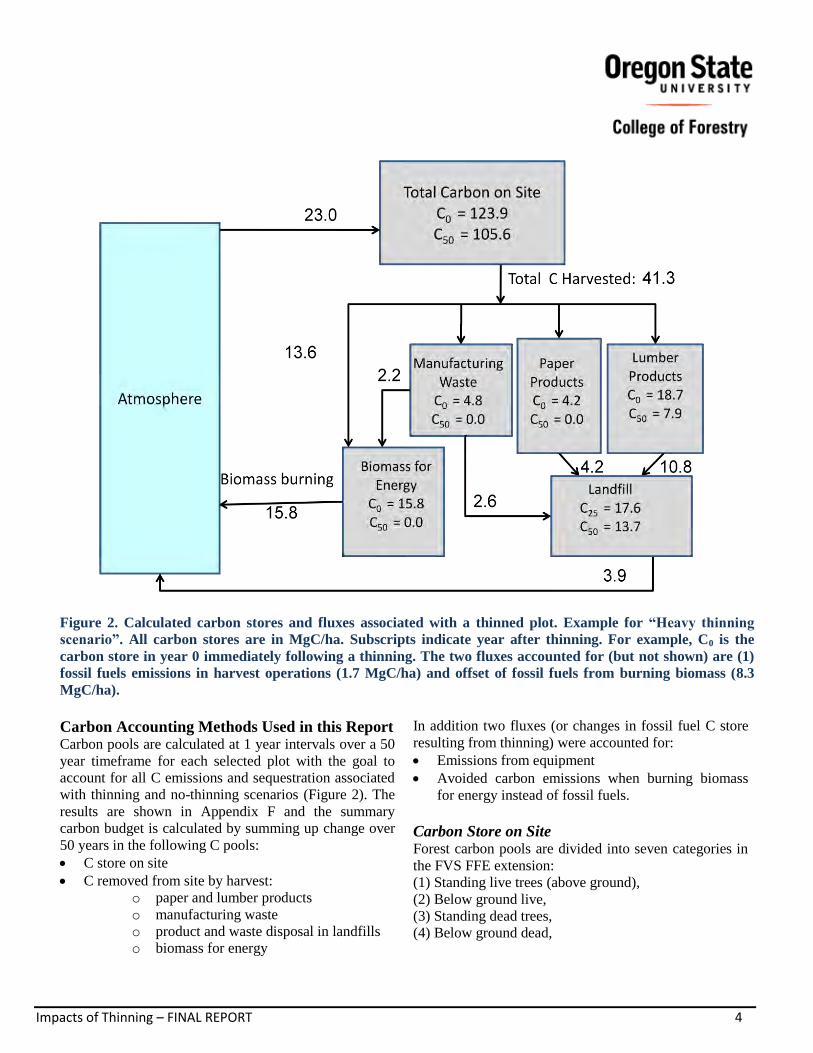
Figure 2 shows an example of carbon stores and
associated carbon fluxes used in calculations for this
report.
The stores are calculated as follows:
Total Carbon on Site – Carbon on site in any
given year.
Biomass for Energy – Carbon processed
(burned) for biomass energy in the year of
harvest. Combination of slash/small trees
(primary source) and residues from the
lumber/paper manufacturing process (secondary
source).
Lumber Products - Carbon store transferred to
lumber products from harvest and manufacturing
process.
Paper Products - Carbon store allocated to paper
products from harvest and manufacturing
process.
Paper/Lumber Residue – Carbon store
transferred to paper/lumber process, but not
converted to paper or lumber products. Some of
this store is allocated to biomass for energy, and
the remaining portion is assumed disposed in a
landfill (1% decay rate assumed – decay rate
used in other models: e.g., Hennigar et al. 2008).
Landfill – Carbon store to where paper and
lumber products are assumed transferred
following use. The landfill decay rate is assumed
to be 1%.
Some other carbon fluxes are not specifically
quantified in this report (e.g., impact of thinning on
soil carbon, fossil fuel emissions associated with
energy needs of product manufacturing, effects of
substitution of wood products for more energy-
intensive materials). Accounting for these additional
C fluxes is a complicated process and is beyond the
scope of this report. However, these factors
collectively would not be expected to change the
overall conclusions of the study.
Impacts of Thinning – FINAL REPORT 4
Figure 2. Calculated carbon stores and fluxes associated with a thinned plot. Example for “Heavy thinning
scenario”. All carbon stores are in MgC/ha. Subscripts indicate year after thinning. For example, C0 is the
carbon store in year 0 immediately following a thinning. The two fluxes accounted for (but not shown) are (1)
fossil fuels emissions in harvest operations (1.7 MgC/ha) and offset of fossil fuels from burning biomass (8.3
MgC/ha).
Carbon Accounting Methods Used in this Report Carbon pools are calculated at 1 year intervals over a 50
year timeframe for each selected plot with the goal to
account for all C emissions and sequestration associated
with thinning and no-thinning scenarios (Figure 2). The
results are shown in Appendix F and the summary
carbon budget is calculated by summing up change over
50 years in the following C pools:
C store on site
C removed from site by harvest:
o paper and lumber products
o manufacturing waste
o product and waste disposal in landfills
o biomass for energy
In addition two fluxes (or changes in fossil fuel C store
resulting from thinning) were accounted for:
Emissions from equipment
Avoided carbon emissions when burning biomass
for energy instead of fossil fuels.
Carbon Store on Site Forest carbon pools are divided into seven categories in
the FVS FFE extension:
(1) Standing live trees (above ground),
(2) Below ground live,
(3) Standing dead trees,
(4) Below ground dead,
Impacts of Thinning – FINAL REPORT 5
(5) Forest floor,
(6) Downed dead wood, and
(7) Shrubs and herbs.
The FVS-FFE extension simulates periodic carbon
estimates for each of the seven categories. The FVS-FFE
biomass estimates (and subsequent carbon estimates) do
not include stem bark biomass or stump biomass. Both
components have been manually added (using allometric
equations) for each tree. Additional details of the model
(including allometric equations) are included in
Appendix E.
The FVS-FFE model simulations for each thinning
prescription projects the following transfers of carbon:
C in roots of harvested trees is added to below
ground dead store.
C from slash, logging residue, and whole trees
≤3” DBH left on site following a thinning
scenario is added to downed dead wood.
Default regional decay rates with the FVS-FFE
model are used for slash/duff/litter.
C removed from the site is reported as “Carbon
removed”.
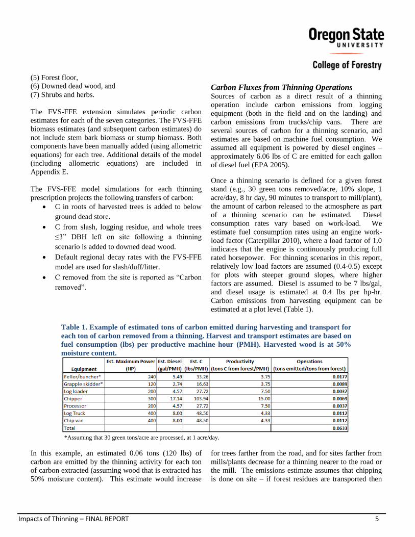
Carbon Fluxes from Thinning Operations Sources of carbon as a direct result of a thinning
operation include carbon emissions from logging
equipment (both in the field and on the landing) and
carbon emissions from trucks/chip vans. There are
several sources of carbon for a thinning scenario, and
estimates are based on machine fuel consumption. We
assumed all equipment is powered by diesel engines –
approximately 6.06 lbs of C are emitted for each gallon
of diesel fuel (EPA 2005).
Once a thinning scenario is defined for a given forest
stand (e.g., 30 green tons removed/acre, 10% slope, 1
acre/day, 8 hr day, 90 minutes to transport to mill/plant),
the amount of carbon released to the atmosphere as part
of a thinning scenario can be estimated. Diesel
consumption rates vary based on work-load. We
estimate fuel consumption rates using an engine work-
load factor (Caterpillar 2010), where a load factor of 1.0
indicates that the engine is continuously producing full
rated horsepower. For thinning scenarios in this report,
relatively low load factors are assumed (0.4-0.5) except
for plots with steeper ground slopes, where higher
factors are assumed. Diesel is assumed to be 7 lbs/gal,
and diesel usage is estimated at 0.4 lbs per hp-hr.
Carbon emissions from harvesting equipment can be
estimated at a plot level (Table 1).
Table 1. Example of estimated tons of carbon emitted during harvesting and transport for
each ton of carbon removed from a thinning. Harvest and transport estimates are based on
fuel consumption (lbs) per productive machine hour (PMH). Harvested wood is at 50%
moisture content.
*Assuming that 30 green tons/acre are processed, at 1 acre/day.
In this example, an estimated 0.06 tons (120 lbs) of
carbon are emitted by the thinning activity for each ton
of carbon extracted (assuming wood that is extracted has
50% moisture content). This estimate would increase
for trees farther from the road, and for sites farther from
mills/plants decrease for a thinning nearer to the road or
the mill. The emissions estimate assumes that chipping
is done on site – if forest residues are transported then

Impacts of Thinning – FINAL REPORT 6
chipped with an electric-powered chipper (more
efficient), overall carbon emissions would likely
decrease depending on load density of the transported
unchipped residues to the chipping location.
Carbon in harvested material Carbon removed from each plot by thinning was
estimated with FVS. The allocation of removed biomass
into forest products depends on many factors, including
regional market supply/demand, proximity of processing
facilities, wood product quality/species, log sizes, and
mill efficiencies. Several assumptions are made in order
to estimate final wood products.
In the model, trees are separated into 3 categories: (1)
smallest trees (<3” diameter over bark at breast height),
(2) small trees (>3” and < 6” diameter over bark at
breast height) and (2) larger trees (≥ 6” diameter over
bark at breast height). Smallest trees are trampled and
left in the field. Small trees have only one product use
(biomass for energy), but the end products for larger
trees are more diverse. Since most of the trees removed
in thinning are relatively small, it is assumed that all logs
greater than 6” DBH are transported to a sawmill and
then sawn into dimensional lumber, with residues used
for paper and energy or disposed of in a landfill.
Wood products are separated as follows:
Hog fuel (“dirty” chips): All smaller trees (< 6”
DBH) and the branches/tops for larger trees that
are transported to the landing are fed into a
chipper and processed into chips.
Primary sawmill products: Include dimensional
lumber.
Mill residues: Include “leftover” portions not
used in the primary product, such as bark,
sawdust, planer shavings, and chips.
o Bark – may be used for “beauty” bark, energy.
o Sawdust – may be used for paper, particle board.
o “Clean” chips – may be used for paper, particle
board.
Estimates of sawmill residues and final products are
available for Oregon (Brandt et al. 2006). The resulting
estimates of sawmill outputs are based on a statewide
average recovery factor of 2.07, which varies due to mill
efficiency, log size, and scaling. The carbon allocations
from mill gate to final product are used to estimate the
carbon transferred to various wood products (Figure 3).
We assume that lumber and paper products are separated
as 62% toward lumber and 27% toward paper.
.

Impacts of Thinning – FINAL REPORT 7
Figure 3. Estimated sawmill residues and final products (by weight), based on Brandt et al. 2006.
Manufacturing waste includes “Fuel”, “Other” and
“Unutilized” from Figure 3 as well as carbon from the
paper manufacturing process that is assumed not stored
within paper. The “Fuel” portion is assumed used toward
biomass for energy, and the remaining manufacturing
waste is assumed transferred to landfill (with a 1%
annual decay rate).
Carbon in wood products The amount of carbon retained in wood products over
time is estimated with an exponential function with set
half-lives for each wood product. The method used in
this report to estimate transferred carbon over time is
similar to the “simple decay” method (Ford-Robertson
2003).
where
There is a wide range of half-lives for wood products -
Table 2 shows some examples (Skog and Nicholson
1998). This report takes a simple approach - paper
products are assumed to have a half-life of 1 year, timber
products a half-life of 40 years, and biomass for energy
is assumed to be burned and emitted to the atmosphere
within a year.
Table 2. Harvested wood product estimated half-
life of carbon (years) for different end uses (Skog
and Nicholson 1998).
Carbon in landfill We assume that carbon that is not retained in wood
products (both paper and lumber) is transferred to
landfill. We make simplified calculations for this pool to

Impacts of Thinning – FINAL REPORT 8
estimate the amount at the end of 50-year projection
period (while all other pools are estimated on an annual
basis (Appendix F). The decomposition rate is 1% per
year and the time interval is 25 years (half of 50-year
projection period)
Carbon in slash harvested and utilized as source
for energy In the model for this study, all stems <3” DBH are
“trampled” (using an FVS keyword) and left on site.
This keyword affects crowning and torching index
estimates; trampled stems contribute to the downed dead
wood carbon pool. The amount of slash from larger
trees (>3” DBH) removed from the forest in a
mechanized logging operation varies widely. Removal
rate estimates of slash from cut-to-length mechanized
logging range from 50-75% (Mellström and Thörlind
1981; Sondell 1984).
It is assumed that the removal rate of slash is 80%, using
a whole-tree logging system for this study. We assume
that the slash removed from site is transported and
burned as biomass fuel, instead of piled and burned on
site. Transportation costs are included in the model.
The 20% of slash left on-site is included as downed-dead
wood, and decays over time using default FVS regional
decay rates.
In FVS, the torching and crowning indices are impacted
by increased fuel loading from slash but the effects are
seen only in the short term (less than 5 years) as the
slash decays. The effect of slash removal on soil
nutrients is an important site dependent factor that
should be considered (e.g. Page-Dumroese et al. 2010),
but an analysis is not included in this report.
Avoided carbon emissions - comparison of carbon
emissions between biomass and other energy
sources Both heat and electricity can be extracted from biomass.
The biomass input requirement per MW-hour for a
stand-alone biomass electric power generation plant
depends on biomass moisture content. The relationship
between input biomass and output electric power can be
found, assuming that 33% of energy output from the
boiler can be utilized for electric power (Table 3). The
dry tons of biomass required per MW-hour are a
function of biomass moisture content.
Table 3. Estimated forest biomass requirements as a function of wood moisture content.
Given the assumptions from Table 3, the carbon
emissions from biomass-produced energy from a stand-
alone unit can be estimated and compared to emissions
from alternative sources of energy (USDOE 2010)
(Table 4). The efficiency of a biomass plant depends on
moisture content – the analysis in Table 4 assumes 45%
moisture content for forest residues. Table 4 compares
carbon emissions between energy source alternatives for
biomass combined heat and power (CHP) units,
assuming 33% electrical conversion from the boiler.
Biomass fuel produces more CO2 per MW-hour
compared to other fossil fuel sources when used as a
stand-alone source for power. The difference between
biomass and fossil fuel is closer if electric power is not
generated, and instead 80% of the energy from the boiler
is used for heating. When comparing CO2 output
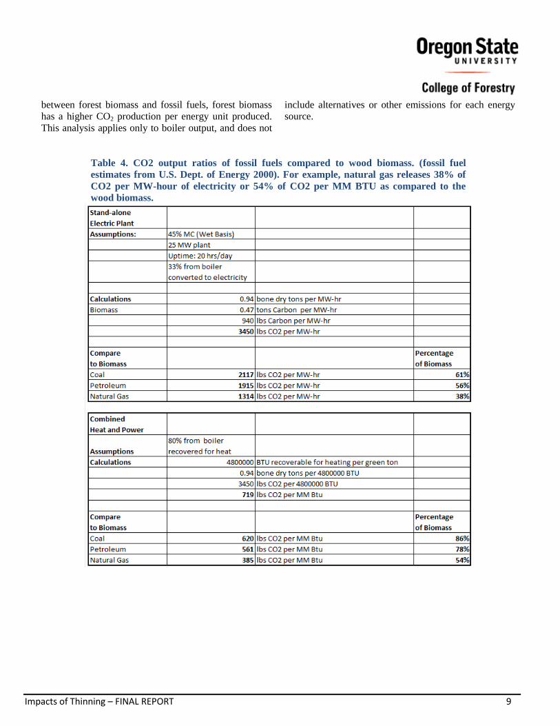
Impacts of Thinning – FINAL REPORT 9
between forest biomass and fossil fuels, forest biomass
has a higher CO2 production per energy unit produced.
This analysis applies only to boiler output, and does not
include alternatives or other emissions for each energy
source.
Table 4. CO2 output ratios of fossil fuels compared to wood biomass. (fossil fuel
estimates from U.S. Dept. of Energy 2000). For example, natural gas releases 38% of
CO2 per MW-hour of electricity or 54% of CO2 per MM BTU as compared to the
wood biomass.
Impacts of Thinning – FINAL REPORT 10
Carbon emissions for Energy Alternative There are several types of coal that are utilized for
electric power in the US, and can be classified by its
density of carbon. The CO2 output per pound of coal is
lower for ranks of coal with a lower percentage of
carbon, but the energy output per pound of coal is
smaller as well. Historically, not just carbon emissions
are considered when comparing different types of coal –
for instance, sulfur compounds are lower for sub-
bituminous coal. Coal plants find it cheaper to use coal
with lower sulfur content instead of scrubbing coal with
higher sulfur content. In the example, sub-bituminous
coal outputs are compared to biomass as a substitute
source of electric power. Production and transportation
emissions are relatively low, estimated as less than 2%
of potential energy produced for coal (Spath et al. 1999).
Life of Wood Products – Other Considerations At least three factors (not directly dealt with in this
report) make wood product life cycle assessments
difficult (Profft et al. 2009):
Wood products may be replaced by new products
before the physical end-of-use period, for a variety
of reasons.
Some long-lived products (e.g. laminated beams)
have largely unknown life spans.
Some wood waste is disposed of in landfills, and
burned wood waste may or may not be used toward
energy production.
Regional demands and mill locations may lead to
significantly different allocations to different wood
products. This could affect the allocation between long-
term and short-term wood products, particularly when
choosing between particleboard/medium density
fiberboard (MDF) (longer lifespan) vs. pulp/paper
products (shorter lifespan). Another effect will be the
final disposal of wood products. Products would release
carbon more quickly if they were burned for energy or
other purposes, as opposed to slower release of carbon
for wood products that are disposed of in a landfill
(Micales and Skog 1997).
Other Carbon Fluxes
Some of the carbon stores and fluxes within a forest as a
result of a thinning are recognized, but not quantified.
For example, a mechanical thinning will disturb the
forest soil (rutting and compaction), and increased
disturbance likely increases carbon flux from the soil.
However, the net effect on carbon pools within the soil
and soil respiration into the atmosphere, while
potentially relatively large, is difficult to measure (Ryu
et al. 2009), even though some estimates of carbon soil
losses have been estimated in agricultural processes
(e.g., Smith et al. 2010). As a result of the difficulty in
measuring soil carbon stores and fluxes (and no
estimates through FVS) it is not included in the model.
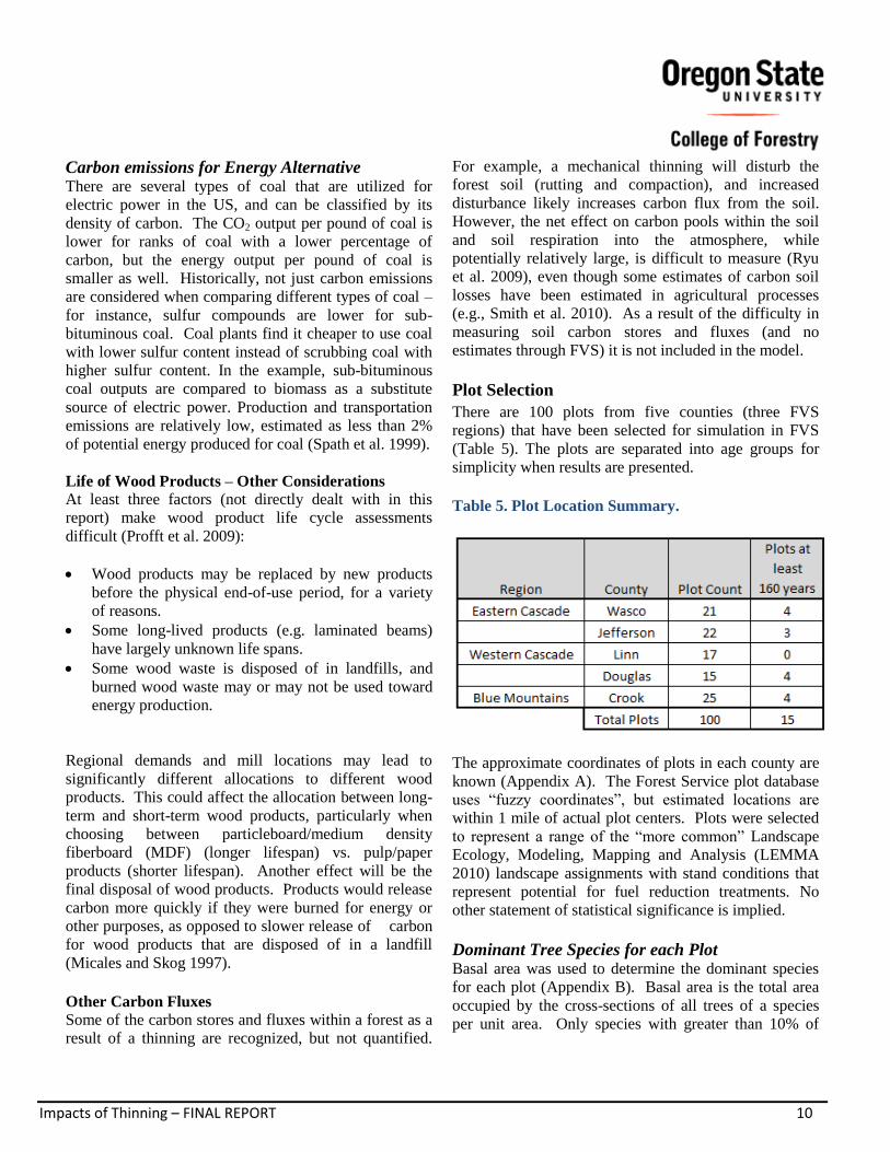
Plot Selection
There are 100 plots from five counties (three FVS
regions) that have been selected for simulation in FVS
(Table 5). The plots are separated into age groups for
simplicity when results are presented.
Table 5. Plot Location Summary.
The approximate coordinates of plots in each county are
known (Appendix A). The Forest Service plot database
uses “fuzzy coordinates”, but estimated locations are
within 1 mile of actual plot centers. Plots were selected
to represent a range of the “more common” Landscape
Ecology, Modeling, Mapping and Analysis (LEMMA
2010) landscape assignments with stand conditions that
represent potential for fuel reduction treatments. No
other statement of statistical significance is implied.
Dominant Tree Species for each Plot Basal area was used to determine the dominant species
for each plot (Appendix B). Basal area is the total area
occupied by the cross-sections of all trees of a species
per unit area. Only species with greater than 10% of

Impacts of Thinning – FINAL REPORT 11
total basal area are included for each plot in the tables
attached in Appendix B, so the cumulative percentage of
species for each plot does not always add up to 100% in
the tables. In the analysis, all trees are included in the
growth model. For most plots, the primary species are
Douglas-fir and ponderosa pine. Several other species
were commonly found in these plots, including white fir,
incense-cedar, and western hemlock.
Plot Understory Vegetation Plots that were measured from CVS had vegetation
codes (Hall 1998) that were input into FVS. Understory
vegetation is divided into four classes:
Forbs
Grasses
Shrubs
Trees
Vegetation species are reported by the number of plots
in which they occur (Appendix C). Understory species
were used in estimating the vegetation type when not
directly reported in the FIA database, but are considered
too bulky for this report. The tables use the following
definitions:
Species listed under “trees” refer to trees that are
currently growing at the same height as other
understory vegetation (shrubs, forbs, grasses).
This does not necessarily indicate the species of
the dominant trees within a plot.
Some of the species are ambiguous – for
example, “snowberry” is listed separately from
“common snowberry” and “creeping
snowberry”. The plant definitions for this study
are only as precise as the definitions that are
available from the source database.
Only the most common plants were included – if
a plant was counted in fewer than 3 plots, it is
not included in the summary (but is available).
Table C5 summarizes the number of different plants/
plant groups within each vegetation class that were
counted for each plot in four counties.
Carbon Pool Estimates for Plots Prior to
Treatment The Fuels and Fire Extension (FFE) to the Forest
Vegetation Simulator (FVS) has integrated reports that
estimate forest carbon pools as forest stand growth is
simulated. Carbon pool estimates are separated into
seven categories:
Standing live trees
Belowground live
Standing dead trees
Belowground dead
Downed dead wood (including coarse woody debris)
Forest floor (including duff)
Shrubs and herbs
In this analysis, each plot is grown in FVS for 50 years –
both the initial carbon pool as well as carbon growth
rates are examined and compared to forest volume
growth rates to determine site productivity. FVS uses
region-specific variants that adjust growth conditions
based on regional differences. The Eastern Cascade,
Western Cascade, and Blue Mountains variants are used
in this study. The plots from each county use the variant
recommended by FVS for that county. All plots are
simulated and analyzed separately, but only a few of the
plots are shown in this report. Plots are chosen from a
range of initial conditions. A more detailed explanation
of FVS calculations is in Appendix E.
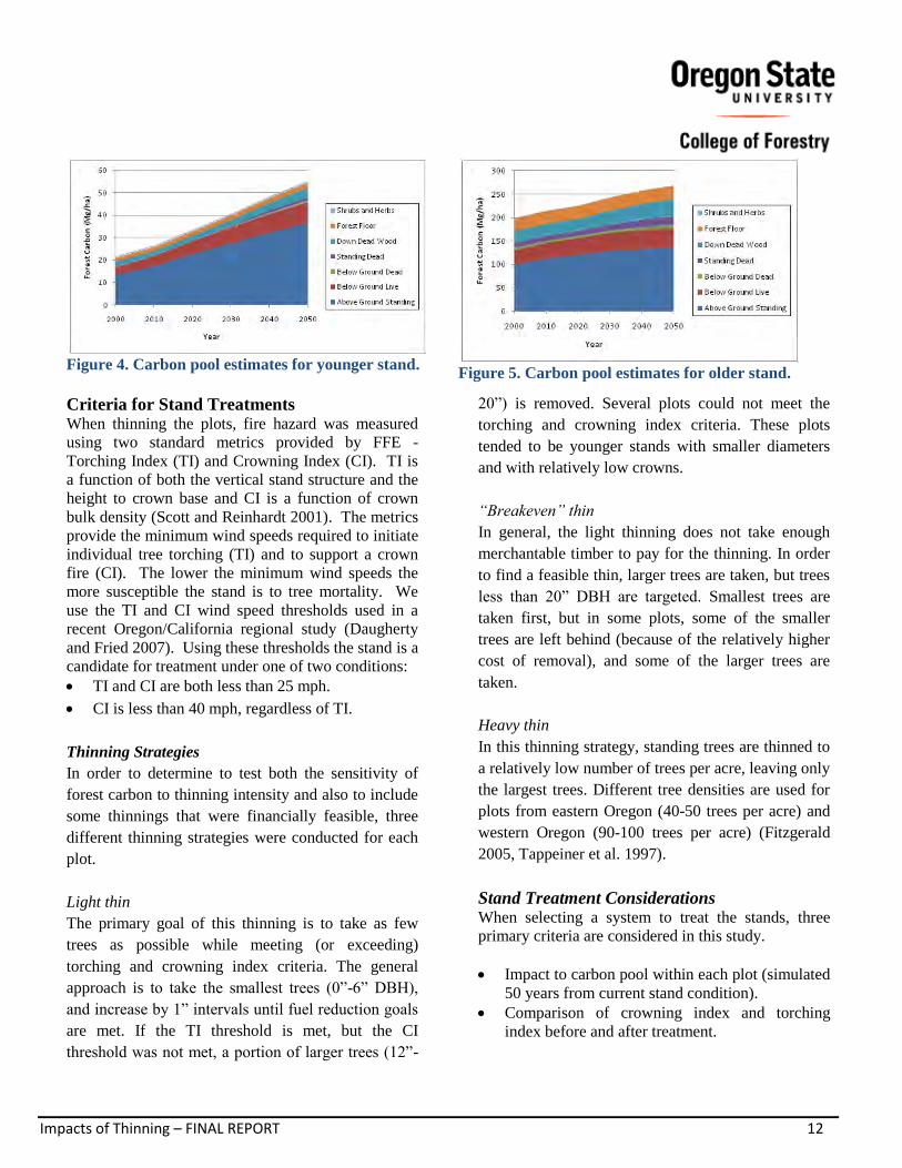
Figure 4 shows carbon estimates for a relatively young
stand and Figure 5 for a relatively older stand, assuming
no thinning. Note the difference in carbon scales – there
is a much lower amount of carbon in the younger stand,
but the percentage increase from initial carbon for the
younger stand is much higher over the 50-year time
frame.
Impacts of Thinning – FINAL REPORT 12
Figure 4. Carbon pool estimates for younger stand.
Figure 5. Carbon pool estimates for older stand.
Criteria for Stand Treatments When thinning the plots, fire hazard was measured
using two standard metrics provided by FFE -
Torching Index (TI) and Crowning Index (CI). TI is
a function of both the vertical stand structure and the
height to crown base and CI is a function of crown
bulk density (Scott and Reinhardt 2001). The metrics
provide the minimum wind speeds required to initiate
individual tree torching (TI) and to support a crown
fire (CI). The lower the minimum wind speeds the
more susceptible the stand is to tree mortality. We
use the TI and CI wind speed thresholds used in a
recent Oregon/California regional study (Daugherty
and Fried 2007). Using these thresholds the stand is a
candidate for treatment under one of two conditions:
TI and CI are both less than 25 mph.
CI is less than 40 mph, regardless of TI.
Thinning Strategies
In order to determine to test both the sensitivity of
forest carbon to thinning intensity and also to include
some thinnings that were financially feasible, three
different thinning strategies were conducted for each
plot.
Light thin
The primary goal of this thinning is to take as few
trees as possible while meeting (or exceeding)
torching and crowning index criteria. The general
approach is to take the smallest trees (0”-6” DBH),
and increase by 1” intervals until fuel reduction goals
are met. If the TI threshold is met, but the CI
threshold was not met, a portion of larger trees (12”-
20”) is removed. Several plots could not meet the
torching and crowning index criteria. These plots
tended to be younger stands with smaller diameters
and with relatively low crowns.
“Breakeven” thin
In general, the light thinning does not take enough
merchantable timber to pay for the thinning. In order
to find a feasible thin, larger trees are taken, but trees
less than 20” DBH are targeted. Smallest trees are
taken first, but in some plots, some of the smaller
trees are left behind (because of the relatively higher
cost of removal), and some of the larger trees are
taken.
Heavy thin
In this thinning strategy, standing trees are thinned to
a relatively low number of trees per acre, leaving only
the largest trees. Different tree densities are used for
plots from eastern Oregon (40-50 trees per acre) and
western Oregon (90-100 trees per acre) (Fitzgerald
2005, Tappeiner et al. 1997).
Stand Treatment Considerations When selecting a system to treat the stands, three
primary criteria are considered in this study.
Impact to carbon pool within each plot (simulated
50 years from current stand condition).
Comparison of crowning index and torching
index before and after treatment.
Impacts of Thinning – FINAL REPORT 13
Economics of the treatment (treatment must pay
for itself for the breakeven thinning scenario).
Other criteria that are important to consider, but
beyond the scope of this study, include
Laws/regulations and public acceptance of
potential treatments, particularly on public lands.
Safety standards and certifications of contractors
hired for potential thinning.
A financial analysis was conducted using the Fuel
Reduction Cost Simulator (FRCS-West 2010) and
LogCost10.2 (2010), while the FVS FFE extension is
used to estimate the Torching Index (TI) and
Crowning Index (CI), both of which measure stand
conditions and hazards that may contribute to a
catastrophic fire. The effectiveness of fuel treatment
was assessed based on TI and CI estimates before and
after thinning. A detailed analysis of TI and CI at a
group level is in Figure F1 and F2.
A financial break-even point (where revenues and
cost are equal) depends upon a host of factors, some
of which are known, and some of which are
estimated. There are many potential fuel treatments
available within FRCS, including ground-based
operations and cable-based operations. In general, the
lowest cost systems are ground-based. Ground-based
thinning operations can be separated into whole-tree
and cut-to-length operations, both which have
advantages and disadvantages. One harvesting
system is used for plots on more gentle terrain (slopes
≤ 30%), and a slightly different system is used for
plots with steeper terrain (slopes >30%).
For more gentle slopes, the following whole-tree
system is used:
Drive-to-tree feller/buncher
Grapple skidder
Processing/chipping/loading at the landing
Truck and trailer transport to nearest mill/plant.
For steeper slopes, the drive-to tree feller/buncher is
replaced with a swing-boom feller/buncher, which is
more stable on steeper slopes, but is limited to the
length of the boom and may lead to less flexibility in
tree removal. For longer skidding distances, the cut-
to-length system (CTL) becomes less expensive than
whole-tree skidding due to the higher load carrying
capability of forwarders. CTL systems can also have
lower mobilization costs, important in small, low
volume treatment units, because fewer pieces of
equipment are transported between harvest units.
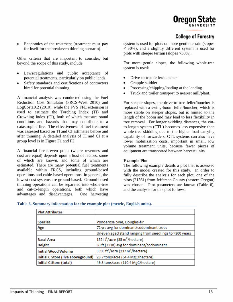
Example Plot
The following example details a plot that is assessed
with the model created for this study. In order to
fully describe the analysis for each plot, one of the
plots (21561) from Jefferson County (eastern Oregon)
was chosen. Plot parameters are known (Table 6),
and the analysis for this plot follows.
Table 6. Summary information for the example plot (metric, English units).
Impacts of Thinning – FINAL REPORT 14
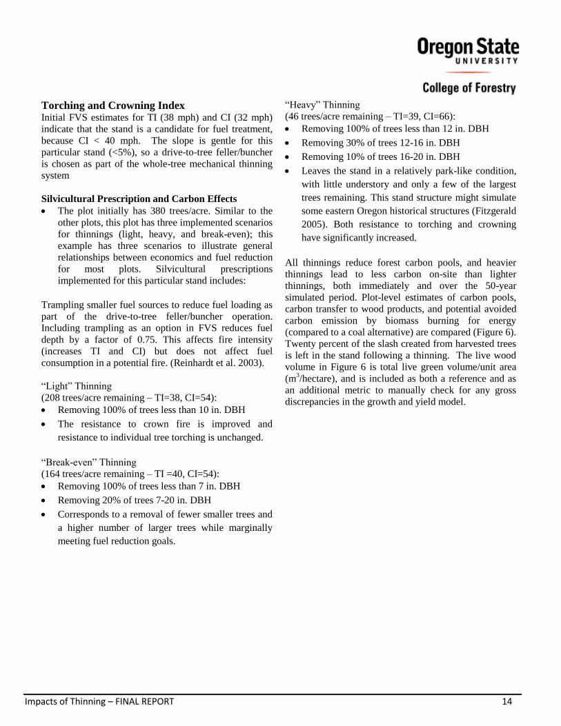
Torching and Crowning Index Initial FVS estimates for TI (38 mph) and CI (32 mph)
indicate that the stand is a candidate for fuel treatment,
because CI < 40 mph. The slope is gentle for this
particular stand (<5%), so a drive-to-tree feller/buncher
is chosen as part of the whole-tree mechanical thinning
system
Silvicultural Prescription and Carbon Effects
The plot initially has 380 trees/acre. Similar to the
other plots, this plot has three implemented scenarios
for thinnings (light, heavy, and break-even); this
example has three scenarios to illustrate general
relationships between economics and fuel reduction
for most plots. Silvicultural prescriptions
implemented for this particular stand includes:
Trampling smaller fuel sources to reduce fuel loading as
part of the drive-to-tree feller/buncher operation.
Including trampling as an option in FVS reduces fuel
depth by a factor of 0.75. This affects fire intensity
(increases TI and CI) but does not affect fuel
consumption in a potential fire. (Reinhardt et al. 2003).
“Light” Thinning
(208 trees/acre remaining – TI=38, CI=54):
Removing 100% of trees less than 10 in. DBH
The resistance to crown fire is improved and
resistance to individual tree torching is unchanged.
“Break-even” Thinning
(164 trees/acre remaining – TI =40, CI=54):
Removing 100% of trees less than 7 in. DBH
Removing 20% of trees 7-20 in. DBH
Corresponds to a removal of fewer smaller trees and
a higher number of larger trees while marginally
meeting fuel reduction goals.
“Heavy” Thinning
(46 trees/acre remaining – TI=39, CI=66):
Removing 100% of trees less than 12 in. DBH
Removing 30% of trees 12-16 in. DBH
Removing 10% of trees 16-20 in. DBH
Leaves the stand in a relatively park-like condition,
with little understory and only a few of the largest
trees remaining. This stand structure might simulate
some eastern Oregon historical structures (Fitzgerald
2005). Both resistance to torching and crowning
have significantly increased.
All thinnings reduce forest carbon pools, and heavier
thinnings lead to less carbon on-site than lighter
thinnings, both immediately and over the 50-year
simulated period. Plot-level estimates of carbon pools,
carbon transfer to wood products, and potential avoided
carbon emission by biomass burning for energy
(compared to a coal alternative) are compared (Figure 6).
Twenty percent of the slash created from harvested trees
is left in the stand following a thinning. The live wood
volume in Figure 6 is total live green volume/unit area
(m3/hectare), and is included as both a reference and as
an additional metric to manually check for any gross
discrepancies in the growth and yield model.

Impacts of Thinning – FINAL REPORT 15
Figure 6. Simulation of carbon pools for the forest stand – No Thin (top), Light Thin (middle)
and Heavy Thin (bottom).
All carbon components reference the left axis. Only standing green tree volume (Volume)
references the right axis.
Impacts of Thinning – FINAL REPORT 16
Harvesting System The harvesting system for this stand includes five major
pieces of equipment and two types of transportation
vehicles:
Drive-to-tree feller/buncher – Mechanically falls
each tree and lays trees into groups (bunches) for
efficient handling.
Grapple skidder – Grabs whole tree bunches and
drags trees to a roadside landing.
Processor – Located at the roadside landing.
Delimbs and bucks trees into merchantable lengths.
Chipper – Located at the roadside landing. Chips
small whole trees (< 6” DBH) and tops and branches
from larger trees directly into a chip van.
Loader – Located at the roadside landing.
Maneuvers small whole trees and residues into the
chipper and logs into log trucks.
Truck with Chip Van – Transports chips from
landing to destination. Capacity for vans in this
example is 110 cubic yards.
Truck with Log Trailer – Transports logs from
landing to mill.
This is a thinning system that removes whole trees to the
landing. There is a potential for residual stand damage
that must be considered in both harvest planning and
operations.
A Cut-to-Length (CTL) system could be used at a
comparatively lower cost for thinning at longer skidding
distances when compared to a whole-tree system
(Kellogg et al. 2010), but a CTL system was not
included in the final economic analysis, since average
skidding distance in this report is assumed to be 500 feet
(also assumed by Dempster el al. 2008).
Costs Costs are separated into four components:
Planning/administration costs – includes timber sale
preparation and administration. Sales preparation and
administration estimates for nonfederal (Nall 2010,
Sessions et al. 2000) and national forest land
(TSPIRS 2001, adjusted for inflation) are estimated in
Table 7. The federal land administrative costs are not
included in the “breakeven” analysis, and
administrative costs vary widely from sale to sale,
according to federal requirements, including
compliance with the National Environmental Policy
Act (NEPA) and other federal laws (e.g., USFS
2010). In general, federal land sales preparation and
administration costs are higher compared to private
land. The estimate used in the example is a general
example only, and should not be used to estimate
actual costs.
Setup costs – includes one-time move-in cost to an
area, moving costs from landing to landing, sales
preparation cost, and road maintenance costs (Table
8).
Cost from field to truck, including felling/bunching,
skidding, chipping, processing, and loading (Table
9).
Cost to transport each wood product (Table 10).
The planning/administration costs are shown, but are not
included in the final analysis.

Impacts of Thinning – FINAL REPORT 17
Table 7. Sales preparation and administration costs associated with the three thinning scenarios.
Table 8. Estimated equipment setup costs for the three thinning scenarios.
Table 9. Estimated costs from field to truck for the three thinning scenarios.
Table 10. Estimated truck transport cost for the three thinning scenarios.
Wood Products The volume and mix of wood products derived from the
thinning is critical when calculating total revenue from
the stand. The mix of trees removed from the plot is
separated by diameter class (Table 11). FVS simulated
the total volume (ft3) per plot and merchantable volume
(Mbf) in order to estimate timber value. A 16 ft scaling
rule (Scribner) was used for plots in eastern Oregon, and

Impacts of Thinning – FINAL REPORT 18
the midrange diameter was used to estimate the Mbf:cf
ratio for each diameter class (e.g., 7” was used for 6”- 8” sawtimber) which was found with a conversion chart
(Mann and Lysons 1972 – Fig 4).
Table 11. Allocation of thinned trees into wood products.
Sawlog prices are estimated using the Oregon
Department of Forestry Log Price Information (Oregon
Dept. of Forestry 2010). The biomass market returns
significantly lower prices than the pulp market, but it is
assumed that the biomass chip quality does not meet
pulp chip standards (Table 12).
Table 12. Estimated delivered harvested wood
product prices.
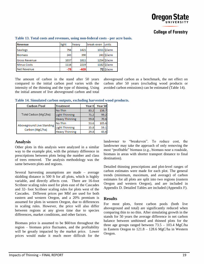
Overall Cost/Revenue Analysis For this particular scenario with the given assumptions,
there is a net profit of $72/acre for the “breakeven thin”
scenario on non-federal lands (Table 13). Both the
“light” and “heavy” thin result in treatment costs
exceeding revenues given the initial assumptions. These
three different thinning scenarios demonstrate that
increasing gross revenue or total volume does not
necessarily improve net revenue, and depending on
original stand structure, may significantly increase
harvesting costs. In order for this thinning to not incur
financial losses on federal lands, a relatively high
proportion of high-value stems and a relatively low
proportion of low-value stems would need to be thinned.
Impacts of Thinning – FINAL REPORT 19
Table 13. Total costs and revenues, using non-federal costs - per acre basis.
The amount of carbon in the stand after 50 years
compared to the initial carbon pool varies with the
intensity of the thinning and the type of thinning. Using
the initial amount of live aboveground carbon and total
aboveground carbon as a benchmark, the net effect on
carbon after 50 years (excluding wood products or
avoided carbon emissions) can be estimated (Table 14).
Table 14. Simulated carbon outputs, excluding harvested wood products.
Analysis
Other plots in this analysis were analyzed in a similar
way to the example plot, with the primary difference in
prescriptions between plots being the number and class
of trees removed. The analysis methodology was the
same between plots and regions.
Several harvesting assumptions are made – average
skidding distance is 500 ft for all plots, which is highly
variable, and directly affects cost. There are 16-foot
Scribner scaling rules used for plots east of the Cascades
and 32- foot Scribner scaling rules for plots west of the
Cascades. Different prices per Mbf are used for both
eastern and western Oregon, and a 20% premium is
assumed for plots in western Oregon, due to differences
in scaling rules. However, the price will also differ
between regions at any given time due to species
differences, market conditions, and other factors.
Biomass price is assumed to be $60/ton throughout the
region – biomass price fluctuates, and the profitability
will be greatly impacted by the market price. Lower
prices would make it much more difficult for the
landowner to “breakeven”. To reduce cost, the
landowner may take the approach of only removing the
most “profitable” biomass (e.g., biomass near a roadside,
biomass in areas with shorter transport distance to final
destination).
Detailed thinning prescriptions and plot-level ranges of
carbon estimates were made for each plot. The general
trends (minimum, maximum, and average) of carbon
estimates for all plots are split into two regions (eastern
Oregon and western Oregon), and are included in
Appendix D. Detailed Tables are included (Appendix F).
Results For most plots, forest carbon pools (both live
aboveground and total) are significantly reduced when
comparing thin to no thin. After simulating growth in the
stands for 50 years the average difference in net carbon
balance between unthinned and thinned plots for the
three age groups ranged between 73.5 – 103.4 MgC/ha
in Eastern Oregon to 121.8 – 128.6 MgC/ha in Western
Oregon.
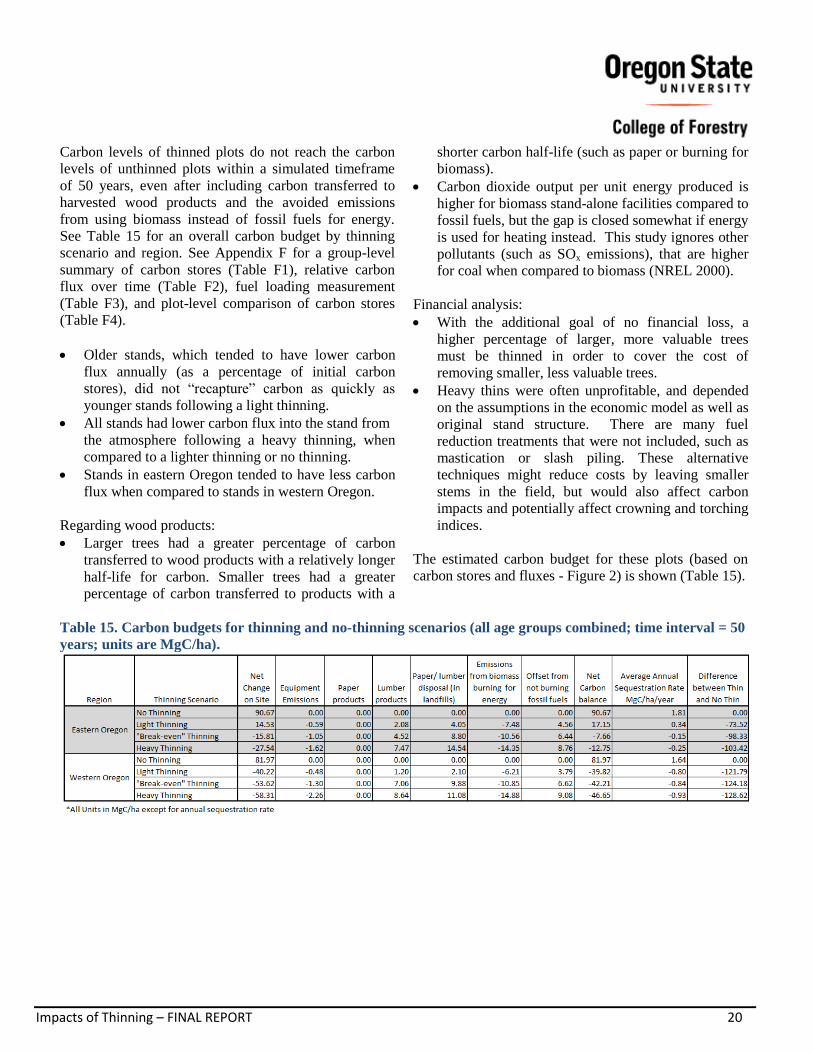
Impacts of Thinning – FINAL REPORT 20
Carbon levels of thinned plots do not reach the carbon
levels of unthinned plots within a simulated timeframe
of 50 years, even after including carbon transferred to
harvested wood products and the avoided emissions
from using biomass instead of fossil fuels for energy.
See Table 15 for an overall carbon budget by thinning
scenario and region. See Appendix F for a group-level
summary of carbon stores (Table F1), relative carbon
flux over time (Table F2), fuel loading measurement
(Table F3), and plot-level comparison of carbon stores
(Table F4).
Older stands, which tended to have lower carbon
flux annually (as a percentage of initial carbon
stores), did not “recapture” carbon as quickly as
younger stands following a light thinning.
All stands had lower carbon flux into the stand from
the atmosphere following a heavy thinning, when
compared to a lighter thinning or no thinning.
Stands in eastern Oregon tended to have less carbon
flux when compared to stands in western Oregon.
Regarding wood products:
Larger trees had a greater percentage of carbon
transferred to wood products with a relatively longer
half-life for carbon. Smaller trees had a greater
percentage of carbon transferred to products with a
shorter carbon half-life (such as paper or burning for
biomass).
Carbon dioxide output per unit energy produced is
higher for biomass stand-alone facilities compared to
fossil fuels, but the gap is closed somewhat if energy
is used for heating instead. This study ignores other
pollutants (such as SOx emissions), that are higher
for coal when compared to biomass (NREL 2000).
Financial analysis:
With the additional goal of no financial loss, a
higher percentage of larger, more valuable trees
must be thinned in order to cover the cost of
removing smaller, less valuable trees.
Heavy thins were often unprofitable, and depended
on the assumptions in the economic model as well as
original stand structure. There are many fuel
reduction treatments that were not included, such as
mastication or slash piling. These alternative
techniques might reduce costs by leaving smaller
stems in the field, but would also affect carbon
impacts and potentially affect crowning and torching
indices.
The estimated carbon budget for these plots (based on
carbon stores and fluxes - Figure 2) is shown (Table 15).
Table 15. Carbon budgets for thinning and no-thinning scenarios (all age groups combined; time interval = 50
years; units are MgC/ha).
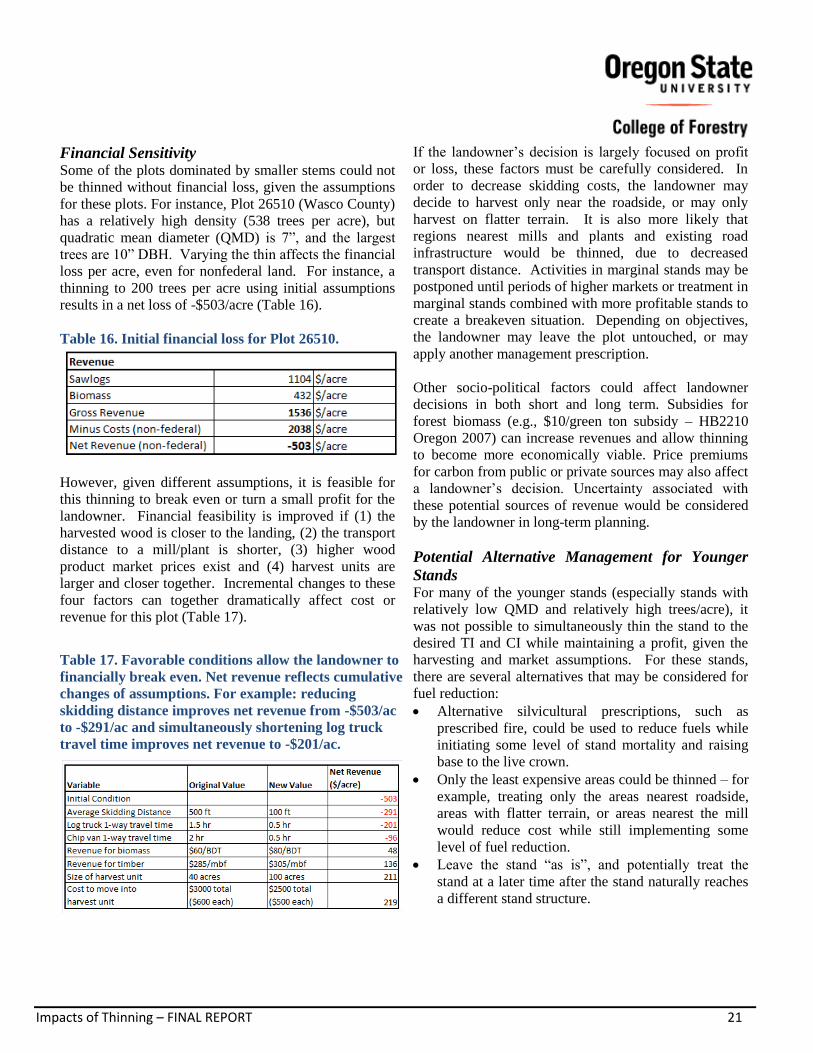
Impacts of Thinning – FINAL REPORT 21
Financial Sensitivity Some of the plots dominated by smaller stems could not
be thinned without financial loss, given the assumptions
for these plots. For instance, Plot 26510 (Wasco County)
has a relatively high density (538 trees per acre), but
quadratic mean diameter (QMD) is 7”, and the largest
trees are 10” DBH. Varying the thin affects the financial
loss per acre, even for nonfederal land. For instance, a
thinning to 200 trees per acre using initial assumptions
results in a net loss of -$503/acre (Table 16).
Table 16. Initial financial loss for Plot 26510.
However, given different assumptions, it is feasible for
this thinning to break even or turn a small profit for the
landowner. Financial feasibility is improved if (1) the
harvested wood is closer to the landing, (2) the transport
distance to a mill/plant is shorter, (3) higher wood
product market prices exist and (4) harvest units are
larger and closer together. Incremental changes to these
four factors can together dramatically affect cost or
revenue for this plot (Table 17).
Table 17. Favorable conditions allow the landowner to
financially break even. Net revenue reflects cumulative
changes of assumptions. For example: reducing
skidding distance improves net revenue from -$503/ac
to -$291/ac and simultaneously shortening log truck
travel time improves net revenue to -$201/ac.
If the landowner’s decision is largely focused on profit
or loss, these factors must be carefully considered. In
order to decrease skidding costs, the landowner may
decide to harvest only near the roadside, or may only
harvest on flatter terrain. It is also more likely that
regions nearest mills and plants and existing road
infrastructure would be thinned, due to decreased
transport distance. Activities in marginal stands may be
postponed until periods of higher markets or treatment in
marginal stands combined with more profitable stands to
create a breakeven situation. Depending on objectives,
the landowner may leave the plot untouched, or may
apply another management prescription.
Other socio-political factors could affect landowner
decisions in both short and long term. Subsidies for
forest biomass (e.g., $10/green ton subsidy – HB2210
Oregon 2007) can increase revenues and allow thinning
to become more economically viable. Price premiums
for carbon from public or private sources may also affect
a landowner’s decision. Uncertainty associated with
these potential sources of revenue would be considered
by the landowner in long-term planning.
Potential Alternative Management for Younger
Stands For many of the younger stands (especially stands with
relatively low QMD and relatively high trees/acre), it
was not possible to simultaneously thin the stand to the
desired TI and CI while maintaining a profit, given the
harvesting and market assumptions. For these stands,
there are several alternatives that may be considered for
fuel reduction:
Alternative silvicultural prescriptions, such as
prescribed fire, could be used to reduce fuels while
initiating some level of stand mortality and raising
base to the live crown.
Only the least expensive areas could be thinned – for
example, treating only the areas nearest roadside,
areas with flatter terrain, or areas nearest the mill
would reduce cost while still implementing some
level of fuel reduction.
Leave the stand “as is”, and potentially treat the
stand at a later time after the stand naturally reaches
a different stand structure.
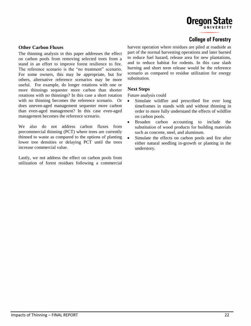
Impacts of Thinning – FINAL REPORT 22
Other Carbon Fluxes
The thinning analysis in this paper addresses the effect
on carbon pools from removing selected trees from a
stand in an effort to improve forest resilience to fire.
The reference scenario is the “no treatment” scenario.
For some owners, this may be appropriate, but for
others, alternative reference scenarios may be more
useful. For example, do longer rotations with one or
more thinnings sequester more carbon than shorter
rotations with no thinnings? In this case a short rotation
with no thinning becomes the reference scenario. Or
does uneven-aged management sequester more carbon
than even-aged management? In this case even-aged
management becomes the reference scenario.
We also do not address carbon fluxes from
precommercial thinning (PCT) where trees are currently
thinned to waste as compared to the options of planting
lower tree densities or delaying PCT until the trees
increase commercial value.
Lastly, we not address the effect on carbon pools from
utilization of forest residues following a commercial
harvest operation where residues are piled at roadside as
part of the normal harvesting operations and later burned
to reduce fuel hazard, release area for new plantations,
and to reduce habitat for rodents. In this case slash
burning and short term release would be the reference
scenario as compared to residue utilization for energy
substitution.
Next Steps
Future analysis could
Simulate wildfire and prescribed fire over long
timeframes in stands with and without thinning in
order to more fully understand the effects of wildfire
on carbon pools.
Broaden carbon accounting to include the
substitution of wood products for building materials
such as concrete, steel, and aluminum.
Simulate the effects on carbon pools and fire after
either natural seedling in-growth or planting in the
understory.
Impacts of Thinning – FINAL REPORT 23
Contact Information Joshua Clark, PhD
Postdoctoral Researcher
Forest Engineering, Resources and Management (FERM) Department
Oregon State University
Email: [email protected]
John Sessions, PhD
Professor
FERM Department
Oregon State University
http://ferm.forestry.oregonstate.edu/facstaff/sessions-julian
Email: [email protected]
Olga Krankina, PhD
Associate Professor
Forest Ecosystems and Society (FES) Department
Oregon State University
http://fes.forestry.oregonstate.edu/faculty/krankina-olga
Email: [email protected]
Thomas Maness, PhD
Professor and Department Head
FERM Department
Oregon State University
http://ferm.forestry.oregonstate.edu/facstaff/maness-thomas
Email: [email protected]
Impacts of Thinning – FINAL REPORT 24
References
Adams, D.M.; Latta, G.S. 2003. Private timber harvest
potential in Eastern Oregon. OSU Forest Research Lab.
Research Contribution 42. 46 p.
Bessie, W. C.; Johnson, E.A. 1995. The relative
importance of fuels and weather on fire behavior in
subalpine forests. Ecology. 76. pp. 747–762.
Börjesson, P.; Gustavsson, L. 2000. Greenhouse gas
balances in building construction: wood versus concrete
from life-cycle and forest land-use perspectives. Energy
Policy. 28. pp.575-588.
Böttcher, H. 2007. Dissertation. Modeling of Forestry
Options, their Impact on the Regional Carbon Balance
and Implications for a Future Climate Protocol.
Bouffier, L.A.; Gartner, B.L.; Domec, J. 2003. Wood
Density and Hydraulic Properties of Ponderosa Pine
from the Willamette Valley vs. the Cascade Mountains.
Wood and Fiber Science. 35(2). pp. 217-233.
Brandt, J.P.; Morgan, T.A.; Dillon, T.; Lettman, G.J.;
Keegan, C.E.; Azuma, D.L. 2006. Oregon’s forest
products industry and timber harvest, 2003. General
Technical Report PNW-GTR-681. Portland, OR: U.S.
Department of Agriculture, Forest Service, Pacific
Northwest Research Station. 53 p.
Brinker, R.W.; Kinard, J.; Rummer, B.; Lanford, B.
2002. Machine rates for selected forest harvesting
machines. Circular 296 (revised). Auburn University,
Auburn, AL. 32 p.
Caterpillar. 2010. Caterpillar performance handbook,
40th Ed., Caterpillar, Inc., Peoria, Ill.
Crookston, N.L. 1990. User’s Guide to the Event
Monitor: Part of Prognosis Model Version 6. General
Technical Report INT-GTR-275. Ogden, UT: U.S.
Department of Agriculture, Forest Service,
Intermountain Research Station. 21 p.
Crookston, N. L. 1997. Suppose: An Interface to the
Forest Vegetation Simulator. In: Teck, R.; Moeur, M.;
Adams, J. 1997. Proceeding: Forest vegetation
simulator conference. 1997 Feb. 3-7, Fort Collins, CO.
General Technical Report INT-GTR-373. Ogden, UT:
U.S. Department of Agriculture, Forest Service,
Intermountain Research Station.
Current Vegetation Survey (CVS). [Accessed 24 June
2010 from http://www.fs.fed.us/r6/survey/].
Dale, V.H.; Joyce, L.A.; McNulty, S.; Neilson, R.P.;
Ayres, M.P.; Irland, L.C.; Lugo, A.E.; Peterson, C.J.;
Simberloff, D.; Swanson, F.J.; Stocks, B.J; Wotton, M.
2001. Climate change and forest disturbances.
BioScience. 51(9). pp. 723-734.
Daugherty, P.J.; Fried, J.S. 2007. Jointly optimizing
selection of fuel treatments and siting of forest biomass-
based energy production facilities for landscape-scale
fire-hazard-reduction. Information Systems and
Operational Research. 45(1). pp. 353–372.
Dempster, P.; Gallo, N.; Hartsough, B.; Jenkins, B.;
Tittmann, P. 2008. Biomass Harvesting Equipment and
Conversion Technology Review. The California Biomass
Collaborative. 124 p.
Dushku, A.; Brown S.; Petrova, S.; Pearson, T.; Martin,
N.; Winsten, J.; Kadyszewski, J. (Winrock Int.). 2007.
Carbon Sequestration Through Changes in Land Use in
Oregon: Costs and Opportunities. California Energy
Commission, PIER Energy‐Related Environmental
Research Program. CEC‐500‐2007‐074. 100 p.
Environmental Protection Agency (EPA). 2005. Average
Carbon Dioxide Emissions Resulting from Gasoline and
Diesel Fuel. [Accessed 12 Sept. 2010 from
http://www.epa.gov/otaq/climate/420f05001.pdf].
Fiedler, C.E.; Arno, S.F.; Harrington, M.G. 1998.
Reintroducing fire in ponderosa pine-fir forests after a
century of fire exclusion. In: T.L. Pruden and L.A.
Brennan, Editors, Proceedings of the 20th Tall Timbers
Fire Ecology Conference, Tall Timbers Research
Station, Tallahassee, FL. pp. 245–249.

Impacts of Thinning – FINAL REPORT 25
Fight, R. D.; Hartsough, B.R.; Noordijk, P. 2006. Users
guide for FRCS: fuel reduction cost simulator software.
General Technical Report PNW-GTR-668. Portland,
OR: U.S. Department of Agriculture, Forest Service,
Pacific Northwest Research Station. 23 p. [Accessed 6
August 2010 from http://www.fs.fed.us/pnw/pubs/pnw_gtr668.pdf].
Finney, M.A., Seli, R.C.; McHugh, C.W.; Ager, A.A.;
Bahro, B.; Agee, J.K. 2006. Simulation of long-term
landscape-level fuel treatment effects on large wildfires.
In: Andrews, P.L., Butler, B.W. (Eds.) (Comps), Fuels
Management - How to Measure Success: Conference
Proceedings, March 28–30, Portland, OR, U.S.
Department of Agriculture, Forest Service, Rocky
Mountain Research Station Proceedings RMRS-P-41,
pp. 125–148.
Fitzgerald, S.A. 2005. Fire ecology of ponderosa pine
and the rebuilding of fire-resistant ponderosa pine
ecosystems. In: Ritchie, M.W., Maguire, D.A.,
Youngblood, A. (Technical Coordinators), Proceedings
of the Symposium on Ponderosa Pine: Issues, Trends,
and Management. General Technical Report PSW-GTR-
198. U.S. Department of Agriculture, Forest Service. pp.
197–225.
Ford-Robertson, J. 2003. Implications of harvested
wood products accounting. Analysis of issues raised by
Parties to the UNFCCC and development of a simple
decay approach. MAF Technical Paper No. 2003/5, 30 p.
Ministry of Agriculture and Forestry, Wellington, New
Zealand.
Forest Inventory and Analysis (FIA) database v4.0.
2010. Accessed 24 June 2010 from
http://199.128.173.17/fiadb4downloads/datamart.html].
Fuel Reduction Cost Simulator (FRCS) -West (Excel
spreadsheet). 2010. [Accessed 6 August 2010 from
http://www.fs.fed.us/pnw/data/frcs/frcs.shtml].
Forest Vegetation Simulator (FVS) v6.21, rev. 14 Oct.
2010. U.S. Forest Service. [Accessed 24 Nov. 2010 from
http://www.fs.fed.us/fmsc/fvs/].
Gholz, H.L.; Grier, C.C.; Campbell, A.G; Brown, A.T.
1979. Equations for estimating biomass and leaf area of
plants in the Pacific Northwest. OSU Forest Research
Paper 41. 39 p.
Gorte, R.L. 2006. Forest Fire/Wildfire Protection
(Congressional Research Service, Washington, DC),
RL30755. 30 p.
Graham, R.T.; McCaffrey, S.; Jain, T.B. 2004. Science
basis for changing forest structure to modify wildfire
behavior and severity. General Technical Report RMRS-
GTR-120. Ogden, UT: U.S. Department of Agriculture,
Forest Service, Rocky Mountain Research Station. 43 p.
Hall, F.C. 1998. Pacific Northwest ecoclass codes for
seral and potential natural communities. General
Technical Report PNW-GTR-418. Portland, OR: U.S.
Department of Agriculture, Forest Service, Pacific
Northwest Research Station. 290 p.
Hardy, Colin C. 1996. Guidelines for estimating volume,
biomass, and smoke production for piled slash. General
Technical Report PNW-GTR-364. Portland, OR: U.S.
Department of Agriculture, Forest Service, Pacific
Northwest Research Station. 28 p.
Harmon, M.E.; Marks, B. 2002. Effects of silvicultural
practices on carbon stores in Douglas-fir – western
hemlock forests in the Pacific Northwest, U.S.A.: results
from a simulation model. Canadian Journal of Forest
Research. 32(5). pp. 863-877.
Harmon, M.E.; Harmon, J.M.; Ferrell, W.K. 1996.
Modeling Carbon Stores in Oregon and Washington
Forest Products: 1900-1992. Climactic Change. 33. pp.
521-550.
Hayes, J. P.; Chan, S.S.; Emmingham, W.H.; Tappeiner,
J.C.; Kellogg, L.D.; Bailey, J.D. 1997. Wildlife response
to thinning young forests in the Pacific Northwest.
Journal of Forestry. 95. pp. 28–33.
HB 2210, Chapter 739 Oregon Laws 2007. Section 5 (6).
[Accessed 15 Nov. 2010 from http://www.leg.state.or.us/07orlaws/sess0700.dir/0739.htm]
Heath, L.S.; Smith, J.E.; Birdsey, R.A. 2003. Carbon
trends in US forest lands: a context for the role of soils in
forest carbon sequestration. In: J.M. Kimble, L.S. Heath,

Impacts of Thinning – FINAL REPORT 26
R.A. Birdsey & R. Lal, Eds, The Potential of US Forest
Soils to Sequester Carbon and Mitigate the Greenhouse
Effect, CRC/Lewis Pub., Boca Raton, FL. pp. 35–46.
Hennigar, C.R.; MacLean, D.A.; Amos-Binks, L.J. 2008.
A novel approach to optimize management strategies for
carbon stored in both forests and wood products. Forest
Ecology and Management. 256. pp. 786–797.
Hessburg, P.F.; Mitchell, R.G.; Filip, G.M. 1993.
Historical and current roles of insects and pathogens in
eastern Oregon and Washington forested landscapes. In:
Hessburg, P.F. tech. ed. Eastside forest ecosystem health
assessment-Volume III: assessment. Portland, OR: U.S.
Department of Agriculture, Forest Service, Pacific
Northwest Research Station. 72 p.
Hoover, C.M. 2010. Research Ecologist, USFS. Personal
communication.
Institute for Natural Resources. 2004. Report of the
Forest Fuels and Hazard Mitigation Committee to the
Oregon Department of Forestry. Oregon Fire Program
Review. 140 p.
Intergovernmental Panel on Climate Change (IPCC).
Fourth Annual Report (FAR). 2007. [Accessed 22 Nov.
2010 from http://www.ipcc.ch/ipccreports/ar4-
wg1.htm].
Intergovernmental Panel on Climate Change (IPCC).
2003. Estimation, reporting and accounting of harvested
wood products. Technical paper FCCC/TP/2003/7/
Corr.1. 44 p. [Accessed 9 Sept. 2010 from
http://unfccc.int/resource/docs/tp/tp0307c01.pdf].
Janisch, J.E.; Harmon, M.E.; Chen, H.; Fasth, B.;
Sexton, J. 2005. Decomposition of coarse woody debris
originating by clearcutting of an old-growth conifer
forest. Ecoscience. 12(2). pp. 151-160.
Johnson, D.W.; Curtis, P.S. 2001. Effects of forest
management on soil C and N storage: meta analysis.
Forest Ecology and Management. 140(2-3). pp. 227-
238.
Keane, R.E.; Arno, S.F.; Brown, J.K. 1989. FIRESUM –
an ecological process model for fire succession in
western conifer forests. General Technical Report INT-
GTR-26. Ogden, UT: U.S. Department of Agriculture,
Forest Service, Intermountain Research Station. 76 p.
Kellogg, L.; Sessions, J.; Wimer, J. 2010. Operational
Considerations of Thinning. Western Forester.
(September/October). 55(4). pp. 4-6.
Keyes, C.R.; O’Hara, K.L. 2002. Quantifying stand
targets for silvicultural prevention of crown fires,
Western Journal of Applied Forestry 17. pp. 101–109.
Keyser, C.E.; Dixon, G.E., comps. 2008 (Revised 29
July 2010). Blue Mountains (BM) Variant Overview –
Forest Vegetation Simulator. Internal Report. Fort
Collins, CO: USDA Forest Service. Forest Management
Service Center. 51 p.
Keyser, C.E. comp. 2008 (Revised 28 July 2010). East
Cascades (EC) Variant Overview – Forest Vegetation
Simulator. Internal Report. Fort Collins, CO: USDA
Forest Service. Forest Management Service Center. 38 p.
Keyser, C.E. comp. 2008 (Revised 10 Sept. 2010). West
Cascades (WC) Variant Overview – Forest Vegetation
Simulator. Internal Report. Fort Collins, CO: USDA
Forest Service. Forest Management Service Center. 59 p.
Knoepp, J.D.; Swank, W.T. 1997. Forest Management
Effects on Surface Soil Carbon and Nitrogen. Soil
Science Society of America. 61(3). pp. 928-935.
Krankina, O.; Harmon, M.E. 2006. Chapter 5: Forest
Management Strategies for Carbon Storage. In: Forests,
Carbon and Climate Change: A Synthesis of Science
Findings. A project of: The Oregon Forest Resources
Institute, Oregon State University College of Forestry,
and Oregon Dept of Forestry. pp. 79-92.
Landscape Ecology, Modeling, Mapping and Analysis
(LEMMA) data. [Accessed 24 June 2010 from
http://www.fsl.orst.edu/lemma/splash.php].
Law; B.E.; Thornton, P.E.; Irvine, J.; Anthoni, P.M.;
Van Tuyl, S. 2001. Carbon storage and fluxes in
ponderosa pine forests at different developmental stages.
Global Change Biology. 7(7). pp. 755-777.

Impacts of Thinning – FINAL REPORT 27
Lenihan, J.M.; Drapek, R.; Bachelet, D. Neilson, R.P.
2003. Climate Change Effects on Vegetation
Distribution, Carbon, and Fire in California. 13(6): pp.
1667-1681.
Lippke, B.; Wilson, J.; Perez-Garcia, J.; Boyer, J.; Meil,
J. 2004. CORRIM: Life-cycle environmental
performance of renewable building materials. Forest
Products Journal. 54(6). pp. 8-19.
LOGCOST10.2a. 2010. Stump-to-truck Cost Estimation
Spreadsheet developed by Steve Rheinberger (forest
engineer, logging engineer) of Forest Resources
Enterprises, and Rick Toupin (Region 6 logging
engineer, USFS) [Accessed 6 August 2010 ftp://ftp2.fs.fed.us/incoming/r6/ro/toupin/Programs/LogCost/].
Lord, R.; Ehlen, C.; Stewart-Smith, D.; Martin, J.;
Kellogg, L.D.; Davis, C.; Stidham, M.; Penner, M.;
Bowyer, J. 2006. Biomass Energy and Biofuels from
Oregon's Forests. Prepared for Oregon Forest Resources
Institute. [Accessed 14 Oct. 2010 from
http://www.oregonforests.org/assets/uploads/Biomass_F
ull_Report.pdf]
Maness, T.C. 2009. Forest management and climate
change mitigation: good policy requires careful thought.
Journal of Forestry. 107(3). pp. 119–124.
Mann, C.N.; Lysons, H.H. 1972. A method of estimating
log weights. Research Paper PNW-RP-138. Portland,
OR: U.S. Department of Agriculture, Forest Service,
Pacific Northwest Forest & Range Exp. Station. 75 p.,
illus.
Manomet Center for Conservation Sciences. June 2010.
Biomass Sustainability and Carbon Policy Study.
Contributers: Thomas Walker, Peter Cardellichio,
Andrea Colnes, John Gunn, Brian Kittler, Bob Perschel,
Christopher Recchia, David Saah. 182 p.
[Accessed 12 Sept. 2010 from
http://www.manomet.org/sites/manomet.org/files/Mano
met_Biomass_Report_Full_LoRez.pdf]
Marshall, D. 2005. Modeling Douglas-fir Growth and
Yield in the Pacific Northwest. Presented at “Managing
Stand Density: The Science Behind the Art” symposium.
March 16, 2005. Canyonville, OR. PNW Research
Station, Olympia Forestry Sciences Laboratory.
Megraw, R.A. 1985. Douglas-fir wood properties.
Proceedings, Douglas-fir: Stand Management for the
Future, June 18–20. University of WA, Seattle, pp. 81–
96.
Mellström, C., Thörlind, M. U. 1981. Skotning av
hyggesrester (Forwarding of logging residues).
Skogsarbeten Ekonomi. 1/1981. 4 p.
Micales, J.A.; Skog, K.E. 1997. The decomposition of
forest products in landfills. International
Biodeterioration and Biodegradation. 39. pp. 145–158.
Milota, M.R.; West, C.D.; Hartley, I.D. 2006. Gate-to-
Gate Life-Cycle Inventory of Softwood Lumber
Production. Wood and Fiber Science. 37 Corrim Special
Issue. pp. 47-57.
Mitchell, S.R.; Harmon, M.E.; O’Connell, K.E.B. 2009.
Forest fuel reduction alters fire severity and long-term
carbon storage in three Pacific Northwest ecosystems.
Ecological Applications. 19(3). pp. 643-655.
Nall, Rob. 2010. Southern OR Area Director - Oregon
Department of Forestry. Personal communication.
Natural Renewable Energy Laboratory (NREL). 2000.
Biomass Cofiring: A Renewable Alternative for
Utilities. US Department of Energy. DOE/GO-102000-
1055. 2 p. [Accessed 9 Sept. 2010 from
http://www.nrel.gov/docs/fy00osti/28009.pdf].
Nyland, R.D. 2002. Silviculture: Concepts and
Applications. McGraw-Hill Co., NY. 2nd
ed.
Oneil, E.; Lippke, B. 2009. Eastern Washington Biomass
Accessibility. Report to Washington Legislature, School
of Forest Resources, College of the Environment, U. of
Washington. 44 p.
Impacts of Thinning – FINAL REPORT 28
Oregon Department of Forestry. 2010. “Asset
Management”. [Accessed 15 Sept. 2010 from
http://www.odf.state.or.us/DIVISIONS/management/ass
et_management/].
Oregon Department of Forestry. 2010. “Log Price
Information”. [Accessed 9 August 2010 from
http://www.oregon.gov/ODF/STATE_FORESTS/TIMB
ER_SALES/logpage.shtml].
Page-Dumroese, D. S.; Jurgensen, M.; Terry, T. 2010.
Maintaining soil productivity during forest or biomass-
to-energy thinning harvests in the western United States.
Western Journal of Applied Forestry. 25(1). pp. 5-11.
Penman, J.; Gytarsky, M.; Hiraishi, T. et al, eds. 2003.
Good practice guidance for land use, land use change,
and forestry. Hayama, Kanagawa, Japan: Institute for
Global Environmental Strategies for the
Intergovernmental Panel on Climate Change. 502 p.
[Accessed 11 Nov. 2010 from http://www.ipcc-
nggip.iges.or.jp/public/gpglulucf/gpglulucf_content
s.html].
Perez-Garcia, J.; Lippke, B.; Comnick, J.; Manriquez, C.
2005. An assessment of carbon pools, storage, and wood
products market substitution using life-cycle analysis
results. Wood and Fiber Science. 37. pp. 140-148.
Pollet, J.; Omi, P.N. 2002. Effect of thinning and
prescribed burning on crown fire severity in ponderosa
pine forests. International Journal of Wildland Fire. 11.
pp. 1–10.
Profft, I.; Mund, M.; Weber, G.; Weller, E; Schulze, E.
2009. Forest management and carbon sequestration in
wood products. European Journal of Forest Research.
128(4). pp. 399-413.
Rebain, S. 2010. USDA Forest Service. FVS Group,
Personal Communication.
Rebain, S. 2008. Snag Dynamics in the PN, WC, BM,
EC, and SO variants. 97 p.[Accessed 30 Nov. 2010 from
http://www.fs.fed.us/fmsc/ftp/fvs/docs/gtr/R6snags.pdf]
Reinhardt, E.D.; Keane, R.E.; Brown, J.K. 1997. First
Order Fire Effects Model: FOFEM 4.0, user’s guide.
General Technical Report INT-GTR-344. Ogden, UT:
U.S. Department of Agriculture, Forest Service,
Intermountain Research Station. 65 p.
Reinhardt, E.; Crookston, N.L. (Eds.). 2003. The fire and
fuels extension to the Forest Vegetation Simulator.
General Technical Report RMRS-GTR-116. Ogden, UT:
U.S. Department of Agriculture, Forest Service. Rocky
Mountain Research Station. 209 p.
Reinhardt, E.; Crookston, N.L.; Rebain, S.A. 2009. The
fire and fuels extension to the Forest Vegetation
Simulator. Addendum to RMRS-GTR-116. 244 p.
Ritchie, M.W.; Skinner, C.N.; Hamilton, T.A. 2007.
Probability of tree survival after wildfire in an interior
pine forest of northern California: Effects of thinning
and prescribed fire. Forest Ecology and Management.
247. pp. 200-208.
Rothermel, R.C. 1991. Predicting behavior and size of
crown fires in the northern Rocky Mountains. Research
Paper INT-RP-438. Ogden, UT: U.S. Department of
Agriculture, Forest Service, Intermountain Research
Station. 52 p.
Rothermel, R.C. 1972. A mathematical model for
predicting fire spread in wildland fuels. Res. Pap. INT-
115. Ogden, UT: U.S. Department of Agriculture, Forest
Service, Intermountain Forest and Range Experiment
Station. 40 p.
Ryan, M.G.; Harmon, M.E.; Birdsey, R.A.; Giardina,
C.P.; Heath, L.S.; Houghton, R.A.; Jackson, R.B.;
McKinley, D.C.; Morrison, J.F.; Murray, B.C.; Pataki,
D.E.; Skog, K.E.. 2010. A Synthesis of the Science on
Forests and Carbon for U.S. Forests. Issues in Ecology.
Vol. 13. Ecological Society of America, Washington
DC. pp. 1–16.
Ryu, S.; Concilio, A.; Chen, J.; North, M.; Ma, S. 2009.
Prescribed burning and mechanical thinning effects on
belowground conditions and soil respiration in a mixed-
conifer forest, California. Forest Ecology and
Management. 257(4). pp. 1324-1332.
Scott, J.; Reinhardt, E. 2001. Assessing Crown Fire
Potential by Linking Models of Surface and Crown Fire
Impacts of Thinning – FINAL REPORT 29
Behavior. Research Paper RMRS-RP-29. Fort Collins,
CO: U.S. Department of Agriculture, Forest Service,
Rocky Mountain Research Station. 59 p.
Scott, J. 1996. Restoring Recreational and Residential
Forests. In: Hardy, C. C.; Arno, S. F., eds. The use of fire
in forest restoration. General Technical Report INT-
GTR-341. Ogden, UT: U.S. Department of Agriculture,
Forest Service, Intermountain Research Station. pp. 44-
45.
Seidl R.; Rammer W.; Jager D.; Currie, W.S.; Lexer,
M.J. 2007. Assessing trade-offs between carbon
sequestration and timber production within a framework
of multi-purpose forestry in Austria. Forest Ecology and
Management. 248. pp. 64–79.
Sessions, J., Johnson, D., Ross, J. and Sharer, B. 2000.
The Blodgett plan: an active management approach to
developing mature forest habitat. Journal of Forestry,
98(12). pp. 29–33.
Shaw, J.D. 2009. Using FIA Data in the Forest
Vegetation Simulator. Fort Collins, CO. In: McWilliams,
W.; Moisen, G.; Czaplewski, R. comps. FIA
Symposium; Oct. 21-23 2008. RMRS-P-56CD. 16 p.
Skog, K. E.; Nicholson, G.A. 2000. Carbon
sequestration in wood and paper products. In L. A. Joyce
and R. A. Birdsey, editors. The impact of climate change
on America’s forests. General Technical Report RMRS-
GTR-59. U.S. Department of Agriculture, Forest
Service, Rocky Mountain Research Station. pp. 79-88.
Smith, D.M. 1962. The practice of silviculture. New
York: John Wiley. 578 p.
Smith, J.E.; Heath, L.S. 2002. A model of forest floor
carbon biomass for United States forest types. Research
Paper NE-RP-722. U.S. Department of Agriculture,
Forest Service, Northeastern Research Station. Newtown
Square, PA. 216 p.
Smith, K. E.; Runion, G.B.; Prior, S.A.; Rogers, H.H.;
Torbert, H.A. 2010. Effects of Elevated CO2 and
Agricultural Management on Flux of Greenhouse Gases
from Soil. Soil Science. 175(7). pp. 349-356.
Society of American Foresters (SAF). 2005. Utilization
of Forest Biomass to Restore Forest Health and Improve
US Energy Security. [Accessed 1 Sept. 2010 from
http://www.eforester.org/fp/documents/Biomass_Utilizat
ion_Position_10-19-05.pdf]
Sondell, J. 1984. Removal and transport of logging
residue. In: Andersson, B.; Falk, S., Eds. Forest energy in
Sweden. Swedish University of Agricultural Sciences. pp.
38-39.
Spath, P.L.; Mann, M.K.; Kerr, D.R. 1999. Life Cycle
Assessment of Coal-fired Power Production. National
Renewable Energy Laboratory, Golden, CO. 172 p.
Stage, A.R. 1973. Prognosis model for stand
development. Research Paper INT-RP-137. Ogden, UT:
U.S. Department of Agriculture, Forest Service,
Intermountain Research Station. 32 p.
Tappeiner, J.C.; Huffman, D.; Marshall, D.; Spies, T.A.;
Bailey, J.D. 1997. Density, ages, and growth rates in
old-growth and young-growth forests in coastal Oregon.
Canadian Journal of Forest Research. 27. pp. 638–648.
Timber Sale Program Information Reporting System
(TSPIRS). Forest Management Program Annual Report.
National Summary – Fiscal Year 1998. 2001. FS-709.
Washington, DC: USDA Forest Service. [Accessed 4
April 2011 from
http://www.fs.fed.us/forestmanagement/reports/tspirs/19
98/fy1998TSPIRSReport.pdf].
United Nations Framework Convention on Climate
Change. 1992. FCCC/INFORMAL/84.
USDA Forest Service. 1999. Wood handbook- Wood as
an engineering material. General Technical Report FPL-
GTR-113. Madison WI: U.S. Department of Agriculture,
Forest Service, Forest Products Laboratory. 463 p.
USDA Forest Service. 2005. A Strategic Assessment of
Forest Biomass and Fuel Reduction Treatments in
Western States. General Technical Report RMRS-GTR-
149, U.S. Department of Agriculture, Forest Service,
Rocky Mountain Research Station, Fort Collins, CO. 20
p.
Impacts of Thinning – FINAL REPORT 30
USDA Forest Service. 2010. Region 10 webpage:
“Forest Management”. See Can the FS give me facts that
show a profit for sales over the past 10 years? What was
the profit to the government? [Accessed 30 Sept. 2010
from
http://www.fs.fed.us/r10/tongass/forest_facts/faqs/forest
mgmt.shtml#2].
U.S. Department of Energy. 2000. Carbon Dioxide
Emissions from the Generation of Electric Power in the
United States. [Accessed 30 Sept. 2010 from
http://www.eia.doe.gov/cneaf/electricity/page/co2_report
/co2emiss.pdf].
Van Dyck, M. 2000. Keyword Reference Guide for the
Forest Vegetation Simulator. Fort Collins, COL WO-TM
Service Center, USDA Forest Service. 97 p.
Van Wagner, C.E. 1977. Conditions for the start and
spread of crown fire. Canadian Journal of Forest
Research. 7(1). pp. 23–34.
Waddell K.L.; Hiserote, B. 2005. The PNW-FIA
Integrated Database [database on CD]. Version 2.0.
Released September, 2005. Forest Inventory and
Analysis program, Pacific Northwest Research Station.
Portland, OR. [Accessed 13 July 2010 from http://www.fs.fed.us/pnw/fia/publications/data/data.shtml]
Waddell K.L; Hiserote, B. 2005. The PNW – FIA
Integrated Database User Guide and Documentation:
Version 2.0. Internal Publication: Forest Inventory and
Analysis program, Pacific Northwest Research Station.
Portland, OR.
Weatherspoon, C.P. 1996. Fire-silviculture relationships
in Sierra forests. In: Sierra Nevada Ecosystem Project,
Final Report to Congress, II: Assessments, scientific
basis for management options, ed., vol. II: Assessments
and scientific basis for management options. Centers for
Water and Wildland Resources, University of CA Davis.
Water Resources Center Report No. 37, pp. 1167–1176.
[Accessed 14 Oct. 2010 from
http:/ceres.ca.gov/snep/pubs/web/PDF/VII_C44.PDF]
Wykoff, W.R.; Crookston, N.L.; Stage, A.R. 1982.
User's guide to the stand prognosis model. General
Technical Report INT-GTR-133. U.S. Department of
Agriculture, Forest Service. 112 p.
Yanai, R.D.; Currie, W.S.; Goodale, C.L. 2003. Soil
Carbon Dynamics after Forest Harvest: An Ecosystem
Paradigm Reconsidered. Ecosystems. 6. pp. 197-212.
Zhao, X.; Hemstrom, M.A. 2009. Estimating
aboveground tree biomass on forest land in the Pacific
Northwest: a comparison of approaches. Research Paper
PNW-RP-584. Portland, OR: U.S. Department of
Agriculture, Forest Service, Pacific Northwest Research
Station. 18 p.

Impacts of Thinning – FINAL REPORT 31
Appendix A. Coordinates of Plots for each County
Figure A1. Wasco County plot locations.
Figure A2. Jefferson County plot locations.

Impacts of Thinning – FINAL REPORT 32
Figure A3. Linn County plot locations.
Figure A4. Douglas County plot locations.

Impacts of Thinning – FINAL REPORT 33
Figure A5. Crook County plot locations.
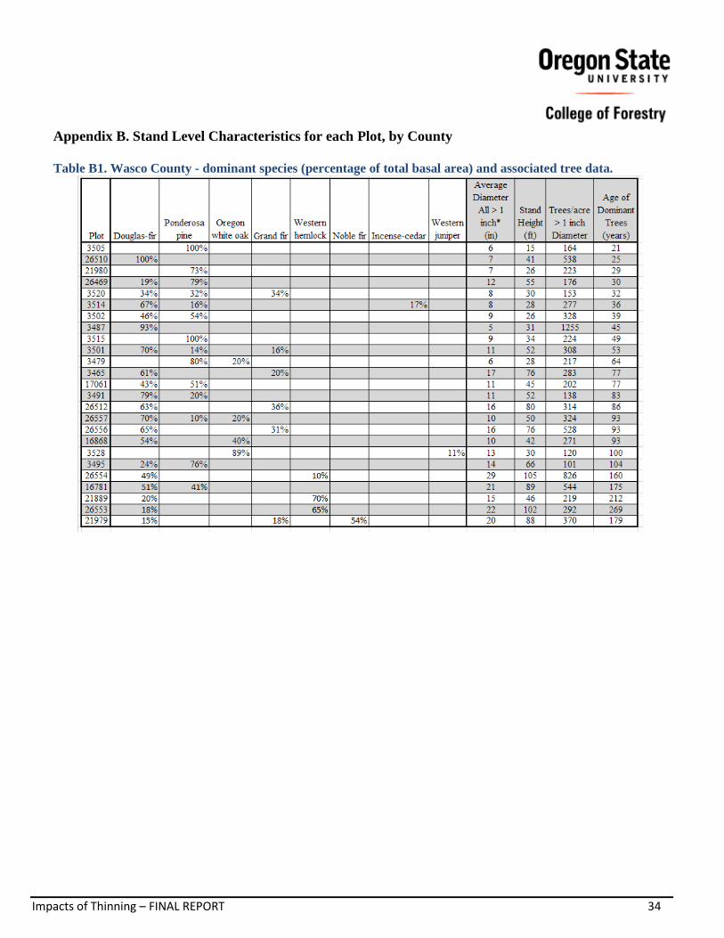
Impacts of Thinning – FINAL REPORT 34
Appendix B. Stand Level Characteristics for each Plot, by County Table B1. Wasco County - dominant species (percentage of total basal area) and associated tree data.

Impacts of Thinning – FINAL REPORT 35
Table B2. Jefferson County - dominant species (percentage of total basal area) and associated tree data.
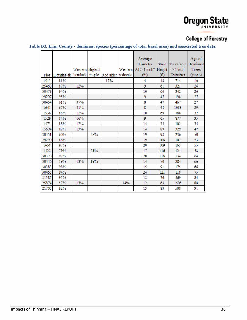
Impacts of Thinning – FINAL REPORT 36
Table B3. Linn County - dominant species (percentage of total basal area) and associated tree data.
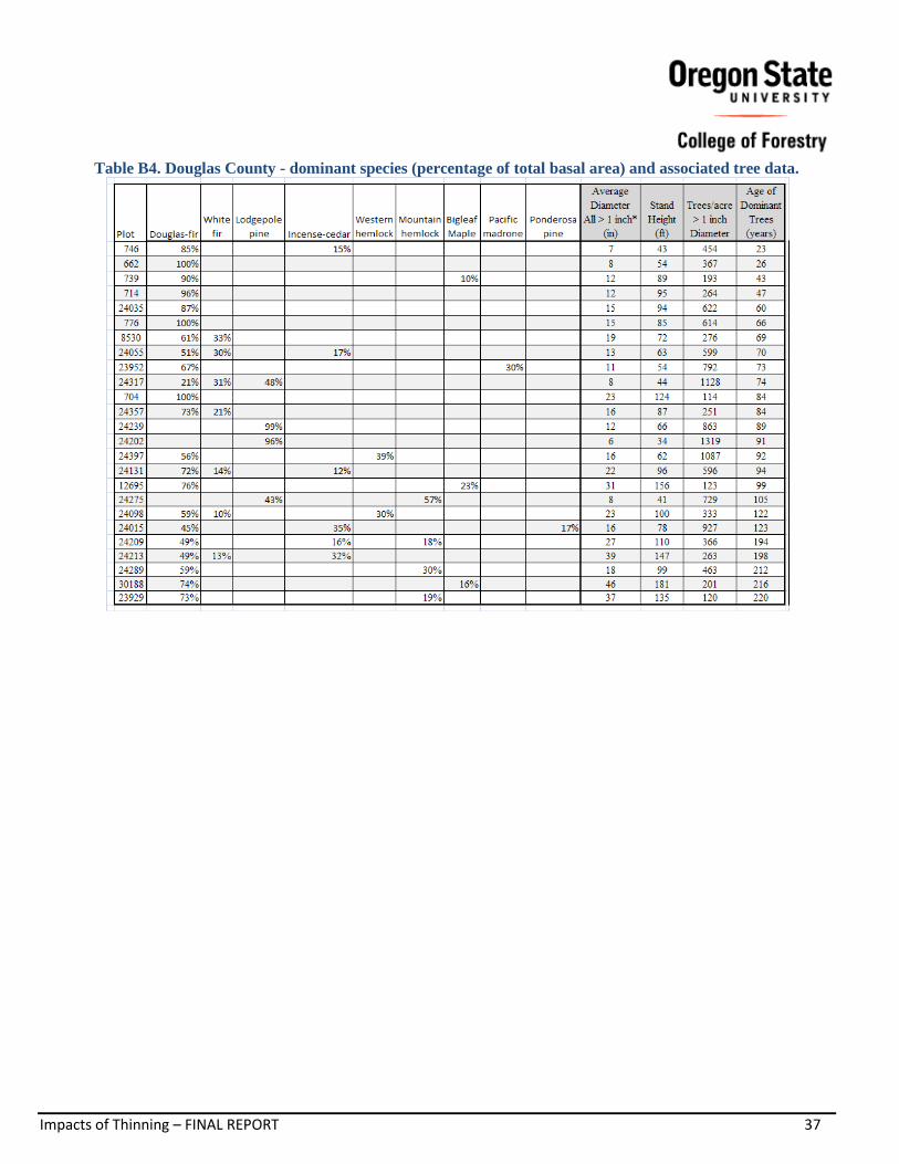
Impacts of Thinning – FINAL REPORT 37
Table B4. Douglas County - dominant species (percentage of total basal area) and associated tree data.

Impacts of Thinning – FINAL REPORT 38
Table B5. Crook County - dominant species (percentage of total basal area) and associated tree data.

Impacts of Thinning – FINAL REPORT 39
Appendix C. Understory Vegetation by County
Table C1. Most common understory vegetation for Wasco County plots.

Impacts of Thinning – FINAL REPORT 40
Table C2. Most common understory vegetation for Jefferson County plots.

Impacts of Thinning – FINAL REPORT 41
Table C3. Most common understory vegetation for Linn County plots.
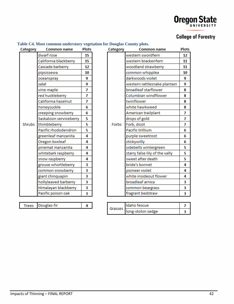
Impacts of Thinning – FINAL REPORT 42
Table C4. Most common understory vegetation for Douglas County plots.
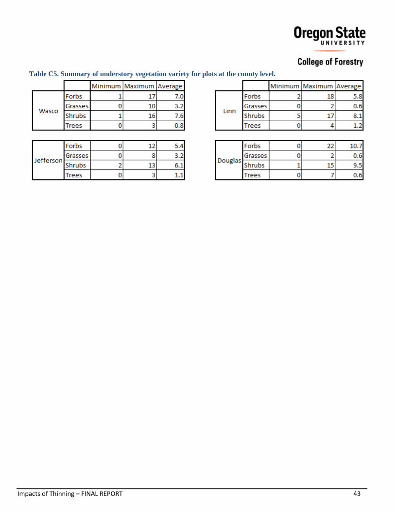
Impacts of Thinning – FINAL REPORT 43
Table C5. Summary of understory vegetation variety for plots at the county level.
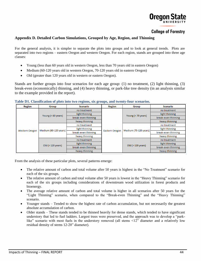
Impacts of Thinning – FINAL REPORT 44
Appendix D. Detailed Carbon Simulations, Grouped by Age, Region, and Thinning
For the general analysis, it is simpler to separate the plots into groups and to look at general trends. Plots are
separated into two regions – eastern Oregon and western Oregon. For each region, stands are grouped into three age
classes:
Young (less than 60 years old in western Oregon, less than 70 years old in eastern Oregon)
Medium (60-120 years old in western Oregon, 70-120 years old in eastern Oregon)
Old (greater than 120 years old in western or eastern Oregon).
Stands are further groups into four scenarios for each age group: (1) no treatment, (2) light thinning, (3)
break-even (economically) thinning, and (4) heavy thinning, or park-like tree density (in an analysis similar
to the example provided in the report).
Table D1. Classification of plots into two regions, six groups, and twenty-four scenarios.
From the analysis of these particular plots, several patterns emerge:
The relative amount of carbon and total volume after 50 years is highest in the “No Treatment” scenario for
each of the six groups.
The relative amount of carbon and total volume after 50 years is lowest in the “Heavy Thinning” scenario for
each of the six groups including considerations of downstream wood utilization in forest products and
bioenergy.
The average relative amount of carbon and total volume is higher in all scenarios after 50 years for the
“Light Thinning” scenario, when compared to the “Break-even Thinning” and the “Heavy Thinning”
scenario.
Younger stands – Tended to show the highest rate of carbon accumulation, but not necessarily the greatest
absolute accumulation of carbon.
Older stands – These stands tended to be thinned heavily for dense stands, which tended to have significant
understory that led to fuel ladders. Largest trees were preserved, and the approach was to develop a “park-
like” scenario with most fuels in the understory removed (all stems <12” diameter and a relatively low
residual density of stems 12-20” diameter).
Impacts of Thinning – FINAL REPORT 45
Eastern Oregon vs. western Oregon – The plots in western Oregon tended to have higher amounts of initial
carbon, and higher rates of carbon and volume accumulation. This relationship was observed for all
scenarios.
.
This set of plots does not necessarily indicate carbon levels at a regional level, and a spatial analysis should be
conducted before making broader conclusions based on these simulations.
Guide to Reading Graph Legends Average Live Carbon. Simulates aboveground carbon store of all live standing trees and shrubs/herbs. There is one
solid line that represents average simulated carbon for all plots in the given scenario (MgC/ha).
Average Total Carbon. Simulates sum of forest carbon pools estimated by FVS and allometric equations. There is
one solid line that represents average simulated carbon for all plots in the given scenario (MgC/ha).
Average Carbon Offset from not Burning Coal. When burning biomass for energy instead of coal, the carbon
emissions for biomass replaces the carbon emissions for coal. This bar includes the estimated
“avoided” carbon emissions for each thinning scenario when burning biomass for energy instead of
coal (MgC/ha).
Average Carbon stored in Wood Products- This is the estimated carbon transferred and stored in harvested wood
products for each thinning scenario (MgC/ha).

Impacts of Thinning – FINAL REPORT 46
Figure D1. Eastern Oregon – young stands. Simulation of carbon pools for the forest stand over a 50 year period. Biomass for energy is not
included in wood product sequestration – it is assumed utilized within the first year.

Impacts of Thinning – FINAL REPORT 47
Figure D2. Eastern Oregon – medium stands. Simulation of carbon pools for the forest stand over a 50 year period. Biomass for energy is not
included in wood product sequestration – it is assumed utilized within the first year.

Impacts of Thinning – FINAL REPORT 48
Figure D3. Eastern Oregon – old stands. Simulation of carbon pools for the forest stand over a 50 year period. Biomass for energy is not
included in wood product sequestration – it is assumed utilized within the first year.
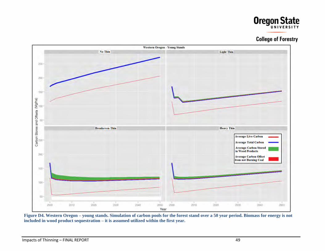
Impacts of Thinning – FINAL REPORT 49
Figure D4. Western Oregon – young stands. Simulation of carbon pools for the forest stand over a 50 year period. Biomass for energy is not
included in wood product sequestration – it is assumed utilized within the first year.
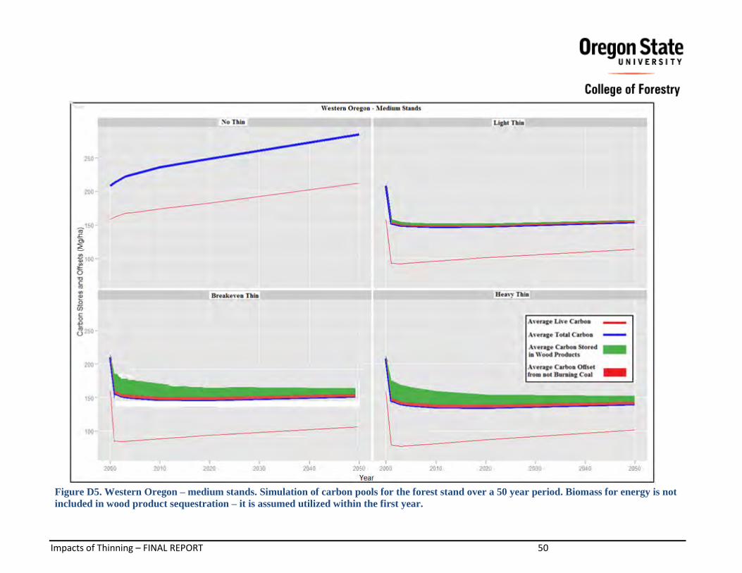
Impacts of Thinning – FINAL REPORT 50
Figure D5. Western Oregon – medium stands. Simulation of carbon pools for the forest stand over a 50 year period. Biomass for energy is not
included in wood product sequestration – it is assumed utilized within the first year.

Impacts of Thinning – FINAL REPORT 51
Figure D6. Western Oregon – old stands. Simulation of carbon pools for the forest stand over a 50 year period. Biomass for energy is not
included in wood product sequestration – it is assumed utilized within the first year.
Impacts of Thinning – FINAL REPORT 52
Appendix E. Carbon Accounting Methodology Using FVS and other Tools
There are several different methods and tools available to estimate tree-level and/or plot-level carbon. In this
analysis, the primary source for biomass and carbon estimates is the FVS-FFE extension. Two components
(1-ft stump and bole bark) were estimated manually. All plot carbon stores are included in estimates except
for soil carbon. In all components, carbon weight is estimated as 50% of bone-dry biomass weight (see page
325 Penman et al. 2003) except for litter and duff, which is estimated as 37% carbon (Smith and Heath
2002).
Most of the detailed information about FVS calculations was taken from FVS user manuals or from personal
communication with developers.
The carbon pools for each plot were estimated as follows:
Aboveground Standing Live (FVS and Allometric Estimates):
Bole Biomass (FVS):
Bole volume (green) is estimated using equations from the National Volume Estimator Library, based
on region, species, diameter at breast height (DBH), height, and other tree-level measurements.
Specific gravity for the tree species/region is used (Reinhardt et al. 2009) to estimate bole biomass
from green volume by the equation Bole Biomass = Green Volume * Specific gravity (Forest
Products Laboratory 1999).
Defects can be accounted for using total volume estimates in FVS, and 15% defect is included for
wood products estimates, as in a previous study (Adams and Latta 2003).
Bole bark is not included in the FVS estimate, but was included manually (see below).
Stump biomass (from ground to 1 foot height) were not included in FVS-FFE estimates, but they
were included manually (see below for stump calculations).
Bole Bark Biomass (Allometric Estimate):
Estimate from regional biomass estimates (Gholz et al. 1979). Estimates are based on species and DBH.
Stump Biomass (Allometric Estimate):
The stump not accounted for in the FFE-FVS measurement is 1 ft high. The part of the stump above 0.5
ft is considered part of the bole when harvested, and the part of the stump below 0.5 ft is assumed
aboveground biomass left behind if the tree is cut.
Diameter estimates for stumps are taken from allometric equations (Wensel and Olson 1995). Function
of species, DBH, height of DBH measurement.
The assumed cut height for stumps was 0.5 ft. Stump volume was estimated by dividing the 1-ft stump
into 2 frustums, each 0.5 ft high.
Density is assumed to be a constant (not height dependent) for each species (Bouffier et al. 2003;
Megraw 1985). Biomass is calculated as Density*Volume. Carbon is assumed to be 50% of bone-dry
weight.
Impacts of Thinning – FINAL REPORT 53
Crown Biomass (FVS):
Equations based on tree parameters (species, DBH, height, relative dominance in the plot). (Brown and
Johnston 1976).
Crown biomass estimates also based on crown ratio, tree height in stand.
o If ≥ 60th percentile, then assumed dominant/co-dominant.
o If < 60th percentile, then assumed suppressed/intermediate.
The crown is divided into dead/live and material size by diameter (foliage, <0.25”, 0.25”-1”, 1”-3”, >3”).
Aboveground Standing Dead (FVS):
This component was modeled based on several factors (details in Rebain 2008). Parameters modeled include
snag fall (and associated height loss) and decay rates based on several parameters, including regional
temperature, moisture class by plant association, years before hard snags become soft snags, soil moisture,
soil depth, and soil position.
All plots have dead trees that are measured and included. Snags are classified as recent mortality or not recent
mortality.
The 0.5 ft stumps left after thinning are also included. A study of decomposition rates of stumps in an old-
growth stand of Douglas-fir and western hemlock (Janisch et al. 2005) suggested that log decay rates can be
substituted for stump decay rates. In this analysis, the FVS decay rates of course woody debris are applied to
stumps. Annual decay rates are 2.5% for stumps less than 3” diameter, and 1.25% for stumps greater than 3”
diameter.
Belowground Live (FVS):
Includes all coarse roots >2mm (0.079 in) in diameter.
Fine roots are assumed to be part of soil carbon (e.g., Jenkins 2003), and are not estimated.
Belowground Dead (FVS):
Includes coarse roots >2mm (0.0079 in) in diameter. Smaller roots are not estimated.
The default root decay rate of 0.0425 is used (Ludovci et al. 2002).
Forest Floor (FVS):
Includes duff and leaf litter.
Annual litterfall uses estimates based on Keane et al. 1989, and is a function of species, foliage
weight, and leaf lifespan.
Downed Dead Wood (FVS):
For this pool, the default value is used initially (Reinhardt et al. 2009).
Shrubs and Herbs (FVS):
Does not dynamically simulate weight of shrubs and herbs, and is assumed roughly constant in a
stand, given the understory vegetation associated with a plot.
Biomass estimates are based on the First Order Fire Effects Model (FOFEM) (Reinhardt et al. 1997).

Impacts of Thinning – FINAL REPORT 54
Conversion from bone-dry biomass weight to carbon
The conversion from bone-dry biomass to carbon is simple. Carbon content for all biomass is assumed to be
50% of bone-dry biomass except for litter and duff which is estimated as 37% of bone-dry biomass.
Moisture Content
All moisture content estimates are made using wet basis. This basis estimates water content as a fraction of
green weight.
x 100.

Impacts of Thinning – FINAL REPORT 55
Appendix F. Summary Tables of Carbon Stores, Fluxes, Relative Carbon and Fuel Reduction Measurement.
Table F1. Estimated mean carbon stores with associated standard error for each region/age category. Initial growing stock volume is total
volume, not merchantable volume. Carbon pools for each plot are separated into three categories: (1) Live (Aboveground Standing,
Belowground Live, Shrubs and Herbs); (2) Dead (Belowground Dead, Standing Dead, Downed Dead Wood); and (3) Forest Floor. Data is
presented as: carbon mean [Mg/hectare] (carbon standard error) [Mg/hectare].
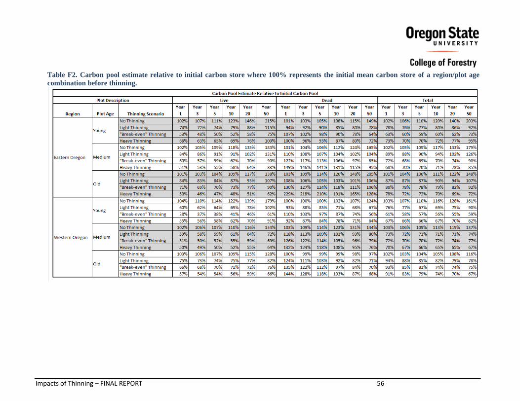
Impacts of Thinning – FINAL REPORT 56
Table F2. Carbon pool estimate relative to initial carbon store where 100% represents the initial mean carbon store of a region/plot age
combination before thinning.

Impacts of Thinning – FINAL REPORT 57
Table F3. Torching Index and Crowning Index estimates.
Torching Index is the wind speed at which crown fire is expected to initiate (based on Rothermel (1972) surface fire model and Van Wagner
(1977) crown fire initiation criteria. Crowning Index is the wind speed at which active crowning fires are possible (based on Rothermel
(1991) crown fire spread rate model and Van Wagner (1977) criterion for active crown fire spread). Wind speed refers to speed of wind
measured 20 ft above the canopy. Lower values indicate higher susceptibility. Data is presented as: crowning/torching index [mi/hr]
(standard deviation) [mi/hr] for select years. Red indicates that plots would benefit from a thinning using the criteria in this study. Orange
indicates the average was still below criteria following the thinning, and green indicates that the average index for plots was above the
minimum criteria used in this study.

Impacts of Thinning – FINAL REPORT 58
Figure F1. Torching Index (mi/hr) over a 50 year period – comparison is for different treatments for region/age combinations. This is a
graphical representation of the means (averages) from Table F3, and does not include variance, which is relatively high compared to the
mean.
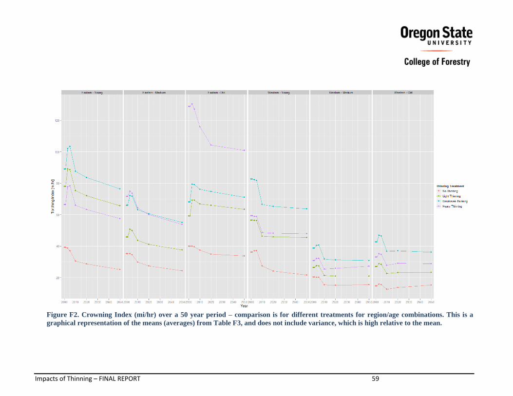
Impacts of Thinning – FINAL REPORT 59
Figure F2. Crowning Index (mi/hr) over a 50 year period – comparison is for different treatments for region/age combinations. This is a
graphical representation of the means (averages) from Table F3, and does not include variance, which is high relative to the mean.
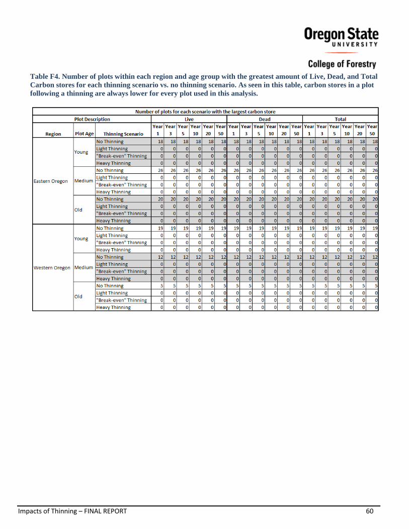
Impacts of Thinning – FINAL REPORT 60
Table F4. Number of plots within each region and age group with the greatest amount of Live, Dead, and Total
Carbon stores for each thinning scenario vs. no thinning scenario. As seen in this table, carbon stores in a plot
following a thinning are always lower for every plot used in this analysis.

Impacts of Thinning – FINAL REPORT 61
Appendix G. Conversion Units and Definitions.
Conversion factors from metric to imperial units.
1 hectare (ha) = 2.471 acre (ac)
1 meter (m) = 3.281 feet (ft)
1 square meter (m2) = 10.764 square feet (ft
2)
1 cubic meter (m3) = 35.315 cubic feet (ft
3)
1 megagram (Mg) = 1000 kilograms (kg) = 1 metric tonne = 1.102 short tons
1 short ton = 2000 pounds (lbs)
1 kilowatt-hr (kWh) = 3413 British Thermal Units (BTU)
Definitions from IPCC FAR used in this report (IPCC 2007):
Reservoir – “a component of the climate system other than the atmosphere which has the capacity to store,
accumulate or release… greenhouse gas...”
Sink – “any process, activity or mechanism that removes a greenhouse gas … from the atmosphere.”
Source – “any process, activity or mechanism that releases a greenhouse gas… into the atmosphere.”