Impacts of Model Building Energy Codes

PNNL-25611 Rev. 1

Impacts of Model Building Energy Codes

October 2016

RA Athalye B Liu D Sivaraman R Bartlett DB Elliott

PNNL-25611 Rev. 1

Impacts of Model Building Energy Codes RA Athalye B Liu D Sivaraman R Bartlett DB Elliott October 2016 Prepared for the U.S. Department of Energy under Contract DE-AC05-76RL01830 Pacific Northwest National Laboratory Richland, Washington 99352

iii

Executive Summary

The U.S. Department of Energy (DOE) Building Energy Codes Program (BECP) periodically evaluates national and state-level impacts associated with energy codes in residential and commercial buildings. Pacific Northwest National Laboratory (PNNL), funded by DOE, conducted an assessment of the prospective impacts of national model building energy codes from 2010 through 2040. A previous PNNL study evaluated the impact of the Building Energy Codes Program1; this study looked more broadly at overall code impacts. This report describes the methodology used for the assessment and presents the impacts in terms of energy savings, consumer cost savings, and reduced CO2 emissions at the state level and at aggregated levels. This analysis does not represent all potential savings from energy codes in the U.S. because it excludes several states which have codes which are fundamentally different from the national model energy codes or which do not have state-wide codes.

Energy codes follow a three-phase cycle that starts with the development of a new model code, proceeds with the adoption of the new code by states and local jurisdictions, and finishes when buildings comply with the code. The development of new model code editions creates the potential for increased energy savings. After a new model code is adopted, potential savings are realized in the field when new buildings (or additions and alterations) are constructed to comply with the new code. Delayed adoption of a model code and incomplete compliance with the code’s requirements erode potential savings. The contributions of all three phases are crucial to the overall impact of codes, and are considered in this assessment.

Figure ES.1 schematically describes the analysis framework. Energy savings are expressed in terms of energy use intensity (EUI) in the figure.

Figure ES.1. Codes Impact Analysis Framework

1 Building Energy Codes Program: National Benefits Assessment, 1992-2040. Available at: https://www.energycodes.gov/sites/default/files/documents/BenefitsReport_Final_March20142.pdf

iv

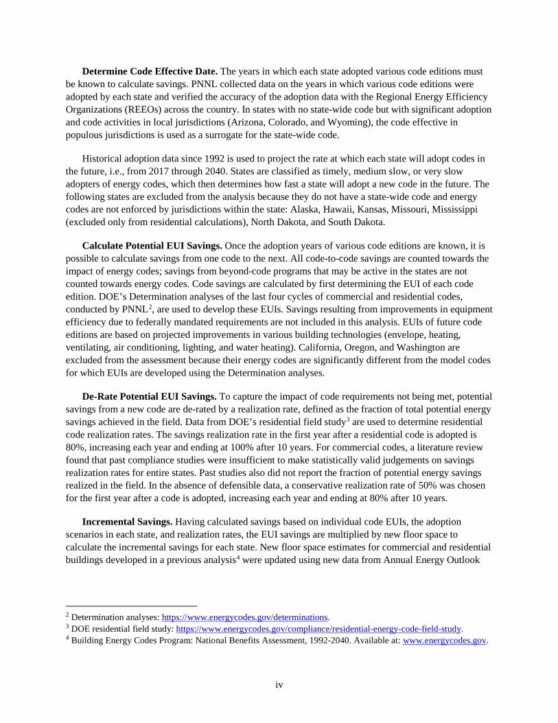
Determine Code Effective Date. The years in which each state adopted various code editions must be known to calculate savings. PNNL collected data on the years in which various code editions were adopted by each state and verified the accuracy of the adoption data with the Regional Energy Efficiency Organizations (REEOs) across the country. In states with no state-wide code but with significant adoption and code activities in local jurisdictions (Arizona, Colorado, and Wyoming), the code effective in populous jurisdictions is used as a surrogate for the state-wide code.

Historical adoption data since 1992 is used to project the rate at which each state will adopt codes in the future, i.e., from 2017 through 2040. States are classified as timely, medium slow, or very slow adopters of energy codes, which then determines how fast a state will adopt a new code in the future. The following states are excluded from the analysis because they do not have a state-wide code and energy codes are not enforced by jurisdictions within the state: Alaska, Hawaii, Kansas, Missouri, Mississippi (excluded only from residential calculations), North Dakota, and South Dakota.

Calculate Potential EUI Savings. Once the adoption years of various code editions are known, it is possible to calculate savings from one code to the next. All code-to-code savings are counted towards the impact of energy codes; savings from beyond-code programs that may be active in the states are not counted towards energy codes. Code savings are calculated by first determining the EUI of each code edition. DOE’s Determination analyses of the last four cycles of commercial and residential codes, conducted by PNNL2, are used to develop these EUIs. Savings resulting from improvements in equipment efficiency due to federally mandated requirements are not included in this analysis. EUIs of future code editions are based on projected improvements in various building technologies (envelope, heating, ventilating, air conditioning, lighting, and water heating). California, Oregon, and Washington are excluded from the assessment because their energy codes are significantly different from the model codes for which EUIs are developed using the Determination analyses.

De-Rate Potential EUI Savings. To capture the impact of code requirements not being met, potential savings from a new code are de-rated by a realization rate, defined as the fraction of total potential energy savings achieved in the field. Data from DOE’s residential field study3 are used to determine residential code realization rates. The savings realization rate in the first year after a residential code is adopted is 80%, increasing each year and ending at 100% after 10 years. For commercial codes, a literature review found that past compliance studies were insufficient to make statistically valid judgements on savings realization rates for entire states. Past studies also did not report the fraction of potential energy savings realized in the field. In the absence of defensible data, a conservative realization rate of 50% was chosen for the first year after a code is adopted, increasing each year and ending at 80% after 10 years.

Incremental Savings. Having calculated savings based on individual code EUIs, the adoption scenarios in each state, and realization rates, the EUI savings are multiplied by new floor space to calculate the incremental savings for each state. New floor space estimates for commercial and residential buildings developed in a previous analysis4 were updated using new data from Annual Energy Outlook

2 Determination analyses: https://www.energycodes.gov/determinations. 3 DOE residential field study: https://www.energycodes.gov/compliance/residential-energy-code-field-study. 4 Building Energy Codes Program: National Benefits Assessment, 1992-2040. Available at: www.energycodes.gov.

https://www.energycodes.gov/determinations

https://www.energycodes.gov/compliance/residential-energy-code-field-study

http://www.energycodes.gov/

v

2015.5 New floor space added each year includes new construction, additions, and, for commercial buildings only, alterations.

Annual and Cumulative Savings. Projected impacts are reported in terms of annual savings in a given year, as well as cumulative savings for different periods. The terms annual and cumulative are described in greater detail in section 2.2.

Table ES.1 summarizes the impact of energy codes beginning in 2010 and ending in 2040 for all states included in the analysis. The results include savings from electricity, natural gas, and fuel oil (residential only) and are reported separately for residential and commercial codes. The cumulative primary energy savings from 2010-2040 are 12.82 quads. In terms of financial benefits to consumers from reduced utility bills, energy codes could save $126 billion dollars from 2010 to 2040. This equates to a CO2 reduction of 841 million metric tons (MMT). These savings are approximately equal to the greenhouse gases emitted by 177 million passenger vehicles driven for one year or the CO2 emissions from 245 coal power plants for one year6.

Table ES.1. Summary of Impact of Energy Codes

Sector

Site Energy Savings (Quads)

Primary Energy Savings (Quads)

Full-Fuel-Cycle

Savings (Quads)

Energy Cost

Savings (2016 $ billion)

CO2 Reduction

(MMT) Commercial

Annual 2030 0.10 0.26 0.28 2.24 17.57 Annual 2040 0.13 0.32 0.34 2.54 21.48 Cumulative 2010-2030 1.18 3.14 3.30 27.53 208.78 Cumulative 2010-2040 2.34 6.10 6.41 51.59 405.51

Residential Annual 2030 0.15 0.28 0.30 3.14 18.38 Annual 2040 0.17 0.33 0.35 3.45 21.46 Cumulative 2010-2030 1.87 3.62 3.86 41.19 234.52 Cumulative 2010-2040 3.48 6.72 7.17 74.34 435.43

Total Annual 2030 0.25 0.55 0.58 5.37 35.96

Annual 2040 0.30 0.66 0.69 5.98 42.93 Cumulative 2010-2030 3.06 6.76 7.16 68.72 443.30 Cumulative 2010-2040 5.82 12.82 13.58 125.93 840.94

Note: The following states are excluded from the analysis: AK, CA, HI, KS, MO, MS (residential only), ND, OR, SD, and WA. See section 2.1.3 for details.

5 Energy Information Administration’s Annual Energy Outlook projects new floor space added in the future. Accessed at: http://www.eia.gov/forecasts/aeo/. 6 EPA’s Greenhouse Gas Equivalencies Calculator: https://www.epa.gov/energy/greenhouse-gas-equivalencies-calculator

http://www.eia.gov/forecasts/aeo/

https://www.epa.gov/energy/greenhouse-gas-equivalencies-calculator

https://www.epa.gov/energy/greenhouse-gas-equivalencies-calculator

vi

Acknowledgments

The authors would like to thank David Cohan and Jeremy Williams of the Department of Energy for their guidance and oversight throughout the completion of this assessment. The authors would also like to thank Isaac Elnecave (MEEA), Ken Baker (NEEA), Darren Port and Carolyn Sarno (NEEP), Lauren Westmoreland (SEEA), Richard Morgan (SPEER), Jim Myers (SWEEP), and Allen Lee (Cadmus) for providing assistance during the assessment and reviewing the report. A special thanks to Lowell Ungar of ACEEE who served as a sounding board for ideas on the methodology. The authors appreciate the contributions of PNNL staff including Todd Taylor, Vrushali Mendon, Pam Cole, Mingjie Zhao, Jian Zhang, and Mike Rosenberg.

vii

Acronyms and Abbreviations

ACEEE American Council for an Energy-Efficient Economy AEO Annual Energy Outlook AIA American Institute of Architects BECP Building Energy Codes Program BTO Building Technologies Office Btu British Thermal Unit DHW Domestic Hot Water DOE Department of Energy ECPA Energy Conservation and Production Act EIA Energy Information Administration EUI Energy Use Intensity FFC Full-Fuel Cycle ICC International Code Council IECC International Energy Conservation Code LED Light Emitting Diode LEED Leadership in Energy and Environmental Design MEEA Midwest Energy Efficiency Alliance MMT Million Metric Tons NEEA Northwest Energy Efficiency Alliance NEEP Northeast Energy Efficiency Partnerships NEMS National Energy Modeling System NIA National Impact Analysis NOMAD Naturally Occurring Market Adoption PNNL Pacific Northwest National Laboratory REEO Regional Energy Efficiency Organization SEEA Southeast Energy Efficiency Alliance SPEER South-central Partnership for Energy Efficiency as a Resource SWEEP Southwest Energy Efficiency Project SWH Service Water Heating

ix

Contents

Executive Summary .......................................................................................................................... iii Acknowledgments .............................................................................................................................. vi Acronyms and Abbreviations ...........................................................................................................vii 1.0 Introduction ................................................................................................................................ 1 2.0 Methodology ............................................................................................................................... 3

2.1 Analysis Framework .......................................................................................................... 3 2.1.1 Scope of Analysis .................................................................................................... 4 2.1.2 Rolling Baseline Approach ..................................................................................... 5 2.1.3 Code Effective Date ................................................................................................ 6 2.1.4 Code-to-Code Savings ............................................................................................. 6 2.1.5 Savings Realized in the Field .................................................................................. 8 2.1.6 Floor Space Multiplier ............................................................................................ 9

2.2 Calculation of Incremental, Annual, and Cumulative Savings .......................................... 9 2.3 Sample Calculation .......................................................................................................... 10

3.0 Results ...................................................................................................................................... 12 4.0 References ................................................................................................................................ 21 Appendix A – Model Inputs ........................................................................................................... A.1 Appendix B – Site Energy Savings By Fuel Type .......................................................................... B.1 Appendix C – Maximum Potential Savings .................................................................................... C.1

x

Figures

ES.1 Codes Impact Analysis Framework ............................................................................................ iii 1 Codes Impact Analysis Framework ............................................................................................ 4 2 Incremental Savings Calculation ................................................................................................. 4

Tables

ES.1 Summary of Impact of Energy Codes ......................................................................................... v 1 With No Mandatory State-wide Code or Enforcement Restrictions ........................................... 5 2 Example Calculation of Incremental, Annual, and Cumulative Savings for One State .............. 11 3 Summary of Energy Codes Impact ............................................................................................. 13 4 Site Energy Savings (TBtu) ........................................................................................................ 14 5 Primary Energy Savings (TBtu) .................................................................................................. 15 6 FFC Energy Savings (TBtu) ........................................................................................................ 16 7 Discounted Consumer Cost Savings (Billion $ 2016)................................................................. 17 8 Avoided CO2 Emissions (MMT) ................................................................................................. 18 9 Annual and 5-Year Cumulative Savings ..................................................................................... 19 10 Impact of Codes from 2010-2016 ............................................................................................... 20 A.1 Commercial Codes Adoption Classification by State ................................................................. A.2 A.2 Residential Codes Adoption Classification by State ................................................................... A.4 A.3 Commercial Future Code Edition Energy Reduction Factors (90.1-2013 = 1.00) ...................... A.6 A.4 Residential Future Code Edition Energy Reduction Factors (2015 IECC = 1.00) ...................... A.7 A.5 Future Code Edition Savings ...................................................................................................... A.7 A.6 Commercial Floor Space Scaling Factors 2011-2014 ................................................................. A.8 A.7 Residential Stock Survival Factors ............................................................................................. A.8 B.1 Electricity Site Energy Savings by State (TBtu) ......................................................................... B.1 B.2 Natural Gas Site Energy Savings by State (TBtu) ...................................................................... B.2 B.3 Fuel Oil Site Energy Savings by State (TBtu) ............................................................................ B.3 C.1 Summary of Energy Codes Impact with 100% Compliance ....................................................... C.1

1

1.0 Introduction

Building energy codes regulate the energy efficiency of new construction and major renovations of buildings. Energy codes have been in place in one form or another since the 1970s and became part of official federal policy in 1992 with the amendment1 of the Energy Conservation and Production Act (ECPA). The U.S. Department of Energy’s (DOE’s) Building Energy Codes Program (BECP) was created in response to congressional direction in ECPA to promote energy efficiency in buildings through energy codes. Since then, BECP has supported the development and adoption of model energy codes, and encouraged compliance with those codes through various educational and tool-development activities.

Model codes are codes developed by a national consensus process and made available for adoption by states and local jurisdictions. The model codes of interest in this report are the International Energy Conservation Code (IECC)2 for residential and ASHRAE Standard 90.13 for commercial as these are explicitly referenced in the amended provisions of ECPA and are the basis for the vast majority of U.S. state codes.

The most recent three editions of the IECC and ASHRAE Standard 90.1 have the potential to generate almost a 30% reduction in energy use compared to codes a decade ago (Halverson et al. 2014, Mendon et al. 2015). Together with this rapid progress of codes in the recent past, the President’s Climate Action Plan and the Clean Power Plan have generated increased interest in understanding the magnitude of the impact of energy code activities as a whole.

To respond to this interest, PNNL, funded by DOE’s Building Energy Codes Program, conducted an assessment of the national impact of building energy codes from 2010-2040. This report describes the methodology and presents the results of the assessment. The starting point of 2010 is chosen because it coincides with the start year for the goals established in the DOE Building Technologies Office’s (BTO) Multi-Year Program Plan (BTO 2016). The current assessment builds upon previous analysis, through which PNNL evaluated the historical impacts of buildings energy codes from1992 through 2010 (Livingston et al. 2014).

The start year of the analysis is a sensitive input. Codes have been in existence since the 1970s and the BECP has been in existence since 1992. Buildings constructed earlier than 2010 and complying with earlier codes have been generating savings and will continue to generate savings in the future. By picking the start year as 2010, savings from the previous years are not reflected in this assessment. If the start year were 1992, for example, savings accrued in 2010 and future years would increase significantly. Thus, the overall impact of energy codes in this assessment can be considered conservative. This is particularly true because the analysis does not include potential savings from states whose energy codes are fundamentally different from the national model energy codes and states which have neither a state-wide code nor significant adoption and enforcement activities by local jurisdictions.

1 Energy Conservation and Production Act (Pub. L. No. 94-385), as amended by the Energy Policy Act of 1992 (Pub. L. No. 102-486). 2 See www.iccsafe.org. 3 See www.ashrae.org.

http://www.iccsafe.org/

http://www.ashrae.org/

2

Section 2.0 of this report describes the overall technical approach. Results are presented in Section 3.0. Appendix A provides details on the inputs used in the assessment. Appendix B provides further breakdown of the energy savings results by fuel type. Appendix C shows the impact of codes if all the potential savings from a code were realized in the field.

3

2.0 Methodology

Model energy codes follow a three-phase cycle that starts with the development of a new model code, continues with the adoption of the new code by states and local jurisdictions, and finishes when newly constructed buildings are required to comply with the new code. The contribution of all three phases on the overall impact of the code is considered in this assessment. Once a new model code is developed, states need to take action to formally adopt the new code. After the new code is adopted, savings4 are realized in the field only when new buildings (or additions and alterations) are constructed to comply with the new code. Delayed adoption of a new model code and incomplete compliance with all the code’s requirements erode potential savings.

This analysis uses a “rolling baseline” in which savings are based on the difference in energy efficiency between a new code and its immediate predecessor. When a new code is adopted, the version it replaced becomes the baseline against which savings are calculated. This changes with each new code, thus a “rolling baseline.” A detailed discussion about the rolling baseline can be found in section 2.1.2.

In this analysis, potential savings between one code and its successor do not include savings resulting from improvements in equipment efficiency mandated by federal rulemakings. DOE rulemakings set minimum efficiency levels for certain heating, ventilating, and air conditioning (HVAC), and service water heating (SWH) equipment. These improvements in equipment efficiency would result regardless of whether a new code is enforced, and are therefore not attributable to the energy code.

There are many beyond-code programs, such as utility incentive programs, Energy Star (EPA 2016), LEED (USGBC 2016), as well as other locally- and state-funded programs that promote energy efficiency in buildings. Such programs have an impact on the energy efficiency of the building stock that can be considered separate from the code impact. For example, the first phase of the DOE residential field study (BECP 2016a) showed that windows installed in new homes consistently and significantly exceeded code requirements in all participating states. This higher level of window performance might be driven by certain beyond-code programs but it is very difficult to separate the impact of these programs from the impact of codes. Energy codes remain the primary mechanism through which improvements in energy efficiency are enforced on the majority of the building stock. In this analysis, potential improvement between successive codes is entirely attributed to the new code. No credit is taken for improvements beyond the requirements within the energy code.

2.1 Analysis Framework This section describes the analytical framework of the assessment and provides further detail on how

the savings calculation is structured. Figure 1 provides a schematic overview of the framework. The assessment begins with the adoption of codes at the state level starting in 2010. In each year, potential savings are calculated by subtracting the energy use intensity (EUI) of the current code from the EUI of the previous code. Next, potential savings are de-rated by realization rate to determine savings realized in the field. Finally, the de-rated savings are multiplied by the floor space added in a given year to calculate the incremental savings in that year (Figure 2). The process repeats each year starting with the evaluation of the code currently in place and the code that was in place before. Annual and cumulative savings are 4 Assuming the new code is more stringent than the previous code per DOE’s Determination (https://www.energycodes.gov/determinations).


4

calculated from incremental savings to determine the overall impact. More details on the calculation are provided in the following sections.

Figure 1. Codes Impact Analysis Framework

Figure 2. Incremental Savings Calculation

2.1.1 Scope of Analysis

This cannot be considered a full national analysis because several states were excluded for one of two reasons:

1. They do not adopt a code at the state level, or a state-wide code exists but it is not mandatory or there are special restrictions on enforcement. States in this category are Alaska, Hawaii, Kansas, Missouri, Mississippi (residential only), North Dakota, and South Dakota. Conversely, Arizona, Colorado, and Wyoming do not enforce state-wide codes, but their largest jurisdictions have adopted recent energy codes so they are included and treated as if they have state-wide codes in this study. Table 1 provides details on the treatment of states with no mandatory state-wide codes or enforcement.

2. They have energy codes significantly different in format and content than ASHRAE 90.1 or the IECC model codes, so the EUIs developed for this analysis could not be applied to their energy codes. Developing custom EUIs for these states was beyond the scope of this analysis. California, Oregon, and Washington are in this category. Florida previously had a highly-customized state code, but recently moved to a code based on the 2012 IECC and is therefore included in the analysis. Detailed information on adoption inputs can be found in Appendix A.

5

Table 1. With No Mandatory State-wide Code or Enforcement Restrictions

State

Mandatory Enforcement

of State-wide Code Restrictions

Use of Populous Jurisdictions or Cities as Surrogate for State-wide

Code

Alaska Yes

Commercial: only buildings in the transportation, public facilities, and education department are regulated. Residential: Must comply with state code if state financial assistance is used in construction. No

Arizona No

Yes (Phoenix, Tucson)

Colorado No

Yes (Denver, Aurora, and Boulder County)

Hawaii Yes Only enforced for commercial and residential structures over three stories in height. No

Kansas No

No Missouri No

No

Mississippi (residential only) No No North Dakota No

No

South Dakota No

No

Wyoming No Yes (Jackson and Cheyenne Counties)

Taken together, the excluded states account for 19.5% of new commercial floor space and 16.1% of new residential floor space projected to be constructed between 2011 and 2040 in the United States. While developing associated savings estimates would require EUIs that don’t currently exist, it is safe to say that the overall national impact of building energy codes is substantially higher than the results reported in this study.

2.1.2 Rolling Baseline Approach

The rolling baseline used in this study assumes the predecessor code of each newly adopted code as the baseline for savings analysis. Alternatively, a fixed baseline would assume that the first code in the study period – the one in place in a state in 2010 in this study – was the baseline for all future codes. Since this study uses the difference between the baseline EUI and the current code EUI to determine savings, it is clear that the rolling baseline results in much smaller, more conservative savings estimates. However, the fixed baseline approach was rejected as overly optimistic because it implicitly assumes that building efficiency never increases in the absence of changes to the energy code. Given a variety of market drivers for efficiency that are known to exist (product competition, utility rebates, above-code programs, etc.) that assumption was deemed insupportable.

A third approach, used in some past analyses from BECP as well as other organizations’ code impact studies, is to assume an increasingly efficient baseline intended to represent “normally occurring market adoption” (NOMAD) of efficiency in the absence of codes improvements. Assumptions about NOMAD levels are typically based on expert opinion and are thus inherently subjective, ranging from high to low depending on individual beliefs about how much efficiency will improve over time.

6

More important for the current study, a NOMAD baseline is unrelated to code development and adoption that have actually occurred. Code adoption, code-to-code savings, and compliance rates in the presence of codes are known in many cases. Relying on what is known for developing the baseline makes the analysis more robust and defensible. At the same time, all assumptions about future code levels are ultimately subjective; in the absence of a perfect way to predict the future, this study opted for the approach most closely tied to the development/adoption/implementation cycle.

It should be noted that an inherent consequence of choosing the predecessor code as the baseline is that a state that adopt codes in a timely fashion could save less energy than a state that delays new code adoption if the new code edition saves less than the previous code. This effect is discussed in greater detail in Section 3.0.

2.1.3 Code Effective Date

For this analysis, savings are generated for the first time when a state adopts a code newer than the one in place in 2010. A code was considered to be in place in a given year if the code was effective on or before July 1st of that year5. For future code adoptions, states are classified into four categories based on their historical rate of adoption:

1. Timely: State adopts new code within one code cycle. Future adoption lag = 1 year.

2. Medium Slow: State adopts new code within two code cycles. Future adoption lag = 4 years.

3. Very Slow: State adopts new code after two code cycles. Future adoption lag = 7 years.

4. Not Applicable: States with no state-wide code, no code enforced in jurisdictions within the state or with minimal relationship to the national model codes.

Based on the above classification, the year in which a state is expected to adopt a future code depends on the adoption lag and the code year. For example, Illinois, classified as timely, is anticipated to adopt the 2018 IECC in the year 2019 (a one year lag). The code year for both residential and commercial is the IECC year (and not the year in which the code book is published). For example, the code year for the 2015 IECC is 2015 even though the 2015 IECC was published in 2014. The commercial code year is based on the IECC and not on 90.1 because most states adopt the IECC (to which 90.1 is an alternate compliance path).

2.1.4 Code-to-Code Savings

Once the code in place in a given year for each state is known or assigned, code-to-code savings can be calculated by subtracting the EUI of the new code from that of the previous code. The delta between the code EUIs is used in determining the potential EUI savings in Figure 2. Code EUIs are developed using the process established by DOE for its statutorily-directed “Determinations” that indicate whether a new code will improve energy efficiency in buildings. The most recent commercial and residential determinations and their associated technical reports describe the process in greater detail (Halverson et

5 Effective dates for existing codes were based on the information available as of April 1, 2016. Any code adoption actions taken by states after that date are not included in this analysis. For example, if a state announced in May 2016 that it would adopt the 2015 IECC in 2017, this action is not included in the report.

7

al. 2014, Mendon et al. 2015). The Determination process excludes savings resulting from improvements in equipment efficiency due to federally mandated requirements. Past analyses conducted by PNNL in support of BECP, such as the long-term state benefits analysis for Standard 90.1-2013 (commercial) (ASHRAE 2013) and the cost-effectiveness analysis of the 2015 IECC (residential) (ICC 2015), which used the Determination approach, were leveraged to create the EUIs used in this analysis. Further detail on how commercial and residential EUIs are developed is provided below.

Commercial Code EUIs. There are four editions of ASHRAE Standard 90.1—2004, 2007, 2010, and 2013—for which PNNL determined EUIs. As part of the long-term benefits analysis for 90.1-2013, the Determination method was used to calculate the EUI in each state for 90.1-2013 and 90.1-2010. Simulations were performed for each climate zone in every state and the results were weighted by forecasted new construction area to produce state-level EUIs. These results are used in this analysis.

Previous Determination analyses for 90.1-2007 and 90.1-2004 could not be used directly to obtain EUIs for those Standards because when those analyses were performed, the federally mandated equipment efficiencies differed from when the Determination analysis for 90.1-2013 was conducted. To correctly calculate the EUIs for 90.1-2007, savings percentages between 90.1-2010 and 90.1-2007 calculated in the Determination analysis of 90.1-2010 are applied to the state-level EUIs of 90.1-2010. A similar process is followed to determine EUIs for 90.1-2004. This process of using savings percentages ensures that the EUIs of the four 90.1 editions (2004 through 2013) are consistent with each other in terms of the published Determination savings. EUIs for codes older than 90.1-2004 are calculated using a historical index of commercial code improvements developed by PNNL (BTO 2016).

To develop EUIs for future code editions (90.1-2016 and onwards), PNNL examined BTO’s Technology Roadmap reports for envelope, lighting, HVAC and SWH (BTO 2015, 2014a,b,c). PNNL also reviewed AIA’s 2030 Goal (AIA 2030) and the goals set by the Standard 90.1 development committee for each edition. Appendix A provides a more detailed discussion of future code EUIs. Standard 90.1-2013 achieved a 7.6% reduction over 90.1-2010, and a savings goal of approximately 5-10% better than the 2013 edition was set for the 2016 edition of Standard 90.1.

Based on this information, PNNL elected to use 5% as the reduction in EUI for the next cycle of commercial codes (90.1-2016 and 2018 IECC). Beyond the next cycle, it is difficult to predict the increases in stringency. Different reduction percentages are applied to different end-uses depending on the projected technological progress. The plug and process end-use is conservatively projected to see no reduction at all in future code editions. The impact of renewable technologies is not included in future code editions. After applying reduction percentages to end-uses, the overall reduction per cycle is between 4% and 5% (including plug loads). Detailed inputs for historical and future code edition efficiency levels can be found in Appendix A.

States can adopt either the commercial IECC or the corresponding 90.1 Standard—both are updated every three years. Each edition of the IECC has historically allowed the corresponding 90.1 edition as an alternate compliance path, and it is assumed that that practice will continue. In this analysis, the EUIs developed for 90.1 are used to represent corresponding editions of 90.1 and the IECC, because equivalent EUIs for the IECC are not available and their development is beyond the scope of this analysis. For example, 90.1-2010 and 2012 IECC are represented by a single state-level EUI.

8

States often amend certain sections of the IECC or 90.1 when adopting the code. Such amendments to commercial codes are not factored into the EUIs used in this analysis.

Residential Code EUIs. PNNL used the EUIs developed for four editions of the residential IECC—2006, 2009, 2012, and 2015—as part of the state cost-effectiveness analysis (Mendon et al. 2016). EUIs from the past analysis are used in the current assessment. The impact of state-specific code amendments were not incorporated into the EUI analysis because amended code EUIs were not available for all code editions adopted by a particular state. Plug loads are not currently regulated by residential codes and are therefore not included in the analysis.

As with the commercial codes, EUIs of future editions of residential codes are determined by reviewing BTO’s Technology Roadmaps. In recent editions, the 2015 IECC saved less than 1% relative to the 2012 version (Mendon et al. 2015) but the 2012 version saved 24% relative to the 2009 and the 2009 saved 11% relative to the 2006 (Lucas et al. 2013). Based on this information, a 5% reduction is chosen for the 2018 IECC compared to the 2015 IECC. For future code editions, different reduction percentages are applied to different end-uses depending on the projected technological progress. This results in approximately 4% to 5% reduction in EUI per cycle for future code editions. Further details on the historical and future code edition efficiency levels can be found in Appendix A.

2.1.5 Savings Realized in the Field

Energy code compliance is crucial to realizing the savings potential embedded within code requirements. While many past studies have attempted to quantify compliance with residential and commercial codes, a literature survey of past commercial compliance studies (Bartlett et al. 2016) found several problems including too-small sample sizes, sample bias, difficulty in accessing compliance documentation, and most importantly in the context of this analysis, the lack of a uniform definition of compliance. Past field studies measured the percent of requirements complied with relative to the total number of requirements, a metric aligned with how building officials see compliance but not tied to energy savings. The current analysis defines compliance as a savings realization rate equal to the fraction of the total potential savings that is achieved in the field. The savings realization rate determined in this manner is used to calculate the incremental savings in a given year, as shown in Figure 2.

DOE is currently conducting a residential field study designed to determine whether an investment in building energy code education, training, and outreach programs can produce a significant and measurable change in residential building energy savings realized in the field (BECP 2016a). This field study takes into account the sample size required to make statistically significant statements about the energy savings potential realized in the field at the state level. One of the study outcomes is a comparison of the observed EUI for an entire state with that of a hypothetical sample that fully complies with the code. Using these results, it is possible to determine the fraction of EUI savings realized in the field.

The results from the first phase of the residential field study show that states realized more than 100% of expected savings for codes that had been adopted at least two years after they had been published. Of the eight states in the field study, the seven with 2012 IECC or 2009 IECC had savings realization rates over 100%. Only one state had adopted the 2015 IECC, which was published just one year prior to adoption and measurement in the field study, and its realization rate was 89%. Based on the limited data in the field study, PNNL hypothesized that a relationship could be established between the publication date of the code and the savings realization rate—the longer the delay in adopting a code, the higher the

9

realization rate. For example, if a state adopted the 2009 IECC in the year 2015, the realization rate in 2015 would be very close to 100%. However, if a state adopted the 2015 IECC in 2016, the realization rate would be lower. The underlying theory is that the savings realized in the field seem to depend more on the time that has passed since the code was published than on the time passed since the code was adopted. Based on this hypothesis, a realization rate of 80% was chosen as a conservative estimate in the first year after the code is published. The realization rate was then increased asymptotically every year, approaching 100% at the end of 10 years. When a new code becomes effective, for example five years after the previous code, the realization rate is reset to 80% for Year 1 of the new code. This approach was applied to all residential codes and states.

Similar data for savings realized in the field in commercial buildings is not available. DOE is in the process of launching a commercial codes field study to better understand the fraction of potential savings realized from codes in commercial buildings. A pilot study conducted by PNNL (Rosenberg et al. 2016) analyzed lost energy savings from a sample of nine small office buildings in the Pacific Northwest region. The study found the maximum fraction of lost energy savings to be approximately 12%, or in other words, the lowest savings realization rate was 88%. For this analysis, a very conservative realization rate of 50% is chosen for the first year after the commercial code is published, i.e., only 50% of the potential savings are realized in the first year. For example, timely states with a future adoption time lag of one year will realize only 50% of the savings from the new code in the first year. The realization rate then increases asymptotically every year, approaching 80% in year 10. This approach is applied to all commercial codes and states.

2.1.6 Floor Space Multiplier

The incremental savings depend upon the amount of new floor space in the state that is built to the code. New floor space constructed in a given year is used to determine the incremental savings in a given year, as shown in Figure 2. Estimates of new residential and commercial floor space constructed each year were developed in a previous analysis (Livingston et al. 2014), which melded several datasets to develop a continuous stream of historical and projected annual floor space construction from 1992 through 2040. Projections were based on Census division-level floor space data from the 2012 edition of the Energy Information Administration’s (EIA) Annual Energy Outlook (AEO). The AEO provides projections of U.S. energy markets and serves as a reference for performing future energy and economic analyses.

The same methodology from the previous analysis is used to update floor space data for this analysis, with the underlying data from the 2015 edition of the AEO (EIA 2015) used to develop projections. Adjustments are made to the commercial and residential floor space streams based on the AEO 2015 data. Appendix A provides a detailed description of the changes to the floor space calculation.

Shrinkage of savings over time because of floor space demolition is not included in the analysis because it is assumed that the average lifespan of a building is longer than the length of this analysis (buildings built in 2011 will last beyond 2040).

2.2 Calculation of Incremental, Annual, and Cumulative Savings

Figure 1 and Figure 2 describe how incremental savings in a single year are calculated. Savings from code adoptions are generated throughout a building’s life because in the absence of a new code, the

10

building would have been built to an older, less energy efficient code and would have consumed more energy every year of its life. Thus, buildings built in the past are still generating savings today. Savings from past code adoptions add to the savings generated from new construction in a given year. In this analysis, three different types of savings are calculated and tabulated for each year in the study:

1. Incremental savings: Savings accruing only from new floor space added in a given year. These savings are simply a product of the code-to-code savings in a given year and the floor space added in that year.

2. Annual savings: Savings accruing from not only new floor space added in the given year but also from previous code adoptions and new floor space construction that occurred in the study period up to that year. Annual savings account for code actions that affected floor space added in previous years, and that continues to generate savings in the current year.

3. Cumulative savings: The sum of annual savings over all the years in the study period.

Savings reduction occurring from degradation of energy saving features over time is ignored for this analysis. For example, lighting occupancy sensor control savings could reduce over time because of degrading electronic components (relays, sensors, etc.) or there may be an increase in infiltration due to wear and tear of the envelope. These effects are ignored in the analysis because they will equally affect the new code and the baseline, thus having a negligible net effect on the savings. A sample calculation in the next section attempts to explain the savings calculation for a single state.

2.3 Sample Calculation

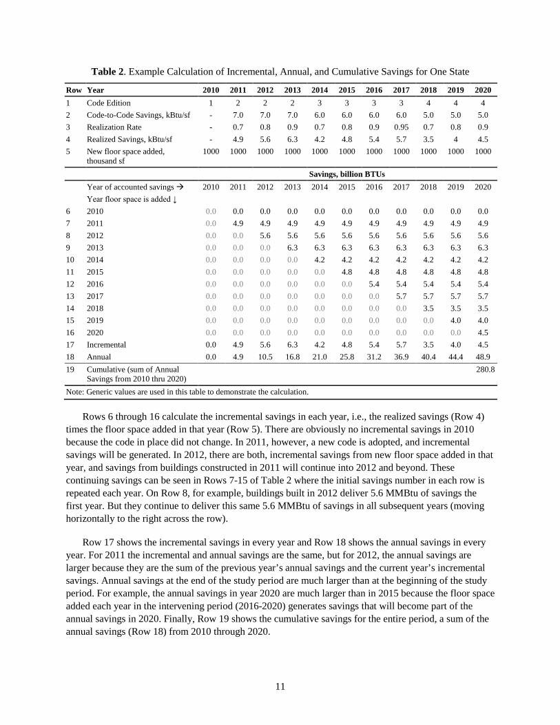
Table 2 gives an example of how incremental, annual and cumulative savings are calculated in this analysis. The calculation is performed for energy savings only for a single state for the period beginning in 2010 and ending in 2020. For simplicity, generic values are chosen for code-to-code savings, savings realization rates, and the amount of floor space added each year. Row 1 indicates the code edition. The calculation starts with code edition 1 in place in 2010. In 2011, a new code is adopted giving rise, for the first time, to energy savings indicated in row 2. These energy savings arise from the fact that code edition 2 has a higher efficiency level compared to code edition 1. Row 3 shows the savings realization rate. Note that it improves each year a code is in place and then gets lower whenever a new code is adopted. Row 4 shows the realized savings, calculated as code-to-code savings (Row 2) times the realization rate (Row 3). Row 5 shows the floor space added in a given year, which, for this example, is assumed to be a million square feet (sf) every year.

11

Table 2. Example Calculation of Incremental, Annual, and Cumulative Savings for One State

Row Year 2010 2011 2012 2013 2014 2015 2016 2017 2018 2019 2020 1 Code Edition 1 2 2 2 3 3 3 3 4 4 4 2 Code-to-Code Savings, kBtu/sf - 7.0 7.0 7.0 6.0 6.0 6.0 6.0 5.0 5.0 5.0 3 Realization Rate - 0.7 0.8 0.9 0.7 0.8 0.9 0.95 0.7 0.8 0.9 4 Realized Savings, kBtu/sf - 4.9 5.6 6.3 4.2 4.8 5.4 5.7 3.5 4 4.5 5 New floor space added,

thousand sf 1000 1000 1000 1000 1000 1000 1000 1000 1000 1000 1000

Savings, billion BTUs Year of accounted savings 2010 2011 2012 2013 2014 2015 2016 2017 2018 2019 2020 Year floor space is added ↓ 6 2010 0.0 0.0 0.0 0.0 0.0 0.0 0.0 0.0 0.0 0.0 0.0 7 2011 0.0 4.9 4.9 4.9 4.9 4.9 4.9 4.9 4.9 4.9 4.9 8 2012 0.0 0.0 5.6 5.6 5.6 5.6 5.6 5.6 5.6 5.6 5.6 9 2013 0.0 0.0 0.0 6.3 6.3 6.3 6.3 6.3 6.3 6.3 6.3 10 2014 0.0 0.0 0.0 0.0 4.2 4.2 4.2 4.2 4.2 4.2 4.2 11 2015 0.0 0.0 0.0 0.0 0.0 4.8 4.8 4.8 4.8 4.8 4.8 12 2016 0.0 0.0 0.0 0.0 0.0 0.0 5.4 5.4 5.4 5.4 5.4 13 2017 0.0 0.0 0.0 0.0 0.0 0.0 0.0 5.7 5.7 5.7 5.7 14 2018 0.0 0.0 0.0 0.0 0.0 0.0 0.0 0.0 3.5 3.5 3.5 15 2019 0.0 0.0 0.0 0.0 0.0 0.0 0.0 0.0 0.0 4.0 4.0 16 2020 0.0 0.0 0.0 0.0 0.0 0.0 0.0 0.0 0.0 0.0 4.5 17 Incremental 0.0 4.9 5.6 6.3 4.2 4.8 5.4 5.7 3.5 4.0 4.5 18 Annual 0.0 4.9 10.5 16.8 21.0 25.8 31.2 36.9 40.4 44.4 48.9 19 Cumulative (sum of Annual

Savings from 2010 thru 2020) 280.8

Note: Generic values are used in this table to demonstrate the calculation.

Rows 6 through 16 calculate the incremental savings in each year, i.e., the realized savings (Row 4) times the floor space added in that year (Row 5). There are obviously no incremental savings in 2010 because the code in place did not change. In 2011, however, a new code is adopted, and incremental savings will be generated. In 2012, there are both, incremental savings from new floor space added in that year, and savings from buildings constructed in 2011 will continue into 2012 and beyond. These continuing savings can be seen in Rows 7-15 of Table 2 where the initial savings number in each row is repeated each year. On Row 8, for example, buildings built in 2012 deliver 5.6 MMBtu of savings the first year. But they continue to deliver this same 5.6 MMBtu of savings in all subsequent years (moving horizontally to the right across the row).

Row 17 shows the incremental savings in every year and Row 18 shows the annual savings in every year. For 2011 the incremental and annual savings are the same, but for 2012, the annual savings are larger because they are the sum of the previous year’s annual savings and the current year’s incremental savings. Annual savings at the end of the study period are much larger than at the beginning of the study period. For example, the annual savings in year 2020 are much larger than in 2015 because the floor space added each year in the intervening period (2016-2020) generates savings that will become part of the annual savings in 2020. Finally, Row 19 shows the cumulative savings for the entire period, a sum of the annual savings (Row 18) from 2010 through 2020.

12

3.0 Results

This section presents the results of the assessment in terms of site energy savings, primary energy savings (including transmission, delivery, and generation losses), full-fuel cycle (FFC) savings6, financial benefits to consumers (utility bill savings), and avoided carbon emissions. The conversion from site energy savings to source energy savings, FFC savings, and reduced carbon emissions is performed by applying site-to-source and environmental conversion factors developed through DOE’s Appliance and Equipment Standards Program7. These factors take into account the correlation between regional variation in energy consumption and emissions intensity from electricity production. Financial benefits are calculated by applying historical and future fuel prices to site energy savings and by discounting future savings to 2016 dollars. Historical and future real fuel prices are obtained through EIA’s AEO 2015 report (EIA 2015). A real discount factor of 5% is applied to discount future energy cost savings (federal rulemaking analysis typically uses boundary discount factors of 3% and 7%; a 5% discount factor is chosen as a midpoint). Further details on savings conversions can be found in Appendix A.

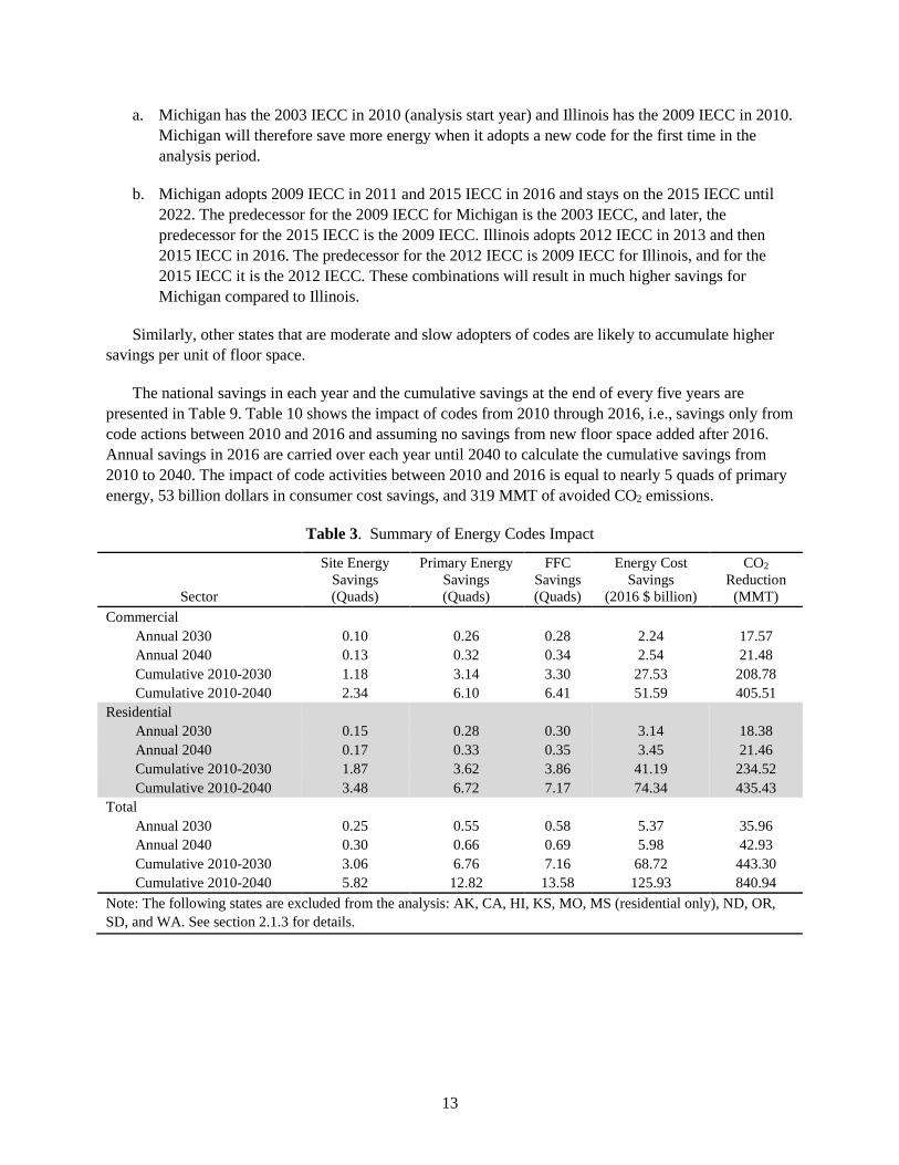
Table 3 summarizes the impact of energy codes aggregated across all the states included in this analysis. Savings are combined from all fuel types (electricity, natural gas, and fuel oil). Annual savings, as defined in section 2.2, are shown for 2030 and 2040, and cumulative savings are shown for 2010-2040. Savings are further broken out into residential and commercial codes. Energy codes save 12.82 quads of primary energy, $126 billion dollars in consumer cost, and reduce 841 million metric tons (MMT) of CO2 on a cumulative basis from 2010-2040. Primary energy savings, FFC savings, and CO2 reductions are split almost equally between commercial and residential buildings, while energy cost savings are roughly 35% higher in residential than commercial. As described in section 2.1.1, the results shown here are substantially lower than the potential savings from energy codes in the entire U.S. because several states were not included.

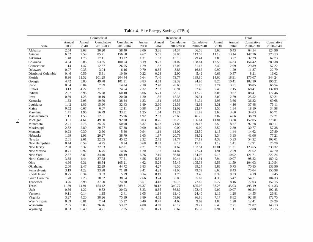
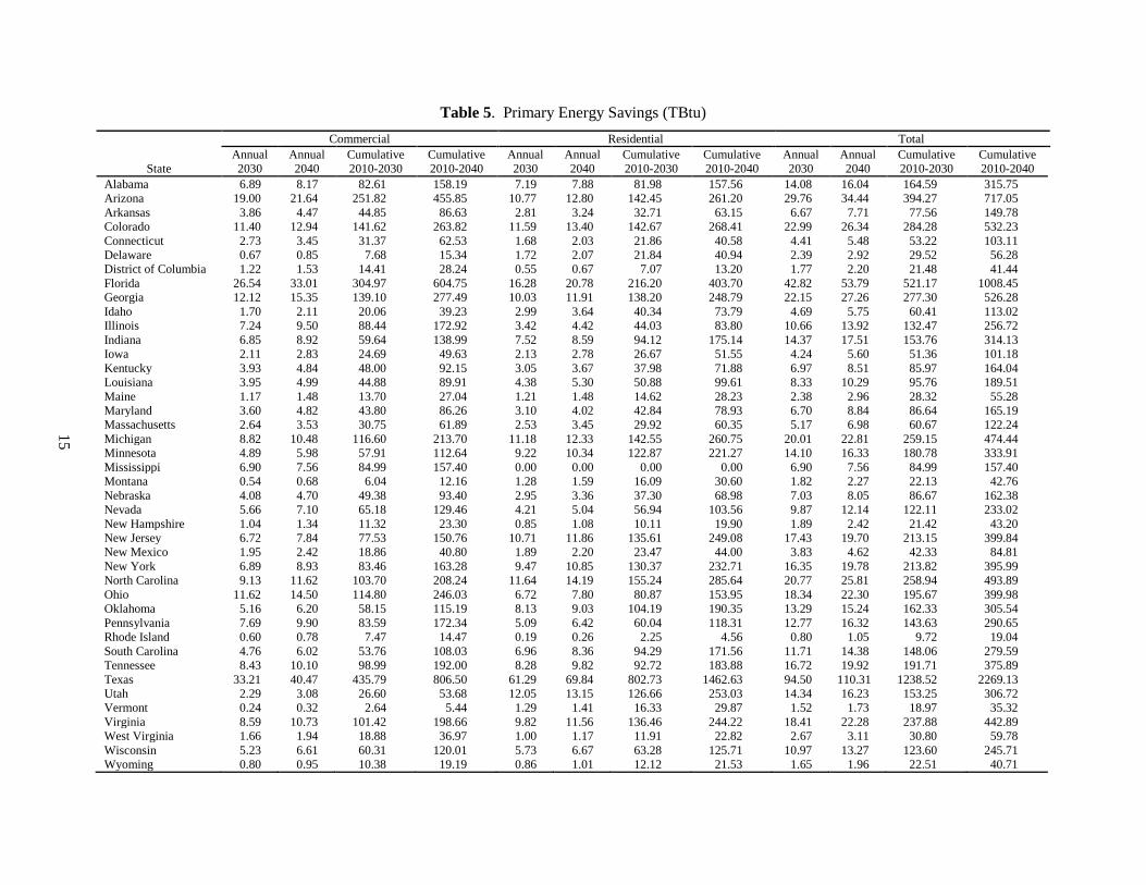
Table 4 through Table 8 show the energy and environmental impacts for each state. Site, primary, and FFC energy savings (TBtu), energy cost savings (billion $ 2016), and CO2 reduction (MMT) are shown in the tables for each state. Commercial and residential savings are shown separately. It can be seen that certain states, such as Texas, Florida, and a few others, have much higher total savings than other states reflecting their relatively higher past and projected new floor space construction. The additive nature of code savings gives rise to significantly higher cumulative savings for these states at the end of the study period.

As explained in section 2.1.2, the rolling baseline approach uses the previous code in place as the baseline. This can give rise to non-intuitive results, such as states which adopt codes in a timely manner saving less energy on a cumulative basis than states which adopt codes at a moderate or slow pace (given equal floor space and same starting code editions). For example, Illinois is a timely adopter of new codes, and Michigan adopts codes at a moderate pace. Comparing the residential cumulative primary energy savings between these states, it can be seen that Illinois saves 111 TBtu whereas Michigan saves 262 TBtu. The higher savings from Michigan result from two main differences:

6 This includes fuel extraction, processing, conveyance to the retail distribution center, and delivery to power plants 7 http://energy.gov/eere/buildings/appliance-and-equipment-standards-program

http://energy.gov/eere/buildings/appliance-and-equipment-standards-program

13

a. Michigan has the 2003 IECC in 2010 (analysis start year) and Illinois has the 2009 IECC in 2010. Michigan will therefore save more energy when it adopts a new code for the first time in the analysis period.

b. Michigan adopts 2009 IECC in 2011 and 2015 IECC in 2016 and stays on the 2015 IECC until 2022. The predecessor for the 2009 IECC for Michigan is the 2003 IECC, and later, the predecessor for the 2015 IECC is the 2009 IECC. Illinois adopts 2012 IECC in 2013 and then 2015 IECC in 2016. The predecessor for the 2012 IECC is 2009 IECC for Illinois, and for the 2015 IECC it is the 2012 IECC. These combinations will result in much higher savings for Michigan compared to Illinois.

Similarly, other states that are moderate and slow adopters of codes are likely to accumulate higher savings per unit of floor space.

The national savings in each year and the cumulative savings at the end of every five years are presented in Table 9. Table 10 shows the impact of codes from 2010 through 2016, i.e., savings only from code actions between 2010 and 2016 and assuming no savings from new floor space added after 2016. Annual savings in 2016 are carried over each year until 2040 to calculate the cumulative savings from 2010 to 2040. The impact of code activities between 2010 and 2016 is equal to nearly 5 quads of primary energy, 53 billion dollars in consumer cost savings, and 319 MMT of avoided CO2 emissions.

Table 3. Summary of Energy Codes Impact

Sector



FFC Savings (Quads)

Energy Cost Savings

(2016 $ billion)

CO2 Reduction

(MMT) Commercial



Total Annual 2030 0.25 0.55 0.58 5.37 35.96



14

Table 4. Site Energy Savings (TBtu)

State

Commercial Residential Total Annual 2030

Annual 2040

Cumulative 2010-2030


Annual 2030

Annual 2040



Annual 2030

Annual 2040



Alabama 2.54 3.08 30.20 58.40 3.06 3.36 34.34 66.56 5.60 6.43 64.54 124.96 Arizona 6.52 7.59 85.71 156.60 4.67 5.55 62.05 113.53 11.19 13.14 147.76 270.13 Arkansas 1.48 1.75 17.11 33.32 1.31 1.52 15.18 29.41 2.80 3.27 32.29 62.73 Colorado 4.34 5.06 53.35 100.54 8.19 9.27 101.07 188.84 12.53 14.33 154.42 289.38 Connecticut 1.14 1.47 12.87 26.05 1.29 1.52 17.02 31.18 2.42 2.99 29.89 57.22 Delaware 0.27 0.35 3.04 6.16 0.70 0.85 8.83 16.62 0.97 1.20 11.87 22.79 District of Columbia 0.46 0.59 5.31 10.60 0.22 0.28 2.90 5.42 0.68 0.87 8.21 16.02 Florida 8.96 11.52 101.29 204.44 5.64 7.40 73.77 139.80 14.60 18.91 175.07 344.24 Georgia 4.42 5.80 49.78 101.31 3.83 4.61 52.32 94.90 8.25 10.41 102.10 196.21 Idaho 0.64 0.84 7.39 14.84 2.10 2.48 28.66 51.70 2.74 3.31 36.05 66.54 Illinois 3.13 4.22 37.51 74.64 2.32 2.92 30.91 57.45 5.45 7.15 68.41 132.09 Indiana 2.97 3.96 25.28 60.18 5.06 5.71 63.12 117.29 8.03 9.67 88.41 177.46 Iowa 0.89 1.23 10.19 20.90 1.20 1.56 15.33 29.31 2.09 2.79 25.52 50.21 Kentucky 1.63 2.05 19.79 38.34 1.33 1.61 16.53 31.34 2.96 3.66 36.32 69.68 Louisiana 1.42 1.86 15.90 32.43 1.89 2.30 21.58 42.68 3.31 4.16 37.48 75.11 Maine 0.52 0.67 6.07 12.11 0.98 1.17 12.02 22.87 1.50 1.84 18.10 34.98 Maryland 1.41 1.96 16.79 33.81 1.25 1.64 17.24 31.89 2.66 3.60 34.03 65.71 Massachusetts 1.11 1.53 12.61 25.96 1.92 2.53 23.68 46.25 3.02 4.06 36.29 72.21 Michigan 3.81 4.61 49.80 92.20 8.03 8.76 102.25 186.61 11.84 13.38 152.05 278.81 Minnesota 2.21 2.76 25.95 50.98 5.37 6.02 71.83 129.13 7.59 8.77 97.78 180.11 Mississippi 2.52 2.80 30.77 57.38 0.00 0.00 0.00 0.00 2.52 2.80 30.77 57.38 Montana 0.23 0.30 2.60 5.30 0.94 1.14 12.02 22.50 1.18 1.44 14.62 27.80 Nebraska 1.69 1.98 20.27 38.70 1.65 1.87 20.79 38.52 3.34 3.85 41.06 77.21 Nevada 2.01 2.61 22.55 45.82 2.32 2.72 31.77 57.19 4.33 5.33 54.32 103.01 New Hampshire 0.44 0.59 4.75 9.94 0.68 0.83 8.17 15.76 1.12 1.41 12.91 25.70 New Jersey 2.80 3.32 32.03 62.81 7.21 7.89 91.62 167.51 10.01 11.21 123.65 230.32 New Mexico 0.71 0.92 6.75 14.96 1.20 1.37 14.87 27.74 1.91 2.29 21.62 42.70 New York 2.87 3.82 34.40 68.19 6.26 7.10 86.81 154.05 9.13 10.92 121.21 222.24 North Carolina 3.38 4.44 37.78 77.21 4.56 5.63 60.44 111.91 7.94 10.07 98.22 189.12 Ohio 4.96 6.31 48.54 105.21 4.62 5.28 55.49 105.33 9.58 11.59 104.03 210.54 Oklahoma 2.00 2.47 22.29 44.72 3.83 4.27 48.56 89.24 5.83 6.73 70.85 133.96 Pennsylvania 3.19 4.22 33.98 71.38 3.41 4.21 41.06 79.59 6.60 8.43 75.04 150.98 Rhode Island 0.25 0.34 3.03 5.99 0.14 0.19 1.76 3.46 0.39 0.53 4.79 9.45 South Carolina 1.70 2.23 18.82 38.64 2.66 3.24 35.89 65.69 4.36 5.47 54.71 104.33 Tennessee 3.26 3.98 37.90 74.30 3.51 4.18 39.13 77.85 6.77 8.16 77.03 152.15 Texas 11.89 14.91 154.42 289.31 26.37 30.12 340.77 625.02 38.25 45.03 495.19 914.33 Utah 0.86 1.22 9.52 20.03 8.23 8.85 86.82 172.42 9.09 10.07 96.34 192.45 Vermont 0.11 0.14 1.15 2.41 1.05 1.14 13.40 24.40 1.16 1.28 14.55 26.81 Virginia 3.27 4.20 38.26 75.89 3.89 4.62 53.92 96.86 7.17 8.82 92.18 172.75 West Virginia 0.69 0.81 7.74 15.27 0.40 0.47 4.68 9.02 1.08 1.28 12.41 24.29 Wisconsin 2.35 3.03 26.76 53.87 4.08 4.69 45.12 89.27 6.43 7.71 71.87 143.13 Wyoming 0.33 0.40 4.21 7.85 0.61 0.71 8.67 15.30 0.94 1.11 12.88 23.15

15

Table 5. Primary Energy Savings (TBtu)

State


Annual 2040



Annual 2030

Annual 2040



Annual 2030

Annual 2040




16

Table 6. FFC Energy Savings (TBtu)

State


Annual 2040



Annual 2030

Annual 2040



Annual 2030

Annual 2040




17

Table 7. Discounted Consumer Cost Savings (Billion $ 2016)

State


Annual 2040



Annual 2030

Annual 2040



Annual 2030

Annual 2040




18

Table 8. Avoided CO2 Emissions (MMT)

State


Annual 2040



Annual 2030

Annual 2040



Annual 2030

Annual 2040




19

Table 9. Annual and 5-Year Cumulative Savings

Year

Site Energy Savings (TBtu)

Primary Energy Savings (TBtu)

FFC Savings (TBtu)

Energy Cost

Savings 2016 $

(billion)

CO2 Reduction

(MMT) 2011 3.53 8.33 8.79 0.09 0.55 2012 10.14 23.94 25.28 0.26 1.57 2013 20.13 47.42 50.07 0.50 3.11 2014 33.78 78.91 83.36 0.85 5.17 2015 54.07 124.88 132.00 1.34 8.19 Cumulative 2011-2015 121.64 283.49 299.50 3.04 18.59 2016 80.36 183.46 194.02 1.98 12.03 2017 109.32 246.21 260.55 2.65 16.13 2018 139.94 312.84 331.18 3.32 20.49 2019 159.80 354.94 375.85 3.72 23.24 2020 179.95 396.98 420.50 4.11 26.02 Cumulative 2016-2020 669.38 1494.43 1582.10 15.79 97.91 2021 200.13 439.12 465.28 4.50 28.84 2022 206.66 454.12 481.13 4.63 29.80 2023 213.32 469.05 496.92 4.76 30.76 2024 220.10 484.04 512.77 4.88 31.74 2025 225.20 495.59 524.97 4.98 32.49 Cumulative 2021-2025 1065.41 2341.93 2481.08 23.75 153.63 2026 230.43 507.26 537.31 5.07 33.25 2027 235.74 518.90 549.61 5.16 34.02 2028 240.15 528.44 559.70 5.23 34.65 2029 244.69 538.23 570.04 5.30 35.30 2030 249.36 548.24 580.63 5.37 35.96 Cumulative 2026-2030 1200.37 2641.08 2797.29 26.14 173.18 2031 253.94 558.18 591.13 5.44 36.62 2032 258.66 568.33 601.85 5.51 37.30 2033 263.56 578.82 612.93 5.57 37.99 2034 268.39 589.18 623.87 5.63 38.67 2035 273.47 600.06 635.35 5.70 39.38 Cumulative 2031-2035 1318.01 2894.57 3065.14 27.85 189.97 2036 278.77 611.45 647.38 5.76 40.12 2037 283.85 622.37 658.90 5.82 40.82 2038 289.09 633.66 670.83 5.87 41.53 2039 294.42 645.18 682.99 5.93 42.26 2040 299.48 656.11 694.53 5.98 42.93 Cumulative 2036-2040 1445.61 3168.77 3354.62 29.36 207.67

20

Table 10. Impact of Codes from 2010-2016

Sector



FFC Savings (Quads)

Energy Cost Savings

2016 $ (billion)

CO2 Reduction

(MMT) Commercial



Total Annual 2016 0.08 0.18 0.19 1.98 12.03


Note: Annual savings in 2016 are assumed to continue accumulating each year until 2040. Savings from new construction beyond 2016 are not included in this table. Also, the following states are excluded from the analysis: AK, CA, HI, KS, MO, MS (residential only), ND, OR, SD, and WA. See section 2.1.3 for details.

21

4.0 References

AIA. 2016. The 2030 Commitment. American Institute of Architects, Washington, D.C. Accessed at: http://www.aia.org/practicing/2030Commitment/

ASHRAE. 2001. ANSI/ASHRAE/IESNA Standard 90.1-2001, Energy Standard for Buildings Except Low-Rise Residential Buildings. ASHRAE, Atlanta, Georgia.

ASHRAE. 2004. ANSI/ASHRAE/IESNA 90.1-2004, Energy Standard for Buildings Except Low-Rise Residential Buildings. ASHRAE, Atlanta, Georgia.



ASHRAE. 2013. ANSI/ASHRAE/IES Standard 90.1-2013. Energy Standard for Buildings Except Low-Rise Residential Buildings. ASHRAE, Atlanta, Georgia.

Bartlett, Rosemarie, M Halverson, J Goins, and P Cole. 2016. Commercial Building Energy Code Compliance Literature Review. PNNL-25218, Pacific Northwest National Laboratory, Richland, Washington. Available at: http://www.pnnl.gov/main/publications/external/technical_reports/PNNL-25218.pdf

BECP. 2016a. Residential Energy Codes Field Study. Building Energy Codes Program, U.S. Department of Energy. Accessed at: www.energycodes.gov/compliance/residential-energy-code-field-study

BECP. 2016b. Status of State Residential Energy Code Adoption as of March 2015. Building Energy Codes Program, U.S. Department of Energy. Accessed at: www.energycodes.gov/adoption/states.

BTO. 2016. BTO Multi-Year Program Plan. Building Technologies Office, U.S. Department of Energy. Accessed at: http://energy.gov/eere/buildings/downloads/multi-year-program-plan Coughlin, K. Projections of Full-Fuel-Cycle Energy and Emissions Metrics. 2013. Lawrence Berkeley National Laboratory: Berkeley, CA. LBNL-6025E. Link: http://eetd.lbl.gov/publications/projections-of-full-fuel-cycle-energy-and-emissions-metrics

BTO. 2015. Solid-State Lighting R&D Plan. Building Technologies Office, U.S. Department of Energy, Washington, D.C. Accessed at: http://www.energy.gov/sites/prod/files/2015/06/f22/ssl_rd-plan_may2015_0.pdf

BTO. 2014a. Windows and Building Envelope Research and Development: Roadmap for Emerging Technologies. Building Technologies Office, U.S. Department of Energy, Washington, D.C. Accessed at: http://energy.gov/sites/prod/files/2014/02/f8/BTO_windows_and_envelope_report_3.pdf

BTO. 2014b. Research and Development Roadmap for Emerging HVAC Technologies. Building Technologies Office, U.S. Department of Energy, Washington, D.C. Accessed at: http://energy.gov/eere/buildings/downloads/research-development-roadmap-emerging-hvac-technologies

http://www.aia.org/practicing/2030Commitment/

http://www.pnnl.gov/main/publications/external/technical_reports/PNNL-25218.pdf

http://www.pnnl.gov/main/publications/external/technical_reports/PNNL-25218.pdf

http://www.energycodes.gov/adoption/states

http://energy.gov/eere/buildings/downloads/multi-year-program-plan

http://eetd.lbl.gov/publications/projections-of-full-fuel-cycle-energy-and-emissions-metrics

http://eetd.lbl.gov/publications/projections-of-full-fuel-cycle-energy-and-emissions-metrics

http://www.energy.gov/sites/prod/files/2015/06/f22/ssl_rd-plan_may2015_0.pdf

http://www.energy.gov/sites/prod/files/2015/06/f22/ssl_rd-plan_may2015_0.pdf

http://energy.gov/sites/prod/files/2014/02/f8/BTO_windows_and_envelope_report_3.pdf

http://energy.gov/eere/buildings/downloads/research-development-roadmap-emerging-hvac-technologies

22

BTO. 2014c. Research and Development Roadmap for Emerging Water Heating Technologies. Building Technologies Office, U.S. Department of Energy, Washington, D.C. Accessed at: http://energy.gov/eere/buildings/downloads/research-development-roadmap-emerging-water-heating-technologies

EIA. 2015. Annual Energy Outlook 2015. U.S. Energy Information Administration. Accessed at http://www.eia.doe.gov/forecasts/aeo/

EIA. 2016a. EIA 826 Electricity Data. Energy Information Administration, Washington, D.C. Last accessed on 07/13/2016 at: https://www.eia.gov/electricity/data/eia826/

EIA. 2016b. Natural gas prices. Energy Information Administration, Washington, D.C. Last accessed on 07/13/2016 at: http://www.eia.gov/naturalgas/data.cfm

EIA. 2016c. State Energy Data System. Energy Information Administration, Washington, D.C. Last accessed on 07/13/2016 at: http://www.eia.gov/state/seds/

EPA. 2016. ENERGY STAR. U.S. Environmental Protection Agency and U.S. Department of Energy, Washington, D.C. Available at: www.energystar.gov

Halverson M. A., R. A. Athalye, M. I. Rosenberg, Y. L. Xie, W. Wang, P. R. Hart, J. Zhang, S. Goel, and V. V. Mendon. 2014. ANSI/ASHRAE/IES Standard 90.1-2013 Determination of Energy Savings: Quantitative Analysis. PNNL-23479, Pacific Northwest National Laboratory, Richland, WA.

ICC. 2003. 2003 International Energy Conservation Code®. International Code Council, Washington D.C.





Livingston, Olga, D Elliott, P Cole, and R Bartlett. 2014. Building Energy Codes Program: National Benefits Assessment, 1992-2040. PNNL-22610, Pacific Northwest National Laboratory, Richland, Washington.

Mendon, Vrushali, Z Taylor, S Rao, and Y Xie. 2015. 2015 IECC: Energy Savings Analysis. PNNL-23977, Pacific Northwest National Laboratory, Richland, Washington.

http://energy.gov/eere/buildings/downloads/research-development-roadmap-emerging-water-heating-technologies

http://energy.gov/eere/buildings/downloads/research-development-roadmap-emerging-water-heating-technologies

http://www.eia.doe.gov/forecasts/aeo/

https://www.eia.gov/electricity/data/eia826/

http://www.eia.gov/naturalgas/data.cfm

http://www.eia.gov/state/seds/

http://www.energystar.gov/

23

Mendon, Vrushali, M Zhao, Z Taylor, and E Poehlman. 2016. 2015 IECC State Cost-effectiveness Analysis–51 state reports. Pacific Northwest National Laboratory, Richland, Washington. Available at: https://www.energycodes.gov/development/residential/iecc_analysis

Lucas, Robert, V Mendon, and S Goel. 2013. Energy Use Savings for a Typical New Residential Dwelling Unit Based on the 2009 and 2012 IECC as Compared to the 2006 IECC. PNNL-88603. Pacific Northwest National Laboratory, Richland, Washington. Available at: https://www.energycodes.gov/sites/default/files/documents/NationalResidentialEnergyAnalysis.pdf

Rosenberg, Michael, R Hart, R Athalye, J Zhang, W Wang, B Liu. 2016. An Approach to Assessing Potential Energy Cost Savings from Increased Energy Code Compliance in Commercial Buildings. Pacific Northwest National Laboratory, Richland, Washington. Available at: http://www.pnnl.gov/main/publications/external/technical_reports/PNNL-24979.pdf.

USGBC. 2016. Leadership in Energy and Environmental Design. U.S. Green Building Council, Washington, D.C. Available at: www.usgbc.org/leed

https://www.energycodes.gov/development/residential/iecc_analysis

https://www.energycodes.gov/sites/default/files/documents/NationalResidentialEnergyAnalysis.pdf

http://www.usgbc.org/leed

Appendix A –

Model Inputs

A.1

Appendix A

Model Inputs

This appendix provides detailed information on the inputs used for adoption, code-to-code savings, floor space, and in the conversion of savings to different energy and environmental units that are used in the codes impact methodology described in section 2.0.

A.1 Adoption

Table A.1 and Table A.2 show the year in which various code editions were adopted by each state, as well as the future rate of adoption (timely, medium slow, or slow) for each state for commercial and residential codes, respectively. The adoption year for code editions up to the 2018 IECC (and 90.1-2016) are shown, but adoption years for future code editions can be calculated by adding the adoption time lag of the state to the year of the published code. In terms of older codes, only 90.1-2001 is shown for commercial and 2003 IECC for residential because all states in the analysis had adopted these codes by 2010—the starting point for the analysis—and thus, there is no need to assess codes older than 90.1-2001 and 2003 IECC.

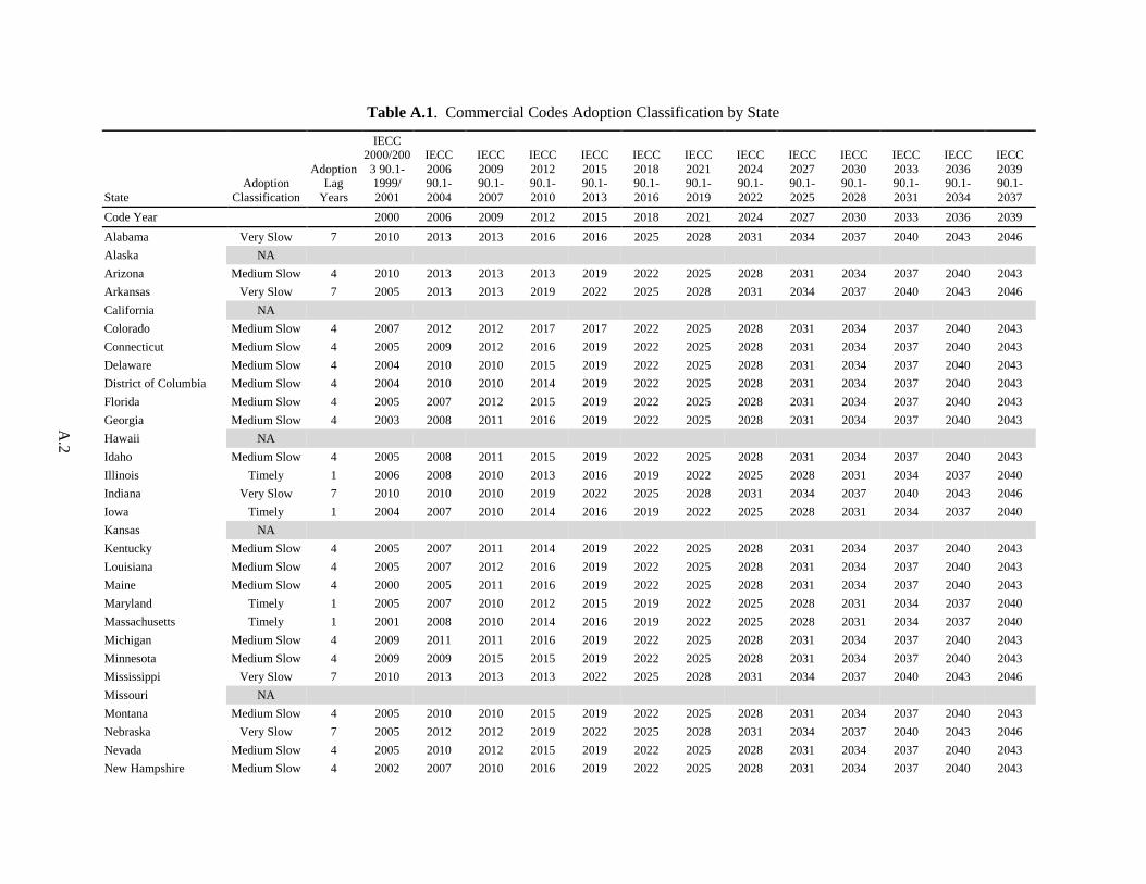
A

.2

Table A.1. Commercial Codes Adoption Classification by State

State Adoption

Classification

Adoption Lag

Years

IECC 2000/2003 90.1-1999/ 2001

IECC 2006 90.1-2004

IECC 2009 90.1-2007

IECC 2012 90.1-2010

IECC 2015 90.1-2013

IECC 2018 90.1-2016

IECC 2021 90.1-2019

IECC 2024 90.1-2022

IECC 2027 90.1-2025

IECC 2030 90.1-2028

IECC 2033 90.1-2031

IECC 2036 90.1-2034

IECC 2039 90.1-2037

Code Year

2000 2006 2009 2012 2015 2018 2021 2024 2027 2030 2033 2036 2039 Alabama Very Slow 7 2010 2013 2013 2016 2016 2025 2028 2031 2034 2037 2040 2043 2046 Alaska NA Arizona Medium Slow 4 2010 2013 2013 2013 2019 2022 2025 2028 2031 2034 2037 2040 2043 Arkansas Very Slow 7 2005 2013 2013 2019 2022 2025 2028 2031 2034 2037 2040 2043 2046 California NA Colorado Medium Slow 4 2007 2012 2012 2017 2017 2022 2025 2028 2031 2034 2037 2040 2043 Connecticut Medium Slow 4 2005 2009 2012 2016 2019 2022 2025 2028 2031 2034 2037 2040 2043 Delaware Medium Slow 4 2004 2010 2010 2015 2019 2022 2025 2028 2031 2034 2037 2040 2043 District of Columbia Medium Slow 4 2004 2010 2010 2014 2019 2022 2025 2028 2031 2034 2037 2040 2043 Florida Medium Slow 4 2005 2007 2012 2015 2019 2022 2025 2028 2031 2034 2037 2040 2043 Georgia Medium Slow 4 2003 2008 2011 2016 2019 2022 2025 2028 2031 2034 2037 2040 2043 Hawaii NA Idaho Medium Slow 4 2005 2008 2011 2015 2019 2022 2025 2028 2031 2034 2037 2040 2043 Illinois Timely 1 2006 2008 2010 2013 2016 2019 2022 2025 2028 2031 2034 2037 2040 Indiana Very Slow 7 2010 2010 2010 2019 2022 2025 2028 2031 2034 2037 2040 2043 2046 Iowa Timely 1 2004 2007 2010 2014 2016 2019 2022 2025 2028 2031 2034 2037 2040 Kansas NA Kentucky Medium Slow 4 2005 2007 2011 2014 2019 2022 2025 2028 2031 2034 2037 2040 2043 Louisiana Medium Slow 4 2005 2007 2012 2016 2019 2022 2025 2028 2031 2034 2037 2040 2043 Maine Medium Slow 4 2000 2005 2011 2016 2019 2022 2025 2028 2031 2034 2037 2040 2043 Maryland Timely 1 2005 2007 2010 2012 2015 2019 2022 2025 2028 2031 2034 2037 2040 Massachusetts Timely 1 2001 2008 2010 2014 2016 2019 2022 2025 2028 2031 2034 2037 2040 Michigan Medium Slow 4 2009 2011 2011 2016 2019 2022 2025 2028 2031 2034 2037 2040 2043 Minnesota Medium Slow 4 2009 2009 2015 2015 2019 2022 2025 2028 2031 2034 2037 2040 2043 Mississippi Very Slow 7 2010 2013 2013 2013 2022 2025 2028 2031 2034 2037 2040 2043 2046 Missouri NA Montana Medium Slow 4 2005 2010 2010 2015 2019 2022 2025 2028 2031 2034 2037 2040 2043 Nebraska Very Slow 7 2005 2012 2012 2019 2022 2025 2028 2031 2034 2037 2040 2043 2046 Nevada Medium Slow 4 2005 2010 2012 2015 2019 2022 2025 2028 2031 2034 2037 2040 2043 New Hampshire Medium Slow 4 2002 2007 2010 2016 2019 2022 2025 2028 2031 2034 2037 2040 2043

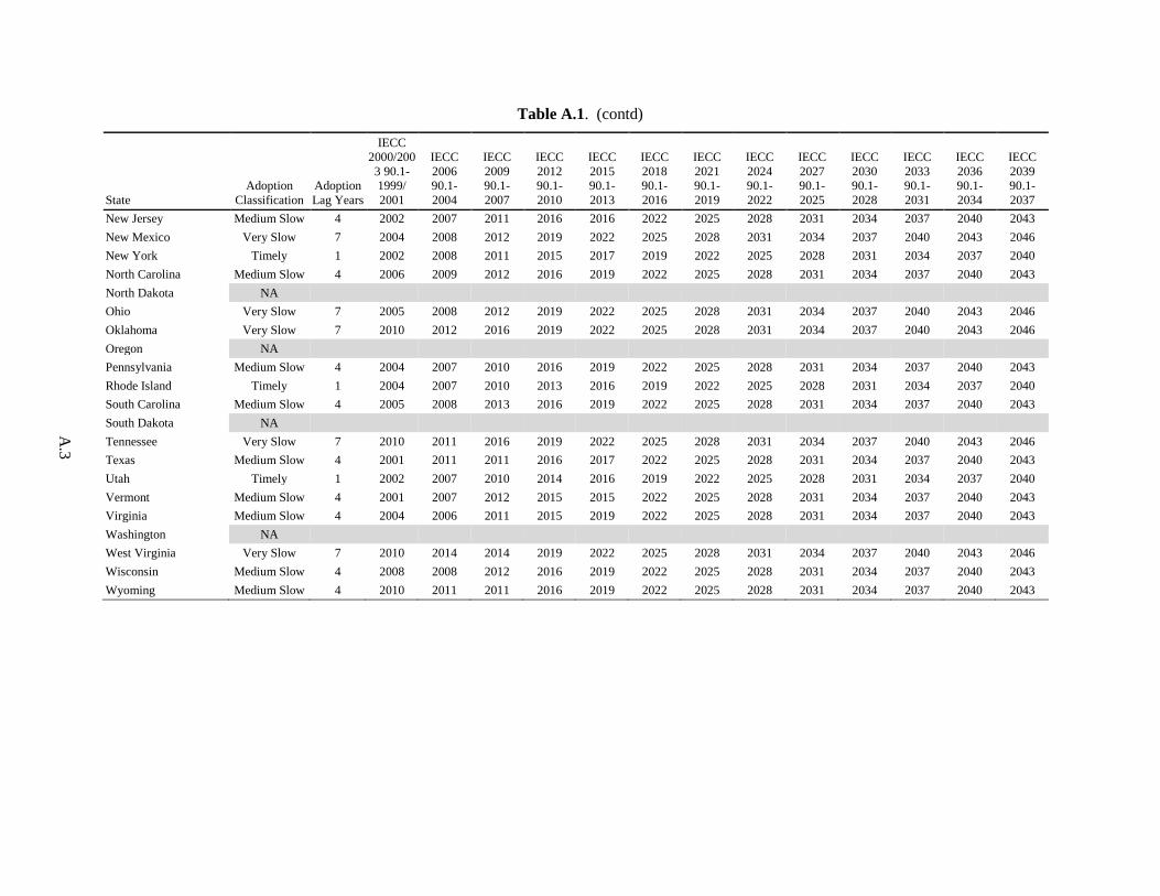
A

.3

Table A.1. (contd)

State Adoption

Classification Adoption Lag Years

IECC 2000/2003 90.1-1999/ 2001

IECC 2006 90.1-2004

IECC 2009 90.1-2007

IECC 2012 90.1-2010

IECC 2015 90.1-2013

IECC 2018 90.1-2016

IECC 2021 90.1-2019

IECC 2024 90.1-2022

IECC 2027 90.1-2025

IECC 2030 90.1-2028

IECC 2033 90.1-2031

IECC 2036 90.1-2034

IECC 2039 90.1-2037

New Jersey Medium Slow 4 2002 2007 2011 2016 2016 2022 2025 2028 2031 2034 2037 2040 2043 New Mexico Very Slow 7 2004 2008 2012 2019 2022 2025 2028 2031 2034 2037 2040 2043 2046 New York Timely 1 2002 2008 2011 2015 2017 2019 2022 2025 2028 2031 2034 2037 2040 North Carolina Medium Slow 4 2006 2009 2012 2016 2019 2022 2025 2028 2031 2034 2037 2040 2043 North Dakota NA Ohio Very Slow 7 2005 2008 2012 2019 2022 2025 2028 2031 2034 2037 2040 2043 2046 Oklahoma Very Slow 7 2010 2012 2016 2019 2022 2025 2028 2031 2034 2037 2040 2043 2046 Oregon NA Pennsylvania Medium Slow 4 2004 2007 2010 2016 2019 2022 2025 2028 2031 2034 2037 2040 2043 Rhode Island Timely 1 2004 2007 2010 2013 2016 2019 2022 2025 2028 2031 2034 2037 2040 South Carolina Medium Slow 4 2005 2008 2013 2016 2019 2022 2025 2028 2031 2034 2037 2040 2043 South Dakota NA Tennessee Very Slow 7 2010 2011 2016 2019 2022 2025 2028 2031 2034 2037 2040 2043 2046 Texas Medium Slow 4 2001 2011 2011 2016 2017 2022 2025 2028 2031 2034 2037 2040 2043 Utah Timely 1 2002 2007 2010 2014 2016 2019 2022 2025 2028 2031 2034 2037 2040 Vermont Medium Slow 4 2001 2007 2012 2015 2015 2022 2025 2028 2031 2034 2037 2040 2043 Virginia Medium Slow 4 2004 2006 2011 2015 2019 2022 2025 2028 2031 2034 2037 2040 2043 Washington NA West Virginia Very Slow 7 2010 2014 2014 2019 2022 2025 2028 2031 2034 2037 2040 2043 2046 Wisconsin Medium Slow 4 2008 2008 2012 2016 2019 2022 2025 2028 2031 2034 2037 2040 2043 Wyoming Medium Slow 4 2010 2011 2011 2016 2019 2022 2025 2028 2031 2034 2037 2040 2043

A

.4

Table A.2. Residential Codes Adoption Classification by State

State Adoption


IECC 2003

IECC 2006

IECC 2009

IECC 2012

IECC 2015

IECC 2018

IECC 2021

IECC 2024

IECC 2027

IECC 2030

IECC 2033

IECC 2036

IECC 2039

Code Year

2003 2006 2009 2012 2015 2018 2021 2024 2027 2030 2033 2036 2039 Alabama Very Slow 7 2010 2013 2013 2016 2016 2025 2028 2031 2034 2037 2040 2043 2046 Alaska NA Arizona Medium Slow 4 2010 2013 2013 2013 2019 2022 2025 2028 2031 2034 2037 2040 2043 Arkansas Very Slow 7 2005 2013 2013 2019 2022 2025 2028 2031 2034 2037 2040 2043 2046 California NA Colorado Medium Slow 4 2007 2012 2012 2017 2017 2022 2025 2028 2031 2034 2037 2040 2043 Connecticut Medium Slow 4 2005 2009 2012 2016 2019 2022 2025 2028 2031 2034 2037 2040 2043 Delaware Medium Slow 4 2004 2010 2010 2015 2019 2022 2025 2028 2031 2034 2037 2040 2043 District of Columbia Medium Slow 4 2004 2010 2010 2014 2019 2022 2025 2028 2031 2034 2037 2040 2043 Florida Medium Slow 4 2005 2007 2012 2015 2019 2022 2025 2028 2031 2034 2037 2040 2043 Georgia Medium Slow 4 2003 2008 2011 2016 2019 2022 2025 2028 2031 2034 2037 2040 2043 Hawaii NA Idaho Medium Slow 4 2005 2008 2011 2015 2019 2022 2025 2028 2031 2034 2037 2040 2043 Illinois Timely 1 2006 2008 2010 2013 2016 2019 2022 2025 2028 2031 2034 2037 2040 Indiana Very Slow 7 2010 2010 2010 2019 2022 2025 2028 2031 2034 2037 2040 2043 2046 Iowa Timely 1 2004 2007 2010 2014 2016 2019 2022 2025 2028 2031 2034 2037 2040 Kansas NA Kentucky Medium Slow 4 2005 2007 2011 2014 2019 2022 2025 2028 2031 2034 2037 2040 2043 Louisiana Very Slow 7 2005 2007 2012 2016 2019 2022 2028 2031 2034 2037 2040 2043 2046 Maine Medium Slow 4 2000 2005 2011 2016 2019 2022 2025 2028 2031 2034 2037 2040 2043 Maryland Timely 1 2005 2007 2010 2012 2015 2019 2022 2025 2028 2031 2034 2037 2040 Massachusetts Timely 1 2001 2008 2010 2014 2016 2019 2022 2025 2028 2031 2034 2037 2040 Michigan Medium Slow 4 2009 2011 2011 2016 2019 2022 2025 2028 2031 2034 2037 2040 2043 Minnesota Medium Slow 4 2009 2009 2015 2015 2019 2022 2025 2028 2031 2034 2037 2040 2043 Mississippi NA Missouri NA Montana Medium Slow 4 2005 2010 2010 2015 2019 2022 2025 2028 2031 2034 2037 2040 2043 Nebraska Very Slow 7 2005 2012 2012 2019 2022 2025 2028 2031 2034 2037 2040 2043 2046 Nevada Medium Slow 4 2005 2010 2012 2015 2019 2022 2025 2028 2031 2034 2037 2040 2043 New Hampshire Medium Slow 4 2002 2007 2010 2016 2019 2022 2025 2028 2031 2034 2037 2040 2043 New Jersey Medium Slow 4 2002 2007 2011 2016 2016 2022 2025 2028 2031 2034 2037 2040 2043 New Mexico Very Slow 7 2004 2008 2012 2019 2022 2025 2028 2031 2034 2037 2040 2043 2046

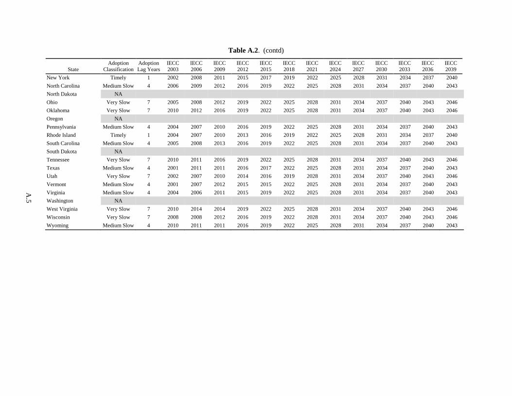
A

.5

Table A.2. (contd)

State Adoption


IECC 2003

IECC 2006

IECC 2009

IECC 2012

IECC 2015

IECC 2018

IECC 2021

IECC 2024

IECC 2027

IECC 2030

IECC 2033

IECC 2036

IECC 2039

New York Timely 1 2002 2008 2011 2015 2017 2019 2022 2025 2028 2031 2034 2037 2040 North Carolina Medium Slow 4 2006 2009 2012 2016 2019 2022 2025 2028 2031 2034 2037 2040 2043 North Dakota NA Ohio Very Slow 7 2005 2008 2012 2019 2022 2025 2028 2031 2034 2037 2040 2043 2046 Oklahoma Very Slow 7 2010 2012 2016 2019 2022 2025 2028 2031 2034 2037 2040 2043 2046 Oregon NA Pennsylvania Medium Slow 4 2004 2007 2010 2016 2019 2022 2025 2028 2031 2034 2037 2040 2043 Rhode Island Timely 1 2004 2007 2010 2013 2016 2019 2022 2025 2028 2031 2034 2037 2040 South Carolina Medium Slow 4 2005 2008 2013 2016 2019 2022 2025 2028 2031 2034 2037 2040 2043 South Dakota NA Tennessee Very Slow 7 2010 2011 2016 2019 2022 2025 2028 2031 2034 2037 2040 2043 2046 Texas Medium Slow 4 2001 2011 2011 2016 2017 2022 2025 2028 2031 2034 2037 2040 2043 Utah Very Slow 7 2002 2007 2010 2014 2016 2019 2028 2031 2034 2037 2040 2043 2046 Vermont Medium Slow 4 2001 2007 2012 2015 2015 2022 2025 2028 2031 2034 2037 2040 2043 Virginia Medium Slow 4 2004 2006 2011 2015 2019 2022 2025 2028 2031 2034 2037 2040 2043 Washington NA West Virginia Very Slow 7 2010 2014 2014 2019 2022 2025 2028 2031 2034 2037 2040 2043 2046 Wisconsin Very Slow 7 2008 2008 2012 2016 2019 2022 2028 2031 2034 2037 2040 2043 2046 Wyoming Medium Slow 4 2010 2011 2011 2016 2019 2022 2025 2028 2031 2034 2037 2040 2043

A.6

A.2 Code-to-Code-Savings

As described in section 2.1.4, code-to-code savings are calculated by using the Determination process. Previous Determinations issued by DOE and the supporting quantitative analysis reports can be found on the BECP website1. These reports include detailed information on EUIs for four commercial and residential code editions: 2004, 2007, 2010, and 2013 editions of 90.1 for commercial, and 2006, 2009, 2012, 2015 editions of the IECC for residential. For codes older than 90.1-2004 and 2006 IECC, the historical EUI index developed by PNNL is used. This index is anchored with a value of 1.0 for the EUI of 90.1-2004 for commercial and 2006 IECC for residential. Going back one edition of codes (because one cycle is all that is needed for this analysis), the EUI index for 90.1-2001 (ASHRAE 2001) is 1.141, and for 2003 IECC (ICC 2003) is 1.012.

Future code EUIs are developed based off the EUI of 90.1-2013 for commercial and 2015 IECC for residential. For future commercial code editions, plug and process loads are not affected. Similarly, the DHW consumption for residential buildings is not affected by code improvements in the future. Energy reduction factors are developed for future code editions as explained in section 2.1.4. These factors are shown in Table A.3 for commercial and Table A.4 for residential. The following steps are taken to develop the energy reduction factors:

1. Start by applying a reduction factor by end-use based on technological progress from BTO’s technology roadmap reports (BTO 2015, 2014, a,b,c).

2. The energy reduction factors for 90.1-2016 are adjusted based on known savings from PNNL’s internal analysis (not published as of August 2016). For residential, no such adjustment is made to 2018 IECC.

3. Finally, the remaining code editions are readjusted based on the changes made to 90.1-2016. No changes are necessary for residential energy reduction factors.

The technological progress is not constant through time. For example, lighting savings in the BTO reports are projected to increase less rapidly up to 2030 and more rapidly beyond 2030. This, and the adjustment to 90.1-2016, is built into the energy reduction factors, and therefore, they are not linear over the period from 2016-2040. The factors vary for different end-uses and depend upon the future potential for improvement for the end-use category. The envelope technology improvements are reflected in the HVAC end-use category. Equipment efficiency improvements are not included in the future projections.

Table A.3. Commercial Future Code Edition Energy Reduction Factors (90.1-2013 = 1.00)

End-Use IECC 2018 90.1-2016

IECC 2021 90.1-2019

IECC 2024 90.1-2022

IECC 2027 90.1-2025

IECC 2030 90.1-2028

IECC 2033 90.1-2031

IECC 2036 90.1-2034

IECC 2039 90.1-2037

Electricity – HVAC 0.90 0.80 0.74 0.68 0.62 0.56 0.50 0.44 Electricity – Lighting 0.92 0.86 0.80 0.72 0.64 0.56 0.48 0.40 NG – HVAC 0.90 0.80 0.74 0.68 0.62 0.56 0.50 0.44 NG – Plug and Process 1.00 1.00 1.00 1.00 1.00 1.00 1.00 1.00 Electricity – Plug and Process

1.00 1.00 1.00 1.00 1.00 1.00 1.00 1.00

1 Determinations on BECP website: https://www.energycodes.gov/determinations


A.7

Table A.4. Residential Future Code Edition Energy Reduction Factors (2015 IECC = 1.00)

End-Use IECC 2018

IECC 2021

IECC 2024

IECC 2027

IECC 2030

IECC 2033

IECC 2036

IECC 2039

Electricity – HVAC 0.95 0.90 0.85 0.80 0.75 0.70 0.65 0.60 Electricity – Lighting 0.96 0.92 0.88 0.80 0.72 0.64 0.56 0.48 Electricity DHW 1.00 1.00 1.00 1.00 1.00 1.00 1.00 1.00 NG – HVAC 0.95 0.90 0.85 0.80 0.75 0.70 0.65 0.60 NG – DHW 1.00 1.00 1.00 1.00 1.00 1.00 1.00 1.00 Oil – HVAC 0.95 0.90 0.85 0.80 0.75 0.70 0.65 0.60 Oil – DHW 1.00 1.00 1.00 1.00 1.00 1.00 1.00 1.00

Table A.5 shows the relative improvement in each future code edition as a percentage reduction in energy consumption of the previous edition given the energy reduction factors established in Table A.3 and Table A.4. These overall code-to-code savings are calculated by first weighting the state-level results up to the national level and then comparing the national weighted EUIs. Future code editions have a smaller impact on both the annual and cumulative savings calculated in this analysis because the savings have less time to add up.

Table A.5. Future Code Edition Savings Commercial Residential

Code Edition

% Savings Compared to

Previous Code Code

Edition

% Savings Compared to

Previous Code 90.1-2016 5 2018 IECC 4 90.1-2019 5 2021 IECC 4 90.1-2022 4 2024 IECC 4 90.1-2025 4 2027 IECC 4 90.1-2028 5 2030 IECC 5 90.1-2031 5 2033 IECC 5 90.1-2034 5 2026 IECC 5 90.1-2037 5 2039 IECC 5

A.3 Floor Space

As described in section 2.1.6, new floor space added from 1992 to 2040 calculated in a previous analysis (Livingston et al. 2014) is used in this analysis. The previous analysis used data from AEO 2012. Since the publication of the previous analysis, new data has become available from EIA and this data is used to update new floor space added each year. This and other updates are described in detail here.

Commercial floor space updates. For the commercial forecast, the underlying source of floor space forecasts is updated from AEO 2012 to AEO 2015 (EIA 2015). Data from AEO 2015 is also used to update scaling factors that are used to realistically meld the historical floor space data with the AEO data. Specifically, scaling factors that were forecasted for the years 2011 through 2015 in the previous analysis are adjusted in order to provide a more realistic transition from the depressed construction levels of 2010. Factors from the previous analysis and the ones calculated for the current analysis are shown in Table A.6.

A.8

Table A.6. Commercial Floor Space Scaling Factors 2011-2014

Year

Scaling Factors from Livingston et al.

2014 New Scaling

Factors 2011 0.6306 0.6328 2012 0.6203 0.6172 2013 0.7544 0.7412 2014 0.9011 0.8320

Residential floor space updates. Residential floor space estimates are based on households, and again the underlying AEO data from 2012 is updated using newer data from AEO 2015. Other changes are made to the residential household estimates and are described below.

1. In the prior analysis, Census Bureau residential building permit data, for the years 1991 through 2012, were used to develop a time-series of historical floor space estimates. This time series is extended through 2014 in the current analysis.

2. The fraction of multi-family units classified as low-rise is estimated using 2005-2014 Census Bureau building permit data in this analysis, whereas in the prior analysis, data from the years 2003-2012 were utilized. This multi-family fraction is applied to AEO-derived multi-family household data to extract an estimate of low-rise multi-family households added each year.

3. As in the previous analysis, annual residential stock survival factors from EIA’s National Energy Modeling System (NEMS) residential documentation are applied to the stock to derive a forecast of additions to residential stock. However, the factors changed slightly as shown in Table A.7.

Table A.7. Residential Stock Survival Factors

Type of Building Stock

Stock Survival Factors from

Livingston et al. 2014

New Stock Survival Factor

Single-family 0.996 0.997 Multi-family 0.999 0.995 Mobile home 0.976 0.966

4. A correction to the size of the prototype single-family home is applied, reducing the size to 2,376 square feet from the prior 2,400 square feet. This updated value is obtained from the Methodology for Evaluating Cost-Effectiveness of Residential Energy Code Changes (Taylor et al. 2015).

5. Regarding the integration of historical and projected data (discussed in section 4.2.3 of the previous report), the Census data are at the state level, and provide data for the years 1992 through 2014. The AEO data are at the Census Division level, and include data for the years 2009 through 2040. These two data series, which reasonably closely match for overlapping years, are melded to provide a Census Division-level series. In order to generate state-level time-series data through 2040, growth rates inferred from the melded Census Division-level time series are applied to the 2014 state-level Census data. An implicit assumption is that state shares within each Census Division remain constant at 2014 levels.

A.9

A.4 Savings Conversions

Energy Prices. Energy prices are used for computing consumer cost savings by applying prices to the site energy savings. Prices for electricity, natural gas, and fuel oil are derived from EIA databases such as EIA 826, Natural Gas Navigator, and State Energy Data System (EIA 2016a,b,c). Once energy prices are obtained from these databases, the actual forecast indices calculated from AEO price data are applied to each fuel price to derive the future stream of annual prices for each fuel. Prices are expressed in real dollars. Subsequently, the energy savings in each year are used in conjunction with relevant fuel prices to estimate the financial benefits accrued with time. A discounted cash flow framework with a real discount rate of 5% is then used to discount the future stream of benefits back to year 2016 monetary values. A discount rate of 5% is chosen as an average between 3% and 7%, which are the boundary values used in various federal rulemaking analyses at PNNL.

Environmental Conversion Factors. Coughlin describes a method and provides a generic framework to calculate utility sector impacts (Coughlin 2013). This framework is used in the analysis. Conversion factors are obtained from NEMS through the National Impact Analysis Plus (NIAplus) model. This module consists of annual time series of different factors (MMBtu/kWh, or kg emissions/kWh) that allow conversion of site energy savings to different energy and environmental units.

Appendix B –

Site Energy Savings By Fuel Type

B

.1

Table B.1. Electricity Site Energy Savings by State (TBtu)

State


Annual 2040



Annual 2030

Annual 2040



Annual 2030

Annual 2040




B

.2

Table B.2. Natural Gas Site Energy Savings by State (TBtu)

State


Annual 2040



Annual 2030

Annual 2040



Annual 2030

Annual 2040




B

.3

Table B.3. Fuel Oil Site Energy Savings by State (TBtu)

State


Annual 2040



Annual 2030

Annual 2040



Annual 2030

Annual 2040



Alabama 0.00 0.00 0.00 0.00 0.00 0.00 0.00 0.00 0.00 0.00 0.00 0.00 Arizona 0.00 0.00 0.00 0.00 0.00 0.00 0.06 0.11 0.00 0.00 0.06 0.11 Arkansas 0.00 0.00 0.00 0.00 0.00 0.00 0.00 0.00 0.00 0.00 0.00 0.00 Colorado 0.00 0.00 0.00 0.00 0.02 0.02 0.20 0.38 0.02 0.02 0.20 0.38 Connecticut 0.00 0.00 0.00 0.00 0.39 0.45 5.25 9.50 0.39 0.45 5.25 9.50 Delaware 0.00 0.00 0.00 0.00 0.00 0.00 0.01 0.03 0.00 0.00 0.01 0.03 District of Columbia 0.00 0.00 0.00 0.00 0.00 0.00 0.00 0.01 0.00 0.00 0.00 0.01 Florida 0.00 0.00 0.00 0.00 0.00 0.00 0.04 0.07 0.00 0.00 0.04 0.07 Georgia 0.00 0.00 0.00 0.00 0.00 0.01 0.06 0.11 0.00 0.01 0.06 0.11 Idaho 0.00 0.00 0.00 0.00 0.00 0.00 0.06 0.10 0.00 0.00 0.06 0.10 Illinois 0.00 0.00 0.00 0.00 0.01 0.01 0.15 0.27 0.01 0.01 0.15 0.27 Indiana 0.00 0.00 0.00 0.00 0.02 0.03 0.30 0.56 0.02 0.03 0.30 0.56 Iowa 0.00 0.00 0.00 0.00 0.00 0.01 0.06 0.11 0.00 0.01 0.06 0.11 Kentucky 0.00 0.00 0.00 0.00 0.00 0.00 0.00 0.00 0.00 0.00 0.00 0.00 Louisiana 0.00 0.00 0.00 0.00 0.00 0.00 0.00 0.00 0.00 0.00 0.00 0.00 Maine 0.00 0.00 0.00 0.00 0.31 0.36 3.85 7.23 0.31 0.36 3.85 7.23 Maryland 0.00 0.00 0.00 0.00 0.00 0.00 0.03 0.05 0.00 0.00 0.03 0.05 Massachusetts 0.00 0.00 0.00 0.00 0.58 0.73 7.40 14.04 0.58 0.73 7.40 14.04 Michigan 0.00 0.00 0.00 0.00 0.04 0.05 0.54 0.98 0.04 0.05 0.54 0.98 Minnesota 0.00 0.00 0.00 0.00 0.02 0.02 0.28 0.51 0.02 0.02 0.28 0.51 Mississippi 0.00 0.00 0.00 0.00 0.00 0.00 0.00 0.00 0.00 0.00 0.00 0.00 Montana 0.00 0.00 0.00 0.00 0.00 0.00 0.02 0.05 0.00 0.00 0.02 0.05 Nebraska 0.00 0.00 0.00 0.00 0.01 0.01 0.08 0.16 0.01 0.01 0.08 0.16 Nevada 0.00 0.00 0.00 0.00 0.00 0.00 0.05 0.09 0.00 0.00 0.05 0.09 New Hampshire 0.00 0.00 0.00 0.00 0.21 0.25 2.58 4.89 0.21 0.25 2.58 4.89 New Jersey 0.00 0.00 0.00 0.00 0.37 0.40 4.69 8.53 0.37 0.40 4.69 8.53 New Mexico 0.00 0.00 0.00 0.00 0.00 0.00 0.03 0.05 0.00 0.00 0.03 0.05 New York 0.00 0.00 0.00 0.00 0.32 0.35 4.44 7.81 0.32 0.35 4.44 7.81 North Carolina 0.00 0.00 0.00 0.00 0.01 0.01 0.08 0.14 0.01 0.01 0.08 0.14 Ohio 0.00 0.00 0.00 0.00 0.02 0.03 0.28 0.52 0.02 0.03 0.28 0.52 Oklahoma 0.00 0.00 0.00 0.00 0.00 0.00 0.00 0.00 0.00 0.00 0.00 0.00 Pennsylvania 0.00 0.00 0.00 0.00 0.17 0.20 2.06 3.90 0.17 0.20 2.06 3.90 Rhode Island 0.00 0.00 0.00 0.00 0.04 0.05 0.55 1.04 0.04 0.05 0.55 1.04 South Carolina 0.00 0.00 0.00 0.00 0.00 0.00 0.05 0.08 0.00 0.00 0.05 0.08 Tennessee 0.00 0.00 0.00 0.00 0.00 0.00 0.00 0.00 0.00 0.00 0.00 0.00 Texas 0.00 0.00 0.00 0.00 0.00 0.00 0.00 0.00 0.00 0.00 0.00 0.00 Utah 0.00 0.00 0.00 0.00 0.02 0.02 0.17 0.33 0.02 0.02 0.17 0.33 Vermont 0.00 0.00 0.00 0.00 0.33 0.36 4.26 7.73 0.33 0.36 4.26 7.73 Virginia 0.00 0.00 0.00 0.00 0.01 0.01 0.08 0.14 0.01 0.01 0.08 0.14 West Virginia 0.00 0.00 0.00 0.00 0.00 0.00 0.01 0.01 0.00 0.00 0.01 0.01 Wisconsin 0.00 0.00 0.00 0.00 0.02 0.02 0.23 0.44 0.02 0.02 0.23 0.44 Wyoming 0.00 0.00 0.00 0.00 0.00 0.00 0.02 0.03 0.00 0.00 0.02 0.03 Note: Fuel oil is not represented in the commercial building models.

Appendix C –

Maximum Potential Savings

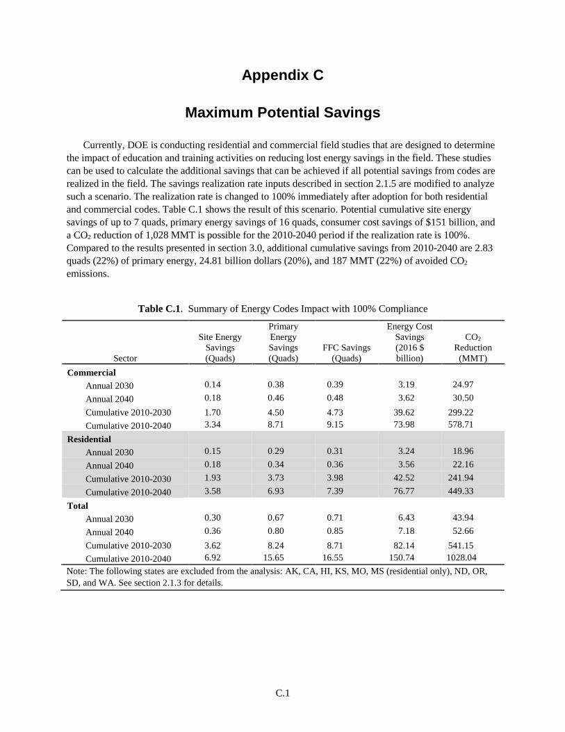
C.1

Appendix C

Maximum Potential Savings

Currently, DOE is conducting residential and commercial field studies that are designed to determine the impact of education and training activities on reducing lost energy savings in the field. These studies can be used to calculate the additional savings that can be achieved if all potential savings from codes are realized in the field. The savings realization rate inputs described in section 2.1.5 are modified to analyze such a scenario. The realization rate is changed to 100% immediately after adoption for both residential and commercial codes. Table C.1 shows the result of this scenario. Potential cumulative site energy savings of up to 7 quads, primary energy savings of 16 quads, consumer cost savings of $151 billion, and a CO2 reduction of 1,028 MMT is possible for the 2010-2040 period if the realization rate is 100%. Compared to the results presented in section 3.0, additional cumulative savings from 2010-2040 are 2.83 quads (22%) of primary energy, 24.81 billion dollars (20%), and 187 MMT (22%) of avoided CO2

emissions.

Table C.1. Summary of Energy Codes Impact with 100% Compliance

Sector



FFC Savings (Quads)

Energy Cost Savings (2016 $ billion)

CO2 Reduction

(MMT) Commercial



Total Annual 2030 0.30 0.67 0.71 6.43 43.94 Annual 2040 0.36 0.80 0.85 7.18 52.66 Cumulative 2010-2030 3.62 8.24 8.71 82.14 541.15 Cumulative 2010-2040 6.92 15.65 16.55 150.74 1028.04


Impacts of Model Building Energy Codes

Documents

Transcript of Impacts of Model Building Energy Codes