1

Impact of macroeconomic news on metal futures1 John Eldera, Hong Miaoa, Sanjay Ramchandera,* a Department of Finance and Real Estate, Colorado State University, USA.

This version: August 1, 2011

______________________________________________________________________________

Abstract

This paper uses intra-day data for the period 2002 through 2008 to examine the intensity, direction, and speed of impact of U.S. macroeconomic news announcements on the return, volatility and trading volume of three important commodities – gold, silver and copper futures. We find that the response of metal futures to economic news surprises is both swift and significant, with the 8:30 am set of announcements – in particular, nonfarm payrolls and durable goods orders – having the largest impact. Furthermore, announcements that reflect an unexpected improvement in the economy tend to have a negative impact on gold and silver prices; however, they tend to have a positive effect on copper prices. In comparison, realized volatility and volume for all three metals are positively influenced by economic news. There is also evidence that several news announcements exert an asymmetric impact on market activity variables. Finally, we are able to construct a profitable trading strategy using information from the news surprises.

JEL classification: G14 Keywords: Macroeconomic news; Metal futures _____________________________________________________________________________ * Corresponding author. Tel.: +1 970 491 6681; fax: +1 970 491 6196. E-mail addresses: john.elder@business.colostate.edu (J. Elder), hong.miao@business.colostate.edu (H. Miao), sanjay.ramchander@business.colostate.edu (S. Ramchander) 1 This version includes a new section (section 6: A simple trading rule). The original paper without the new section has been accepted for publication at the Journal of Banking and Finance.

2

1. Introduction

The relationship between information arrival and asset price movements is of central importance

to price formation and price discovery in financial markets, and is a topic that has been

extensively investigated in the literature. For instance, the mixture of distributions model relies

on “news” to explain movements in asset returns (see Tauchen and Pitts, 1983). Among the

various sources of information the role of public information is frequently examined because

they are easily identifiable, and also carry implications for the canonical model of weakly

efficient markets which posits that security prices reflect all available information. Chen, Roll,

and Ross (1986) highlight the importance of macroeconomic factors such as industrial

production and measures of unanticipated inflation on stock returns. In a related study, Flannery

and Protopapadakis (2002) relate equity returns to macroeconomic variables. More recently,

research attention has shifted to an examination of intra-day data that provides additional insights

into the market microstructure behavior relating to trading and pricing variables. As a case in

point, Adams, McQueen, and Wood (2004) show that unanticipated inflationary news has

distinguishable effects on intra-day equity returns, and that most of this information is

incorporated within minutes of the news release.

This paper explores the price formation process and trading volume activity in the metals

futures market around the release of new macroeconomic information. Four important questions

are addressed. First, what is the impact of macroeconomic news on the return, realized volatility

and volume of gold, silver and copper futures? Second, does the release of macroeconomic news

affect the three metals in different ways? Third, how long does it take for the impact of

macroeconomic news shocks to be fully absorbed by the market? Finally, does the metals market

respond asymmetrically to the release of unexpected macroeconomic news?

3

The answers to these questions are important for several reasons. First, our analysis is based

on high-frequency intra-day data, which allows us to detect patterns of market reaction that may

not be easily discerned in lower frequency daily data. In this regard, it is important to point out

that the empirical literature using daily data finds only mixed or relatively weak evidence of the

link between macroeconomic announcements and commodity prices (see Roache and Rossi,

2010; Hess, Huang and Niessen, 2008), thus lending support to the argument that, unlike other

assets, commodity prices are predetermined with respect to U.S. macroeconomic aggregates such

as real output, consumption and investment variables (Kilian and Vega, 2010). Therefore, an

investigation of how an important class of commodities, specifically metals, responds to

macroeconomic news at intra-day frequencies provides a meaningful contrast with existing

studies. Based on Andersen’s (1996) argument that different types of news may have different

stochastic arrival processes and therefore convey varying impacts on pricing behavior, we

evaluate the impact of 19 different types of macroeconomic news. These announcements are

sorted by the time of each news release, with the aim of identifying those announcement times

that have the largest impact on the metals market. Furthermore, taking into account evidence

from related asset markets such as equities (Koutmos and Booth, 1995), we also examine

whether or not metal futures respond asymmetrically to economic news. We contend that a study

of how metal futures prices react to positive versus negative economic surprises would be

informative not only in terms of market efficiency and information processing, but may also

provide an explanation as to why previous studies that do not account for potential asymmetries

may have been unsuccessful in documenting a significant relationship between economic news

and commodity prices.

4

Second, compared to financial assets, there is a relative paucity of studies that examine the

role of information in the metal futures markets. This is especially noteworthy considering that in

recent years there has been a steady increase in the amount of investor attention given to these

markets. In general, the popularity of commodities, and in particular metals, stems from the

belief that these assets act as a hedge against inflation, offer valuable diversification

opportunities to investors, serve as a monetary medium during times of market uncertainty, and

have a wide range of manufacturing and industrial applications. It is therefore not entirely

surprising that these products are one of the most heavily traded in organized futures exchanges.

Finally, our study is comprehensive in scope in that it evaluates the responsiveness of several

market activity variables including return, volatility and trading volume. We construct a realized

volatility measure that accounts for intra-day price information within each particular time

interval.

Therefore, to summarize, our sample period, research design, and empirical methods allow us

to investigate more fully the high-frequency dynamics of three important commodities. The

remainder of the paper is organized as follows. In the next two sections we provide a literature

review and discuss theoretical considerations, respectively. Section 4 explains the data sources,

summary statistics and cleaning procedures. Section 5 provides a brief description of the research

design and empirical methods, and discusses the results. Section 6 concludes the paper.

2. Literature review

A survey of the literature in the metals commodities markets reveals three major research

streams: (a) characterization of the distributional properties of metal prices (Khalifa, Miao and

Ramchander, 2011); (b) identification of dynamic relationships between futures and spot prices

of various metals (Kocagil, 1997); and (c) examination of metals as a hedge against inflation,

5

currency rate risk, and market uncertainty (Baur and Lucey, 2010). Our study on how metal

futures market responds to macroeconomic news adds a new dimension to the literature and

carries implications for market efficiency, risk premia, and the pricing and trade behavior of

gold, copper and silver.

Although there is a vast amount of literature that documents the effects of macroeconomic

news on stocks (e.g., Boyd, Hu and Jagannathan, 2005), bonds (e.g., Simpson and Ramchander,

2004; Nowak et al., 2011) and currencies (e.g., Simpson, Ramchander and Chaudhry, 2005;

Chen and Gau, 2010), the corresponding literature on the reaction of metal prices to economic

announcements is relatively scarce. Some notable exceptions exist. Using daily data, in a broader

examination of 12 different commodities including gold, silver and copper, Roache and Rossi

(2010) find that daily prices are relatively insensitive to macroeconomic news. Hess, Huang and

Niessen (2008) provide a state-dependent interpretation of macroeconomic news by showing that

daily commodity prices are responsive only during recessionary periods, but not during periods

of economic growth.

To our knowledge there are only two studies that use intra-day data to examine gold and/or

silver prices. Christie-David, Chaudhry and Koch (2000) use intra-day 15-minute transaction

prices between 1992 and 1995 to show that the impact of economic surprises on the return

variance of gold and silver futures prices is less pronounced compared to interest rate futures.

Cai, Cheung and Wong (2001) provide a detailed characterization of return volatility in gold

futures using 5-minute returns between 1994 and 1997. They find that the impact of

macroeconomic announcements is much smaller on gold compared to the impact on Treasury

bond or currency markets, and only four announcements – jobs report, inflation, GDP and

personal income – carry statistically significant effects on gold volatility.

6

Our study differs from both Christie-David et al. (2000) and Cai et al. (2001) in several

regards. First, we use a longer and more recent time frame (2002 through 2008) for the analysis,

a period during which metal prices experienced a dramatic increase in price and trading activity.

For instance, the futures price of gold increased more than threefold during this period (from

about $278 per troy ounce in 2002 to about $1,003 in 2008). There was also a corresponding rise

in aggregate trading volume from about 6.8 million contracts in 2001 to more than 38 million in

2008. 2 Second, our study is more comprehensive in scope since we consider the impact of

economic news on three important market activity variables – i.e., returns, volatility and trading

volume. Third, we differentiate our work from prior studies by constructing a realized volatility

measure that has been shown to provide consistent estimates of integrated volatility in the

underlying price process (see Barndorff-Nielsen and Shepard, 2002).3 A final point of distinction

is that our study allows for the possibility of return, realized volatility and volume measures to

respond asymmetrically to macroeconomic news announcements, and examines the persistence

of economic shocks in the metals futures market.

3. Theoretical considerations

Physical commodities are different from most financial assets in that they are continuously

produced and consumed. The fact that they can be stored implies that production need not be

consumed at once. Therefore, mismatches between production and consumption levels can lead

to either accumulation or depletion of inventory resulting in price changes. The theory of storage

2 The price movement in the copper market is even more dramatic. Its price was about $0.66 per pound at the beginning of 2002 and reached a peak in July 2008 when it closed at about $4.04 per pound; only to drop precipitously to about $1.26 at the end of 2008. The aggregated volume in copper futures increased from 2.8 million contracts in 2001 to 4.56 million contracts in 2008. Silver also seem to have followed a similar meteoric rise. It was about $4.53 per troy ounce at the beginning of 2002 and closed at its peak at $20.92 in March 2008. The aggregate volume of silver futures increased from 2.58 million in 2001 to 8.8 million in 2008. 3 Note that, however, the presence of microstructure noise may bias realized volatility estimates. We account for such potential bias using alternative estimators, as discussed in the ‘research design’ section of the study.

7

(see Brennan, 1958) highlights the role of the interest costs of storing the commodity as an

important determinant of commodity price changes. In this framework, an unexpected increase in

interest rates reduces the demand for inventories (since it raises storage costs) and puts

downward pressure on commodity prices.

Unfortunately, given that aggregate inventories are usually not observable and inventory

estimates are subject to potential misrepresentation, one may have to explain observed price

changes in the context of information arrival. It is in this context that an examination of

macroeconomic news, which reveals new information about future economic conditions,

becomes pertinent in explaining commodity price movements. However, it must be noted that

although news releases are expected to affect commodity prices by altering market beliefs about

future economic conditions, the direction of the impact is indeterminate a priori. For instance,

announcements that cause market participants to revise their expectations of inflation upwards

may lead investors to rebalance their portfolios by shifting out of money and into physical assets

like commodities. This is likely to result in a positive price change. On the other hand, based on

the policy anticipation hypothesis, if market participants anticipate a tighter monetary policy

response to curb higher inflation, this may cause real interest rates to rise, and along with slower

expected economic growth, drive down commodity prices. In sum, the response of commodity

price changes to macroeconomic news is an empirical issue since the price response function is

an amalgam of inflation expectations and expected monetary policy response.

Predicting the price response can be further complicated by the fact that there is a wide

degree of variation among individual commodity types. This is illustrated by Erb and Harvey

(2006) who find a low degree of correlation between different commodity futures products. In

the case of metals, it would be reasonable to expect that the price response of precious metals

8

(gold and silver) which are often seen as an alternative investment vehicle is different from

industrial metals such as copper which is viewed a primary input in manufacturing. Therefore, it

is possible that a surprise improvement in economic growth may cause gold and silver prices to

drop because of portfolio rebalancing effects, but result in higher copper prices due to greater

industrial demand.

The pattern of the response of trading volume to anticipated announcements may also

take different forms. Theoretical trading models such as Glosten and Milgrom (1985) endow

informed traders with private information about impending announcements. Prior to anticipated

announcements, these models imply that liquidity declines, as market makers seek to protect

themselves from trading with informed traders, while volume may increase as long as the

benefits of informed trading exceed the costs of trading. In these models, the public

announcement ameliorates the advantage of the informed traders, and volume may be either low

or high, depending on whether there is pent up demand from uninformed traders.

In models such as that described by Kim and Verrecchia (1994), the acquisition of private

information prior to the announcement is endogenous, and depends on the cost of acquiring

private information as well as the expected quality of the announcement. They find that volume

after the announcement is directly related to price volatility (measured as the absolute value of

the price change), with an increase in the quality of the announcement tending to strengthen the

reaction of volume. There is no reason for these characterizations to be mutually exclusive, so an

empirical study can offer evidence on which effect tends to dominate.

Finally, in comparison to returns and volume, our expected response of volatility is

somewhat more predictable. Ross (1989) argues that in an arbitrage free economy return

volatility should be related to information arrival or variation in information frequencies. This

9

argument is supported by Pasquariello and Vega (2007) who find that, ceteris paribus, price

volatility increases in the presence of public information signals. Our research attempts to

disentangle these various effects.

4. Data characteristics

4.1. Futures prices and macroeconomic announcements data

Our data on metals prices consists of intra-day, tick-by-tick, futures transaction prices for gold,

silver and copper for the period January 2002 through December 2008. The data for trading

volume is available only for 2007 and 2008. The futures data is obtained from the Futures

Industry Institute.

Gold, silver and copper metal futures trade on the Chicago Mercantile Exchange (CME),

which provides both open outcry (pit) and electronic (Globex) trading. Open outcry trading

occurs Monday through Friday during the following hours (Eastern Standard Time): 8:20 am –

1:30 pm for gold, 8:25 am – 1:25 pm for silver, and 8:10 am – 1:00 pm for copper. Trading is

also offered simultaneously on the Globex electronic trading platform Sunday through Friday

from 6:00 pm – 5:15 pm. The raw tick-by-tick futures price data specifies the time, to the nearest

second, and the price of the futures transaction. We construct a continuous price series from front

month contract, rolling over to the next contract when the daily tick volume of the first back-

month contract exceeds the daily tick volume of the current front month contract. This procedure

avoids stale prices from the front-month contract that typically occur in the four weeks prior to

expiration. The futures prices are then sampled at 1-minute discrete intervals, yielding about

500,000 price observations for each metal. The 1-minute observations are then used to construct

5-minute return and volatility measures.

10

Table 1 reports summary statistics for the daily return series for gold, silver and copper. Gold

has a daily mean return of 0.065% and standard deviation 1.23%. Copper and silver have daily

mean returns of 0.0426% and 0.0511% respectively, and both have a daily standard deviation of

about 2%. The distribution of the return series for each metal exhibits negative skewness and

excess kurtosis, and for each series the Jarque-Bera test rejects the null hypothesis of normality.

Our data on macroeconomic news releases consists of 19 different announcements and is

obtained from Bloomberg. For each announcement, we collect both the realized value and the

consensus (median) forecast as reported in Bloomberg. Each announcement is released monthly

on pre-arranged schedule and disseminated immediately on newswires and other data providers.

In order to make meaningful comparison of the estimated news impact across the three asset

classes and different news releases, we “standardize” the news measures. Specifically, the

unanticipated component, or surprise, in each announcement is computed as the difference

between the actual (or realized) value and the consensus forecast, normalized by its standard

deviation. Let 𝐴𝑖,𝑡 denote the realized value of an announcement of type 𝑖 at time t, and 𝐸𝑖,𝑡

denote the consensus forecast. The standardized surprise element of the announcement is defined

as:

𝑆𝐴𝑖,𝑡 = 𝐴𝑖,𝑡−𝐸𝑖,𝑡𝜎𝑖

, (1)

where 𝜎𝑖 is the sample standard deviation of the surprise component of the type 𝑖 announcement,

𝐴𝑖,𝑡 − 𝐸𝑖,𝑡. Because 𝜎𝑖 is constant for each announcement, the standardization procedure should

not affect the statistical significance of the estimated response coefficients and fit of the

regression model.

We also calibrate each surprise announcement so that a positive value represents stronger-

than-expected economic growth, and a negative value represents weaker-than-expected

11

economic growth. Therefore, we switch the sign for the unemployment rate surprise so that

positive surprise represents an unemployment rate that is lower than expected.

We classify the 19 macroeconomic announcements into three categories depending on the

time of each announcement. There are 11 announcements at 8:30 am, 2 announcements at 9:15

am, and 7 announcements at 10:00 am.4 Table 2 reports the different types of macroeconomic

and the associated time of release. A survey of the different economic announcements indicates

that there are: (a) 8 real activity economic variables (advance retail sales, capacity utilization,

changes in nonfarm payroll, personal income, unemployment rate, housing starts, industrial

production, and NAPM); (b) 3 consumption variables (personal consumption expenditure, new

home sales, trade balance); (c) 4 investment variables (business inventories, durable goods

orders, construction spending, factory orders); (d) 2 price variables (CPI, PPI); and (e) 2 forward

looking variables (consumer confidence, leading indicators).

There are a total of 1,584 announcements during the sample period. The distribution of

macroeconomic announcements is shown in Figure 1. All announcements are released each

month on a prescheduled day at a fixed time. With the exception of the Employment Situation

Report, which includes information about nonfarm payrolls and the unemployment rate, and

which are usually released on Fridays, most other announcements are evenly distributed through

the week. The news releases also appear to be clustered around the middle of the month, with

elevated levels during the beginning and end of each month.

4.2. Data cleaning and control sample

4 Business inventory is a special case. It was released at 8:30 am before June 2003. It was sometimes released at 8:30 am and sometimes at 10:00 am from June 2003 to November 2005. However, since December 2005 it has been always released at 10:00 am. Therefore, there are 10 announcements plus some of the business inventory announcements at 8:30, and there are 6 other announcements plus some of the business inventory announcements at 10:00.

12

We clean the data using the following steps. First, we exclude any weekend announcements. For

instance, there are 28 announcements on Saturdays (23 business inventories, 4 capacity

utilization and 1 durable goods orders) and 2 announcements on Sundays (1 CPI and 1 for

housing starts). Since there is no trading on weekends, we remove these 30 announcements.

Second, in order to minimize bias due to stale prices and nonsynchronous trading we eliminate

days with relatively low trading activity. There are about 310, 290, and 300 1-minute price

intervals per trading day for gold, copper and silver, respectively. We remove those days from

the sample where the number of 1-minute price observations is found to be less than 50% of the

number of price observations in a normal trading day. Finally, similar to Ederington and Lee

(1993), we construct a control sample consisting of trading intervals that are not contaminated by

one of our 19 scheduled news announcements. The control sample allows us to make meaningful

statistical inferences on the impact of announcements and also accounts for any potential

intraday patterns in the data.

We examine price and volume in the study over a 50-minute time period: 10 minutes prior

to the new release and 40 minutes after the new release. We compare the study sample response

to economic news with a time-matched control sample that is constructed using observations

from days when there are no macroeconomic announcements. For example, the 8:30 am study

sample includes all days with at least one announcement at 8:30 am, and the corresponding

control sample for the 8:30 am announcement is constructed from all remaining days with no

macroeconomic announcements. The resulting sample size over each announcement window for

gold, silver and copper are reported in Table 3. After deleting days with low trading activity, we

have, for the 8:30 announcement interval, 609 days with price information for gold in the study

sample versus 751 days in the control sample. The control sample for copper and silver consists

13

of 605 and 772 days, respectively. In general, we have fewer number of 9:15 announcements

compared to the other two announcement times. Also, there are far fewer observations for

trading volume (reported in parenthesis) since data for volume is available only for two years,

2007 and 2008.

5. Research design and empirical results

5.1. Return, volatility and volume measures

The return (in percent) during the 𝑖𝑡ℎ interval on day 𝑡 is calculated as: 𝑅𝑡𝑖 = 100 ×

�𝑙𝑜𝑔𝑃𝑐,𝑡𝑖 − 𝑙𝑜𝑔𝑃𝑜,𝑡𝑖�, where, 𝑃𝑐,𝑡𝑖 and 𝑃𝑜,𝑡𝑖 represent the closing and opening prices during the

𝑖𝑡ℎ interval on day 𝑡. Volume for the 𝑖𝑡ℎ interval on day t, 𝑉𝑡𝑖, is the cumulative volume during

that interval.

The intra-day volatility in the return series is measured using realized volatility. Realized

volatility, also known as the cumulative intra-day squared return measure of volatility, was

introduced by Anderson and Bollerslev (1998) for high-frequency data. The realized volatility

(in percent) during an interval (𝑡𝑖−1, 𝑡𝑖] is calculated as 𝜎𝑡𝑖 = (∑ 𝑅𝑗2𝑛𝑗=1 )1/2, where 𝜎𝑡𝑖 is the

volatility measure and 𝑛 is the number of (return) observations during that period of time. Note

in our study we sample the data at 1-minute frequency; therefore, the realized variance for each

five minute interval is the sum of the five 1-minute squared returns.

The popularity of RV in high-frequency studies stems from the fact that it provides a

consistent estimator of the daily variation of returns when prices are measured continuously and

without measurement error (see Barndorff-Nielsen and Shephard, 2002). However, empirical

studies suggest that when prices are sampled at ultra-high intervals (for instance, tick-by-tick

data) the presence of market microstructure dynamics can render RV to be a biased and

inconsistent estimator for quadratic variation (see Hansen and Lunde, 2006). Therefore, to lend

14

robustness to our analysis we also estimate the Hansen and Lunde (2006) bias-corrected realized

volatility measure and use these estimates in our regressions that examine the impact of

macroeconomic news on volatility. 5 These results suggest that microstructure noise has

negligible effects on realized volatility, and furthermore the conclusions regarding the impact of

news on volatility generally remain unaffected when using the bias-corrected RV measure. 6

Therefore, for the remainder of the paper we provide results that pertain only to the standard RV

measure.

5.2. News impact on return, volatility and volume

The response of returns, volatility and volume is reported in Table 4 in the form of statistical

tests on the equality of means for returns, volatility and volume around the three pre-scheduled

announcement times (8:30, 9:15, 10:00). We conduct these tests along two dimensions: (a) the

difference between the calculated returns (and realized volatility and volume) over the five-

minute interval immediately prior to each set of announcements and the five-minute interval

immediately after each set of announcements, for both the control and study samples; and (b) the

difference between the returns (and realized volatility and volume) over the five-minute control

interval and the study interval, both immediately prior to each set of announcements and

immediately after each set of announcements. 5 The correction incorporates the first-order auto-covariance terms proposed by Zhou (1996) as follows: 𝑅𝑉𝑡𝑖,𝐴𝐶1 = ∑ 𝑅𝑗2𝑛

𝑗=1 + 2∑ 𝑅𝑗𝑅𝑗+1𝑛−1𝑗=1 ,

Furthermore, in order to ensure that the bias-corrected RV terms remain positive, Hansen and Lunde (2006) suggest that the RV estimator be adjusted as follows:

RV𝑡,𝐴𝐶𝑞𝑏 = ω0γ�0 + 2�ω𝑗γ�𝑗

𝑞

𝑗=1

,

γ�𝑗 = �𝑟𝑡,𝑖𝑟𝑡,𝑖+𝑗

𝑀−𝑗

𝑖=1

,

in which the weights follow a Bartlett scheme 𝜔𝑗 = 1 − 𝑗𝑞+1

, 𝑗 = 0,1, … , 𝑞 (also see Maheu and McCurdy, 2011) Based on an autocorrelation analysis our study considers a Bartlett adjustment of q=1. 6 For the sake of brevity these results are not reported; however, they can be obtained from the authors upon request.

15

Panels A, B, and C of Table 4 report the results for gold, copper, and silver, respectively. The

results in Panel A suggest that economic announcements do not have a significant effect on gold

returns. For the 8:30 announcements, the change in returns before and after the announcement

for the study sample is positive, with returns from 0.0107% to 0.0132%, although the difference

is not statistically significant (with a t-statistic of 0.2124). Similarly, the difference in returns

between the study sample and the control sample is not significant, either before or after the

announcement. For the 9:15 announcements, returns after the announcement are greater than

returns during the control sample, although the difference is again not significant for either the

study or the control samples. Again, the difference in returns between the study sample and the

control sample is also not significant, either before or after the announcement. Similar results are

obtained for gold returns around the 10:00 announcement.

The results for realized volatility around the announcements contrast sharply with those for

returns. For example, around the 8:30 announcement realized volatility for the study sample

increases from 0.1070% to 0.1986%, with a t-statistic in excess of 13. This difference is

statistically significant at the 1% level. Realized volatility also increases after the 9:15 and 10:00

announcements, with the increase again statistically significant at the 1% level, although the

magnitude of the increase is about half that for the 8:30 announcements. Realized volatility

after the announcement is also significantly greater than the control sample (at the 1% level) for

each announcement, although the difference is again about half as large for the 9:15 and 10:00

announcements, relative to the 8:30 announcements. Our results, therefore, provide strong

evidence that macroeconomic news announcements have a positive and significant impact on

realized volatility of the return on metal futures.

16

We plot the response of realized volatility around the three announcement times (8:30, 9:15,

10:00) for the study sample and the control sample in Figure 2. The time stamp on the horizontal

axis indicates the end of the 5-minute interval, e.g., 8:35 covers the period 8:30 to 8:35, and so

on. The figure clearly illustrates the tendency of volatility to spike around each of the

announcement windows, 8:30, 9:15 and 10:00. Volatility tends to be high for the control sample

near the market open for all three metals, but the volatility over the study sample appears to be

substantively greater. Visual inspection of the 9:15 and 10:00 announcements indicates that

volatility is also unusually high relative to the control sample, although the differences are not as

pronounced as for the 8:30 announcements. Finally, there is evidence that the effect of

announcements on volatility decays relatively quickly, within about 10 minutes. This may

explain why previous studies that rely on daily data are unable to identify a significant

relationship between commodity prices and economic announcements.

Finally, the results for volume, reported in the bottom of Panel A, are comparable to realized

volatility around the 8:30 and 10:00 announcements. At the 8:30 and 10:00 announcements,

volume surges over the study sample, although the magnitude of the increase is much larger for

the 8:30 announcement. Interestingly, the change in volume around the 9:15 set of

announcements is not found to be statistically significant.

Panels B and C of Table 6 presents the results for copper and silver. In the interest of brevity,

the discussion on these two markets is restricted to just a couple of notable observations. First,

the announcement effects documented for gold are also generally evident for copper and silver.

In other words, announcements tend have a positive and significant impact on volatility and

volume. However, in contrast with gold, the 8:30 and 9:15 announcements have a statistically

significant influence on copper returns and the 10:00 announcements have an impact on silver

17

returns. Second, similar to the evidence for gold, the 8:30 set of announcements have the largest

impact on volatility and volume for both copper and silver, followed by the 10:00 and 9:15 news

releases.

5.3. Marginal impact of news

5.3.1. Response of returns

Having established the differential impact of aggregate news announcements on returns, volume

and volatility between the study and control sample, we now investigate the marginal impact of

each macroeconomic news release on returns. In the first step we fit a univariate regression

model of the following form:

𝑅𝑡𝑖+1 = 𝛽0 + 𝛽𝑗𝑆𝐴𝑗,𝑡𝑖 + 𝜀𝑡𝑖+1, (2)

where, 𝑅𝑡𝑖+1 is the five-minute return at time 𝑡𝑖+1, (𝑡𝑖+1 could be 8:35, 9:20, or 10:05 on day t,

whereas 𝑡𝑖 takes one of the values at 8:30, 9:15, or 10:00), 𝑆𝐴𝑗,𝑡𝑖 is the standardized surprise of

the 𝑗𝑡ℎ announcement at time 𝑡𝑖 on day t, and 𝛽𝑜 and 𝛽𝑖 are parameters to be estimated. The

regression estimates correspond to days when there is at least one news announcement.

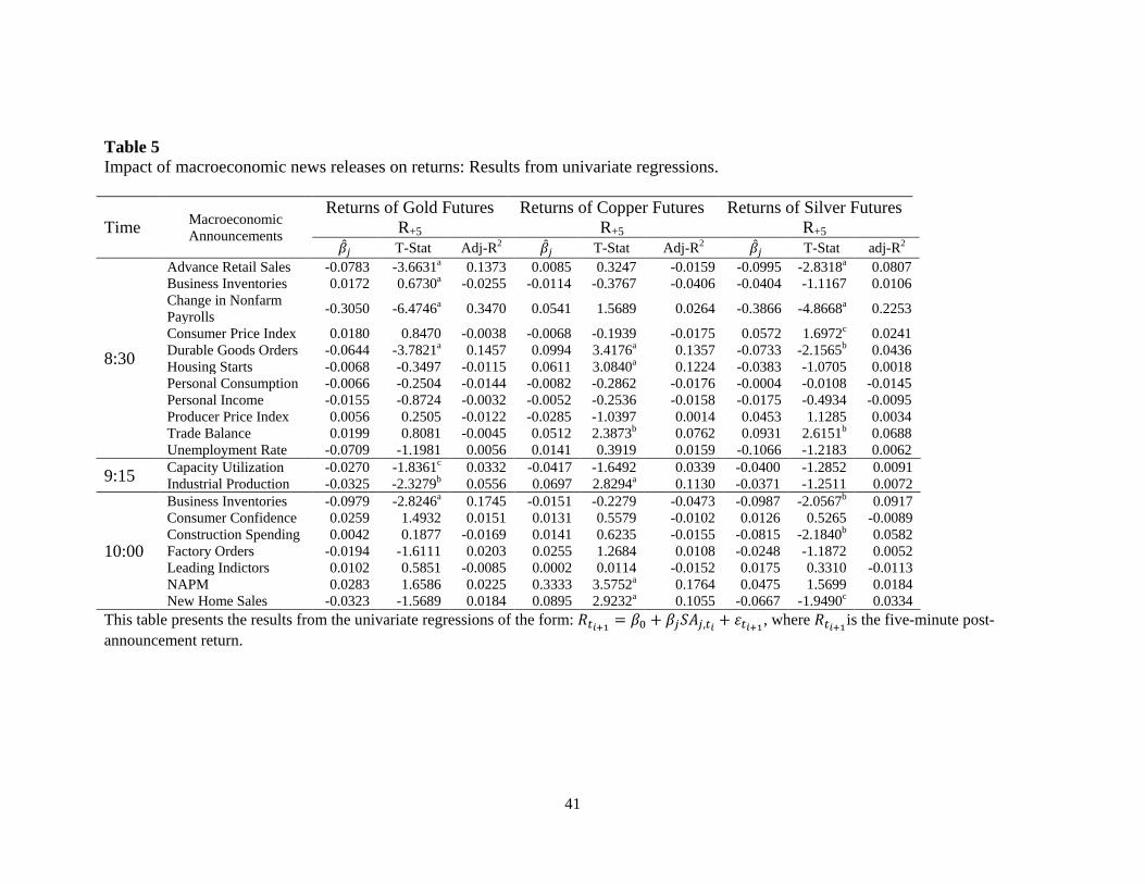
Table 5 reports estimated coefficients with corresponding t-statistics, p-values and adjusted

R-squares obtained from the individual regression models. The results are discussed first for the

8:30 announcement, followed by the 9:15 and 10:00 announcements. We notice that several 8:30

announcements have a significant impact on gold, copper and silver prices. All three metal prices

are sensitive to surprises in durable goods orders, but in different ways. In particular, durable

goods order has a negative influence on gold and silver prices, but is positively associated with

copper prices. In interpreting the coefficient values it is worth pointing out that the numbers

measure the response of the five-minute post-announcement return to a one standard deviation

change in the surprise element of the news. For instance, the �̂�𝑆𝐷𝐺𝑂 = −0.0644 coefficient value

18

for gold implies that a one standard deviation unexpected increase (decrease) in durable goods

orders causes a decrease (increase) in the price of gold futures by about 0.06% in the five

minutes after the announcement. In terms of adjusted R-square values, among the various 8:30

announcements, the nonfarm payroll indicator has the highest degree of explanatory power in the

regressions for gold (35%) and silver (23%). The importance of payroll information has been

documented in earlier studies such as Andersen and Bollerslev (1998) who refer to the

Employment Situation or Jobs Report as the “king” of all announcements because of the

significant sensitivity of most asset prices to its public release. We also observe advance retail

sales to have a strong influence on gold and silver; whereas, trade balance figures prominently in

explaining copper and silver returns. Interestingly, we find silver to be the most responsive to the

8:30 news releases with 4 out of 11 announcements having a significant impact on prices.

Finally, housing starts surprises have a positive and significant influence only on copper returns.

An evaluation of the 9:15 announcements indicates that both capacity utilization and

industrial production have a negative influence on gold returns. The estimated coefficients of the

two announcements are respectively -0.027 (regression adjusted R2 = 3.32%) and -0.0325

(regression adjusted R2 = 5.56%) and are statistically significant at the 10% level or lower. In the

case of copper, only industrial production has an influence on copper. Notably, the 9:15

announcements do not have an impact on silver returns.

Among the 10:00 announcements, business inventories have the highest degree of

explanatory power for gold and silver returns with adjusted R-square values of 17.5% and

9.17%, respectively. Surprises in business inventories have a negative impact on both gold and

silver returns. In the case of copper, however, returns in this market are positively and

19

significantly influenced by NAPM and new home sales announcements. Again, as in the 8:30

announcements, silver prices are the most sensitive to the 10:00 set of announcements.

The results in Table 5 provide meaningful insights into the nature of the relationship between

economic announcements and returns. First, announcements that reflect an unexpected

improvement in the economy tend to have a negative impact on gold and silver prices, but a

positive effect on copper. For instance, a better than expected economic growth as conveyed by

improvements in real activity (e.g., advance retail sales), consumption (e.g., new home sales) and

investment (e.g., durable goods orders) has a negative effect on gold and silver prices. One

possible explanation for this behavior is that an unexpected improvement in the economy may

reduce investors’ appetite for precious metals as they seek alternative investments such as stocks

and bonds that appear to be relatively more attractive in this environment. On the other hand,

copper returns are positively related with economic growth variables (e.g., durable goods orders,

housing starts, NAPM). This may be attributed to the fact that copper is an important input good

in manufacturing and production related industries (about 70% of the demand for copper comes

from electrical and construction industries), and a more sanguine economic climate would be

indicative of greater demand for this industrial metal.

In the next step of the empirical analysis we fit a multivariate regression model of the form:

𝑅𝑡𝑖+1 = 𝑐 + ∑ 𝛽𝑗𝑆𝐴𝑗,𝑡𝑖𝑁𝑗=1 + 𝜀𝑡𝑖+1. (3)

To estimate equation (3), we pool together all days with at least one 8:30 (9:15, 10:00)

announcement together to form the 8:30 (9:15, 10:00) study sample. In addition to estimating the

full model, we also estimate a stepwise regression model that identifies a restricted set of

regressors in the joint model with the most influential factors. For the purpose of discussion, only

20

the stepwise results are reported in the paper.7 Stepwise regressions allow some or all of the

independent variables in a standard linear multivariate regression to be chosen automatically

from a set of variables.8 However, in order to ensure that the stepwise approach does not lead to

model over-fitting and result in falsely eliminating influential variables with less significant

relationships at the start of the stepwise selection procedure, we check for consistency of the

stepwise coefficients both with the univariate model and the full joint regression model

containing all economic variables in the system. We also allow for manual additions of selected

factors from economic categories that are not represented in the stepwise approach.

The stepwise regression results, which are reported in Table 6, are largely consistent with the

univariate regression results discussed earlier. Remarkably, variables that were identified to be

influential in the univariate regressions are also found to be significant in the multivariate

regressions. We find that the 8:30 set of announcements have the largest impact on gold and

silver prices (adjusted R-square values of 23.11% and 14.93%, respectively); whereas, the 9:15

and 10:00 announcements are relatively more influential for copper (adjusted R-squares of

28.33% and 6.21%, respectively). Among the 8:30 announcements, nonfarm payrolls and

durable goods orders seem to clearly dominate the price changes on all three metals.

7 The joint regression model results can be obtained from the authors. 8 Our stepwise regressions are performed by using the stepwise-forwards method. The stepwise-forwards begins with no additional regressions in the regression, then adds the variable with the lowest p-value. The variable with the next lowest p-value given that the first variable has already been chosen, is then added. Next both of the added variables are checked against the backwards p-value criterion. Any variable whose p-value is higher than the criterion is removed. Once the removal step has been performed, the next variable is added. At this, and each successive addition to the model, all the previously added variables are checked against the backwards criterion and possibly removed. The stepwise-forwards routine ends when the lowest p-value of the variables not yet included is greater than the specified forward stopping criteria. We choose both the forward and backward criteria to be 10%. While such methods are subject to pretest bias, we still view the results as informative in their tendency to highlight variables with the greatest explanatory power.

21

5.3.2. Response of volatility and volume

This section discusses results of the impact of macroeconomic news release on realized volatility

and trading volume for the three metals. To examine volatility, we again fit joint regression

models along with their stepwise forms for the realized volatility of each metal return series. For

the sake of brevity only the reduced stepwise regression results are reported and discussed. In the

case of trading volume we are able to estimate only the stepwise regression. This is because the

joint regression models face a singularity problem due to a limited number of observations

(volume data covers 2007 and 2008) and a relatively large number of regressors. The joint

regression model has the following expression:

𝑌𝑡𝑖+1 = 𝛽0 + ∑ 𝛽𝑗𝐴𝐵𝑆(𝑆𝐴𝑗,𝑡𝑖)𝑁𝑗=1 + ∑ 𝛾𝑠3

𝑠=0 𝑌𝑡𝑖−𝑠 + 𝜀𝑡𝑖+1 (4)

where, 𝑌𝑡𝑖+1 denotes the realized volatility or volume during the 𝑖 + 1 five-minute interval at day

𝑡 when there is at least one announcement, and 𝐴𝐵𝑆(𝑆𝐴𝑗,𝑡𝑖) refers to the absolute value of the

surprise of the 𝑗𝑡ℎ announcement. To control for the persistence in volatility and volume, we

include three lags of the left hand side variable as regressors.9

The estimated results of the stepwise regression models for the realized volatility are

presented in Table 7. Several interesting observations emerge. First, among the 19 different types

of announcements, unanticipated news in nonfarm payroll has the greatest impact on the

volatility of all three markets. A one standard deviation absolute unexpected shock in nonfarm

payroll results in a 0.14%, 0.08% and 0.20% size increase in the realized volatilities of gold,

copper and silver returns, respectively. Recall that the means of the five-minute realized

volatility during the 8:30-8:35 interval in the control samples are only 0.12%, 0.14% and 0.23%

9 Notice that for returns we do not include the lagged dependent variables since returns do not exhibit persistence. For volume and volatility, however, we find the persistence parameter to be statistically significant in all our regressions. Since the focus of our discussion is on new impact variables these coefficient values are not reported; however, they may be obtained from the authors upon request.

22

for the gold, copper and silver futures returns. Viewed in this context, increases in volatility

caused by nonfarm payrolls are about 116%, 57% and 87% of the magnitudes of the

corresponding means in the three markets. Second, the announcements explain the largest

fraction of variation in gold volatility, with adjusted R-square values about 35% for the 8:30 and

9:15 announcements, and 23% for the 10:00 announcements. Third, economic news

announcements are generally associated with elevated levels of volatility, as thirteen of the

seventeen reported coefficients are positive.

Using volume data for the two year period 2007 and 2008, the stepwise models identify that,

in all instances, the reported announcements have a positive influence on trading volume (Table

8). We interpret these results are most consistent with the model of informed trading depicted by

Kim and Verrecchia (1994), in which informed traders tend to have an advantage in processing

new information after it is released, rather than in predicting new information. Once again, as in

the volatility regression, the twin 8:30 announcements of nonfarm payroll and unemployment

rate dominate the announcement shocks. For instance, a one standard deviation shock in nonfarm

payroll results in the transaction volume of gold to increase by about 900 contracts in the five

minutes following the announcement. Comparatively, the average trading volume during the

entire 8:30-8:35 for all the days in the control sample is only about 959 contracts. Similarly, the

volume in the silver contract increases by 218 contracts during this interval compared to an

average volume of only about 326 contracts in the control sample. We should note, however, that

none of the 9:15 announcements are significant in any of the volume regressions.

5.4. Persistence of announcement shocks on returns, volatility and volume

The regression results thus far provide evidence on the immediate post-announcement five-

minute interval response of gold, silver and copper. In this section, we expand the announcement

23

window to investigate the persistence of announcement shocks on returns, volatility and volume.

Specifically, we run a series of regressions at 5-minute intervals, spanning 10 minutes before the

announcement and up to 40 minutes after the announcement, and obtain the adjusted R-square

values. The R-square values from the regression are then plotted across time to interpret the

persistence of announcement shocks. Figures 3, 4 and 5 report this evidence for returns, volatility

and volume.

An overview of Figure 3 suggests that the impact of news announcements on returns

dissipates very quickly. Notably, during the 8:30-8:35 minute interval, the highest adjusted R-

square values are found for gold and silver. In contrast, copper exhibits a somewhat delayed

response to the 8:30 announcement. For the 9:15 announcements, there is about a 30-minute

delay before the realization of the highest adjusted R-square for gold and silver. This might

explain why we were unable to substantiate a post-announcement effect on returns for these two

metals. Copper prices, on the other hand, seem to incorporate the 9:15 announcements quite

rapidly. For the 10:00 announcements, the highest adjusted R-squares for gold and copper

regressions is realized during the immediate aftermath of the announcement, whereas there is

about a 5-10 minute delay in the peak response of silver prices. In all cases, we observe that the

metal prices are efficient in incorporating new economic information and the response tends to

dissipate in less than an hour after the release of the announcement. Importantly, these results

provide an interesting contrast to studies that use low frequency observations and document the

sluggish price responsiveness of commodities.

Similar to Figure 3, the evidence from shocks to volatility and volume – Figures 4 and 5,

respectively – also paints a picture where both market activity variables are responsive to

announcements. However, compared to returns, there tends to be far more persistence in

24

volatility and volume shocks (particularly with 9:15 and 10:00 announcements) suggesting that

these two variables are characterized by different properties. Again, in most cases, shocks seem

to dissipate within 60 minutes after the news release.

5.5. Asymmetric impact of news on returns, volatility and volume

We have thus far investigated the differential effects, intensity and speed of macroeconomic

shocks. The regression results implicate several announcements, chiefly nonfarm payroll and

durable goods orders, as having a disproportionate influence in the metals market. The presence

of asymmetric response, where the impacts of positive surprises and negative surprises cancel

each other, may be one possible reason as to why some announcements are not found to be

significant. In this section, we examine the differential or asymmetric response of returns,

realized volatility, and volume to positive versus negative positive economic surprises by

running a multivariate regression model of the following form:

𝑌𝑡𝑖+1 = 𝑐 + ∑ 𝛽𝑗+𝑆𝐴𝑗,𝑡𝑖+𝑁

𝑗=1 + ∑ 𝛽𝑗−𝑆𝐴𝑗,𝑡𝑖−𝑁

𝑗=1 + ∑ 𝛾𝑠𝑌𝑡𝑖−𝑠3𝑠=0 + 𝜀𝑡𝑖+1, (5)

where, 𝑌𝑡𝑖+1 denotes the return, realized volatility or volume during the 𝑖 + 1 five-minute interval

at day 𝑡 when there is at least one announcement, and 𝑆𝐴𝑗,𝑡𝑖+ , and 𝑆𝐴𝑗,𝑡𝑖

− refer to the positive and

negative components of the surprise of the 𝑗𝑡ℎ announcement. Based on our setup, there are two

possible ways in which asymmetries can be observed: (1) both negative and positive surprises

have significant impacts, but the magnitudes of their impacts are statistically different from each

other, that is, |𝛽𝑗−| ≠ |𝛽𝑗+| (a Wald test is conducted to render judgment on the equality of the

two coefficients); (2) only either negative or positive surprises are statistically significant, that is,

𝛽𝑗− = 0,𝛽𝑗+ ≠ 0, or 𝛽𝑗− ≠ 0,𝛽𝑗+ = 0 , in which case this would automatically indicate the

presence of an asymmetric response. We estimate the full regression model, but report only its

stepwise counterpart in Tables 9 through 11.

25

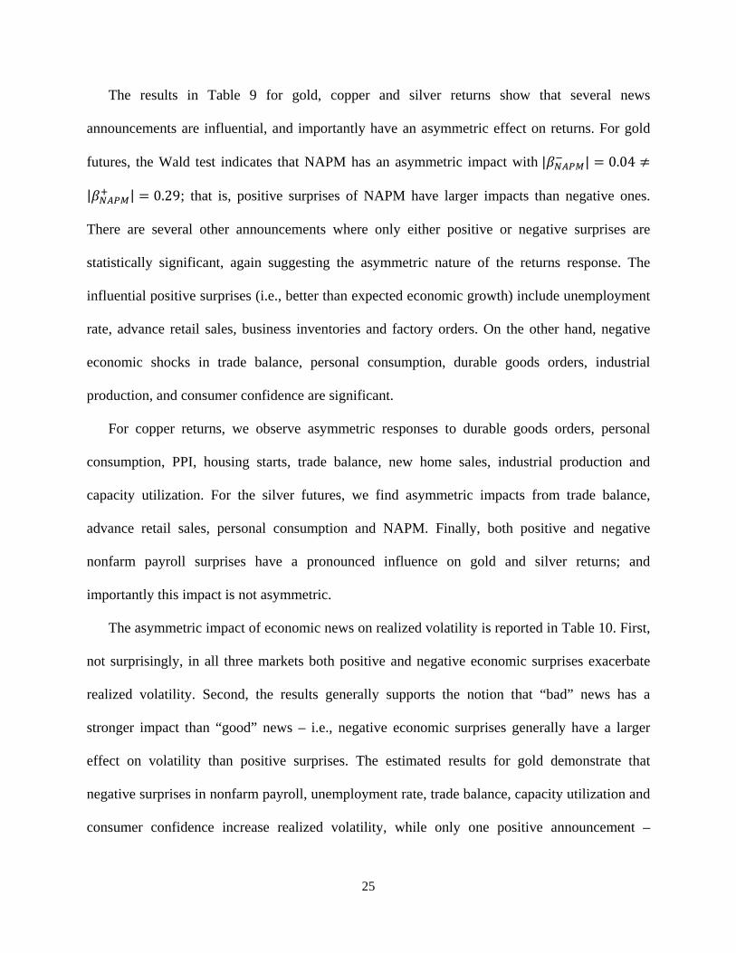
The results in Table 9 for gold, copper and silver returns show that several news

announcements are influential, and importantly have an asymmetric effect on returns. For gold

futures, the Wald test indicates that NAPM has an asymmetric impact with |𝛽𝑁𝐴𝑃𝑀− | = 0.04 ≠

|𝛽𝑁𝐴𝑃𝑀+ | = 0.29; that is, positive surprises of NAPM have larger impacts than negative ones.

There are several other announcements where only either positive or negative surprises are

statistically significant, again suggesting the asymmetric nature of the returns response. The

influential positive surprises (i.e., better than expected economic growth) include unemployment

rate, advance retail sales, business inventories and factory orders. On the other hand, negative

economic shocks in trade balance, personal consumption, durable goods orders, industrial

production, and consumer confidence are significant.

For copper returns, we observe asymmetric responses to durable goods orders, personal

consumption, PPI, housing starts, trade balance, new home sales, industrial production and

capacity utilization. For the silver futures, we find asymmetric impacts from trade balance,

advance retail sales, personal consumption and NAPM. Finally, both positive and negative

nonfarm payroll surprises have a pronounced influence on gold and silver returns; and

importantly this impact is not asymmetric.

The asymmetric impact of economic news on realized volatility is reported in Table 10. First,

not surprisingly, in all three markets both positive and negative economic surprises exacerbate

realized volatility. Second, the results generally supports the notion that “bad” news has a

stronger impact than “good” news – i.e., negative economic surprises generally have a larger

effect on volatility than positive surprises. The estimated results for gold demonstrate that

negative surprises in nonfarm payroll, unemployment rate, trade balance, capacity utilization and

consumer confidence increase realized volatility, while only one positive announcement –

26

nonfarm payrolls– significantly increases volatility. Also, note that the 8:30 announcements

again dominate, with only one of the 9:15 announcements containing sufficient information to

cause volatility to increase.

The estimated results for copper demonstrate that several announcements – nonfarm payrolls,

personal income, personal consumption, PPI, housing starts and NAPM – have an asymmetric

impact on realized volatility. In the case of silver, many announcements that were found to have

an asymmetric impact on gold volatility also have an asymmetric effect on silver volatility.

Furthermore, Wald test for the equality of trade balance coefficients suggest that the magnitude

of negative surprises is about 3 times that of positive surprises (𝛽𝑇𝐵+ = 0.0405 , 𝛽𝑇𝐵− =

−1.5636).

The asymmetric impact on trading volume is presented in Table 11. In general, volume in all

three metals is higher in the immediate aftermath of both positive and negative news

announcements. Overall, the prominence of unemployment rate and nonfarm payroll surprises is

substantiated.

6. A simple trading rule10

Our analysis so far reveals that news releases have a strong and instantaneous impact on all three

metals. In the current section we extend this general finding to examine if the direction of the

macroeconomic surprise can be used to construct a profitable metal futures trading strategy. The

strategy is based on a simple set of rules:

a. There are no trades initiated on days where there are no scheduled macroeconomic

news releases.

b. On days when there is a scheduled news release, a long or short position is held over

a 5-minute interval, depending on the direction of the surprise. The direction of the 10 This section is an extension of the original paper.

27

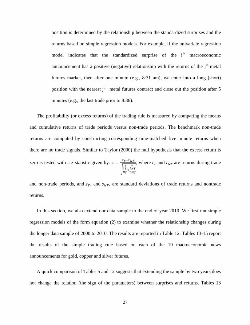
position is determined by the relationship between the standardized surprises and the

returns based on simple regression models. For example, if the univariate regression

model indicates that the standardized surprise of the ith macroeconomic

announcement has a positive (negative) relationship with the returns of the jth metal

futures market, then after one minute (e.g., 8:31 am), we enter into a long (short)

position with the nearest jth metal futures contract and close out the position after 5

minutes (e.g., the last trade prior to 8:36).

The profitability (or excess returns) of the trading rule is measured by comparing the means

and cumulative returns of trade periods versus non-trade periods. The benchmark non-trade

returns are computed by constructing corresponding time-matched five minute returns when

there are no trade signals. Similar to Taylor (2000) the null hypothesis that the excess return is

zero is tested with a z-statistic given by: 𝑧 = �̅�𝑇−�̅�𝑁𝑇

�𝑠𝑇2

𝑛𝑇+𝑠𝑁𝑇2

𝑛𝑁𝑇

, where �̅�𝑇 and �̅�𝑁𝑇 are returns during trade

and non-trade periods, and 𝑠𝑇, and 𝑠𝑁𝑇, are standard deviations of trade returns and nontrade

returns.

In this section, we also extend our data sample to the end of year 2010. We first run simple

regression models of the form equation (2) to examine whether the relationship changes during

the longer data sample of 2000 to 2010. The results are reported in Table 12. Tables 13-15 report

the results of the simple trading rule based on each of the 19 macroeconomic news

announcements for gold, copper and silver futures.

A quick comparison of Tables 5 and 12 suggests that extending the sample by two years does

not change the relation (the sign of the parameters) between surprises and returns. Tables 13

28

through 15 provide detailed results associated with the trading strategy for gold, copper and

silver futures. Table 16 summarizes the aggregate profits for each of the three futures contracts

for each macroeconomic announcement. The results show that this simple trading rule generates

substantial profits. The difference between trade and non-trade returns for several

announcements is both statistically significant as indicated by the z-statistic and economically

significant as suggested by the magnitude of returns.11 In particularly, for both gold and silver,

applying this rule to the change in nonfarm payroll generates profit of 20.7% and 24.4%,

respectively, and applying the rule to trade balance and advanced retail sales announcements

generates profits 6.5% and 5.1% and 6.7% and 7.8%, respectively. For copper, the most

significant trading profits are generated by new home sales (10.6%) followed by consumer

confidence (9.8%), durable goods (8.6%) and change in nonfarm payroll (8.0%).

For comparison, we also calculate trading profits at 5-minute intervals throughout the trading

day. These results suggest that the primary opportunity to generate abnormal profits is in the first

5-minutes after the announcement (after the one-minute delay).12 As an illustration, we report

these results in Figure 6 for the change of nonfarm payroll announcement. Figure 6 reports the

mean of long, short and nontrade days at five minute intervals from 8:31 to the close of the

futures markets (13:30 for gold, 13:00 for copper and 13:25 for silver). For all three markets,

both long and short positions during the 8:31-8:35 interval generate the greatest mean return. The

means then decrease dramatically over the subsequent 5-minute interval. Notably, the means of

11 The reported returns would be amplified if we accounted for the high leverage associated with trading futures contracts (about 23:1 for GC, 20:1 for HG and 9:1 for SI). The initial margin requirements as of July 2011 are: $6,751 per GC contract (100 Troy Ounces of gold, roughly $160,000), $5,378 per HG contract (25,000 pounds of grade 1 copper, roughly $111,000), and $21,600 per SI contract (5,000 Troy ounces of silver, roughly $200,000). Since our trading strategy is predicated on an intraday trading rule maintenance margin requirements are not important. We should note that, in calculating trading rule profits we do not account for bid-ask spreads. We do not expect this to be material however, given that (a) we document returns that are quite large in magnitude; and (b) we compare returns with a non-trade sample. 12 Results are available upon requirement.

29

the long positions are greater than the means of the short positions for both gold and silver.

Since precious metals have a negative relationship with nonfarm payrolls, this indicates that bad

news generates greater returns than good news. For copper, the mean of the long positions during

the period of 8:31-8:35 is still the greatest among all the five minute long positions. Interestingly,

the mean of the long positions during the period of 8:36-8:40 is the lowest. This suggests that

copper prices initially overreact to positive surprises in nonfarm payrolls, and then overcorrect in

the subsequent 5-minute interval. This pattern repeats several times before approaching the

means over the nontrading days at about 9:30.

In sum, our results in Tables 13-16 indicate that this trading strategy generates substantive

profits. Figure 6 suggests that any trading rule to exploit the information content of news

announcements would likely be concentrated in the first five minutes after the announcement.

7. Concluding remarks

The question of whether commodity prices are influenced by macroeconomic fundamentals or

whether they are predetermined with respect to monetary aggregates is a topic that has yet to find

consensus. Although there are strong economic reasons to expect commodity prices to be

sensitive to macroeconomic fundamentals, prior empirical studies have not been very successful

in documenting a strong relationship. We suggest that this might be due to several reasons

including measurement of data at low (daily or monthly) frequencies and research methods that

do not control for asymmetric impacts.

We undertake a comprehensive examination of the response of return, volatility and trading

volume for gold, copper and silver to 19 different types of macroeconomic announcements.

Notably, we rely on an improved analytical framework that uses high-frequency data for a

sample period spanning 7 years from 2002 to 2008. The announcements are classified by time

30

and direction (i.e., whether the news release signals better-than-expected-economic news or

worse-than-expected news) in order to: (a) identify the most important set of announcements; (b)

trace the persistence of macroeconomic shocks; and (c) allow for asymmetry in the relationships.

Our analysis reveals that news releases have a strong and instantaneous impact on all three

metals. First, the 8:30 set of announcements appear to have the largest impact on prices, realized

volatility and trading volume during the immediate post-announcement five minute interval. For

instance, univariate regression models show that surprises in nonfarm payroll (released at 8:30

am) explain about 35% and 23% of the returns of gold and silver, respectively during the 8:30 to

8:35 time interval. Copper returns, on the hand, are more sensitive to the 9:15 set of

announcements which include capacity utilization and industrial production. The evidence

suggests that the behavior of commodity markets is quite similar to other asset markets in terms

of their responsiveness to economic information. Our results for volume are most consistent with

informed trading models where informed traders tend to have an advantage in processing, rather

than predicting, new information.

Second, our results indicate that the metals markets respond in an economically predictable

manner. Unexpected improvement in economic growth has a negative impact on gold and silver

prices, but registers a favorable effect on copper returns. For instance, improvements in real

economic activity (e.g., advance retail sales), consumption (e.g., new home sales) and investment

(e.g., durable goods orders) are found to negatively influence gold and silver prices. The

performance of copper, on the other hand, is consistent with its status as an important industrial

metal that benefits primarily from unexpected growth in the economy.

Third, our evidence indicates that the effect of macroeconomic news dissipates quickly,

within about 60 minutes of the news release, and notably, and that several announcements have

31

an asymmetric impact on market activity variables. These results provide an insightful contrast to

previous studies that use daily data to examine the relationship between macroeconomic news

and commodity prices.

Finally, we show that significant trading profits can be generated in all three metal futures

markets by following a simple five minute trading rule that is based on the direction of the

macroeconomic news surprise.

32

References Adams, G., McQueen, G., Wood, R., 2004. The effects of inflation news on high frequency stock returns. Journal of Business 77, 547-574. Andersen, T.G., 1996. Return volatility and trading volume: An information flow interpretation of stochastic volatility. Journal of Finance 51, 169–204. Andersen, T.G., Bollerslev, T., 1998. DM-dollar intraday volatility: Activity pattern, macroeconomic announcemnets, and longer run dependences. Journal of Finance 53, 219-265. Barndorff-Nielsen, O.E., Shephard, N., 2002. Econometric analysis of realized volatility and its use in estimating stochastic volatility models. Journal of the Royal Statistical Society, Series B 64, 253-280. Baur, D.G., Lucey, B.M., 2010. Is gold a hedge or a safe haven? An analysis of stocks, bonds and gold. Financial Review 45, 217-229. Brennan, M., 1958. The supply of storage. American Economic Review 48, 934-941. Boyd, J.H., Hu, J., Jagannathan, R., 2005. The stock market’s reaction to unemployment news: Why bad news is usually good for stocks. Journal of Finance 60, 647-672. Cai, J., Cheung, Y.L., Wong, M.C.S., 2001. What moves the gold market? Journal of Futures Markets 21, 257-278. Chen, N., Roll, R., Ross, S., 1986. Economic forces and the stock market. Journal of Business 59, 383-403. Chen, Y.L., Gau, Y.F., 2010. News announcements and price discovery in foreign exchange spot and futures markets. Journal of Banking and Finance 34, 1628-1636. Christie-David, R., Chaudhry, M., Koch, T.W., 2000. Do macroeconomic news releases affect gold and silver prices? Journal of Economics and Business 52, 405-421. Ederington, L.H., Lee, J.H., 1993. How markets process information: News releases and volatility. Journal of Finance 48, 1161-1191. Erb, C., Harvey, C., 2006. The tactical and strategic value of commodity futures. Financial Analysts Journal 62, 69-97. Flannery, M. J., Protopapadakis, A., 2002. Macroeconomic factors do influence aggregate stock returns. Review of Financial Studies 15, 751-782. Glosten, L.R., Milgrom, P.R., 1985. Bid, ask and transaction prices in a specialist market with heterogeneously informed traders. Journal of Financial Economics 14, 71-100.

33

Hansen, P. R, Lunde, A., 2006. Realized Variance and Market Microstructure Noise. Journal of Business & Economic Statistics 24, 127-161. Hess, D., Huang, H., Niessen, A., 2008. How do commodity futures response to macroeconomic news? Financial Markets and Portfolio Management 22, 127-146. Khalifa, A.A., Miao, H., Ramchander, S., 2011. Return distributions and volatility forecasting in metal futures markets: Evidence from gold, silver, and copper. Journal of Futures Markets 31, 55-80. Kilian, L., Vega, C., 2010. Do energy prices respond to U.S. macroeconomic news? A test of the hypothesis of predetermined energy prices. Review of Economics and Statistics 93, 660-671. Kim, O., Verrecchia, R., 1994. Market liquidity and volume around earnings announcements. Journal of Accounting and Economics 17, 41–67. Kocagil, A., 1997. Does futures speculation stabilize spot prices? Evidence from metal markets. Applied Financial Economics 7, 113-125. Koutmos, G., Booth, G.G., 1995. Asymmetric volatility transmission in international stock markets. Journal of International Money and Finance 14, 747-762. Maheu, J.M., McCurdy, T.H., 2011. Do high-frequency measures of volatility improve forecasts of return distributions? Journal of Econometrics 160, 69-76. Nowak, S., Andritzky, J., Jobst, A., Tamirisa, N., 2011. Macroeconomic fundamentals, price discovery, and volatility dynamics in emerging bond markets. Journal of Banking and Finance, forthcoming. Pasquariello, P., Vega, C., 2007. Informed and strategic order flow in the bond markets. Review of Financial Studies 20, 1975-2019. Roache, S.K., Rossi, M., 2010. The effects of economic news on commodity prices: Is gold just another commodity. The Quarterly Review of Economics and Finance 50, 377-385. Ross, S.A., 1989. Information and volatility: The no-arbitrage martingale approach to timing and resolution irrelevancy. Journal of Finance 44, 1–18. Simpson, M.W., Ramchander, S., 2004. An examination of the impact of macroeconomic news on the spot and futures treasuries markets. Journal of Futures Markets 24, 453-478. Simpson, M.W., Ramchander, S., Chaudhry, M., 2005. The impact of macroeconomic surprises on spot and forward exchange markets. Journal of International Money and Finance 24, 693-718.

34

Tauchen, G.E., Pitts, M., 1983. The price variability-volume relationship on speculative markets. Econometrica 51, 485-505. Working, H., 1949. The theory of price of storage. American Economic Review 30, 1254-1262.

35

Table 1 Summary statistics of daily raw returns (percentages) for the period 2002-2008.

Gold Futures Copper Futures Silver Futures Mean 0.0653 0.0426 0.0511 Median 0.0897 0.0611 0.1857 Standard Deviation 1.2339 1.9992 2.1158 Skewness -0.2635 -0.4042 -1.0500 Kurtosis 6.9825 7.6518 10.3024 Jarque-Bera 1188.18 1635.69 4246.01 Probability 0.0000 0.0000 0.0000 No. of observations 1767 1761 1765

36

Table 2 List of U.S. macroeconomic news announcements: 2002-2008.

Time Announcements (Abbreviation) Total Std. Dev. of Surprise Components

8:30 Advance Retail Sales (ARS) 84 0.1582 8:30 Business Inventories2 (BI) 35 2.5123 8:30 Change in Nonfarm Payrolls (CNP) 84 108.2439 8:30 Consumer Price Index (CPI) 84 78.8039 8:30 Durable Goods Orders (DGO) 84 0.7946 8:30 Housing Starts (HS) 84 0.2892 8:30 Personal Consumption1 (PC) 72 0.5486 8:30 Personal Income (PI) 84 0.5121 8:30 Producer Price Index (PPI) 84 55.9627 8:30 Trade Balance Goods & Services (TB) 84 0.1434 8:30 Unemployment Rate (UR) 84 0.2281 9:15 Industrial Production (IP) 84 0.3989 9:15 Capacity Utilization (CU) 84 0.3350 10:00 Business Inventories2 (BI) 49 14.3884 10:00 Construction Spending (CS) 84 0.5556 10:00 Consumer Confidence (CC) 84 0.6866 10:00 Factory Orders (FO) 84 8.0338 10:00 Leading Indicators (LI) 84 0.1787 10:00 NAPM 84 77.2018 10:00 New Home Sales (NHS) 84 0.2281

Total 1,584 This table lists the 19 different types of macroeconomic announcements along with the standard deviation of the surprise component. The surprise component is measured by: Surprise = Actual – Forecast. (For personal consumption, we only have data from 2003. For business inventories, some of the announcements were at 8:30 and others at 10. )

37

Table 3 Analysis sample.

Market Study Sample Control Sample 8:30 9:15 10:00 8:30 9:15 10:00

Gold 609 (169) 83 (21) 428 (135) 751 (197) 751 (197) 751 (197) Copper 475 (101) 63 (10) 335 (86) 605 (139) 605 (139) 605 (139) Silver 630 (177) 85 (22) 437 (137) 772 (220) 772 (220) 772 (220) This table reports the total number of observations in the study sample and control sample for the 8:30, 9:15, and 10:00 announcements. The numbers in parenthesis are the number of days in the trading volume sample. We have volume data only for 2007 and 2008.

38

Table 4 Test of equality in mean return, realized volatility and volume around announcements. Panel A: Tests of equality in means of returns, realized volatility and volume around macroeconomic announcements for gold futures.

Gold Futures Sample

8:30 Announcement

Test of Equality in Means

9:15 Announcement

Test of Equality in Means

10:00 Announcement

Test of Equality in Means

8:25- 8:30

8:30- 8:35

Welch’s t-test 9:10- 9:15

9:15- 9:20

Welch’s t-test 9:55- 10:00

10:00- 10:05

Welch’s t-test

Returns

Control 0.0096 0.0028 -0.9258 0.0001 0.0024 0.3924 -0.0108 -0.0228 -1.8972c Study 0.0107 0.0132 0.2124 -0.0244 0.0026 1.3242 -0.0096 -0.0235 -1.5006 Difference 0.0011 0.1568 -0.0245 -1.5699 0.0012 0.1706 Difference 0.0104 0.8743 0.0002 0.0181 -0.0007 -0.0782

Realized Volatility

Control 0.1107 0.1156 1.1692 0.0919 0.0970 1.5205 0.0943 0.1051 3.1516a Study 0.1070 0.1986 13.1942a 0.0974 0.1301 2.9071a 0.0995 0.1356 7.0058a Difference -0.0037 -0.8739 0.0055 0.7344 0.0052 1.2822 Difference 0.083 12.0259a 0.0331 3.6890a 0.0305 6.5528a

Volume

Control 1054.70 959.35 -1.0237 843.61 835.23 -0.1204 983.62 1135.05 1.5731 Study 843.25 1713.41 7.5141a 1134.67 1149.91 0.0408 1015.24 1384.46 3.2180a Difference -211.45 -2.3911b 291.06 0.9967 31.62 0.3342 Difference 754.06 6.3135a 314.68 1.2943 249.41 2.1719b

This table reports tests of equality in means of returns, realized volatilities, and volume around the announcements intervals at 8:30, 9:15 and 10:00 for gold, copper and silver. The returns, realized volatilities, and volumes are calculated over five minute intervals before and after the announcement time points. Tests for equality in means between the returns, realized volatilities and volumes before and after the announcements are reported for both the control sample and the study sample. We also report tests of equality between the control and study samples, both prior to and after the announcement. The Welch’s t-test, sometimes called “Satterthwaite-Welch t-test”, allows for unequal cell variances in samples. In our case, the p-values of the Welch’s t-test are only slightly higher than the standard t-test. The returns and volatilities are expressed in percentages (i.e., multiplied by 100).

39

Panel B: Tests of equality in means of returns, realized volatility and volume around macroeconomic announcements for copper futures.

Copper Futures Sample

8:30 Announcement

Test of Equality in Means

9:15 Announcement

Test of Equality in Means

10:00 Announcement

Test of Equality in Means

8:25- 8:30

8:30- 8:35

Welch’s t-test 9:10- 9:15

9:15- 9:20

Welch’s t-test 10:00- 10:05

10:00- 10:05

Welch’s t-test

Returns

Control -0.0033 -0.0061 -0.2680 0.0058 -0.0084 -1.7108b 0.0020 -0.0100 -1.4081 Study -0.0126 0.0101 1.7279c 0.0243 -0.0394 -2.5287b -0.0102 -0.0022 0.5448 Difference -0.0093 -0.8581 0.0185 1.0417 -0.0122 -1.0472 Difference 0.0162 1.2627 -0.031 -1.5679 0.0078 0.6372

Realized Volatility

Control 0.1380 0.1407 0.4435 0.1096 0.1065 -0.5579 0.1026 0.1137 1.8867 Study 0.1429 0.1893 6.5357a 0.0957 0.1206 1.5389 0.1054 0.1380 3.9413a Difference 0.0049 0.8211 -0.0139 -1.3359 0.0028 0.3817 Difference 0.0486 6.7665a 0.0141 1.0390 0.0243 3.5036a

Volume

Control 114.04 124.01 0.7042 92.97 95.04 0.2095 87.40 98.23 1.2372 Study 88.70 129.99 3.0905a 83.50 92.10 0.3947 90.22 114.93 1.7539c Difference -25.34 -2.1245b -9.47 -0.5521 2.82 0.3089 Difference 5.98 0.3881 -2.94 -0.1762 16.70 1.2057

40

Panel C: Test of equality in means of return, realized volatility and volume around macroeconomic announcements for silver futures.

Silver Futures Sample

Means Around 8:30

Test of Equality in Means

Means Around 9:15

Test of Equality in Means

Means Around 10:00

Test of Equality in Means

8:25- 8:30

8:30- 8:35

Welch’s t-test 9:10- 9:15

9:15- 9:20

Welch’s t-test 10:00- 10:05

10:00- 10:05

Welch’s t-test

Return

Control 0.0052 0.0081 0.1564 -0.0070 -0.0074 -0.0471 -0.0222 -0.0079 1.3387 Study 0.0137 0.0274 0.6139 0.0106 -0.0028 -0.3455 -0.0020 -0.0514 -2.6693a Difference 0.0085 0.3805 0.0176 0.6565 0.0202 1.4420 Difference 0.0193 1.0210 0.0046 0.1601 -0.0435 -2.6951a

Realized Volatility

Control 0.3153 0.2302 -7.4237a 0.1727 0.1724 -0.0491 0.1673 0.1708 0.5662 Study 0.3115 0.3355 1.7080 0.1702 0.2108 2.0718b 0.1740 0.2138 3.3465a Difference -0.0038 -0.2826 -0.0025 -0.1963 0.0067 0.8521 Difference 0.1053 8.7503a 0.0384 2.3564b 0.043 3.9404a

Volume

Control 463.07 325.86 -4.3813a 234.40 236.08 0.0982 266.13 287.19 0.9199 Study 426.57 486.19 1.9143 232.59 334.00 1.4990 284.61 346.09 1.7686b Difference -36.50 -1.2280 -1.81 -0.0434 18.48 0.6261 Difference 160.33 4.9078a 97.92 1.7466c 58.9 2.0068c

Notes: Superscripts “a”, “b” and “c” indicate significance at the 1%, 5%, and 10% levels, respectively.

41

Table 5 Impact of macroeconomic news releases on returns: Results from univariate regressions.

Time Macroeconomic

Announcements Returns of Gold Futures Returns of Copper Futures Returns of Silver Futures

R+5 R+5 R+5 �̂�𝑗 T-Stat Adj-R2 �̂�𝑗 T-Stat Adj-R2 �̂�𝑗 T-Stat adj-R2

8:30

Advance Retail Sales -0.0783 -3.6631a 0.1373 0.0085 0.3247 -0.0159 -0.0995 -2.8318a 0.0807 Business Inventories 0.0172 0.6730a -0.0255 -0.0114 -0.3767 -0.0406 -0.0404 -1.1167 0.0106 Change in Nonfarm Payrolls -0.3050 -6.4746a 0.3470 0.0541 1.5689 0.0264 -0.3866 -4.8668a 0.2253

Consumer Price Index 0.0180 0.8470 -0.0038 -0.0068 -0.1939 -0.0175 0.0572 1.6972c 0.0241 Durable Goods Orders -0.0644 -3.7821a 0.1457 0.0994 3.4176a 0.1357 -0.0733 -2.1565b 0.0436 Housing Starts -0.0068 -0.3497 -0.0115 0.0611 3.0840a 0.1224 -0.0383 -1.0705 0.0018 Personal Consumption -0.0066 -0.2504 -0.0144 -0.0082 -0.2862 -0.0176 -0.0004 -0.0108 -0.0145 Personal Income -0.0155 -0.8724 -0.0032 -0.0052 -0.2536 -0.0158 -0.0175 -0.4934 -0.0095 Producer Price Index 0.0056 0.2505 -0.0122 -0.0285 -1.0397 0.0014 0.0453 1.1285 0.0034 Trade Balance 0.0199 0.8081 -0.0045 0.0512 2.3873b 0.0762 0.0931 2.6151b 0.0688 Unemployment Rate -0.0709 -1.1981 0.0056 0.0141 0.3919 0.0159 -0.1066 -1.2183 0.0062

9:15 Capacity Utilization -0.0270 -1.8361c 0.0332 -0.0417 -1.6492 0.0339 -0.0400 -1.2852 0.0091 Industrial Production -0.0325 -2.3279b 0.0556 0.0697 2.8294a 0.1130 -0.0371 -1.2511 0.0072

10:00

Business Inventories -0.0979 -2.8246a 0.1745 -0.0151 -0.2279 -0.0473 -0.0987 -2.0567b 0.0917 Consumer Confidence 0.0259 1.4932 0.0151 0.0131 0.5579 -0.0102 0.0126 0.5265 -0.0089 Construction Spending 0.0042 0.1877 -0.0169 0.0141 0.6235 -0.0155 -0.0815 -2.1840b 0.0582 Factory Orders -0.0194 -1.6111 0.0203 0.0255 1.2684 0.0108 -0.0248 -1.1872 0.0052 Leading Indictors 0.0102 0.5851 -0.0085 0.0002 0.0114 -0.0152 0.0175 0.3310 -0.0113 NAPM 0.0283 1.6586 0.0225 0.3333 3.5752a 0.1764 0.0475 1.5699 0.0184 New Home Sales -0.0323 -1.5689 0.0184 0.0895 2.9232a 0.1055 -0.0667 -1.9490c 0.0334

This table presents the results from the univariate regressions of the form: 𝑅𝑡𝑖+1 = 𝛽0 + 𝛽𝑗𝑆𝐴𝑗,𝑡𝑖 + 𝜀𝑡𝑖+1, where 𝑅𝑡𝑖+1is the five-minute post-announcement return.

42

Table 6 Stepwise models of impact of macroeconomic news on returns.

Gold R+5 Copper R+5 Silver R+5

Optimal Regressors �̂�𝑗 T-Stat Optimal

Regressors �̂�𝑗 T-Stat Optimal Regressors �̂�𝑗 T-Stat

8:30

Intercept 0.0028 0.3063 Intercept 0.0104 1.0313 Intercept 0.0131 0.8837 CNP -0.3087 -12.819a DGO 0.0994 3.4775a CNP -0.4035 -9.8125a UR -0.1237 -4.9134a HS 0.0622 2.2294b UR -0.1611 -3.9189a ARS -0.0782 -3.1249a CNP 0.0528 1.9995b ARS -0.0989 -2.3838b DGO -0.0641 -2.4553b TB 0.0426 1.7804c TB 0.0939 2.3324b DGO -0.0715 -1.7174c Adjusted R2 0.2311 Adjusted R2 0.0412 Adjusted R2 0.1493 F-Statistics 46.6755a F-Statistics 6.0734a F-Statistics 23.0766a

9:15 Intercept -0.0012 -0.0866 Intercept -0.0454 -2.743a Intercept -0.0028 -0.0976 IP -0.0325 -2.4164b IP 0.1249 4.8263a CU -0.1140 -4.069a Adjusted R2 0.0557 Adjusted R2 0.2833 Adjusted R2 0.0000 F-Statistics 5.8390a F-Statistics 13.2520a F-Statistics

10:00 Intercept -0.0219 -2.9451a Intercept -0.0053 -0.5134 Intercept -0.0493 -3.4352a BI -0.0981 -3.3681a NHS 0.0950 3.9673a CS -0.0826 -2.1631b NAPM 0.0303 1.8045c NAPM 0.3341 2.8937a NHS -0.0642 -1.8307c NHS -0.0316 -1.7402c BI -0.1011 -1.6629c Adjusted R2 0.0331 Adjusted R2 0.0621 Adjusted R2 0.0175 F-Statistics 5.8674a F-Statistics 12.0512a F-Statistics 3.5945b

This table reports the estimated stepwise regression models for returns of the three metals. The stepwise regressions pick up only the announcements which have an impact on the returns at the 10% significance level. The stepwise regression models have the form: 𝑅𝑡𝑖+1 = 𝑐 + ∑ 𝛽𝑗𝑆𝐴𝑗,𝑡𝑖

𝑁𝑗=1 + 𝜀𝑡𝑖+1. , where 𝑅𝑡𝑖+1 is the five-minute

post-announcement return, 𝑆𝐴𝑗,𝑡𝑖 is the standardized surprise of the 𝑗𝑡ℎ announcement at time 𝑡𝑖 on day t. Superscripts “a”, “b” and “c” indicate significance at the 1%, 5%, and 10% levels, respectively. Refer to Table 2 for abbreviations for the various macroeconomic announcements.

43

Table 7 Stepwise model of impact of macroeconomic news on realized volatility. Gold RV+5 Copper RV+5 Silver RV+5

Optimal Regressors �̂�𝑗 T-Stat Optimal

Regressors �̂�𝑗 T-Stat Optimal Regressors �̂�𝑗 T-Stat

8:30

Intercept 0.0952 9.9618a Intercept 0.0852 7.4360a Intercept 0.1949 13.6505a ABS_CNP 0.1442 9.5281a ABS_CNP 0.0767 5.7166a ABS_CNP 0.1995 7.2280a ABS_UR 0.0800 5.0778a ABS_PI -0.0358 -2.7338a ABS_UR 0.1061 3.8416a ABS_BI -0.0518 -2.0028b ABS_TB 0.0420 1.7645c ABS_ARS 0.0241 1.6755c Adjusted R2 0.3576 Adjusted R2 0.2345 Adjusted R2 0.2631 F-Statistics 55.8418a F-Statistics 23.845a F-Statistics 55.7665a

9:15

Intercept 0.0407 2.2928b Intercept 0.0789 3.0725a Intercept 0.0912 3.0409a ABS_CU 0.0364 3.2618a ABS_CU -0.0638 -2.1556b ABS_IP 0.0504 1.8018c Adjusted R2 0.3483 Adjusted R2 0.2184 Adjusted R2 0.2990 F-Statistics 8.2315a F-Statistics 2.6084b F-Statistics 8.5312a

10:00

Intercept 0.0729 9.8303a Intercept 0.0663 7.7184a Intercept 0.0624 3.5262a ABS_CC 0.0377 4.7421a ABS_NAPM 0.1325 2.2288b ABS_NAPM 0.0236 2.9555a ABS_CS -0.0339 -2.1008b ABS_BI 0.0269 1.8931c Adjusted R2 0.2343 Adjusted R2 0.2702 Adjusted R2 0.1937 F-Statistics 18.3579a F-Statistics 20.2395a F-Statistics 25.9522a

This table reports the estimated stepwise regression models for the realized volatility (RV) five minutes after each announcement. The stepwise regressions pick up only the announcements which have impacts on the five-minute realized volatility at the 10% significance level. The stepwise regression models have the form: 𝑅𝑉𝑡𝑖+1 = 𝛽0 +∑ 𝛽𝑗𝐴𝐵𝑆(𝑆𝐴𝑗,𝑡𝑖)𝑁𝑗=1 + ∑ 𝛾𝑠3

𝑠=0 𝑅𝑉𝑡𝑖−𝑠 + 𝜀𝑡𝑖+1 .𝑅𝑉𝑡𝑖+1 is the post-announcement five-minute realized volatility, 𝐴𝐵𝑆(𝑆𝐴𝑗,𝑡𝑖) is the absolute value of the surprise of the 𝑗𝑡ℎ announcement, and 𝛾 is the volume persistence parameter that accounts for dependent variable lags (not reported). Superscripts “a”, “b” and “c” indicate significance at the 1%, 5% and 10% levels, respectively. Refer to Table 2 for abbreviations for the various macroeconomic announcements.

44

Table 8 Stepwise model of impact of macroeconomic news on trading volume (2007-2008). Gold V+5 Copper V+5 Silver V+5

Optimal Regressors �̂�𝑗 T-Stat Optimal

Regressors �̂�𝑗 T-Stat Optimal Regressors �̂�𝑗 T-Stat

8:30

Intercept 818.79 6.4871a Intercept 30.33 2.4878b Intercept 256.17 6.3106a ABS_UR 822.61 3.7171a ABS_UR 87.43 3.7744a ABS_UR 235.51 3.8686a ABS_CNP 902.08 2.9492a ABS_ARS 86.40 2.9954a ABS_CNP 217.68 1.9704c ABS_ARS 132.12 1.9095c Adjusted R2 0.3525 Adjusted R2 0.5586 Adjusted R2 0.2659 F-Statistics 23.2685a F-Statistics 19.8271a F-Statistics 15.5715a

9:15 Intercept 174.19 0.8291 Intercept 79.86 1.6478 Intercept 62.17 1.2393 Adjusted R2 0.7826 Adjusted R2 0.6460 Adjusted R2 0.8325 F-Statistics 15.2966a F-Statistics 2.2809 F-Statistics 21.1300a

10:00 Intercept 415.08 2.9698a Intercept 4.63 0.2490 Intercept 85.53 2.1109b ABS_NAPM 308.16 2.1120b ABS_CC 230.24 3.8882a ABS_BI 130.43 1.9295c Adjusted R2 0.3567 Adjusted R2 0.4290 Adjusted R2 0.3188 F-Statistics 14.7500a F-Statistics 12.0211a F-Statistics 12.2604a

This table reports the estimated stepwise regression models for trading volume five minutes after each announcement. The stepwise regressions pick up only the announcements which have impact on the five-minute volume at the 10% significance level. The stepwise regression models have the form: 𝑉𝑡𝑖+1 = 𝛽0 + ∑ 𝛽𝑗𝐴𝐵𝑆(𝑆𝐴𝑗,𝑡𝑖)

𝑁𝑗=1 + ∑ 𝛾𝑠3

𝑠=0 𝑉𝑡𝑖−𝑠 + 𝜀𝑡𝑖+1 .𝑉𝑡𝑖+1 is the five-minute post-announcement volume, 𝐴𝐵𝑆(𝑆𝐴𝑗,𝑡𝑖) is the absolute value of the surprise of the 𝑗𝑡ℎ announcement, and 𝛾 is the volume persistence parameter that accounts for dependent variable lags (not reported). Superscripts “a”, “b” and “c” indicate significance at the 1%, 5% and 10% levels, respectively. Refer to Table 2 for abbreviations for the various macroeconomic announcements.

45

Table 9 Asymmetric impact of macroeconomic news on returns.

Panel A: Model estimation results. Gold R+5 Copper R+5 Silver R+5

Optimal Regressors �̂�𝑗+(�̂�𝑗−) T-stats

Optimal Regressors �̂�𝑗+(�̂�𝑗−) T-stats

Optimal Regressors �̂�𝑗+(�̂�𝑗−) T-stats

8:30

Intercept -0.0028 -0.2762 Intercept 0.0200 1.7575c Intercept 0.0010 0.0592 P_CNP -0.2849 -5.9318a P_DGO 0.0668 1.6906c P_CNP -0.3773 -4.5888 N_CNP -0.3285 -11.017a N_DGO 0.1379 3.2042a N_CNP -0.4115 -7.8327 P_UR -0.1727 -4.8659a N_PC -0.2664 -2.7227a P_UR -0.1322 -2.2098 N_TB -2.5442 -4.1276a N_CNP 0.0698 2.2564b N_UR -0.2023 -3.1038 N_PC -0.2919 -3.0733a P_PPI -0.0790 -1.8519c P_TB 0.1003 2.5038 P_ARS -0.0902 -2.7570a N_HS 0.0755 1.7495c N_TB -3.1764 -3.0343 N_DGO -0.0721 -2.0741b P_TB 0.0409 1.7227c P_ARS -0.1232 -2.1966 N_PC -0.3052 -1.9769 Adjusted R2 0.2575 Adjusted R2 0.0574 Adjusted R2 0.1600 F-Statistics 31.1178a F-Statistics 5.1229a F-Statistics 15.9774a

9:15

Intercept -0.0156 -1.0234 Intercept -0.0137 -0.4654 Intercept -0.0028 -0.0976 N_IP -0.0452 -2.4610b P_IP 0.0784 2.0098b N_IP 0.1844 4.0836a P_CU -0.1329 -2.2391b N_CU -0.1181 -2.9596a Adjusted R2 0.0581 Adjusted R2 0.2914 Adjusted R2 0.0000 F-Statistics 6.0563a F-Statistics 7.3740a F-Statistics

10:00

Intercept -0.0079 -0.9897 Intercept -0.0206 -1.9049c Intercept -0.0487 -3.3564a P_BI -0.1184 -3.1044a P_NHS 0.1471 4.7293a N_NAPM 0.0602 1.7907c P_NAPM -0.2854 -3.0905a P_NAPM 0.4060 2.6445a N_NAPM 0.0435 2.5631b P_FO -0.0509 -2.0509b N_CC 0.0299 1.7586c Adjusted R2 0.0547 Adjusted R2 0.0724 Adjusted R2 0.0050 F-Statistics 5.9385a F-Statistics 14.0280a F-Statistics 3.2067c

Panel B: Wald test of equality of coefficients. Null Hypothesis Chi-square P-Value Chi-square P-Value Chi-square P-Value |𝛽𝐶𝑁𝑃+ | = |𝛽𝑆𝐶𝑁𝑃− | 0.5352 0.4644 0.1091 0.7412 |𝛽𝐷𝐺𝑂+ | = |𝛽𝑆𝐷𝐺𝑂− | 1.4107 0.2349

|𝛽𝑇𝐵+ | = |𝛽𝑇𝐵− | 8.6300 0.0033 |𝛽𝑈𝑅+ | = |𝛽𝑈𝑅− | 0.5601 0.4542 |𝛽𝐶𝑈+ | = |𝛽𝐶𝑈− | 0.0341 0.8536 |𝛽𝐼𝑃+ | = |𝛽𝐼𝑃− | 2.5483 0.1104

|𝛽𝑁𝐴𝑃𝑀+ | = |𝛽𝑁𝐴𝑃𝑀− | 6.6986 0.0096 This table reports the estimated stepwise regression models for the returns five minutes after each announcement. The stepwise regressions pick up only the announcements which have an impact on the five-minute returns at the 10% significance level. The stepwise regression models have the form: 𝑅𝑡𝑖+1 = 𝑐 + ∑ 𝛽𝑗+𝑆𝐴𝑗,𝑡𝑖

+𝑁𝑗=1 + ∑ 𝛽𝑗−𝑆𝐴𝑗,𝑡𝑖

−𝑁𝑗=1 +

𝜀𝑡𝑖+1 .𝑅𝑡𝑖+1 is the post-announcement five-minute return, 𝑆𝐴𝑗,𝑡𝑖+ and 𝑆𝐴𝑗,𝑡𝑖

− are the positive (P) and negative (N) components of the surprise of the 𝑗𝑡ℎ announcement. Panel A presents the model estimation results and panel B tests the equality of the parameters of the negative and positive surprises if both of their impacts are significant at the 10% significance level (picked up by the stepwise regression). Superscripts “a”, “b” and “c” indicate significance at the 1%, 5% and 10% levels, respectively. Refer to Table 2 for abbreviations for the various macroeconomic announcements.

46

Table 10 Asymmetric impact of macroeconomic news on realized volatility.

Panel A: Model estimation results. Gold RV+5 Copper RV+5 Silver RV+5

Optimal Regressors �̂�𝑗+(�̂�𝑗−) T-stats

Optimal Regressors �̂�𝑗+(�̂�𝑗−) T-stats

Optimal Regressors �̂�𝑗+(�̂�𝑗−) T-stats

8:30

Intercept 0.0930 9.8742a Intercept 0.0842 7.3466a Intercept 0.1912 13.544a N_CNP -0.1388 -8.3500a N_CNP -0.0855 -5.6067a N_CNP -0.2138 -7.5570a P_CNP 0.1988 7.2547a N_PI 0.0886 2.7214a P_CNP 0.2622 5.6257a N_UR -0.1253 -5.6442a P_CNP 0.0608 2.3458b N_UR -0.2000 -5.2859a N_TB -0.9083 -2.6720a P_PPI 0.0466 2.2201b N_TB -1.5636 -2.5583b N_UR 0.0410 2.0719b N_PC -0.0952 -1.9676b P_TB 0.0405 1.7241c P_PI -0.0240 -1.7097c Adjusted R2 0.3726 Adjusted R2 0.0963 Adjusted R2 0.2868 F-Statistics 59.9809a F-Statistics 8.2984a F-Statistics 41.7464a

9:15

Intercept 0.0523 3.0436a Intercept 0.0678 2.8965a Intercept 0.0912 3.0409a N_CU -0.0424 -3.9270a Adjusted R2 0.3820 Adjusted R2 0.1160 Adjusted R2 0.2990 F-Statistics 9.5211a F-Statistics 1.9024 F-Statistics 8.5312a

10:00

Intercept 0.0726 9.7450a Intercept 0.0617 7.1818a Intercept 0.0624 3.5262a N_CC -0.0366 -4.5107a P_NHS 0.0313 2.1258b P_NAPM -0.0209 -2.5768b N_NAPM -0.1594 -1.8185c N_CS -0.0279 -1.9051b Adjusted R2 0.2286 Adjusted R2 0.2701 Adjusted R2 0.1937 F-Statistics 17.7804a F-Statistics 20.2290a F-Statistics 25.9522 a

Panel B: Wald Test of Equality of Coefficients Null Hypothesis Chi-square P-Value Chi-square P-Value Chi-square P-Value |𝛽𝐶𝑁𝑃+ | = |𝛽𝐶𝑁𝑃− | 4.0682 0.0437 0.6935 0.4050 0.8261 0.3634

|𝛽𝑇𝐵+ | = |𝛽𝑇𝐵− | 6.2067 0.0127 |𝛽𝑈𝑅+ | = |𝛽𝑈𝑅− | 9.1547 0.0025 |𝛽𝑃𝐼+ | = |𝛽𝑃𝐼− | 3.3834 0.0659

This table reports the estimated stepwise regression models for the realized volatility (RV) five minutes after each announcement. The stepwise regressions pick up only the announcements which have an impact on the five-minute realized volatility at the 10% significance level. The stepwise regression models have the form: 𝑅𝑉𝑡𝑖+1 = 𝑐 + ∑ 𝛽𝑗+𝑆𝐴𝑗,𝑡𝑖

+𝑁𝑗=1 +

∑ 𝛽𝑗−𝑆𝐴𝑗,𝑡𝑖−𝑁

𝑗=1 + ∑ 𝛾𝑠3𝑠=0 𝑅𝑉𝑡𝑖−𝑠 + 𝜀𝑡𝑖+1. 𝑅𝑉𝑡𝑖+1is the post-announcement five-minute realized volatility, 𝑆𝐴𝑗,𝑡𝑖

+ and 𝑆𝐴𝑗,𝑡𝑖− are

the positive (P) and negative (N) components of the surprise of the 𝑗𝑡ℎ announcement, and 𝛾 is the volume persistence parameter that accounts for dependent variable lags (not reported). Panel A presents the model estimation results and panel B reports the result of tests of equality of the coefficients of the negative and positive surprises if both of their impacts are significant at the 10% significance level (picked up by the stepwise regression). Superscripts “a”, “b” and “c” indicate significance at the 1%, 5% and 10% levels, respectively. Refer to Table 2 for abbreviations for the various macroeconomic announcements.

47

Table 11 Asymmetric impact of macroeconomic news on trading volume (2007-2008). Panel A: Model estimation results. Gold V+5 Copper V+5 Silver V+5

Optimal Regressors �̂�𝑗+(�̂�𝑗−) T-stats

Optimal Regressors �̂�𝑗+(�̂�𝑗−) T-stats

Optimal Regressors �̂�𝑗+(�̂�𝑗−) T-stats

8:30

Intercept 1558.58 16.806a Intercept 114.71 10.280a Intercept 443.54 18.326a P_CNP 3127.12 3.4060a N_UR -78.10 -2.5501b N_UR -177.82 -2.6439a P_UR 1866.06 3.6232a P_ARS 124.50 2.7668c P_CNP 488.88 2.5404b N_UR -557.73 -2.2020b N_PI 88.02 1.9963b N_CNP -336.52 -2.5754b P_CNP 188.84 2.0511b P_ARS 209.08 1.6878c P_DGO 67.37 1.7328c Adjusted R2 0.1880 Adjusted R2 0.1664 Adjusted R2 0.1115 F-Statistics 13.9615a F-Statistics 4.9912a F-Statistics 6.5235a

9:15 Intercept 1149.91 4.8298a Intercept 92.10 14.880a Intercept 334.00 6.1187a Adjusted R2 0.0000 Adjusted R2 0.0000 Adjusted R2 0.1144 F-Statistics F-Statistics F-Statistics 5.5475a

10:00

Intercept 1338.07 14.771a Intercept 101.95 8.8496a Intercept 334.76 13.293a N_NAPM -478.46 -2.8662a N_CC -355.26 -4.3254a N_CS -215.73 -2.0066b P_BI -552.19 -1.7511c N_BI -977.48 -2.5659b Adjusted R2 0.1011 Adjusted R2 0.1724 Adjusted R2 0.0218 F-Statistics 6.0244a F-Statistics 18.7093a F-Statistics 4.0264b

Panel B: Wald test of equality of coefficients. Null Hypothesis Chi-square P-Value Chi-square P-Value Chi-square P-Value |𝛽𝐶𝑁𝑃+ | = |𝛽𝐶𝑁𝑃− | 0.4507 0.5020 |𝛽𝑈𝑅+ | = |𝛽𝑈𝑅− | 5.4552 0.0195 |𝛽𝐵𝐼+ | = |𝛽𝐵𝐼− | 0.7145 0.3980

This table reports the estimated stepwise regression models for trading volume five minutes after each announcement. The stepwise regressions pick up only the announcements which have an impact on the five-minute volumes at the 10% significance level. The stepwise regression models have the form: 𝑉𝑡𝑖+1 = 𝑐 +∑ 𝛽𝑗+𝑆𝐴𝑗,𝑡𝑖

+𝑁𝑗=1 + ∑ 𝛽𝑗−𝑆𝐴𝑗,𝑡𝑖

−𝑁𝑗=1 + ∑ 𝛾𝑠3

𝑠=0 𝑉𝑡𝑖−𝑠 + 𝜀𝑡𝑖+1 .𝑉𝑡𝑖+1 is to the five-minute post-announcement volume, 𝑆𝐴𝑗,𝑡𝑖

+ and 𝑆𝐴𝑗,𝑡𝑖− are the positive (P) and negative (N) components of the surprise of the 𝑗𝑡ℎ announcement, and 𝛾

is the volume persistence parameter that accounts for dependent variable lags (not reported). Panel A presents the model estimation results and panel B reports the result of tests of equality of the coefficients of the negative and positive surprises if both of their impacts are significant at the 10% significance level (picked up by the stepwise regression). Superscripts “a”, “b” and “c” indicate significance at the 1%, 5% and 10% levels, respectively. Refer to Table 2 for abbreviations for the various macroeconomic announcements.

48

Table 12: Impact of macroeconomic news releases on returns: Results from univariate regressions. (2002-2010)

Time Macroeconomic

Announcements Returns of Gold Futures Returns of Copper Futures Returns of Silver Futures

R+5 R+5 R+5 �̂�𝑗 T-Stat P-Value �̂�𝑗 T-Stat P-Value �̂�𝑗 T-Stat P-Value

8:30

Advance Retail Sales -0.07 -3.67 0.00 0.05 2.37 0.02 -0.07 -2.43 0.02 Business Inventories 0.01 0.25 0.81 -0.04 -1.13 0.27 0.04 0.63 0.53 Change in Nonfarm Payrolls -0.24 -5.76 0.00 0.13 3.27 0.00 -0.27 -3.94 0.00

Consumer Price Index 0.02 1.39 0.17 -0.01 -0.28 0.78 0.05 1.62 0.11 Durable Goods Orders -0.04 -2.30 0.02 0.08 3.99 0.00 -0.01 -0.39 0.70 Housing Starts -0.01 -0.70 0.49 0.05 2.83 0.01 -0.03 -1.13 0.26 Personal Consumption -0.02 -1.03 0.31 -0.02 -0.74 0.46 0.01 0.25 0.80 Personal Income -0.01 -0.54 0.59 0.00 -0.13 0.89 -0.02 -0.51 0.61 Producer Price Index 0.01 0.29 0.78 -0.01 -0.42 0.68 0.04 1.21 0.23 Trade Balance -0.07 -3.72 0.00 -0.03 -1.33 0.19 -0.09 -2.86 0.01 Unemployment Rate 0.08 1.72 0.09 -0.04 -0.83 0.41 0.11 1.57 0.12

9:15 Capacity Utilization -0.01 -0.99 0.33 0.00 -0.05 0.96 -0.03 -0.99 0.33 Industrial Production -0.02 -1.54 0.13 0.02 1.27 0.21 -0.03 -1.35 0.18

10:00

Business Inventories -0.02 -1.25 0.22 0.01 0.21 0.83 -0.02 -0.63 0.53 Consumer Confidence -0.01 -0.90 0.37 0.14 7.02 0.00 0.02 1.06 0.29 Construction Spending -0.01 -0.67 0.50 0.08 3.20 0.00 0.00 -0.07 0.94 Factory Orders -0.02 -2.18 0.03 0.04 1.90 0.06 -0.03 -1.17 0.25 Leading Indictors 0.01 0.57 0.57 0.03 1.57 0.12 0.03 0.58 0.56 NAPM -0.03 -2.21 0.03 0.12 5.04 0.00 -0.01 -0.49 0.62 New Home Sales -0.04 -2.00 0.05 0.09 3.59 0.00 -0.06 -1.93 0.06

This table presents the results from the univariate regressions of the form: 𝑅𝑡𝑖+1 = 𝛽0 + 𝛽𝑗𝑆𝐴𝑗,𝑡𝑖 + 𝜀𝑡𝑖+1, where 𝑅𝑡𝑖+1is the five-minute post-announcement return.

49

Table 13: The simple trading rule based on simple regression results-Gold News Trading No. Mean(%) Std(%) Sum(%) z-stat p-value 8:30 ARS -1 51 0.067 0.200 3.426 2.195 0.014

BI -1 11 0.007 0.164 0.078 0.040 0.484 CNP -1 42 0.171 0.421 7.177 2.549 0.005 CPI -1 38 0.004 0.167 0.149 -0.041 0.483 DGO -1 46 0.020 0.161 0.901 0.605 0.273 HS -1 56 0.017 0.126 0.938 0.675 0.250 PC -1 39 -0.019 0.193 -0.729 -0.761 0.223 PI -1 44 0.001 0.142 0.032 -0.198 0.421 PPI -1 43 -0.009 0.175 -0.406 -0.537 0.296 TBG -1 55 0.047 0.183 2.598 1.687 0.046 UR -1 44 -0.010 0.519 -0.445 -0.194 0.423 NONE 0 1406 0.005 0.148 7.122 0.000 0.500 ARS 1 47 0.036 0.181 1.706 1.167 0.122 BI 1 16 0.065 0.194 1.039 1.227 0.110 CNP 1 61 0.222 0.489 13.568 3.468 0.000 CPI 1 36 0.016 0.187 0.576 0.348 0.364 DGO 1 57 0.033 0.178 1.894 1.176 0.120 HS 1 49 0.012 0.176 0.606 0.287 0.387 PC 1 44 0.069 0.206 3.018 2.029 0.021 PI 1 40 -0.016 0.165 -0.632 -0.790 0.215 PPI 1 55 0.035 0.197 1.932 1.120 0.131 TBG 1 49 0.079 0.222 3.884 2.318 0.010 UR 1 28 0.125 0.406 3.496 1.560 0.059

9:15 CU -1 42 -0.007 0.109 -0.303 -0.554 0.290 IP -1 44 0.009 0.111 0.416 0.430 0.334 NONE 0 2145 0.002 0.108 4.751 0.000 0.500 CU 1 53 -0.005 0.161 -0.283 -0.339 0.367 IP 1 49 -0.001 0.168 -0.040 -0.126 0.450

10:00 BI -1 31 0.055 0.157 1.690 2.600 0.005 CC -1 54 0.019 0.139 1.052 2.025 0.021 CS -1 54 0.036 0.127 1.935 3.144 0.001 FO -1 57 0.065 0.120 3.677 5.197 0.000 LI -1 40 0.039 0.180 1.541 2.025 0.021 NAPM -1 54 0.037 0.168 2.021 2.465 0.007 NHS -1 52 0.037 0.212 1.911 1.906 0.028 NONE 0 1655 -0.020 0.133 -32.273 0.000 0.500 BI 1 30 -0.010 0.177 -0.301 0.292 0.385 CC 1 52 0.010 0.154 0.514 1.359 0.087 CS 1 45 -0.019 0.165 -0.850 0.024 0.490 FO 1 46 -0.013 0.108 -0.582 0.420 0.337 LI 1 33 -0.029 0.115 -0.943 -0.446 0.328 NAPM 1 48 -0.012 0.134 -0.555 0.405 0.343 NHS 1 52 0.008 0.147 0.420 1.333 0.091

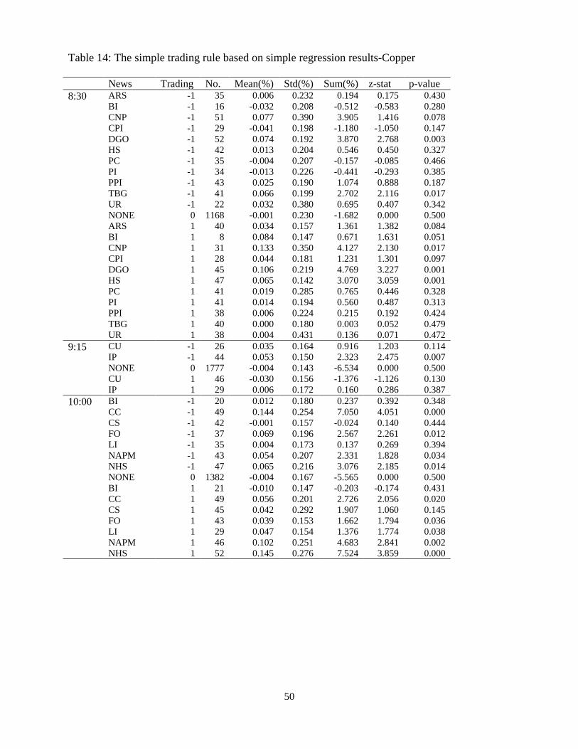
50

Table 14: The simple trading rule based on simple regression results-Copper News Trading No. Mean(%) Std(%) Sum(%) z-stat p-value 8:30 ARS -1 35 0.006 0.232 0.194 0.175 0.430

BI -1 16 -0.032 0.208 -0.512 -0.583 0.280 CNP -1 51 0.077 0.390 3.905 1.416 0.078 CPI -1 29 -0.041 0.198 -1.180 -1.050 0.147 DGO -1 52 0.074 0.192 3.870 2.768 0.003 HS -1 42 0.013 0.204 0.546 0.450 0.327 PC -1 35 -0.004 0.207 -0.157 -0.085 0.466 PI -1 34 -0.013 0.226 -0.441 -0.293 0.385 PPI -1 43 0.025 0.190 1.074 0.888 0.187 TBG -1 41 0.066 0.199 2.702 2.116 0.017 UR -1 22 0.032 0.380 0.695 0.407 0.342 NONE 0 1168 -0.001 0.230 -1.682 0.000 0.500 ARS 1 40 0.034 0.157 1.361 1.382 0.084 BI 1 8 0.084 0.147 0.671 1.631 0.051 CNP 1 31 0.133 0.350 4.127 2.130 0.017 CPI 1 28 0.044 0.181 1.231 1.301 0.097 DGO 1 45 0.106 0.219 4.769 3.227 0.001 HS 1 47 0.065 0.142 3.070 3.059 0.001 PC 1 41 0.019 0.285 0.765 0.446 0.328 PI 1 41 0.014 0.194 0.560 0.487 0.313 PPI 1 38 0.006 0.224 0.215 0.192 0.424 TBG 1 40 0.000 0.180 0.003 0.052 0.479 UR 1 38 0.004 0.431 0.136 0.071 0.472

9:15 CU -1 26 0.035 0.164 0.916 1.203 0.114 IP -1 44 0.053 0.150 2.323 2.475 0.007 NONE 0 1777 -0.004 0.143 -6.534 0.000 0.500 CU 1 46 -0.030 0.156 -1.376 -1.126 0.130 IP 1 29 0.006 0.172 0.160 0.286 0.387

10:00 BI -1 20 0.012 0.180 0.237 0.392 0.348 CC -1 49 0.144 0.254 7.050 4.051 0.000 CS -1 42 -0.001 0.157 -0.024 0.140 0.444 FO -1 37 0.069 0.196 2.567 2.261 0.012 LI -1 35 0.004 0.173 0.137 0.269 0.394 NAPM -1 43 0.054 0.207 2.331 1.828 0.034 NHS -1 47 0.065 0.216 3.076 2.185 0.014 NONE 0 1382 -0.004 0.167 -5.565 0.000 0.500 BI 1 21 -0.010 0.147 -0.203 -0.174 0.431 CC 1 49 0.056 0.201 2.726 2.056 0.020 CS 1 45 0.042 0.292 1.907 1.060 0.145 FO 1 43 0.039 0.153 1.662 1.794 0.036 LI 1 29 0.047 0.154 1.376 1.774 0.038 NAPM 1 46 0.102 0.251 4.683 2.841 0.002 NHS 1 52 0.145 0.276 7.524 3.859 0.000

51

Table 15: The simple trading rule based on simple regression results-Silver News Trading No. Mean(%) Std (%) Sum(%) z-stat p-value 8:30 ARS -1 48 0.113 0.272 5.417 2.593 0.005

BI -1 11 0.047 0.495 0.522 0.254 0.400 CNP -1 41 0.165 0.644 6.777 1.544 0.061 CPI -1 35 -0.015 0.283 -0.524 -0.507 0.306 DGO -1 46 0.016 0.316 0.758 0.148 0.441 HS -1 55 0.005 0.250 0.288 -0.124 0.451 PC -1 45 -0.085 0.297 -3.829 -2.107 0.018 PI -1 45 -0.030 0.283 -1.346 -0.922 0.178 PPI -1 45 0.005 0.333 0.216 -0.094 0.463 TBG -1 54 0.043 0.294 2.314 0.819 0.206 UR -1 42 -0.038 0.692 -1.607 -0.447 0.328 NONE 0 1401 0.010 0.265 13.333 0.000 0.500 ARS 1 47 0.050 0.318 2.350 0.862 0.194 BI 1 16 0.082 0.291 1.313 0.992 0.161 CNP 1 60 0.293 0.751 17.600 2.920 0.002 CPI 1 36 0.056 0.302 2.019 0.916 0.180 DGO 1 58 0.007 0.343 0.420 -0.050 0.480 HS 1 49 0.017 0.296 0.821 0.169 0.433 PC 1 39 0.062 0.283 2.411 1.142 0.127 PI 1 40 -0.013 0.315 -0.512 -0.443 0.329 PPI 1 54 0.079 0.304 4.273 1.661 0.048 TBG 1 47 0.094 0.363 4.416 1.582 0.057 UR 1 28 0.257 0.680 7.209 1.928 0.027

9:15 CU -1 41 0.011 0.156 0.458 0.431 0.333 IP -1 41 0.040 0.147 1.656 1.707 0.044 NONE 0 2133 0.001 0.193 1.145 0.000 0.500 CU 1 52 -0.002 0.326 -0.113 -0.060 0.476 IP 1 50 0.002 0.322 0.106 0.035 0.486

10:00 BI -1 31 0.020 0.287 0.610 0.549 0.291 CC -1 53 0.046 0.216 2.416 1.808 0.035 CS -1 46 0.011 0.258 0.484 0.504 0.307 FO -1 55 0.070 0.210 3.839 2.735 0.003 LI -1 40 0.150 0.652 5.996 1.537 0.062 NAP -1 54 0.036 0.290 1.959 1.132 0.129 NHS -1 52 0.065 0.321 3.379 1.647 0.050 NON 0 1636 -0.009 0.214 -14.422 0.000 0.500 BI 1 28 0.003 0.207 0.092 0.308 0.379 CC 1 54 -0.001 0.235 -0.075 0.229 0.409 CS 1 54 -0.074 0.260 -3.991 -1.821 0.034 FO 1 44 0.010 0.210 0.456 0.598 0.275 LI 1 33 -0.055 0.179 -1.826 -1.474 0.070 NAP 1 48 -0.060 0.247 -2.901 -1.430 0.076 NHS 1 51 0.013 0.268 0.668 0.579 0.281

52

Table 16: Cumulative profits of trading rules Cumulative Profits (%) Time Macroeconomic News Gold Copper Silver

8:30

Advance Retail Sales 5.132 1.555 7.767 Business Inventories 1.117 0.159 1.835 Change in Nonfarm Payrolls 20.745 8.032 24.377 Consumer Price Index 0.725 0.051 1.495 Durable Goods Orders 2.795 8.639 1.178 Housing Starts 1.544 3.616 1.109 Personal Consumption 2.289 0.608 -1.418 Personal Income -0.600 0.119 -1.858 Producer Price Index 1.526 1.289 4.489 Trade Balance 6.482 2.705 6.730 Unemployment Rate 3.051 0.831 5.602

9:15 Capacity Utilization -0.586 -0.460 0.345 Industrial Production 0.376 2.483 1.762

10:00

Business Inventories 1.389 0.034 0.702 Consumer Confidence 1.566 9.776 2.341 Construction Spending 1.085 1.883 -3.507 Factory Orders 3.095 4.229 4.295 Leading Indictors 0.598 1.513 4.170 NAPM 1.466 7.014 -0.942 New Home Sales 2.331 10.600 4.047

53

Figure 1: Distribution of Macroeconomic Announcements

Number of Announcements vs. Day of the Week

Number of Announcements vs. Day of the Month

0

100

200

300

400

500

1 2 3 4 5 6

Day of the Week

Num

ber o

f Ann

ounc

emen

ts

0

20

40

60

80

100

120

140

5 10 15 20 25 30

Day of the Month

Num

ber o

f Ann

ounc

emen

ts

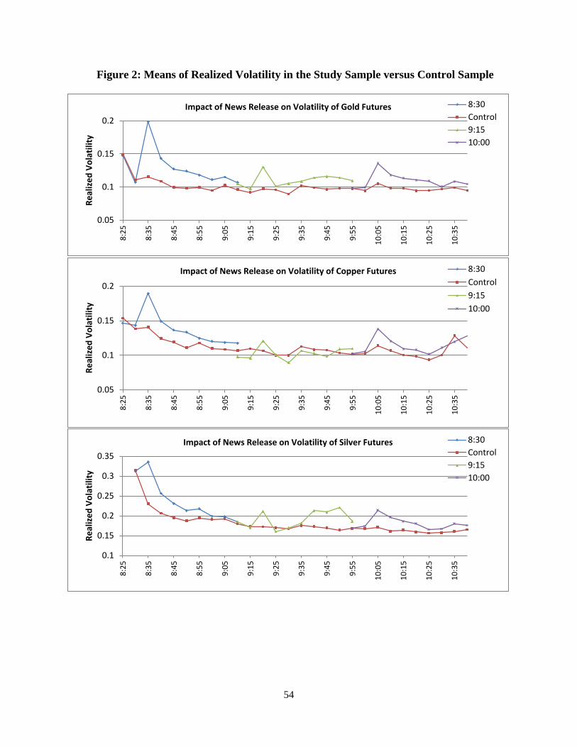
54

Figure 2: Means of Realized Volatility in the Study Sample versus Control Sample

0.05

0.1

0.15

0.28:

25

8:35

8:45

8:55

9:05

9:15

9:25

9:35

9:45

9:55

10:0

5

10:1

5

10:2

5

10:3

5

Real

ized

Vol

atili

ty

Impact of News Release on Volatility of Gold Futures 8:30Control9:1510:00

0.05

0.1

0.15

0.2

8:25

8:35

8:45

8:55

9:05

9:15

9:25

9:35

9:45

9:55

10:0

5

10:1

5

10:2

5

10:3

5

Real

ized

Vol

atili

ty

Impact of News Release on Volatility of Copper Futures 8:30Control9:1510:00

0.1

0.15

0.2

0.25

0.3

0.35

8:25

8:35

8:45

8:55

9:05

9:15

9:25

9:35

9:45

9:55

10:0

5

10:1

5

10:2

5

10:3

5

Real

ized

Vol

atili

ty

Impact of News Release on Volatility of Silver Futures 8:30Control9:1510:00

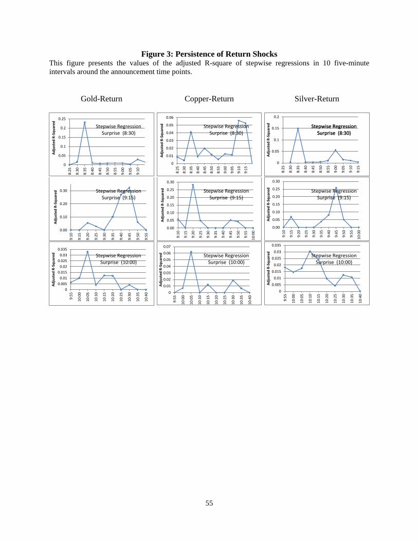
55

Figure 3: Persistence of Return Shocks This figure presents the values of the adjusted R-square of stepwise regressions in 10 five-minute intervals around the announcement time points.

Gold-Return

Copper-Return

Silver-Return

0

0.05

0.1

0.15

0.2

0.25

8:25

8:30

8:35

8:40

8:45

8:50

8:55

9:00

9:05

9:10

Adju

sted

R-S

quar

ed

Stepwise Regression Surprise (8:30)

0.00

0.10

0.20

0.30

9:10

9:15

9:20

9:25

9:30

9:35

9:40

9:45

9:50

9:55

Adju

sted

R-S

quar

ed Stepwise Regression

Surprise (9:15)

00.005

0.010.015

0.020.025

0.030.035

9:55

10:0

0

10:0

5

10:1

0

10:1

5

10:2

0

10:2

5

10:3

0

10:3

5

10:4

0

Adju

sted

R-S

quar

ed

Stepwise Regression Surprise (10:00)

0

0.01

0.02

0.03

0.04

0.05

0.06

8:25

8:30

8:35

8:40

8:45

8:50

8:55

9:00

9:05

9:10

9:15

Adju

sted

R-S

quar

ed

Stepwise Regression Surprise (8:30)

0.00

0.05

0.10

0.15

0.20

0.25

0.309:

10

9:15

9:20

9:25

9:30

9:35

9:40

9:45

9:50

9:55

10:0

0

Adju

sted

R-S

quar

ed

Stepwise Regression Surprise (9:15)

0

0.01

0.02

0.03

0.04

0.05

0.06

0.07

9:55

10:0

0

10:0

5

10:1

0

10:1

5

10:2

0

10:2

5

10:3

0

10:3

5

10:4

0

Adju

sted

R-S

quar

ed

Stepwise Regression Surprise (10:00)

0

0.05

0.1

0.15

0.2

8:25

8:30

8:35

8:40

8:45

8:50

8:55

9:00

9:05

9:10

9:15

Adju

sted

R-S

quar

ed

Stepwise Regression Surprise (8:30)

Stepwise Regression Surprise (8:30)

0.00

0.05

0.10

0.15

0.20

0.25

0.30

9:10

9:15

9:20

9:25

9:30

9:35

9:40

9:45

9:50

9:55

10:0

0

Adju

sted

R-S

quar

ed

Stepwise Regression Surprise (9:15)

0

0.005

0.01

0.015

0.02

0.025

0.03

0.035

9:55

10:0

0

10:0

5

10:1

0

10:1

5

10:2

0

10:2

5

10:3

0

10:3

5

10:4

0

Adju

sted

R-S

quar

ed

Stepwise Regression Surprise (10:00)

56

Figure 4: Persistence of Volatility Shocks This figure presents the values of the adjusted R-square of stepwise regressions in 10 five-minute intervals around the announcement time points.

Gold-Volatility

Copper-Volatility

Silver-Volatility

0

0.05

0.1

0.15

0.2

0.25

8:25

8:30

8:35

8:40

8:45

8:50

8:55

9:00

9:05

9:10

Adju

sted

R-S

quar

ed

Stepwise Regression Absolute Surprise (8:30)

0.00

0.10

0.20

0.30

0.40

0.50

9:10

9:15

9:20

9:25

9:30

9:35

9:40

9:45

9:50

9:55

10:0

010

:05

10:1

010

:15

10:2

010

:25

Adju

sted

R-S

quar

ed

Stepwise Regression Absolute Surprise (9:15)

0

0.01

0.02

0.03

0.04

0.05

0.06

0.07

9:55

10:0

0

10:0

5

10:1

0

10:1

5

10:2

0

10:2

5

10:3

0

10:3

5

10:4

0

Adju

sted

R-S

quar

ed

Stepwise Regression Absolute Surprise (10:00)

0

0.02

0.04

0.06

0.08

8:25

8:30

8:35

8:40

8:45

8:50

8:55

9:00

9:05

9:10

9:15

Adju

sted

R-S

quar

ed Stepwise Regression

Absolute Surprise (8:30)

0.00

0.05

0.10

0.15

0.20

0.259:

10

9:15

9:20

9:25

9:30

9:35

9:40

9:45

9:50

9:55

10:0

0

Adju

sted

R-S

quar

ed

Stepwise Regression Absolute Surprise (9:15)

0

0.01

0.02

0.03

0.04

0.05

9:55

10:0

0

10:0

5

10:1

0

10:1

5

10:2

0

10:2

5

10:3

0

10:3

5

10:4

0

Adju

sted

R-S

quar

ed

Stepwise Regression Absolute Surprise (10:00)

0

0.05

0.1

0.15

0.2

8:25

8:30

8:35

8:40

8:45

8:50

8:55

9:00

9:05

9:10

9:15

Adju

sted

R-S

quar

ed Stepwise Regression

Absolute Surprise (8:30)

0.00

0.10

0.20

0.30

0.40

0.50

9:10

9:15

9:20

9:25

9:30

9:35

9:40

9:45

9:50

9:55

10:0

0

Adju

sted

R-S

quar

ed

Stepwise Regression Absolute Surprise (9:15)

0

0.01

0.02

0.03

0.04

0.05

9:55

10:0

0

10:0

5

10:1

0

10:1

5

10:2

0

10:2

5

10:3

0

10:3

5

10:4

0

10:4

5

Adju

sted

R-S

quar

ed

Stepwise Regression Absolute Surprise (10:00)

57

Figure 5: Persistence of Volume Shocks This figure presents the values of the adjusted R-square of stepwise regressions in 10 five-minute intervals around the announcement time points.

Gold-Volume

Copper-Volume

Silver-Volume

0

0.05

0.1

0.15

8:25

8:30

8:35

8:40

8:45

8:50

8:55

9:00

9:05

9:10

Adju

sted

R-S

quar

ed

Stepwise Regression Absolute Surprise (8:30)

0.00

0.10

0.20

0.30

0.40

0.50

0.60

9:10

9:15

9:20

9:25

9:30

9:35

9:40

9:45

9:50

9:55

10:0

010

:05

10:1

010

:15

10:2

0

Adju

sted

R-S

quar

ed

Stepwise Regression Absolute Surprise (9:15)

0

0.02

0.04

0.06

0.08

0.1

9:55

10:0

010

:05

10:1

010

:15

10:2

010

:25

10:3

010

:35

10:4

010

:45

10:5

010

:55

11:0

0

Adju

sted

R-S

quar

ed

Stepwise Regression Absolute Surprise (10:00)

0

0.1

0.2

0.3

0.4

0.5

8:25

8:30

8:35

8:40

8:45

8:50

8:55

9:00

9:05

9:10

9:15

Adju

sted

R-S

quar

ed

Stepwise Regression Absolute Surprise (8:30)

0.00

0.10

0.20

0.30

0.40

0.50

0.609:

10

9:15

9:20

9:25

9:30

9:35

9:40

9:45

9:50

9:55

10:0

0

Adju

sted

R-S

quar

ed

Stepwise Regression Absolute Surprise (9:15)

0

0.05

0.1

0.15

0.2

9:55

10:0

0

10:0

5

10:1

0

10:1

5

10:2

0

10:2

5

10:3

0

10:3

5

10:4

0

Adju

sted

R-S

quar

ed

Stepwise Regression Absolute Surprise (10:00)

0.00

0.02

0.04

0.06

0.08

0.10

0.12

0.14

8:25

8:30

8:35

8:40

8:45

8:50

8:55

9:00

9:05

9:10

9:15

Adju

sted

R-S

quar

ed

Stepwise Regression Absolute Surprise (8:30)

0.00

0.05

0.10

0.15

0.20

0.25

0.30

9:10

9:15

9:20

9:25

9:30

9:35

9:40

9:45

9:50

9:55

10:0

0

Adju

sted

R-S

quar

ed

Stepwise Regression Absolute Surprise (9:15)

0

0.05

0.1

0.15

0.2

0.25

0.3

9:55

10:0

0

10:0

5

10:1

0

10:1

5

10:2

0

10:2

5

10:3

0

10:3

5

10:4

0

10:4

5

Adju

sted

R-S

quar

ed

Stepwise Regression AbsoluteSurprise (10:00)

58

Figure 6: Simple trading rule graph for change of nonfarm payroll

-0.1

-0.05

0

0.05

0.1

0.15

0.2

0.25

8:30 9:00 9:30 10:00 10:30 11:00 11:30 12:00 12:30 13:00 13:30

Mea

n of

5 m

inut

e ho

ldin

g re

turn

s (%

)

Time

Means of Long, Short and Notrade Based on Change of Nonfarm Payroll (GC)

Short

Long

NoTrade

-0.15

-0.1

-0.05

0

0.05

0.1

0.15

8:30 9:00 9:30 10:00 10:30 11:00 11:30 12:00 12:30 13:00 13:30

Mea

n of

5 m

inut

e ho

ldin

g re

turn

s (%

)

Time

Means of Long, Short and Notrade Based on Change of Nonfarm Payroll (HG)

Short

Long

NoTrade

-0.15

-0.1

-0.05

0

0.05

0.1

0.15

0.2

0.25

0.3

0.35

8:30 9:00 9:30 10:00 10:30 11:00 11:30 12:00 12:30 13:00 13:30

Mea

n of

5 m

inut

e ho

ldin

g re

turn

s (%

)

Time

Means of Long, Short and Notrade Based on Change of Nonfarm Payroll (SI)

Short

Long

NoTrade