Impact Resistance of Fiber-Reinforced Composites Using ...

The University of Maine The University of Maine

DigitalCommons@UMaine DigitalCommons@UMaine

Electronic Theses and Dissertations Fogler Library

Spring 5-1-2020

Impact Resistance of Fiber-Reinforced Composites Using Impact Resistance of Fiber-Reinforced Composites Using

Computational Simulations Computational Simulations

Maitham Alabbad [email protected]

Follow this and additional works at: https://digitalcommons.library.umaine.edu/etd

Part of the Engineering Mechanics Commons, Mechanical Engineering Commons, Mechanics of

Materials Commons, and the Structural Materials Commons

Recommended Citation Recommended Citation Alabbad, Maitham, "Impact Resistance of Fiber-Reinforced Composites Using Computational Simulations" (2020). Electronic Theses and Dissertations. 3174. https://digitalcommons.library.umaine.edu/etd/3174

This Open-Access Thesis is brought to you for free and open access by DigitalCommons@UMaine. It has been accepted for inclusion in Electronic Theses and Dissertations by an authorized administrator of DigitalCommons@UMaine. For more information, please contact [email protected].

https://digitalcommons.library.umaine.edu/

https://digitalcommons.library.umaine.edu/etd

https://digitalcommons.library.umaine.edu/fogler

https://digitalcommons.library.umaine.edu/etd?utm_source=digitalcommons.library.umaine.edu%2Fetd%2F3174&utm_medium=PDF&utm_campaign=PDFCoverPages

http://network.bepress.com/hgg/discipline/280?utm_source=digitalcommons.library.umaine.edu%2Fetd%2F3174&utm_medium=PDF&utm_campaign=PDFCoverPages





https://digitalcommons.library.umaine.edu/etd/3174?utm_source=digitalcommons.library.umaine.edu%2Fetd%2F3174&utm_medium=PDF&utm_campaign=PDFCoverPages

mailto:[email protected]

IMPACT RESISTANCE OF FIBER-REINFORCED COMPOSITES USING

COMPUTATIONAL SIMULATIONS

By

Maitham Alabbad

B.S. in Mechanical Engineering University of Maine, 2017

A THESIS

Submitted in Partial Fulfillment of the

Requirements for the Degree of

Master of Science

(in Mechanical Engineering)

The Graduate School

The University of Maine

May 2020

Advisory Committee:

Dr. Senthil S. Vel, Arthur O. Willey Professor of Mechanical Engineering, Co-Advisor

Dr. Roberto A. Lopez-Anido, PE, Professor of Civil Engineering, Co-Advisor

Dr. Zhihe Jin, Professor of Mechanical Engineering

IMPACT RESISTANCE OF FIBER-REINFORCED COMPOSITES USING

COMPUTATIONAL SIMULATIONS

By Maitham Alabbad

Thesis Co-Advisors: Dr. Senthil Vel and Dr. Roberto Lopez-Anido

An Abstract of the Thesis Presented

in Partial Fulfillment of the Requirements for the Degree of Master of Science (in Mechanical Engineering)

May 2020

Composite materials are widely used in aerospace, automotive and wind power industries due

to their high strength-to-weight and stiffness-to-weight ratios and their improved mechanical

properties compared to metals. The damage resistance of composite materials due to low

velocity impact depends on fiber breakage, matrix cracking and delamination between the

interfaces. In this research, a numerical investigation of low velocity impact response of a

multidirectional symmetric carbon-epoxy composite laminate is carried out and presented. Two

different finite element models are developed for composite laminates made of non-crimp fabric

to investigate their behavior under different levels of impact energy. In the first approach, a finite

element homogeneous ply model is generated wherein the heterogeneous plies are replaced by

equivalent homogeneous anisotropic plies. In the second approach, a finite element mesoscale

model that captures the individual constituents of the composite (i.e., the tows and matrix) has

been developed. Different failure criteria have been presented in the literature to predict the

damage modes of the composites during and after impact events. The 3D Hashin failure criteria

is implemented to predict the intralaminar failure and the surface-based cohesive behavior is

implemented to capture the delamination between the plies. Following the low velocity impact

investigation, the finite element models are subjected to axial compression to investigate the

compressive residual strength after impact, which is a measure of damage tolerance. The

numerical predictions, the low velocity impact response as well as the compressive residual

strength after impact, are validated with experimental data. The homogeneous ply laminate

impacted up to 50 J is seen to be capable of predicting the impact response as well as the

compressive residual strength after impact.

ii

ACKNOWLEDGEMENTS

I would like to thank my co-advisors, Dr. Senthil Vel and Dr. Roberto Lopez-Anido for their

support, feedback and guidance for the past two years. Also, I would like to acknowledge my

committee member, Dr. Zhihe Jin for his help in my undergraduate and graduate career through

teaching valuable coursework and technical knowledge.

I would like to thank my family and friends for their support and encouragement to make this

happen. I would like also to extend my thanks to Justin McDermott for his feedback and sharing

his experimental data with me. Finally, I gratefully acknowledge the Department of Mechanical

Engineering and my co-advisors for the financial support for this research work.

iii

TABLE OF CONTENTS

ACKNOWLEDGEMENTS ....................................................................................................................ii

TABLE OF CONTENTS....................................................................................................................... iii

LIST OF FIGURES ............................................................................................................................. vii

LIST OF TABLES ................................................................................................................................ xi

Chapter 1 Introduction ................................................................................................................... 1

1.1 Background ........................................................................................................................... 1

1.2 Literature review ................................................................................................................... 3

1.3 Approach ............................................................................................................................... 8

1.4 Contributions ...................................................................................................................... 10

1.5 Thesis outline ...................................................................................................................... 11

Chapter 2 Modeling of Non-Crimp Fabric Composites ................................................................. 12

2.1 Introduction ........................................................................................................................ 12

2.2 Unit Cell Modeling .............................................................................................................. 13

2.2.1 Generation of Unit Cell ................................................................................................. 13

2.2.2 Voxel Mesh Technique ................................................................................................. 18

2.2.3 Boundary Conditions .................................................................................................... 21

2.2.4 Convergence Study ....................................................................................................... 22

2.3 Structural Analysis............................................................................................................... 28

iv

2.3.1 Tensile Loading Simulation ........................................................................................... 30

2.3.2 Transverse Loading Simulation ..................................................................................... 33

2.3.3 Edge Bending Simulation .............................................................................................. 35

2.3.4 Structural Analysis Conclusion ..................................................................................... 36

2.4 Modeling of the Non-Crimp Fabric Composite ................................................................... 37

2.4.1 Mesoscale Model .......................................................................................................... 37

2.4.2 Homogeneous ply model .............................................................................................. 39

2.4.3 Mesh Generation .......................................................................................................... 40

2.4.4 Experiment Comparison ............................................................................................... 41

Chapter 3 Damage Analysis during Low Velocity Impact Loading of Multidirectional Fiber-

Reinforced Laminate ..................................................................................................................... 43

3.1 Introduction ........................................................................................................................ 43

3.2 Explicit Finite Element Simulation ...................................................................................... 45

3.2.1 Impactor Modeling ....................................................................................................... 47

3.2.2 Material Definition ....................................................................................................... 47

3.2.3 Analysis Step ................................................................................................................. 51

3.2.4 Boundary Conditions and Load Applied ....................................................................... 52

3.2.5 Contact Definition ......................................................................................................... 53

3.3 Intralaminar Damage Model ............................................................................................... 54

v

3.3.1 Damage Evolution ......................................................................................................... 56

3.4 Interlaminar Damage model ............................................................................................... 58

3.4.1 Cohesive Behavior Modeling ........................................................................................ 59

3.5 ABAQUS User Subroutine ................................................................................................... 61

3.6 Validation of Material Model .............................................................................................. 64

3.6.1 Results of Model Validation ......................................................................................... 65

3.7 Impact Simulations with Damage ....................................................................................... 69

3.8 Impact Results and Discussion ............................................................................................ 69

3.8.1 Contact Force and Displacement Histories and Absorbed Energy ............................... 70

3.8.2 Impact Damage Area Prediction ................................................................................... 81

3.8.3 Conclusion .................................................................................................................... 89

Chapter 4 Predicting the Compression After Impact Performance of Multidirectional Fiber-

Reinforced Laminate ..................................................................................................................... 90

4.1 Introduction ........................................................................................................................ 90

4.2 Compression After Impact Methodology ........................................................................... 91

4.3 Stress and Strain Calculations ............................................................................................. 94

4.4 Results and Discussion ........................................................................................................ 95

4.5 Conclusions ......................................................................................................................... 98

Chapter 5 Conclusions and Future Work/Recommendations ...................................................... 99

vi

5.1 Conclusions ......................................................................................................................... 99

5.2 Future Work/Recommendations ...................................................................................... 101

REFERENCES ................................................................................................................................ 103

APPENDICES ................................................................................................................................ 107

APPENDIX A: TexGen Scripts ................................................................................................... 107

APPENDIX B: ABAQUS (VUSDFLD) Subroutine ........................................................................ 111

BIOGRAPHY OF THE AUTHOR ..................................................................................................... 120

vii

LIST OF FIGURES

Figure 2. 1 Macroscale of fiber arrays and its corresponding unit cell ........................................ 13

Figure 2. 2 Microstructure image of the NCF specimen ............................................................... 15

Figure 2. 3 Unit cell and tow cross section ................................................................................... 15

Figure 2.4 TexGen Modeling flow chart........................................................................................ 16

Figure 2.5 Unit-cell model generated in TexGen .......................................................................... 17

Figure 2.6 Unit cell with conformal mesh technique.................................................................... 20

Figure 2.7 Tow cross section and unit cell model generated in TexGen with voxel mesh

technique ...................................................................................................................................... 21

Figure 2.8 Plot of E1 and G12 versus the number of voxels in Y direction with Z voxels

is held fixed to 12 voxels ............................................................................................................... 25






is fixed to 30 voxels ....................................................................................................................... 27

Figure 2.12 Tensile simulation load and boundary conditions ..................................................... 30

Figure 2.13 Transverse loads and boundary conditions for b) concentrated load and c)

distributed load ............................................................................................................................. 34

Figure 2.14 Edge Bending simulation load and boundary conditions .......................................... 35

viii

Figure 2.15 A mesoscale model generated in TexGen with the tows oriented 45o. .................... 39

Figure 3. 1 Results of tensile loading of the NCF composites: (a) load orientation 0o

(b) load orientation 45o (c) load orientation 90o .......................................................................... 50

Figure 3. 2 The boundary conditions applied on the composite laminate for the impact

simulation ..................................................................................................................................... 52

Figure 3. 3 Impactor's boundary conditions and load used for the impact simulations .............. 53

Figure 3. 4 Damage variable value di as a function of the failure indicator fi using the

exponential damage evolution law with Dmax = 0.8 evaluated at various values of

the material parameter m ............................................................................................................ 57

Figure 3. 5 Plot of the BK criterion with varying the value of the cohesive property

parameter ..................................................................................................................................... 61

Figure 3. 6 Flowchart of the implementation of the progressive damage model

corresponding to the user subroutine .......................................................................................... 63

Figure 3. 7 Boundary conditions and loads of single element simulations:

a) Fiber direction. b) Transverse direction. c) Shear direction. .................................................... 64

Figure 3. 8 Boundary conditions and loads of coupon simulations: a) Fiber direction.

b) Transverse direction. c) Shear direction. .................................................................................. 65

Figure 3. 9 Results of single element test loaded in (a) fiber direction (b) transverse

direction and (c) shear direction ................................................................................................... 66

Figure 3. 10 Results of coupon plate test loaded in (a) fiber direction (b) transverse

direction and (c) shear direction ................................................................................................... 68

Figure 3. 11 Numerical results for the homogeneous laminate impacted at 30 J impact:

(a) force-time (b) force-displacement and (c) deflection-time curves ......................................... 71

ix

Figure 3. 12 Out of plane displacement of the homogeneous ply model: (a) plot of the

transverse displacement of the top and bottom surfaces against the X-coordinate,

(b) X-Y plane contour plot of the top surface and (c) X-Z plane contour plot. ............................. 72

Figure 3. 13 Numerical results for the mesoscale laminate impacted at 30 J impact:

(a) force-time, (b) force-displacement and (c) deflection-time curves ........................................ 74

Figure 3. 14 Absorbed energy vs. time curves for low impact energy, 30 J ................................. 76

Figure 3. 15 Numerical results for homogeneous ply models impacted at 50 J impact:


Figure 3. 16 Numerical results for homogeneous ply model impacted at 60 J impact:


Figure 3. 17 Absorbed energies vs. time curves for high impact energy (a) 50 J impact

and (b) 60 J impact ........................................................................................................................ 81

Figure 3. 18 Predicted damage envelope compared with experimental C-scan for

laminates impacted at (a) 30 J, (b) 50 J and (c) 60 J ..................................................................... 83

Figure 3. 19 Plot of the damage area vs. incident impact energy ................................................ 84

Figure 3. 20 The predicted damage extent in each ply for the 30 J impact ................................. 85

Figure 3. 21 Predicted through thickness damage contour for different damage modes

for 30 J impact ............................................................................................................................... 86

Figure 3. 22 Predicted damage contour of the laminate impacted at 50 J .................................. 86

Figure 3. 23 Predicted damage contour of the laminate impacted at 60 J .................................. 87

Figure 3. 24 The progressive damage growth of a homogeneous ply model impacted

at 30J: (a) force-time curve, (b) fiber damage growth and (c) matrix damage growth ............... 88

x

Figure 4. 1 A schematic of ABAQUS analysis steps ....................................................................... 92

Figure 4. 2 Virtual CAI test setup of the FE model ........................................................................ 94

Figure 4. 3 Compressive stress-strain responses for undamaged homogenous model and

mesoscale model .......................................................................................................................... 97

Figure 4. 4 Compressive stress-strain responses for 30 J CAI test of homogeneous ply

model ............................................................................................................................................ 97

xi

LIST OF TABLES

Table 2. 1 The tow parameters used for the unit-cell .................................................................. 15

Table 2.2 IM7 carbon fiber properties and fiber volume fraction Vf comparison. ....................... 18

Table 2.3 Impregnated tow elastic properties ............................................................................. 23

Table 2. 4 Isotropic epoxy matrix properties (PR-520) ................................................................. 23

Table 2.5 Comparison of FE effective properties and Mori-Tanaka approach ............................. 28

Table 2.6 Number of elements generated for lamina and laminate analysis .............................. 29

Table 2.7 Result for a lamina under tensile loading for tow oriented at 0 deg. .......................... 31

Table 2.8 Result for a lamina under tensile loading for tow oriented at 45 deg. ........................ 31

Table 2.9 Result for a laminate under tensile loading for layup of [± 45o]s ................................. 32

Table 2.10 Result for a laminate under tensile loading for layup of [0o/90o]s ............................. 32

Table 2.11 Flexural response of [± 45]s laminate of concentrated force of 0.001 N ................... 34

Table 2.12 Flexural response of [± 45]s laminate of distributed load of 0.01 Pa ......................... 34

Table 2.13 Laminate result of edge bending simulation for layup of [± 45]s ............................... 35

Table 2.14 The laminate schedule [-45/45/0/90/0/±45/03/90/45]s of the non-crimp fabric ..... 38

Table 2. 15 Number of elements generated for the mesoscale and homogeneous ply

models ........................................................................................................................................... 40

Table 2.16 Experiment and prediction comparison of laminate moduli ...................................... 42

Table 3. 1 Uni-ply material strength properties ........................................................................... 48

xii

Table 3. 2 Summary of tensile test results .................................................................................... 51

Table 3. 3 Properties degradation rule ......................................................................................... 58

Table 3. 4 Cohesive parameter used in this study ........................................................................ 61

Table 3. 5 Impact parameters used in simulations ....................................................................... 69

Table 3. 6 Summary of the peak force, maximum deflection and absorbed energy for the

low impact energy ........................................................................................................................ 75

Table 3. 7 Summary of the peak force, maximum deflection and absorbed energy for high

impact energy ............................................................................................................................... 80

Table 4. 1 Results summary of CAI................................................................................................ 98

1

Chapter 1 Introduction

This thesis presents an investigation of carbon fiber-reinforced composites subjected to low

velocity impact loading and compression after impact (CAI) using computational simulations. An

experimental investigation was previously carried out at the University of Maine’s Advanced

Structure and Composites Center to analyze the damage resistance and tolerance of 3D woven

composites and 2D non-crimp fabric (NCF) composites (McDermott, 2019). The primary objective

of this thesis is to assess the damage resistance and tolerance of the NCF composites using

computational simulations. This research is carried out to support the usage of composites for

industrial applications and expand the knowledge of the mechanical behavior of composites

using numerical tools. In this study, finite element models of NCF composite are developed to

analyze their behavior under low velocity impact loading. Different damage models are used to

determine the effect of impact loading and predict the compressive residual strength of the

composite after impact. A finite element analysis is performed using ABAQUS to assess the extent

of damage and the compressive residual strength of the laminated composites. The

computational results are validated with the experimental results presented by McDermott

(2019).

1.1 Background

A composite material is formed by a combination of two or more materials to form a new

material. The most common composites are those made from fibers and held together in a binder

(Barbero, 2011, p.1). Composite material includes a very wide selection of the available materials,

2

such as fiber-reinforced polymers, metal matrix composites, ceramic matrix composites and

reinforced concrete.

Carbon fiber-reinforced composites have been widely used in industrial applications. Many

factors that influence the use of composites such as the weight reduction, high stiffness and

strength, resistance to fatigue damage and corrosion resistance. These factors enhance the use

of composites in some applications, most frequently in aerospace and transportation industries.

Composite structures subjected to different types of loading can reduce the strength of the

structures significantly. Impact loading is one of the most concerning loading in composite

structures. Impact due to tool drops or flying debris on a runway can introduce significant

damage in composite structures. Some damage in composite structures are internal and cannot

be detected by visual inspection in which this damage grows under load and can significantly

reduce the load carrying capacity of the structure (Abrate et al., 2011). Damage in composite

structure has been investigated experimentally and numerically. The finite element method plays

an important role in the industry to develop numerical tools, which could help to improve the

performance of composite structures. Numerical modelling makes it possible to accurately

generate the laminated composite models and simulate the mechanical behavior of composites

under different types of tests such as impact loading. This thesis presents a prediction of the

mechanical behavior of carbon fiber-reinforced composite subjected to impact loading as well as

predict the compressive residual strength of the laminated composite after impact. During the

impact process, the composite absorbs the impact energy in the form of various damage modes,

such as fiber breakage, matrix cracking and delamination. In order to enhance the impact

3

resistance and damage tolerance of the composite materials, various damage modes during the

impact need to be investigated using failure criteria that predict intralaminar failure (such as fiber

and matrix failure) as well as interlaminar failure (such as delamination).

1.2 Literature review

In many industries, the application of fiber reinforced composite materials has seen a rapid

growth in structural applications, especially in the aerospace industry in the past few decades.

Composite materials are used in the aircraft industry in the mid-1960s and early 1970s. The

military was the first users of composite material where it was applied on the F-14 and F-15

fighter aircraft (Safri et al., 2014). Fiber reinforced composite materials allow for numerous direct

and indirect benefits over traditional metals and metallic alloys, which generally results in lighter

weight structures. Additionally, fiber reinforced composite materials have a better fatigue

performance and resistance to corrosion compared to metals. Fiber reinforced composite

materials are naturally brittle and generally display a linear-elastic response up to failure without

any plastic deformation (Dogan et al., 2012).

Composite structures might experience structural failure and damage due to void in the

microstructure of the material, existence of a notch and corrosion of the material (Findlay et al.,

2002). Composites in structural applications or aircraft structure are exposed to many kinds of

impact loading during the process of manufacturing as well as in service (Hirai et al., 1998).

Impacts are considered one of the dangerous and unsafe types of loads because it affects the

performance of the composite laminates. It can be categorized as a low velocity impact,

intermediate impact and high velocity impact (Naik et al., 2004). The low velocity impact occurs

4

at a velocity below 10 m/s, intermediate impact occurs between 10 m/s and 50 m/s and high

impact occurs in the range of velocity from 50 m/s to 1000 m/s (Vaidya et al., 2011). For low

velocity impact, this event occurs mostly in service of during maintenance activities (Mathivanan

et al., 2010). While high velocity impact events occur mostly during take-off, flight and landing of

the aircraft. In addition, bird strikes are one of the major causes of high velocity impact due to

high probability of occurrence (Pernas-Sanchez et al., 2012). When a bird strikes an aircraft, the

relative velocities between the two bodies are so high that the material of the aircraft could

undergo instant failure (Mathivanan et al., 2010). Damage types/modes that might occur in

composite laminates due to impact are intralaminar failure such as matrix failure and fiber failure

and interlaminar failure or delamination (Zumpano et al., 2008). Matrix failure usually takes the

form of matrix cracking and it happens due to the transverse low velocity impact (Vaidya et al.,

2011). Matrix cracking is the first type of damage caused by impact and usually occurs parallel to

the fibers due to tension, compression and shearing (Sjoblom et al., 1988). However,

delamination is the most critical damage mechanism in composites due to impact. Delamination

occurs between the plies in the laminated composite (Prichard et al., 1990). Delamination or

separation between the plies happens due to bending stiffness difference between adjacent

plies, whereas fiber failure occurs due to high stress field and indentation effects. Fiber damage

usually exists after matrix cracking and delamination in the composite. The fiber damage is mostly

found just below the impactor as well as in the back face/surface due to high bending stress

(Vaidya et al., 2011).

Damage modes are commonly dependent on several parameters such as type of load applied,

model geometry, constituent material, laminate layup, impact velocity and location of the impact

5

(Carruthers et al., 1998 and Hull et al., 1991). The location of the impact region is an important

factor to understand the damage of the impact. A study conducted in the past few years (Breen

et al., 2006) shows that the damage formation and levels of strength reduction are different for

central and edge impacts. Edge impact is found to cause a greater reduction in compressive

strength while a central impact causes more tensile strength reduction. Likewise, the impact

velocity plays an important factor in the type of damage and the damaged area. Comparing the

low velocity impact with high velocity impact for the same impact energy, it was found that the

energy absorbed during low velocity impact was about 40 % lower than that of the high velocity

impact. In addition, the damage area of the low velocity impact was observed to be about 20 –

30 % smaller than the high velocity impact, and the damage area increased as the mass decreased

for high velocity impacts (Zumpano et al., 2008).

Impact situations can be simulated by performing drop weight impact simulations using a finite

element package software such as LS-DYNA and ABAQUS. A drop weight impact allows the

simulation of a wide variety of real-world impact situations and collect detailed performance data

to improve the performance of composite structures (Mathivanan et al., 2010). For modeling

purposes, a failure criterion is required to simulate damage and identify the damage mode such

as fiber or matrix failure. For intralaminar failure, some failure criteria are general which do not

have the capability to detect the failure modes such as Tsai-Wu criterion, Tsai-Hill criterion and

Azzi-Tsai-Hill criterion. Various other failure criteria have been proposed in the literature such as

Hashin and Rotem failure criteria (1973), Hashin failure criteria (1980) and Puck failure criteria

(2002). Hashin and Rotem and Hashin proposed a quadratic failure criterion in the form of

material strengths, where each branch of the criteria represents a failure mode.

6

Several researchers have used the 3D Hashin failure criteria successfully to predict the

intralaminar damage in fiber reinforced composite under low velocity impact (Megat-Yosoff et

al., 2019). Guo et al. (2013) used 3D Hashin failure criteria and exponential damage evolution

function to avoid a sudden decrease in the stiffness which may cause stiffness matrix

singularities. In addition, Maio et al. (2013) used the 3D Hashin failure criteria for intralaminar

failure initiation and exponential law proposed by Matzenmiller et al. (1995) for damage

evolution. The proposed damage model predicted delamination in a form of peanut shape and

size, aligned along the fiber direction. Zhang et al. (2015) used the three-dimensional failure

criteria proposed by Hashin and Hou et al. (2000) to predict failure in braided composites.

As previously mentioned, interlaminar damage failure or delamination is the most critical and an

important failure mode in composite materials under impact loading. Cohesive zone modeling is

the most widely used delamination modeling approach in which the interface is modeled

independently, and it does not require the knowledge of the crack position. In cohesive zone

modeling, both damage initiation and damage propagation are modeled separately. The failure

criteria in terms of interface stresses are used to predict delamination initiation, whereas the

fracture mechanics-based approach is used to predict delamination evolution (Megat-Yosoff et

al., 2019). However, Zhang et al. (2015), Topac et al. (2017) and Abir et al. (2017) used the surface-

based cohesive behavior to implement delamination between the plies under the assumption of

zero thickness zone of the cohesive zone. This modeling scheme is based on master/slave

surfaces, which follows bilinear traction separation or displacement law and it is computationally

efficient.

7

Damage tolerance is defined as the capability of a structure to continue performing their

intended functions with some tolerable level of damage (Abir et al., 2017). In composites,

damage tolerance is determined by measuring the residual strength of the composite structure.

The common approach to perform damage tolerance analysis is to carry out an impact test

followed by a CAI test to obtain the residual strength of the structure. There has not been too

much research carried out on compression after impact tests using computational simulations.

Abir et al. (2017) developed a finite element (FE) model to perform low velocity impact followed

by CAI test. The author implemented the maximum stress and Tsai Wu failure criteria for damage

initiation. It was observed that failure under CAI was due to local buckling and delamination

growth. Also, the important parameters that affect the residual strength of composites were the

Mode-II interlaminar fracture toughness and fiber compressive fracture toughness. Increase in

the Mode-II interlaminar fracture toughness reduces delamination size and increases damage

tolerance. Gonzalaz et al. (2012) performed low velocity impact and CAI simulations using

interlaminar and intralaminar damage models. The FE model predicted the compressive strength

after impact and compared it with an experiment where there is about 20% error between

simulation and experiment data. Waas et al. (2018) developed continuum shell-based FE models

to simulate the response of composite structure under impact loading the compression after

impact loading. The FE models predicted the compressive strength after impact within 7.2% in

some cases while others ranged up to 14.4%.

8

1.3 Approach

In this study, two approaches are considered to develop the finite element models of composites

and investigate their behavior under low velocity impact loading. The first approach is to develop

a homogeneous ply model as a plate where the material of the plate is considered to be

equivalent throughout the plate; therefore, there is no distinction between its constituents.

Second approach is to develop a mesoscale model as a plate which consists of tows geometries

as well as matrix geometries where the constituents of the plate are considered as different parts.

The orientation of the plies for the both models vary from layer to layer.

In the first investigation of this study, the modeling of mesoscale composites is presented. The

mesoscale finite element models are generated using TexGen software, which is an open source

software for modeling the geometry of composite structures such as woven and non-woven

composites. The mesoscale parameters, such as the tow height, tow spacing, tow width and ply

thickness, for the modeling purposes are approximated through experimental examination.

Then, unit cell models are generated using TexGen to predict the effective elastic properties

(homogenized properties) and to determine the appropriate mesh size for the mesoscale models.

In the second investigation, preliminary finite element analysis is performed using mesoscale

models and homogeneous ply models to examine the structural response of both models

subjected to different types of loads and compare them to each other. The structural analysis is

performed within the finite element analysis package ABAQUS. The structural response of the

mesoscale and homogeneous ply models is analyzed by performing static simulations of tensile

loading and flexural loading. The reason for performing the structural analysis is to ensure that

9

both models give the same structural response under certain types of static loadings before

moving to more complicated problems such as dynamic loadings.

In the next investigation, the modeling technique for the NCF laminated composites is presented.

The NCF laminated composites are used for the low velocity impact and CAI simulations. A finite

element homogeneous ply model and a finite element mesoscale model are developed to

investigate their mechanical behavior under impact loading. The homogeneous ply model is

generated within ABAQUS while the mesoscale plies are generated using TexGen. The mesoscale

plies are imported into ABAQUS for further assembly. In this study, all the parts/models are

generated with the use of continuum/solid elements. Solid elements have three translational

degrees of freedom for each node. Since this research is carried out to study the behavior of

composites subjected to impact loading, the transverse response or the through thickness

response is important to predict more accurate results. The solid elements are capable of

predicting the transverse response more accurately compared to other element types such as

shell elements. The disadvantage of solid elements is that it requires more elements compared

to shell elements to produce results with high accuracy.

In the next investigation, the mechanical behavior of the NCF laminated composites is

investigated under low velocity impact loading in ABAQUS. There are two models that are

analyzed under impact loading. The NCF laminates used in this investigation are the mesoscale

model and the homogeneous ply model. The NCF laminates are impacted with different energy

levels to examine the damage accumulation of the models. The 3D Hashin failure criteria and the

exponential damage evolution law are used in this study to evaluate the intralaminar damage

10

during impact. Additionally, the interlaminar damage is evaluated through the use of the

quadratic stress criterion and the Benzeggagh-Kenane (BK) mixed mode fracture law based on

the fracture energy release rate method. Once the impact response is simulated for the NCF

laminates, CAI simulations are performed to predict the damage tolerance of the NCF

composites. Finally, the simulations results are validated with experimental investigation.

1.4 Contributions

The aim of this research is to expand the knowledge of the mechanical behavior of carbon fiber

reinforced composites subjected to low velocity impact loading and predict the compressive

residual strength of the composites after impact. The contribution of this research falls into the

category of computational simulations. Numerical analysis tools are developed to help the

industry and institutions to improve and examine the performance of composite structures. This

tool is used to perform damage analysis of laminated composite models. In addition, a Fortran

subroutine is developed to implement the damage models of the intralaminar failure and to

evaluate the laminated composites during and after impact events.

The simulations of impact and CAI of the laminated composite models are investigated using the

FE package ABAQUS. Most of the literature consider only a homogeneous ply model to examine

the mechanical behavior of the laminates under impact loading. In this study, a mesoscale model

is considered as well to provide a more detailed description of the damage from the impact event.

The impact response of the mesoscale model is predicted and compared to the response of the

homogeneous ply model and both models are validated with experimental data.

11

1.5 Thesis outline

This thesis is organized as follows, the second chapter focuses on the modeling technique used

in this study and preliminary finite element analysis. The third chapter presents the details of

impact simulations modeling and the mechanical behavior response of the NCF laminated

composite models under impact loading. The fourth chapter details the modeling of CAI

simulations and the response of the NCF laminated composites. Conclusions and

recommendations are summarized in the fifth chapter.

12

Chapter 2 Modeling of Non-Crimp Fabric Composites

2.1 Introduction

The intention of this study is to investigate the behavior of composite laminates under impact

loading and compression after impact (CAI). The composite laminates studied in this thesis are a

multidirectional fiber-reinforced composite and consist of 24 layers. An important part of the

modeling purposes is the prediction of the effective elastic properties through a homogenization

process using unit cell finite element models. The unit cell models can be defined as the smallest

material volume element for which the macroscopic model is sufficient to represent the whole

model. The unit cell model can provide sufficient accuracy of representing the material’s larger

scale (Omairey et al., 2019). Figure 2.1 illustrates a schematic of fiber arrays and its corresponding

unit cell. A convergence study is carried out using unit cell models to determine the homogenized

elastic properties and the appropriate mesh size. Additionally, a preliminary finite element

analysis is performed to study the structural response of a lamina as well as laminates under

plane tensile and flexural loading. A mesoscale finite element model and homogeneous finite

element model are developed for the structural analysis. The mesoscale model consists of tows

geometries and matrix geometries whereas the homogeneous ply model is just a plate with using

the smeared elastic properties. Both models are used to investigate a lamina as well as laminate

plates.

The modeling of the unit cell, convergence study and structural analysis are discussed in detail in

this chapter. In addition, the generation of the composite laminate models for the impact and

13

CAI simulations are discussed as well. The finite element modeling technique and the modeling

assumptions are presented in detail along with the modeling software used.

Figure 2. 1 Macroscale of fiber arrays and its corresponding unit cell

2.2 Unit Cell Modeling

Each lamina consists of multiple in-plane tows that are embedded in a matrix. The properties of

a lamina are predicted through the use of unit cell models. The unit cell model represents the

microstructure of a single ply of unidirectional composites as shown in Figure 2.1. The unit cell is

a rectangular shape with a single tow through the thickness. The procedure of predicting the

elastic properties is called a homogenization process. The effective properties predicted, which

depend on the fiber and matrix properties as well as the fiber volume fraction and tow geometry,

are referred to as the homogenized or smeared properties.

2.2.1 Generation of Unit Cell

A non-crimp fabric (NCF) composite is investigated experimentally and presented by McDermott

(2019), and the purpose of this study is to investigate the NCF composite numerically. A

14

representative microstructure of the actual NCF composite is shown in Figure 2.2. As can be seen

from the image, the tows have an elliptical shape. Accordingly, the unit cell is modeled with a

rectangular shape consisting of one elliptical tow that is surrounded by the matrix material. The

unit cell models are constructed using TexGen software. The parameters required for modeling

the unit cell are the tow width a, tow height b, tow spacing w and ply/unit cell thickness h. The

dimensions are approximated based on the experimentally obtained microstructure image of the

actual non-crimp fabric specimen, shown in Figure 2.2. The microstructure image was analyzed

in an image processing program to approximate the needed parameters. The tow spacing is

approximated by measuring the distance between the centers of 5 adjacent tows, calculating the

average distance between the neighboring tows. The tow width is determined by measuring the

width of multiple tows and taking the average. The ply thickness is obtained by dividing the total

specimen thickness by the number of layers. Lastly, the tow height is difficult to be approximated

from the microstructure image; therefore, it was assumed to be b = 0.98*h. Figure 2.3 shows a

sketch of the cross section of the unit cell model along with the tow cross-section. The

corresponding unit cell parameters are listed in Table 2.1.

15

Figure 2. 2 A microstructure image of the NCF specimen

Figure 2. 3 Unit cell and tow cross section

Table 2. 1 The tow parameters used for the unit-cell

Unit-cell Parameters

Tow width a (mm) 2.345

Tow spacing w (mm) 2.355

Tow height b (mm) 0.1823

Ply thickness h (mm) 0.186

The unit cell models are generated through a Python script which takes as an input the unit cell

parameters. Additionally, through the use of the available built-in functions/libraries within

TexGen, the developer can specify the tow’s cross section, tow’s path, tow repetition in the X-Y

space, tow resolution and assign unit cell domain. TexGen modeling flow chart is illustrated in

16

Figure 2.4. This script can be run through TexGen and visualize the model within TexGen GUI. A

3D unit cell model generated in TexGen is shown in Figure 2.5.

Figure 2.4 TexGen modeling flow chart

17

Figure 2.5 Unit-cell model generated in TexGen

The NCF composite is fabricated using 12K fiber filament count tows. The fiber volume fraction

Vf is found to be 57.2 % experimentally by performing acid digestion test. The unit cell is modeled

using the tow’s parameters listed in Table 2.1 to predict the Vf that is approximately close to the

experimental value. TexGen has the capability to predict the total fiber volume fraction which

the fiber density and tow linear density need to be assigned to the tows in order to predict the

total Vf accurately. The fiber volume fraction Vf of the composite is the product of the fiber

volume fraction within the tows and the volume fraction of the tows:

𝑉𝑓 = 𝑉𝑓𝑡𝑜𝑤 ∗ 𝑉𝑡𝑜𝑤 (2.1)

where Vf is the composite fiber volume fraction, Vftow is the fiber volume fraction within the tow

and Vtow is the tow volume fraction . The carbon fiber properties used in this study are the IM7

carbon fiber properties from HEXCEL. The fiber density, fiber linear density and a comparison of

Vf between the experimental and predicted values are listed in Table 2.2.

18

Table 2.2 IM7 carbon fiber properties and fiber volume fraction Vf comparison.

IM7 Carbon Fiber Properties (12K)

Linear density (g/m) 0.446

Fiber Density (g/cm3) 1.78

TexGen Prediction of Vf (%)

Vftow 74.68

Vtow 76.44

Unit cell Vf 57.09

Experimental Vf 57.2

% Difference 0.19

The predicted fiber volume fraction within the tow Vftow and the tow volume fraction Vtow are

found to be 74.68 % and 76.44 % respectively. The product of the Vftow and Vtow give a unit cell

fiber volume fraction Vf to be 57.09 % with a difference of 0.19 % compared with experiment.

The predicted unit cell fiber volume fraction Vf is in good agreement with the experimental fiber

volume fraction. This small percentage difference of 0.19 % gives confidence in the unit cell

models for homogenization studies.

2.2.2 Voxel Mesh Technique

Generating a mesoscale model for a composite material can be challenging due to the complex

architecture of the tow and the surrounding resin. In this study, a voxel mesh technique is used

to mesh the geometry of the mesoscale model. However, conformal mesh technique has also

been investigated in this study. The conformal mesh technique is based on the use of tetrahedral

elements, and the use of conformal mesh technique in FE analysis results in element distortion

19

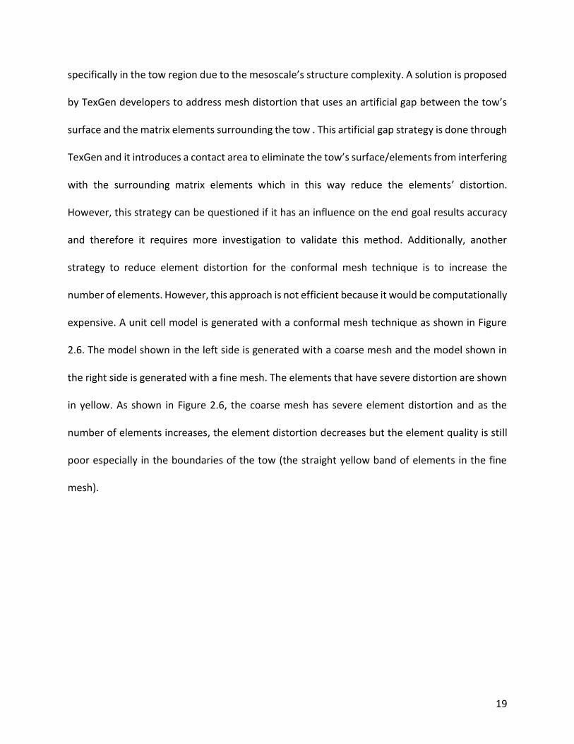
specifically in the tow region due to the mesoscale’s structure complexity. A solution is proposed

by TexGen developers to address mesh distortion that uses an artificial gap between the tow’s

surface and the matrix elements surrounding the tow . This artificial gap strategy is done through

TexGen and it introduces a contact area to eliminate the tow’s surface/elements from interfering

with the surrounding matrix elements which in this way reduce the elements’ distortion.

However, this strategy can be questioned if it has an influence on the end goal results accuracy

and therefore it requires more investigation to validate this method. Additionally, another

strategy to reduce element distortion for the conformal mesh technique is to increase the

number of elements. However, this approach is not efficient because it would be computationally

expensive. A unit cell model is generated with a conformal mesh technique as shown in Figure

2.6. The model shown in the left side is generated with a coarse mesh and the model shown in

the right side is generated with a fine mesh. The elements that have severe distortion are shown

in yellow. As shown in Figure 2.6, the coarse mesh has severe element distortion and as the

number of elements increases, the element distortion decreases but the element quality is still

poor especially in the boundaries of the tow (the straight yellow band of elements in the fine

mesh).

20

Figure 2.6 Unit cell with conformal mesh technique

The voxel mesh consists of square/rectangular hexahedral elements (C3D8, eight-node brick

element). The voxel mesh can be generated without any artificial changes in the composite

geometry. However, due to the type of element used in the voxel meshing technique, it is difficult

to capture the mesoscale model geometries very well. The mesh quality is improved by using a

large number of elements which enhances the resolution of the mesh and also captures the

mesoscale geometry (tow’s geometry) very well. The mesh for the mesoscale/unit cell model for

this study is generated in TexGen. Figure 2.7 shows a tow cross-section and FE unit cell model

with a voxel mesh technique generated within TexGen.

21

Figure 2.7 Tow cross section and unit cell model generated in TexGen with voxel mesh technique

2.2.3 Boundary Conditions

The unit cell models are constrained by implementing periodic boundary conditions. The periodic

boundary conditions can be easily applied within TexGen. The periodic boundary conditions are

implemented by creating node-to-node equation constraints in which the nodes from one side

(e.g. left side) are tied to the corresponding nodes in the other side (e.g. right side). The nodes

on opposite sides are constrained to a reference point so that the displacement of the nodes on

the opposite sides are equal to the displacement applied to the reference point. More details on

the periodic boundary conditions and its application, can be found in Li et al. (2001). The periodic

boundary conditions used in this study is to ensure the displacement in opposite sides of the unit

cell models move the same displacement and also to ensure stress continuity.

22

As mentioned previously, TexGen has the ability to apply periodic boundary conditions and

generate the mesh of the unit cell models. These unit cell models are exported as an ABAQUS

input file from TexGen along with its mesh and boundary conditions. Subsequently, the unit cell

models are imported into ABAQUS to perform a convergence study and estimate the effective

elastic properties of the composite.

2.2.4 Convergence Study

Mesh density is an important factor when it comes to accuracy of the results. Capturing the

geometry of the tows of the mesoscale/unit cell models require high mesh density. As the mesh

gets finer, the finite element analysis gets more computationally expensive. Thus, it is important

to determine the appropriate mesh size to obtain converged results within a reasonable time. To

perform the convergence study, several unit cell models are generated using TexGen as described

in section 2.2.1 with different mesh sizes to perform the convergence study. The ABAQUS input

files are exported from TexGen, and each ABAQUS file has the model information with its voxel

mesh and boundary conditions. Before post processing the input file, a small modification to the

material definition is made in ABAQUS input file to define the proper epoxy matrix properties

and impregnated tow elastic properties. The properties of the impregnated tow and epoxy matrix

are listed in Table 2.3 and 2.4. The impregnated tow elastic properties are obtained based on an

experimental investigation reported by Warren et al. (2016).

23

Table 2.3 Impregnated tow elastic properties

Tow Elastic Properties

E1t 180 GPa XT (MPa) 1810

E2t 9.45 GPa Xc (MPa) 669

E3t 9.45 GPa YT (MPa) 64.0

v12t 0.433 Yc (MPa) 174

v13t 0.433 S12 (MPa) 105

v23t 0.465 S13 (MPa) 105

G12t 6.67 GPa S23 (MPa) 105

G13t 6.67 GPa

G23t 3.23 GPa

Table 2. 4 Isotropic epoxy matrix properties (PR-520)

Matrix Properties

Em 4 GPa Tensile Strength (MPa) 82.1

vm 0.398 Compressive Strength (MPa) 128

Shear Strength (MPa) 61.4

2.2.4.1 Convergence Study Results

A total of 21-unit cell models are generated in TexGen with different mesh sizes to determine the

converged homogenized elastic properties. Three parameters, namely the voxels in the X, Y and

Z directions, need to be chosen for the mesh generation. The convergence study is divided into

four different studies. In each study, the number of voxels in the axial (X) and thickness (Z)

directions are held fixed and the number of voxels in the transverse (Y) direction is varied. This

approach is to minimize the number of voxels in Y and Z directions and still obtain converged

elastic properties. The Y and Z voxels are important parameters which they have a huge influence

on capturing the unit cell geometry (i.g. the tow’s geometry). The number of voxels in X direction

is fixed to be 5 voxels for all unit cell models since it does not influence the unit cell geometry

24

and the accuracy of the results. The number of voxels in Y direction vary from 50 to 6000 voxels

in each study. The number of voxels in Z direction are selected to be 12, 14, 20 and 30 voxels for

the first, second, third and fourth study, respectively.

The effective elastic properties are post-processed in ABAQUS by using a Python script. This script

is developed to calculate the stresses and strains from the reaction forces and the prescribed

displacements. The average composite normal stress σi is calculated by taking the reaction force

and dividing it by the surface area. Additionally, the axial strain εi is calculated by dividing the

prescribed displacement by the length of the unit cell along the corresponding direction.

Thereafter, the Young’s modulus Ei is obtained by dividing the average normal stress by the axial

strain as illustrated in equation (2.2). Furthermore, the Poisson’s ratio vij is obtained by dividing

the transverse strain by the axial strain as illustrated in equation (2.3).

𝐸𝑖 =𝜎𝑖

𝑖 (2.2)

𝑣𝑖𝑗 =− 𝑗

𝑖 (2.3)

The shear modulus Gij is obtained by dividing the shear stress τij by the shear strain ϒij in a similar

approach as the Young’s modulus. The shear modulus is calculated as illustrated in equation

(2.4).

𝐺𝑖𝑗 =𝜏𝑖𝑗

𝛾𝑖𝑗 (2.4)

The results of the FE converged effective properties are obtained for the four convergence

studies. The FE results of E1 and G12 are compared with the Mori-Tanaka approach and illustrated

25

in Figures 2.8 - 2.11. In Figure 2.8, the properties start to converge around 2000 voxels in the Y

direction whereas in Figure 2.9, the properties start to converge around 1500 voxels in the Y

direction. This indicates that as the number of voxels in Z direction increases, the smaller number

of voxels in Y direction is needed to obtain the converged effective properties. This results in a

smaller number of elements required to obtain converged results as seen in Figures 2.10 and

2.11, the properties start to converge around 950 voxels in the Y direction.

Figure 2.8 Plot of E1 and G12 versus the number of voxels in Y direction with Z voxels is held fixed to 12 voxels

4.2

4.3

4.4

4.5

4.6

4.7

4.8

4.9

5

5.1

138.2

138.6

139

139.4

139.8

140.2

140.6

141

141.4

0 1000 2000 3000 4000 5000 6000

G1

2(G

pa)

E 1(G

Pa)

Number of Voxels in Y-direction

Convergence Study (12 voxels in z)

E1 E1 (MT) G12 G12 (MT)

26



4.2

4.3

4.4

4.5

4.6

4.7

4.8

4.9

5

5.1

138.2

138.6

139

139.4

139.8

140.2

140.6

141

141.4

0 1000 2000 3000 4000 5000 6000

G1

2(G

Pa)

E 1(G

Pa)



E1 E1 (MT) G12 G12 (MT)

4.2

4.3

4.4

4.5

4.6

4.7

4.8

4.9

5

5.1

138.2

138.6

139

139.4

139.8

140.2

140.6

141

141.4

0 1000 2000 3000 4000 5000 6000

G1

2(G

Pa)

E 1(G

Pa)



E1 E1 (MT) G12 G12 (MT)

27

Figure 2.11 Plot of E1 and G12 versus the number of voxels in Y direction with Z voxels is fixed to 30 voxels

The convergence study is used to determine the number of elements required to obtain accurate

FE results. As seen in Figure 2.11, the effective elastic properties converge around 950 voxels in

the Y-direction and the computed properties correlate well compared with the Mori-Tanaka

approach. Comparing the results presented in Figures 2.10 and 2.11, there is no significant

difference in both moduli E1 and G12. Therefore, a small number of voxels in Z direction is used,

20 voxels, since there is no significant difference to the results of using 30 voxels in Z direction. A

comparison between the converged FE elastic properties with Mori-Tanaka method is shown in

Table 2.5. overall, the FE results found to be close to the approximated properties using the Mori-

Tanaka method. The shear modulus G12 has a large percentage difference between FE approach

and Mori-Tanaka method. This is because the Mori-Tanaka method approximates the elastic

4.2

4.3

4.4

4.5

4.6

4.7

4.8

4.9

5

5.1

138.2

138.6

139

139.4

139.8

140.2

140.6

141

141.4

0 1000 2000 3000 4000 5000 6000

G1

2(G

Pa)

E 1(G

Pa)



E1 E1 (MT) G12 G12 (MT)

28

properties based on the assumption that the tow has a circular cross-section whereas in this

study the tow has more of an elliptical cross-section.

Table 2.5 Comparison of FE effective properties and Mori-Tanaka approach

Effective Properties FE Approach Mori-Tanaka Method FE and Mori-Tanaka %Difference

E1 (GPa) 139.54 138.5443 0.7161

E2 (GPa) 8.276 7.8981 4.6729

E3 (GPa) 8.2018 7.8981 3.7727

v12 0.4265 0.42501 0.3500

v13 0.4242 0.42501 0.1908

v23 0.5013 0.51708 3.0990

G12 (GPa) 4.9818 4.2289 16.3484

G13 (GPa) 4.3491 4.2289 2.8025

G23 (GPa) 2.5168 2.6031 3.3712

2.3 Structural Analysis

A preliminary finite element analysis (FEA) is performed in ABAQUS using mesoscale models and

homogeneous ply models. The mesoscale models of lamina and laminate are generated in

TexGen using the impregnated tow elastic properties and matrix properties listed in Table 2.3

and Table 2.4, respectively. Whereas the homogeneous ply models of lamina and laminate are

generated in ABAQUS using the converged FE elastic properties (homogenized properties)

presented in Table 2.5. The structure response of both models is analyzed by performing static

simulations of tensile and flexural tests.

29

Models of one ply with orientation of 0o and 45o and laminates with orientation of [±45o]s and

[0o/90o]s are developed for the structural response analysis of both mesoscale and homogeneous

ply models. The lamina and laminate dimensions used are 14.13 mm x 14.13 mm x 0.186 mm and

14.13 mm x 14.13 mm x 0.744 mm, respectively. Number of elements generated for lamina and

laminate models are listed in Table 2.6. The mesoscale model is meshed using 8-node linear brick

C3D8 and the homogeneous ply model is meshed using 8-node linear brick, reduced integration

and hourglass control C3D8R. The use of C3D8R for the mesoscale would result in some element

distortion. To eliminate the element distortion, the fully integrated element C3D8 must be used

for the mesoscale models. Fully integrated elements have four integration points compared to

the reduced integration elements which have only one integration point at the centroid of the

element. Reduced integration elements take less time to solve due to the reduced order of

integration, but it might not have the capabilities to detect strains at the integration point

accurately for the mesoscale model since there two material properties are defined, for example,

fiber and matrix material properties. Thus, fully integrated elements are required in order to

capture an accurate structure response of the mesoscale that can be comparable to the structure

response of the homogeneous ply model.

Table 2.6 Number of elements generated for lamina and laminate analysis

Lamina Models Mesoscale 2,100,000

Homogeneous 150,000

Laminate Models Mesoscale 1,920,000

Homogeneous 240,000

30

2.3.1 Tensile Loading Simulation

A lamina and laminate structure of mesoscale and homogeneous ply models are analyzed

subjected to tensile loading. For tensile loading analysis, the boundary conditions and load used

are shown in Figure 2.12. The load is applied to the models using displacement control. A

prescribed displacement is applied using kinematic coupling constraint. The kinematic coupling

constraint is very useful in this case since there are a large number of nodes. The kinematic

coupling constrains the motion of the slave nodes to the motion of a single reference point which

is the master node.

Figure 2.12 Tensile simulation load and boundary conditions

The Young’s modulus Ex and Poisson ratio vxy are calculated and compared between the

mesoscale and homogeneous ply models. The results of the Young’s modulus and Poisson’s ratio

are calculated using the average stress and strain as illustrated in equation (2.5). The average

31

values of stress and strain are calculated by taking the summation of stress and strain of all

elements and dividing them by the total number of elements.

𝐸𝑥 =��𝑥

𝑥 𝑣𝑥𝑦 = −

𝑦

𝑥 (2.5)

where 𝜎𝑥 is the average stress in X direction, 𝜀�� is the average strain in X direction and 𝜀�� is the

average strain in Y direction. The results for a lamina with orientation of 0o and 45o under tensile

loading are presented in Tables 2.7 and 2.8, respectively.

Table 2.7 Result for a lamina under tensile loading for tow oriented at 0 deg.

Models Ex (GPa) vxy

Mesoscale 139.522 0.4274

Homogeneous 139.539 0.4265

% Difference 0.013 0.223

Table 2.8 Result for a lamina under tensile loading for tow oriented at 45 deg.

Models Ex (GPa) vxy

Mesoscale 12.4703 0.2302



32

The results for a laminate with orientation of [± 45o]s and [0o/90o]s under tensile loading are

presented in Tables 2.9 and 2.10, respectively.

Table 2.9 Result for a laminate under tensile loading for layup of [± 45o]s

Models Ex (GPa) vxy

Mesoscale 18.416 0.7207



Table 2.10 Result for a laminate under tensile loading for layup of [0o/90o]s

Models Ex (GPa) vxy

Mesoscale 75.422 0.0569



The results for tensile simulation of a lamina of mesoscale model and homogeneous ply model

are in good agreement. The percentage difference of the Young’s modulus Ex between the

mesoscale model and the homogeneous ply model of a lamina with orientation of 0o and 45o are

0.013 % and 0.576 %, respectively. Also, the percentage difference of the Poisson ratio vxy

between the mesoscale model and the homogeneous ply model of a lamina with orientation of

0o and 45o are 0.223 % and 5.995 %, respectively. However, there is a difference between the

results for the laminate models of [±45o]s and [0o/90o]s. For [±45o]s laminates, the percentage

difference of the Young’s modulus Ex and Poisson ratio vxy between mesoscale and homogeneous

ply models are 5.531 % and 3.834 %, respectively. In the case of [0o/90o]s laminates, the

33

percentage difference of the Young’s modulus Ex and Poisson ratio vxy between mesoscale and

homogeneous ply models are 1.207 % and 3.303 %, respectively. This difference is because the

geometry of the mesoscale models was not captured accurately; therefore, the results are

under/over predicted. When the tows in the mesoscale models are oriented with orientation

other than 0o, it gets very complex to capture the tows’ geometry with the use of the hexahedral

solid element that is aligned with the coordinate axes. Due to the nature of the hexahedral solid

element, some of the tow’s elements are taken as matrix elements which lead to over/under

predicting the results of the mesoscale models.

2.3.2 Transverse Loading Simulation

Mesoscale and homogeneous ply models of composite laminate are analyzed under transverse

loading. Mesoscale and homogeneous laminates, with orientation of [±45o]s, are developed to

analyze the flexural response of the composite models. Two studies are performed. In the first

study, the composite plate is analyzed under a concentrated force applied in the center of the

plate. While the second study, the composite plate is analyzed under uniform distributed load.

The composite plate is simply supported for both studies as shown in Figure 2.13(a). A

concentrated force of 0.001 N is applied in the first study whereas a uniform distributed load of

0.01 Pa is applied in the second study as illustrated in Figure 2.13 (b) and (c), respectively.

34

Figure 2.13 Transverse loads and boundary conditions for b) concentrated load and c) distributed load

The flexural response for the concentrated force and distributed load cases are summarized in

Tables 2.11 and 2.12, respectively. The maximum deflection of the composite plates is compared.

The mesoscale and homogeneous ply models correlate well in the case of the concentrated force

as well as in the case of the distributed load with a percentage difference of 0.75 % and 0.086 %,

respectively.

Table 2.11 Flexural response of [± 45]s laminate of concentrated force of 0.001 N

Mesoscale Model Homogenized Model

Deflection (mm) - 3.9949 x 10-6

mm - 3.9652 x 10-6

mm % Difference: 0.75 %

Table 2.12 Flexural response of [± 45]s laminate of distributed load of 0.01 Pa


Deflection (mm) - 4.5937 x 10-3

mm - 4.5898 x 10-3

mm % Difference: 0.086 %

35

2.3.3 Edge Bending Simulation

Mesoscale and homogeneous laminates, with orientation of [±45o]s, are developed to analyze

their response under concentrated force applied along an edge of the laminates. The composite

laminates are simply supported and a concentrated force of 0.01 N is applied along one of the

laminate edges as illustrated in Figure 2.14.

Figure 2.14 Edge Bending simulation load and boundary conditions

The structural response of the edge bending test is summarized in Table 2.13. The maximum

displacement of the mesoscale and homogeneous ply models is compared. About 6% difference

between the mesoscale and homogeneous ply models. The difference is due to the mesoscale

tow geometries were not captured very well. Due to the nature of the voxel mesh, some of the

tow’s elements are taken as matrix elements in the mesoscale model which results in larger

deflection in the mesoscale model compared to the homogenous model.

Table 2.13 Laminate result of edge bending simulation for layup of [± 45]s


Deflection (mm) - 2.84106 x 10-2 - 2.67756 x 10

-2 % Difference: 5.9 %

36

2.3.4 Structural Analysis Conclusion

A preliminary finite element analysis has been performed to study the structural response of a

composite lamina as well as laminates under tensile loading and flexural loading. A mesoscale

model and a homogeneous ply model are used for the structural analysis of the composite lamina

and laminates. For composite lamina analysis, the structural response comparison between the

mesoscale models and the homogeneous ply models is in good agreement. However, there are

discrepancies in the structural response of the composite laminates between the mesoscale and

homogeneous ply models. The difference in the laminates analysis is due to how the tows

geometries are captured in the mesoscale models. The tow elements in the [±45o]s laminate are

taken as matrix elements which results in under/over predicting the structural response of the

mesoscale model. For the [0o/90o]s laminate, there is no issue when it comes to capture the

geometry of the tows oriented at 0o, but for 90o orientation, the tows require more elements (or

voxels) in the X direction to capture the tows accurately.

Overall, based on the preliminary finite element analysis, it can be concluded that the mesoscale

finite element model and the homogeneous finite element model generate a similar structural

response. However, the mesoscale model requires a large number of elements to give a

comparable structural response to the homogeneous ply model. Therefore, both models can be

used in this study to generate the composite laminates for the impact and compression after

impact simulations.

37

2.4 Modeling of the Non-Crimp Fabric Composite

NCF composite laminates are developed to analyze their behavior under impact loading and

predict the compressive residual strength after impact. A mesoscale finite element model and a

homogeneous finite element model are developed to assess the damage resistance and

tolerance of the laminated composites. Both models are generated based on the non-crimp

fabric specimen that has been investigated experimentally by McDermott (2019). The NCF

specimen is fabricated with a multidirectional 24 plies and each ply consists of one tow through

the thickness. The NCF model is generated to be consistent with the specimen used in the

experiment. The modeling parameters for the mesoscale model such as the tow width, tow

spacing, tow height and ply thickness are obtained based on experimental investigation as

discussed in Section 2.2.1. Since the mesoscale model has tow geometries and matrix

geometries, it provides the ability to evaluate the fiber and matrix damage separately for the

impact analysis. The response of the impact and compression after impact of the mesoscale and

homogeneous ply models is used to be compared with experimental data obtained from

McDermott (2019).

2.4.1 Mesoscale Model

A finite element mesoscale model is generated to investigate the behavior of the model

subjected to impact loading and predict the compressive residual strength after impact. As

previously mentioned, the finite element mesoscale model is developed where the model

captures the individual constituents of the composite (i.e., the tows and matrix). This modeling

approach helps to evaluate the damage during impact and after impact events in more detail

38

such that a separate investigation of the fiber and matrix failure. The modeling parameters for

the mesoscale model are listed in Table 2.1. The mesoscale model is generated as a

multidirectional symmetric NCF laminate with 24 layers. The NCF laminate schedule is shown in

Table 2.14. Four plies with orientation of -45o, 45o, 0o and 90o are generated separately in TexGen

with one tow through the thickness. Each ply is generated with 64 in-plane tows and one tow

through the thickness. The four plies are imported into ABAQUS for further assembly of the

composite mesoscale laminate. The mesoscale model dimensions are 150.72 mm x 100 mm x

4.464 mm. The impregnated tow elastic properties and epoxy matrix properties used for the

mesoscale model are listed in Tables 2.3 and 2.4, respectively.

Table 2.14 The laminate schedule [-45/45/0/90/0/±45/03/90/45]s of the non-crimp fabric

Midplane

12 45

11 90

10 0

9 0

8 0

7 -45

6 45

5 0

4 90

3 0

2 45

1 -45

A Python script is developed for the mesoscale generation and processed in TexGen. As

mentioned, the plies are generated with one tow through the thickness. Four plies are developed

with different tow’s orientation 0o, 45o, -45o and 90o. For simplicity, the script generates the plies

and exports an ABAQUS input file with the ply’s information. The element type used is C3D8 solid

39

element. All four plies are imported into ABAQUS with their proper tow’s orientation and mesh.

The assembly of the mesoscale model can be done through TexGen but to implement the

interlaminar failure criteria between the plies, it is easier to assemble the model and implement

the failure criteria in ABAQUS. A sample mesoscale ply generated in TexGen with the tows

oriented 45o is shown in Figure 2.15. A Python script of the ply generation is attached in Appendix

A.

Figure 2.15 A mesoscale model generated in TexGen with the tows oriented 45o.

2.4.2 Homogeneous ply model

A finite element homogeneous ply model is developed in ABAQUS to analyze the behavior of the

model under impact loading and predict the compressive strength of the laminate after impact.

The finite element homogeneous ply model is generated wherein the heterogeneous plies are

replaced by equivalent homogeneous anisotropic plies. The plies of the homogeneous model are

created using 3D deformable solid elements. Plies with orientation of 45o, -45o, 0o and 90o are

created separately and then used to assemble the laminate based on the composite layup in

40

Table 2.14. The homogeneous ply model dimensions are 150 mm x 100 mm x 4.464 mm. The

material orientation is defined using the available tool in ABAQUS. A local coordinate system is

defined for each ply. Then, each ply is assigned a material orientation based on the local

coordinate system of the ply. The homogenized properties listed in Table 2.5 are used for this

model.

2.4.3 Mesh Generation

The composite laminates for the impact and compression after impact events are meshed using

the voxel mesh technique. The mesoscale model is meshed within TexGen. The element type

used for the mesoscale is the 8-node brick element C3D8. This element type is a general-purpose

linear brick element and it is fully integrated. However, the homogeneous ply model is meshed

within ABAQUS with fully integrated 8-node brick element C3D8. The fully integrated elements

are used for the homogeneous ply model with fewer number of elements compared to the

mesoscale model. Based upon the structural response analysis presented in Section 2.3, the

mesoscale model requires high mesh density (large number of elements) to capture the tows

geometries accurately. The total number of elements generated for the mesoscale model as well

as the homogeneous ply model is listed in Table 2.15.

Table 2. 15 Number of elements generated for the mesoscale and homogeneous ply models

Model Element Type Number of Elements

Homogeneous ply model C3D8 460,800

Mesoscale Model C3D8 1,920,000

41

2.4.4 Experiment Comparison

In this section, the homogenized properties are validated with experimental data by predicting

the laminate Young’s modulus Ex and Ey. This validation is performed to ensure that the

homogenized properties estimate the laminate modulus close to the experimental values. The

experiment is presented in McDermott (2019). The Young’s modulus Ex and Ey are obtained

experimentally by performing tension tests. The experimental results are the average value of

seven to eight specimens. The specimens are loaded in tension in the 0o and 90o orientation. To

predict the Young’s modulus Ex and Ey, the extensional stiffness matrix [A] was computed using

the classical laminate theory. The inverse of [A], the compliance matrix [a], is calculated to predict

the Young’s modulus Ex and Ey using equation (2.6).

𝐸𝑥 =1

𝑎11𝐻 𝐸𝑦 =

1

𝑎22𝐻 (2.6)

where a11 and a22 are the extensional terms and H is the laminate thickness. Table 2.16

summarizes the results of both experimental and predicted results of the laminate moduli. As

shown in the results, there is no significant difference between the experimental and predicted

results. A 0.71 % and a 2.48 % difference for Ex and Ey, respectively. The predicted and

experimental results correlate well which demonstrate confidence in the composite laminate

model.

42

Table 2.16 Experiment and prediction comparison of laminate moduli

Vf (%)

Laminate Moduli (GPa)

Ex E

y

Experimental Predicted Diff. (%) Experimental Predicted Diff. (%)

57.2 – Expt. 57.09 –Pred.

72.2 72.511 0.71 40.7 41.72 2.48

43

Chapter 3 Damage Analysis during Low Velocity Impact Loading

of Multidirectional Fiber-Reinforced Laminate

3.1 Introduction

Unidirectional fiber-reinforced composites are being increasingly used in automobiles,

aerospace, and many other industries due to their higher structural strength, low weight and

impact tolerance compared to those of metallic parts. One of the objectives of this research is to

perform computational simulations of carbon fiber-reinforced composites subjected to low

velocity impact loading using finite element analysis. Two finite element models are developed

to analyze the behavior of composite laminates made of non-crimp fabric under impact loading.

The finite element models are developed as symmetric laminates of 24 multidirectional plies. The

first model is a homogeneous ply finite element model which is generated within the finite

element package ABAQUS. The second model is a mesoscale finite element model where its plies

are generated using textile generation software called TexGen. The mesoscale plies are imported

into ABAQUS for the mesoscale laminate assembly. The modeling details of the non-crimp fabric

models are presented in Chapter 2. The impact simulations of the homogeneous ply and

mesoscale models are setup and performed using ABAQUS/Explicit.

The 3D Hashin failure criteria is used to evaluate the intralaminar damage initiation of the

composite laminates during impact event. The Hashin failure criteria has four failure

modes/indicators. Two modes are for fiber tension and compression failure initiation and the

other two modes are for matrix tension and compression failure initiation. In addition, a damage

44

evolution law is adopted to determine the damage variables for each failure mode. These

damage variables are used to modify or degrade the elastic properties based on the induced

damage mode.

Additionally, the interlaminar failure is evaluated using a surface-based cohesive behavior. This

approach implements cohesive contact behavior between the plies to predict delamination. The

damage initiation is evaluated using the quadratic stress criterion. A damage evolution law is

implemented to describe the rate at which the cohesive stiffness is degraded once the

corresponding initiation criterion is reached. Mixed mode failure criterion based upon energies

is used for interlaminar damage propagation.

The proposed progressive intralaminar damage models are implemented in ABAQUS using a

Fortran user defined subroutine. This subroutine checks for failure initiation at every integration

point using the Hashin failure criteria and computes the damage variables using the exponential

law. It then returns the damage variables to ABAQUS using the field variable tool for material

properties assignment. A look up table is defined in ABAQUS input file to relate the field variables

to the original elastic material properties as well as the degraded material properties. The impact

results of both homogeneous ply and mesoscale models are compared with each other and

validated with experimental data. All experimental data used to validate the finite element

models presented in this chapter are obtained from McDermott (2019).

This chapter is organized as follows, Section 3.2 describes the explicit finite element simulation

algorithm, and Section 3.3 describes the intralaminar damage models. Section 3.4 summarizes

the modeling of delamination using cohesive behavior. Section 3.5 contains an outline of the

45

implementation of the Fortran user subroutine and its interaction with ABAQUS. The material

model validation using ABAQUS subroutine is summarized in Section 3.6. Sections 3.7 and 3.8

summarize the impact simulations with damage followed by the results of the impact simulations

section, respectively.

3.2 Explicit Finite Element Simulation

Impact simulations can be performed using ABAQUS/Implicit and ABAQUS/Explicit. In this thesis,

ABAQUS/Explicit is used to evaluate the finite element models under impact loading.

ABAQUS/Explicit is a finite element analysis product that is applicable to analyze many types of

problems such as short duration dynamic, nonlinear, quasi-static analyses and many more.

ABAQUS/Explicit has the ability to handle nonlinear behavior efficiently, which makes it a perfect

candidate for the present study. Some of the advantages of using ABAQUS/Explicit in this study

compared to ABAQUS/Implicit are as follows:

● It has been designed to solve highly discontinuous and high-speed dynamics problems.

● It has a robust contact algorithm that does not require additional degrees of freedom.

● It does not require large disk space for analyzing large problems.

ABAQUS/Explicit uses an explicit method that integrates through time. The explicit time

integration used is the central difference method. The equations of motion are integrated

through time. When the solver is initiated, it solves the discretized equation of motion (3.1) to

obtain the nodal acceleration for each time increment (ABAQUS, 2017).

𝑀�� = 𝑃 − 𝐼 (3.1)

46

where M is the nodal mass matrix, �� is the nodal acceleration, P is the external force applied and

I is the internal element force.

Nodal velocities are calculated using the nodal accelerations. Nodal accelerations are integrated

through time using the central difference approach. The change in velocity is calculated by

assuming that the acceleration is constant. The velocity at the middle of the current increment is

obtained using the acceleration and the velocity at the middle of the previous increment using

equation (3.2) (ABAQUS, 2017).

��|(𝑡+

∆𝑡

2)

= ��|(𝑡−

∆𝑡

2)

+∆𝑡|(𝑡+∆𝑡)+ ∆𝑡|(𝑡)

2 𝑢| (𝑡) (3.2)

Similarly, the nodal displacements are obtained by integrating the nodal velocities using equation

(3.3).

𝑢|(𝑡+∆𝑡) = 𝑢|(𝑡) + ∆𝑡|(𝑡+∆𝑡) 𝑢|(𝑡+

∆𝑡

2) (3.3)

To obtain accurate results, sufficiently small-time increments must be used to have nearly

constant accelerations. Since a small-time increment is used, a large number of increments is

required to finish the analysis. However, each increment is computationally inexpensive since the

equations are not solved at the same time. The element strain increments are computed from

the strain rate. The computed strain increment makes it possible to compute the element

stresses by applying the material constitutive relationships (ABAQUS, 2017).

47

The process described is performed for each time increment. When all the above stated steps

are applied for the current increment, the process gets repeated for the next increment by setting

a new time for the next increment (ABAQUS, 2017).

3.2.1 Impactor Modeling

The hemispherical impactor is modeled in ABAQUS as a 3D discrete rigid body. The impactor is

modeled with a diameter of 16 mm and a spherical tip shape to be consistent with the

experiment setup. It is meshed with linear quadrilateral elements of type R3D4 and linear

triangular elements of type R3D3 with a total of 11,232 elements.

3.2.2 Material Definition

The material system used for the impact simulation study is Hexcel® 12K IM7 carbon fibers and

Cycom® PR-520 toughened epoxy matrix. The mesoscale model is assigned the material

properties of the impregnated tow elastic properties listed in Table 2.3 and matrix properties

listed in Table 2.4. The material properties used for the homogeneous ply model are the effective

elastic properties listed in Table 2.5, which are found based on the convergence study presented

in Chapter 2.

The density cannot be assigned for the impactor since it is modeled as a rigid body. Instead, an

inertia is assigned to it to account for the total drop weight. For the impact simulations, the

impactor is assigned a mass corresponding to the impact energies and impact velocity.

48

Due to the lack of the material properties of the current investigated composite, the composite

material strengths are used from previous study investigated by Warren et al. (2016). Warren

used the same material system IM7/PR-520 for his study and he investigated a uni-ply panel of

IM7 carbon fiber manufactured with 24K tows and injected with PR-520 epoxy resin. The fiber

volume fraction of the panel is 61.4 %. The panel was evaluated experimentally to compute the

material properties by loading the panel in tension, compression and shear directions. The

material strengths obtained experimentally are listed in Table 3.1.

Table 3. 1 Uni-ply material strength properties

Load Symbol Strength (MPa)

Tensile strengths

XT 1750

YT 69.6

Compressive strengths

XC 665

YC 177

Shear strength S 106

Mechanical properties validation is performed using computational simulations and compared

to experimental investigation presented by McDermott (2019). The NCF model is generated in

ABAQUS to validate the material strengths properties listed in Table 3.1. The FE model is a

multidirectional NCF composite and consists of 24 layers. The layup schedule of the NCF

49

composite is shown in Table 2.14. The FE model is evaluated in tensile loading oriented parallel

to, perpendicular to and biased to (oriented at 45o) the fiber direction. For tensile testing, the FE

model is generated with 3D solid elements and dimensions of 100 mm x 25 mm x 4.464 mm. It is

meshed with C3D8 elements and assigned the homogenized properties listed in Table 2.5. The

experiment is carried out with ASTM D3039. Seven to eight specimens were characterized

experimentally at each load orientation 0o, 45o and 90o. The specimens tested experimentally of

IM7 carbon fiber are manufactured with 12K tows and injected with PR-520 epoxy resin. The

results of the tensile loading are presented in Figures 3.1a-c which shows the correlation between

the finite element simulations and experimental results. The computational model predicted the

mechanical behavior of the tensile tests very well. A summary of the tensile tests results is

presented in Table 3.2. The experimental results presented in Table 3.2 are the average value of

multiple specimens. It can be concluded that the tensile strength properties presented in Table

3.1 are valid to be used in this study with knowing that the tow size is different between Warren’s

work and this current study. The other strength properties for the compression and shear are

assumed to be valid as well.

50

Figure 3. 1 Results of tensile loading of the NCF composites: (a) load orientation 0o (b) load orientation 45o (c) load orientation

90o

0

200

400

600

800

1000

1200

0 0.5 1 1.5 2

Ten

sile

Str

ess

(MP

a)

Tensile Strain (%)

Stress-Strain Curves for NCF Composite (orientation: 0)

Specimen 1

Specimen 2

Specimen 3

Specimen 4

Specimen 5

Specimen 6

Specimen 7

FEA

(a)

0

200

400

600

800

0 0.5 1 1.5 2

Ten

sile

Str

ess

(MP

a)

Tensile Strain (%)

Stress-Strain Curves for NCF Composite (orientation:45)

Specimen 1

Specimen 2

Specimen 3

Specimen 4

Specimen 5

Specimen 6

Specimen 7

FEA

(b)

0

200

400

600

800

0 0.5 1 1.5 2

Ten

sile

Str

ess

(MP

a)

Tensile Strain (%)

Stress-Strain Curves for NCF Composite (orientation: 90)

Specimen 1

Specimen 2

Specimen 3

Specimen 4

Specimen 5

Specimen 6

Specimen 7

Specimen 8

FEA

(c)

51

Table 3. 2 Summary of tensile test results

Load Orientation Ultimate Strength (MPa) Young’s Modulus (GPa)

0o

Experiment 983 72.2

FEA prediction 885 72

45o

Experiment 709 51.8

FEA prediction 626.8 51.5

90o

Experiment 566 40.7

FEA prediction 505.2 41.3

3.2.3 Analysis Step

The analysis step is created in the step module in ABAQUS, the procedure of the step is chosen

to be Dynamic Explicit with a step time in the range of 5 to 9 milliseconds for the impact

simulations. The geometric nonlinearity is toggled on in the basic tab. Automatic time

incrementation is used with the stable increment estimator is selected to be global with a time

scaling factor of 1. Since the density and the Young’s modulus are known, the critical parameter

for the stable time increment is the dimension of the smallest element. The composite laminates

are modeled to have the smallest element dimension which limits the stable time increment for

the whole model/assembly of the impact setup. Maximum time increment is kept to its default

setting, unlimited. Mass scaling is not applied for any region of the model and the linear and

quadratic bulk viscosity parameters are set to default values of 0.06 and 1.2, respectively.

52

3.2.4 Boundary Conditions and Load Applied

The boundary conditions used for the finite element laminated composite are a representation

of the experimental setup used in the impact test. The drop weight test is carried out

experimentally using Airbus Industries AITM 1-0010 standard. In order to represent the

experiment setup, the laminated composite is simply supported in the entire inner perimeter, 75

mm x 125 mm, such that the displacement component U3=0. Additionally, two constraints are

included to prevent the laminate from translating and rotating in the other directions. The

boundary conditions applied on the composite laminate for the impact simulations are shown in

Figure 3.2.

Figure 3. 2 The boundary conditions applied on the composite laminate for the impact simulation

The 16 mm hemispherical rigid impactor is modeled with a reference point at the impactor tip to

be able to apply boundary conditions and load. The impactor’s reference point is fixed in all

directions except the impact translation direction. Additionally, an impact velocity is applied to

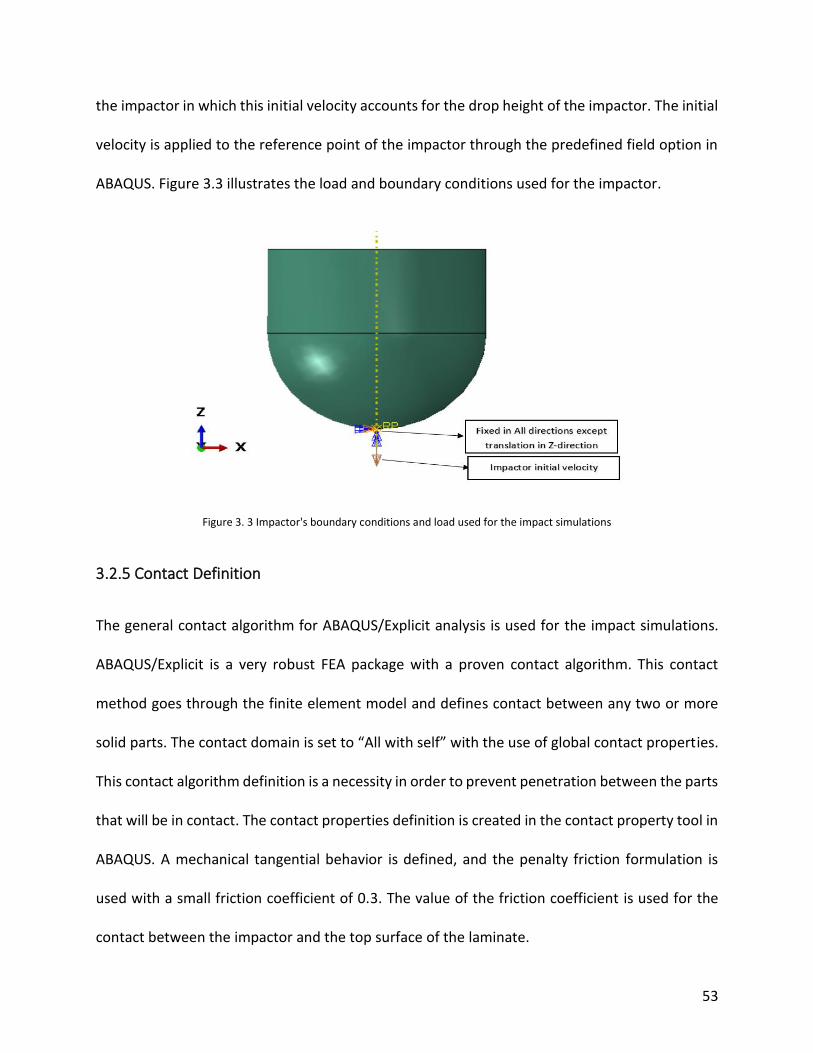
53

the impactor in which this initial velocity accounts for the drop height of the impactor. The initial

velocity is applied to the reference point of the impactor through the predefined field option in

ABAQUS. Figure 3.3 illustrates the load and boundary conditions used for the impactor.

Figure 3. 3 Impactor's boundary conditions and load used for the impact simulations

3.2.5 Contact Definition

The general contact algorithm for ABAQUS/Explicit analysis is used for the impact simulations.

ABAQUS/Explicit is a very robust FEA package with a proven contact algorithm. This contact

method goes through the finite element model and defines contact between any two or more

solid parts. The contact domain is set to “All with self” with the use of global contact properties.

This contact algorithm definition is a necessity in order to prevent penetration between the parts

that will be in contact. The contact properties definition is created in the contact property tool in

ABAQUS. A mechanical tangential behavior is defined, and the penalty friction formulation is

used with a small friction coefficient of 0.3. The value of the friction coefficient is used for the

contact between the impactor and the top surface of the laminate.

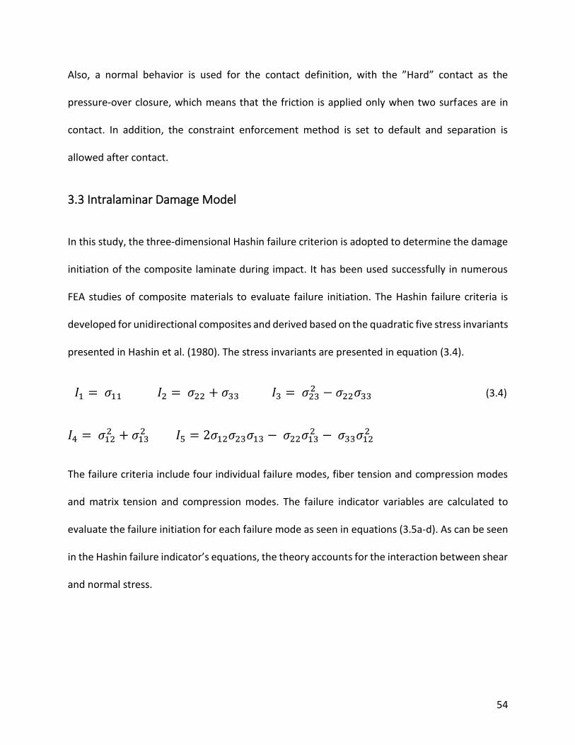
54

Also, a normal behavior is used for the contact definition, with the ”Hard” contact as the

pressure-over closure, which means that the friction is applied only when two surfaces are in

contact. In addition, the constraint enforcement method is set to default and separation is

allowed after contact.

3.3 Intralaminar Damage Model

In this study, the three-dimensional Hashin failure criterion is adopted to determine the damage

initiation of the composite laminate during impact. It has been used successfully in numerous

FEA studies of composite materials to evaluate failure initiation. The Hashin failure criteria is

developed for unidirectional composites and derived based on the quadratic five stress invariants

presented in Hashin et al. (1980). The stress invariants are presented in equation (3.4).

𝐼1 = 𝜎11 𝐼2 = 𝜎22 + 𝜎33 𝐼3 = 𝜎232 − 𝜎22𝜎33 (3.4)

𝐼4 = 𝜎122 + 𝜎13

2 𝐼5 = 2𝜎12𝜎23𝜎13 − 𝜎22𝜎132 − 𝜎33𝜎12

2

The failure criteria include four individual failure modes, fiber tension and compression modes

and matrix tension and compression modes. The failure indicator variables are calculated to

evaluate the failure initiation for each failure mode as seen in equations (3.5a-d). As can be seen

in the Hashin failure indicator’s equations, the theory accounts for the interaction between shear

and normal stress.

55

Fiber tension failure mode (FTF) (𝜎11 > 0)

𝑓1 = (𝜎11

𝑋𝑇)

2

+ 𝜎12

2 +𝜎132

𝑆𝐿2 (3.5a)

Fiber compression failure mode (FCF) (𝜎11 < 0)

𝑓2 = (𝜎11

𝑋𝐶)

2

(3.5b)

Matrix tension failure mode (MTF) (𝜎22 + 𝜎33 > 0)

𝑓3 =1

𝑌𝑇2 (𝜎22 + 𝜎33)2 +

1

𝑆𝑇2 (𝜎23

2 − 𝜎22𝜎33) + 𝜎12

2 +𝜎132

𝑆𝐿2 (3.5c)

Matrix compression failure mode (MCF) (𝜎22 + 𝜎33 < 0)

𝑓4 =1

𝑌𝐶[(

𝑌𝐶

2𝑆𝑇)

2

− 1] (𝜎22 + 𝜎33) +1

4𝑆𝑇2 (𝜎22 + 𝜎33)2 +

1

𝑆𝑇2 (𝜎23

2 − 𝜎22𝜎33) + 𝜎12

2 +𝜎132

𝑆𝐿2 (3.5d)

Where, fi is the Hashin failure indicator for each failure mode. σij are the stress components in the

material coordinate system, XT and XC are the axial tensile and compressive strength, respectively.

YT and YC are the transverse tensile and compressive strength, respectively and SL and ST are the

axial shear strength and transverse shear strength, respectively. The strength values required for

the failure initiation calculation used in equations (3.5a-d) are obtained from experimental

investigation and presented in Table 3.1.

56

3.3.1 Damage Evolution

A damage evolution law is used in this study to evaluate the intralaminar failure propagation for

each failure mode, i.e. fiber tension or compression failure mode and matrix tension or

compression failure mode. The exponential damage evolution law is adopted from Warren et al.

(2016) to calculate the damage variable for each failure mode. The damage evolution law utilizes

equation (3.6) to calculate the damage variable.

𝑑(𝑓𝑖) = 𝐷𝑖 𝑚𝑎𝑥 [1 − 𝑒𝑥𝑝 (−𝑓𝑖

𝑚

𝑚 𝑒)] (3.6)

Where Dmax is the maximum degradation variable, fi is the Hashin failure indicator, m is the

material response parameter and e is the base of the natural logarithm. Equation (3.6) can be

used to enforce different damage evolution law including instant failure or more of ductile

failure. Using a small value of the material response m would generate a ductile response of the

material damage. The damage becomes an instantaneous failure when m approaches an infinite

value. Equation (3.7) describes the instantaneous failure using the exponential damage evolution

law. The damage variable is computed for any value given by the Hashin failure indicator f.

𝑑(𝑓) = {0, 𝑖𝑓 𝑓 = 0𝐷𝑚𝑎𝑥 , 𝑖𝑓 𝑓 > 0

(3.7)

A plot of equation (3.6) is shown in Figure 3.4 with varying Hashin failure indicator f from 0 to 2.4

and specifying Dmax to be 0.8. The plot of equation (3.6) is evaluated at different values of material

response m. A value of 150 is used for the material response parameter m for the impact

simulations throughout this study.

57

Figure 3. 4 Damage variable value di as a function of the failure indicator fi using the exponential damage evolution law with Dmax

= 0.8 evaluated at various values of the material parameter m

The maximum damage variable must be specified for each Hashin failure mode. In this study, the

maximum damage variables for the tensile and compression damage modes in both fiber (D1max)

and transverse (D2max) directions are listed in equations (3.8) and (3.9). The elastic material

properties are degraded based on the maximum damage variable for each mode such that when

Dmax = 0.93, the elastic properties are degraded 7% of their original values. A property

degradation rule, which shows the Hashin failure modes along with the property that is being

degraded, is presented in Table 3.3.

𝐷1 𝑚𝑎𝑥 = {0.93, 𝑖𝑓 𝑡𝑒𝑛𝑠𝑖𝑜𝑛0.80, 𝑖𝑓 𝑐𝑜𝑚𝑝𝑟𝑒𝑠𝑠𝑖𝑜𝑛

(3.8)

𝐷2 𝑚𝑎𝑥 = {0.85, 𝑖𝑓 𝑡𝑒𝑛𝑠𝑖𝑜𝑛0.85, 𝑖𝑓 𝑐𝑜𝑚𝑝𝑟𝑒𝑠𝑠𝑖𝑜𝑛

(3.9)

0

0.1

0.2

0.3

0.4

0.5

0.6

0.7

0.8

0.9

1

0 0.2 0.4 0.6 0.8 1 1.2 1.4 1.6 1.8 2 2.2 2.4

Dam

age

Var

iab

le, d

i

Failure Indicator value, fi

m = 4

m = 10

m = 50

m=150

58

Table 3. 3 Properties degradation rule

Elastic

Property

Hashin Failure Modes

FTF FCF MTF MCF

E1 X X - -

E2 - - X X

E3 - - X X

v12 - - - -

v13 - - - -

v23 - - - -

G12 X - X X

G13 X - X X

G23 - - X X

3.4 Interlaminar Damage model

Delamination is a major failure mode for composites under impact loading and it has been

investigated by researchers both in experimental tests and numerical simulations. Sun et al.

(2014), Liu et al. (2018) and other researchers have used and proposed methods in the literature

to model delamination failure such as applying the three-dimensional delamination failure

criteria in the composite laminates. Applying the three-dimensional delamination failure criteria

in composites might lead to the inaccurate prediction of the interface properties because of the

complexity of delamination modeling. Therefore, for this study, implementing a cohesive

behavior between the interfaces becomes a better option to predict delamination between the

plies. ABAQUS has the capability to model cohesive behavior for solid elements without the need

to use subroutines to implement interlaminar failure.

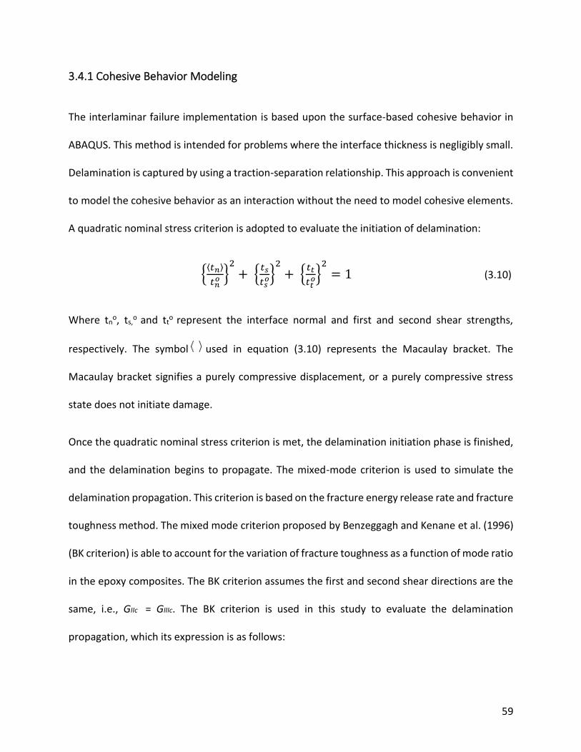
59

3.4.1 Cohesive Behavior Modeling

The interlaminar failure implementation is based upon the surface-based cohesive behavior in

ABAQUS. This method is intended for problems where the interface thickness is negligibly small.

Delamination is captured by using a traction-separation relationship. This approach is convenient

to model the cohesive behavior as an interaction without the need to model cohesive elements.

A quadratic nominal stress criterion is adopted to evaluate the initiation of delamination:

{⟨𝑡𝑛⟩

𝑡𝑛𝑜 }

2

+ {𝑡𝑠

𝑡𝑠𝑜}

2+ {

𝑡𝑡

𝑡𝑡𝑜}

2= 1 (3.10)

Where tno, ts,

o and tt

o represent the interface normal and first and second shear strengths,

respectively. The symbol used in equation (3.10) represents the Macaulay bracket. The

Macaulay bracket signifies a purely compressive displacement, or a purely compressive stress

state does not initiate damage.

Once the quadratic nominal stress criterion is met, the delamination initiation phase is finished,

and the delamination begins to propagate. The mixed-mode criterion is used to simulate the

delamination propagation. This criterion is based on the fracture energy release rate and fracture

toughness method. The mixed mode criterion proposed by Benzeggagh and Kenane et al. (1996)

(BK criterion) is able to account for the variation of fracture toughness as a function of mode ratio

in the epoxy composites. The BK criterion assumes the first and second shear directions are the

same, i.e., GIIc = GIIIc. The BK criterion is used in this study to evaluate the delamination

propagation, which its expression is as follows:

60

𝐺𝐼𝐶 + (𝐺𝐼𝐼𝐶 − 𝐺𝐼𝐶) (𝐺𝑠ℎ𝑒𝑎𝑟

𝐺𝑇)

𝜂

= 𝐺𝑇𝐶

𝐺𝑠ℎ𝑒𝑎𝑟 = 𝐺𝐼𝐼 + 𝐺𝐼𝐼𝐼 𝐺𝑇 = 𝐺𝐼 + 𝐺𝑠ℎ𝑒𝑎𝑟 (3.11)

Where GTC is the mixed-mode fracture toughness under combined mode loading and GT is the

total fracture energy release rate. GIc and GIIc denote the interfacial Mode I and II critical fracture

energy corresponding to GI and GII respectively, and ⴄ is the cohesive property parameter. The

BK criterion is activated once the total fracture energy release rate GT is equal to or greater than

the mixed-mode fracture toughness GTC. When the ratio 𝐺𝑠ℎ𝑒𝑎𝑟

𝐺𝑇 in equation (3.11) is zero, the

interlaminar failure becomes a mode I dominated. However, when the ratio 𝐺𝑠ℎ𝑒𝑎𝑟

𝐺𝑇 is one, the

interlaminar failure becomes mode II dominated. In this research, the parameter ⴄ is assumed;

however, the parameter ⴄ should be determined using a least square fit from a set of

experimental data. A plot of equation (3.11) is shown in Figure 3.5 with varying the value of the

cohesive property parameter, ⴄ.

The material properties used for the cohesive modeling are listed in Table 3.4. The strength

properties of the interface are assumed to be the epoxy matrix strength properties of PR-520.

The fracture energy of Mode I is found experimentally and presented in McDermott (2019).

However, the fracture energies of Mode II and III are assumed to be 2.4*GIc.

61

Figure 3. 5 Plot of the BK criterion with varying the value of the cohesive property parameter

Table 3. 4 Cohesive parameter used in this study

Property Value

tno (MPa) 82.1

tso (MPa) 61.4

tto (MPa) 61.4

GIC (mJ/mm2) 1.097

GIIC = GIIIc (mJ/mm2) 2.633

ⴄ 2.0

3.5 ABAQUS User Subroutine

A Fortran user subroutine (VUSDFLD) is developed to evaluate the intralaminar damage of the

composite using the proposed Hashin failure criteria with the exponential damage evolution law.

The user subroutine receives stresses from ABAQUS at every integration point and uses them to

calculate the Hashin failure indicators for each failure mode. Next, the damage variable d for each

62

mode is computed based on the exponential damage evolution law. The damage variables di are

returned to ABAQUS using the field variables tool. A look up table is defined in ABAQUS input file

to relate the field variables to the elastic material properties. Based on the returned field variable,

the appropriate material properties are assigned to the FE model. A flowchart of the

implementation of the progressive damage model corresponding to the VUSDFLD user

subroutine in ABAQUS is shown in Figure 3.6. A copy of the VUSDFLD Fortran subroutine is

attached in Appendix B.

63

Figure 3. 6 Flowchart of the implementation of the progressive damage model corresponding to the user subroutine

64

3.6 Validation of Material Model

In this section, the model validation of a single element and coupon tests is presented. This

validation is performed to ensure that the proposed progressive damage model produces

physically realistic behavior while reducing the level of complexity. The simulation models

consisted of loading for each failure mode individually and tested to verify the model response

and the damage progression. The simulations are performed with the parameter response m of

the intralaminar damage is set to be 100. The material properties used for the validation of the

material model are the homogenized properties and they are listed in Table 2.5, and the material

strengths are listed in Table 3.1.

For the single element simulations, an eight-node linear brick with dimensions of 2 mm x 2 mm

x 2 mm is modeled in ABAQUS and loaded under displacement control in each direction with

boundary conditions as shown in Figure 3.7. The stress responses of the solid element are

evaluated in the fiber, transverse and shear directions.

Figure 3. 7 Boundary conditions and loads of single element simulations: a) Fiber direction. b) Transverse direction. c) Shear direction.

65

For the simulation of the coupon tests, the FEA model is a rectangular plate generated in ABAQUS

with dimensions of 70 mm x 15 mm x 2 mm. The plate models are generated with hexahedral

solid elements and loaded in all directions, fiber, transverse and shear direction. The plate is

meshed as C3D8 with 280 elements. The boundary conditions and loads applied for each test are

shown in Figure 3.8.

Figure 3. 8 Boundary conditions and loads of coupon simulations: a) Fiber direction. b) Transverse direction. c) Shear direction.

3.6.1 Results of Model Validation

The simulation results of the single element tests loaded in tension, compression and shear

directions are illustrated in Figures 3.9. In the case of the tension in fiber direction, tension in

transverse direction and shear direction, the stresses were gradually increased until the material

reached its failure strength. Also, for the compression fiber and transverse directions, the

magnitude of the compressive stresses is gradually increased until the material reaches its failure

strength. Once the material failure occurs, the elastic properties get degraded based on the

degradation rule presented in Table 3.3.

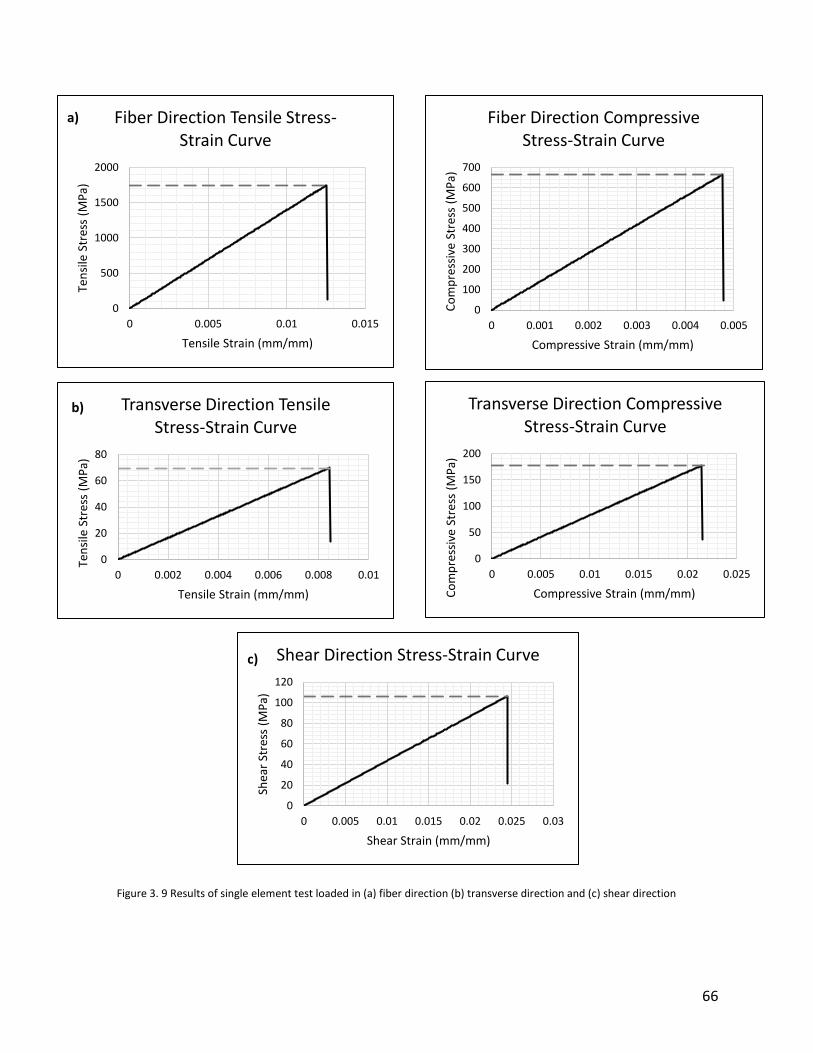
66

0

100

200

300

400

500

600

700

0 0.001 0.002 0.003 0.004 0.005

Co

mp

ress

ive

Stre

ss (

MP

a)

Compressive Strain (mm/mm)

Fiber Direction Compressive Stress-Strain Curve

0

500

1000

1500

2000

0 0.005 0.01 0.015

Ten

sile

Str

ess

(MP

a)

Tensile Strain (mm/mm)

Fiber Direction Tensile Stress-Strain Curve

a)

0

20

40

60

80

0 0.002 0.004 0.006 0.008 0.01

Ten

sile

Str

ess

(MP

a)


Transverse Direction Tensile Stress-Strain Curve

b)

0

50

100

150

200

0 0.005 0.01 0.015 0.02 0.025

Co

mp

ress

ive

Stre

ss (

MP

a)


Transverse Direction Compressive Stress-Strain Curve

0

20

40

60

80

100

120

0 0.005 0.01 0.015 0.02 0.025 0.03

Shea

r St

ress

(M

Pa)

Shear Strain (mm/mm)

Shear Direction Stress-Strain Curvec)

Figure Simulation results of single element tests: a) fiber direction b) transverse direction c) shear

direction.

Figure 3. 9 Results of single element test loaded in (a) fiber direction (b) transverse direction and (c) shear direction

67

The results of the coupon simulations are illustrated in Figures 3.10 for tension and compression

in the fiber direction, tension and compression in the transverse direction and the shear

direction. The coupon plate is loaded in tension, compression and shear directions like the single

element simulations. The coupon simulations are performed to ensure that the developed

ABAQUS user subroutine evaluates the intralaminar damage for larger models with several

numbers of elements as well as to ensure the mechanical response of the coupons is accurate.

The results of the coupon simulations are as expected. The coupons fail once the material reaches

its failure strength. It could be concluded that the response of the progressive failure model is

consistent with the expected mechanical behavior of the composite. Also, it could be concluded

that ABAQUS user subroutine can be used for practical FEA simulations.

68

0

400

800

1200

1600

2000

0 0.005 0.01 0.015

Ten

sile

Str

ess

(MP

a)


Fiber Direction Tensile Stress-Strain Curve of Rectangular Plate

a)

0

100

200

300

400

500

600

700

0 0.001 0.002 0.003 0.004 0.005 0.006Co

mp

ress

ive

Stre

ss (

MP

a)


Fiber Direction Compressive Stress-Strain Curve of Rectangular Plate

0

10

20

30

40

50

60

70

80

0 0.002 0.004 0.006 0.008 0.01

Ten

sile

Str

ess

(MP

a)


Transverse Direction Tensile Stress-Strain Curve of Rectangular Plate

b)

0

50

100

150

200

0 0.005 0.01 0.015 0.02 0.025

Co

mp

ress

ive

Stre

ss (

MP

a)


Transverse Direction Compressive Stress-Strain Curve of Rectangular

Plate

0

20

40

60

80

100

120

0 0.005 0.01 0.015 0.02 0.025

Shea

r St

ress

(M

Pa)

Shear Strain (mm/mm)

Shear Direction Stress-Strain Curve of Rectangular Plate

c)

Figure Simulation results of coupon tests: a) fiber direction b) transverse direction c) shear direction. Figure 3. 10 Results of coupon plate test loaded in (a) fiber direction (b) transverse direction and (c) shear direction

69

3.7 Impact Simulations with Damage

The FEA simulations are performed to investigate the NCF laminated composites under low

velocity impact loading. The NCF laminates are impacted at three different energy levels, 30 J, 50

J and 60 J. The parameters used for the impact simulations are listed in Table 3.5. The finite

element homogeneous ply model is subjected to the three different energy levels. While the

finite element mesoscale model is investigated under one energy level, 30 J. The numerical

impact response of the homogeneous ply model and the mesoscale model are presented and

validated with experimental data.

Table 3. 5 Impact parameters used in simulations

Impact energy (J) Drop mass (kg) Impact velocity (m/s)

30 5.498 3.303

50 9.498 3.245

60 10.498 3.381

3.8 Impact Results and Discussion

The low velocity impact simulations are performed using homogeneous ply model and mesoscale

model. This section presents a characterization of the impact simulations in terms of the force

histories, absorbed energy and damage area for low and high energy impacts.

70

3.8.1 Contact Force and Displacement Histories and Absorbed Energy

3.8.1.1 Low Energy Impact

For 30 J impact, the numerical force-time and force-displacement curves for the homogeneous

laminate are shown in Figure 3.11(a-b). The homogeneous laminate exhibits a similar impact

response with experiment, characterized by an increase in the contact force during the loading

phase with no evidence of significant damage such as drop in the contact force or high frequency

oscillations (Belingardi et al., 2002). Figure 3.11(a) shows the force-time curve, the predicted

peak force of the homogeneous ply model correlates very well with experiment with a difference

of 2.76 %. The irregular oscillating pattern is captured very well compared to experiment which

indicates that no significant damage had occurred at 30 J impact. The oscillations in the force-

time curve for the homogeneous ply model are mostly due to the plate vibration. The force-

displacement curves of the homogeneous ply model and experiment are shown in Figure 3.11(b).

The maximum deflection is under predicted by 3.09 % compared to experiment as shown in

Figure 3.11(c). The transverse displacement (deflection) of the top and bottom surfaces of the

homogeneous ply model is plotted against the in-plane X-coordinate as shown in Figure 3.12(a).

Additionally, a contour plot of the top surface and through the thickness (X-Z plane) of the

homogeneous ply model is shown in Figures 3.12(b) and (c), respectively, which illustrate the

deflection of the laminate at the peak load. It can be observed from Figure 3.11 that the rebound

response of the homogeneous ply model is slower than experiment. The total impact duration of

the homogeneous ply model is about 4.93 ms while the experiment is about 4.5 ms. The slower

rebound might be due to the accuracy of capturing the material behavior such as the model

71

indentation damage mechanism. Also, it may be caused by the friction between the impactor and

the top surface as well as the friction between the delaminated plies.

Figure 3. 11 Numerical results for the homogeneous laminate impacted at 30 J impact: (a) force-time (b) force-displacement

and (c) deflection-time curves

0

2000

4000

6000

8000

10000

12000

0 0.5 1 1.5 2 2.5 3 3.5 4 4.5 5 5.5

Forc

e (N

)

Time (ms)

Experiment

Homogeneous Model

(a)

0

2000

4000

6000

8000

10000

12000

0 0.5 1 1.5 2 2.5 3 3.5 4 4.5 5 5.5

Forc

e (N

)

Displacement (mm)

Experiment

Homogeneous Model

(b)

-5.5

-5

-4.5

-4

-3.5

-3

-2.5

-2

-1.5

-1

-0.5

0

0 0.5 1 1.5 2 2.5 3 3.5 4 4.5 5 5.5

Dis

pla

cem

ent

(mm

)

Time (ms)

Experiment

Homogeneous Model

(c)

72

(a)

(b)

(c)

Figure 3. 12 Out of plane displacement of the homogeneous ply model: (a) plot of the transverse displacement of the top and bottom surfaces against the X-coordinate, (b) X-Y plane contour plot of the top surface and (c) X-Z plane contour plot.

-6

-5

-4

-3

-2

-1

0

1

45 60 75 90 105

Tran

sver

se D

isp

lace

men

t, Z

(m

m)

X (mm)

Top Surface Bottom Surface

73

The numerical force-time and force-displacement curves of the mesoscale model are illustrated

in Figures 3.13(a) and 3.13(b), respectively and compared with the impact response of the

homogeneous ply model and experiment. The mesoscale model has predicted a larger peak force

than experiment by 21.51 %. The maximum deflection of the mesoscale model is lower than

experiment by 14.38 % as shown in Figure 3.13(c). The numerical impact results of the mesoscale

model differ from the results obtained from experiment. The difference is because the mesoscale

model requires mesh refinement in order to improve the accuracy of the results. Based on the

structural analysis presented in Section 2.3, the mesoscale model requires a large number of

elements to capture the geometry of the tows accurately and predict the structural behavior

more accurately. The current model is generated with 1,920,000 C3D8 elements and increasing

the number of elements of the mesoscale model would be computationally expensive.

74

Figure 3. 13 Numerical results for the mesoscale laminate impacted at 30 J impact: (a) force-time, (b) force-displacement and

(c) deflection-time curves

0

2000

4000

6000

8000

10000

12000

14000

16000

0 0.5 1 1.5 2 2.5 3 3.5 4 4.5 5

Forc

e (N

)

Time (ms)

Experiment

Mesoscale Model

(a)

0

2000

4000

6000

8000

10000

12000

14000

16000

0 0.5 1 1.5 2 2.5 3 3.5 4 4.5 5 5.5

Forc

e (N

)

Displacement (mm)

Experiment

Mesoscale Model

(b)

-5.5

-5

-4.5

-4

-3.5

-3

-2.5

-2

-1.5

-1

-0.5

0

0 0.5 1 1.5 2 2.5 3 3.5 4 4.5 5

Dis

pla

cem

ent

(mm

)

Time (ms)

Experiment

Mesoscale Model

(c)

75

It is observed from the force-displacement curve of the homogeneous ply model for the low

energy impact, 30 J shown in Figure 3.12(b), the homogeneous ply model does not have the

capability to accurately predict the residual displacement. This is because the permanent

deformation and the tow entanglement are not captured after impact as observed in the

experiment. In addition, it is observed that the predicted force-displacement curve is almost

enclosed by the experimental curve; this observation concludes that the predicted absorbed

energies are lower than the experimental absorbed energy. However, the force-displacement

curve of the mesoscale model is under predicted as shown in Figure 3.13(b). As previously stated,

the mesoscale model is generated with low mesh density which results in under predicting the

impact response. The plots of the absorbed energies are shown in Figure 3.14. As can be seen

from the absorbed energies plots, the homogeneous ply model curve compares very well with

experiment during the initial impact until the impactor reaches nearly zero velocity. The residual

absorbed energies get released from the impact damage during the rebound of the impactor.

Also, the under prediction of the absorbed energies is due to not capturing the residual strain

effect in the model (Lin et al., 2019). Table 3.6 summarizes the peak force, maximum deflection

and absorbed energy of the low energy impact simulations compared to experiment.

Table 3. 6 Summary of the peak force, maximum deflection and absorbed energy for the low impact energy

Impact Energy (J)/Model Peak Force (N) Maximum Deflection (mm) Absorbed Energy (J)

30

Experiment 11300.74 4.92 17.6

Homogeneous ply model

11617.20 (2.76%)

4.77 (3.09%) 10.69 (48.85%)

Mesoscale Model 14024.80 (21.51%)

4.26 (14.38%) 4.72 (115.41%)

76

Figure 3. 14 Absorbed energy vs. time curves for low impact energy, 30 J

3.8.1.2 High Energy Impact

For 50 J and 60 J impacts, the numerical and experimental force-time and force-displacement

curves are illustrated in Figure 3.15(a-b) and Figure 3.16(a-b), respectively. For the 50 J and 60 J

impacts, the peak force of the homogeneous laminate is higher than experiment by 6.57 % and

19.59 %, respectively. The maximum deflection is however under predicted for both levels of

impact energy as shown in Figures 3.15(c) and 3.16(c). Significant failure is observed

experimentally when the contact force has reached about 14,000 N for 50 J and higher. From

Figures 3.15(a) and 3.16(a), it is observed from the experimental curves that a force drop occurs

especially in the 60 J impact when the contact force has reached about 14,000 N. Once the force

drop occurs, the contact force has remained relatively constant in the range of 8000 – 12000 N

until the impactor has reached zero velocity. However, the predicted contact force of the

homogeneous ply model increases until the velocity of the impactor has reached zero. The reason

for the drop in the contact force is because a significant diagonal tows failure has been observed

0

5

10

15

20

25

30

35

0 0.5 1 1.5 2 2.5 3 3.5 4 4.5 5 5.5

Enge

rgy

(J)

Time (ms)

Experiment

Homogeneous Model

Mesoscale Model

77

experimentally in the back face (breaching of the back face) of the laminate. However, the impact

simulation using the homogeneous ply model has not captured the tows failure mechanism in

the back face of the model. This might be due to the modeling approach used to generate the

homogeneous ply model. The homogeneous plies are modeled as smeared plies (no tow and

matrix geometries involved). In addition, the interlaminar fracture energies of modes I, II and III

are another factor that influence the accuracy of the predicted results. As mentioned previously

in Section 3.2.2, the value of the interlaminar fracture energy for mode I GIC is obtained from

experiment. However, the values of the interlaminar fracture energy for modes II GIIC and III GIIIC

are assumed to be 2.4*GIC. From the literature, it is found that an accurate prediction of an

impact response is improved when an accurate value of the fracture properties is used (Tan and

Falzon et al., 2016). The exact value of mode II fracture energy is required to accurately predict

the impact response as well as the delamination/damage area (Francesconi and Aymerich et al.,

2017).

78

Figure 3. 15 Numerical results for homogeneous ply models impacted at 50 J impact: (a) force-time, (b) force-displacement and


0

2000

4000

6000

8000

10000

12000

14000

16000

0 0.5 1 1.5 2 2.5 3 3.5 4 4.5 5 5.5 6 6.5 7

Forc

e (N

)

Time (ms)

Experiment

Homogeneous Model

(a)

0

2000

4000

6000

8000

10000

12000

14000

16000

0 0.5 1 1.5 2 2.5 3 3.5 4 4.5 5 5.5 6 6.5 7

Forc

e (N

)

Displacement (mm)

Experiment

Homogeneous Model

(b)

-7

-6

-5

-4

-3

-2

-1

0

0 1 2 3 4 5 6 7

Dis

pla

cem

ent

(mm

)

Time (ms)

Experiment

Homogeneous Model

(c)

79

Figure 3. 16 Numerical results for homogeneous ply model impacted at 60 J impact: (a) force-time, (b) force-displacement and


0

2000

4000

6000

8000

10000

12000

14000

16000

18000

0 0.5 1 1.5 2 2.5 3 3.5 4 4.5 5 5.5 6 6.5 7 7.5 8

Forc

e (N

)

Time (ms)

Experiment

Homogeneous Model

(a)

0

2000

4000

6000

8000

10000

12000

14000

16000

18000

0 0.5 1 1.5 2 2.5 3 3.5 4 4.5 5 5.5 6 6.5 7 7.5 8

Forc

e (N

)

Displacement (mm)

Experiment

Homogeneous Model

(b)

-8

-7

-6

-5

-4

-3

-2

-1

0

0 1 2 3 4 5 6 7 8

Dis

pla

cem

ent

(mm

)

Time (ms)

Experiment

Homogeneous Model

(c)

80

It is observed from the force-displacement curves of the simulations for the high impact energy,

50 J and 60 J shown in Figures 3.15(b) and 3.16(b), the homogeneous ply model does not have

the capability to accurately predict the residual displacement. This is because the permanent

deformation and the tow entanglement are not captured after impact as observed in the

experiment. In addition, it is observed that the predicted force-displacement curves are almost

enclosed by the experimental curves; this observation concludes that the predicted absorbed

energies are lower than the experimental absorbed energies. The plots of the absorbed energies

are shown in Figure 3.17(a-b). As can be seen from the absorbed energies plots, the curves

compare very well with experiment during the initial impact until the impactor reaches nearly

zero velocity. The residual absorbed energies get released from the impact damage during the

rebound of the impactor. Also, the under prediction of the absorbed energies is due to not

capturing the residual strain effect in the model (Lin et al., 2019). As the impact energy increases,

a significant discrepancy is found in terms of the peak force and the absorbed energy. Table 3.7

summarizes the peak force, maximum deflection and absorbed energy for high impact energy

simulations compared to experiment.

Table 3. 7 Summary of the peak force, maximum deflection and absorbed energy for high impact energy

Impact Energy (J)/Model Peak Force (N) Maximum Deflection

(mm) Absorbed Energy

(J)

50 Experiment 13959.73 6.49 33.86


14907.70 (6.57%) 6.37 (1.87%) 20.41 (49.57%)

60 Experiment 14119.70 7.04 48.33


17186.30 (19.59%)

6.92 (1.72%) 21.95 (75.07%)

81

Figure 3. 17 Absorbed energies vs. time curves for high impact energy (a) 50 J impact and (b) 60 J impact

3.8.2 Impact Damage Area Prediction

As previously mentioned, there is a good agreement between the predicted results of the

homogeneous ply model and experiment for the 30 J impact. While for higher levels of impact

energies, 50 J and 60 J, there are some discrepancies in the numerical results of the homogeneous

ply model compared to experimental results. The predicted damage envelopes compared to the

0

10

20

30

40

50

60

0 0.5 1 1.5 2 2.5 3 3.5 4 4.5 5 5.5 6 6.5 7

Ener

gy (

mJ)

Time (ms)

Experiment

Homogeneous Model

0

10

20

30

40

50

60

70

0 0.5 1 1.5 2 2.5 3 3.5 4 4.5 5 5.5 6 6.5 7 7.5

Ener

gy (

J)

Time (ms)

Experiment

Homogeneous Model

(b)

(a)

82

experimental ultrasonic C-scan are shown in Figure 3.18(a-c). For 30 J, 50 J and 60 J impact, the

predicted damage area is mostly an elliptical shape and as the incident impact energy increases,

the damage area increases. However, the delamination area for the 50 J and 60 J impact is under

predicted. From the experimental C-scan, the delamination growth is larger than the predicted

damage. The failure mode is de-bonding in the tows of the back-face of the laminate which the

homogeneous ply model has not captured. Figure 3.19 illustrates a comparison of the damage

area between numerical and experiment. The predicted damage area measurements have been

performed using ImageJ software. As shown in the plot, the experimental damage area increases

linearly which indicates damage growth as the impact energy increases. As seen in Figure 3.19,

there is a good agreement between predicted damage area for 30 J impact and experiment.

While for 50 J and 60 J impact, a significant difference is observed in the predicted damage area

compared to experiment. This difference is due to the release of the absorbed energy during the

rebound stage of the impactor. Also, the discrepancy is because of the capability of the

intralaminar failure criteria to predict an accurate damage at higher level of energy as well as the

accuracy of the used values for the fracture energies.

83

Figure 3. 18 Predicted damage envelope compared with experimental C-scan for laminates impacted at (a) 30 J, (b) 50 J and (c) 60 J

84

Figure 3. 19 Plot of the damage area vs. incident impact energy

During impact, damage occurs in the form of fiber failure, matrix failure and delamination

between the plies. The predicted complete damage status (all failure modes) for 30 J impact in

each lamina of the homogeneous ply model, starting from the top ply (impact region) to bottom

ply is shown in Figure 3.20. The “rotating fan” damage pattern is predicted on the top few plies

where the damage occurs perpendicular to the fiber direction as seen in Figure 3.20. The different

damage modes for 30 J impact of the homogeneous ply model are shown in Figure 3.21. It is

observed that most of the damage at the top plies are compression fiber failure as well as

compression matrix failure. Whereas the tension failure modes, fiber and matrix, start to occur

from the back surface of the laminate and progress toward the top surface. The topmost plies

(impact region – under the impactor) have little fiber damage compared to matrix damage. A

similar damage pattern of the rotating fan is predicted for the 50 J and 60 J impacts. Figures 3.22

and 3.23 illustrate the first eight plies as well as the through thickness damage for different

0

500

1000

1500

2000

2500

3000

20 30 40 50 60 70

Dam

age

Are

a (m

m2

)

Impact Energy (J)

Homogeneous Model

Experiment

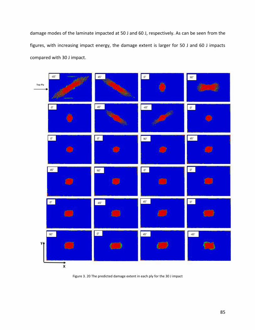
85

damage modes of the laminate impacted at 50 J and 60 J, respectively. As can be seen from the

figures, with increasing impact energy, the damage extent is larger for 50 J and 60 J impacts

compared with 30 J impact.

Figure 3. 20 The predicted damage extent in each ply for the 30 J impact

86

Figure 3. 21 Predicted through thickness damage contour for different damage modes for 30 J impact

Figure 3. 22 Predicted damage contour of the laminate impacted at 50 J

87

Figure 3. 23 Predicted damage contour of the laminate impacted at 60 J

The progressive damage of the homogeneous ply model during the 30 J impact event is shown in

Figure 3.24. The time intervals are marked on the force-time curve and illustrated in Figure 3.24

(a). The progressive damage growth for different failure modes, fiber and matrix failure modes,

of the homogeneous ply model is shown in Figures 3.24 (b) and (c). The damage of the

homogeneous ply model grows steadily until the peak load, point (e). At the peak load (e) and

beyond the peak load state, the extent of the damage is reached its final state, completely

damaged.

88

(a)

(b)

(c)

Figure 3. 24 The progressive damage growth of a homogeneous ply model impacted at 30J: (a) force-time curve, (b) fiber damage growth and (c) matrix damage growth

0

2000

4000

6000

8000

10000

12000

14000

0 0.5 1 1.5 2 2.5 3 3.5 4 4.5 5 5.5

Forc

e (N

)

Time (ms)

a

c

d

e

f

g

b

89

3.8.3 Conclusion

The NCF homogeneous ply laminate and mesoscale laminate are used to predict the low velocity

impact response. The laminated composites are impacted at three different energy levels 30 J,

50 J and 60 J. The numerical results are validated with experimental results in terms of the force

histories, absorbed energy and damage/delamination area. Excellent agreement is observed in

terms of peak force, maximum deflection and damage area between homogeneous ply laminate

and experiment for the 30 J impact with an overall error percentage less than 3 %. However, the

mesoscale laminate is impacted at 30 J and the impact response is under predicted compared to

experiment. The mesoscale laminate model requires mesh refinement to improve the accuracy

of the impact response results. In the case of higher impact energies, 50 J and 60 J, the

homogeneous ply model under predicts the impact response. It is observed that the level of

accuracy decreases as the level of impact energy increases. The under prediction of the impact

response is due to the accuracy of capturing the material behavior (damage) under impact

loading. The fracture energies of mode II and III have to be determined experimentally in order

to predict an accurate material behavior under the low velocity impact loading. In addition, the

absorbed energies are under predicted in the case of low as well as high impact energy, and this

is due to the released damage energy during the rebound phase of the impactor, and the residual

strain effect is not captured in the models. Overall, based on the presented results of the low

velocity impact, it can be concluded that the homogeneous ply model is reliable to predict the

impact response up to 50 J impact energy.

90

Chapter 4 Predicting the Compression After Impact Performance

of Multidirectional Fiber-Reinforced Laminate

4.1 Introduction

The accurate prediction of damage tolerance in fiber reinforced composite plays a significant role

in reducing the weight of aerospace structures, especially in civil aircraft (Megat-Yusoff et al.,

2019). The damage tolerance is studied to determine the effect of impact energies on the residual

strength of the composites. The compression after impact (CAI) behavior of laminated structures

is used/evaluated to measure the residual strength of composite structures (Tuo and Zhang et

al., 2019). In this chapter, the proposed FE models for predicting the CAI response of the NCF

composites are presented. The modeling of the FE NCF laminates is presented in Chapter 2. The

CAI simulations are performed to measure the damage tolerance of the FE laminates after being

damaged by low velocity impact. The composite laminates are subjected to an axial compression

load to predict the compressive residual strength of the composites. The first step is to induce

damage to the laminates using low velocity impact as presented in Chapter 3. This is then

followed by a compression simulation of the damaged laminates. The CAI simulations utilize the

progressive damage models detailed in Chapter 3 to predict the intralaminar and interlaminar

failure. All experimental data presented in this Chapter are obtained from McDermott (2019) and

used for the validation of the FE models for the CAI simulations.

91

4.2 Compression After Impact Methodology

The damage and failure models implemented to predict the intralaminar failure of the laminates

utilize the 3D Hashin failure criteria to predict failure initiation and the exponential damage

evolution law used to compute the damage variables for each failure mode. For the interlaminar

failure, the quadratic stress criterion and the Benzeggagh and Kenane (BK) law are used to predict

damage initiation and damage propagation, respectively. The damage models of the intralaminar

and interlaminar failure are presented in detail in Chapter 3.

The CAI simulations are performed using ABAQUS/Explicit since it was used for the low velocity

impact simulations. Instead of using ABAQUS/Implicit solver method for the CAI simulations

(Quasi-static CAI), the ABAQUS/Explicit solver is implemented to avoid the complexity of

converting the damaged model from the Explicit impact simulation to Implicit solver. In addition,

the use of ABAQUS/Explicit would eliminate the conversion issue of ABAQUS/Implicit solver since

there is non-linear behavior involved in the model.

As mentioned previously, the CAI simulation is carried out to study the effect of the impacted

laminates on their residual strength. First, the damage of the laminates is induced using a low

velocity impact as presented in Chapter 3. Once the impact simulations are completed, the

composite laminates are subjected to axial compression to assess their damage tolerance.

However, in order to predict an accurate response of the compression after impact, an

intermediate process is performed to import the results from the impacted laminate to the CAI

model as an initial state. The ABAQUS command “ *Import ” is used to import the results obtained

from the impact simulations to the CAI model. The *Import command has the capability to import

92

the stresses, strains and displacement to the CAI model. Additionally, this command is able to

import the results of the intralaminar failure such as the field/damage variables and state

variables (failure indicators) for each element as well as the delamination failure variable to the

CAI model from the impacted laminate. To ensure that the results from the impacted laminate

get imported accurately as an initial state to the CAI model, the CAI model has to be the same as

the impacted laminate in terms of the number of elements, element type and part instances’

name. Figure 4.1 illustrates a schematic of ABAQUS analysis steps.

Figure 4. 1 A schematic of ABAQUS analysis steps

The laminated composite models are simulated in two sequential steps as follow:

1) Impact step: simulation of the impact loading and evaluation of the impact damage.

2) CAI step: the results from the impacted laminate are imported as an initial state to the

CAI model and then the simulation of the CAI is performed until the model’s failure.

93

In the second step, the results of the impacted laminate are imported on the CAI model where

new boundary conditions are applied to perform the CAI simulations. The model dimensions, CAI

setup and boundary conditions used for the simulations are shown in Figure 4.2. The dimensions

of the composite plate used in the CAI simulations are 150 mm x 100 mm x 4.464 mm. The

boundary conditions are applied based on the experiment setup where the Airbus test fixture

(AITM 1-0010) is used to carry out the compression tests. The top and bottom regions are

restrained in the thickness direction with the displacement component U3=0. The bottom face is

constrained such that there is no translation in 1-direction U1=0 (vertical translation). One node

at the bottom face is constrained in the horizontal translation such that U2=0. The knife/side

edges are simply supported through the thickness such that the displacement component U3=0.

The side edges are 115 mm long and they are 5 mm apart from the outer perimeter of the model.

The prescribed load is applied as a displacement control at a constant load rate of 13.5 m/min in

ABAQUS and it is applied on a reference point. The nodes of the top face are constrained to the

motion of the reference point using the kinematic coupling constraint feature in ABAQUS.

94

Figure 4. 2 Virtual CAI test setup of the FE model

4.3 Stress and Strain Calculations

The compressive stress-strain response for the composite laminates is calculated based on the

reaction force and the displacement of the point load of the model. This approach is adopted so

that an average stress and strain is determined for the whole model. The average stress and

strain equations are shown in Equation (4.1) and (4.2), respectively.

𝜎 = 𝑅𝐹

𝐴 (4.1)

𝜀 = 𝛿

𝐿 (4.2)

1 - Top and bottom regions are restrained such that U3 = 0. The width of the area is 10 mm. 2 - Side edges (Knife edges) are simply supported U3 = 0. 3 - Bottom face: translation in 1 is fixed U1=0.

95

where RF is the reaction force of the load reference point, A is the cross-sectional area of the

region where the load is applied, δ is the change in displacement and L is the length of the model.

In the current model, the cross-sectional area A = 446.4 mm2and the length of the model L = 130

mm.

4.4 Results and Discussion

The predicted compressive stress-strain responses for undamaged homogeneous ply and

mesoscale models are shown in Figure 4.3 and summarized in Table 4.1. As seen in the figure and

Table 4.1, the predicted moduli of the homogeneous ply model and mesoscale model are higher

than the results obtained from experiment by 11.29 % and 12.57 %, respectively. The predicted

compressive ultimate strength of the undamaged homogeneous ply laminate is higher than

experiment by 2.69 %. However, for undamaged mesoscale laminate, the predicted ultimate

strength is lower than experiment by 16.75 %. The under prediction of the ultimate strength for

the mesoscale model is due to the inability of the mesoscale model to capture the tow

geometries precisely, for more detail on the discussion of the mesoscale geometries is presented

in Chapter 2 and 3.

As mentioned previously, in order to predict the compressive residual strength of the laminate

accurately, it is important to first capture the impact response accurately. Based on the impact

numerical results presented in Chapter 3, the impact response of the homogeneous ply laminate

impacted at 30 J correlates very well with experiment in terms of peak force, maximum

deflection, absorbed energy and damage area. Therefore, the homogeneous ply laminate

impacted at 30 J is taken to a further step to measure the damage tolerance of the laminate after

96

impact. The comparison of the compressive stress-strain response between numerical and

experiment for 30 J CAI test is shown in Figure 4.4. The predicted stress-strain response of

homogeneous laminate for 30 J CAI correlates very well with experiment. The predicted

compressive residual strength, listed in Table 4.1, is lower than experiment by 4.75 %. The effect

on the ultimate strength is shown in Figure 4.4 of the impacted laminate where a lower ultimate

strength is predicted compared to the undamaged result of the homogeneous ply model

illustrated in Figure 4.3. A summary of the predicted and experimental moduli is listed in Table

4.1 where the percentages are the difference between numerical and experiment. The moduli

for the laminates are predicted and compared with experiment, the predicted and experimental

moduli are computed in the range of 0.1 % to 0.3 % strain. The experimental values presented

are the average value of four to five tested specimens. The predicted moduli are higher than

experiment as seen in Table 4.1. The reason for obtaining low compressive modulus

experimentally can be due to the difference between the setup of the test and the boundary

conditions used for numerical simulations. Another reason for obtaining different moduli is

because of the material behavior of the composite under compression test. For instance, there

is a tendency for micro buckling of carbon fibers subjected to compression load which has been

noticed experimentally (Mujika et al., 2006).

97

Figure 4. 3 Compressive stress-strain responses for undamaged homogenous model and mesoscale model

Figure 4. 4 Compressive stress-strain responses for 30 J CAI test of homogeneous ply model

0

50

100

150

200

250

300

350

400

0 0.1 0.2 0.3 0.4 0.5 0.6

Stre

ss (

MP

a)

Strain (%)

Specimen1

Specimen2

Specimen3

Specimen4

Mesoscale Model

Homogeneous Model

0

50

100

150

200

250

300

0 0.1 0.2 0.3 0.4 0.5

Stre

ss (

MP

a)

Strain (%)

Specimen1

Specimen2

Specimen3

Specimen4

Specimen5

Homogeneous Model

98

Table 4. 1 Results summary of CAI

Energy Level / Model Ultimate Strength (MPa) Modulus (GPa)

0 J

Experiment 335 65

Homogeneous ply model 344.12 (2.69%) 72.78 (11.29%)

Mesoscale Model 283.21 (16.75%) 73.72 (12.57%)

30 J Experiment 250 63.50

Homogeneous ply model 238.39 (4.75%) 68.49 (5.0%)

4.5 Conclusions

The compressive residual strength of the homogeneous ply model impacted at 30 J is predicted.

Good agreement is observed between the CAI of the homogeneous ply model and experiment.

The predicted compressive residual strength of the homogeneous ply laminate impacted at 30 J

is within 4.75 % of the averaged experimental value. For the undamaged CAI simulations, the

homogeneous ply laminate demonstrates a better prediction of the ultimate strength compared

to the mesoscale laminate. The predicted moduli of the laminates are higher than experiment.

The difference between the numerical and experimental results is due to the application of the

boundary conditions. In addition, the difference between the numerical and experimental moduli

is because of the material behavior of the composite under compression test such that the

composite laminate might experience a micro buckling of the fibers during the experiment and it

was not captured numerically (Mujika et al., 2006). Overall, the homogeneous ply laminate

showed excellent performance in terms of predicting the compressive residual strength for a

laminate impacted at 30 J as well as the undamaged compressive strength.

99

Chapter 5 Conclusions and Future Work/Recommendations

5.1 Conclusions

In this thesis, numerical tools are used to investigate fiber-reinforced composites under low

velocity impact loading and predict the compressive residual strength of the laminate after

impact. Finite element NCF models are developed to study their mechanical behavior under

impact loading. The NCF models are generated using two approaches. First approach, a finite

element homogeneous ply laminate is generated where in this model there is no difference in

the model’s constituent. Second approach, a finite element mesoscale model as a plate which

consists of tows geometries as well as matrix geometries where the constituents of the plate are

considered as different parts.

Chapter 3 presents the modeling and results of the low velocity impact simulations. The finite

element homogeneous ply laminate is impacted at three different levels of impact energy 30 J,

50 J and 60 J. While the finite element mesoscale laminate is impacted at only 30 J because it is

computationally expensive due to the large number of elements used to generate the mesoscale

model. The presented numerical results are validated with experimental data in terms of the

peak force, absorbed energy, maximum deflection and damage area. It is observed that the

predicted impact response of the mesoscale model does not correlate well with the experimental

data. In order to have an accurate impact response of the mesoscale model, a mesh refinement

has to be performed to the mesoscale model where a large number of elements is required to

capture the geometries of the model, e.g. tow geometries and matrix geometries. Based on the

100

convergence study presented in Chapter 2, the mesoscale model requires over 10,000,000

elements to produce accurate results whereas the current mesoscale model is generated with

1,920,000 elements. However, the homogeneous ply model showed excellent agreement with

experimental data up to 50 J impact energy. In the case of higher impact energies, 50 J and 60 J,

the homogeneous ply model over predicted the peak forces and under predicted the progressive

damage of the laminate compared to experiment. The discrepancy between the numerical and

experiment for higher levels of impact energy might be due to the inaccuracy of some of the

assumed parameters such as the interlaminar material properties. Based on the literature

presented in Chapter 1, it is found that the values of the fracture energies used in simulations

play an important key to capture the overall impact response.

Chapter 4 presents the modeling and results of the compression after impact. The compressive

ultimate strength is predicted for undamaged mesoscale model as well as undamaged

homogeneous ply model. The predicted ultimate strength for the undamaged homogeneous ply

model is in good agreement with experiment with a difference of 2.69 %. However, the

mesoscale model under predicts the ultimate strength compared to experiment by 16.75 %. The

compressive residual strength after impact is predicted for homogeneous ply laminate subjected

to 30 J impact. The predicted compressive residual strength correlates well with experiment with

a difference of 4.75 %. In addition, the laminates moduli are calculated and listed in Table 4.1.

The predicted Young’s moduli are higher than the experimental values. The difference in the

numerical and experimental moduli may be due to the application of the boundary conditions.

Also, the difference between the numerical and experimental moduli is because of the material

behavior of the composite under compression test such that the carbon fibers of the specimen

101

might experience a micro buckling during the experiment and it was not captured numerically

(Mujika et al., 2006).

From the results presented in Chapters 3 and 4, it can be concluded that the homogeneous ply

model can be used to perform low velocity impact simulations and predict the compressive

residual strength of the laminate. It is computationally efficient to use a homogeneous ply model

since it does not require a large number of elements to predict the impact response as well as

the compressive residual strength. Based on the results presented, the homogeneous ply

laminate can predict an accurate low velocity impact response up to 50 J impact energy. There

are still more improvements that can be done to improve the accuracy of the results as well as

to reduce the cost of the simulations.

5.2 Future Work/Recommendations

The finite element simulations require additional work to accurately predict the progressive

damage of the laminates. Additional implementations are presented below that would be

beneficial for improving the accuracy of the results.

1. The modeling technique used to generate the homogeneous ply model and the mesoscale

model can be revised. A small impact region (homogeneous/mesoscale region) can be

generated with fine mesh surrounded by a homogeneous region generated with coarse

mesh. The impact region and the surrounded region is connected through a “tie

constraint” to control the motion between the two regions. This approach would make

the simulations more efficient which will lower the cost of running the simulations.

102

2. The accuracy of the finite element simulations depends on the values of fracture energy.

To improve the interlaminar damage prediction, it is very important to measure the

fracture energy experimentally and use the values in the modeling to simulate an accurate

impact response as well as predict the compressive residual strength. In addition, the

cohesive response parameter ⴄ should be obtained based on experimental data of

fracture energy to predict delamination more accurately.

3. A criterion should be implemented to account for the residual strain that would capture

the permanent deformation.

4. For predicting the compressive residual strength of the laminate after impact, it is

recommended to stabilize the laminate (i.e. use Rayleigh damping) after impact and then

import the damage from impact to the CAI model.

103

REFERENCES

ABAQUS. (2017). ABAQUS User's Manual, Dassault Systemes Simulia Corp.

Abir, M., Tay, T., Ridha, M., & Lee, H. (2017). Modelling Damage Growth in Composites

Subjected to Impact and Compression after Impact. Composite Structures, 168, 13-25.

Abrate, S. (2011). Impact Engineering of Composite Structures.

Barbero, E. J. (2011). Introduction to Composite Materials Design .

Belingardi, G., & Vadori, R. (2002). Low Velocity Impact Tests of Laminate Glass-Fiber-Epoxy

Matrix Composite Material Plates. International Journal of Impact Engineering, 27, 213-

229.

Benzeggagh, M., & Kenane, M. (1996). Measurement of Mixed-Mode Delamination Fracture

Toughness of Unidirectional Glass/Epoxy Composites with Mixedmode Bending

Apparatus. Composites Science and Technology, 56(4), 439-449.

Breen, C., Guild, F., & Pavier, M. (2006). Impact Damage to Thick Carbon Fiber Reinforced

Plastic Composite Laminates. Journal of Materials Sience, 41, 6718-6724.

Carruthers, J., Kettle, A., & Robinson, A. (1998). Energy Absorption Capability and

Crashworthiness of Composite Material Structures: Review. Applied Mechanics Review,

51, 635-649.

CYCOM PR 520 RTM RESIN SYSTEM. (n.d.). Retrieved from https://www.e-

aircraftsupply.com/MSDS/111329CYCOM%20PR520%20RTM%20tds.pdf

Dogan, F., Hadavinia, H., Donchev, T., & Bhonge, P. (2012). Delamination of Impacted

Composite Structures by Cohesive Zone Interface Elements and Tiebreak Contact.

Central European Journal of Engineering, 2(4), 612-626.

Falzon, B. G., Tan, W., Price, M., & Liu, H. (2016). The Role of Material Characterisation in the

Crush Modelling of Thermoplastic Composite Structures. Composite Structures, 153,

914-927.

Findlay, S., & Harrison, N. (2002). Why Aircraft Fail. Materials Today, 18-25.

Francesconi, L., & Aymerich, F. (2017). Numerical simulation of the Effect of Stitching on the

Delamination Resistance of Laminated Composites Subjected to Low-Velocity Impact.

Composite Structures, 159, 110-120.

González, E., Maimí, P., Camanho, P., Turon, A., & Mayugo, J. (2012). Simulation of Drop-Weight

Impact and Compression after Impact Tests on Composite Laminates. Composite

Structures, 94, 3364–3378.

104

Guo, W., Xue, P., & Yang, J. (2013). Nonlinear Progressive Damage Model for Composite

Laminates Used for Low-Velocity Impact. Applied Mathematics and Mechanics, 34,

1145-1154.

Hashin, Z. (1980). Failure Criteria for Unidirectional Fiber Composites. Journal of Applied

Mechanics, 47, 329-334.

HEXCEL. (n.d.). HexTow IM7 Carbon Fiber . Retrieved from

https://www.hexcel.com/user_area/content_media/raw/IM7_HexTow_DataSheet.pdf

Hirai, Y., Hamada, H., & Kim, J. (1998). Impact Response of Woven Glass Fabric Composites-I.

Effect of Fiber Surface Treatment . Composites Science and Technology, 91-104.

Hou , J., Petrinic, N., Ruiz, C., & Hallett, S. (2000). Prediction of Impact Damage in Composite

Plates. Composites Science and Technology, 60, 273-281.

Hull, D. (1991). Unified Approach to Progressive Crushing of Fiber-Reinforced Composite Tubes.

Composite Science and Technology, 40, 377-421.

Li, S. (2001). General Unit Cells for Micromechanical Analyses of Unidirectional Composites .

Composites Part A, 32(6), 815-826.

Lin, S., & Waas, A. M. (2019). Experimental and Numerical Study on the Low Velocity Impact

Damage of a Shear Dominated Composite Laminate. AIAA Scitech 2019 Forum.

Liu, H., Falzon, B. G., & Tan, W. (2018). Predicting the Compression-After-Impact (CAI) Strength

of Damage-Tolerant Hybrid Unidirectional/Woven Carbon-Fibre Reinforced Composite

Laminates. Composites Part A, 189-202.

Long, A C and Brown, L P. (2011). Composite reinforcements for optimum performance: Modelling the geometry of textile reinforcements for composites: TexGen, edited by P. Boisse, Woodhead Publishing Ltd, ISBN: 978-1-84569-965-9.

Maio, L., Monaco, E., Ricci, F., & Lecce, L. (2013). Simulation of Low Velocity Impact on

Composite Laminates with Progressive Failure Analysis. Composite Structures, 103, 75-

85.

Mathivanan, N. R., & Jerald, J. (2010). Experimental Investigation of Low-Velocity Impact

Characteristics of Woven Glass Fiber Epoxy Matrix Composite Laminates of EP3 Grade.

Materials and Design, 31, 4553-4560.

Matzenmiller, A., Lubliner, J., & Taylor, R. (1995). A Constitutive Model for Anisotropic Damage

in Fiber-Composites. Mechanics of Materials, 125-152.

McDermott, J. Damage Resistance and Tolerance of 3D Woven Composites. Master thesis, 2019.

105

Megat-Yusoff, P., Shah, S., Karuppanan,, S., & Sajid, Z. (2019). Impact Resistance and Damage

Tolerance of Fiber Reinforced Composites: A Review. Composite Structures, 217, 100-

121.

Mujika, F., Carbajal, N., Arrese, A., & Mondragon, I. (2006). Determination of Tensile and

Compressive Moduli by Flexural Tests. Polymer Testing, 25, 766-771.

Naik, N. K., & Shrirao, P. (2004). Composite Structures under Ballistic Impact. Composite

Structures, 66, 579-590.

Omairey, S. L., Dunning, P. D., & Sriramula, S. (2019). Development of an ABAQUS Plugin Tool

for Periodic RVE Homogenisation. Engineering with Computers, 35, 567-577.

Perillo, G., & Jørgensen, J. K. (2016). Numerical/Experimental Study Of The Impact and

Compression After Impact On GFRP Composite For Wind/Marine Applications. Procedia

Engineering, 167, 129-137.

Pernas-Sánchez, J., Pedroche , D., Varas, D., López-Puente, J., & Zaera, R. (2012). Numerical

Modeling of Ice Behavior under High Velocity Impacts. International Journal of Solids

and Structures, 49, 1919-1927.

Prichard, J., & Hogg, P. (1990). The Role of Impact Damage in Post-Impact Compression Testing.

Composites, 21, 503-511.

Safri, S., Sultan, M., Yidris, N., & Mustapha, F. (2014). Low Velocity and High Velocity Impact

Test on Composite Materials – A review. The International Journal of Engineering and

Science, 3(9), 50-60.

Sjoblom, P., HARTNESS, J., & CORDELL, T. (1998). On Low-Velocity Impact Testing of Composite

Materials. Journal of COMPOSITE MATERIALS, 22, 30-52.

Sun, X., & Tong, M. (2015). Finite Element Analysis of Low-Velocity Impact Damage on Stiffened

Composite Panels. International Journal of Aerospace and Mechanical Engineering,

1259-1263.

Topac, O., Gozluklu, B., Gurses, E., & Coker, D. (2017). Experimental and Computational Study

of the Damage Process in CFRP Composite Beams under Low-Velocity Impact.

Composites: Part A, 92, 167-182.

Tuo, H., Lu, Z., Ma, X., Xing, J., & Zhang, C. (2019). Damage and Failure Mechanism of Thin

Composite Laminates under Low-Velocity Impact and Compression-after-Impact Loading

Conditions. Composites Part B, 163, 642-654.

Vaidya, Uday K. (2011). Impact Response of Laminated and Sandwich Composites. [book auth.] Serge Abrate. Impact Engineering of Composite Structures . Brimingham : Springer Wien New York , 97-191.

106

Waas, A. M., Thorsson, S. I., & Rassaian, M. (2018). Low-Velocity Impact Predictions of

Composite Laminates using a Continuum Shell Based Modeling Approach Part b: BVID

Impact and Compression after Impact. International Journal of Solids and Structures,

201-212.

Warren, K., Lopez-Anid0, R., Vel, S., & Bayraktar, H. (2016). Progressive Failure Analysis of

Three-Dimensional Woven Carbon Composites in Single-Bolt, Double-Shear Bearing .

Composites Part B, 84, 266-276.

Zhang, C., Li, N., Wang, W., Binienda, W., & Fang, H. (2015). Progressive Damage Simulation of

Triaxially Braided Composite using a 3D Meso-scale Finite Element Model. Composite

Structures, 125, 104-116.

Zumpano, G., Stronge, W., & Sutcliffe, M. (2008). Impact Damage in Hybrid Braided Twill

Composites. Journal of Materials Science, 43, 6668-6675.

107

APPENDICES

APPENDIX A: TexGen Scripts

A.1 A Python script to generate a unit cell model in TexGen

108

A.2 A Python script to generate NCF mesoscale model in TexGen

111

APPENDIX B: ABAQUS (VUSDFLD) Subroutine

B.1 VUSDFLD subroutine used for a homogeneous ply model

115

B2. VUSDFLD subroutine used for a mesoscale model

120

BIOGRAPHY OF THE AUTHOR

Maitham Alabbad was born in Alahsa, Saudi Arabia. He received his primary education in Saudi

Arabia and graduated from Aljafr High School in 2010. He obtained his B.S. degree in Mechanical

Engineering from the University of Maine in 2017. Maitham worked as a graduate research

assistant in the field of Solid Mechanics, and as a graduate teaching assistant for the Department

of Mechanical Engineering. Maitham Alabbad is a candidate for the Master of Science degree in

Mechanical Engineering from the University of Maine in May 2020.

Impact Resistance of Fiber-Reinforced Composites Using ...

Documents

Transcript of Impact Resistance of Fiber-Reinforced Composites Using ...