IMPACT OF THE GLOBAL FINANCIAL CRISIS ON THE EXPORT …ijeronline.com/documents/volumes/Vol 5 iss...

IMPACT OF THE GLOBAL FINANCIAL CRISIS ON THE EXPORT SECTOR OF INDIA - A VECM APPROACH Ronit Mukherji, M.Sc Economics, Warwick University

[email protected], +447438595485

______________________________________________________________________________ ABSTRACT This paper tries to analyze the impact of the global financial crisis on the export sector of India using a vector error correction model. This paper tries to determine a long run relationship between India’s export sector and the Gross Domestic Product of the U.S.A. to see how a slowdown in the U.S. economy has adversely affected our exports. We find convincing evidence that a positive long run relationship does exist between this two key variables. Also impulses generating from U.S. economy have permanent effects on the Indian economy and export sector. JEL C32, F14, F44 KEYWORDS - GLOBAL FIANCIAL CRISIS, EXPORT SECTOR ______________________________________________________________________________ INTRODUCTION AND BRIEF LITERATURE REVIEW The global financial crisis (GFC) which originated in the US in 2008 affected almost all countries, some more than others. During the incubation period of the financial crisis, the financial market of US remained a one-way causation relation with most other countries. The financial crisis of US released powerful impulse waves to the outside world and many countries could not avoid the infection of the crisis.

In a globalised economy, recession in the developed countries would invariably impact the export sector of emerging economies like India. After 2008 there has been a dramatic deterioration in the export performance of India as over 27% of her exports are directed towards the US (2007-08). The current account deficit reached at 2.6% of the GDP which is the highest since 1991. The Indian government had to scale down the export target for the year 2008-09 to $175 billion from $200 billion and had to do the same for 2009-10 (Rajya Sabha Secretariat). The crisis led to a severe decrease in demand for Indian goods. Exports across all sectors from agriculture to manufacturing to services witnessed a sharp downward movement. The effect was not confined to the export sector as the economic growth of India decelerated to 6.7% which was a 2.1% decline from the 5 year average (Indian Economic Survey, 2009-10). These effects were still muted due to the overall strength of the domestic demand and the predominant domestic financing of investment.

Most of the previous literature on export sector of India focuses mainly on testing whether India is a case of export led growth, supporting the view of Bhagwati, 1978 and Kruger, 1978 (Pradhan, RBI Papers, 2010). Or if there is evidence that the growth led export hypothesis of Thornton, 1996 is applicable in the Indian scenario (Mishra, P. K. (2011). Support to the former would mean that the slowdown in exports explains the slower economic growth of India, whereas a tendency towards the latter would mean that it is the economic slowdown which is responsible for India’s poor export performance, post the global financial Crisis.

In the paper by Cynthia P. Cudia (2012) a VAR approach is used to determine the effect of GFC on the export performance of Philippines (which like India trades significantly with USA) and it concludes that shocks in the Philippine export sector are significantly and negatively generated by the shocks on its own GDP whereas not so significantly when it comes to the economic health

Ronit Mukherji, Int.J.Eco. Res., 2014, v5i3, 10-21 ISSN: 2229-6158

IJER | MAY - JUNE 2014 Available [email protected]

10

mailto:[email protected]�

of US measured in their GDP. However Philippine GDP is adversely affected by negative shocks to the US GDP.

This study undertakes a Vector error correction Model (VECM) approach to finding a relationship between the US GDP and the Export performance of India both in the short and long run to understand why the GFC has had such an adverse impact. The error correction model (ECM) was first suggested by Granger in the Journal of Econometrics (1981) and was later extended by Granger and Engel in Econometrica (1987) to develop estimation procedures, tests and empirical application after testing for the presence of cointegration. This paper also tries to determine how a shock (crisis of 2008) in the US GDP influences the exports and GDP of India through an impulse response.

DATA AND METHODOLOGY

For the study I have used annual time series data from 1970 to 2012, sourced from Reserve Bank of India (RBI) Database on the Indian Economy and World Bank website. Variables considered for study are Gross Domestic Product of India in Billion rupees (GDPI), the Total Export of all Commodities by India (TEI), Gross Domestic Product of United States of America (GDPU) in the same unit and the Exchange Rate in terms of Indian Rupee given per unit US Dollar (EXRU). Natural logarithmic transformations of the variables are considered to stabilise the variance of the series and for better estimation. A log-log functional form aids the calculations of elasticity. It also helps overcome the scale effect present in the variables selected. A graphical representation is given :-

05

1015

Log

of v

aria

bles

1970 1980 1990 2000 2010Years

Log of GDP at factor cost- IndiaLog of Total export of commodities-IndiaLog of GDP at factor cost-USALog of Rupee per unit of dollar

Trend in VariablesGraph-1



11

From the graph above we observe that there is a trend in the variables under consideration so we run an Augmented Dickey Fuller test (ADF) (Dickey, Fuller 1979) with a trend component specified in it and with 3 lags. [Final prediction error (FPE), Akaike's information criterion (AIC) and the Lagrange test determine that there ought to be 4 lags, whereas Hannan and Quinn’s information criterion (HQIC) and Schwartz’s Bayesian information criterion (SBIC) statistics determine that there ought to be 1 lag in the model. Lütkepohl (2005) has shown that HQIC and SBIC provide consistent estimates of the true lag length for large number of observations whereas the others tend to overestimate it. Thus factoring in everything I have decided to go with 3 lags]. The test will help us test the Null Hypothesis of a unit root versus the alternative that there is no unit root meaning that the time series under consideration is stationary. We test for significance at the 5% level and any time the absolute value of the test statistic is greater than the respective critical value, we can reject the null hypothesis. We test for stationarity of the first differenced series using the Philips-Perron test and again the ADF test. Details are summarized below:-

Variables Test Statistic First-Difference (PPerron) Order of

Table-1

(In Logs) (Critical Value) Zt (-2.955) Zrho (-13.012) Integration

1) GDPI -3.524 -4.719 -27.877 I (1)

(-3.545)

2) TEI -2.494 -6.061 -43.801 I (1)

(-3.544)

3) EXRU -1.975 -4.390 -27.683 I (1)

(-3.544)

4) GDPU -0.891 -4.466 -28.169 I (1)

(-3.544)

As the series are stationary of order one we proceed with Testing for Cointegration using the Johansen Test for Cointegration. We use the values obtained from the trace statistic and maximum Eigen value statistic to find the number of cointegrating equations. The cointegrating equation represents the long run relationship among the non-stationary variables in our multiple equations model. Then we proceed with a vector error correction model (VECM) which helps us determine the long and short term effects among the variables under consideration. We perform some stability checks on our VECM, like serial autocorrelation in the residual term using the Lagrange Multiplier (LM) test. We follow this by using the Jarque-Bera statistic which tests the null hypothesis that the disturbances in a VECM are normally distributed. The skewness and



12

kurtosis conditions are also checked. Finally we end with plotting the responses generating from the GDP of India and export sector of India due to an impulse in GDPU.

MODEL

A Vector Error Correction Model (VECM) is basically an extension of the Vector Auto Regression (VAR) model where the series are cointegrated because in such a situation the usage of VAR would be sub-optimal as it would only express the short-run responses of these series to innovations in each series. So in an extension to the VAR, the VECM adds a lagged error-correction term to the relationship. We consider a VAR model with 3 lags so that the error terms are white noise:-

yt = m+A1 yt-1 +A2 yt-2 +A3 yt-3+ut

Where yt, m, ut are matrices of order 4x1 and A1, A2, A3 are matrices of order 4x4. Ut has mean zero, constant variance and is i.i.d normally distributed and:-

yt = (log GDPI log TEI log EXRU log GDPU)’

Subtracting Yt-1 from both sides and after some algebraic manipulation we can express the VECM form as follows-

∆yt = m + ∏ yt-1 + p1∆ Yt-1+ p2∆ yt-2+ ut

Where ∏= j – I4, p1 = - j, p2 = -A3, ut and m are the same as in the VAR equation. ∆ represents first differences.

The objective is to determine the rank of the matrix ∏, which is say r. The result that our variables are integrated of order 1 means that r must satisfy the following criterion, 0 ≤ r<k, where k is the number of variables which is 4. A rank of k would mean the series are stationary which would violate our initial assumption. A rank of zero means that we get a multivariate random walk process. So if rank lies between 0 and k, we can express ∏ = αβ᾿ where both α and β are r x k matrices, where ∏Yt -1 is an I (0) process. Without imposing further restrictions we cannot identify the cointegrating vectors. As only the rank of ∏ is identifiable, the VECM identifies the number of cointegrating vectors. In practise, the estimation of the parameters of the VECM requires at least r2 identification restrictions.

Allowing for a linear and a constant trend and assuming there are r cointegrating relations, we can write the VECM as follows-

∆yt = αβ᾿yt-1 + p1∆yt-1 + p2∆yt-2+m+lt+ut

VECM exploits the properties of the α matrix to achieve flexibility in the specification of the trend term in the equation: m= αw+ q

lt= αht+ st

Where w and h are r x 1 vector of parameters, q and st are k x 1 vector of parameters and are orthogonal to αh. So our final equation will be of the following form:-



13

∆yt = α (β᾿yt-1 + w + ht) + p1 ∆yt-1 + p2 ∆yt-2 + q + st + ut …. (1)

Finally after graphical analysis we assume that the parameter st = 0, which means that the trends in the level of data are linear but not quadratic which allows the cointegrating equation to be trend stationary .The matrix ht would give us the trend specification in the cointegrating equation and matrix w would specify the constant terms. We proceed with estimating a restricted trend VEC model.

RESULTS AND DISCUSSION

For determining cointegration between variables it is necessary to prove that they are first difference stationary. We conduct the Phillips-Perron test on the first differenced series. However a drawback of this test is that it works best with a very large set of observations, Davidson and MacKinnon (2004). So we conduct an augmented Dickey Fuller again with the appropriate specification and lag (Table-2 of appendix).

The Johansen test for cointegration, named after Soren Johansen (1988, 1991) uses maximum likelihood estimation technique to determine the number of cointegrating equations. If the log likelihood of the unconstrained model that includes the cointegrating equations is significantly different from the log likelihood of the constrained model that does not include the cointegrating equations, we reject the null hypothesis of no cointegration. The trace statistic proposed by Johansen is specified as: - µtrace= -N (1-λ i), [^ represents that it is an estimated value] where λi is the ith Eigen value of (αβ’) and N is the number of observations. It starts with a test of zero cointegrating equations which is a maximum rank of zero and accepts the first null hypothesis which is not rejected. In our case it is 2 (Table-3 of appendix). So there are at most two long run relationships in our 4 variables model. Proceeding with the VECM gives us the estimation of the terms of equation (1). The main estimates in matrix form are presented below- ‘*’ indicates significance at 5% level.

p1^=

−−

132.0042.0028.0503.0079.0149.0040.0427.0

*547.1*245.1076.0*053.1102.0098.0027.0*383.0

p2^=

−

−−−

197.0233.0035.0197.0452.0425.0074.0129.0

*669.1*441.1*285.0643.0476.0509.0057.0299.0

w^=

−−

116.0715.7

h^=

−−

*237.0*116.0

q^=

−−−

107.0073.0049.0

*111.0

α^=

−−

−

14.004.010.021.0

*34.0*47.004.033.0

β^=

−−−

*41.118.0*98.1*42.0

1001



14

The first cointegrating equation normalised with a unity coefficient for log GDPIt-1 and an estimated coefficient of -0.417 for log EXRUt-1 significantly different from zero. The second estimated cointegrating equation is normalised for log TEIt-1 and has statistically significant estimated coefficients of -1.98 and -1.41 for log EXRUt-1 and log GDPUt-1 respectively. These coefficients represent long run elasticities, so a 1% change in log GDPUt-1 would change log TEIt-1 by 1.41% in the same direction (not considering other terms). These coefficients in absolute terms are greater than 1, showing that a unit change in them would have explosive implications on the log TEI in the long run. The coefficients in the adjustment matrix α of the model give the speed of adjustment to disequilibrium value. A significant negative value in relation to exports represents speed of movement to equilibrium. The equations are-

log GDPIt-1 = 0.417 log EXRUt-1 + 0.116t

log TEIt-1 = 1.98 log EXRUt-1 + 1.41log GDPUt-1 + 0.237t

When it comes to short-run coefficients, it is clear that ∆log GDPI depends significantly on its own lagged value positively. It also has a significant constant term. On the other hand, ∆log TEI has many short run significant coefficients. In the one period lag case it depends positively on ∆log GDPI, ∆log EXRU but negatively on ∆log GDPU. In the log -log form this represents significant short-run elasticities. In the two period lag case it depends on its own value and again on two periods lagged ∆log EXRU and ∆log GDPU, all in a positive wa y. There is no statistically significant short-run effect of the variables on the exchange rate. The introduction of Liberalised Exchange Management system (LERMS) in March 92’ saw for the first time the adoption of a market determined exchange rate in India. However the Reserve Bank of India did not relinquish its right to intervene in the market to enable control (Singh, 2000). So in fixed to managed-float system there are insignificant effects of other variables on the exchange rate. Similarly even log GDPU does not depend significantly in the short run on the variables we have considered.

We observe that log of exports of India has a long run relationship to the Log of US GDP (they are cointegrated) and is also affected in the short run because of it. In the immediate short run which is a one period lag case log GDPU, has a negative impact on the exports, i.e. a decrease in ∆GDPU would actually mean an increase in ∆TEI. A possible explanation for this could be that, a decrease in US GDP would translate as a decrease in US Exports, where India and USA are export competitors especially over non-durable (short-run) items like agriculture produce. Whereas if we go two periods ahead and also in the long run, log GDPU has a positive impact on log TEI, meaning a fall in US GDP would mean a fall in Indian Exports. This can explain the rapid slowdown of the export sector of India especially in the years of 09’ and 10’ following the GFC and how it has still not been able to recover completely. Export is also impacted positively by GDPI; suggesting the picture that economic slowdown of India has impacted exports negatively rather that the converse, even though evidence of a long run relationship between log GDPI and log TEI is scarce.

When we check the stability of the estimated VECM, with K-variables (K=4) and r cointegrating relationships (r=2), the companion matrix should have K - r (2) unit Eigen values. For stability, the moduli of the remaining r Eigen values should be strictly less than unity. We get exactly 2 unit values, meeting the stability condition. The plot of the values is given below-



15

-1-.5

0.5

1Im

agin

ary

-1 -.5 0 .5 1Real

The VECM specification imposes 2 unit moduli

Roots of the companion matrixGraph-2

We then test for serial correlation in the residuals which is the ut term in our equation.

• The Lagrange-Multiplier tests the null of no autocorrelation at the specified lag order. The results clearly show that the residuals have no serial correlation as we cannot reject the null at any lag. (Table-4,appendix)

• The Jarque-Bera test tells us that the null hypothesis of the disturbances being normally distributed cannot be rejected for any variable. (Table-5, appendix)

• Also there is no significant skewness or kurtosis in the variables. (Table-6, appendix). Disturbances in all equations jointly have zero Skewness and kurtosis. Therefore, the skewness and kurtosis results do not suggest non-normality.

We have obtained proof that the model is well specified, we can now move forward with impulse response functions.

An impulse response function measures the impact of a unit or one standard deviation shock in the error term associated with variable j on variable k, some n periods ahead.

Let ∆Uj, t = 1, we can write a impulse response function as

IRF (n, k, j) = E [Yk, t+n │ Uj, t = 1] – E [Yk, t+n │ Uj, t = 0]

In a VAR model, the variables are stationary and the effect of shock to one variable must die out as the variables are mean reverting. Whereas, the variables in a cointegrating VECM are of order one and not mean reverting, and the unit moduli in the companion matrix implies that the effects



16

of some shocks will not die out over time. Therefore, these shocks are permanent. We compute and graph impulse response functions of a shock in US GDP on the export sector of India and on the GDP of India

-.08

-.06

-.04

-.02

0

0 50 100 150 0 50 100 150

vec1, logGDPU, logGDPI vec1, logGDPU, logTEI

stepGraphs by irfname, impulse variable, and response variable

Graph-3

The impulse response function indicates that a shock given to the Gross Domestic Product of USA has a permanent impact on the Gross Domestic Product of India and the total exports of India. What is the interesting is that the response is much stronger for exports than for the GDP. The response of India’s GDP does start to die out over time although it does not reach zero but this is very unlike the export sector case. USA is India’s largest trading partner, so a negative shock to the US GDP in the form of the great recession of 2008 has adversely impacted the export sector of India.

CONCLUSION

This paper uses a VECM approach to determine the short and long run relationship between India Exports and US GDP and hence analyse why the global financial crisis has had such a detrimental impact on Indian Exports. We conclude that in the long run US GDP and Indian Exports do have a long run relationship. We also deduce that in the Indian scenario, exports do significantly and positively depend on GDP at least in the short run. Impulse response functions tell us that a shock to the US GDP would have a permanent effect on the export performance of India.

Given more time the impact of the GFC on other sectors could be analysed especially considering how the demographic of the exports of India have changed over the years. The error



17

terms of the variables considered could be correlated so we should try to analyse an orthogonal shock using a Cholesky like decomposition. Also a longer time series is required to study how this relationship between Indian Exports and US GDP is linked to other macro-economic variables.

In conclusion the paper finds how in a globalised world, export performances of a country are linked to the economic performance of other countries especially its trading partners and not just on its own. Therefore it is through cooperation and not competition that we can progress.

REFERENCES

1. Baum, Christopher, “VAR, SVAR and VECM models”- Applied Econometrics Notes. Boston College.

2. Becketti, Sean, (2013), “Introduction to time series using stata”, 1st edition, Stata Press.

3. Cynthia P. Cudia, (2012), “The effect of global financial crisis on the Philippines’ export sector: A VAR analysis”, Journal of International Business Research, Vol.11.

4. Davidson, Russel and James G.Mackinnon,(2004), “Econometric Theory and Methods”, Oxford University Press.p.623

5. Dickey, D.A.; Fuller, W, (1979), “Distribution of the estimators for Autoregressive time Series with a unit root”, Journal of American Statistical Association, 74 (366), 427-431.

6. Economic Survey, Government of India, 2009-10.

7. Enders, Walter,(2010), “Applied Econometric Time Series”,3rd Edition, Wiley

8. Engle, Robert and Granger, C.,(1987) “Co-Integration and Error Correction: Representation, Estimation, and Testing”, Econometrica, p.251-276

9. Granger, C., (1981), “Some properties of time series data and their use in Econometric Model Specification”, Journal of Econometrics, p.121-130.

10. Johansen, Soren (1991), “Estimation and Hypothesis Testing of Cointegration vectors in Gaussian Vector Autoregressive Models”, Econometrica, 59(6), p.1551-1580.

11. Lütkepohl, H., (2005) “New Introduction to Multiple Time Series Analysis”, New York: Springer

12. Mishra, P.K., (2011), “The dynamics of relationship between exports and economic growth in India”, International Journal of Economic Sciences and Applied Research, Vol.4, p.53-70.

13. Philips, P., Perron, P., (1988), “Testing for a unit root in Time series Regression”, Biometrika, 75, p.335-346.

14.Pradhan, Narayan, (2010), “Exports and Economic Growth: An examination of export led growth hypothesis for India.” RBI Occasional Papers, vol.31 (3).



18

15. Rajya Sabha Secretariat, (June, 2009), “Global Economic Crisis and its impact on India”, Government of India.

APPENDIX

Table-1 Lag Selection Criterion

Exogenous: _cons

Endogenous: logGDPI logTEI logEXRU logGDPU

4 339.788 41.834* 16 0.000 1.3e-11* -13.9378* -12.8971 -11.0373

3 318.871 37.217 16 0.002 1.5e-11 -13.6857 -12.8899 -11.4676

2 300.263 35.887 16 0.003 1.6e-11 -13.5519 -13.001 -12.0163

1 282.319 570.62 16 0.000 1.7e-11 -13.4523 -13.1462* -12.5991*

0 -2.99132 .000017 .358529 .419747 .529151

lag LL LR df p FPE AIC HQIC SBIC

Sample: 1974 - 2012 Number of obs = 39

Selection-order criteria

Table-2 1st difference of log GDPI

MacKinnon approximate p-value for Z(t) = 0.0000

Z(t) -4.868 -3.648 -2.958 -2.612

Statistic Value Value Value

Test 1% Critical 5% Critical 10% Critical

Interpolated Dickey-Fuller

Augmented Dickey-Fuller test for unit root Number of obs = 40


Z(t) -3.292 -3.648 -2.958 -2.612





1st difference of log TEI



19

1st difference of log EXRU


Z(t) -3.436 -3.648 -2.958 -2.612





1st difference of log GDPU


Z(t) -3.464 -3.648 -2.958 -2.612





Table-3 Cointegration

4 56 334.10844 0.14109

3 54 331.06657 0.36816 6.0837 12.52 16.26

2 50 321.88411 0.46640 18.3649 18.96 23.65

1 44 309.32205 0.60115 25.1241 25.54 30.34

0 36 290.93858 36.7669 31.46 36.65

rank parms LL eigenvalue statistic value value

maximum max 5% critical 1% critical

4 56 334.10844 0.14109

3 54 331.06657 0.36816 6.0837 12.25 16.26

2 50 321.88411 0.46640 24.4487*1*5 25.32 30.45

1 44 309.32205 0.60115 49.5728 42.44 48.45

0 36 290.93858 86.3397 62.99 70.05

rank parms LL eigenvalue statistic value value

maximum trace 5% critical 1% critical

Sample: 1973 - 2012 Lags = 3

Trend: rtrend Number of obs = 40

Johansen tests for cointegration



20

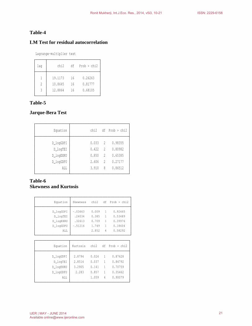
Table-4

LM Test for residual autocorrelation

3 12.8864 16 0.68105

2 10.8645 16 0.81777

1 19.1173 16 0.26263

lag chi2 df Prob > chi2

Lagrange-multiplier test

Table-5

Jarque-Bera Test

ALL 3.910 8 0.86512

D_logGDPU 2.606 2 0.27177

D_logEXRU 0.850 2 0.65385

D_logTEI 0.422 2 0.80982

D_logGDPI 0.033 2 0.98355

Equation chi2 df Prob > chi2

Table-6 Skewness and Kurtosis

ALL 2.852 4 0.58292

D_logGDPU -.51216 1.749 1 0.18604

D_logEXRU .32613 0.709 1 0.39976

D_logTEI .24034 0.385 1 0.53489

D_logGDPI -.03663 0.009 1 0.92465

Equation Skewness chi2 df Prob > chi2

ALL 1.059 4 0.90079

D_logGDPU 2.283 0.857 1 0.35462

D_logEXRU 3.2905 0.141 1 0.70759

D_logTEI 2.8514 0.037 1 0.84792

D_logGDPI 2.8794 0.024 1 0.87628

Equation Kurtosis chi2 df Prob > chi2



21

IMPACT OF THE GLOBAL FINANCIAL CRISIS ON THE EXPORT …ijeronline.com/documents/volumes/Vol 5 iss...

Documents

Transcript of IMPACT OF THE GLOBAL FINANCIAL CRISIS ON THE EXPORT …ijeronline.com/documents/volumes/Vol 5 iss...