Impact of Surrounding Land Uses on Surface Water Quality

by

Mark A. Elbag Jr.

A Thesis

Submitted to the Faculty

of the

WORCESTER POLYTECHNIC INSTITUTE

in partial fulfillment of the requirements for the

Degree of Master of Science

in

Environmental Engineering

by

____________________________________ Mark A. Elbag Jr.

May 2006

APPROVED: ____________________________________ Dr. Jeanine D. Plummer, Major Advisor ____________________________________ Dr. John Bergendahl, Advisor

ii

Abstract Source water protection is important to maintain public health by keeping harmful pathogens out of drinking waters. Non-point source pollution is often a major contributor

of pollution to surface waters, and this form of pollution can be difficult to quantify. This study examined physical, chemical, and microbiological water quality parameters that

may indicate pollution and may help to identify sources of pollution. These included measures of organic matter, particles, and indicator organisms (fecal coliforms and E.

coli). The parameters were quantified in the West Boylston Brook in Massachusetts, which serves as a tributary to the Wachusett Reservoir and is part of the drinking water

supply for the Metropolitan Boston area. Water quality was determined over four seasons at seven locations in the brook that were selected to isolate specific land uses.

The water quality parameters were first analyzed for trends by site and by season. Then, a correlation analysis was performed to determine relationships among the water quality

parameters. Lastly, ANOVA analyses were used to determine statistically significant variations in water quality along the tributary.

iii

Acknowledgements

I would like to thank Professor Jeanine Plummer who provided support and guidance through the year and a half of study. I would like to thank Karen Kosinski for

her assistance in the laboratory. I would like to thank Professor Sharon Long and Mike Tache for the analysis done in conjunction at the University of Massachusetts, Amherst.

And, I would like to thank The Department of Conservation and Recreation and Erin Ringer.

iv

Table of Contents

1.0 Introduction................................................................................................................... 1 2.0 Literature Review ......................................................................................................... 3

2.1 Source Water Management....................................................................................... 3 2.1.1 Surface Water Pollution..................................................................................... 3

2.1.1.1 Point Source Pollution ................................................................................ 4 2.1.1.2 Non-point Source Pollution ........................................................................ 5

2.1.2 Drinking Water Regulations .............................................................................. 5 2.1.2.1 Filtration Waiver for Surface Water Supplies ............................................ 7

2.2 Department of Conservation and Recreation............................................................ 7 2.2.1 DCR/MWRA Water System.............................................................................. 8 2.2.2 Watershed Protection ......................................................................................... 8

2.3 Watershed Monitoring ............................................................................................ 10 2.3.1 Land Use Surveys ............................................................................................ 10 2.3.2 Water Quality Monitoring................................................................................ 11

2.3.2.1 Physical Water Quality Monitoring .......................................................... 11 2.3.2.1.1 Temperature ....................................................................................... 11 2.3.2.1.2 Specific Conductance......................................................................... 11 2.3.2.1.3 Turbidity ............................................................................................ 13

2.3.2.2 Chemical Water Quality Monitoring ........................................................ 13 2.3.2.2.1 pH....................................................................................................... 14 2.3.2.2.2 Dissolved Oxygen.............................................................................. 14 2.3.2.2.3 Organic Carbon.................................................................................. 14 2.3.2.2.4 Measure of Organic Matter with UV254 ............................................. 16

2.3.3 Microbiological Water Quality Monitoring..................................................... 16 2.2.3.1 Fecal Coliforms and E. coli As Indicator Organisms ............................... 17 2.3.3.2 Microbial Source Tracking ....................................................................... 19 2.3.3.3 FC/FS Ratios............................................................................................. 19 2.3.3.4 Host Specific Organisms........................................................................... 19

2.3.3.4.1 Bifidobacteria..................................................................................... 19 2.3.3.4.2 Rhodococus coprophillus................................................................... 20 2.3.3.4.3 Coliphages.......................................................................................... 20

3.0 Methods ...................................................................................................................... 21 3.1 Experimental Design............................................................................................... 21

3.1.1 Sampling Locations ......................................................................................... 21 3.1.2 Sampling Dates ................................................................................................ 22 3.1.3 Sampling Protocol............................................................................................ 22 3.1.4 Transporting and Splitting Samples................................................................. 24

3.2 Laboratory Analytical Procedures .......................................................................... 24 3.2.1 Turbidity .......................................................................................................... 25 3.2.2 pH..................................................................................................................... 26 3.2.3 UV254................................................................................................................ 26 3.2.4 Particle Counts ................................................................................................. 26 3.2.5 Fecal Coliforms................................................................................................ 27

3.2.5.1 m-FC Agar ................................................................................................ 27

v

3.2.5.2 Buffered Water.......................................................................................... 28 3.2.5.3 Filtering..................................................................................................... 28

3.2.6 E. coli ............................................................................................................... 29 3.2.6.1 Nutrient Agar with MUG.......................................................................... 29 3.2.6.2 E. coli Enumeration .................................................................................. 29

3.2.7 Positive and Negative Controls for Fecal Coliforms and E. coli ..................... 30 3.2.8 Total and Dissolved Organic Carbon............................................................... 30

3.2.8.1 Standard Preparation................................................................................. 31 3.2.8.2 TOC/DOC Quantification......................................................................... 32

3.3 Statistical Analysis.................................................................................................. 32 3.3.1 Correlation Analysis ............................................................................................ 33

3.3.2 ANOVA Analysis ............................................................................................ 33 3.3.3 Binary Data Sets .............................................................................................. 34

4.0 Results......................................................................................................................... 35 4.1 Sampling Site Descriptions..................................................................................... 35 4.2 Sampling Dates ....................................................................................................... 42 4.3 Variations in Water Quality Parameters among Sampling Locations .................... 43

4.3.1 Chemical Water Quality Parameters by Site ................................................... 43 4.3.2 Particulate Matter by Site................................................................................. 47 4.3.3 Organic Matter by Site..................................................................................... 49 4.3.4 Indicator Organisms by Site............................................................................. 51

4.4 Variation in Water Quality Parameters by Season ................................................. 53 4.4.1 Chemical Water Quality Parameters by Season .............................................. 53 4.4.2 Particulate Matter by Season ........................................................................... 55 4.4.3 Organic Matter by Season................................................................................ 56 4.4.4 Indicator Organisms by Season ....................................................................... 57

4.5 Statistical Analysis.................................................................................................. 59 4.5.1 Correlation Analysis ........................................................................................ 59

4.5.1.1 Correlation Analysis with Stage Height ................................................... 63 4.5.2 ANOVA Analysis ............................................................................................ 63

4.5.2.1 ANOVA Site Analysis.............................................................................. 63 4.5.2.2 ANOVA Seasonal Analysis...................................................................... 65

4.5.3 ANOVA Analysis of the Binary Data Set ....................................................... 67 4.5.3.1 ANOVA Analysis of the Binary Data Set by Site .................................... 68 4.5.3.2 ANOVA Analysis of the Binary Data Set by Season ............................... 69

5.0 Conclusions and Recommendations ........................................................................... 71 5.1 Conclusions............................................................................................................. 71 5.2 Recommendations................................................................................................... 72

References......................................................................................................................... 73 Appendix A: Experimental Results .................................................................................. 78 Appendix B: ANOVA Analyses by Site........................................................................... 82 Appendix C: ANOVA Analyses by Season ..................................................................... 89 Appendix D: Binary ANOVA Analysis by Site ............................................................... 96 Appendix D: Binary ANOVA Analysis by Season ........................................................ 100

vi

List of Figures

Figure 1: Land Uses in the West Boylston Brook Subbasin............................................. 36 Figure 2: Sampling Locations in the West Boylston Brook Subbasin.............................. 37 Figure 3: Photograph of Site F.......................................................................................... 38 Figure 4: Photograph of Site E.......................................................................................... 38 Figure 5: Photograph of Site D ......................................................................................... 39 Figure 6: Photograph of Site C ......................................................................................... 40 Figure 7: Photograph of Site B ......................................................................................... 40 Figure 8: Photograph of Site A ......................................................................................... 41 Figure 9: Photograph of Sampling Location at Gate 25. .................................................. 42 Figure 10: Temperatures and Dissolved Oxygen Levels on October, 23 2005............... 44 Figure 11: pH and Conductivity on October 23, 2005..................................................... 46 Figure 12: Turbidity and Particle Counts on October 23, 2005....................................... 48 Figure 13: Organic Carbon and UV254 Absorbance Levels on October 23, 2005 ........... 50 Figure 14: Fecal Coliform and E. coli Concentrations on October 23, 2005 .................. 52 Figure 15: Temperature and Dissolved Oxygen Concentration at Gate 25 ..................... 54 Figure 16: Conductivity and pH at Gate 25 ..................................................................... 55 Figure 17: Turbidity and Particle Counts at Gate 25 ....................................................... 56 Figure 18: Organic Carbon Levels and UV254 Absorbance at Gate 25............................ 57 Figure 19: Fecal Coliform and E. coli levels at Gate 25.................................................. 58 Figure 20: Fecal Coliform and E. coli Levels at Site C ................................................... 59

vii

List of Tables

Table 1: Field Measurements........................................................................................... 23 Table 2: Laboratory Tests ................................................................................................ 25 Table 3: Working Standards for TOC/DOC Analysis ..................................................... 32 Table 4: Sampling Site Descriptions................................................................................ 35 Table 5: Sampling Date with the Season the Sampling Represents ................................ 43 Table 6: Dissolved Oxygen Ranges................................................................................. 45 Table 7: Conductivity Ranges.......................................................................................... 47 Table 8: Turbidity Ranges ............................................................................................... 49 Table 9: Total Organic Carbon Ranges ........................................................................... 51 Table 10: Fecal Coliform Ranges ..................................................................................... 53 Table 11: Number Data Points for each Water Quality Parameter and the Minimum

R-Values Needed Statistically Significant Correlation (95% Confidence Level) .... 60 Table 12: R-Values for Correlation Analysis on Water Quality Data .............................. 61 Table 13: Correlations between Water Quality Parameters.............................................. 62 Table 14: R-Values for each Water Quality Parameter Correlated with Stage Height .... 63 Table 15: Number of Data Points for the ANOVA Site Analyses ................................... 64 Table 16: P-Values for Each Water Quality Parameter According to Variations by Site 65 Table 17: Number of Data Points for the ANOVA Seasonal Analyses ........................... 65 Table 18: P-Values for Each Water Quality Parameter According to Variation by

Season ....................................................................................................................... 66 Table 19: Benchmark Pollution Levels............................................................................. 68 Table 20: P-Values for each Binary Water Quality Parameter According to Site

Variation ................................................................................................................... 69 Table 21: P-Values for each Binary Water Quality Parameter According to Seasonal

Variation ................................................................................................................... 70

1

1.0 Introduction

Much of the drinking water for the United States comes from surface water bodies

such as lakes and rivers. For public health reasons, it is very important that drinking water sources or public water supplies are kept clean and free of pollution. Surface

waters are vulnerable to pollution from their surrounding environment, and protection of surface waters is a complicated process that must often be done on a regional level.

Surface water bodies can be polluted from point source pollution as well as non-point source pollution. The latter of the two can be hard to locate, quantify, and/or

regulate. Locating non-point sources of pollution to surface water bodies is challenging because the sources may be located within the entire watershed area. Runoff that travels

over various land uses within a watershed is a major source of non-point source pollution. Through water quality monitoring and watershed land use surveys, public agencies work

to locate and eliminate non-point sources of pollution to source waters. The U.S. Environmental Protection Agency (EPA) oversees protection of water in

the United States, which includes protection of surface waters and public water supplies. More locally, the Massachusetts Department of Conservation and Recreation (DCR)

protects several water bodies in Massachusetts that serve as a public water supply for the Boston Metropolitan area. One of the reservoirs protected by the DCR is the Wachusett

Reservoir located in central Massachusetts. This reservoir has had some non- point source pollution problems in several specific watershed areas or subbasins. The West

Boylston Brook (WBB) watershed subbasin is one such area of the watershed that has had a history of pollution problems.

This study investigated the pollution problems in the WBB through physical, chemical, and biological water monitoring. Physical measurements included

temperature, specific conductance, turbidity, and particle counts. Chemical measurements included pH, dissolved oxygen, and organic carbon (total organic carbon,

dissolved organic carbon, and UV254 absorbance). Biological measurements included fecal coliforms and E. coli. Water quality parameters were measured at seven locations

over a period of thirteen months in the brook to aid in determining the quality of the

2

water and the possible sources of pollution to the brook. Analysis of the data was conducted to determine contamination sources to the brook.

This study also evaluated the usefulness of various water quality parameters for source water protection. The collected data were analyzed to assess correlations between

water quality parameters, and water quality differences among sampling sites and among seasons. Further analysis was carried out using a binary number system for several of the

water quality measurements. Recommendations are provided for determining what land uses are polluting the surface water and for selecting which water quality parameters are

most valuable for source water protection. The next chapter describes the current literature on federal and state programs for

monitoring and regulation, water quality parameters, and the affects of land uses on surface water quality. Chapter 3 discusses the methods used for collecting and analyzing

water quality data as well as statistical analyses conducted on the data. Finally, the results of this study are presented in Chapter 4, and the recommendations on the

usefulness of water quality indicators in monitoring surface waters are presented in Chapter 5.

3

2.0 Literature Review

Safe drinking water is essential for maintaining public health. Every effort should

be made to achieve the highest quality drinking water possible. Protection of water supplies from contamination is the first step in providing clean drinking water. Source

protection is one method of ensuring safe drinking water, and is used in conjunction with appropriate treatment and distribution procedures. For a source water protection program

to be effective, pollution problems or risks within a watershed need to be identified. This is accomplished through watershed monitoring, which consists of water quality

monitoring and land use surveys. This chapter provides background on source water protection strategies, regulations, land use impacts on water quality, and methods to

identify pollution sources in a watershed.

2.1 Source Water Management

Source water is untreated water from streams, rivers, lakes, or underground aquifers which is used to supply private wells and public drinking water systems (EPA,

2005j). Source water management consists of protecting and treating source water to obtain adequate drinking water for a population. Source waters are protected from

pollution as much as possible to reduce risks to public health. In addition, protecting a source water can be more economical than treating unprotected waters to obtain clean

drinking water. Source water protection programs also protect valuable ecosystems for fish, other aquatic species, and wildlife, as well as preserve the natural environment for

some recreational activities.

2.1.1 Surface Water Pollution

Surface water sources should be protected as much as possible from contamination by harmful pollutants. Potential pollutants include microorganisms,

inorganic chemicals, organic chemicals, and radionuclides (EPA, 2005d). Completely protecting source water may not be possible because pollutants from the atmosphere can

enter a surface water through precipitation, and contaminated ground water can introduce pollutants through recharge. However, limitations on land use around a surface water can

reduce contamination of surface waters from the watershed itself.

4

Surface waters can be polluted by industrial and municipal discharges as well as altercations to the natural environment, which may cause runoff of pollutants. Both

direct discharges and runoff can include human and animal waste. Human and animal feces may contain bacterial, viral, and protozoan pathogens as well as helminth parasites.

Failure to provide adequate protection and effective treatment for drinking water can expose the community to the risk of intestinal and other infectious diseases.

Surface water pollution is classified into two major categories: point source pollution and non-point source pollution. Non-point source pollution, often in the form

of runoff, comes from diffuse or scattered sources in the environment, while point source pollution comes from a defined outlet such as a pipe (EPA, 2005g). Non-point source

pollution may be difficult to identify and control while point source pollution can be identified easily.

2.1.1.1 Point Source Pollution

Point source pollution, such as pipe discharges, industrial outflows, tributaries, or

wastewater treatment plant outflows are relatively easy to define and regulate. The EPA regulates point source discharges throughout the United States with the National

Pollution Discharge Elimination System (NPDES) permitting program. The NPDES program, which was introduced in 1972, requires point source dischargers to obtain

permits from their state. This includes industrial and municipal dischargers, or any other facility that discharges wastewater to receiving water. The program greatly assists in the

control of point source pollutants of anthropogenic origin. NPDES permits specify the allowable flow rate of a discharge and the maximum concentration of specific pollutants.

The NPDES is an effluent based program which does not take into account the amount of pollutant that can safely be added to a specific water body without degrading that water.

Therefore, the amount of pollutant that is allowed from a discharger is not dependant upon the size of the water body or the number of other dischargers to the water body.

Another tool to protect surface waters is the calculation of a Total Maximum Daily Load (TMDL) of a surface water. A TMDL is the total amount of a pollutant that a

surface water can receive from all sources of pollution and still meet water quality standards. The Clean Water Act establishes the water quality standards for various

5

surface water uses (EPA, 2005k) The maximum load would be set differently if a water was used for drinking verses recreation (swimming and fishing), or for supporting aquatic

life. A TMDL is a water body quality based regulation, and may be more stringent than a NPDES permit alone.

2.1.1.2 Non-point Source Pollution

Non-point source (NPS) pollution is typically caused by rainfall or snowmelt

moving over or through the ground, picking up natural and human pollutants, and carrying those pollutants into surface waters. Pollutants include but are not limited to

excess fertilizers, herbicides, and insecticides from agricultural lands and residential areas; oil, grease, and toxic chemicals from urban runoff and energy production; sediment

from improperly managed construction sites, crop and forest lands, and eroding stream banks; salt from irrigation practices and acid drainage from abandoned mines; and

bacteria and nutrients from livestock, pet wastes, and faulty septic systems (EPA, 2005l). Non-point source pollution is a major problem for surface waters because it is

often times difficult to identify the source of the pollution. Therefore, control of non- point sources of pollution is problematic. Often times, land use surveys and groundwater

or surface water quality samples are the only ways of identifying where possible non-point sources may be located. NPS pollution is managed by states through watershed

protection programs, which are discussed further in Section 2.2.2.

2.1.2 Drinking Water Regulations

The EPA sets and enforces drinking water regulations in the U.S. Under the Safe Drinking Water Act, the EPA advocates a “multiple barrier” approach to drinking water

protection. The first part of the multiple barrier approach is source water protection. Source water protection includes assessing and protecting drinking water sources,

protecting groundwater wells, and protecting surface water collection systems. The second part of the multiple barrier approach involves water treatment conducted by

qualified operators. In addition, operators must ensure the integrity of distribution systems. Lastly, the multiple barrier approach requires water utilities to provide

information to the public on the quality of their drinking water (EPA, 2005h).

6

The EPA drinking water standards apply to all public water supplies. Public water supplies provide water for human consumption through at least 15 service

connections, or regularly serve at least 25 individuals. Public water systems include municipal water companies, homeowner associations, schools, businesses, campgrounds

and shopping malls (EPA, 2005h). There are two categories of drinking water standards: the national primary

drinking water standards and the national secondary drinking water standards. The national primary drinking water standards are legally enforceable standards that apply to

public water systems. Primary standards protect drinking water consumers by limiting the levels of specific contaminants that can adversely affect public health and are known or

anticipated to occur in water. The national secondary drinking water standards are non-enforceable guidelines regarding contaminants that may cause cosmetic effects (such as

skin or tooth discoloration) or aesthetic effects (such as taste, odor, or color) in drinking water. EPA recommends secondary standards to water systems but does not require

systems to comply (EPA, 2005h). Regulated contaminants can be grouped into three categories: non-carcinogens

(not including microbial contaminants) which cause adverse non-cancerous health effects, carcinogens, and microbial contaminants. The latter category includes protozoa,

viruses, and bacteria that cause adverse health effects (EPA, 2005h). Drinking water regulations set by the EPA include maximum contaminant levels (MCLs) and treatment

techniques. Maximum contaminant levels are set to minimize health risks while also considering the cost of treatment processes for removing contaminants. Microbial

contaminant MCLs are set at zero because ingestion of one protozoan, virus, or bacterium could cause illness.

Any public water supply that obtains water from a surface water is regulated by the Surface Water Treatment Rule (SWTR) which was first promulgated by the EPA in

1989. The SWTR requires disinfection and filtration for all public water supplies that use surface water or a ground water that is under direct influence of surface water as a source

(MDHHS, 2005). However, a filtration avoidance waiver can be granted to drinking water suppliers by the EPA if the surface water source meets specific quality

requirements (MDHHS, 2005). The SWTR has also been expanded over the years with

7

the additions of the Long Term 1 Enhanced SWTR (LT1 ESWTR), and Long Term 2 Enhanced SWTR (LT2 ESWTR).

2.1.2.1 Filtration Waiver for Surface Water Supplies

Surface water supplies which meet strict criteria for quality and protection may

apply for a filtration waiver under the SWTR. Systems which have a filtration waiver must continue to meet all MCL requirements, must disinfect the water, and must have the

capability of redundant disinfection in case of microbial water contamination. In addition, the EPA also requires a watershed control program which encompasses many

steps to minimize microbial contamination of the source water. To be allowed filtration avoidance, the source water protection programs must

characterize the watershed’s hydrology, physical features, land use, source water quality and operational capabilities. Programs must also identify, monitor and control both

human and natural activities that may deteriorate water quality. The watershed control program must also be able to control activities through land ownership or written

agreements (EPA, 2005m). To qualify for the SWTR filtration avoidance, source water must meet coliform

bacteria and turbidity requirements. Ninety percent of the samples taken from the source water must have fewer than 100 total coliform bacteria per 100 ml, and fewer than 20

fecal coliform bacteria per 100 ml of source water (EPA, 1991). The turbidity of the source water prior to disinfection must be less than 5 ntu (EPA, 1991).

More current legislation from the LT1 and LT2 ESWTRs have set more stringent guidelines for water treatment. The LT2 ESWTR contains regulations set to protect

against Cryptosporidium. The legislation calls for monitoring drinking waters for Cryptosporidium and many of the guidelines are based upon the levels of E. coli found in

a source water.

2.2 Department of Conservation and Recreation

The Massachusetts Department of Conservation and Recreation (DCR), formerly known as the Metropolitan District Commission (MDC), manages and protects the

drinking water supply for the communities in and around greater Boston. The Massachusetts Water Resources Authority (MWRA) treats and distributes the water to

8

communities in the Boston area. Greater Boston’s drinking water system has a filtration waiver from the EPA because of high source water quality and the watershed protection

provided by the DCR. Massachusetts has one of the largest source water systems in the world which serves nearly 2.5 million people in 46 different cities and towns throughout

the commonwealth (DCR, 2005b).

2.2.1 DCR/MWRA Water System

The source water system for the greater Boston area is made up of three different watersheds including the Quabbin Reservoir, Wachusett Reservoir, and Ware River

watersheds. The Quabbin Reservoir was built in the 1930’s by damming the Swift River with the Windsor Dam, which flooded four Massachusetts towns located in the Swift

River Valley. Hundreds of homes, businesses, a state highway, a railroad line and 34 cemeteries had to be moved out of the valley (DCR, 2005b). The reservoir has a volume

of 412 billion gallons of water, covers 39 square miles, and is 18 miles long. The reservoir is fed by a 95,000 acre watershed (DCR, 2005b).

The Wachusett Reservoir was built in 1906 by damming the Nashua River in Clinton, MA. The reservoir, with a volume of 65 million gallons, has a surface area a 6.5

square miles and a 110 square mile watershed feeding into it from 12 different Massachusetts towns (DCR, 2005e).

The Ware River is used to provide additional water to the Quabbin Reservoir. From the months of October to June when the Ware River waters are high, a portion of

the Ware River’s water is diverted into the Quabbin tunnel, and piped into the reservoir. The Ware River is fed by a watershed consisting of approximately 62,000 acres (DCR,

2005b).

2.2.2 Watershed Protection

The Massachusetts Department of Conservation and Recreation protects source water quality through several means. The Watershed Protection Act (WsPA) was created

by the Commonwealth of Massachusetts to protect drinking water sources, which includes the Quabbin Reservoir, Ware River, and Wachusett Reservoir, from pollution.

With the WsPA, the DCR has the ability to restrict activities in the watersheds in order to reduce non-point source pollution. Some of the strategies used by the DCR include land

9

acquisition, use of a buffer zone along surface waters, limitations on impervious surfaces, and restrictions on the use and storage of hazardous materials within the watersheds.

One method of protecting water quality is the use of buffer zones. The DCR places various restrictions on land uses within 400 feet of any surface waters, flooding

planes, or underground aquifers. The Watershed Protection Act defines two zones: the primary protection zone and the secondary protection zone. The primary protection zone

covers all areas within 400 feet of reservoirs and 200 feet of surface waters or tributaries. The secondary zone covers all areas within 200 and 400 feet of tributaries and surface

waters, on land within flood plains, over some aquifers, and within bordering vegetated wetlands (DCR, 2005a). Any alterations of land within the primary protection zone are

prohibited, and there are many restrictions on land uses and activities within the secondary zone.

The DCR not only protects the source water system through land use restrictions, but also through land acquisition. The DCR has acquired significant acreage throughout

the watersheds and continues to do so with the use of sophisticated computer models to identify the most sensitive land areas within the watersheds (DCR, 2005b).

Microbial and pathogenic contamination is partly controlled by restricting public access to the source waters and controlling some of the wildlife within the three

watersheds. Human and animal presence on watershed lands increases the risk of pathogens contaminating the source waters. Public access is limited on DCR land,

especially near any water intake structures. Swimming is not allowed in the reservoirs. Other human activities that may contribute to pathogen contamination include improper

disposal of fecal waste from dogs, horses, or any other domestic animals on watershed land.

Some species of wildlife need to be controlled by the DCR because of their proximity to intake structures or because they can transmit harmful pathogens to humans.

The animals that are targeted as threats to water quality are gulls, Canadian geese, ducks, beavers, muskrats and deer (DCR, 2005h). The goals of the wildlife control program are

to minimize the presence of waterfowl at the water intakes to reduce high coliform counts at intake structures; to eliminate muskrat and beaver from sensitive water zones and

zones near water intakes due to the harmful pathogens from the species; and to keep deer

10

populations at an appropriate number (DCR, 2005h). The main goal of the DCR’s wildlife control program is to keep pathogens from the getting into the water intake,

especially pathogens harmful to humans such as pathogens from beavers and a few other animal species.

2.3 Watershed Monitoring

In 1996, the Safe Drinking Water Act Amendments placed a renewed emphasis

on source water protection (EPA, 2005j). States were given access to funding and required to develop Source Water Assessment Programs (SWAP). The goals of SWAPs

are to identify potential threats to drinking water sources and initiate protection efforts. The four major elements of a SWAP are delineating or mapping source water assessment

areas, conducting an inventory of potential sources of contamination, determining the susceptibility of the water supply to harmful contamination, and releasing results of the

study to the public (EPA, 2005j).

2.3.1 Land Use Surveys

Land use surveys are useful for identifying possible sources of pollutants. Land use within a watershed is classified into several categories. An example of a few land use

classifications are industrial or commercial, farmland, and residential. If there are known pollutants in a water body, a land use survey of the watershed area could be

helpful in identifying where the pollutant or pollutants may have come from. Based on prior land use and water quality studies, certain land uses have been associated with

specific contaminants. Land use surveys also allow for a prediction of the risk of a pollutant entering the

water. When land is acquired for source water protection, it is important that the funds to acquire land are used in the most beneficial fashion. A land use survey of a watershed

would allow for the highest risk areas of land to be acquired. Land use surveys are an important tool in water quality monitoring and source

water protection, but a land use survey needs to be used in conjunction with water quality monitoring to be completely effective. Land use surveys may yield possible pollutant

threats, but water quality then needs to be tested to isolate true sources of pollution.

11

2.3.2 Water Quality Monitoring

Water quality monitoring can be used to protect source waters by identifying

pollutant levels and locations in a source water. Water quality monitoring is commonly done multiple times a year because water quality may change with season and with

weather events. Water quality can be monitored by measuring physical, chemical, or biological characteristics of the water.

2.3.2.1 Physical Water Quality Monitoring

Physical measurements consist of measuring water temperature, flow, specific

conductance, turbidity, and the condition of stream or lake banks. Physical characteristics are often related to chemical parameters. For example, eroding stream

banks may be the cause of high suspended solids or low flow may be the cause of low dissolved oxygen content. Three measurable physical parameters that were measured in

this study include temperature, specific conductance, and turbidity.

2.3.2.1.1 Temperature

The temperature of the water may affect both chemical and biological water characteristics. Rates of many biological and chemical processes vary with temperature.

Biological water quality may vary with temperature due to varying species survival rates in different temperatures.

A chemical characteristic that varies with the temperature of the water is dissolved oxygen content. The saturation value of dissolved oxygen in water is inversely

related to the temperature of the water. Therefore, in temperate climates, levels are typically higher in the winter and lower in the summer.

2.3.2.1.2 Specific Conductance

Specific conductance or conductivity of water is a measure of the ease with which

an electrical current can pass through water. A high conductivity is a result of the presence of inorganic dissolved solids that carry a charge. Some examples of dissolved

solids that are able to carry a charge are iron, calcium, chloride and sulfate. The specific conductance of a surface water can be affected by both natural and anthropogenic factors

in the watershed.

12

The natural conductivity of a surface water body that has not been affected by human activities depends mainly on the geography of the area. The conductivity of

surface water can vary depending upon the type of rock or soil that the water has come in contact with. Water that has come in contact with granite bedrock tends to have a low

conductivity and water that has come in contact with clay soils tends to have a high conductivity.

Other natural variations in surface water conductivity can be caused by the type or amount of biological activity in a surface water (Copertino et al., 1998). For example, a

high rate of decay of organic matter by biological processes can affect the conductivity of the water. Degradation of plant matter increases the dissolved solids as well as the

conductivity in the water. Therefore, seasonal changed in biological activity may have an effect on the seasonal trends of conductivity levels.

The specific conductance of surface water is also influenced by human activities within a watershed. Pollutants that enter a surface water through runoff may raise or

lower the conductivity of a surface water. Organic compounds such as oil or alcohol lower the conductivity of water because they lack the ability to carry a charge. Areas

with a high percentage of impervious surfaces, such as urban areas, can yield runoff containing oils that may lower the conductivity of a nearby surface water (Mehaffey et

al,. 2005). However, Detenbeck et al. (1995) found that the majority of high concentrations of inorganic suspended solids occurred in the early spring in an urban

wetland which raised the conductivity. Other human activities in a watershed that may raise the conductivity of surface

waters include agricultural and residential land uses. During snowmelt periods, it has been shown that surface waters surrounded by agricultural lands have a higher specific

conductivity when compared to other land uses (Detenbeck et al., 1995). A failing septic system near a surface water body could raise the conductivity of that surface water due to

the presence of chloride, phosphate, and nitrate. Even a properly working septic system can affect the conductivity of nearby surface water. For example, New England area

homes with septic systems to treat wastewater often times have wells to provide drinking water. Water coming out of a well from bedrock often has a low conductivity. This

13

water may eventually be discharged to shallow ground water or surface water via septic system, affecting the conductivity of the receiving water (Burns et al., 2005).

2.3.2.1.3 Turbidity

Turbidity is a measure of the amount of suspended solids in a surface water.

Suspended solids include soil particles, algae, and microbes (EPA, 2005n). These substances enter into a water body through non-point source pollution, such as soil

erosion and urban runoff, and through processes within the water body, such as algal growth.

Turbidity levels in surface waters have been found to vary due to variations in precipitation and the percentage of impervious surface in a watershed. Long and

Plummer (2004) found turbidity levels in a small stream to vary with changes in precipitation. Volk et al. (2002) found that turbidity levels in a stream could increase by

as much as 300 fold during or following precipitation events. High turbidity levels in surface waters have been linked to high percentages of

impervious surfaces within a watershed caused by sediment loading from runoff and erosion. (Mehaffey et al., 2005; Nelson and Booth, 2002) In contrast, Shoonover et al.

(2005) found that during baseflow, turbidity concentrations were lower within watershed with higher percentages of impervious surfaces. Additionally, during typical storm

events, urban watersheds seemed to have similar turbidity as rural watersheds. The differing relationships between turbidity levels and land use may be due to the specific

watersheds included in each study. However, all of the studies were consistent in finding higher turbidity levels is surface water during periods with higher stream flow or

precipitation levels.

2.3.2.2 Chemical Water Quality Monitoring

Chemical water quality parameters may be used to indicate sources of pollution or be linked to other physical or biological water quality parameters. Chemical monitoring

in this study consisted of measuring pH, dissolved oxygen concentration, total and dissolved organic carbon levels, and UV254 absorbance.

14

2.3.2.2.1 pH

pH, which is a measure of the concentration of free H+ ions, is affected by acid

rain, surrounding rock formations, and certain wastewater discharges. Most fresh water aquatic species prefer a pH range of 6.5 to 8.0 (EPA, 2005n). Certain types of organisms

prefer different ranges of pH; if the pH is high or low it will change the types of organisms found in a surface water. A low pH can also allow toxic elements and

compounds to become mobile and available for uptake by organisms (EPA, 2005n).

2.3.2.2.2 Dissolved Oxygen

Dissolved oxygen (DO) enters a water body from the atmosphere and from oxygen producing plant life living in the water. The atmosphere is made of

approximately 20 percent oxygen or 200,000 ppm; typical oxygen levels in surface waters are below 10 ppm (Department of Wildlife and Fisheries Sciences, 2005).

There are many factors that influence the amount of DO in a surface water. Oxygen is transferred from the atmosphere into moving waters (streams and rivers) at a

higher rate than still waters, such as lakes. Water at a colder temperature also has a higher saturation level of dissolved oxygen than water at a warmer temperature. In

addition, water at a lower altitude has a higher saturation level than water at a higher altitude. The turbidity of a surface water can also affect DO levels. High turbidity in

surface water can reduce the level of DO by raising the water temperature and lowering photosynthesis due to the absorption of sunlight by suspended solids.

DO levels can provide information on the concentration of oxygen demanding pollutants that may be entering a surface water via point and non-point sources. Oxygen

is consumed by microorganisms as they degrade organic matter in a water, which reduces the DO concentration. These oxygen demanding substances may arise from farmland

runoff, urban runoff and septic systems. In particular, fertilizers, animal waste (livestock or wildlife), and human waste contribute to the oxygen demand.

2.3.2.2.3 Organic Carbon

Organic carbon is found naturally in surface water but may also be affected by

human activities. The level of organic carbon in a surface water is related to various characteristics of a watershed including land use, seasonal temperatures, and the amount

15

of precipitation a watershed receives. Natural organic carbon originates from plant life in or around the surface water and from soil runoff. Organic carbon levels can be measured

in terms of total organic carbon (TOC) or dissolved organic carbon (DOC). TOC levels in surface water have been shown to be dependent on the amount of

erosion entering a surface water. The type of soil that is eroding into a surface water will dictate how much the erosion will effect the TOC content. A study in the Rhode Island

area found the top 1 cm of forest land soil contained 4.3% organic carbon and the top 1 cm of soil in cropland contained 0.87% organic carbon (Correll et al., 2001). Correll et

al. (2001) indicates that erosion from croplands will raise the TOC levels more than the same amount of eroded soil from forestlands.

Erosion, which affects the amounts of TOC, is affected by land use and levels of precipitation. The highest fluxes in TOC occur in cropland areas rather than upland

forested areas (Correll et al., 2001). A flux in TOC levels indicates the source or the TOC is erosion due to precipitation events. According to Correll et al. (2001),

precipitation variations can account for 54-66% of the variation in annual TOC fluxes in a small single land use watershed, and TOC in surface waters near cropland and forested

land can be 3 to 5 times higher in a wet year than a dry year. Along with the levels of TOC, the levels of DOC have also been found to increase

with increased precipitation (Volk et al., 2002; Correll et al., 2001). Correll et al. (2001) found that 21-43% of the variation in concentration of DOC can be linked to discharge in

a mixed use watershed, and Volk et al. (2002) found that DOC concentration could increase by as much as 3 fold when discharge also increased by 3 fold in a small stream.

Although, TOC in surface waters adjacent to cropland is strongly related to the amount of runoff discharged, but DOC concentrations were not correlated with the watershed

discharge (Correll et al., 2001). Soil erosion is not the only contributor to organic carbon in surface waters.

Correll et al. (2001) found TOC concentrations to be significantly higher from upland forest than from other watershed land uses during low flow periods. These levels

indicate that near croplands the amount of TOC in a surface water is dependent upon the amount of eroded soil entering the surface water, but upland forested areas have high

levels of TOC that are not completely dependent upon soil erosion.

16

Flow and stream characteristics can affect DOC levels. In wetland areas surface waters with continuous flow were found to have lower dissolved organic carbon than

wetlands without continuous flow (Detenbeck et al., 1995). In an upland forested watershed, watershed discharge was linked to the concentration of TOC present as DOC,

and TOC concentrations were not linked to watershed discharge (Correll et al., 2001). There were some predominant trends between seasonal changes and the amount

of organic carbon in a surface water. Correll et al. (2001) found a strong correlation between TOC and mean temperature for the summer and winter season; with higher

temperatures in both seasons there were higher TOC concentrations (Correll et al., 2001). In addition, TOC concentrations were found to be higher from upland forest areas than

croplands in the fall season (Correll et al., 2001). TOC concentrations were also found to be lower during snowmelt periods than during other spring sampling periods (Detenbeck

et al., 1995; Correll et al., 2001), and DOC was higher in surface waters surrounded by agriculture than surface waters surrounded by any other type of land uses including

urban, residential, and forest land during snowmelt periods (Detenbeck et al., 1995).

2.3.2.2.4 Measure of Organic Matter with UV254

Some dissolved organic compounds in water absorb ultraviolet light. Therefore, measurement of ultraviolet light absorption at a wavelength of 254 nanometers (UV254) is

a surrogate for organic matter concentration. For example, Volk et al. (2002) found that levels of UV254 increase during or after precipitation events in streams and fluctuate in

correlation with dissolved organic carbon levels. However, UV254 had a higher level of variation than DOC (Volk et al., 2002).

2.3.3 Microbiological Water Quality Monitoring

Microbiological water quality monitoring consists of measuring the concentration

of microorganisms in a water body. Microorganisms of interest in surface water sources include bacteria, viruses, protozoa, and indicator organisms. Indicator organisms are

used to indicate the presence of other potentially harmful pathogens. Two microorganisms that are commonly used for surface water quality testing are fecal

17

coliforms and E. coli. The presence of fecal coliforms and E. coli indicates contamination of a surface water from human or animal waste.

2.2.3.1 Fecal Coliforms and E. coli As Indicator Organisms

An indicator organism is an organism that can provide information about the

health of a water body through the organism’s presence, condition, or numbers (EPA, 2005b). For surface waters, total colifoms, fecal coliforms and E. coli are used to

indicate the possible presence of harmful pathogens derived from human or animal waste. Some harmful pathogens of concern in source waters include Cryptosporidium, Giardia,

and E. coli O157: H7 (not all E. coli are harmful). An ideal indicator organism should be non-pathogenic, rapidly detected, easily

enumerated, and have survival characteristics that are similar to any harmful pathogens of concern. For assessing public health risk, indicator organisms include fecal colifoms and

E coli, which are normally found in the intestines and feces of humans, livestock, and wildlife. These organisms are relatively easy to detect and the enumeration process is

relatively inexpensive (Meays et al., 2004). There are two problems with using indicator organisms. First, it is difficult to

identify the source of the contamination. Second, it is not possible to know if bacterial contamination found in a source water indicates the presence of pathogens harmful to

humans. If fecal coliforms are found in source water, it may be difficult to identify whether the contamination is coming from wildlife, farmland, or septic systems. It is also

not possible to know from just testing for fecal coliforms if there are harmful pathogens present at all. The fecal material must come from an infected animal or human in order

for harmful pathogens to be present. There have been many links between different land uses and the amount of total

coliforms, fecal coliforms, and E. coli found in nearby surface waters. High fecal coliform counts have been positively related to urban development, agriculture, and the

amount of erodible soils (Mehaffey et al., 2005). High coliform counts are not only dependent on the total area of a particular land use within a watershed, but also on the

amount of precipitation that the watershed recieved in previous days (Mehaffey et al., 2005; Stukel et al., 1990).

18

Urban land use and agricultural land use seem to yield the highest concentrations of fecal coliforms in nearby surface waters (Mallin et al., 2000; Mehaffey et al., 2005;

Shoonover et al., 2005). Agricultural land use yields high levels of fecal coliforms depending upon the amount of agricultural debris that can erode into surface waters. A

high percentage of agriculture on very steep slopes adjacent to a surface water yields very high counts of fecal coliforms (Mehaffey et al., 2005). Vegetative strips or buffer zones

have been found to reduce nutrient loadings to surface waters from agricultural land use, but fecal coliform counts were not reduced (Fajardo et al., 2001).

In urban watersheds, a strong correlation exists between the percent impervious surface in the watershed and mean fecal coliform levels in suface waters (Shoonover et

al,. 2005; Young and Thackston, 1999). Mallin et al. (2000) also found a similarly strong correlation between population density and mean fecal coliform levels in surface waters.

Fecal coliforms are consistently higher during both base flow and high flow periods in urban watersheds compared to other land uses (Shoonover et al,. 2005).

The number of domestic animals in an urban watershed may be another cause of elevated fecal coliform levels (Mallin et al., 2000; Young and Thackston, 1999). Young

and Thackston (1999) found that high levels of fecal coliforms and E. coli in urban watersheds were the result of animal sources rather than human. They also found that

fecal coliform counts from septic systems in surface waters of an urban watershed were negligible in comparison to other sources of fecal coliforms.

Fecal coliforms levels can be affected by various physical and chemical parameters of a surface water. Total coliform, fecal coliform and E. coli levels may be

lower in surface waters with harsh living conditions for the organisms. The die off rate for the organisms can be accelerated, thus yielding possible lowered concentrations by

cold temperatures in the winter or extreme pH levels. In an urban watershed, fecal coliform levels were much higher in the summer than in the winter (Young and

Thackston, 1999). Turbidity is another surface water characteristic that may affect the levels of coliforms. Mallin et al, (2000) found that coliforms have a much longer

survival rate when in association with suspended solids. High levels of fecal coliforms were correlated with high levels of suspended solids in the Chesapeake Bay.

19

2.3.3.2 Microbial Source Tracking

Microbial source tracking (MST) is a way of identifying the source of

microorganisms in a watershed. By determining the pollutant source, an assessment can be made on the risk of pathogen contamination. There are many different methods of

microbial source tracking including comparison of fecal coliform concentrations to fecal streptococci levels, identifying host specific organisms, genotypic analyses, antibiotic

resistance analyses, and chemical identification. The following sections discuss the first two MST tools.

2.3.3.3 FC/FS Ratios

One form of microbial source tracking consists of determining the ratio of fecal

coliforms verses fecal streptococci, or the FC/FS ratio. Initially it was thought that a ratio of > 4.0 would indicate human pollution and < 0.7 would indicate non-human pollution

because observations had been made that human feces contained higher fecal coliform counts and animal feces contains higher levels of fecal streptococci (Scott et al., 2002).

This method of microbial source tacking has been proven unreliable due to varying survival rates of fecal streptococci (Scott et al., 2002).

2.3.3.4 Host Specific Organisms

Another form of microbial source tracking is finding bacteria that are present only

in the intestines of specific species or host specific organisms. A valuable host specific organism for source water protection is an organism that is either human specific or

animal specific and that can survive in the environment for a certain period of time. Three host specific organisms that may be used for source water protection are strains of

Bifidobacteria, Rhodococcus coprophilus, and coliphages.

2.3.3.4.1 Bifidobacteria

Strains of Bifidobacteria can be used as an indicator of human contamination in a source water. These bacteria are a major part of the human intestine, are rarely found in

animals (Scott et al., 2002), and certain strains of Bifidobacteria are only found in humans (Gavini et al., 1991). Bifidobacteria have not been found in unpolluted

environments such as springs, uncontaminated soil, or garden compost (Evison et al.,

20

1975). Differentiation is done to determine human strains on the basis of sorbitol fermentation (Mara et al., 1983). The two more prevalent human strains include

Bifidobacterium adolescentis and B. breve (Mara et al., 1983).

2.3.3.4.2 Rhodococus coprophillus

Strains of Rhodococcus coprophilus can be used as indicators of animal contamination, specifically livestock. Rhodococcus coprophilus is found in the feces of

farm animals (cattle, chickens, ducks, geese, horses, pigs, sheep, and turkeys) and in waters polluted by fecal material from these sources (Finlay et al., 1998). Two

successful source tracking studies have shown that the presence Rhodococcus

coprophilus can indicate grazing animal fecal contamination (Long et al., 2003; Long et

al. 2004).

2.3.3.4.3 Coliphages

A group of coliphages, F+RNA coliphages, have been the most widely researched coliphages for microbial source tracking (MST) applications. F+RNA coliphages are a

group of icosahedral phages which are morphologically similar to several human enteric virus groups, and thus have been proposed as indicators of enteric viruses (Sinton et al.,

1998). Furthermore, it was demonstrated through serotyping and genotyping that the majority of F+DNA coliphage isolate M13 were from domestic wastewater sources,

making it a possible human-specific viral indicator (Long et al., 2005).

21

3.0 Methods

The main goal of this project was to assess water quality in the West Boylston

Brook as well as to determine what water quality parameters should be used to indicate pollution. Seven sampling locations were chosen in the West Boylston Brook to

distinguish several different land uses in the watershed sub-basin. This chapter provides information on the sampling protocol. Second, this chapter discusses the analytical

procedures used for measuring each water quality parameter. Lastly, the chapter details how statistical analyses were performed on the water quality parameter data.

3.1 Experimental Design

Water quality can be assessed through physical, chemical, and microbiological

characteristics. Water quality can vary due to human or animal pollution, climate, and watershed characteristics. Sources of pollution from human activities can be determined

through measurement and analysis of several water quality parameters. This type of watershed monitoring is useful for development of source water protection programs.

The West Boylston Brook (WBB) watershed is a sub-basin watershed located in the Wachusett Reservoir watershed in Central Massachusetts. The Wachusett Reservoir

is one of the reservoirs which provides drinking water to Boston and the surrounding communities. The West Boylston Brook sub-basin watershed is one of the most

developed and most polluted sub-basin watersheds in the Wachusett Reservoir watershed. The WBB has historically had high levels of fecal coliforms and high turbidity levels.

3.1.1 Sampling Locations

Seven sampling locations were chosen along the WBB to determine possible

sources of pollution to the brook. The first site, Gate 25, is the sampling site used by the Department of Conservation and Recreation (DCR) near the confluence of the brook and

reservoir. This site as well as six other upstream locations were chosen based on surrounding land uses and isolation of potential pollution sources.

The six upstream sampling sites were lettered A thru F. Gate 25, Site A, Site B, Site D and Site E were all located in the main channel of the WBB. Sites C and F were

located in two other natural channels that feed into the main channel of the WBB. All of

22

the sampling locations were no more than approximately a half mile upstream of the reservoir. Detailed descriptions of the site locations and characteristics are provided in

the Results Chapter.

3.1.2 Sampling Dates

Sampling was done approximately once a month from February 2005 to February 2006. A total of ten sampling events were completed over these 13 months. Sampling

events included both wet and dry weather conditions. Two of the sampling events were completed during rain events (in May 2005 and October 2005). Sampling was done

during all four seasons. There were 3 winter sampling events between December 21st and March 21st; 2 spring sampling events between March 21st and June 21st; 3 summer

sampling events between June 21st and September 21st; and 2 fall sampling events between September 21st and December 21st. The exact sampling dates and the

precipitation conditions for those sampling events are provided in the Results Chapter.

3.1.3 Sampling Protocol

Sampling was done at the same time of day (mid morning) each sampling trip. Samples were taken from the most downstream site first and continued up to the most

upstream site. Sampling in this manner ensured that downstream water quality was not altered due to disturbances of upstream sites when sampling.

The first step in the sampling process was to note flow conditions, any changes in surrounding wildlife or human activity, the location that the sample was taken from, and

the time the sample was taken. At Gate 25, the flow was further characterized by recording the stage at a stage station located at the site. Next, the water sample was

collected directly from the stream. Samples were collected using either a 1 liter or a 4 liter sterilized bottle. If the

flow was deep enough, samples were taken directly with a 4 liter sterilized high density polypropylene (HDPP), Nalgene, wide mouth screw capped bottle (Nalge Nunc

International, Rochester, New York). If the flow was not deep enough, the sample was collected with a 1 liter sterilized high density polypropylene (HDPP), Nalgene, wide

mouth screw capped bottle (Nalge Nunc International, Rochester, New York) and then poured into the 4 liter bottle multiple times to fill the larger bottle. The sampler wore

23

rubber gloves sprayed with ethanol. Holding the bottom of the sample bottle, the mouth of the bottle was faced directly upstream and submerged into the middle of the stream to

mid-depth or at the water surface if the flow was too shallow to obtain mid-depth samples. While taking the water samples, it was important not to disturb anything

upstream of the sampling bottle or any of the sediments in the area from which the sample was taken. The full 4 liter sample bottles were then taken back to the car and

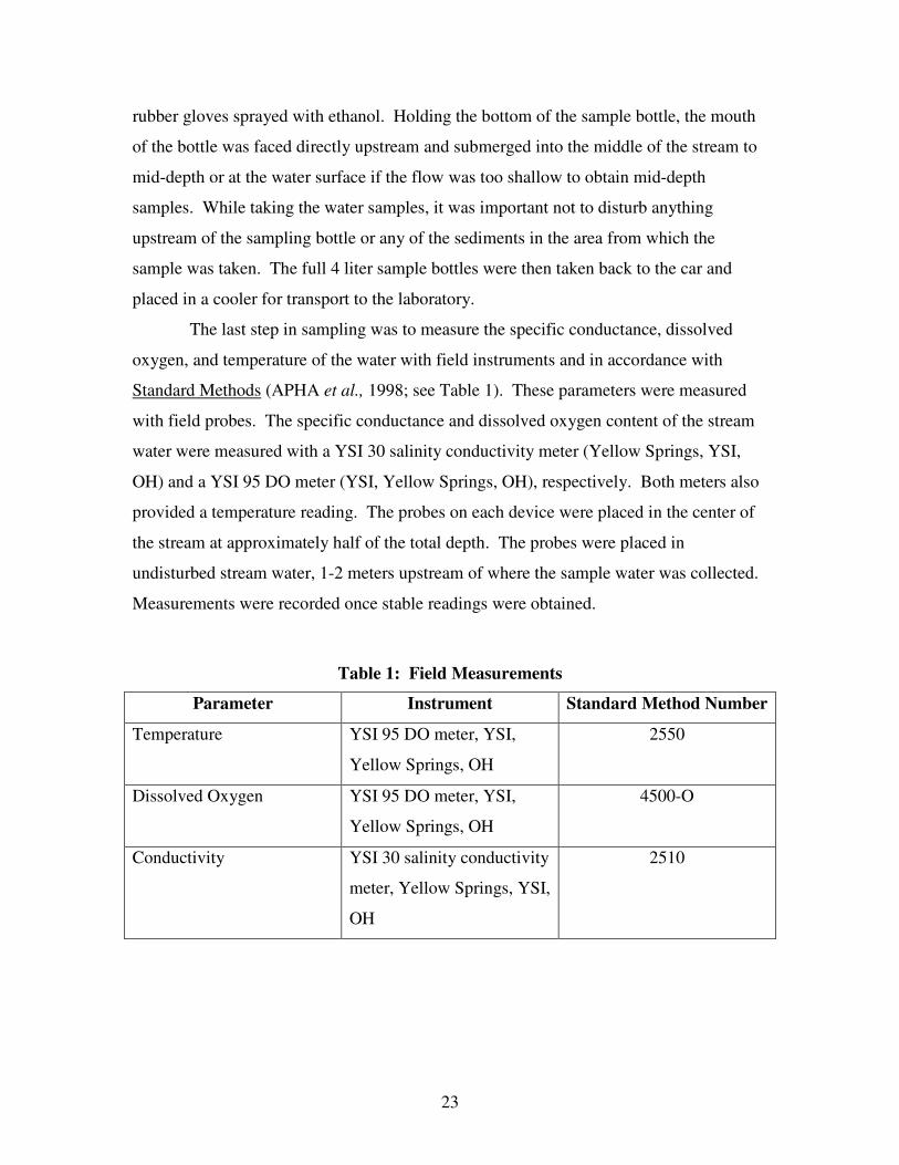
placed in a cooler for transport to the laboratory. The last step in sampling was to measure the specific conductance, dissolved

oxygen, and temperature of the water with field instruments and in accordance with Standard Methods (APHA et al., 1998; see Table 1). These parameters were measured

with field probes. The specific conductance and dissolved oxygen content of the stream water were measured with a YSI 30 salinity conductivity meter (Yellow Springs, YSI,

OH) and a YSI 95 DO meter (YSI, Yellow Springs, OH), respectively. Both meters also provided a temperature reading. The probes on each device were placed in the center of

the stream at approximately half of the total depth. The probes were placed in undisturbed stream water, 1-2 meters upstream of where the sample water was collected.

Measurements were recorded once stable readings were obtained.

Table 1: Field Measurements Parameter Instrument Standard Method Number

Temperature YSI 95 DO meter, YSI,

Yellow Springs, OH

2550

Dissolved Oxygen YSI 95 DO meter, YSI, Yellow Springs, OH

4500-O

Conductivity YSI 30 salinity conductivity meter, Yellow Springs, YSI,

OH

2510

24

3.1.4 Transporting and Splitting Samples

The samples were transported to the laboratory in the 4 liter HDPP bottles. The

bottles were placed in coolers with ice packs and a thermometer, which was used to verify transportation temperatures. Samples were split at the DCR laboratory in West

Boylston, MA directly after the last sample had been collected. The 4 liter bottles were inverted 20 times and this water was used to fill several smaller sterilized bottles

aseptically. For the analyses conducted at WPI, a one liter HDPP bottle was filled with sample water and placed back in the cooler with ice and a thermometer to be brought to

the laboratory at WPI. Remaining sample water was used for analyses at the University of Massachusetts laboratory.

3.2 Laboratory Analytical Procedures

The water characteristics that were measured at Worcester Polytechnic Institute in

the Environmental Engineering Laboratory are shown in Table 2. They include turbidity, pH, UV254, particle counts, fecal coliforms, E. coli, total organic carbon and dissolved

organic carbon. The samples were split upon arrival to the Worcester Polytechnic Institute Water Laboratory. Each bottle was thoroughly mixed, and sample water from

each site was poured aseptically from the 1 liter bottle into a 250 ml Nalgene, wide mouth screw capped bottles (Nalge Nunc International, Rochester, New York). The

sample water in the 250 ml bottle was used for pH, turbidity, UV254, TOC, DOC, and particle counts. Sample water remaining in the 1 L bottle was used for fecal coliforms

and E. coli. Aseptic conditions were maintained for these latter two analyses.

25

Table 2: Laboratory Tests Parameter Instrument Standard Method Number

Turbidity 2100N, Hach Company, Loveland, CO

2130

pH AB15, Fisher Scientific, Pittsburgh, PA

4500-H+

UV254 Cary 50, Varian, Palo Alto, CA

5910

Particle Count PC 2400 PS, Chemtrac

Systems Inc., Norcross, GA

2560

Dissolved Organic Carbon TOC-5000A, Shimadzu,

Colombia, Maryland

5510

Total Organic Carbon TOC-5000A, Shimadzu 5510

Fecal Coliforms not applicable 9222 D

E. coli not applicable 9222 G

3.2.1 Turbidity

The turbidity was measured using a Hach Model 2100N Laboratory Turbidimeter, (Loveland, CO) and in accordance with Standard Method 2130 (APHA et al., 1998).

Sample water from each site was poured into a clean, oiled turbidity vial after the sample bottle had been inverted several times. The turbidity vial was filled to the white line,

gently inverted several times, and placed into the turbidimeter (making sure to align the white arrow on the sample cell to the white line on the turbidimeter). A measurement

was obtained by waiting 15 seconds, watching the digital readout on the turbidimeter for 30 seconds and determinining an average reading. Two replicate measurements were

recorded for each sample. The turbidimeter was calibrated every 4 months with Stabl Cal Calibration standards of less than 0.1, 20, 200, 1000, and 4000 ntu (Hach Calibration

Standards Catalog Number 226621-05).

26

3.2.2 pH

The pH of the sample water was measured with a Fisher Scientific AB15 pH

meter (Pittsburgh, PA) in accordance with Standard Method 4500-H+(APHA et al., 1998). Sample water was poured into a small clean beaker from the 250 ml sample bottle

after inverting several times. The pH meter was calibrated before use with 4, 7, and 10 pH buffers. The pH probe was then placed in the sample and the value read from the

digital readout of the calibrated pH meter.

3.2.3 UV254

The absorbance of UV light at a wavelength of 254 nm was measured with a Varian Cary 50 Spectrophotometer (Palo Alto, CA) in accordance with Standard Method

5910 (APHA et al., 1998). Sample water from each site was prepared by filtering through a glass fiber filter (Whatman GF/F filter with 0.7 µm retention). First, the filters

were pre-washed with 20-30 ml of E-pure water. Then the sample was filtered. The first 5-10 ml of the sample was discarded, and next 10 ml was filtered into an acid washed 40

ml glass vial. From the 40 ml glass vial, the sample water was transferred into a Varian 10 mm, rectangular stoppered quartz spectrophotometer cell (Palo Alto, CA). The

spectrophotometer cell was pre-washed with E-pure water and wiped with a Kimwipe. The spectrophotometer cell was then filled with filtered sample water and inserted into

the spectrophotometer which yielded a digital readout. Duplicate measurements were recorded for each sample (emptying and cleaning the spectrophotometer cell between

readings). Two samples of E-pure water were measured to serve as zero readings. The average zero reading was subtracted from each sample reading to provide the true

absorbance.

3.2.4 Particle Counts

Particle counts were measured using a Chemtrac Systems PC 2400 PS Particle Counter with Grabbit 311 Software (Chemtrac Systems Inc, Norcross, GA). The

software was set up to purge with 25 ml of sample and then count particles in two subsequent 50 ml volumes of sample. The particle size intervals that the counter was set

up to measure were: 2-3, 3-4, 4-5, 5-6, 6-7, 7-8, 8-9, 9-10, 10-15, 15-20, 20-30, 30-40,

27

40-50, 50-75, 75-100, and 100 µm and greater. E-pure water (125 ml) was run through the instrument in between samples to ensure no carry-over.

The particle counts were done by first testing the port between the computer and the particle counter. The software program settings were then downloaded to the particle

counter from the computer. Next, the flow rate of the particle counter was adjusted to 100 ml per minute. This was done using a graduated cylinder and stopwatch, and

adjusting the flow rate as needed. To analyze the samples, the correct “tag name” was selected for the sample, and

the counter started by pressing the start button. After each sample, the data was saved. An E-pure sample was run between each sample to assure complete flushing of the

particle counter. After all samples were analyzed, the data were uploaded back to the computer and saved in MS Excel 4.0.

3.2.5 Fecal Coliforms

Fecal coliforms were measured in accordance with Standard Method 9222D, the

membrane filtration technique (APHA et al., 1998). This method involves filtering a volume of the sample, placing the filter on a Petri dish with nutrient media and allowing

time for bacterial colonies to grow. Sterile conditions were maintained throughout this analysis. Ideally, Petri dishes have 20-60 colonies per plate. To achieve this count range,

three or four different volumes of water were filtered depending upon previous levels of fecal coliforms and weather conditions on the particular sampling date.

3.2.5.1 m-FC Agar

Fecal coliform colonies are incubated on Petri dishes with m-FC agar (Difco #

267720, Sparks, MD). To prepare the agar, 52 grams of the agar was suspended in 1 liter of E-pure water in a sterile Erlenmeyer flask. The agar was heated to boiling and allowed

to boil for 1 minute with stirring. Then 10 ml of a 1% rosolic acid (prepared by dissolving 0.1 g of stock rosalic acid in 10 ml of 0.2 N NaOH) was then added to the

agar. The agar was boiled for another minute. The agar was then cooled in a water bath to 47 degrees Celsius.

Once the agar was cooled to 47ºC, 5 to 6 ml of the agar was dispensed into 50 x 9 mm Petri dishes and allowed to solidify. The Petri dishes containing solidified agar were

28

stored upside down at 4ºC in sealed plastic bags for a maximum of two weeks. The pH of the agar was checked on two plates to assure that it was 7.4 ± 0.2. The night before

using the plates, they were warmed in the 35ºC incubator.

3.2.5.2 Buffered Water

Buffered water is a solution that neither prohibits nor enhances growth of microorganisms. The buffered water is used for dilution of sample water as well as

washing the filter apparatus. Buffered water is made by diluting 1.25 ml of stock phosphate buffer and 5 ml of of stock magnesium chloride up to 1 L of E-pure water.

The stock magnesium chloride was made by dissolving 20.275 g of MgCl2·6H2O to a total volume of 250 ml of E-pure and the stock phosphate buffer was made by suspending

8.5 g of KH2PO4 up to 125 ml of E-pure.

3.2.5.3 Filtering

A filtration apparatus was assembled including a vacuum pump, filtration manifold, collection flask, and 47 mm filter funnels. First, flamed tweezers were used to

transfer a sterile 0.45 µm gridded membrane filter (Millipore Corp., Billerica, MA) onto the sterile filter tower apparatus (with the gridded side facing upwards). The filter towers

were pre-filled with 10 ml of buffered water for any water sample volumes that were below 10 ml. The water sample was then taken directly from the sample bottle after

inverting it three times and transferred into the filter tower. The vacuum pump was turned on and the tower was washed with buffered water from a squeeze bottle. Once the

water was filtered through the membrane, the vacuum pump was turned off. The filter paper was lifted with sterile tweezers and placed into a labeled Petri dish on top of the m-

FC agar, ensuring that the paper was in contact with the agar media. The filter tower was then washed with buffered water and the filtration steps were repeated.

Three replicate Petri dishes were prepared for each volume filtered, and 3 to 4 volumes were filtered for each site. This yielded 9 to 12 plates for each sampling site.

After the 3 replicate plates for a particular volume were prepared, the Petri dishes were wrapped and sealed in plastic bags and placed upside-down in a water bath at 44.5 ± 0.2

ºC for 24 ± 2 hours.

29

After 24 hours the Petri dishes were taken out of the water bath and the fecal coliforms and background colonies were counted at 10-15 times magnification in

accordance with Standard Methods. A fecal coliform colony was specified as an individual, blue-green, circular, symmetrical growth with a metallic shine. A background

colony was any other form of individual, peach or cream, circular, symmetrical, growth with a metallic shine.

3.2.6 E. coli

E. coli were enumerated in accordance with Standard Method #9222 G (APHA et

al., 1998). This method utilizes the Petri dishes prepared for fecal coliform analysis as described in the following two sections.

3.2.6.1 Nutrient Agar with MUG

Petri dishes for E. coli enumeration were made with nutrient agar with MUG

(Difico #211825, Sparks, MD). First, 16.17 grams of the agar was measured and put into 700 ml of E-pure water in a beaker. The solution was heated to dissolve. The solution

was then transferred to a 1 L screw top Erlenmeyer flask and autoclaved for 30 minutes at 121 degrees Celsius. After autoclaving, the solution was then allowed to cool to 47ºC in

a water bath before the agar was to be plated. Then, 5 to 6 ml of the agar was aseptically plated into Petri dishes, allowed to solidify, and stored upside-down at 4ºC in the dark for

no more than one week. The pH of the agar was tested using litmus paper to ensure a pH of 6.8 ± 0.2. The night before using the plates, the plates were warmed in the 35ºC

incubator.

3.2.6.2 E. coli Enumeration

Once the fecal coliforms were counted and recorded, the filter membrane was aseptically transferred from the Petri dishes containing m-FC to identically labeled Petri

dishes containing nutrient agar with MUG. The transfer was done by lifting the membrane on the m-FC plate by the edge with flamed forceps and lowering the paper

into the new Petri dish on top of the nutrient agar with MUG, making sure no air bubbles were under the filter paper. The location of each of the fecal coliforms was then marked

on the cover of each Petri dish. This was done so that the fecal coliform and background

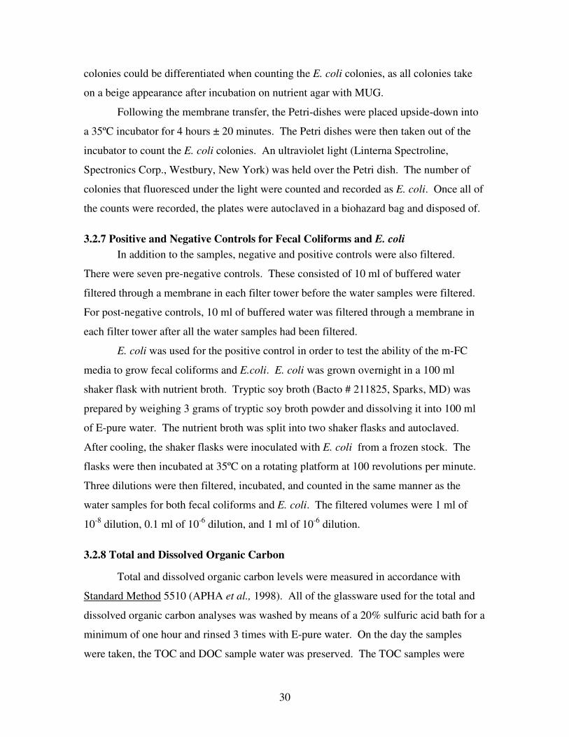
30

colonies could be differentiated when counting the E. coli colonies, as all colonies take on a beige appearance after incubation on nutrient agar with MUG.

Following the membrane transfer, the Petri-dishes were placed upside-down into a 35ºC incubator for 4 hours ± 20 minutes. The Petri dishes were then taken out of the

incubator to count the E. coli colonies. An ultraviolet light (Linterna Spectroline, Spectronics Corp., Westbury, New York) was held over the Petri dish. The number of

colonies that fluoresced under the light were counted and recorded as E. coli. Once all of the counts were recorded, the plates were autoclaved in a biohazard bag and disposed of.

3.2.7 Positive and Negative Controls for Fecal Coliforms and E. coli In addition to the samples, negative and positive controls were also filtered. There were seven pre-negative controls. These consisted of 10 ml of buffered water

filtered through a membrane in each filter tower before the water samples were filtered. For post-negative controls, 10 ml of buffered water was filtered through a membrane in

each filter tower after all the water samples had been filtered. E. coli was used for the positive control in order to test the ability of the m-FC

media to grow fecal coliforms and E.coli. E. coli was grown overnight in a 100 ml shaker flask with nutrient broth. Tryptic soy broth (Bacto # 211825, Sparks, MD) was

prepared by weighing 3 grams of tryptic soy broth powder and dissolving it into 100 ml of E-pure water. The nutrient broth was split into two shaker flasks and autoclaved.

After cooling, the shaker flasks were inoculated with E. coli from a frozen stock. The flasks were then incubated at 35ºC on a rotating platform at 100 revolutions per minute.

Three dilutions were then filtered, incubated, and counted in the same manner as the water samples for both fecal coliforms and E. coli. The filtered volumes were 1 ml of

10-8 dilution, 0.1 ml of 10-6 dilution, and 1 ml of 10-6 dilution.

3.2.8 Total and Dissolved Organic Carbon

Total and dissolved organic carbon levels were measured in accordance with Standard Method 5510 (APHA et al., 1998). All of the glassware used for the total and

dissolved organic carbon analyses was washed by means of a 20% sulfuric acid bath for a minimum of one hour and rinsed 3 times with E-pure water. On the day the samples

were taken, the TOC and DOC sample water was preserved. The TOC samples were

31

poured into 40 ml acid washed glass vials and preserved to a pH of 2 with 40 µl of 6 N HCl. The samples were then stored at 4ºC for a maximum of 2 weeks before analysis.

The DOC samples were filtered through a glass fiber filter (Whatman GF/F filter with 0.7 µm retention). The filters were pre-washed with 20-30 ml of E-pure water. Then, the

sample was passed through the filter. The first 5-10 ml of the sample was discarded and the next 30 ml filtered into a 40 ml acid washed glass vial. The samples were then

preserved to a pH of 2 in the same manner as the TOC samples and stored at 4ºC for up to 2 weeks before analysis.

3.2.8.1 Standard Preparation

The TOC and DOC of the water samples were measured with a Shimadzu TOC-

5000A (Shimadzu Corp., Kyoto, Japan). The TOC and DOC analyzer utilizes a three point calibration curve made with potassium hydrogen phthalate.

First, a stock primary standard of 1000 mg/L was prepared: 0.75 grams of Potassium Hydrogen Phthalate was dried in 103-110ºC oven for 30 minutes and cooled in

a desiccator for an additional 30 minutes. Following the cooling process, 0.5314 grams of the dried Potassium Hydrogen Phthalate was weighed using an analytical balance, and

added to a 250 ml volumetric flask filled half way with E-pure water. The 250 ml flask was then brought up to the mark with E-pure water. The stock primary solution of 1000

mg/L was put in a brown glass bottle and stored at 4ºC for a maximum of 3 weeks. Second, an intermediate standard of 100 mg/L was made. To make the

intermediate standard, 10 ml of the primary stock standard was transferred into a 100 ml volumetric flask half filled with E-pure water. The 100 ml flask was then bought up to

the mark with additional E-pure water. The intermediate standard of 100 mg/L was stored at 4 degrees Celsius for a maximum of 2 days.

The working standards used in the calibration curve were 10, 5, 2, 1, and 0 mg/L. For each working standard, a 100 ml flask was filled half way with E-pure water and 100

µl of 6 N HCl was added to each flask. Then, the appropriate volume of intermediate standard was added to each flask as seen in Table 3. Lastly, the volume in each flask was

brought up to mark with E-pure water.

32

Table 3: Working Standards for TOC/DOC Analysis

Working Standard (mg/L)

Volume of Intermediate Stock Added (ml)

10 10

5 5

2 2

1 1

0 0

3.2.8.2 TOC/DOC Quantification

Once all of the working standard were prepared, the auto-sampler cells for the

Shimadzu TOC-5000A were filled. Each standard and sample was inverted three times, poured into an autosampler vial, and then the vial was covered with parafilm and plastic Shimadzu lids. The standards were placed in the the inner ring of the autosampler rack

from highest to lowest, and then the samples were placed in the outer ring of the autosampler rack. Quality control was established by placing two working standards with

known concentrations in with the sample vials to verify accurate measurements. All standards and samples were sparged for five minutes before analysis to

remove any carbon dioxide and then analyzed three to five times. The standards and samples were measured a minimum of three times, after which the standard deviation and

coefficient of variation were calculated. If the values were not in the desired range (200 for standard deviation and 2.0% for coefficient of variation) after the third measurement,

then another measurement was taken. Measurements were taken until the values were in the desired range or until 5 measurements were taken. Three calibration curves were

produced and the instrument selected the best curve for determining the concentration of each sample.

3.3 Statistical Analysis

Two statistical methods were utilized for analyzing data collected from the

sampling sites: correlation analyses and ANOVA analyses. Correlation analyses were

33

performed on the individual water quality parameters to identify relationships between them. ANOVA analyses were completed to determine differences between different sites

and differences between season with each water quality parameter as well as a complied binary data set for several of the water quality parameters.

3.3.1 Correlation Analysis

Correlation analyses were done using the Microsoft Excel data analysis tool pack.

The data analysis yields an R-value output which is a correlation coefficient representing the linear relationship between the data pairs. Correlation coefficient values range from

-1.00 to +1.00, where the negative sign indicates an inverse correlation. Zero indicates no correlation and 1 indicates complete correlation.

The R-value is used to determine whether a correlation is statistically significant. The two factors that determine whether an R-value shows statistical significance is the

confidence interval used and the number of data pairs that the R-value is generated from. The confidence interval used was a 95% confidence interval, which is commonly used for

research. This is a P-value of 0.05. For example, a statistically siginificant correlation is a P-value of 0.05, and a highly significant correlation would be �0.005. A statistically

significant R-value can be found on a correlation coefficient table with a P-value of 0.05 and the correct number of data points for each parameter.

3.3.2 ANOVA Analysis

The analysis of variance (ANOVA), also known as the F-test, is a method to

determine the variation of the means of a group of data or variables to evaluate statistical significance. ANOVA analyses were done utilizing the Microsoft Excel data analysis

tool pack. The ANOVA test assumes a null hypothesis, which states that there is no difference between the data within a data set. If the analysis is found to be statistically

significant, then the null hypothesis is rejected for the alternative hypothesis. The alternative hypothesis states that the means of the data in the data set are different.

Similar to the correlation analysis, a 95% confidence interval was considered to be statistically significant. A P-value of �0.05 would classify as statistically significant.

The ANOVA analysis was performed with the data segregated by site to determine

34

differences in water quality between the different locations. Then the analysis was repeated with the data organized by season to assess seasonal differences in water quality.

3.3.3 Binary Data Sets

Binary data sets were constructed for further analysis of the data. The binary data

sets were based upon 1 being defined as “polluted” and 0 being defined as “not polluted”. For several of the water quality parameters, a benchmark pollution level was defined.

Any measurement greater than the benchmark pollution level was represented with a 1, and any measurement less than the benchmark pollution level was represented with a

zero. The binary data sets were then analyzed with the ANOVA analysis procedures discussed in the previous section.

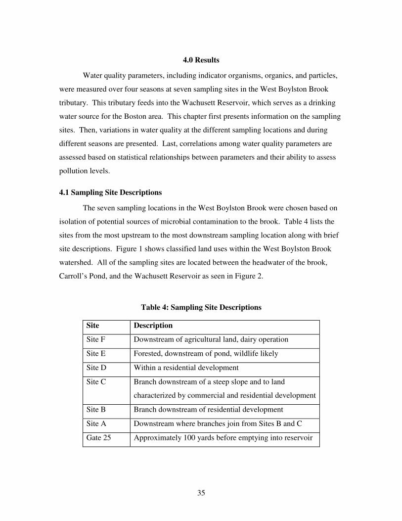
35

4.0 Results

Water quality parameters, including indicator organisms, organics, and particles,

were measured over four seasons at seven sampling sites in the West Boylston Brook tributary. This tributary feeds into the Wachusett Reservoir, which serves as a drinking

water source for the Boston area. This chapter first presents information on the sampling sites. Then, variations in water quality at the different sampling locations and during

different seasons are presented. Last, correlations among water quality parameters are assessed based on statistical relationships between parameters and their ability to assess

pollution levels.

4.1 Sampling Site Descriptions

The seven sampling locations in the West Boylston Brook were chosen based on isolation of potential sources of microbial contamination to the brook. Table 4 lists the

sites from the most upstream to the most downstream sampling location along with brief site descriptions. Figure 1 shows classified land uses within the West Boylston Brook

watershed. All of the sampling sites are located between the headwater of the brook, Carroll’s Pond, and the Wachusett Reservoir as seen in Figure 2.

Table 4: Sampling Site Descriptions

Site Description

Site F Downstream of agricultural land, dairy operation

Site E Forested, downstream of pond, wildlife likely

Site D Within a residential development

Site C Branch downstream of a steep slope and to land characterized by commercial and residential development

Site B Branch downstream of residential development

Site A Downstream where branches join from Sites B and C

Gate 25 Approximately 100 yards before emptying into reservoir

36

����������� ��� ��������������������� ���������������� � ��� ������������� ����������� ��� �����

!�"�#%$ !�&('�)*$ +�&-,-.�/ '0'�1�243 3�576984: ; <�=>=@?

A�B�B B A�B�B C�B�B ���D�E���

FGH

I

JJ�K

LNM O>PRQ S@T UV SNW X Y M Z[ ONM ZNW X\ O>T ] [ O^M Z^W X Z4U�_`ZaX b S>T Uc�d T d T ef`P Z>TRQ S@T UV SNM X d g4d P SaX d O>TRh4Z gaij>P Z g X SaX O^M*h4Z g9i_%SkX Z^M ] l SNW ZDU7h4Z gaic YDb X d ] [ SNm i h4ZNW in>d e@o�pDZ>T�W d X q�h4ZNW ic ZDU d Y m�p4Z>T W i h4Z^WQ O4rEp4Z>T W i h4Z^Wj4S>b X9_`SaX ZNM9_`ZaX b S>T UL4ONmRm>Z^M g4d S>bs T U>Y�W X M d S@bt M l S@Tuf�P Z@Tv M S@T�W4P ONM X SaX d O>T_%S^W X Z7p d W4P ONW S>b_%SkX Z^M_%ODO4U q V ZNM Z>TDT d S@b

Figure 1: Land Uses in the West Boylston Brook Subbasin

37

Figure 2: Sampling Locations in the West Boylston Brook Subbasin Site F is not in the main channel of the West Boylston Brook. Site F is in a

channel that enters the main channel between sites E and D and is located about 50 yards away from Site E. The site is downstream of agricultural land including a small dairy

operation. This site is accessed from Prospect Street and is about 20 yards off the road. As shown in Figure 3, there is board crossing the brook. Samples were collected

immediately upstream of the board. Flow was present at Site F throughout the year.

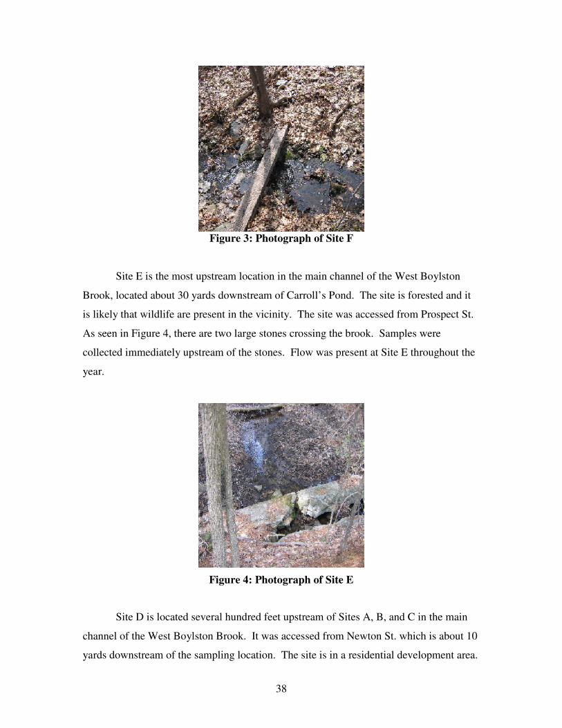
38

Figure 3: Photograph of Site F

Site E is the most upstream location in the main channel of the West Boylston

Brook, located about 30 yards downstream of Carroll’s Pond. The site is forested and it is likely that wildlife are present in the vicinity. The site was accessed from Prospect St.

As seen in Figure 4, there are two large stones crossing the brook. Samples were collected immediately upstream of the stones. Flow was present at Site E throughout the

year.

Figure 4: Photograph of Site E

Site D is located several hundred feet upstream of Sites A, B, and C in the main

channel of the West Boylston Brook. It was accessed from Newton St. which is about 10 yards downstream of the sampling location. The site is in a residential development area.

39

The sampling location is at a large willow tree in the center of a yard as seen in Figure 5. Samples were collected directly in front of the willow tree. Flow was present at Site D

throughout the year except in August 2005 when there was no flow at this location.

Figure 5: Photograph of Site D

Sites A, B, and C were accessed from West Boylston St. directly across from one of the Town of West Boylston’s highway department buildings. Site C is located in a

channel that feeds into the main West Boylston Brook channel downstream of Site B and upstream of Site A. The sampling location is about 50 yards upstream of Site A.

Samples were collected just downstream of a steep slope at a large curvature in the channel as seen in Figure 6. The sampling location is in a wooded area downstream of

commercial and residential development in the Central Street area. Flow was present throughout the year at Site C.

40

Figure 6: Photograph of Site C

Site B is located in the main channel of the West Boylston Brook about 60 yards upstream of Site A. The sampling location is in a wooded area downstream of residential

development. The sampling location is near a large maple tree at a bend in the brook about 20 yards away from West Boylston Street. Samples were collected next to the

maple tree upstream of the bend as seen in Figure 7.

Figure 7: Photograph of Site B

Site A is located where the channel that Site C is located in merges with the main channel of the West Boylston Brook. The sampling site is about 10 feet upstream of a

conduit that carries the brook about 30 yards under West Boylston St. and the adjacent railroad tracks. Samples were collected at the bend in the stream just off the end of a

41

concrete bound laying in the stream bed as seen in Figure 8. Flow was present at Site A throughout the year.

Figure 8: Photograph of Site A

The Gate 25 sampling location is a location that had been used previously by the

DCR for water quality sampling representative of the West Boylston Brook. The site is where the water exits the conduit that carries it under West Boylston St., and is

approximately 100 yards upstream of where the brook enters the Wachusett Reservoir. There is a weir and a stage gage set up at the sampling location and is where stage

readings were obtained for this study. Samples were collected about 1 meter downstream of the weir as seen in Figure 9. There was flow present at Gate 25 throughout the year.

42

Figure 9: Photograph of Sampling Location at Gate 25.

4.2 Sampling Dates Ten sampling events were conducted between February 2005 and February 2006. As shown in Table 5, this included three winter, two spring, three summer and two fall

events. These sampling events were chosen to help understand water quality variability resulting from seasonal differences. Also shown in Table 5 are precipitation conditions

for each sampling event. Dry and wet weather flows were sampled to aid in analyzing contamination levels in the brook. The complete set of water quality parameters was

analyzed for sampling dates from June 2005 to February 2006. Prior to June of 2005, organic carbon measurements and particle counts were not taken.

43

Table 5: Sampling Date with the Season the Sampling Represents

Sampling Date Season

February 23, 2005 Winter

March 30, 2005 Spring

May 24, 2005 * Spring

June 22, 2005 Summer

July 20, 2005 Summer

August 22, 2005 Summer

October 23, 2005 * Fall

November 29, 2005 Fall

January 24, 2006 Winter

February 18, 2006 Winter

* indicates sampling was conducted during a rain event

4.3 Variations in Water Quality Parameters among Sampling Locations

Several water quality parameters showed variations at the different sampling locations on a given sampling date. One of the sampling events that shows many of the

prevalent trends clearly is October 23, 2005. The following sections present water quality at the seven sampling sites for this sampling date. Data from other sampling dates

are also summarized to demonstrate trends in water quality with location in the West Boylston Brook tributary.

4.3.1 Chemical Water Quality Parameters by Site Dissolved oxygen concentrations at the seven sampling sites are shown in Figure

10, along with the temperature. The dissolved oxygen concentration tended to increase

towards the more downstream locations. Dissolved oxygen levels on October 23, 2005 ranged from a low of 9.9 mg/L at Site E to a high of 11.2 mg/L at Gate 25. The dissolved

oxygen at Gate 25 was 13% higher than at Site E. The temperature ranged from 9.0°C at Sites D and E to 9.8°C at Site C.

44

8.6

8.8

9.0

9.2

9.4

9.6

9.8

10.0

Gate 25Site ASite BSite CSite DSite ESite F

Sampling Site

Tem

pera

ture

(deg

rees

Cel

sius)

9.0

9.5

10.0

10.5

11.0

11.5

Diss

olve

d O

xyge

n (m

g/L)

Temperature Dissolved Oxygen

Figure 10: Temperatures and Dissolved Oxygen Levels on October, 23 2005

The high temperature at Site C is most likely due to groundwater influences on the brook. Seasonally, the temperature at Site C is higher in the winter compared to the

other six sites, and lower in the summer than at any of the other sampling locations. The characteristics of the stream-flow in the brook have a direct affect on the re-

aeration rate of the water which in turn affects the amount of dissolved oxygen that will be present. Table 6 lists the ranges of dissolved oxygen observed over the course of the

entire sampling period along with a listing of the sites with the highest and lowest dissolved oxygen levels. Sites C and E tended to have low dissolved oxygen levels in

comparison to other sampling locations. Gate 25, Site B, and Site F tended to have high dissolved oxygen levels in comparison to the other sampling locations.

45

Table 6: Dissolved Oxygen Ranges Sampling Date

DO Range (mg/L)

Site of Lowest DO Site of Highest DO

Feb. 05 (Winter) 10.6 - 12.9 Site C Gate 25

Mar. 05 (Spring) 11.2 - 12.6 Site C Gate 25

May 05 (Spring) 10.5 - 11.8 Site E Site B

Jun. 05 (Summer) 8.3 - 10.3 Site C Site F

Jul. 05 (Summer) 5.9 - 8.0 Site E Site B

Aug. 05 (Summer) 7.3 - 9.6 Site C Site F

Oct. 05 (Fall) 9.9 - 11.2 Site E Gate 25

Nov. 05 (Fall) 7.4 - 10.1 Site C Gate 25

Jan. 06 (Winter) 9.7 - 13.4 Site C Gate 25

Feb. 06 (Winter) 10.3 - 14.0 Site C Gate 25

The flow characteristics at Gate 25, Site B, and Site F may have contributed to the

elevated levels of dissolved oxygen measured at these locations. The dissolved oxygen content of the water at Gate 25 is measured just downstream of a sharp crested, v-notch

weir which causes significant mixing and re-aeration. The flow at sites B and F is fast moving compared to the other sites due to a steeper slope at these locations. Also, the

channel bottom at sites B and F is rocky, which contributes to mixing and thus reaeration at these sites.

Site E tended to have the lowest levels of dissolved oxygen which is probably due to the nature of the flow at that site. The water is very slow moving with a smooth silt

covered channel bottom due to some ponding in the stream. There appears to be little reaeration of the water at Site E. Site C may have low levels of dissolved oxygen due to

a low flow at this location or due to groundwater influences on the brook. Conductivity and pH levels at the seven sampling sites on October 23, 2005 are

shown in Figure 11. The pH and conductivity appear to follow similar trends for most sites. The conductivity in the brook ranged from 110 µS at Site C to 203 µS at Site F, a

46% difference. There was a modest increase in conductivity from Site C downstream to

46

Site Gate 25; however no apparent trend at the upstream sites. The pH ranged from 6.71 at Site C to 7.39 at Gate 25.

6.20

6.40

6.60

6.80

7.00

7.20

7.40

7.60

Gate 25Site ASite BSite CSite DSite ESite F

Sampling Site

pH

0

50

100

150

200

250

Con

duct

ivity

(mS)

pHConductivity

Figure 11: pH and Conductivity on October 23, 2005

Table 7 lists the range of conductivity measured during each sampling event,

along with the sites which had the highest and lowest values. Site E tended to have low conductivity levels in comparison to the other sample locations. High conductivity levels

were sporadically found at several of the other sampling locations. The high conductivities were expected in downstream sites around more developed areas.

Inorganic suspended solids from runoff as well as the presence of chloride and nitrate from failing septic systems will increase conductivity levels.

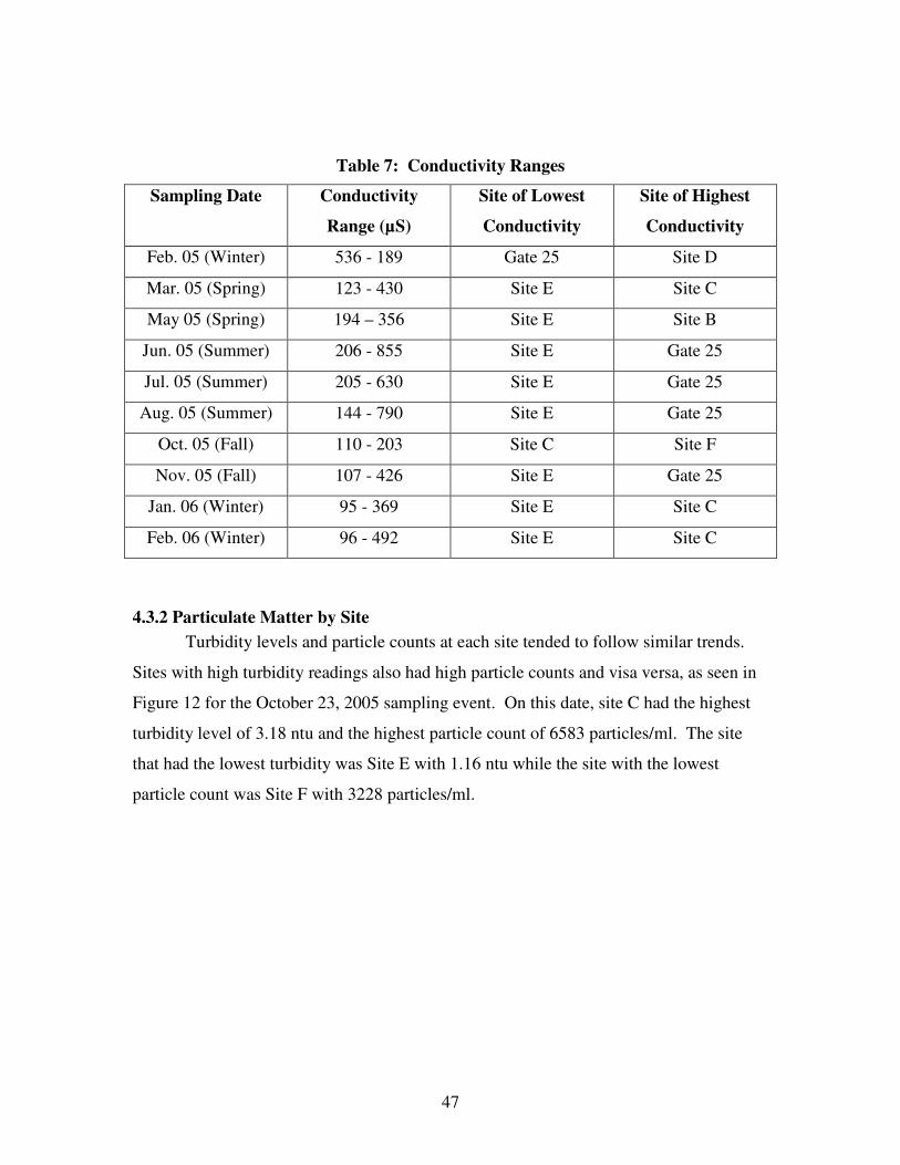
47

Table 7: Conductivity Ranges Sampling Date

Conductivity Range (µS)

Site of Lowest Conductivity

Site of Highest Conductivity

Feb. 05 (Winter) 536 - 189 Gate 25 Site D

Mar. 05 (Spring) 123 - 430 Site E Site C

May 05 (Spring) 194 – 356 Site E Site B

Jun. 05 (Summer) 206 - 855 Site E Gate 25

Jul. 05 (Summer) 205 - 630 Site E Gate 25

Aug. 05 (Summer) 144 - 790 Site E Gate 25

Oct. 05 (Fall) 110 - 203 Site C Site F

Nov. 05 (Fall) 107 - 426 Site E Gate 25

Jan. 06 (Winter) 95 - 369 Site E Site C

Feb. 06 (Winter) 96 - 492 Site E Site C

4.3.2 Particulate Matter by Site Turbidity levels and particle counts at each site tended to follow similar trends.

Sites with high turbidity readings also had high particle counts and visa versa, as seen in Figure 12 for the October 23, 2005 sampling event. On this date, site C had the highest

turbidity level of 3.18 ntu and the highest particle count of 6583 particles/ml. The site that had the lowest turbidity was Site E with 1.16 ntu while the site with the lowest

particle count was Site F with 3228 particles/ml.

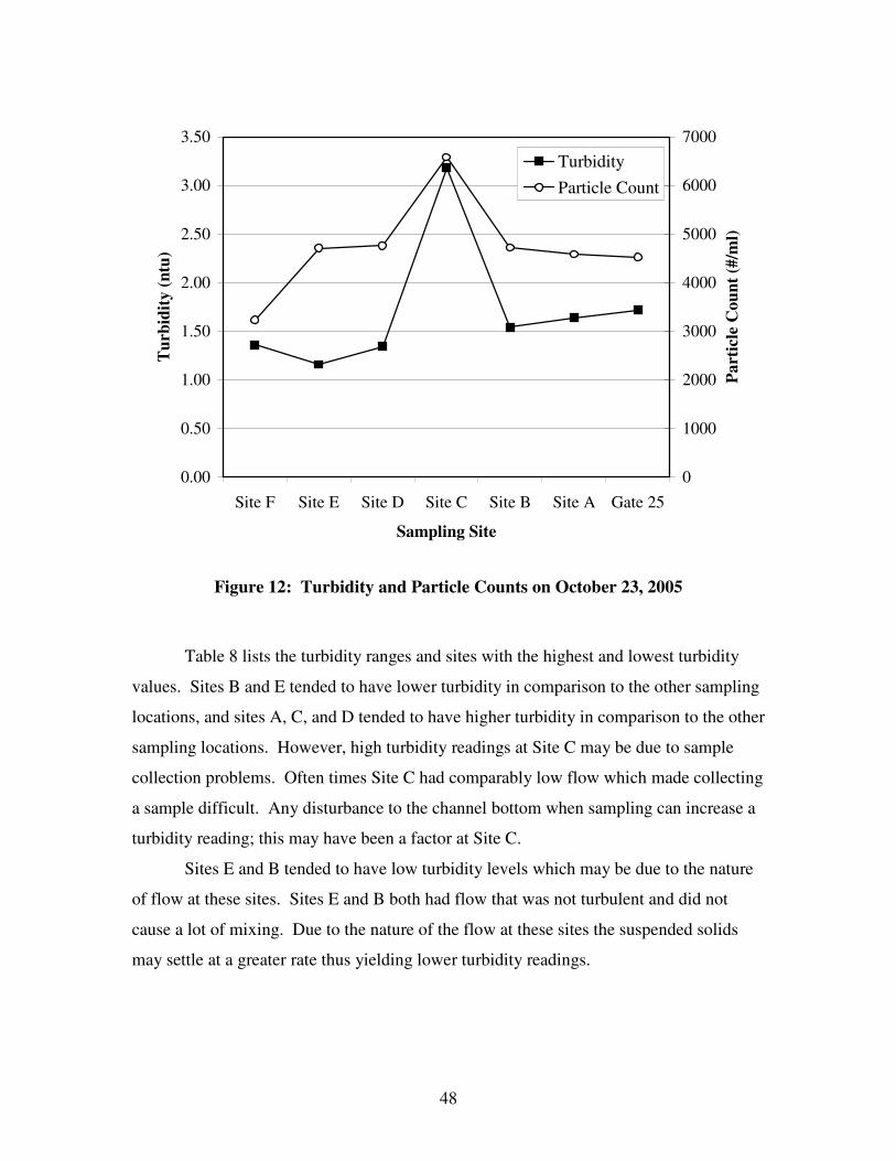
48

0.00

0.50

1.00

1.50

2.00

2.50

3.00

3.50

Gate 25Site ASite BSite CSite DSite ESite F

Sampling Site

Turb

idity

(ntu

)

0

1000

2000

3000

4000

5000

6000

7000

Part

icle

Cou

nt (#

/ml)

TurbidityParticle Count

Figure 12: Turbidity and Particle Counts on October 23, 2005

Table 8 lists the turbidity ranges and sites with the highest and lowest turbidity

values. Sites B and E tended to have lower turbidity in comparison to the other sampling locations, and sites A, C, and D tended to have higher turbidity in comparison to the other

sampling locations. However, high turbidity readings at Site C may be due to sample collection problems. Often times Site C had comparably low flow which made collecting

a sample difficult. Any disturbance to the channel bottom when sampling can increase a turbidity reading; this may have been a factor at Site C.

Sites E and B tended to have low turbidity levels which may be due to the nature of flow at these sites. Sites E and B both had flow that was not turbulent and did not

cause a lot of mixing. Due to the nature of the flow at these sites the suspended solids may settle at a greater rate thus yielding lower turbidity readings.

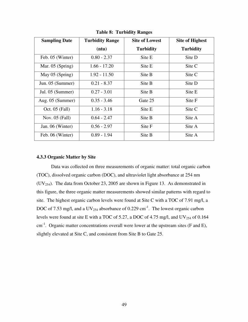
49

Table 8: Turbidity Ranges Sampling Date

Turbidity Range

(ntu) Site of Lowest

Turbidity Site of Highest

Turbidity

Feb. 05 (Winter) 0.80 - 2.37 Site E Site D

Mar. 05 (Spring) 1.66 - 17.20 Site E Site C

May 05 (Spring) 1.92 - 11.50 Site B Site C

Jun. 05 (Summer) 0.21 - 8.37 Site B Site D

Jul. 05 (Summer) 0.27 - 3.01 Site B Site E

Aug. 05 (Summer) 0.35 - 3.46 Gate 25 Site F

Oct. 05 (Fall) 1.16 - 3.18 Site E Site C

Nov. 05 (Fall) 0.64 - 2.47 Site B Site A

Jan. 06 (Winter) 0.56 - 2.97 Site F Site A

Feb. 06 (Winter) 0.89 - 1.94 Site B Site A

4.3.3 Organic Matter by Site

Data was collected on three measurements of organic matter: total organic carbon (TOC), dissolved organic carbon (DOC), and ultraviolet light absorbance at 254 nm

(UV254). The data from October 23, 2005 are shown in Figure 13. As demonstrated in this figure, the three organic matter measurements showed similar patterns with regard to

site. The highest organic carbon levels were found at Site C with a TOC of 7.91 mg/l, a DOC of 7.53 mg/l, and a UV254 absorbance of 0.229 cm-1. The lowest organic carbon

levels were found at site E with a TOC of 5.27, a DOC of 4.75 mg/l, and UV254 of 0.164 cm-1. Organic matter concentrations overall were lower at the upstream sites (F and E),

slightly elevated at Site C, and consistent from Site B to Gate 25.

50

0.00

1.00

2.00

3.00

4.00

5.00

6.00

7.00

8.00

9.00

Gate 25Site ASite BSite CSite DSite ESite F

Sampling Site

Org

anic

Car

bon

(mg/

L)

0.000

0.050

0.100

0.150

0.200

0.250

Abs

orba

nce

(1/c

m)

Total OrganicCarbonDissolved OrganicCarbonUV Absorbance

Figure 13: Organic Carbon and UV254 Absorbance Levels on October 23, 2005

Table 9 lists the range of TOC observed on each of the sampling dates and where levels where highest and lowest. Unlike October 2005, Site C tended to have the lowest

levels of TOC during the other summer, fall, and winter sampling events. Site E had the highest levels of TOC on four of the seven sampling events. This was not unexpected as

Site E is located just downstream of a wooded wetland.

51

Table 9: Total Organic Carbon Ranges Sampling Date

Total Organic Carbon Range

(mg/L)

Site of Lowest Total Organic

Carbon

Site of Highest Total Organic

Carbon

Feb. 05 (Winter) Not Measured

Mar. 05 (Spring) Not Measured

May 05 (Spring) Not Measured

Jun. 05 (Summer) 1.04 - 3.97 Site C Site E

Jul. 05 (Summer) 1.26 - 5.49 Site C Site E

Aug. 05 (Summer) 1.32 - 4.06 Gate 25 Site E

Oct. 05 (Fall) 5.27 - 7.91 Site E Site C

Nov. 05 (Fall) 5.09 - 7.92 Site C Site D

Jan. 06 (Winter) 2.77 - 3.42 Site C Site D

Feb. 06 (Winter) 2.04 - 3.07 Site C Site E

4.3.4 Indicator Organisms by Site

Two biological indicator organisms, fecal coliforms and E. coli, were measured to

assess possible locations where microbial contamination was entering the West Boylston Brook. Concentrations of the indicators for the October 23, 2005 sampling date are

shown in Figure 14. In general, the two indicators tended to vary by site in a similar fashion. This is to be expected as E. coli are a subset of the fecal coliform bacteria group.

On October 23, 2005, the fecal coliforms ranged from 42 cfu/100 ml at Site E to 1322 cfu/100 ml at Gate 25. E. coli levels ranged from 42 cfu/100 ml at Site E to 861 cfu/100

ml at Gate 25.

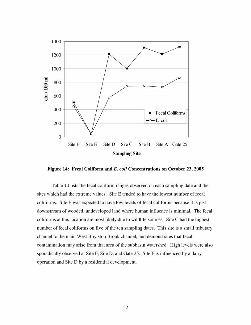
52

0

200

400

600

800

1000

1200

1400

Gate 25Site ASite BSite CSite DSite ESite F

Sampling Site

cfu

/ 100

ml

Fecal ColiformsE. coli

Figure 14: Fecal Coliform and E. coli Concentrations on October 23, 2005

Table 10 lists the fecal coliform ranges observed on each sampling date and the

sites which had the extreme values. Site E tended to have the lowest number of fecal coliforms. Site E was expected to have low levels of fecal coliforms because it is just

downstream of wooded, undeveloped land where human influence is minimal. The fecal coliforms at this location are most likely due to wildlife sources. Site C had the highest

number of fecal coliforms on five of the ten sampling dates. This site is a small tributary channel to the main West Boylston Brook channel, and demonstrates that fecal

contamination may arise from that area of the subbasin watershed. High levels were also sporadically observed at Site F, Site D, and Gate 25. Site F is influenced by a dairy

operation and Site D by a residential development.

53

Table 10: Fecal Coliform Ranges Sampling Date

Fecal Coliform Range (cfu/100ml)

Site with Lowest Number of Fecal

Coliforms

Site with Highest Number of Fecal

Coliforms

Feb. 05 (Winter) 7 - 64 Site C Site D

Mar. 05 (Spring) 14 - 410 Site E Site C

May 05 (Spring) 450 - 4800 Site E Site C

Jun. 05 (Summer) 35 - 387 Site E Gate 25

Jul. 05 (Summer) 85 - 377 Site E Site F

Aug. 05 (Summer) 280 - 1109 Gate 25 Site C

Oct. 05 (Fall) 42 - 1322 Site E Gate 25

Nov. 05 (Fall) 97 - 2667 Site E Site F

Jan. 06 (Winter) 141 - 487 Sites E and F Site C

Feb. 06 (Winter) 8 - 787 Site E Site C

4.4 Variation in Water Quality Parameters by Season

The water quality parameters discussed in Section 4.3 were also analyzed by

season to determine impacts of seasonal changes on pollutant levels. Some of the water quality parameters show strong seasonal trends while other water quality parameters do

not vary significantly during the year. The water quality measurements from Gate 25, which are presented in the following sections, show a representation of the entire sub-

watershed basin and how the seasonal changes affect the water quality of the basin.

4.4.1 Chemical Water Quality Parameters by Season

Temperature and dissolved oxygen followed clear seasonal trends, as seen in Figure 15. Temperature was greater in the summer months than the winter months. The

temperature at Gate 25 ranged from 2.2°C in February of 2006 to 15.0°C in July and August of 2005. The other sites followed the same seasonal patterns.

The dissolved oxygen concentration was inversely related to the temperature. This was expected as saturation values of dissolved oxygen decrease with increasing

54

temperature. Dissolved oxygen at Gate 25 ranged from 8.1 mg/l in July of 2005 to 14.0 mg/L in February of 2006. There were similar seasonal temperature and dissolved

oxygen trends at the other six sampling locations.

0

2

4

6

8

10

12

14

16

February

05

March 05

May 05

June 05

July 05

August

05

October

05

Novem

ber 05

Januar

y 06

February

06

Sampling Event

Tem

pera

ture

(deg

rees

C)

0.0

2.0

4.0

6.0

8.0

10.0

12.0

14.0

16.0

Diss

olve

d O

xyge

n (m

g/L)

T emperatureDissolved Oxygen

Figure 15: Temperature and Dissolved Oxygen Concentration at Gate 25

The conductivity and pH measured at Gate 25 over the four seasons is shown in

Figure 16. The pH was reasonably consistent throughout the sampling period. The lowest pH of 6.8 occurred in May of 2005 and the highest pH of 7.5 occurred in February

of 2006. There were no clear seasonal trends at any of the seven sampling locations. Also shown in Figure 16 is the conductivity at Gate 25. Conductivity ranged

from 170 µS in October of 2005 to 855 µS in June of 2005. At Gate 25, the conductivity was higher in the summer months than the rest of the year. The highest summer

conductivity was 855 µS in June of 2005, while the highest winter conductivity was 536 µS in February of 2005. In the spring, conductivity was highest in March 2005 at 372

µS, and in the fall was 426 µS in November 2005. All of the other sampling locations had similarly high conductivities in the summer months except Site C. Site C did not seem to show any seasonal trends. The conductivity stayed relatively constant

throughout the year with an average of 417 µS, but peaked in February of 2005 to a level of 803 µS.

55

01

23

45

67

8

February

05

March 05

May 05

June 05

July 05

August

05

October

05

Novem

ber 05

Januar

y 06

February

06

Sampling Event

pH

0100200300400500600700800900

Con

duct

ivity

(uS)

pHConductivity

Figure 16: Conductivity and pH at Gate 25

4.4.2 Particulate Matter by Season

The turbidity and particle count data from Gate 25 are shown in Figure 17. Particle count data was available from June 2005 onward. Seasonal trends are not readily

apparent at Gate 25 nor any of the other sampling locations. Over the 13-month sampling period, the turbidity ranged from 0.35 ntu in August of 2005 to 3.38 ntu in March of

2005. The lowest particle count at Gate 25 was 1032 particles/ml in August of 2005 and the highest particle count was 4524 particles/ml in October of 2005.

Although the turbidity and particle count data did not show seasonal trends, these two parameters where thought to be dependent upon climate or more specifically

precipitation conditions and flow conditions. Sampling in May 2005 and October 2005 was conducted during rainfall events. There was higher turbidity at Gate 25 in May 2005

and October 2005 in comparison to other sampling events, but the trend was not as apparent as expected. Other sites were similar with regard to particulate matter, in that a

trend between rainfall data and the two particle measurements was not apparent.

56

0.000.50

1.001.502.00

2.503.00

3.504.00

February

05

March 05

May 05

June 05

July 05

August

05

October

05

Novem

ber 05

Januar

y 06

February

06

Sampling Event

Turb

idity

(ntu

)

0500100015002000250030003500400045005000

Part

icle

s (#/

ml)

T urbidity

Particles

Figure 17: Turbidity and Particle Counts at Gate 25

4.4.3 Organic Matter by Season

Organic carbon data were measured from June of 2005 through February of 2006.

As shown in Figure 18, organic carbon levels were higher in the fall than in the winter and summer months. The highest TOC concentration was observed in November of 2005

at 6.62 mg/l. In the summer, TOC values ranged from 1.28 mg/l to 2.87 mg/l, while in the winter levels ranged from 2.31 mg/l to 3.34 mg/l. The TOC on January 24, 2006 is

about 50 percent lower than the total organic carbon on November 29, 2005. The DOC and UV254 levels at Gate 25 followed the same seasonal trends as the

TOC. The highest DOC concentration was 6.42 mg/l in October of 2005 and the lowest DOC concentration was 1.28 mg/L in June of 2005. The highest UV254 absorbance was

0.215 cm-1 in October of 2005, and the lowest UV254 absorbance 0.043 cm-1 in June of 2005. High organic carbon measurements in the fall months are most likely due to falling

leaves entering the water, thus adding organic matter to the water. All of the sampling locations had similar seasonal organic carbon trends except

for Site E. At Site E, the TOC and DOC followed the same seasonal trends as the other sampling locations, but the UV254 did not. UV254 levels did not reveal any seasonal trend

and were relatively high in the spring months when the TOC and DOC were

57

comparatively low. The UV254 at Site E ranged from 0.069 cm-1 in February of 2006 to 0.183 cm-1 in July of 2005.

0.000

1.000

2.000

3.000

4.000

5.000

6.000

7.000

June 0

5

July 0

5

August

05

October

05

Novem

ber 05

Januar

y 06

Februar

y 06

Sampling Event

Org

anic

Car

bon

(mg/

L)

0

0.05

0.1

0.15

0.2

0.25

UV

Abs

orba

nce

(1/c

m)

TOC

DOC

UV

Figure 18: Organic Carbon Levels and UV254 Absorbance at Gate 25

4.4.4 Indicator Organisms by Season

Figure 17 presents the fecal coliform and E. coli concentrations at Gate 25 for the

ten sampling events. The fecal coliforms range from 35 cfu/100 ml in March of 2005 to 1322 cfu/100 ml in October of 2005. The only apparent seasonal trend is that the fecal

coliform levels are lower in the winter months. Lower levels were expected during the winter because cold temperatures cause microorganisms to die off at a faster rate. E. coli

concentrations at Gate 25 range from 35 cfu/100 ml in March of 2005 to 861 cfu/100 ml in October of 2005.

Each of the other sampling locations had similar seasonal trends as Gate 25 excluding Site C. Fecal coliform and E. coli levels were much lower in the winter

months, and there were spikes in indicator organism levels during various months outside of the winter season. All of the sampling sites except sites E and F had high levels in

May and October which is most likely due to rain events during both of these sampling events.

58

0

200

400

600

800

1000

1200

1400

February

05

March 05

May 05

June 05

July 05

August

05

October

05

Novem

ber 05

Januar

y 06

February

06

Sampling Event

cfu

/ 100

ml

Fecal Coliforms

E. coli

Figure 19: Fecal Coliform and E. coli levels at Gate 25

Site C yielded some interesting indicator organism data. The fecal coliform and E. coli concentrations at Site C were not lower in the winter months than the other

seasons, as seen in Figure 20. The fecal coliforms at Site C ranged from 7 to 787 cfu/100 ml in the winter, from 410 to 4800 cfu/100 ml in the spring, from 191 to 1109 cfu/100 ml

in the summer, and from 121 to 1000 cfu/100 ml in the fall. There was not a dramatic drop in indicator organisms at Site C during the winter months.

59

0

1000

2000

3000

4000

5000

6000

February

05

March 05

May 05

June 05

July 05

August

05

October

05

Novem

ber 05

Januar

y 06

February

06

Sampling Event

cfu

/ 100

ml

Fecal Coliforms

E. coli

Figure 20: Fecal Coliform and E. coli Levels at Site C

4.5 Statistical Analysis

Several statistical analyses were performed on the water quality data collected throughout this study. The following sections present the data analyses, which were

conducted using Microsoft Excel data analysis tools. First, a correlation analysis was performed to identify relationships between the water quality parameters. Second, ANOVA analysis was completed to determine differences between water quality at

different sites and differences between seasons. Lastly, the water quality data were converted to a binary data set and analyzed with an ANOVA analysis to determine the

relative capacity of water quality parameters to characterize the tributary as polluted or unpolluted.

4.5.1 Correlation Analysis

A correlation analysis was used to determine relationships between water quality

parameters. The correlation analysis performed by Microsoft Excel provides an R-value as an output for each pair of water quality parameters. An R-value shows how well two

water quality parameters are correlated with one-another. An R-value of 1 shows complete correlation, and an R-value of 0 shows no correlation. A negative R-value

60

indicates an inverse correlation, and similarly an R-value of -1 shows complete inverse correlation.

The correlation analysis was based on a 95% confidence level, or a P-value of 0.05. In order to determine if a statistically significant correlation exists, a minimum R-

value must be determined from a correlation coefficient table. Minimum R-values are based upon the number of data points, n, which are evaluated. The number of data points

in this study ranged from 41 data points (UV254) to 65 data points (majority of the other parameters) and are summarized in Table 11. As shown in this table, for example, an R-

value of 0.312 shows a statistically significant correlation between any of the other water quality parameters and UV254.

Table 12 provides the Excel output for the correlation analysis of the water quality data collected in this study. Comparison of the R-values in this table to minimum

values in Table 11 reveals which parameters have statistically significant correlations. The correlations are highlighted n bold in Table 12.

Table 11: Number Data Points for each Water Quality Parameter and the Minimum R-Values Needed Statistically Significant Correlation (95% Confidence

Level) Water Quality Parameter Number of Data Points (n) Minimum R-Value

Temperature 65 0.279 Dissolved Oxygen 65 0.279 Conductivity 65 0.279 pH 65 0.279 UV254 41 0.312 TOC 48 0.294 DOC 48 0.294 Turbidity 65 0.279 Particles 48 0.294 FC 65 0.279 E. coli 65 0.279

61

Table 12: R-Values for Correlation Analysis on Water Quality Data

Temp. DO Cond. pH UV TOC DOC Turbid. Partic. FC E. coli Temp 1 DO -0.763 1 Cond. 0.282 -0.163 1 pH -0.157 0.242 -0.097 1 UV 0.077 0.107 -0.607 -0.005 1 TOC -0.254 0.095 -0.619 0.004 0.728 1 DOC -0.087 0.004 -0.575 -0.071 0.835 0.965 1 Turbidity 0.093 0.057 0.004 -0.123 0.187 0.048 0.075 1 Particles -0.195 0.307 -0.492 0.265 0.654 0.516 0.521 0.532 1 FC 0.071 -0.065 -0.160 -0.230 0.357 0.468 0.469 0.360 0.145 1 E. coli -0.020 -0.008 -0.160 -0.196 0.263 0.525 0.470 0.397 0.168 0.965 1

Overall there were 21 pairs of water quality parameters that were statistically

correlated to one another (16 directly correlated and 5 inversely correlated) out of a possible 55 pairings. Table 13 lists all of the correlated pairs. pH was the only water

quality parameter that did not show any correlation to any of the other water quality parameters. Conductivity and dissolved oxygen were both correlated with temperature.

Dissolved oxygen showed an expected inverse correlation to temperature. As temperature increases the saturation level of dissolved oxygen in water decreases which

yields an inverse correlation between the two parameters. The correlation between temperature and conductivity may be due to biological

processes. Biological processes that affect conductivity (i.e. the degradation of organic matter) are affected by temperature and therefore may be the source of the correlation

between temperature and conductivity. Conductivity was also inversely related to organic matter which was to be expected because organic matter does not carry a charge.

Conductivity was also inversely correlated with particle counts. This inverse correlation shows that the majority of the particulate matter in the water was organic which supports

the correlation between conductivity and temperature. Particle counts were also correlated to all of the organic carbon measurements, again showing that the particulate

matter in the water was for the most part organic matter. Turbidity was not correlated to any organic matter measurements even though

turbidity was correlated with particle counts. The turbidity is not a measure of the

62

organic matter, but instead a measure of small inorganic dissolved particles. It is important to note that although turbidity and particle counts correlate to one another, they

are representative of different types of particles. Each of the organic carbon measurements and particulate matter measurements

were correlated to each indicator microorganism with the exception that UV254 did not correlate with E. coli. These correlations are most likely because microorganisms can

attach to solids found in water which increases their survival rates.

Table 13: Correlations between Water Quality Parameters

Direct Correlation Inverse Correlation

Temperature + Conductivity UV254 + TOC UV254 + DOC

UV254 + Particle Counts UV254 + Fecal Coliforms

TOC + DOC TOC + Particle Counts

TOC + Fecal Coliforms TOC + E. coli

DOC + Particle Counts DOC + Fecal Coliforms

DOC + E. coli

Turbidity + Particle Counts

Turbidity + Fecal Coliforms Turbidity + E. coli

Fecal Coliforms + E. coli

Temperature + Dissolved Oxygen Conductivity + UV254 Conductivity + TOC

Conductivity + DOC Conductivity + Particle Counts

63

4.5.1.1 Correlation Analysis with Stage Height

Further correlation analysis was carried out in the same manner as in the previous

section to determine if any of the water quality parameters were correlated with stage height. There were 10 data points of stage height (1 for each sampling event), but 7

measurements at the 7 sites. An R-value of 0.632 or greater indicated a correlation. Stage height was found to be directly correlated with particles and organic carbon (TOC,

DOC, and UV254), and inversely correlated with conductivity. The R-values for each of the water quality parameters that had a correlation with stage height are listed in Table

14.

Table 14: R-Values for each Water Quality Parameter Correlated with Stage Height Water Quality Parameter R-value

UV254 0.965

DOC 0.771

Particles 0.766

Conductivity -0.762

TOC 0.711

4.5.2 ANOVA Analysis

ANOVA analysis was performed to determine the differences between sites and the differences between the seasons for each of the water quality parameters. For site

analysis, the null hypothesis was that the mean of the data for each constituent in the sub-basin was the same at every site. For the seasonal analysis, the null hypothesis was that

the mean of the data for each constituent was the same for every season. The ANOVA analysis was based upon a 95% confidence level or a P-value of 0.05. Thus, for a P-value

of less than or equal to 0.05, the null hypothesis was rejected.

4.5.2.1 ANOVA Site Analysis

Differences in the eleven water quality parameters were analyzed according to site variations between the seven sampling sites. There were a different number of data

64

points at each site and for each water quality parameter. The specific numbers of data points are shown in Table 15. TOC, DOC, UV254 and particle counts have fewer data

points because they were not measured until the June 2005 sampling event. Site D also has fewer data points because low or no flow prevented sampling on August 2005.

Table 15: Number of Data Points for the ANOVA Site Analyses Sites Parameter

Gate 25

Site A

Site B

Site C

Site D

Site E

Site F

Temperature, DO, Conductivity, pH, Turbidity, Fecal Coliforms, E. coli

10 9 9 10 9 10 7

TOC, DOC, Particle Counts

7 7 7 7 6 7 7

UV254

6 6 6 6 5 6 6

The ANOVA analyses by site are presented in Appendix B, and Table 16 lists the P-values for each of the water quality parameters according to variation by site. The two

water quality parameters that were found to be statistically different by site (P-value �0.05) are conductivity and pH. All of the other water quality parameters were not

statistically different by site. The different surrounding materials and land uses at each site most likely factor into the variation in the two water quality parameters by sampling

location. Gate 25 had the highest conductivity levels with an average of 481 µS, and Site E had the lowest with an average of 139 µS. Site D had the highest pH levels with an

average of 7.3 and Site C had the lowest with an average of 6.8. One water quality parameter that was expected to be statistically different by site

was dissolved oxygen. The flow characteristics at each site were expected to cause site variations in dissolved oxygen levels, but this result was not found.

Fecal coliforms and E. coli were found to not be statistically different by site. This result ruled out any one site being specified as a source of biological contamination.

The biological contamination seems to be spread throughout the entire watershed subbasin.

65

Table 16: P-Values for Each Water Quality Parameter According to Variations by Site

Water Quality Parameter P-Value

Conductivity 3.37×10-5

pH 1.26×10-3

Dissolved Oxygen 0.125

Particle Count 0.146

Turbidity 0.179

UV254 0.332

Fecal Coliforms 0.301

E. coli 0.447

DOC 0.686

TOC 0.693

Temperature 0.987

4.5.2.2 ANOVA Seasonal Analysis

Differences in the eleven water quality parameters were analyzed to determine seasonal variations. There are a different number of data points for each of the water

quality parameters and each of the seasons, as shown in Table 17. The data points are totaled from the 3 winter, 2 spring, 3 summer and 2 fall sampling events. The ANOVA

analysis for TOC, DOC, UV254 and particle counts is based on only 3 seasons.

Table 17: Number of Data Points for the ANOVA Seasonal Analyses Season Parameter

Winter Spring Summer Fall

Temperature, DO, Conductivity, pH, Turbidity, Fecal Coliforms, E. coli

18 12 20 14

TOC, DOC, Particle Counts

14 0 20 14

UV254

14 0 19 14

66

The ANOVA results for the seasonal analyses are presented in Appendix C and summarized in Table 18 which lists the P-values for each of the water quality parameters

according to variation by season. All of the water quality parameters were found to be statistically different by season. Several water quality parameters were expected to be

statistically different by season. Due to seasonal temperature changes in New England, it was expected that temperature would be statistically different by season as well as

dissolved oxygen which is inversely correlated to temperature based on saturation values of dissolved oxygen at different temperatures.

Table 18: P-Values for Each Water Quality Parameter According to Variation by Season

Water Quality Parameter P-Value

Temperature 4.15×10-24

TOC 2.80×10-16

DOC 3.67×10-15

Dissolved Oxygen 1.84×10-12

pH 7.16×10-4

UV254 2.00×10-4

Conductivity 1.89×10-3

Turbidity 7.11×10-3

Particle Count 0.016

E. coli 0.018

Fecal Coliforms 0.023

It was also expected that fecal coliform levels and E. coli levels would be statistically different by season. Temperature affects the survival of these

microorganisms; thus concentrations tend to be higher in warmer verses colder temperatures due to increased survival times. Fecal coliform levels averaged 165 cfu/100

ml in the winter months verses an average of 301 cfu/100 ml in the summer months. A seasonal trend in microorganisms that was not expected was the high average levels in

the spring and fall which were 684 cfu/100 ml and 847 cfu/100 ml, respectively.

67

Organic matter measurements (TOC, DOC and UV254) all differed by season as well. It was expected that organic matter may differ by season due to additional organic

matter entering the water in the fall season from the large amount of leaves that fall into the brook. This theory seemed accurate as the fall sampling events had the highest

average TOC value of 6.6 mg/l, verses an average of 3.2 mg/l in the winter and an average of 2.4 mg/l in the summer.

Turbidity and particle counts varied by season as well. It was expected that they may vary by season due to high flows in the spring causing erosion, thus increasing

turbidity and particle counts. It was also expected that leaves entering the brook in the fall may increase turbidity and particle counts. Turbidity was high in the spring, but not

in the fall. The average turbidity in the spring was 4.5 ntu, while the next highest average turbidity was 2.1 ntu in the summer months. Particle counts were highest in the fall with

an average count of 3725 /ml. Average counts in the winter and summer were 3535/ml and 2301/ml, respectively.

pH and conductivity differed by season as well. The variation by season shows the difference in material entering the brook throughout the year, which could be caused

by a number of factors. One example would be a large amount of organic matter entering the brook in the fall causing lower conductivity measurements.

4.5.3 ANOVA Analysis of the Binary Data Set

Binary data sets were created for several of the water quality parameters for the

purpose of further ANOVA analysis to assess pollution levels in the brook. The binary data set was created by setting a bench mark level for several of the water quality

parameters. Any data point in the data set that was greater than the specified bench mark level was considered to be “polluted” and any value less than the specified bench mark

levels was considered to be “not polluted”. Binary data sets were created for the following parameters: conductivity,

turbidity, fecal coliforms, E. coli, and SUVA. Benchmark levels are shown in Table 19. Water quality parameters such as temperature, pH, and dissolved oxygen were not

included in the binary data sets due to the lack of good benchmark levels for these

68

parameters. In this research, the temperature, pH and dissolved oxygen were all in ranges normal for surface waters and would therefore not be classified as “polluted”.

The conductivity benchmarks of 150 and 500 µS are based upon the EPA’s definition of a healthy freshwater fishery (EPA, 2005e). The turbidity benchmark of 5

ntu is based upon the turbidity requirement to avoid filtration of a surface water source for a public water supply (EPA, 1991). The SUVA benchmark is based upon the EPA’s

required level of organic carbon removal to reduce disinfection byproducts in drinking water treatment plants. SUVA can be calculated using Equation 1 (EPA, 2006b). The

fecal coliform and E. coli levels are based upon the EPA’s guidelines for safe body contact with a water (EPA, 2006a).

( )( ) 100*

/

1254

LmgDOCcmUV

SUVA−

= (Equation 1)

Table 19: Benchmark Pollution Levels Water Quality Parameter Benchmark Levels Source

Conductivity > 150 µS < 500 µS EPA “freshwater fishery”

Turbidity < 5 ntu EPA “filtration avoidance”

Fecal Coliforms < 200 cfu/100 ml EPA “safe to swim”

E. coli < 126 cfu/100 ml EPA “safe to swim”

SUVA < 2 L/mg-m EPA “avoid TOC removal”

4.5.3.1 ANOVA Analysis of the Binary Data Set by Site

The ANOVA binary data set site analysis was carried in the same manner and

with the same number of data points as the ANOVA site analysis in Section 4.5.2.1. Table 20 lists the P-values for each of the 5 water quality parameters assessed.

Conductivity and turbidity were the two water quality parameters that were found to vary by site. Conductivity was found to vary by site with an ANOVA analysis of both the

original data set and the binary data set. Turbidity, which was previously found to not

69

statistically vary by site, was found to vary by site with an ANOVA analysis of a binary data set.

Based on the binary data set of “polluted” or “not polluted”, both conductivity and turbidity varied by site. In terms of turbidity, Site C was the most polluted with polluted

turbidity levels occurring on 2 out of 10 sampling events. Other polluted sites in terms of turbidity were Sites D (polluted 1 out of 10 sampling events) and Site A (polluted 1 out

of 9 sampling events). The other sites were never classified as polluted in terms of turbidity.

In terms of conductivity, Site E was the most polluted. The conductivity fell below the 150 µS benchmark on 7 out of 10 sampling events. The next highest polluted

site in terms of conductivity was Gate 25, which fell above the 500 µS benchmark on 4 out of 10 sampling events.

The binary analysis was unable to classify sites as polluted or not polluted in terms of indicator organisms. No one specific location can be specified as a pollution

source or a polluted area in terms of indicator organisms.

Table 20: P-Values for each Binary Water Quality Parameter According to Site Variation

Water Quality Parameter P-Value

Conductivity 3.30×10-3

Turbidity 0.0408

Fecal Coliforms 0.550

SUVA 0.574

E. coli 0.656

4.5.3.2 ANOVA Analysis of the Binary Data Set by Season

The ANOVA binary data set site analysis was carried in the same manner and with the same number of data points as the ANOVA seasonal analysis in Section 4.5.2.2.

Table 21 lists the P-values for each of the 5 water quality parameters assessed. With the binary data set, fecal coliform levels were the only water quality parameter found to be

70

statistically different from season to season, while the original ANOVA analysis found all 5 water quality parameters to statistically differ due to seasonal changes. The West

Boylston Brook was most polluted in terms of fecal coliforms in the spring (7 out of 12 data points classified as polluted) and the fall (11 out of 14 data points classified as

polluted). In the winter, the brook was classified as polluted for 11 out of 20 data points, and in the summer only 4 out of 18 data points were considered polluted.

Table 21: P-Values for each Binary Water Quality Parameter According to Seasonal Variation

Water Quality Parameter P-Value

Fecal Coliforms 0.012

E. coli 0.051

Turbidity 0.191

Conductivity 0.196

SUVA 0.325

71

5.0 Conclusions and Recommendations

Conclusions and recommendations were made based on the culmination of the

water quality parameters analyses. This chapter first presents conclusion on the water quality data, statistical analyses, and surrounding land uses. Secondly, the chapter

provides recommendations for improving water quality and for future water quality monitoring in the WBB subbasin.

5.1 Conclusions

Microbiological contamination in the West Boylston Brook seemed to be a result

of development in the subbasin, but no specific source could be identified from this study. Neither fecal coliforms nor E. coli were statistically different by site when the raw

data was analyzed. The same result was obtained through the binary number system analysis. The high levels of biological indicator organisms seem to be entering the brook

throughout the entire subbasin because the only site with consistently low levels of biological indicator organisms was Site E. Even though the sites were not statistically

different, Site E tended to have comparably low levels of fecal coliforms and E. coli. Other than the protected land upstream at Site E, all other locations had relatively high

fecal coliform and E. coli contamination problems. The water quality parameters that were statistically different by site were pH and

conductivity. All of the water quality parameters were statistically different by season. As conductivity was the most sensitive water quality parameter by site, and thus may be

the best tool for measuring human influence on the brook. Gate 25 had the highest average conductivity measurement which is the most downstream location that is heavily

influenced by upstream development and land uses. Site E, which is an upstream location with little to no human influence, had the lowest average conductivity

measurement. The trend in conductivity was that the more downstream locations tended to have higher conductivity levels. Even though conductivity may be the best parameter

to indicate human influences on the brook, conductivity was also statistically different by season and by stage height, so these variations would have to be accounted for.

72

5.2 Recommendations

Site C, which periodically had high levels of fecal coliforms and E. coli, may be a

source of microbial contamination. This site was influenced by groundwater recharge (based upon seasonal temperature trends) and had consistently high levels of fecal

coliforms and E. coli. The fecal coliform and E. coli levels were not lower in the winter months as was found at the other six sampling locations. The high number of biological

indicator organisms in the winter months may be due to contaminated groundwater entering the brook or may be due to the indicator organisms surviving longer in the

warmer environment at this site. Further analysis should be done on the water quality in this area and septic systems in the area should be inspected.

Many of the water quality parameters tested proved to be redundant. All three measurement of organic carbon (TOC, DOC, and UV254) followed similar trends. Also,

the two biological indicator organisms, fecal coliforms and E. coli, followed similar trends. For future monitoring, it is probably only necessary to measure one of the organic

carbon parameters and one of the biological indicator organisms. For future water quality monitoring, all of the water quality parameters were

found to be statistically different by season, and therefore any water quality monitoring of the brook would have to be done over multiple seasons.

73

References American Public Health Association, American Water Works Association, Water Pollution Control Federation 1998. Standard Methods for the Examination of Water and Wastewater. Washington, D.C.: American Public Health Association. Burns, Douglas; Vitvar, Tomas; McDonnell, Jeffrey; etc. Effects of Suburban Development on Runof Generation in the Croton River Basin, New York, USA. Journ. of Hydrology, 2005, 331(1-4), 266-281. Copertino, V.A.; Molino, B.; Telesca, V. Spatial and Temporal Evolution of Water Quality in Reservoirs. Phys. Chem. Earth, 1998, 23(4), 475-478. Correll, David L.; Jordan, Thomas E.; Weller, Donald E. Effects of Precipitation, Air, Temperature, and Land Use on Organic Carbon Discharges From Rhode Island River Watersheds. Water Air and Soil Pollution 2001, 128, 139-159. Department of Wildlife and Fisheries Sciences, Texas A&M University: AquaPlant: Dissolved Oxygen. http://aquaplant.tamu.edu/contents/dissolved_oxygen.htm (accessed August 2005) Detenbeck, Naomi E.; Taylor, Debra L.; Lima, Anne; etc. Temporal and Spatial Variability in Water Quality of Wetlands in the Minneapolis/St. Paul, MN Metropolitan Area: Implications for Monitoring Strategies and Designs. Environ. Monitoring and Assessment, 1996, 40, 11-40. Evison, L.M., and A. James. 1975. Bifidobacterium as an Indicators for Faecal Pollution in Water. Progress in Water Technology. 10: 341-350. Fajardo, J.J.; Bauder, J.W.; Cash, S.D. Managing Nitrate and Bacteria Runoff From Confinement Areas with Vegetative filter Strips. Soil & Water Conservation, 2001, 56(3), 185-192. Finlay, R.K., D.J. Hannah, and L.W. Sinton. 1998. Distinguishing Human from Animal

Fecal Contamination in Water: A Review. New Zealand Journal of Marine and Freshwater Research. 32(2): 323-348.

Gavani, F., A, Pourcher, C. Neut, D. Monget, C. Romond, C. Oger, and D. Izard.

1991. Differentiation of Bifidobacteria of Human and Animal Origins. International Journal of Systematic Bacteriology. 41: 548-557.

Long, S.C., C.P. Arango, and J.D. Plummer. 2005. An Optimized Enumeration Method for Sorbitol-fermenting Bifidobacteria in Water Samples. Canadian

Journal of Microbiology. 51: 413-421.

74

Long, S.C., E. Shafer, C. Arango, and D. Siraco. 2003. Evaluation of Three Source Tracking Indicator Organisms for Watershed Management. Journal of Water Supply: Research and Technology-AQUA. 52(8): 565-575.

Long, Sharon C.; Plummer, Jeanine D. Assessing Land Use Impacts on Water Quality Using Microbial Source Tracking. Journal of the American Water Resources Association 2004, 1433-1448. Long, S.C., and J.D. Plummer. 2004. Assessing Land Use Impacts on Water

Quality Using Microbial Source Tracking. Journal of the American Resources Association. 40(6): 1433-1448.

Long, S.C., and M.D. Sobsey. 2004. A Comparison of the Survival of F+RNA and

F+DNA Coliphages in Lake Water Microcosms. Journal of Water and Health. 2(1): 15-22.

Maine Department of Health and Human Services, Division of Health Engineering. Surface Water Treatment Rule. http://www.maine.gov/dhhs/eng/water/swtr.htm (accessed September 2005) Mallin, Michael A.; Williams, Kathleen E.; Esham, E. Cartier; etc. Effect of Human Development on Bacteriological Water Quality in Coastal Watersheds. Ecological Applications 2000, 10(4), 1047-1056. Mara, D.D., and J.I. Oragui. 1983. Investigation of the Survival Characteristics of

Rhodococcus copropphilus and Certain Fecal Indicator Bacteria. Applied and Environmental Microbiology. 46(2): 356-360.

Massachusetts Department of Conservation and Recreation: Division of Watershed Supply Protection. http://www.mass.gov/mdc/wspa.html (accessed March 2005a) Massachusetts Department of Conservation and Recreation: Land Acquisition Fact Sheet. http://www.mass.gov/dcr/waterSupply/watershed/documents/landacq.pdf (accessed March 2005b) Massachusetts Department of Conservation and Recreation: Public Access Fact Sheet. http://www.mass.gov/dcr/waterSupply/watershed/documents/publicaccess.pdf (accessed March 2005c) Massachusetts Department of Conservation and Recreation: The Watersheds: A brief history of the DCR water supply system. http://www.mass.gov/dcr/waterSupply/watershed/shed.htm (accessed March 2005d)

75

Massachusetts Department of Conservation and Recreation: Wachusett Reservoir Watershed- MDC/DWM Land Management Plan 2001-2010. http://www.mass.gov/mdc/WachusettLMPs1.pdf (accessed March 2005e) Massachusetts Department of Conservation and Recreation: Water Quality Fact Sheet. http://www.mass.gov/dcr/waterSupply/watershed/documents/wtrqlty.pdf (accessed March 2005f) Massachusetts Department of Conservation and Recreation: Watershed Protection Act Fact Sheet. http://www.mass.gov/dcr/waterSupply/watershed/documents/wspafs.pdf (accessed March 2005g) Massachusetts Department of Conservation and Recreation: Wildlife Control Fact Sheet. http://www.mass.gov/dcr/waterSupply/watershed/documents/wildlife.pdf (accessed March 2005h) Massachusetts Water Resource Authority: Source Water Assessment and Protection Program. http://www.mwra.state.ma.us/sourcewater.htm (accessed March 2005) Meays, Cynthia L.; Broersma, Klaas; Nordin, Nick; etc. Source Tracking: Fecal Bacteria in Water: A Critical Review of Current Methods. Journal of Environmental Management, October 2004, Volume 73, Issue 1, p. 71-79. Mehaffey, M. H.; Nash, M.S., Wade, T. G.; etc. Linking Land Cover and Water Quality in New York City’s Water Supply Watersheds. Environ. Monitoring and Assessment, 2005, 107, 29-44. Mitchell, Gordon. Mapping Hazard from Urban Non-Point Pollution: A Screening Model to Support Sustainable Urban Drainage Planning. Journ. of Envirn. Management, 2005, 74(1), 1-9. Nelson, Erin J.; Booth, Derek B. Sediment Sources in an Urbanizing, Mixed Land-Use Watershed. Journal of Hydrology, 2002, 264(1-4), 51-68. Portland Online. Porland Water Bureau: Surface Water. http://www.portlandonline.com/water/index.cfm?c=29764 (accessed December 2005) Schoonover, Jon E.; Lockaby, B. Graeme; Pan, Shufen. Changes in Chemical and Physical Properties of Stream Water Across an Urban-Rural Gradient in Western Georgia. Urban Ecosystems, 2005, 8, 107-124. Scott, Troy M.; Rose, Joan B.; Jenkins, Tracie M.; etc. Microbial Source Tracking: Current Methodology and Future Directions. Applied and Environmental Microbiology, December 2002, Volume 68, No. 12, p. 5796-5803.

76

Stukel, Therese, A.; Greenberg, E. Robert; Dain, Bradley, J.; etc. A Longitudinal Study of Rainfall and Coliform Contamination in Small community Drinking Water Supplies. Environ. Sci. Technol., 1990, 24, 571-575. U.S. Environmental Protection Agency Home Page: About EPA. http://www.epa.gov/epahome/whatwedo (accessed March 2005a) U.S. Environmental Protection Agency Home Page: Biological Indicators of Watershed Health. http://www.epa.gov/bioindicators/html/about.html (accessed May 2005b) U.S. Environmental Protection Agency Home Page: Drinking Water Pathogens and Their Indicators. http://www.epa.gov/enviro/html/icr/gloss_path.html (accessed May 2005c) U.S. Environmental Protection Agency: Guidance Manual for Compliance with the Filtration and Disinfection Requirements for Public Water Supply. March 1991 ed. http://www.epa.gov/safewater/mdbp/guidsws.pdf (accessed March 2006) U.S. Environmental Protection Agency, Office of Water: List of Drinking Water Contaminants and MCL’s. http://www.epa.gov/safewater/mcls (accessed March 2005d) U.S. Environmental Protection Agency, Office of Water: Monitoring and Assessing Water Quality. http://www.epa.gov/owow/monitoring/monitr.html (accessed May 2005e) U.S. Environmental Protection Agency, Office of Water: National Pollutant Discharge Elimination System (NPDES). http://cfpub.epa.gov/npdes/ (accessed March 2005f) U.S. Environmental Protection Agency, Office of Water: Nonpoint Source Pollution. http://www.epa.gov/region4/water/nps/ (accessed March 2005g) U.S. Environmental Protection Agency, Office of Water: Setting Standards for Safe Drinking Water. http://www.epa.gov/safewater/standard/setting.html (accessed March 2005h) U.S. Environmental Protection Agency, Office of Water: Source Water Assessment. http://www.epa.gov/safewater/protect/assessment.html (accessed May 2005i) U.S. Environmental Protection Agency, Office of Water: Source Water Protection. http://www.epa.gov/safewater/protect.html (accessed March 2005j) U.S. Environmental Protection Agency, Office of Water: Total Maximum Daily Loads. http://www.epa.gov/owow/tmdl/intro.html (accessed March 2005k)

77

U.S. Environmental Protection Agency, Office of Water: What is Nonpoint Source Pollution Questions and Answers. http://www.epa.gov/owow/nps/qa.html (accessed March 2005l) U.S. Environmental Protection Agency, Region 2 Water: Filtration Avoidance. http://www.epa.gov/region02/water/nycshed/filtad.htm (accessed March 2005m) U.S. Environmental Protection Agency, Office of Water: Volunteer Stream Monitoring: A Methods Manual. http://www.epa.gov/volunteer/stream/ (accessed August 2005n) U.S. Environmental Protection Agency, Region 1: New England: New England Beaches. http://www.epa.gov/NE/eco/beaches/qa/html (accessed March 2006a) U.S. Environmental Protection Agency, Science Inventory: Develop New Total Organic Carbon/Specific UV Absorbance Method with Expanded Quality Control. http://cfpub.epa.gov/si/osp_sciencedisplay.cfm?dirEntryID=18287 (accessed March 2006b) Volk, Christian; Wood, Larry; Johnson, Bruce; etc. Monitoring Dissolved Organic Carbon in Surface and Drinking Waters. J. Environ. Monit., 2002, 4, 43-47. Wang, Yun; Woonsup, Choi; Deal, Brian M. Long Term Impacts of Land-Use Change on Non-Point Source Pollutant Loads for the St. Louis Metropolitan Area, USA, 2005, 35(2), 194-205. Young, Katherine D.; Thackston, Edward L. Housing Density and Bacterial Loading in Urban Streams. Journ. of Environ. Engin., 1999, 1177-11

78

Appendix A: Experimental Results

79

Field measurements Lab measurements - physical/chemical Lab measurements - microbiological

Site Date °C mg/L mS cm-1 mg/L mg/L ntu #/mL cfu/100 mL cfu/100 mL cfu/100 mL cfu/100 mL cfu/100 mL Temp DO Conduct. pH UV254 TOC DOC turbidity particles FC E. coli Rhodo Bifido Phage Gate 25 02/23/05 2.5 12.89 536 7.22 1.67 58 50 20050 <2 <1 Site A 02/23/05 not sampled Site B 02/23/05 not sampled Site C 02/23/05 5 10.6 803 7.07 1.04 7 2 6980 2 (var ferm) <1 Site D 02/23/05 1.1 12.76 189.2 7.41 2.37 64 64 10000 16 (var ferm) <1 Site E 02/23/05 1.5 11.24 103.3 7.28 0.80 8 8 6200 <2 <1 Site F 02/23/05 not sampled Gate 25 03/30/05 4.6 12.57 371.9 6.90 3.38 35 35 17800 <2 0.5 Site A 03/30/05 4.9 12.18 333.5 6.97 2.63 30 30 23600 <2 <1 Site B 03/30/05 4.9 12.34 317.0 7.02 1.94 31 31 24800 <2 0.5 Site C 03/30/05 6.3 11.15 430.0 7.00 17.20 410 410 26800 95 <1 Site D 03/30/05 5.0 11.69 287.0 7.06 2.38 30 30 19800 <2 1.0 Site E 03/30/05 2.8 11.67 123.0 7.02 1.66 14 14 21800 <2 <1 Site F 03/30/05 not sampled Gate 25 05/24/05 9.4 10.62 300.2 6.8 3.05 764 764 312800 <2 <1 Site A 05/24/05 9.4 10.72 353 6.99 2.10 636 636 183200 <2 <1 Site B 05/24/05 9.4 11.77 356.8 7.04 1.92 490 490 76200 <2 <1 Site C 05/24/05 9.1 10.55 249 6.79 11.50 4800 4800 <2 <1 Site D 05/24/05 9.8 11.36 273 6.78 2.76 520 520 98800 <2 <1 Site E 05/24/05 11.8 10.5 194 6.85 2.01 450 450 7200 <2 <1 Site F 05/24/05 not sampled Gate 25 06/22/05 12.5 10.06 855 7.36 0.043 1.28 1.28 0.72 1327 387 80 2120 <2 <1 Site A 06/22/05 12.8 9.62 587 7.05 0.034 2.31 1.29 5.10 1997 144 67 14920 <2 <1 Site B 06/22/05 12.6 9.94 660 6.99 0.030 1.29 1.30 0.21 910 54 36 2420 <2 <1 Site C 06/22/05 11.8 8.26 520 6.54 0.021 1.04 1.03 1.18 1410 191 88 6860 <2 <1 Site D 06/22/05 17.2 9.92 336.7 7.61 0.113 3.45 3.43 8.37 8843 299 180 14300 <2 <1

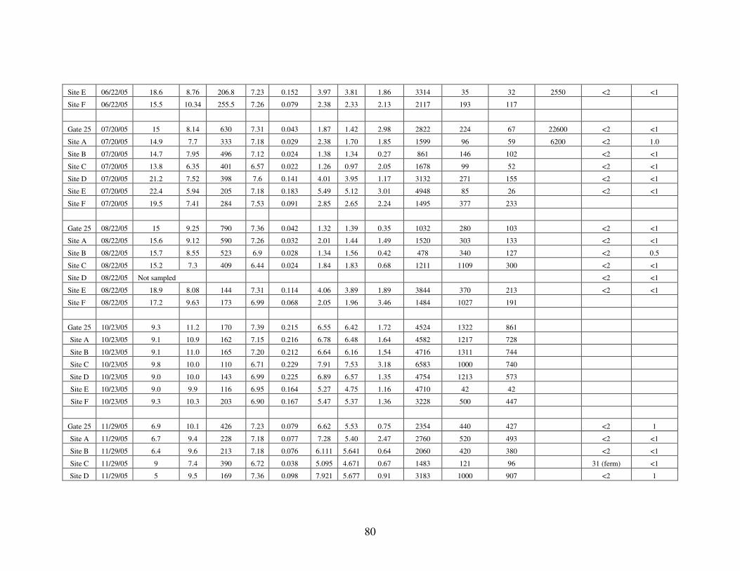
80

Site E 06/22/05 18.6 8.76 206.8 7.23 0.152 3.97 3.81 1.86 3314 35 32 2550 <2 <1 Site F 06/22/05 15.5 10.34 255.5 7.26 0.079 2.38 2.33 2.13 2117 193 117 Gate 25 07/20/05 15 8.14 630 7.31 0.043 1.87 1.42 2.98 2822 224 67 22600 <2 <1 Site A 07/20/05 14.9 7.7 333 7.18 0.029 2.38 1.70 1.85 1599 96 59 6200 <2 1.0 Site B 07/20/05 14.7 7.95 496 7.12 0.024 1.38 1.34 0.27 861 146 102 <2 <1 Site C 07/20/05 13.8 6.35 401 6.57 0.022 1.26 0.97 2.05 1678 99 52 <2 <1 Site D 07/20/05 21.2 7.52 398 7.6 0.141 4.01 3.95 1.17 3132 271 155 <2 <1 Site E 07/20/05 22.4 5.94 205 7.18 0.183 5.49 5.12 3.01 4948 85 26 <2 <1 Site F 07/20/05 19.5 7.41 284 7.53 0.091 2.85 2.65 2.24 1495 377 233 Gate 25 08/22/05 15 9.25 790 7.36 0.042 1.32 1.39 0.35 1032 280 103 <2 <1 Site A 08/22/05 15.6 9.12 590 7.26 0.032 2.01 1.44 1.49 1520 303 133 <2 <1 Site B 08/22/05 15.7 8.55 523 6.9 0.028 1.34 1.56 0.42 478 340 127 <2 0.5 Site C 08/22/05 15.2 7.3 409 6.44 0.024 1.84 1.83 0.68 1211 1109 300 <2 <1 Site D 08/22/05 Not sampled <2 <1 Site E 08/22/05 18.9 8.08 144 7.31 0.114 4.06 3.89 1.89 3844 370 213 <2 <1 Site F 08/22/05 17.2 9.63 173 6.99 0.068 2.05 1.96 3.46 1484 1027 191 Gate 25 10/23/05 9.3 11.2 170 7.39 0.215 6.55 6.42 1.72 4524 1322 861 Site A 10/23/05 9.1 10.9 162 7.15 0.216 6.78 6.48 1.64 4582 1217 728 Site B 10/23/05 9.1 11.0 165 7.20 0.212 6.64 6.16 1.54 4716 1311 744 Site C 10/23/05 9.8 10.0 110 6.71 0.229 7.91 7.53 3.18 6583 1000 740 Site D 10/23/05 9.0 10.0 143 6.99 0.225 6.89 6.57 1.35 4754 1213 573 Site E 10/23/05 9.0 9.9 116 6.95 0.164 5.27 4.75 1.16 4710 42 42 Site F 10/23/05 9.3 10.3 203 6.90 0.167 5.47 5.37 1.36 3228 500 447

Gate 25 11/29/05 6.9 10.1 426 7.23 0.079 6.62 5.53 0.75 2354 440 427 <2 1 Site A 11/29/05 6.7 9.4 228 7.18 0.077 7.28 5.40 2.47 2760 520 493 <2 <1 Site B 11/29/05 6.4 9.6 213 7.18 0.076 6.111 5.641 0.64 2060 420 380 <2 <1 Site C 11/29/05 9 7.4 390 6.72 0.038 5.095 4.671 0.67 1483 121 96 31 (ferm) <1 Site D 11/29/05 5 9.5 169 7.36 0.098 7.921 5.677 0.91 3183 1000 907 <2 1

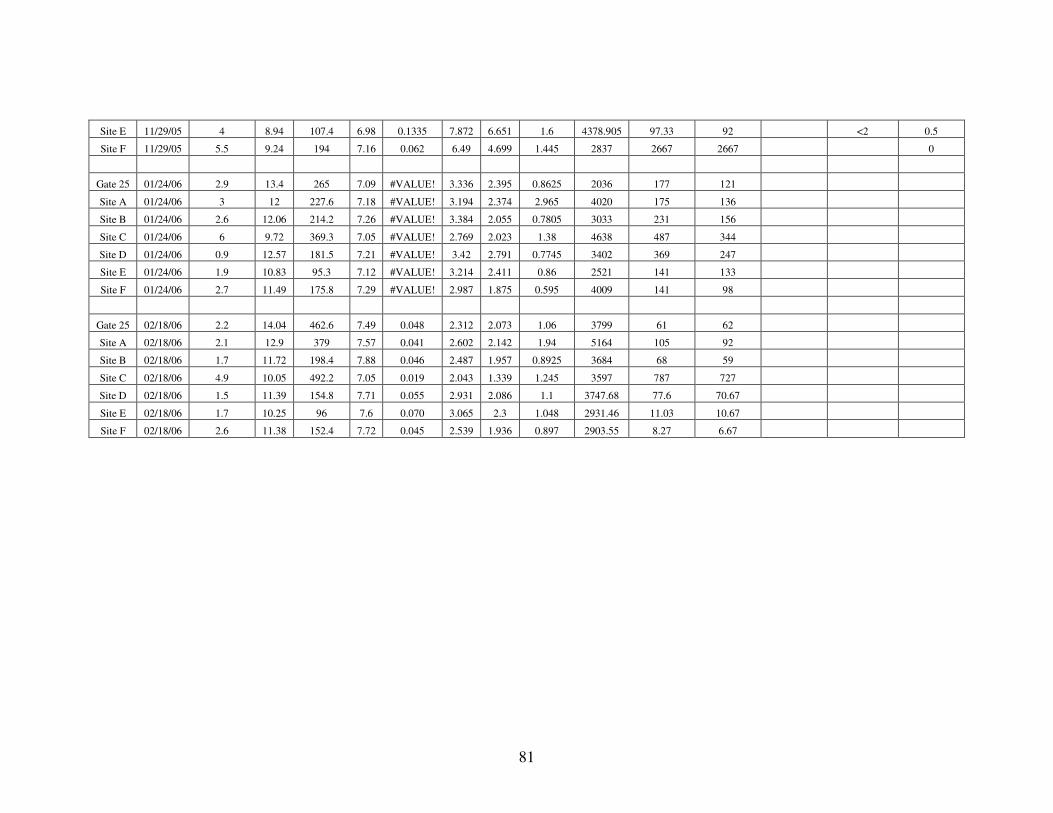
81

Site E 11/29/05 4 8.94 107.4 6.98 0.1335 7.872 6.651 1.6 4378.905 97.33 92 <2 0.5 Site F 11/29/05 5.5 9.24 194 7.16 0.062 6.49 4.699 1.445 2837 2667 2667 0

Gate 25 01/24/06 2.9 13.4 265 7.09 #VALUE! 3.336 2.395 0.8625 2036 177 121 Site A 01/24/06 3 12 227.6 7.18 #VALUE! 3.194 2.374 2.965 4020 175 136 Site B 01/24/06 2.6 12.06 214.2 7.26 #VALUE! 3.384 2.055 0.7805 3033 231 156 Site C 01/24/06 6 9.72 369.3 7.05 #VALUE! 2.769 2.023 1.38 4638 487 344 Site D 01/24/06 0.9 12.57 181.5 7.21 #VALUE! 3.42 2.791 0.7745 3402 369 247 Site E 01/24/06 1.9 10.83 95.3 7.12 #VALUE! 3.214 2.411 0.86 2521 141 133 Site F 01/24/06 2.7 11.49 175.8 7.29 #VALUE! 2.987 1.875 0.595 4009 141 98

Gate 25 02/18/06 2.2 14.04 462.6 7.49 0.048 2.312 2.073 1.06 3799 61 62 Site A 02/18/06 2.1 12.9 379 7.57 0.041 2.602 2.142 1.94 5164 105 92 Site B 02/18/06 1.7 11.72 198.4 7.88 0.046 2.487 1.957 0.8925 3684 68 59 Site C 02/18/06 4.9 10.05 492.2 7.05 0.019 2.043 1.339 1.245 3597 787 727 Site D 02/18/06 1.5 11.39 154.8 7.71 0.055 2.931 2.086 1.1 3747.68 77.6 70.67 Site E 02/18/06 1.7 10.25 96 7.6 0.070 3.065 2.3 1.048 2931.46 11.03 10.67 Site F 02/18/06 2.6 11.38 152.4 7.72 0.045 2.539 1.936 0.897 2903.55 8.27 6.67

82

Appendix B: ANOVA Analyses by Site

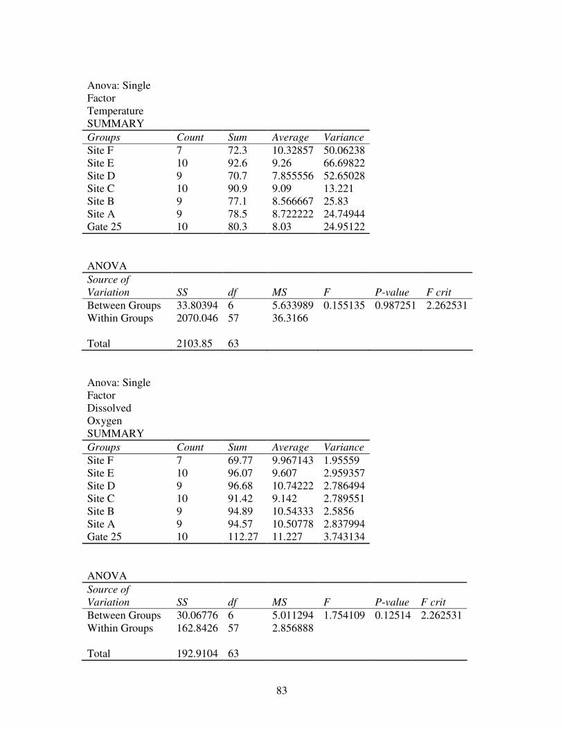
83

Anova: Single Factor Temperature SUMMARY Groups Count Sum Average Variance Site F 7 72.3 10.32857 50.06238 Site E 10 92.6 9.26 66.69822 Site D 9 70.7 7.855556 52.65028 Site C 10 90.9 9.09 13.221 Site B 9 77.1 8.566667 25.83 Site A 9 78.5 8.722222 24.74944 Gate 25 10 80.3 8.03 24.95122 ANOVA Source of Variation SS df MS F P-value F crit Between Groups 33.80394 6 5.633989 0.155135 0.987251 2.262531 Within Groups 2070.046 57 36.3166 Total 2103.85 63

Anova: Single Factor Dissolved Oxygen SUMMARY Groups Count Sum Average Variance Site F 7 69.77 9.967143 1.95559 Site E 10 96.07 9.607 2.959357 Site D 9 96.68 10.74222 2.786494 Site C 10 91.42 9.142 2.789551 Site B 9 94.89 10.54333 2.5856 Site A 9 94.57 10.50778 2.837994 Gate 25 10 112.27 11.227 3.743134 ANOVA Source of Variation SS df MS F P-value F crit Between Groups 30.06776 6 5.011294 1.754109 0.12514 2.262531 Within Groups 162.8426 57 2.856888 Total 192.9104 63

84

Anova: Single Factor Conductivity SUMMARY Groups Count Sum Average Variance Site F 7 1437.2 205.3143 2260.781 Site E 10 1390.5 139.05 2092.605 Site D 9 2132 236.8889 8160.226 Site C 10 4173.4 417.34 32383.87 Site B 9 3143.3 349.2556 30365.11 Site A 9 3192.6 354.7333 22538.83 Gate 25 10 4806.4 480.64 50216.31 ANOVA Source of Variation SS df MS F

P-value F crit

Between Groups 852375.2 6 142062.5 6.404715 3.37E-05 2.262531

Within Groups 1264313 57 22180.93 Total 2116688 63

Anova: Single Factor pH SUMMARY Groups Count Sum Average Variance Site F 7 50.85 7.264286 0.082962 Site E 10 71.52 7.152 0.047662 Site D 9 65.73 7.303333 0.10025 Site C 10 67.94 6.794 0.055804 Site B 9 64.59 7.176667 0.0825 Site A 9 64.53 7.17 0.03195 Gate 25 10 72.15 7.215 0.049406 ANOVA Source of Variation SS df MS F P-value F crit Between Groups 1.621365 6 0.270227 4.28906 0.001236 2.262531 Within Groups 3.591221 57 0.063004 Total 5.212586 63

85

Anova: Single Factor UV SUMMARY Groups Count Sum Average Variance Site F 6 0.5122 0.085367 0.001853 Site E 6 0.8155 0.135917 0.001612 Site D 5 0.6316 0.12632 0.004017 Site C 6 0.3524 0.058733 0.007041 Site B 6 0.41625 0.069375 0.005242 Site A 6 0.4287 0.07145 0.005299 Gate 25 6 0.47055 0.078425 0.004688 ANOVA Source of Variation SS df MS F P-value F crit Between Groups 0.030565 6 0.005094 1.196565 0.331749 2.380311 Within Groups 0.144748 34 0.004257 Total 0.175313 40

Anova: Single Factor TOC SUMMARY Groups Count Sum Average Variance Site F 7 25.216 3.602286 2.84436 Site E 7 33.0965 4.728071 2.727464 Site D 6 29.1035 4.850583 4.068678 Site C 7 22.676 3.239429 6.068962 Site B 7 23.526 3.360857 5.10591 Site A 7 27.1435 3.877643 4.845314 Gate 25 7 24.3025 3.471786 5.231289 ANOVA Source of Variation SS df MS F P-value F crit Between Groups 17.12323 6 2.853872 0.645447 0.693331 2.32977 Within Groups 181.2832 41 4.421541 Total 198.4064 47

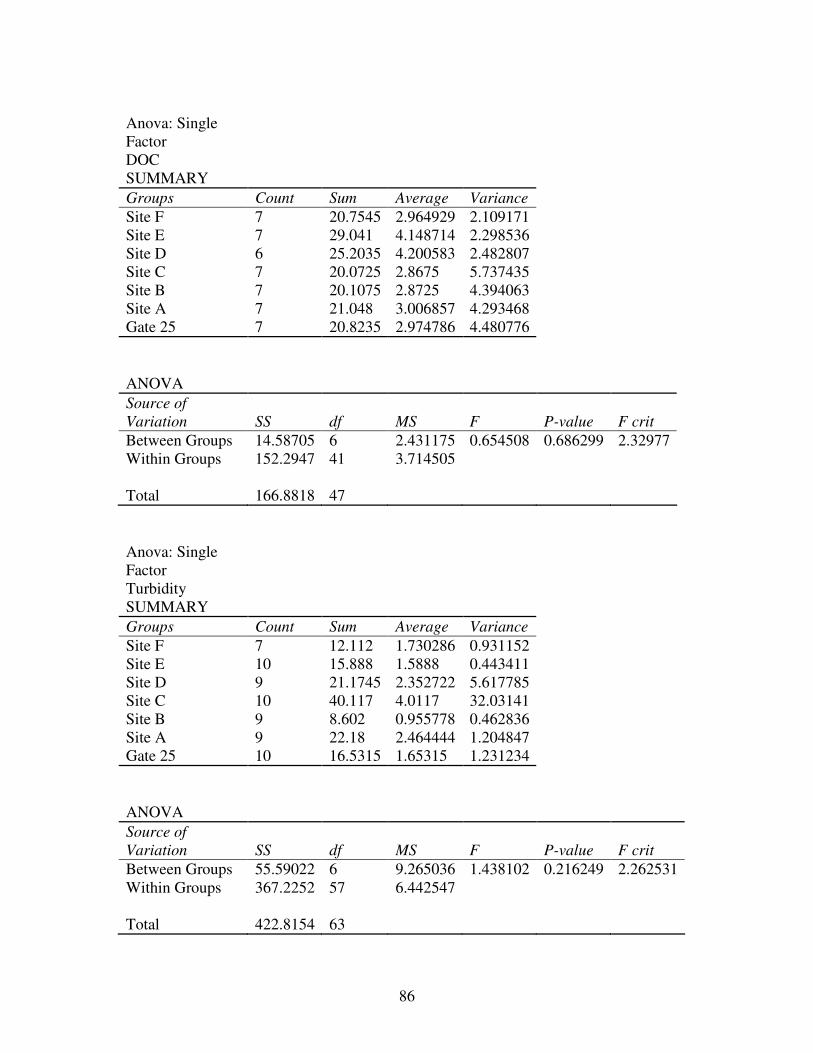
86

Anova: Single Factor DOC SUMMARY Groups Count Sum Average Variance Site F 7 20.7545 2.964929 2.109171 Site E 7 29.041 4.148714 2.298536 Site D 6 25.2035 4.200583 2.482807 Site C 7 20.0725 2.8675 5.737435 Site B 7 20.1075 2.8725 4.394063 Site A 7 21.048 3.006857 4.293468 Gate 25 7 20.8235 2.974786 4.480776 ANOVA Source of Variation SS df MS F P-value F crit Between Groups 14.58705 6 2.431175 0.654508 0.686299 2.32977 Within Groups 152.2947 41 3.714505 Total 166.8818 47

Anova: Single Factor Turbidity SUMMARY Groups Count Sum Average Variance Site F 7 12.112 1.730286 0.931152 Site E 10 15.888 1.5888 0.443411 Site D 9 21.1745 2.352722 5.617785 Site C 10 40.117 4.0117 32.03141 Site B 9 8.602 0.955778 0.462836 Site A 9 22.18 2.464444 1.204847 Gate 25 10 16.5315 1.65315 1.231234 ANOVA Source of Variation SS df MS F P-value F crit Between Groups 55.59022 6 9.265036 1.438102 0.216249 2.262531 Within Groups 367.2252 57 6.442547 Total 422.8154 63

87

Anova: Single Factor Particles SUMMARY Groups Count Sum Average Variance Site F 7 18073.61 2581.944 871249.2 Site E 7 26648.18 3806.882 851346.6 Site D 6 27061.02 4510.169 4861006 Site C 7 20598.38 2942.625 4272618 Site B 7 15740.96 2248.709 2608218 Site A 7 21641.71 3091.672 2230845 Gate 25 7 17894.27 2556.324 1605707 ANOVA Source of Variation SS df MS F P-value F crit Between Groups 24596568 6 4099428 1.698688 0.145819 2.32977 Within Groups 98944938 41 2413291 Total 1.24E+08 47

Anova: Single Factor Fecal Coliforms SUMMARY Groups Count Sum Average Variance Site F 7 4912.61 701.8014 861235.9 Site E 10 1254.3 125.43 24683.02 Site D 9 3843.82 427.0911 176356 Site C 10 9010.37 901.037 2026228 Site B 9 3091.223 343.4692 159075 Site A 9 3226.034 358.4482 145443 Gate 25 10 3748.516 374.8516 159778.9 ANOVA Source of Variation SS df MS F P-value F crit Between Groups 3769113 6 628185.6 1.238527 0.300544 2.262531 Within Groups 28910614 57 507203.7 Total 32679727 63

88

Anova: Single Factor E. coli SUMMARY Groups Count Sum Average Variance Site F 7 3759.11 537.0157 901011.5 Site E 10 1021.61 102.161 19290.01 Site D 9 2746.34 305.1489 88797.06 Site C 10 7559.11 755.911 2088671 Site B 9 2125.91 236.2122 61648.46 Site A 9 2374.474 263.8304 75632.19 Gate 25 10 2569.616 256.9616 98908.58 ANOVA Source of Variation SS df MS F P-value F crit Between Groups 2793796 6 465632.7 0.980224 0.447136 2.262531 Within Groups 27076520 57 475026.7 Total 29870316 63

89

Appendix C: ANOVA Analyses by Season

90

Anova: Single Factor Temperature SUMMARY Groups Count Sum Average Variance Spring 12 87.4 7.283333 8.028788 Summer 20 320.1 16.005 8.466816 Winter 18 46.8 2.6 1.938824 Fall 14 108.1 7.721429 3.666429 ANOVA Source of Variation SS df MS F

P-value F crit

Between Groups 1774.04 3 591.3468 107.5796 4.15E-24 2.758078

Within Groups 329.8097 60 5.496829 Total 2103.85 63

Anova: Single Factor DO SUMMARY Groups Count Sum Average Variance Spring 12 137.12 11.42667 0.528515 Summer 20 169.84 8.492 1.554048 Winter 18 211.29 11.73833 1.438956 Fall 14 137.42 9.815714 0.936196 ANOVA Source of Variation SS df MS F

P-value F crit

Between Groups 120.937 3 40.31234 33.60604 7.14E-13 2.758078

Within Groups 71.97338 60 1.199556 Total 192.9104 63

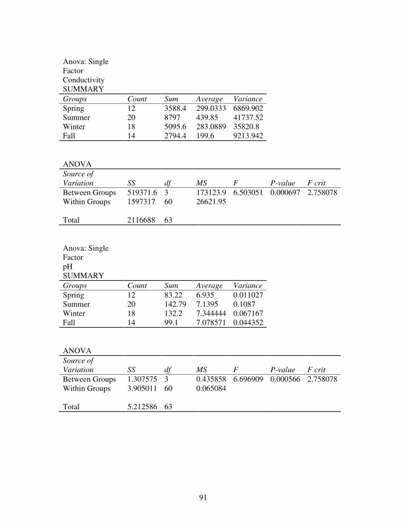
91

Anova: Single Factor Conductivity SUMMARY Groups Count Sum Average Variance Spring 12 3588.4 299.0333 6869.902 Summer 20 8797 439.85 41737.52 Winter 18 5095.6 283.0889 35820.8 Fall 14 2794.4 199.6 9213.942 ANOVA Source of Variation SS df MS F P-value F crit Between Groups 519371.6 3 173123.9 6.503051 0.000697 2.758078 Within Groups 1597317 60 26621.95 Total 2116688 63

Anova: Single Factor pH SUMMARY Groups Count Sum Average Variance Spring 12 83.22 6.935 0.011027 Summer 20 142.79 7.1395 0.1087 Winter 18 132.2 7.344444 0.067167 Fall 14 99.1 7.078571 0.044352 ANOVA Source of Variation SS df MS F P-value F crit Between Groups 1.307575 3 0.435858 6.696909 0.000566 2.758078 Within Groups 3.905011 60 0.065084 Total 5.212586 63

92

Anova: Single Factor UV SUMMARY Groups Count Sum Average Variance Summer 20 1.3119 0.065595 0.002493 Winter 7 0.32425 0.046321 0.000236 Fall 14 1.99105 0.142218 0.004861 ANOVA Source of Variation SS df MS F

P-value F crit

Between Groups 0.063344 2 0.031672 10.74894 0.0002 3.244821 Within Groups 0.111969 38 0.002947 Total 0.175313 40

Anova: Single Factor TOC SUMMARY Groups Count Sum Average Variance Summer 20 47.573 2.37865 1.502189 Winter 14 44.608 3.186286 0.050892 Fall 14 92.883 6.6345 0.860913 ANOVA Source of Variation SS df MS F

P-value F crit

Between Groups 158.0114 2 79.00568 88.01214 2.8E-16 3.20432

Within Groups 40.39506 45 0.897668 Total 198.4064 47

93

Anova: Single Factor DOC SUMMARY Groups Count Sum Average Variance Summer 20 43.6685 2.183425 1.45332 Winter 14 31.848 2.274857 0.089363 Fall 14 81.534 5.823857 0.71687 ANOVA Source of Variation SS df MS F

P-value F crit

Between Groups 128.7877 2 64.39384 76.06749 3.67E-15 3.20432

Within Groups 38.0941 45 0.846536 Total 166.8818 47

Anova: Single Factor Turbidity SUMMARY Groups Count Sum Average Variance Spring 12 52.53 4.3775 23.42922 Summer 20 41.375 2.06875 3.726734 Winter 18 22.28 1.237778 0.390505 Fall 14 20.42 1.458571 0.486005 ANOVA Source of Variation SS df MS F P-value F crit Between Groups 81.32935 3 27.10978 4.763261 0.004809 2.758078 Within Groups 341.486 60 5.691434 Total 422.8154 63

94

Anova: Single Factor Particles SUMMARY Groups Count Sum Average Variance Summer 20 46019.67 2300.984 3630748 Winter 14 49486.4 3534.743 675180 Fall 14 52152.04 3725.145 1917020 ANOVA Source of Variation SS df MS F P-value F crit Between Groups 20858695 2 10429348 4.570586 0.015592 3.20432 Within Groups 1.03E+08 45 2281840 Total 1.24E+08 47

Anova: Single Factor Fecal Coliforms SUMMARY Groups Count Sum Average Variance Spring 12 8210 684.1667 1754216 Summer 20 6030 301.5 81071.32 Winter 18 2975.903 165.3279 40480.8 Fall 14 11870.97 847.9264 490887.3 ANOVA Source of Variation SS df MS F P-value F crit Between Groups 4773291 3 1591097 3.420925 0.022793 2.758078 Within Groups 27906436 60 465107.3 Total 32679727 63

95

Anova: Single Factor E. coli SUMMARY Groups Count Sum Average Variance Spring 12 8210 684.1667 1754216 Summer 20 2361 118.05 5508.997 Winter 18 2388.19 132.6772 29604.67 Fall 14 9196.98 656.9271 413993.2 ANOVA Source of Variation SS df MS F P-value F crit Between Groups 4584081 3 1528027 3.625752 0.017916 2.758078 Within Groups 25286235 60 421437.3 Total 29870316 63

96

Appendix D: Binary ANOVA Analysis by Site

97

Anova: Single Factor Conductivity SUMMARY Groups Count Sum Average Variance Site F 7 0 0 0 Site E 10 7 0.7 0.233333 Site D 10 1 0.1 0.1 Site C 10 3 0.3 0.233333 Site B 9 2 0.222222 0.194444 Site A 9 0 0 0 Gate 25 10 4 0.4 0.266667 ANOVA Source of Variation SS df MS F P-value F crit Between Groups 3.498291 6 0.583048 3.734372 0.003297 2.259605 Within Groups 9.055556 58 0.15613 Total 12.55385 64

Anova: Single Factor Turbidity SUMMARY Groups Count Sum Average Variance Site F 7 0 0 0 Site E 10 0 0 0 Site D 10 1 0.1 0.1 Site C 10 2 0.2 0.177778 Site B 9 0 0 0 Site A 9 1 0.111111 0.111111 Gate 25 10 0 0 0 ANOVA Source of Variation SS df MS F P-value F crit Between Groups 0.364957 6 0.060826 1.041026 0.408489 2.259604 Within Groups 3.388889 58 0.058429 Total 3.753846 64

98

Anova: Single Factor Fecal Coliforms SUMMARY Groups Count Sum Average Variance Site F 7 4 0.571429 0.285714 Site E 10 2 0.2 0.177778 Site D 10 6 0.6 0.266667 Site C 10 6 0.6 0.266667 Site B 9 5 0.555556 0.277778 Site A 9 4 0.444444 0.277778 Gate 25 10 6 0.6 0.266667 ANOVA Source of Variation SS df MS F P-value F crit Between Groups 1.287424 6 0.214571 0.831962 0.550152 2.259604 Within Groups 14.95873 58 0.257909 Total 16.24615 64

Anova: Single Factor E. coli SUMMARY Groups Count Sum Average Variance Site F 7 4 0.571429 0.285714 Site E 10 3 0.3 0.233333 Site D 10 6 0.6 0.266667 Site C 10 6 0.6 0.266667 Site B 9 5 0.555556 0.277778 Site A 9 5 0.555556 0.277778 Gate 25 10 3 0.3 0.233333 ANOVA Source of Variation SS df MS F P-value F crit Between Groups 1.087424 6 0.181237 0.693446 0.655786 2.259604 Within Groups 15.15873 58 0.261357 Total 16.24615 64

99

Anova: Single Factor SUVA SUMMARY

Groups Count Sum Average Variance Site F 8 5 0.625 0.267857 Site E 8 6 0.75 0.214286 Site D 8 3 0.375 0.267857 Site C 8 3 0.375 0.267857 Site B 8 3 0.375 0.267857 Site A 8 3 0.375 0.267857 Gate 25 8 5 0.625 0.267857 ANOVA Source of Variation SS df MS F P-value F crit Between Groups 1.25 6 0.208333 0.800654 0.574166 2.290435 Within Groups 12.75 49 0.260204 Total 14 55

100

Appendix D: Binary ANOVA Analysis by Season

101

Anova: Single Factor Conductivity SUMMARY Groups Count Sum Average Variance Spring 12 1 0.083333 0.083333 Summer 20 9 0.45 0.260526 Winter 18 6 0.333333 0.235294 Fall 14 4 0.285714 0.21978 ANOVA Source of Variation SS df MS F P-value F crit Between Groups 1.02619 3 0.342063 1.613024 0.195783 2.758078 Within Groups 12.72381 60 0.212063 Total 13.75 63

Anova: Single Factor Turbidity SUMMARY Groups Count Sum Average Variance Spring 12 2 0.166667 0.151515 Summer 20 2 0.1 0.094737 Winter 18 0 0 0 Fall 14 0 0 0 ANOVA Source of Variation SS df MS F P-value F crit Between Groups 0.283333 3 0.094444 1.634615 0.190844 2.758078 Within Groups 3.466667 60 0.057778 Total 3.75 63

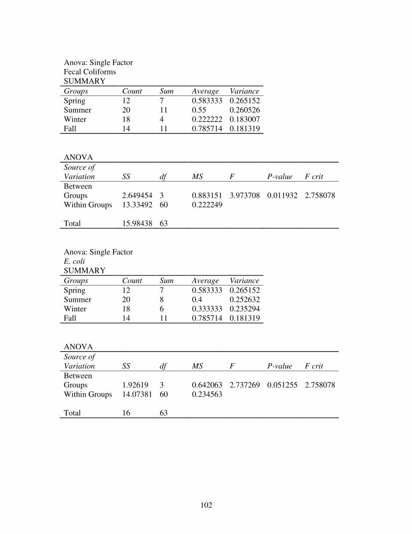
102

Anova: Single Factor Fecal Coliforms SUMMARY Groups Count Sum Average Variance Spring 12 7 0.583333 0.265152 Summer 20 11 0.55 0.260526 Winter 18 4 0.222222 0.183007 Fall 14 11 0.785714 0.181319 ANOVA Source of Variation SS df MS F P-value F crit Between Groups 2.649454 3 0.883151 3.973708 0.011932 2.758078 Within Groups 13.33492 60 0.222249 Total 15.98438 63

Anova: Single Factor E. coli SUMMARY Groups Count Sum Average Variance Spring 12 7 0.583333 0.265152 Summer 20 8 0.4 0.252632 Winter 18 6 0.333333 0.235294 Fall 14 11 0.785714 0.181319 ANOVA Source of Variation SS df MS F P-value F crit Between Groups 1.92619 3 0.642063 2.737269 0.051255 2.758078 Within Groups 14.07381 60 0.234563 Total 16 63

103

Anova: Single Factor SUVA SUMMARY Groups Count Sum Average Variance Summer 20 16 0.8 0.168421 Winter 7 5 0.714286 0.238095 Fall 14 8 0.571429 0.263736 ANOVA Source of Variation SS df MS F P-value F crit Between Groups 0.430662 2 0.215331 1.015568 0.371816 3.244821 Within Groups 8.057143 38 0.21203 Total 8.487805 40