monash.edu/ business-economics

ABN 12 377 614 012 CRICOS Provider No. 00008C

© 2018 Lata Gangadharan, Philip J. Grossman, Mana Komai and Joe Vecci All rights reserved. No part of this paper may be reproduced in any form, or stored in a retrieval system, without the prior written permission of the author.

Department of Economics

ISSN number 1441-5429

Discussion number 01/18

Impact of Social Identity and Inequality on Antisocial Behaviour

Lata Gangadharan1, Philip J. Grossman2, Mana Komai3 and Joe Vecci4

Abstract: Antisocial behaviour can be observed in response to social comparisons with advantaged others.

This paper uses a laboratory experiment to examine if social group affiliation mitigates or

increases antisocial behaviour in the presence of inequality. While research has documented the

harmful effects of inequality, less is known about how social identity may interact with income

inequality to influence antisocial behaviour. In our experiment, participants play a modified

version of an investment game in which they can reduce others’ payoff at a cost to themselves.

Participants are identified by their income groups and/or social groups. We use naturally

occurring, exogenous social groups to capture social identity and vary the combination of

income identity and social identity. We find little difference in rates of antisocial behaviour

across the environments. However, in a setting with revealed social identity and income identity

we observe a redirection in antisocial behaviour relative to a setting in which social identity is

not revealed. We find that low income participants are more likely to be antisocial towards

someone from a different income or social group. In contrast, high income participants do not

vary their behaviour. The targeting of antisocial behaviour by low income individuals is

consistent with our theoretical framework and suggests that identity politics causes low income

people who are already in conflict with one another to shift their blame culturally. Our findings

suggest that the context in which inequality exists may have important effects on antisocial

behaviour.

Keywords: Social Identity, Income inequality, Antisocial behaviour, Experiment, Natural groups

JEL Codes: C91, D003, D6

1 Monash University, Lata.Gangadharan@monash.edu 2 Monash University, Philip.Grossman@monash.edu; Rasmuson Chair, University of Alaska Anchorage 3 St Cloud State, mkomai@stcloudstate.edu 4 Gothenburg University, joseph.vecci@gu.se

Acknowledgements: Gangadharan, Grossman, and Komai acknowledge financial support from the Australian Research Council

(Discovery Project DP1411151). Vecci acknowledges support from the Swedish Research Council (Project no. 348-2014-4030).

We are grateful to Rick Wilson for all of his help facilitating this project. We wish to thank audiences at Economic Science

Association Meetings, Universitat Autònoma de Barcelona, University of Alaska Anchorage, and ANSWEE meetings for

insightful comments and suggestions.

2

1. Introduction

Antisocial behaviour can negatively affect a society by constantly threatening the security

and cohesion of communities, undermining the well-being and advancement of both the victims

as well as the perpetrators, and discouraging investment and business practices. It is therefore

important to investigate sources, targets, intensity, and patterns of antisocial behaviour.5

Social differences, such as those generated by income inequality, may exacerbate antisocial

behaviour (Alesina and Perotti, 1996; Steward, 2001).6 This has become more pertinent in

recent times as income inequality increases in many countries along with a growing concern

that high levels of inequality may trigger social unrest (Piketty, 2014).7

The social structure of a society, such as the proportion of different social groups, may

affect the intensity and the pattern of antisocial behaviour caused by income inequality. An

important differentiation between peaceful and violent societies is the degree of inequality

between social groups (Steward, 2001). In societies in which social groups have unequal

access to economic resources (e.g., North and South Sudanese in Sudan8, Tutsis and Hutus in

Rwanda, or White and African Americans in the United States), economic inequalities,

coinciding with cultural/social differences, may make social identity a strong unifying source

that may lead, and has led, to conflict and sporadic violent outbursts over the distribution of

resources. In contrast, when inequality does not correlate with social groups, social identity

may play a muting role in conflict and antisocial behaviour. Alternatively, this setting could

also lead to greater antisocial behaviour, as there are more combinations of social groups to

target.

These examples suggest an important interaction between shared identities based on social

characteristics and economic markers. Investigating such interaction is an important focus of

our paper. We study, experimentally, if social identity influences the intensity and/or patterns

5 Several recent papers have shown that individuals are motivated by antisocial preferences and that they destroy

or burn others’ wealth at a cost to themselves (for example, Zizzo and Oswald, 2001; Zizzo, 2003; Abbink and

Sadrieh, 2009; Abbink and Herrmann, 2011). These kinds of antisocial behaviour appear to have an envious or

spiteful streak and seem to be mainly directed at the wealthy (Gino and Pierce, 2009a 2009b; Cason et al., 2002b);

those of high status (Cikara and Fiske, 2013); those who are first movers and have the power to take (Bosman and

van Winden, 2002; Bosman et al., 2006; Albert and Mertins, 2008); a high income beneficiary (Beckman et al.,

2002); or high ranking subjects in a public good game (Saijo and Nakamura, 1995; Cason et al., 2002a). 6 See for instance Gurr (1993) and Sen (1973) for a discussion. Alesina and Perotti (1996) argue that inequality

reduces growth through political instability and conflict. 7 Evidence of this can be found in the Occupy movements in many countries including the United States and

Australia. 8 Conflict between the South Sudan’s predominantly Christian population and the North’s predominantly Muslim

population over resource distribution (among other factors) led to the creation of the nation of South Sudan in

2011.

3

of antisocial behaviour in a state of inequality. Two distinct group identities are introduced: a

randomly assigned income identity based on participants’ access to resources, and a naturally

formed social identity based on participants’ affiliation to their university residential college.

A unique college assignment policy allows us to exploit the natural, yet exogenous, social

identity of our participants.9

Our participants interact in three different environments distinguished by two main

characteristics: a) if information about participants’ affiliation to a particular group is common

knowledge, and b) if the two group identities overlap (i.e., whether participants with the same

income identity are also affiliated with the same social identity). In the first environment, we

explore the situation where participants’ affiliation to both groups is public information and

income inequality overlaps with social affiliation, termed “socially embedded inequality.” It

commonly occurs when income differences closely parallel social and cultural (ethnic,

linguistic or racial) characteristics (Mogues and Carter, 2005). Such environments are

reflective of the income gap between African Americans and other racial groups in the United

States.10 In the second environment, participants’ affiliation to both groups is public

information but income indenity does not completely overlap with social identity. In this

environment, groups are mixed, in the sense that each social group contains both high and low

income group members. We compare the first and second environment to our third

environment, in which participants are explicitly identified by their income identities but

information about their social identities is not public.

Within each environment, we implement a two-stage, multiperiod saving/investment game.

The first stage creates and reinforces income differences between participants. Participants are

randomly chosen to have high income or low income (income identity). Participants are given

the opportunity to invest or save their endowment. High (low) income participants are

characterized by a larger (smaller) initial endowment and a higher (lower) rate of return to their

investment. Earnings are observable to all participants. The second stage introduces an

additional option — participants can reduce the earnings of another participant at a personal

cost. This stage is designed to observe the existence, intensity, and pattern of participants’

antisocial behaviour. Such financially vindictive behaviour can be potentially harmful to

9 As described in Section 2.1, upon commencement at college, our Rice University subjects are randomly assigned

to one of eleven residential colleges. Students participate in activities (including a week-long orientation) designed

to build college loyalty and to immerse students into the traditions and culture of their colleges. Participants in

our experiment have a strong sense of belonging to their colleges. 10 As discussed in Steward (2001) evidence of embedded inequality is prevalent in both developing and developed

countries. She argues it is both pervasive and underacknowledged but it is particularly severe in Latin and Central

America (see also Figueroa et al., 1996).

4

innovation and the functioning of competitive markets and would likely impede economic

growth.

To motivate our experimental design, we develop a stylized theoretical model, in which

individuals have affiliations to both an income group and to a social group. Our main focus is

on the observed antisocial behaviour and how it varies across our three environments. We

hypothesize that we will observe less antisocial behaviour within income groups in the

environment in which income and social identities overlap relative to settings where social

identity is mixed across income groups or social identity is not public. We also hypothesize

that antisocial behaviour across income types is lowest when social and income identities are

mixed relative to the other environments.

Findings from the experiment show no evidence that antisocial behaviour differs in an

environment with socially embedded inequality relative to an environment in which social

identity is mixed across income groups. On the other hand, we find that for participants with

low income identity, both environments with revealed social identity have lower rates of

antisocial behaviour relative to a setting where social identity is not revealed. Strikingly, low

income participants direct more antisocial behaviour towards other low income participants in

the environment where social identity is not revealed relative to settings with revealed social

identity. This suggests that inequality research that ignores social identity may overestimate

the impact of inequality on behaviour. In contrast, the combination of income and social

identity has little influence on the intensity of antisocial behaviour of high income participants.

We also find that while low income participants direct antisocial behaviour towards other low

income group members, they target predominately those from outside their social identity. This

targeting of antisocial behaviour is consistent with the model and suggests that identity politics

causes low income people who are already in conflict with one another to shift their blame

culturally.

Our research offers contributions in three domains. First, there are few papers that attempt

to bridge the literature between social identity and inequality and these papers are

predominately theoretical.11 For example, Esteban and Ray (1994) and Duclos et al. (2004)

posit a theoretical model that contrasts a conventional inequality measure based on wealth

11 The only exception is Weng and Carlsson (2015) who use a public goods task to compare the impact of group

identity and peer punishment on cooperation under heterogenous and homogenous income distributions. They

find that without punishment social identity improves cooperation in heterogeneous groups. On the other hand,

the effectiveness of punishment on cooperation depends on the task used to induce group identity. Our paper

differs not only in terms of the outcome under study, but also in terms of the inherent question of the research.

Unlike Weng and Carlsson (2015), we compare different environments under which social identity may interact

with income inequality.

5

differences with their economic polarization measure based on differences across groups. They

examine a setup in which groups are highly polarized, but individuals are homogenous within

groups and predict that as groups become more polarized, even as inequality decreases, conflict

increases.12 Mogues and Carter (2005) extend this model by endowing individuals with two

characteristics, a social identity based on ethnicity and, similar to Esteban and Ray (1994), an

income identity based on wealth. The authors argue that economic (i.e., income) inequality

may be more persistent when it is socially embedded. They show that higher economic and

social polarization increases income and wealth inequality. In a similar vein, Robinson (2001)

extends a rational choice model of conflict to investigate how inequality impacts conflict when

social groups comprise both capitalists and workers. He finds that if social groups contain only

workers or capitalists (i.e., inequality is socially embedded) then growth in inequality leads to

more conflict. Unlike Mogues and Carter (2005) he also finds that if social groups contain a

similar balance of both capitalists and workers then conflict is independent of inequality. We

build on these theoretical studies by empirically comparing different environments in which

income identity and social identity may interact, including an environment that reproduces

socially embedded income inequality and an environment in which social groups are mixed

across income groups. Individuals do not act in isolation but make decisions as part of a social

group. Hence to explain the prevalence of antisocial behaviour in complex societies, we need

to understand how individuals interact in environments with income inequality and different

social groups.

Second, studies that investigate the impact of heterogenous income groups generally find

that high income subjects behave differently from low income subjects. Low income subjects

have been shown to cooperate relatively more than high income subjects (Buckley and Croson,

2006; van Dijk et al., 2002), while other studies have shown that low income subjects are as

willing as their high income counterparts to harm others at a cost to themselves (Grossman and

Komai, 2016). This mixed evidence suggests that the impact of income inequality on behaviour

is highly heterogeneous. Moreover, what is yet unexplored is how the inclusion of social

identity in a setting with income inequality affects behaviour, and in particular the behaviour

of low income and high income individuals, and whether socially embedded inequality

differentially affects this behaviour. Our experimental design allows us to examine this

heterogeneity of behaviour.

12 For instance, there may be local equalization of incomes at different ends of the income distribution; this will

increase polarization across income groups, but reduce inequality.

6

Third, our paper contributes to the relatively small, yet growing, literature on natural,

exogenously determined social identity.13 Participants’ social identity is formed based on

participants’ randomly allocated university residential arrangements. This exogenous

assignment of social identity helps us abstract from selection bias, as students cannot choose

which college to reside in based on social, cultural, or political preferences. Moreover, unlike

many experimental studies in which social identity is artificially created using the minimal group

paradigm (Chen and Li, 2009), using participants’ university residential arrangements

introduces a “naturally formed social identity.”14 When social identity is induced in the lab, it

is possible that participants may not accept the assigned social group, and even if they do,

affiliation with the social group may be weak or perhaps prone to experimenter demand effects

leading to misestimation of the true effect of social identity on behaviour. Our naturally formed

social identity can help avoid such concerns.

2. Experimental Design

2.1 Setting

The experiment was conducted at Rice University and participants were recruited from the

university’s residential colleges. Rice University has a unique residential college system. Upon

commencement at college, all undergraduate students are randomly assigned to one of eleven

colleges.15 Each college has its own dorms, academic advisors, and dining hall. Three-quarters

of Rice’s 3,700 undergraduate students study, eat, socialize, and sleep in the same environment

for all of their four years at Rice. Each college is independently governed by faculty, alumni,

and students and has its own budget supporting social events, resources, and facilities. The

interaction between past and present students encourages distinct college norms and traditions.

As members of a college, students engage in many different college-oriented activities, in

addition to a university-wide college orientation, designed to immerse students in their

college’s traditions and culture. College teams also compete in numerous sporting and social

activities, further accentuating the students’ college affiliation.

We argue that the social identity of our participants is based on residential college specific

identity rather than other kinds of preferences (such as political or social). We establish the

strength of our participants’ college identity by using two different approaches. First, we

13 Lane (2016) provides a meta-analysis of natural and artificially induced social identities. 14 Goette et al. (2006) is a notable exception. The authors use the random allocation of soldiers to platoons to

study cooperation. This study does not investigate the interaction between income inequality and social identity. 15 The average size of a residential college is 350 undergraduates.

7

surveyed 263 Rice University students and asked them to respond (on a 4-point Likert scale)

to five statements relating to their knowledge of and connection to their college.16 Between 80-

84% reported that they Strongly Agree or Agree with these statements. Second, in a post-

experiment survey of our participants (n= 186), 75% of respondents said they were either very

proud or proud to be associated with their college. As expected, college affiliation also appears

to be strongly associated with friendship groups: 46% of respondent’s report that all their

closest university friends are from their college.

2.2 Procedure

Recruitment of subjects took place via emails distributed to all students within a residential

college and flyers distributed in dining halls and dorm rooms at lunch and dinner times. All

subjects were inexperienced, i.e., they had never previously participated in an experiment with

features similar to the one reported in this paper. In total, 186 subjects participated in 16

sessions. Within each session we invited students from four colleges.17 Subjects were neither

informed of the number of colleges used within a session nor the number of college subjects

within each session.

Subjects were informed that the session was comprised of multiple stages and that

instructions would be provided and explained before each stage began. At the start of a stage,

subjects were provided a hard copy of the instructions for that stage and these were read aloud

by the experimenter to establish common knowledge among all subjects. A summary of the

instructions with payoff information was also provided on the computer through Z-tree

(Fischbacher, 2007) which subjects read at their own pace.

We used a between-subject design and stages 1 and 2 (explained in detail below) focused

on a single environment containing two, six-person fixed groups.18 Each group of six contained

three subjects from each of two colleges. In stage 3, subjects played a three-person, single-shot

linear public good game. Finally, subjects were administered a survey to collect demographics

such as gender, age and major. The survey also included questions on subjects’ perceptions

about their colleges and their friendship networks within and across colleges. Subject earnings

averaged US$ 27.74, with an interquartile range of $23.50 to $34.50. Sessions lasted about 90

minutes on average, including the time taken for instructions and payment distribution.

16 Questions asked were: “I have spent time trying to find out more about <college>, such as its history, traditions,

and customs”; “I have a strong sense of belonging to <college>”; “In order to learn more about <college>, I have

often talked to other people about <college>”; “I have a lot of pride in <college> and its accomplishments”; “I

feel good about <college>.” We would like to thank Rick Wilson for conducting this survey. 17 In total, six colleges were selected to ensure a diverse distribution of colleges and to allow for a large sample. 18 Due to low turnout, one session was conducted with six subjects (one group).

8

2.3 Decision Making

In stages 1 and 2, subjects interact in fixed groups of six. In stage 1, all subjects take part

in an investment task for 10 rounds. Subjects are randomly assigned an income identity: high

income versus low income subjects. High income (low income) subjects are known as Type A

(B) subjects during the experiment. In the paper, we refer to high income as HI and low income

as LI. HI subjects have endowments twice that of the LI subjects (60 versus 30 cents,

respectively) and higher expected returns from investing (25% versus 20%, respectively). In

each round, subjects choose to save or invest their endowments. Investment has a 50%

probability of success. If the investment is successful, HI subjects receive 120 cents and the LI

subjects receive 52 cents. If the investment is not successful, HI and LI subjects receive 30 and

20 cents, respectively. At the end of each round, that round’s earnings and cumulative earnings

of all the subjects are displayed on the screen, along with their types. This stage is intended to

create and reinforce income differences between the two types of subjects.

In stage 2, subjects participate in 20 rounds identical to stage 1, except subjects now also

have the option to attack (reduce the earnings of) anyone in their group at a cost to themselves.

In each round of stage 2, subjects must make two decisions. The first decision is whether they

would like to attack a specific subject or no-one. They can only attack one subject per period.

It costs the perpetrator 5 cents to attack and the victim’s earnings are reduced by 20 cents.

Whether multiple perpetrators or one perpetrator, the victim’s earnings were reduced by only

20 cents. When deciding to attack, subjects are also shown a table that contains information

regarding each subjects’ previous period’s earnings, each subjects’ cumulative earnings, and

own payoff consequences for any action taken (see Table 2). Their second decision is whether

to save or invest the remaining endowment. Stage 2 allows us to examine whether subjects

engage in antisocial behaviour. As in stage 1, subjects receive complete information regarding

all subjects’ previous period’s earnings and all subjects’ cumulative earnings (see Table 2).

Subjects were not informed whether other subjects attacked and/or who was the target of such

behaviour.19

3. Experimental Environments

Prior to stage 1, subjects are asked to select their residential colleges from a list provided.

This allows us to introduce a social identity. We introduce three environments: “Common,”

19 In stage 3, all subjects take part in a three-person, one-shot voluntary contribution mechanism game. The

decision whether to contribute to the public good is made within type. In other words, subjects are grouped with

HI members if they are HI, and LI members if they are LI.

9

“Mixed,” and “Random.” In all three environments, each group of six was comprised of three

students from each of two colleges. Three subjects were designated HI and three were

designated LI.

In the Common environment, inequality is socially embedded; the two identities

completely overlap and subjects’ affiliation to both identity groups is public information. In

the Mixed environment, the two identities do not overlap, but subjects’ affiliation to both

identity groups is public information. Within each group of six, each income subgroup

contained two subjects from the same college and one person from another. The Mixed

environment group composition implies that within each income group a subject has the option

of attacking a subject from their own social group or a subject from outside their social group.

In the Random environment, subjects are explicitly identified by their income type but

information about their social identity is not public. A summary of the environments can be

found in Table 1. Subjects participate in only one environment.

In both the Common and Mixed environments, subjects’ social and income identities, round

earnings, and cumulative earnings were displayed in the payment table at the end of a round.

In the Random environment, the end-of-round feedback was similar with the only exception

that information about subjects’ social identity was not provided.

3.1 Theoretical Framework and Hypotheses

3.1.1 Basic model

In this section we describe the theoretical framework that we draw on to develop the

testable hypotheses.

Let 𝑆 = {1, … , 𝐼} denote the set of individuals, and 𝑥 = (𝑥1, … , 𝑥𝐼) the resource (i.e.,

income) allocation among them. Consider the following utility function for individual 𝑖:

𝑈𝑖(𝑥) = 𝑥𝑖 + ∑ 𝜌𝑖𝑗

𝑖≠𝑗

(𝑥𝑖 − 𝑥𝑗) 𝑖 ≠ 𝑗

Antisocial behaviour can be supported when 𝜌𝑖𝑗 > 0. 𝜌𝑖𝑗 > 0 implies that 𝜕𝑈𝑖(𝑥)

𝜕𝑥𝑖= 1 +

∑ 𝜌𝑖𝑗𝑖≠𝑗 > 0, and 𝜕𝑈𝑖(𝑥)

𝜕𝑥𝑗= −𝜌𝑖𝑗 < 0. These two inequalities suggest respectively that increases

in own income increase i’s utility, while increases in the incomes of other subjects decrease it.

Prosocial behaviour can be supported when 𝜌𝑖𝑗 < 0 𝑎𝑛𝑑 |∑ 𝜌𝑖𝑗𝑖≠𝑗 | < 1, implying that both

increases in own and other’s income increase i’s utility.

We assume that 𝜌𝑖𝑗 (𝑥𝑖 , 𝑥𝑗): 𝑅2 → 𝑅, 𝜕𝜌𝑖𝑗(𝑥𝑖,𝑥𝑗)

𝜕𝑥𝑖< 0, and

𝜕𝜌𝑖𝑗(𝑥𝑖,𝑥𝑗)

𝜕𝑥𝑗> 0. These assumptions

support a weaker (stronger) tendency for individual i to present antisocial/spiteful behaviour as

10

individual i’s (subject j’s) income increases. They also support a stronger (weaker) tendency

for individual i to present prosocial behaviour as individual i’s (individual j’s) income

increases.

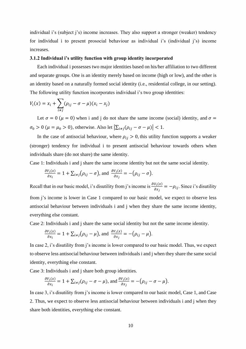
3.1.2 Individual i’s utility function with group identity incorporated

Each individual i possesses two major identities based on his/her affiliation to two different

and separate groups. One is an identity merely based on income (high or low), and the other is

an identity based on a naturally formed social identity (i.e., residential college, in our setting).

The following utility function incorporates individual i’s two group identities:

𝑉𝑖(𝑥) = 𝑥𝑖 + ∑(𝜌𝑖𝑗 − 𝜎 − 𝜇

𝑖≠𝑗

)(𝑥𝑖 − 𝑥𝑗)

Let 𝜎 = 0 (𝜇 = 0) when i and j do not share the same income (social) identity, and 𝜎 =

𝜎0 > 0 (𝜇 = 𝜇0 > 0), otherwise. Also let |∑ (𝜌𝑖𝑗𝑖≠𝑗 − 𝜎 − 𝜇)| < 1.

In the case of antisocial behaviour, where 𝜌𝑖𝑗 > 0, this utility function supports a weaker

(stronger) tendency for individual i to present antisocial behaviour towards others when

individuals share (do not share) the same identity.

Case 1: Individuals i and j share the same income identity but not the same social identity.

𝜕𝑉𝑖(𝑥)

𝜕𝑥𝑖= 1 + ∑ (𝜌𝑖𝑗 − 𝜎)𝑖≠𝑗 , and

𝜕𝑉𝑖(𝑥)

𝜕𝑥𝑗= −(𝜌𝑖𝑗 − 𝜎).

Recall that in our basic model, i’s disutility from j’s income is 𝜕𝑈𝑖(𝑥)

𝜕𝑥𝑗= −𝜌𝑖𝑗. Since i’s disutility

from j’s income is lower in Case 1 compared to our basic model, we expect to observe less

antisocial behaviour between individuals i and j when they share the same income identity,

everything else constant.

Case 2: Individuals i and j share the same social identity but not the same income identity.

𝜕𝑉𝑖(𝑥)

𝜕𝑥𝑖= 1 + ∑ (𝜌𝑖𝑗 − 𝜇)𝑖≠𝑗 , and

𝜕𝑉𝑖(𝑥)

𝜕𝑥𝑗= −(𝜌𝑖𝑗 − 𝜇).

In case 2, i’s disutility from j’s income is lower compared to our basic model. Thus, we expect

to observe less antisocial behaviour between individuals i and j when they share the same social

identity, everything else constant.

Case 3: Individuals i and j share both group identities.

𝜕𝑉𝑖(𝑥)

𝜕𝑥𝑖= 1 + ∑ (𝜌𝑖𝑗 − 𝜎 − 𝜇)𝑖≠𝑗 , and

𝜕𝑉𝑖(𝑥)

𝜕𝑥𝑗= −(𝜌𝑖𝑗 − 𝜎 − 𝜇).

In case 3, i’s disutility from j’s income is lower compared to our basic model, Case 1, and Case

2. Thus, we expect to observe less antisocial behaviour between individuals i and j when they

share both identities, everything else constant.

11

Case 4: Individuals i and j share neither group identity. This case represents our basic model.

3.2 Predictions

Applying this analysis to our three environments, we expect to observe the following

orderings for overall, across income, and within income antisocial behaviour:

Overall: Random > Mixed = Common20

Across: Random = Common > Mixed

Within: Random > Mixed > Common

In our Random environment, subsets of subjects share income identity but there is no shared

social identity. In this setting we expect to observe significant across income identity attacks

since there is no shared identity of either type to mitigate antisocial behaviour and significant

within income identity attacks since there is no observed shared social identity to mitigate

antisocial behaviour. In our Mixed environment, relative to our Random environment, we

expect to observe less across income identity attacks and less within income identity attacks

because in both cases, there is some shared social identity to mitigate antisocial behaviour. In

our Common environment, relative to our Random environment, we expect similar levels of

across income identity attacks considering there is no shared social identity to mitigate

antisocial behaviour and less within income identity attacks since there is shared social identity

to mitigate antisocial behaviour. Finally, in the Common environment, across income antisocial

behaviour should be higher relative to the Mixed environment; in the Mixed there is some

shared social identity to mitigate antisocial behaviour. In contrast, in the Common

environment, relative to the Mixed, we expect less within income antisocial behaviour; in the

Common all subjects share the same social identity, mitigating antisocial behaviour. Whether

our Mixed or our Common environment will exhibit more overall antisocial behaviour will

depend on the relative strength of shared income identity and shared social identity to reduce

antisocial behaviour.

Our analysis suggests the following hypotheses:

Hypothesis 1: Antisocial behaviour is most observed in the Random environment

in which social identity is not revealed.

Hypothesis 2a: We expect more antisocial behaviour within income types in the

Random environment than the Mixed environment and in the Mixed environment

relative to the Common environment.

20 This differs to the predictions of Mogues and Carter (2005).

12

Hypothesis 2b: We also expect antisocial behaviour within income identities to be

targeted based on subjects’ social identity in the Mixed environment.

Hypotheses 2a and 2b are consistent with some stylized facts. For example, there is a long

history in the United States (such as, the “no Irish need apply” signs of the early 19th century)

of inter-social group conflict among members of the same, or similar, income identity. Low

income workers of one social group, fearing competition for jobs, often direct their animosity

towards low income workers of a different social group, newly arrived in the country. A more

recent example is the anti-Mexican, and more broadly anti-immigrant, sentiments prevalent in

the United States today. A 2015 poll found that 51% of respondents believe illegal immigrants

are taking jobs away from U.S. citizens.21 This sentiment was most prevalent among

respondents earning $50,000 or less. Robust empirical evidence on this conjecture is however

scarce due to the difficulty of identifying perpetrators of targeted antisocial behaviour.

Hypothesis 3a: We expect more antisocial behaviour across income types in the

Random and Common environments than in the Mixed environment.

Hypothesis 3b: We also expect antisocial behaviour across income identities to be

targeted based on subjects’ social identities in the Mixed environment.

Hypotheses 3a and 3b are consistent with the literature investigating inequality and conflict.

More conflict may be generated when social identity overlaps with income differences, as in

the case of socially embedded inequality. Also, antisocial behaviour is likely directed at

outgroups (see, for example, Tajfel et al. 1971; Brewer 1979; Mullen et al. 1992). Finally, it

must be noted that, while our predictions apply to both HI and LI types, we believe observed

antisocial behaviour should be more prevalent for LI than HI. It is our expectation that LI types

are most likely to be envious and, as a result, engage in antisocial behaviour. Previous evidence

has shown that, when individuals have different income levels, antisocial behaviour is usually

targeted towards those who are richer or have higher status (Gino and Pierce, 2009a 2009b;

Cikara and Fiske, 2013; Grossman et al., 2016).

21 http://www.newsmax.com/Newsfront/illegal-immigration-rasmussen-poll/2015/08/14/id/670157/

13

4. Results

We start this section by reporting the subject characteristics of our sample. We then

examine aggregate rates of antisocial behaviour and behaviour within and across income

groups.

Subjects’ characteristics are reported in Table 2. Background characteristics by income

identity and their differences are reported in columns 1 – 3, respectively. We do not observe

any statistically significant difference between subjects across income identities. The F-statistic

of overall significance (1.11) cannot reject the null hypothesis that observable characteristics

are similar on average across HI and LI. We also report subjects’ characteristics by

environment (columns 4 – 6) and pairwise differences in columns 7 – 9. We find only minor

differences and the three F-statistic measures (1.12, p-value=0.349; 0.62, p-value=0.851; 1.11,

p-value=0.360) cannot reject the null hypothesis that on average the characteristics are similar

across the three environments. Overall, this suggests that the sample is balanced across

different dimensions.

In the first stage of the experiment, on average, subjects earn 558.3 cents in both the

Random and Common environments and 536.0 cents in the Mixed environment. These

differences in earnings are not statistically significant across environments.22 As expected,

earning differences across income identities are statistically significant (HI subjects averaged

733.01 cents, while LI subjects averaged 369.51 cents, p-value=0.000).

4.1 Aggregate rates of antisocial behaviour

In this section, we begin by investigating attacking behaviour at the aggregate level,

following this we investigate the heterogeneity of attacking behaviour. We start by testing

Hypothesis 1. We expect higher overall rates of antisocial behaviour in the Random

environment, due to higher rates of attacks both within and across income groups in this setting.

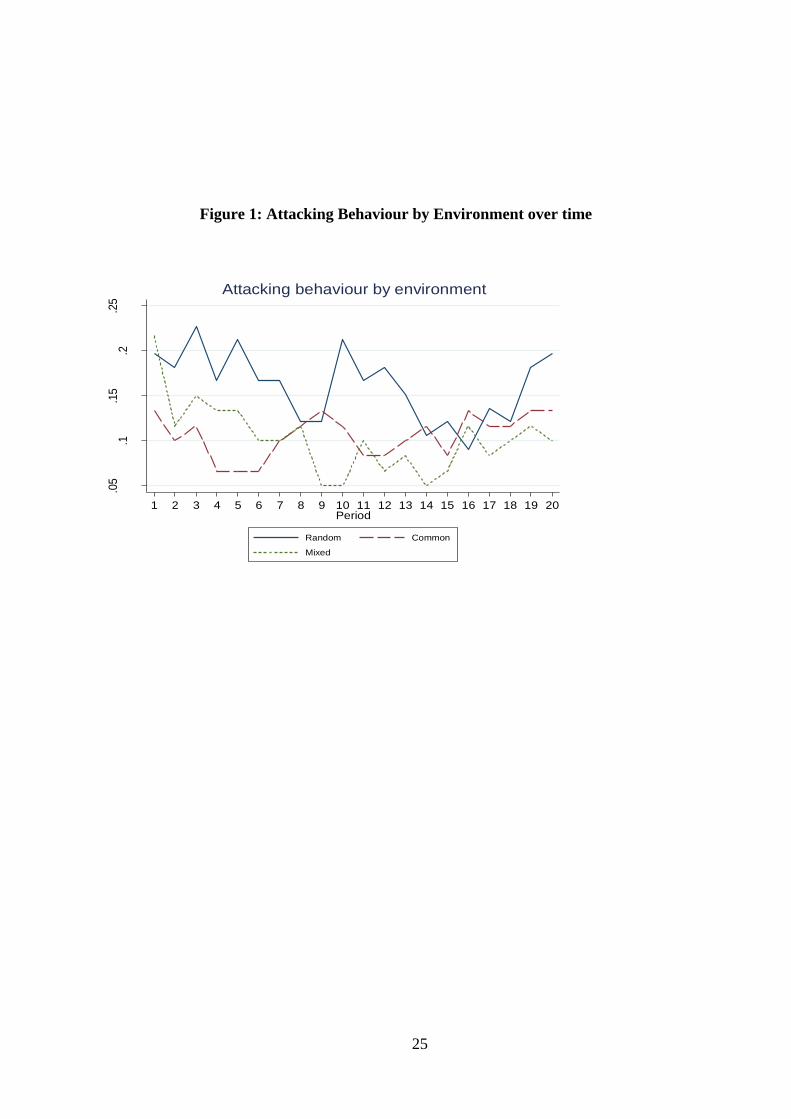
We illustrate attacking behaviour across periods by environment in Figure 1. Attacking

behaviour appears to be quite similar across periods in the Mixed and Common environments

with a generally higher rate of attacking in our Random environment. The aggregate level of

attacking behaviour is reported in Table 3, row 1, columns 1 – 3; columns 4 – 6 report the p-

values for pairwise Wilcoxon rank-sum tests for our three environments. Treating each group

of six as an individual observation, we find that subjects in the Random environment attack

16% of the time relative to 10% in both the Common and Mixed environments with social

identity (p-values=0.094 and 0.089, respectively). As we discuss in more detail below, this

22 Random vs Common, p-value=0.992; Random vs Mixed, p-value=0.584; Common vs Mixed, p-value=0.564.

14

difference is driven by the behaviour of the LI subjects. On the other hand, we find no

difference in the frequency of attacks between the Common and Mixed environments in

aggregate and separately for both HI and LI subjects (all p-values>0.64).

Attacking behaviour may be dependent on many factors including period earnings or

whether one was attacked previously. To control for these factors, we estimate pooled linear

regression. More specifically we estimate equation 1.23

𝑦𝑖𝑗𝑡 = 𝛽0 + 𝛽1𝐿𝐼𝑖𝑗 + 𝛽2𝐶𝑜𝑚𝑚𝑜𝑛𝑖𝑗 + 𝛽3𝑀𝑖𝑥𝑒𝑑𝑖𝑗 + 𝜕1𝑋𝑖𝑗𝑡 + 𝜀𝑖𝑗𝑡 (1)

Our dependent variable is “𝐴𝑡𝑡𝑎𝑐𝑘𝑖𝑗𝑡” (=1 if Subject i attacks subject j in period t, and 0

otherwise). Consistent with our theoretical model, the independent variables are:

“𝐶𝑜𝑚𝑚𝑜𝑛𝑖𝑗” = 1 if the environment is Mixed, and 0 otherwise,

“𝑀𝑖𝑥𝑒𝑑𝑖𝑗” = 1 if the environment is Mixed, and 0 otherwise,

We also include a vector of controls denoted by 𝑋𝑖𝑗𝑡. These include

“𝐷𝑖𝑓𝑓𝑖𝑗𝑡” = the difference between subject j’s earnings and that of subject

i at the beginning of period t,

“𝑆𝑎𝑚𝑒 𝑇𝑦𝑝𝑒𝑖𝑗” = 1 if subject i and j have the same income identity, and 0

otherwise,

“𝑇𝑦𝑝𝑒 𝐿𝐼𝑖𝑗” = 1 if subject i belongs to the LI group

“𝑇𝑎𝑟𝑔𝑒𝑡 𝐴𝑡𝑡𝑎𝑐𝑘𝑖𝑡−1” = 1 if subject i was attacked in the last period,

“Period” = 1,…, 20.

Standard errors are clustered at the group and individual levels. Results are reported in

Table 4. Column 1 reports the model without controls; column 2 includes controls.24 We find

little evidence that aggregate rates of antisocial behaviour differ across our three environments.

Several other factors appear to be related to attacking behaviour, such as a group member’s

income identity and if a subject was attacked in the previous period.

Differences across environments are perhaps difficult to uncover in the aggregate as both

within and across income type behaviour are combined. As shown by the non-parametric

results in Table 3 when we disaggregate behaviour of HI and LI types, significant differences

23 Prior to estimation we set up the data such that each subject had five observations; each observation represents

the interaction with a group member. 24 In all future regressions we include controls, as we believe this to be a more conservative estimate.

15

in antisocial behaviour are observed. To test the impacts of HI and LI by environment we re-

estimate equation 1 but include interaction terms between income type and environments. We

estimate the following equation:

𝑦𝑖𝑗𝑡 = 𝛽0 + 𝛽1𝐿𝐼𝑖𝑗 + 𝛽2𝐶𝑜𝑚𝑚𝑜𝑛𝑖𝑗 + 𝛽3𝑀𝑖𝑥𝑒𝑑𝑖𝑗 + 𝛽4𝑀𝑖𝑥𝑒𝑑 ∗ 𝑇𝑦𝑝𝑒𝐿𝐼𝑖𝑗 +

𝛽5𝐶𝑜𝑚𝑚𝑜𝑛 ∗ 𝑇𝑦𝑝𝑒𝐿𝐼𝑖𝑗 + 𝜕1𝑋𝑖𝑗𝑡 + 𝜀𝑖𝑗𝑡 (2)

Results are reported in Table 4, column 3. Panel B reports comparisons across coefficients, i.e.,

the differential effects. To estimate the differential effects, we calculate the total effect for each

subgroup (e.g., common HI on 𝑦𝑖𝑗𝑡). The differential effect is then the difference between each

subgroup. Consistent with the non-parametric results, we find that attacking behaviour across

treatments is driven by LI subjects. A LI subject in the random treatment attacks at a 2

percentage points higher rate relative to the Common and Mixed environments.

In summary, at the aggregate level, we do not find evidence to support Hypothesis 1.

However, this is not true for LI subjects; for this subsample, results are consistent with

Hypothesis 1. These findings are summarized in the following results.

Result 1a: At the aggregate level we find no significant difference in rates of

antisocial behaviour in environments in whichw income inequality is socially

embedded (Common environment) relative to the Mixed environment.

Result 1b: We find no significant difference in aggregate antisocial behaviour in

environments where social identity is unknown (Random environment) relative to

environments where it is known, irrespective of the composition of social and

income groups. However, when we compare behaviour by income group we find

that LI subjects attack more often when social identity is unknown.

4.2 Antisocial behaviour within income groups

Our aggregate results are silent on the possible heterogeneity within social environments.

Who attacks within these environments and whether this differs across settings may be

important in understanding how the differing inequality environments influence behaviour and

what policies may be effective within each social context.

16

Recall that we expect less antisocial behaviour within income identities (within HI or LI)

in the Common environment compared to the Random and Mixed environments (Hypothesis

2a). First consider within income identity attacks (Table 3, rows 4 and 5). We find no

significant difference in antisocial behaviour within HI subjects across environments. LI

subjects’ antisocial behaviour towards their own income identity is, however, significantly

more frequent in the Random environment than the Common environment (p-value=0.001).25

This is consistent with our prediction: within income identity attacks (at least among LI

subjects) are fewer when subjects are informed that they share a common social identity. The

antisocial behaviour of LI subjects towards their own income identity is also significantly more

frequent in the Random environment than the Mixed environment (p-value=0.055). One

interpretation is that, consistent with online trolling behaviour of anonymous individuals, our

subjects may feel more comfortable targeting socially anonymous targets in the Random

treatment. Another interpretation is that in the Mixed environment, there is only one social

identity outsider within an income type, whereas in the Random, all the subjects within an

income type could hold a different social identity.

To examine the robustness of this result, we again conduct linear regressions with clustered

standard errors at the individual and group levels. Results are reported in Table 5, column 1.

Our regression model follows.

𝑦𝑖𝑗𝑡 = 𝛽0 + 𝛽1𝐿𝐼𝑖𝑗 + 𝛽2𝐶𝑜𝑚𝑚𝑜𝑛𝑖𝑗 + 𝛽3𝑀𝑖𝑥𝑒𝑑𝑖𝑗 + 𝛽4𝐺𝑀 𝐿𝐼𝑖𝑗𝑡 +

𝛽5𝐺𝑀 𝐿𝐼𝑖𝑗𝑡 ∗ 𝐿𝐼𝑖𝑗𝑡 + 𝜕1𝑋𝑖𝑗𝑡 + 𝜀𝑖𝑡 (3)

We introduce 𝛽4 (an indicator variable) if subject j is from the LI group. 𝛽5 represents the

marginal propensity for LI subject i to attack LI group member j. All regression results include

controls, 𝑋𝑖𝑗𝑡. Consistent with the non-parametric results we find that LI subjects are

significantly more inclined to attack someone from their own income group. An LI subject

attacks a LI group member 7.3 percentage points more often.

To understand whether attacking behaviour towards one’s own income group differs across

environments, we estimate the following separately for high (Table 5, column 2) and low

income (Table 5, column 3) subjects:

25 Each group is treated as an independent observation.

17

𝑦𝑖𝑗𝑡 = 𝛽0 + 𝛽1𝐶𝑜𝑚𝑚𝑜𝑛𝑖𝑡 + 𝛽2𝑀𝑖𝑥𝑒𝑑𝑖𝑡 + 𝛽3𝐺𝑀 𝐿𝐼𝑖𝑗𝑡 + 𝛽4𝐺𝑀 𝐿𝐼𝑖𝑗𝑡 ∗

𝐶𝑜𝑚𝑚𝑜𝑛𝑖𝑗𝑡 + 𝛽5𝐺𝑀 𝐿𝐼𝑖𝑗𝑡 ∗ 𝑀𝑖𝑥𝑒𝑑𝑖𝑗𝑡 + 𝜕1𝑋𝑖𝑡 + 𝜀𝑖𝑡 (4)

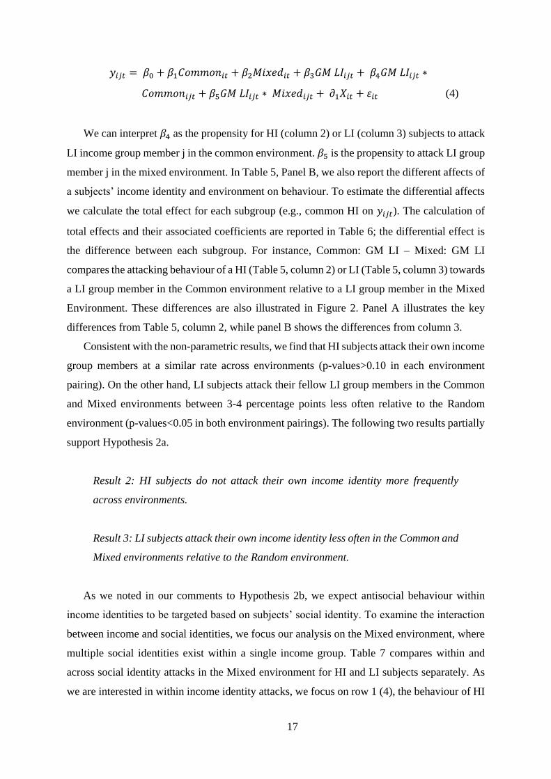
We can interpret 𝛽4 as the propensity for HI (column 2) or LI (column 3) subjects to attack

LI income group member j in the common environment. 𝛽5 is the propensity to attack LI group

member j in the mixed environment. In Table 5, Panel B, we also report the different affects of

a subjects’ income identity and environment on behaviour. To estimate the differential affects

we calculate the total effect for each subgroup (e.g., common HI on 𝑦𝑖𝑗𝑡). The calculation of

total effects and their associated coefficients are reported in Table 6; the differential effect is

the difference between each subgroup. For instance, Common: GM LI – Mixed: GM LI

compares the attacking behaviour of a HI (Table 5, column 2) or LI (Table 5, column 3) towards

a LI group member in the Common environment relative to a LI group member in the Mixed

Environment. These differences are also illustrated in Figure 2. Panel A illustrates the key

differences from Table 5, column 2, while panel B shows the differences from column 3.

Consistent with the non-parametric results, we find that HI subjects attack their own income

group members at a similar rate across environments (p-values>0.10 in each environment

pairing). On the other hand, LI subjects attack their fellow LI group members in the Common

and Mixed environments between 3-4 percentage points less often relative to the Random

environment (p-values<0.05 in both environment pairings). The following two results partially

support Hypothesis 2a.

Result 2: HI subjects do not attack their own income identity more frequently

across environments.

Result 3: LI subjects attack their own income identity less often in the Common and

Mixed environments relative to the Random environment.

As we noted in our comments to Hypothesis 2b, we expect antisocial behaviour within

income identities to be targeted based on subjects’ social identity. To examine the interaction

between income and social identities, we focus our analysis on the Mixed environment, where

multiple social identities exist within a single income group. Table 7 compares within and

across social identity attacks in the Mixed environment for HI and LI subjects separately. As

we are interested in within income identity attacks, we focus on row 1 (4), the behaviour of HI

18

(LI) subjects towards HI (LI) across and within social groups. We find that the frequency of

within social identity attacks among LI subjects is significantly lower than that of across social

identity attacks (0.017 versus 0.09: p-value=0.053). This pattern is also observed among HI

subjects, but the difference is not statistically significant (p-value=0.82).

Results from a linear regression are reported in Table 8. Column 1 reports attacking

behaviour by HI subjects only, column 2 reports attacking behaviour by LI subjects. Again, we

restrict analysis to the Mixed environment. The key variable of interest in column 1 is

𝑊𝑖𝑡ℎ𝑖𝑛 𝑆𝑜𝑐𝑖𝑎𝑙 𝐼𝑑𝑒𝑛𝑡𝑖𝑡𝑦𝑖𝑗 which represents HI subjects’ marginal propensity to attack other

HI group members with the same social identity. In column 2 we are interested in

𝑊𝑖𝑡ℎ𝑖𝑛 𝑆𝑜𝑐𝑖𝑎𝑙 𝐼𝑑𝑒𝑛𝑡𝑖𝑡𝑦𝑖𝑗*𝑆𝑎𝑚𝑒 𝑇𝑦𝑝𝑒𝑖𝑗 which represents the marginal propensity for LI to

attack other LI group members with the same social identity. We find that HI subjects do not

differentiate between social identities when attacking other HI subjects. In contrast, LI subjects

are significantly less inclined to attack another LI group member when they have the same

social identity.26 From this result we can partially accept Hypothesis 2b; only LI subjects attack

based on one’s social identity.

Result 4: In the Mixed environment, LI subjects target other LI subjects less

frequently when they share social identity. However, HI subjects do not change

attacking behaviour based on a group member’s social identity.

4.3 Attacking behaviour across income identities

We next turn to attacking behaviour directed towards one’s outgroup income identity.

Hypothesis 3a suggests that outgroup antisocial behaviour should be lower in the Mixed

environment relative to the Random and Common environments. This is consistent with the

theory of socially embedded income inequality since, in the Mixed setting, social identity

overlaps with income identity and social identity can mitigate across income antisocial

behaviour.

According to Table 3, rows 6 and 7, for HI subjects, the frequency of attacks across income

identities is not significantly different across environments. For LI subjects, the frequency of

attacks across income identities is significantly different between the Mixed environment and

the Random environment (p-value=0.061).

26 We investigate the across income identity attacking behaviour more precisely in the next section.

19

For further analysis, we return to Table 5, columns 2 and 3. We are interested in

understanding whether HI (LI) subjects differentially attack LI (HI) across environments. In

column 2, our key variable of interest is the LI difference estimate reported in Panel B (i.e.,

Common: GM LI – Mixed: GM LI), while in column 3 we are interested in HI differences i.e

Common: GM HI – Random: GM HI. Our results in column 2 indicate that HI subjects attack

LI’s at a similar rate across our three environments (p-values>0.10 for each environment

pairing). On the other hand, LI subjects attack HI subjects less often in the Common than in

the Random environment (p-value=0.041). Table 5 (column 2) also indicates that, consistent

with our theoretical model, antisocial behaviour by HI individual i is most observed towards

subject j, when income inequality (Diffijt) increases in i’s disadvantage. This pattern, although

observed for LI subjects (column 3), is statistically insignificant. These observations are

partially consistent with Hypothesis 3a.

Result 5: There is no evidence that HI subjects attack LI subjects at a significantly

different rate across environments.

Result 6: LI subjects attack subjects at a higher rate in the Random relative to the

Common environment, however there is no difference between the Mixed and the

Random environment.

These results suggest that social identity can partially explain rates of antisocial behaviour

in environments where income inequality exists. Hypothesis 3b tests the impact of social

identity in more detail by comparing across income identity attacks in the Mixed environment.

According to Table 7, row 2, LI subjects attack across social identity HI subjects at a higher

rate than within social identity subjects (p-value=0.040). The same pattern is observed for HI

subjects (row 3) but the difference is statistically insignificant (p-value=0.175).

Returning to Table 8, we are interested in understanding whether HI (LI) subjects attack LI

(HI) subjects who have a common social identity or with the opposing social identity. For this

reason, we are interested in the comparison 𝐺𝑀 𝐿𝐼: 𝑊𝑖𝑡ℎ𝑖𝑛 𝑆𝑜𝑐𝑖𝑎𝑙 𝐼𝑑𝑒𝑛𝑡𝑖𝑡𝑦 −

𝐴𝑐𝑟𝑜𝑠𝑠 𝑆𝑜𝑐𝑖𝑎𝑙 𝐼𝑑𝑒𝑛𝑡𝑖𝑡𝑦 in column 1 (Panel B) and 𝑊𝑖𝑡ℎ𝑖𝑛 𝑆𝑜𝑐𝑖𝑎𝑙 𝐼𝑑𝑒𝑛𝑡𝑖𝑡𝑦𝑖𝑗 in column 2

(Panel A). We find little evidence that either HI or LI subjects attack across income identity

members more frequently if they are part of their own or their opposing social group. We thus

do not find support for Hypothesis 3b.

20

Result 7: In the Mixed environment, we find little evidence that subjects attack

members of their social group who are of a different income identity more often

than those with both different social and income identities.

In summary, our results show that consistent with theoretical intuition, the larger the

income difference between individuals, the higher the probability of antisocial behaviour. The

two group identities interestingly appear to have opposing effects on antisocial behaviour, with

individuals more likely to attack those with similar income identity and less likely to attack

those with the same social identity. The findings from the experiment are consistent with the

hypotheses for the LI subjects. Most of the antisocial behaviour is instigated by LI subjects;

they target other LI subjects more than HI subjects and are significantly influenced by social

identity. In environments in which social identity is made explicit, LI direct their antisocial

behaviour away from LI members of their own social group and towards LI members outside

their social group. 27

5. Discussion

Individuals do not make decisions in a vacuum; they are influenced by groups within

society. Despite a large body of experimental research studying inequality and the behaviour

of high and low income individuals, there is little research studying the interaction between

social identity and income identity. Social identity, such as one’s ethnicity, can have important

consequences for the effective functioning of modern societies. When social identity overlaps

with income identity (a term called socially embedded inequality), groups have another

dimension in which to unify, potentially increasing antisocial behaviour. In this paper, we

examine how varying the composition of income and social identities impacts antisocial

behaviour.

Using a unique experiment and sample, we find little evidence that antisocial behaviour

differs between an environment with socially embedded inequality relative to an environment

in which social identity and income groups are mixed. This is, to our knowledge, the first

empirical examination of the concept of socially embedded inequality and the news is

27 Using data from stage 3, we also examine the relationship between past antisocial behaviour and cooperation.

We find that subjects who exhibited antisocial tendencies in stage 2 continue their antisocial behaviour by

cooperating less in the public goods game irrespective of the social environment they originated from. As

cooperation is not the main focus of the paper we do not investigate this further. Summary results reported in

Table A1 and Table A2.

21

promising. We show that environments with social identity including one that represents

socially embedded inequality display significantly lower rates of antisocial behaviour relative

to settings without social identity, especially for low income subjects. This suggests that it is

not the combination of income inequality and social identity that matter per se, but social

identity itself. Upon the introduction of a social identity, low income subjects are less likely to

attack someone from their own income group. On the other hand, we find that high income

people do not change their behaviour, indicating that social identity impacts the behaviour of

low income persons differently to those with high income.

Our results suggest that a shared social identity can mitigate antisocial behaviour among

the lower income class. While this may be a relatively optimistic result, changes occurring in

society that may weaken feelings of a common social identity raise concerns. The driving force

behind many of these changes has been the increasing concentration of wealth in society.

Picketty (2014) argues that wealth over the past 40 years has become increasingly concentrated

in the hands of the richest families. Emmons and Ricketts (2015) find that this trend is

increasing. For example, this increasing concentration of wealth has resulted in the shrinking

of the middle class in the United States and increased income polarization.28 A possible by-

product of this income concentration is increasing segregation of housing by income.29 Another

possible by-product has been the increasing segregation of higher education by income. A

recent study reports that there were more students drawn from families in the top 1% of the

income distribution enrolled at the elite universities than from families from the bottom half of

the income distribution (Chetty et al., 2017).30 These changes suggest a possible weakening in

a common social identity, which our research suggests could lead to higher rates of antisocial

behaviour.

28 https://blogs.imf.org/2016/06/28/rising-income-polarization-in-the-united-states/ 29 In the first decade of the 21st century, the number of units in gated communities rose by more than 50% and by

2012, approximately 10% of all occupied homes are now in gated communities (Benjamin 2012). Gated

communities are private residential settlements protected from outsiders by guarded gates, walls, and fences and

they provide many of the public services provided by local municipalities. The rise of gated communities has

occurred at the same time that local government spending on public services has declined (Frantz 2000). 30 The researchers also find that, relative to the 1980 birth cohort, the fraction of students from the 1991 birth

cohort from bottom-quintile families enrolled at colleges with high rates of bottom-to-top-quintile mobility fell

sharply.

22

References

Abbink, K. and B. Herrmann. 2011. The moral costs of nastiness. Economic Inquiry, 49: 631-

33.

Abbink, K. and A. Sadrieh. 2009. The pleasure of being nasty. Economic Letters, 105:306-08.

Albert, M. and V. Mertins. 2008. Participation and decision making: A three-person power-to-

take experiment. Justus-Liebig-University Giessen Discussion Paper Series in Economics.

Alesina, A. and R. Perotti. 1996. Income distribution, political instability, and investment.

European Economic Review, 40: 1203–1228.

Beckman S.R., J.P. Formby, W.J. Smith, and B. Zheng. 2002. Envy, malice, and pareto

efficiency: An experimental examination. Social Choice and Welfare, 19: 349-367.

Benjamin, R. 2012. The gated community mentality. New York Times, March 29, 2012.

Bosman, R. and F. van Winden. 2002. Emotional hazard in a power-to-take experiment. The

Economic Journal, 112: 147–169

Bosman, R., H. Hennig-Schmidt and F. van Winden. 2006. Exploring group decision making

in a power-to-take experiment, Experimental Economics, 9: 35 – 51.

Brewer, M.B. 1979. In-group bias in the minimal intergroup situation: A cognitive-motivational

analysis. Psychological Bulletin, 86: 307-324.

Buckley, E. and R. Croson. 2006. Income and wealth heterogeneity in the voluntary provision of

linear public goods. Journal of Public Economic, 90: 935–955

Cason, T. and Mui, V. L. 2002a. Fairness and sharing in innovation games: a laboratory

investigation. Journal of Economic Behavior and Organization, 48: 243–264.

Cason T.N., T. Saijo, and T. Yamato. 2002b. Voluntary participation and spite in public good

provision experiments: An international comparison. Experimental Economics, 5: 133-

153.

Chen, Y. and S.X. Li. 2009. Group identity and social preferences. American Economic

Review, 99: 431-457.

Chetty, R., J.N. Friedman, E. Saez, N. Turner, and D. Yagan. 2017. Mobility report cards:

The role of colleges in intergenerational mobility. The Equality of Opportunity

Project.

Cikara, M. and S.T. Fiske. 2013. Their pain, our pleasure: stereotype content and

schadenfreude. Annals of the New York Academy of Sciences, 1299: 52-59

Duclos, J.-Y., Esteban, J. and Ray, D. 2004. Polarization: Concepts, measurement and

estimation. Econometrica, 72: 1737-1772.

23

Emmons, W.R. and L.R. Ricketts. 2015. The importance of wealth is growing. In the Balance,

issue 15. Federal Reserve Bank of St. Louis.

Esteban, J.M. and D. Ray. 1994. On the measurement of polarization. Econometrica, 62: 819-851.

Figueroa, A., T. Altamirano, and D. Sulmont. 1996, Social Exclusion and Inequality in Peru,

International Labor Organisation. Geneva.

Fischbacher, U. 2007. z-Tree: Zurich toolbox for ready-made economic experiments.

Experimental Economics, 10: 171-178.

Frantz, K., 2000. Gated Communities in the USA – A new trend in Urban Development.

Espace, populations, sociétés, 18: 101-113.

Gino, F. And L. Pierce. 2009a. Dishonesty in the name of equity. Psychological Science, 20:

1153-1160.

Gino, F. and L. Pierce. 2009b. The abundance effect: Unethical behavior in the presence of

wealth. Organizational Behavior and Human Decision Processes, 109: 142-155.

Goette, L., D. Huffman, and S. Meier. 2006. The Impact of Group Membership on Cooperation

and Norm Enforcement: Evidence Using Random Assignment to Real Social Groups.

American Economic Review, 96: 212-216.

Grossman, P.J., and M. Komai, 2016. Antisocial behavior in hierarchal groups, Monash

Economics Working Papers 02-13, Monash University, Department of Economics.

Gurr, T.R. 1993. Minorities at Risk: A Global View of Ethnopolitical Conflicts, Institute of

Peace Press: Washington DC.

Lane, T. 2016. Discrimination in the laboratory: A meta-analysis of economics experiments.

European Economic Review, 90: 375-402

Mogues, T. and M.R. Carter. 2005. Social capital and the reproduction of inequality in

polarized societies. Journal of Economic Inequality, 3: 193–219.

Mullen, B., R. Brown, and C. Smith. 1992. Ingroup bias as a function of salience, relevance,

and status: An integration. European Journal of Social Psychology, 22: 103–122.

Piketty, T. 2014. Capital in the Twenty-First Century. Cambridge, Mass., and London: The

Belknap Press of Harvard University Press.

Robinson, J.A. 2001. Social Identity, Inequality and Conflict. Economics of Governance, 2:

85-99.

Saijo, T. and H. Nakamura. 1995. The “spite” dilemma in voluntary contribution mechanism

experiments. Journal of Conflict Resolution, 39: 535-560.

Sen, A. 1973. On Economic Inequality. Oxford: Clarendon Press.

24

Stewart, F. 2001. Horizontal inequalities: A neglected dimension of development. United

Nations University, World Institute for Development Economics Research.

Tajfel, H. 1978. Interindividual behavior and intergroup behavior. In: H. Tajfel (Ed.).

Differentiation between Social Groups. London: Academic Press, pp. 27-60.

van Dijk, F., J. Sonnemans, F. van Winden. 2002. Social ties in a public good experiment.

Journal of Public Economics, 85: 275–299.

Weng, Q. and F. Carlsson. 2015. Cooperation in teams: The role of identity, punishment, and

endowment distribution. Journal of Public Economics, 126: 25-38.

Zizzo, D.J. 2003. Money burning and rank egalitarianism with random dictators. Economic

Letters, 81: 263-266.

Zizzo, D.J. and A.J. Oswald. 2001. Are people willing to pay to reduce others’ incomes?

Annales d’ Economie et de Statistique, 63: 39-65.

25

Figure 1: Attacking Behaviour by Environment over time

.05

.1.1

5.2

.25

Pro

b. o

f atta

ckin

g

1 2 3 4 5 6 7 8 9 10 11 12 13 14 15 16 17 18 19 20Period

Random Common

Mixed

Attacking behaviour by environment

26

Figure 2: Aggregate atacking behaviour by environment over time

Note: Panel A illustrates the key differences shown in Table 5, panel B, column 2. Analysis is restricted

to HI subjects only. Panel B illustrates differences shown in Table 5, panel B, column 3. Analysis is restricted to

LI subjects only. Com refers to the common treatment, Mix to the Mixed treatment and Ran to the Random

treatment. Confidence intervals at the 90% level.

27

Table 1: Environment Overview

Environments

Random Common Mixed

Information on Income identity? Yes Yes Yes

Information on Social (College) identity? No Yes Yes

Income identity same for all social groups? N.A. Yes No

28

Table 2: Individual Characteristics

(1) (2) (3) (4) (5) (6) (7) (8) (9)

Variables HI

LI

Diff.

Random

Common

Mixed

Diff.

(4-5)

Diff

(4-6)

Diff

(5-6)

Male 0.47

(0.05)

0.46

(0.05)

0.011

(0.07)

0.439

(0.062)

0.450

(0.065)

0.517

(0.065)

0.011

(0.044)

0.077

(0.090)

-.066

(.092)

Age 19.59

(0.20)

19.46

(0.14)

0.130

(0.24)

19.68

(0.232)

19.38

(0.215)

19.5

(0.174)

0.298

(0.318)

0.182

(0.294)

-0.116

(0.277)

Degree

Economics 0.140

(0.036)

0.086

(0.029)

0.054

(0.046)

0.121

(0.041)

0.050

(0.028)

0.167

(0.049)

0.071

(0.051)

0.045

(0.063)

0.117**

(0.056)

Other Business 0.011

(0.011)

0.00

(0.00)

0.011

(0.011)

0.00

(0.00)

0.017

(0.017)

0.00

(0.00)

0.017

(0.016)

0.00

(0.00)

0.017

(0.017)

Psychology 0.086

(0.029)

0.118

(0.034)

0.032

(0.045)

0.136

(0.043)

0.067

(0.032)

0.100

(0.040)

0.070

(0.054)

0.036

(0.058)

0.033

(0.051)

Sciences 0.473

(0.052)

0.430

(0.052)

0.043

(0.073)

0.454

(0.062)

0.483

(0.065)

0.417

(0.064)

0.029

(0.090)

0.038

(0.089)

0.067

(0.091)

Other 0.290

(0.047)

0.366

(0.050)

0.075

(0.069)

0.288

(0.056)

0.383

(0.063)

0.317

(0.061)

0.095

(0.084)

0.029

(0.082)

0.067

(0.088)

Current Study Year

Freshman 0.398

(0.051)

0.419

(0.051)

0.022

(0.072)

0.424

(0.061)

0.400

(0.064)

0.400

(0.064)

0.024

(0.088)

0.024

(0.088)

0.00

(0.090)

Sophomore 0.345

(0.050)

0.226

(0.044)

0.118*

(0.066)

0.242

(0.053)

0.383

(0.063)

0.233

(0.055)

0.141*

(0.082)

0.009

(0.077)

0.150*

(0.084)

Junior 0.097

(0.031)

0.194

(0.041)

0.097*

(0.051)

0.121

(0.041)

0.133

(0.044)

0.183

(0.050)

0.012

(0.060)

0.062

(0.064)

0.050

(0.067)

Senior 0.151

(0.161)

0.161

(0.038)

0.011

(0.054)

0.212

(0.051)

0.067

(0.032)

0.183

(0.050)

0.145**

(0.062)

0.029

(0.072)

0.117*

(0.060)

Graduate 0.011

(0.011)

0.00

(0.00)

0.011

(0.011)

0.00

(0.00)

0.017

(0.017)

0.00

(0.00)

0.017

(0.008)

0.00

(0.00)

0.017

(0.017)

Religion

Christian 0.452

(0.052)

0.462

(0.052)

0.011

(0.073)

0.515

(0.062)

0.367

(0.063)

0.483

(0.065)

0.148*

(0.088)

0.032

(0.090)

0.117

(0.090)

Buddhist 0.022

(0.015)

0.00

(0.00)

0.022

(0.015)

0.015

(0.015)

0.016

(0.016)

0.00

(0.00)

0.002

(0.022)

0.015

(0.016)

0.017

(0.017)

Muslim 0.054 0.022 0.032 0.030 0.033 0.05 0.003 0.020 0.017

29

(0.024) (0.015) (0.028) (0.021) (0.023) (0.028) (0.032) (0.035) (0.037)

Hindu 0.054

(0.024)

0.054

(0.024)

0.00

(0.033)

0.031

(0.021)

0.083

(0.036)

0.05

(0.028)

0.053

(0.041)

0.020

(0.035)

0.033

(0.046)

Jewish 0.00

(0.00)

0.011

(0.011)

0.011

(0.011)

0.015

(0.015)

0.00

(0.00)

0.00

(0.00)

0.015

(0.016)

0.015

(0.016)

0.00

(0.00)

Other 0.054

(0.024)

0.065

(0.026)

0.011

(0.035)

0.045

(0.026)

0.050

(0.028)

0.083

(0.036)

0.004

(0.038)

0.038

(0.044)

0.033

(0.046)

None 0.366

(0.050)

0.387

(0.051)

0.022

(0.071)

0.348

(0.059)

0.450

(0.067)

0.333

(0.061)

0.102

(0.087)

0.151

(0.085)

0.117

(0.089)

Employed either F/T or P/T 0.280

(0.047)

0.344

(0.049)

0.065

(0.068)

0.334

(0.058)

0.350

(0.062)

0.750

(0.056)

0.017

(0.085)

0.083

(0.082)

0.100

(0.084)

United States Citizen 0.850

(0.037)

0.817

(0.041)

0.032

(0.055)

0.864

(0.043)

0.817

(0.050)

0.183

(0.050)

0.047

(0.066)

0.047

(0.066)

0.00

(0.071)

F-Stat 1.11 1.12 0.62 1.11

Observations 93 93 66 60 60

Note: This table shows the ex post balance in the characteristics of participants in the experiments. Column 3 reports the mean difference in demographic characteristics

between HI and LI subjects. Column 7-9 reports the mean difference in demographic characteristics between participants in the Random and Common environment, Random

and Mixed environment and Common and Mixed respectively. Standard errors in parentheses. *** p < 0.01; ** p < 0.05; * p< 0.10.

30

Table 3: Attacking Behaviour by Environment

Environments Wilcoxon Rank-Sum Test P-values

Row

No.

Random

(1)

Mixed

(2)

Common

(3)

Random v.

Common

(4)

Mixed v.

Common

(5)

Random v.

Mixed

(6)

Overall Attacks

All Subjects Attacking

1 0.161 0.103 0.106 0.094* 0.969 0.089*

HI Subjects Attacking

2 0.102 0.095 0.095 0.942 0.641 0.886

LI Subjects Attacking

3 0.221 0.11 0.117 0.034** 0.938 0.024**

Within Income Type Attacks

HI Subjects Attacking HI subjects

4 0.092 0.078 0.075 0.999 0.845 0.941

LI Subjects Attacking LI subjects

5 0.164 0.087 0.067 0.001*** 0.287 0.055*

Across Income Type Attacks

HI Subjects Attacking LI subjects

6 0.009 0.017 0.02 0.850 0.766 0.791

LI Subjects Attacking HI subjects

7 0.058 0.023 0.05 0.143 0.454 0.061*

Notes: Wilcoxon rank-sum tests are applied to group level data. *** p<0.01, ** p<0.05, * p<0.1.

31

Table 4: Attacking Behaviour Across Environments

(1) (2) (3)

Attack

Player

Attack

Player

Attack

Player

Panel A

𝐷𝑖𝑓𝑓𝑖𝑗𝑡 0.005* 0.002 0.002

(0.003) (0.004) (0.004)

𝐶𝑜𝑚𝑚𝑜𝑛 -0.010 -0.010 -0.001

(0.009) (0.009) (0.013)

𝑀𝑖𝑥𝑒𝑑 -0.011 -0.010 -0.001

(0.008) (0.008) (0.010)

𝑆𝑎𝑚𝑒 𝑇𝑦𝑝𝑒𝑖𝑗 0.037*** 0.037***

(0.007) (0.007)

𝑇𝑦𝑝𝑒 𝐿𝐼𝑖𝑡 0.010 0.021*

(0.008) (0.012)

𝑇𝑎𝑟𝑔𝑒𝑡 𝐴𝑡𝑡𝑎𝑐𝑘𝑖𝑡−1 0.011* 0.011*

(0.006) (0.006)

𝑃𝑒𝑟𝑖𝑜𝑑 -0.000* -0.000* -0.000*

(0.000) (0.000) (0.000)

Common * Type LI -0.018

(0.017)

Mixed * Type LI -0.019

(0.015)

Constant 0.035*** 0.023*** 0.023**

(0.006) (0.006) (0.009)

Panel B: Difference Estimates

𝐶𝑜𝑚𝑚𝑜𝑛 𝐿𝐼 − 𝑅𝑎𝑛𝑑𝑜𝑚: 𝐿𝐼+ -0.021*

(0.012)

𝑀𝑖𝑥𝑒𝑑: 𝐿𝐼 − 𝑅𝑎𝑛𝑑𝑜𝑚: 𝐿𝐼 -0.020*

(0.011)

𝐶𝑜𝑚𝑚𝑜𝑛: 𝐿𝐼 − 𝑀𝑖𝑥𝑒𝑑: 𝐿𝐼 0.001

(0.012)

𝐶𝑜𝑚𝑚𝑜𝑛: 𝐻𝐼 − 𝑅𝑎𝑛𝑑𝑜𝑚: 𝐻𝐼 -0.001

(0.013)

𝑀𝑖𝑥𝑒𝑑: 𝐻𝐼 − 𝑅𝑎𝑛𝑑𝑜𝑚: 𝐻𝐼 -0.001

(0.010)

𝐶𝑜𝑚𝑚𝑜𝑛: 𝐻𝐼 − 𝑀𝑖𝑥𝑒𝑑: 𝐻𝐼 -0.000

(0.011) 18,600 18,600 18,600

R-squared 0.002 0.016 0.003 Notes: This regression includes the full sample, 5 observations exist for each individual, one for each group

member. Standard errors in parentheses clustered at the group and individual level. *** p<0.01, ** p<0.05, *

p<0.1

32

Table 5: Differential Rates of Attacking Behaviour by Environment

Type HI's

only

Type LI's

only (1) (2) (3)

Panel A Attack Player Attack Player Attack Player

𝐷𝑖𝑓𝑓𝑖𝑗𝑡 0.006** 0.008** 0.002 (0.002) (0.003) (0.003)

𝐶𝑜𝑚𝑚𝑜𝑛 -0.010 -0.024 -0.009** (0.009) (0.022) (0.004)

𝑀𝑖𝑥𝑒𝑑 -0.010 -0.005 -0.004 (0.008) (0.025) (0.006)

𝐺𝑀 𝐿𝐼 -0.026*** -0.041** 0.066*** (0.009) (0.018) (0.019)

𝑇𝑦𝑝𝑒 𝐿𝐼𝑖𝑡 -0.027***

(0.010)

𝐺𝑀 𝐿𝐼 ∗ 𝐿𝐼 0.073***

(0.015)

𝑇𝑎𝑟𝑔𝑒𝑡 𝐴𝑡𝑡𝑎𝑐𝑘𝑖𝑡−1 0.010 0.013 0.006 (0.007) (0.008) (0.010)

𝑃𝑒𝑟𝑖𝑜𝑑 -0.000* -0.000 -0.000 (0.000) (0.000) (0.000)

𝑀𝑖𝑥𝑒𝑑 ∗ 𝐺𝑀 𝐿𝐼 0.008 -0.039 (0.024) (0.026)

𝑀𝑖𝑥𝑒𝑑 ∗ 𝐺𝑀 𝐿𝐼 0.040* -0.024 (0.023) (0.029)

Panel B: Difference Estimates

𝐶𝑜𝑚𝑚𝑜𝑛: 𝐺𝑀 𝐿𝐼 − 𝑀𝑖𝑥𝑒𝑑: 𝐺𝑀 𝐿𝐼+ 0.013 0.01 (0.012) (0.029)

𝐶𝑜𝑚𝑚𝑜𝑛: 𝐺𝑀 𝐿𝐼 − 𝑅𝑎𝑛𝑑𝑜𝑚: 𝐺𝑀 𝐿𝐼 0.016 -0.033** (0.012) (0.015)

𝑀𝑖𝑥𝑒𝑑: 𝐺𝑀 𝐿𝐼 − 𝑅𝑎𝑛𝑑𝑜𝑚: 𝐺𝑀 𝐿𝐼 0.003 -0.044** (0.003) (0.017)

𝐶𝑜𝑚𝑚𝑜𝑛: 𝐺𝑀 𝐻𝐼 − 𝑀𝑖𝑥𝑒𝑑: 𝐺𝑀 𝐻𝐼 -0.019 -0.005 (0.019) (0.005)

𝐶𝑜𝑚𝑚𝑜𝑛: 𝐺𝑀 𝐻𝐼 − 𝑅𝑎𝑛𝑑𝑜𝑚: 𝐺𝑀 𝐻𝐼 -0.024 -0.009** (0.022) (0.003)

𝑀𝑖𝑥𝑒𝑑: 𝐺𝑀 𝐻𝐼 − 𝑅𝑎𝑛𝑑𝑜𝑚: 𝐺𝑀 𝐻𝐼 -0.005 -0.004 (0.025) (0.006)

Constant 0.045*** 0.048** 0.017*** (0.012) (0.020) (0.005)

Observations 18,600 9,300 9,300

R-squared 0.017 0.016 0.023

Note: Panel A, Column 1 includes the estimates for the full sample. Column 2 (3) restricts the sample to HI (LI)

subjects. For each regression, five observations exist for each individual, one for each group member. GM refers

to group member. Panel B uses post-estimation linear combination tests of hypotheses using t-tests. Standard

errors in parentheses clustered at the group and individual level. *** p<0.01, ** p<0.05, * p<0.1.

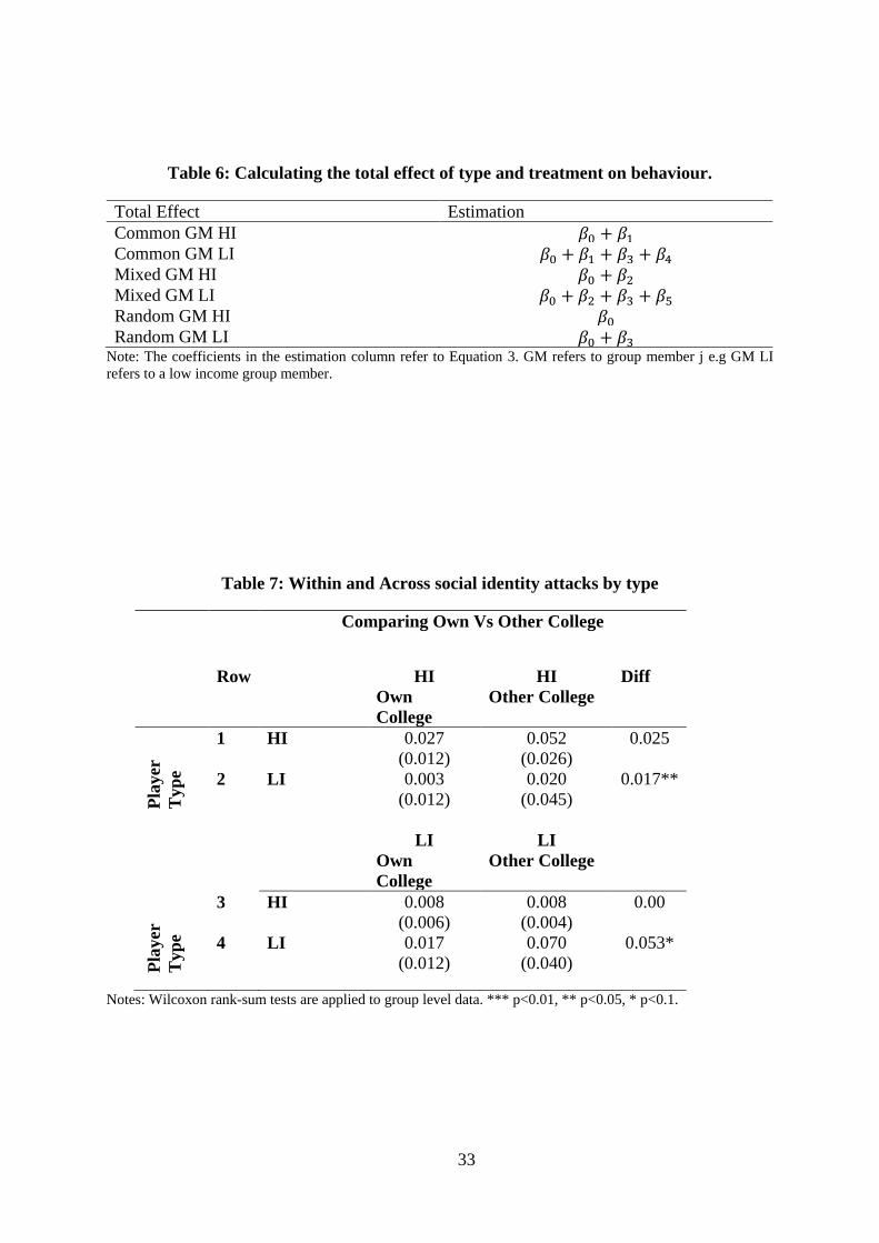
33

Table 6: Calculating the total effect of type and treatment on behaviour.

Total Effect Estimation

Common GM HI 𝛽0 + 𝛽1

Common GM LI 𝛽0 + 𝛽1 + 𝛽3 + 𝛽4

Mixed GM HI 𝛽0 + 𝛽2

Mixed GM LI 𝛽0 + 𝛽2 + 𝛽3 + 𝛽5

Random GM HI 𝛽0

Random GM LI 𝛽0 + 𝛽3 Note: The coefficients in the estimation column refer to Equation 3. GM refers to group member j e.g GM LI

refers to a low income group member.

Table 7: Within and Across social identity attacks by type

Comparing Own Vs Other College

Row HI

Own

College

HI

Other College

Diff

Pla

yer

Typ

e

1 HI 0.027

(0.012)

0.052

(0.026)

0.025

2 LI 0.003

(0.012)

0.020

(0.045)

0.017**

LI

Own

College

LI

Other College

Pla

yer

Typ

e

3 HI 0.008

(0.006)

0.008

(0.004)

0.00

4 LI 0.017

(0.012)

0.070

(0.040)

0.053*

Notes: Wilcoxon rank-sum tests are applied to group level data. *** p<0.01, ** p<0.05, * p<0.1.

34

Table 8: Attacking Behaviour in the Mixed Environment

(1) (2)

HI Only LI Only

Panel A

Attack

Player

Attack

Player

𝐷𝑖𝑓𝑓𝑖𝑗𝑡 0.007** 0.002

(0.003) (0.003)

𝑊𝑖𝑡ℎ𝑖𝑛 𝑆𝑜𝑐𝑖𝑎𝑙 𝐼𝑑𝑒𝑛𝑡𝑖𝑡𝑦𝑖𝑗 -0.017 0.003

(0.015) (0.006)

𝐺𝑀 𝐿𝐼𝑖𝑗 -0.033** 0.065***

(0.015) (0.015)

𝑊𝑖𝑡ℎ𝑖𝑛 𝑆𝑜𝑐𝑖𝑎𝑙 𝐼𝑑𝑒𝑛𝑡𝑖𝑡𝑦𝑖𝑗*𝐺𝑀 𝐿𝐼 0.014 -0.049**

(0.016) (0.019)

𝐴𝑡𝑡𝑎𝑐𝑘𝑖𝑡−1 0.013* 0.006

(0.008) (0.010)

𝑃𝑒𝑟𝑖𝑜𝑑 -0.000 -0.000

(0.000) (0.000)

Panel B: Difference Estimates

𝐺𝑀 𝐿𝐼𝑖𝑗:

𝑊𝑖𝑡ℎ𝑖𝑛 𝑆𝑜𝑐𝑖𝑎𝑙 𝐼𝑑𝑒𝑛𝑡𝑖𝑡𝑦 − -0.003 -0.046**

𝐴𝑐𝑟𝑜𝑠𝑠 𝑆𝑜𝑐𝑖𝑎𝑙 𝐼𝑑𝑒𝑛𝑡𝑖𝑡𝑦𝑖𝑗 (0.005) (0.019)

Constant 0.047*** 0.012***

(0.015) (0.004)

Observations 9,300 9,300

R-squared 0.014 0.025 Note: Panel A Column 1 (3) restricts the sample to HI (LI) subjects. For each regression, 5 observations exist for

each individual, 1 for each group member. GM refers to group member. Panel B uses post-estimation linear

combination tests of hypotheses using t-tests. Standard errors in parentheses clustered at the group and individual

level. *** p<0.01, ** p<0.05, * p<0.1

35

Appendix:

Figure A1: Attacking Behaviour by Environment and Type over Time.

Note: Panel A illustrates attacking behaviour by HI subjects over time by environment, panel B reports behaviour

by LI subjects over time and by environment.

Table A1: Comparison of Group Contribution by Treatment (stage 3)

All (1) (2) (3) (4) (5) (6)

Random Common Mixed

Diff.

(1-2)

Diff.

(1-3)

Diff.

(2-3)

All Group Contribution

3.007

(0.251)

3.38

(0.263)

3.015

(0.269)

0.376

(0.363)

0.007

(0.368)

0.368

(0.376)

LI Group Contributions

3.27

(0.351)

3.26

(0.383)

3.57

(0.335)

0.00

(0.518)

0.294

(0.487)

0.30

(0.508)

HI Group Contributions

2.74

(0.358)

3.50

(0.365)

2.55

(0.538)

0.758

(0.512)

0.279

(0.538)

1.037*

(0.544)

Difference between LI

and HI

-0.530

(0.501)

0.233

(0.529)

-1.10**

(0.524) Note: The table reports the contributions to the public good across all treatments. Column 4 reports mean

differences between column 1 and 2, column 5 reports differences between column 1 and 3 and column 6 reports

differences between column 2 and 3. Differences calculated using a Wilcoxon Rank Sum test. Standard errors

reported in brackets. *** p < 0.01; ** p < 0.05; * p< 0.10.

36

Table A2: Behaviour in the Public Goods Task.

(1) (2) (3) (4) (5) (6)

Contributions Contributions Contributions Contributions Contributions Contributions

HI -0.530 -0.581** 0.757 -0.593* 0.794

(0.502) (0.291) (0.491) (0.309) (0.515)

Common 0.376 -0.006 0.261 -0.196 0.258 -0.214

(0.363) (0.519) (0.354) (0.493) (0.355) (0.491)

Mixed 0.007 0.294 -0.106 0.077 -0.107 0.068

(0.368) (0.485) (0.365) (0.493) (0.367) (0.498)

Common* HI 0.764 0.916 0.939

(0.729) (0.711) (0.714)

Mixed * HI -0.573 -0.367 -0.356

(0.725) (0.727) (0.734)

Proportion target LI -1.972* -2.113**

(1.063) (1.008)

Proportion target HI -1.784** -1.727*

(0.875) (0.929)

Proportion of periods subject attacked -1.876*** -1.914***

(0.657) (0.650)

Proportion of periods subject -0.594 -0.441 -0.594 -0.449

was target of attack (0.751) (0.706) (0.753) (0.707)

Constant 3.008** 2.742** 3.090 2.990 2.845 2.974***

(0.222) (0.240) (0.327) (0.387) (0.582) (0.621)

Observations 186 186 186 186 186 186

R-squared 0.007 0.038 0.070 0.087 0.079 0.098

Note: The dependent variable is the subject’s contribution towards the group account. Each subject is treated as an individual observation. Robust standard errors in parentheses.

*** p<0.01, ** p<0.05, * p<0.1