Impact of RTIASI fast radiative transfer model error on ... · This study quantiﬁes the impact of...

Forecasting Research

Technical Report No. 319

Impact of RTIASI fast radiative transfer modelerror on IASI retrieval accuracy

Vanessa Sherlock

February 21, 2001

The Met. OfficeNWP Division

Room 344London Road

BracknellRG12 2SZ

United Kingdom

c�

Crown Copyright 2000

Permission to quote this paper should be obtained from the above Met. Office division

Please notify us if you change your address or no longer wish to receive these publications.

Tel: 44 (0)1344 856245 Fax: 44 (0)1344 854026 email: [email protected]

Abstract

This study quantifies the impact of specific forward model and Jacobian error characteristics on retrieval accuracy forRTIASI, a fast radiative transfer operator for IASI. In light of previous studies, improved estimates of forward model errorcovariance and fast model Jacobian errors have been made for two versions of RTIASI using three-case and single-case watervapour predictor schemes. Forward model errors present strong correlations within spectral bands and within the windowregions. Error characteristics are comparable for the two versions with the exception of the H � O � � band where the errors forthe single predictor scheme are larger, and error correlation structures differ. The impact of simplifying assumptions to thestructure of the forward model error covariance on retrieval accuracy has been evaluated for two instrumental noise scenariosin two atmospheric sounding scenarios (tropical and sub-arctic atmospheres). In the H � O � � band instrumental noise andforward model error are comparable in magnitude and forward model errors govern long-range correlation structure. In thiscase, neglecting correlation structure can degrade retrieval of upper tropospheric temperature and humidity. In other spectralintervals instrumental noise makes the dominant contribution to the observation error covariance and the error incurred bya diagonal approximation to the forward model error covariance is small. In all cases a block diagonal approximation tothe forward model error covariance matrix accurately captures all relevant correlation features of the full matrix. Errorsin temperature Jacobians have a negligible impact on retrieval accuracy and suggest a target accuracy of 5

�for fast model

Jacobian calculations. Errors in water vapour Jacobians can degrade the accuracy of both temperature and humidity retrievalssignificantly. This is particular issue for the three-case water vapour predictor scheme in the tropical atmosphere. All resultshighlight the sensitivity of retrievals to forward model error characteristics in the H � O � � band. If they can be generalised toa wide range of atmospheric states, a single water vapour predictor scheme is to be preferred, although further improvementsin model performance in the H � O � � band are desirable even in this case.

1 Introduction

In a previous study[1] referred to hereinafter as VS2000, fast radiative transfer model errors were estimated for two IASI fastmodels, RTIASI and PFAAST. It was shown that while fast model errors are generally acceptable, both models have specificproblems or limitations which must be solved before integration into an operational data assimilation system is feasible.RTIASI, the model currently used in the development of a 1D-Var scheme, has good forward model error characteristics inthe CO � bands used for temperature sounding, and has the capability to generate analytic Jacobians. However, water vapourabsorption is significantly less well modelled: forward model errors in the window regions and the H � O �� band are largerthan those obtained with the PFAAST model, and these errors present a high degree of correlation. Moreover, significanterrors were found in modelled water vapour Jacobians.

In this study we seek to quantify the impact of RTIASI-specific forward model and Jacobian error characteristics onretrieval accuracy. Given that water vapour absorption is less accurately modelled in RTIASI (as compared to PFAAST), theperformance of two water vapour predictor schemes are considered in detail. These are the RTIASI Version 1 (November1999) release three-case and single-case water vapour predictor schemes and will be denoted v13 and v11 respectively.

The results of this quantitative impact study are used to identify requirements for future fast model and data assimilationdevelopments. We seek to answer two questions:� is the RTIASI fast model adequate as it stands ?� can approximations to the structure of the observation error covariance be made which will simplify computations

in a variational retrieval scheme ?These results also serve as a benchmark for estimating the retrieval errors which could be expected from error sources notconsidered here, such as spectroscopic uncertainties and representativity errors. These sources of error, and errors due tomodelled surface emissivity and solar reflection and climatological variations of modelled fixed gases will be treated in detailin a future study.

Section 2 summarises extensions to forward model and Jacobian error estimates detailed in VS2000. The salient featuresof full forward error covariance matrix estimates for the v11 and v13 versions of the RTIASI model are described and thetreatment of the instrumental error covariance matrix is discussed. The relative contributions of these two sources of error tothe observation error covariance matrix are described.

Section 3 presents the results of impact studies. The mathematical framework of these impact studies is described in sec-tion 3.1. The effects of different observation error covariance scenarios on retrieval resolution and measurement informationcontent (degrees of freedom for signal) are discussed in section 3.2. We then evaluate the increase in retrieval error due tothe introduction of simplifying approximations to the forward model error covariance matrix (section 3.3) and due to errorsin fast model Jacobian estimates (section 3.4).

Section 4 summarises the conclusions and recommendations of this study.This report assumes a certain familiarity with the issues surrounding the use of operational fast radiative transfer models.

The reader is referred to VS2000 if a more detailed introduction to this work is required.

1

2 Observation error covariance and Jacobian error estimates

2.1 Observation error covariance estimates

Under the (reasonable) assumption of independent instrument noise and forward model errors, the observation error covari-ance matrix O is given by the sum of the the instrumental error covariance matrix E, and the forward model error covariancematrix F,

��. In this section we describe estimates of the instrumental and forward model error covariance matrices

for IASI retrievals using the fast forward model RTIASI.

2.1.1 Treatment of the instrumental error covariance matrix

CNES Level 1C instrumental noise specifications are used to specify instrumental variances – the diagonal elements of theinstrumental error covariance matrix, E. The CNES Level 1C noise estimates are expressed as a noise equivalent brightnesstemperature for a scene temperature of 280 K, and will by denoted by NdTb or ‘normalised brightness temperature differ-ence’ throughout this discussion. Two noise estimates are considered here – original ‘typical’ Level 1C noise estimates [2],identified by the label O1, and revised Level 1C noise estimates [3], identified by the label O2. These CNES estimates ofLevel 1C instrumental noise (standard deviation) are illustrated in Figure 1. In the revised CNES Level 1C noise scenarioinstrumental noise is reduced at all wavenumbers relative to the original noise estimates, with noise levels between 0.1 and0.2 K throughout the 700 – 2300 cm � interval. The reduction in the 1200 – 2000 cm � interval encompassing the H � O� � band is of particular note as forward model errors and the revised instrumental noise are comparable in magnitude in thisinterval.

Instrumental noise may be considered uncorrelated from channel to channel for spectra deduced from unapodised in-terferograms, but this is not true of the Level 1C radiances: apodisation introduces interchannel noise correlations and theoff-diagonal elements of the instrumental error covariance matrix must also be prescribed.

Correlation structure has been estimated following the method of Amato, de Canditiis and Serio [4]1. Interchannel corre-lations are essentially homogeneous across the spectrum and may be specified with a single vector of correlation coefficients.Correlation coefficients for the four nearest neighbours are tabulated in Table 1. Note these correlation coefficients are inexact agreement with coefficients published by Barnet and Susskind [5].

Error covariances must be symmetric positive definite matrices. Truncation of the correlation function (only accountingfor a limited number of nearest neighbour correlations) can lead to a loss of the property of positive definiteness and a systemof inconsistent equations. The question is then raised as to what level of inter-channel error correlation must be specifiedto ensure E is a consistent symmetric positive definite matrix. A correlation function is symmetric positive definite ifits Fourier transform �� [6]. Truncation of the correlation function will clearly give rise to oscillations in �� (positive and negative values of �� ) and positive definiteness is no longer guaranteed. If truncation is performed at apoint separation where the correlation function tends to zero, then only a limited number of the eigenvalues of the truncatedmatrix will be negative (strictly, small and negative) and in fact all eigenvalues may be positive. In this case a symmetricpositive definite error covariance matrix and its pseudo inverse can be reconstructed from the set of non-negative eigenvaluesand eigenvectors. In the approach adopted here we have sought the minimum length correlation vector which gives aninstrumental error covariance with strictly non-negative eigenvalues. This condition is satisfied for a correlation specificationout to four nearest neighbours i.e. E is a band diagonal matrix with bandwidth 9.

Apodisation will also clearly have an effect on the condition of the instrumental error covariance matrix. In the case ofstrong apodisation, as used for IASI, the modification of the condition number can be large. In Table 2 we tabulate the spectralnorm condition number for E and O for the v13 O2 error covariance scenario for uncorrelated (diagonal) and correlatedinstrumental noise specifications. The left hand panel relates to calculations using a normalised brightness temperaturedifference noise specification – the NdTB ‘metric’, the right hand panel relates to calculations using a radiance space noisespecification [W/sr/m � ] – the dR ‘metric’. The condition number of E increases by a factor of 1000 when interchannelcorrelations are taken into account. The fact that the condition number is so large has implications for the numeric stability ofmatrix inversions: for example, for Cholesky decomposition numerical breakdown occurs when the spectral norm conditionnumber � ��! " , where " is the unit roundoff error. Thus for condition numbers greater than 10 # , real8 precision mustbe used for all calculations.

The choice of noise metric has a small impact on the condition of E – there is a factor three increase in conditionnumber for the dR noise specification. This is because large instrumental errors in IASI band 3 ( �$�&%!�!�'� cm � ) tend toincrease the condition number of the normalised brightness temperature error covariance specification (because NdTB noiseis relatively homogeneous as a function of wavenumber, the minimum/maximum values of instrumental noise for the dRnoise specification are governed by the nonlinearity of the Planck function with wavenumber – this more than compensatesthe increases in NdTB in band 3). The condition of the full error covariance matrix is more sensititive to the choice of metric:there is a factor thirty increase in condition number for the dR noise specification. Forward model error has a small stabilisingeffect for the NdTB specification, and a destabilising effect for the dR specification.

The Cholesky decomposition L of the symmetric square matrix A: (�(*) �,+-�-./+ has has well defined bounds for theerrors dA [7][8]. These bounds may be used to estimate how errors in the Cholesky decomposition of the innovation and

1Matrix representations of the discrete fourier transform and apodisation function are used to deduce the correlation stucture introduced on apodisationof a calibrated, bandlimited spectrum/interferogram.

2

Point spacing 0 1 2 3 4Correlation 1.000 0.707 0.250 0.044 0.004

Table 1: IASI Level 1C (apodised) instrumental error covariance: correlation coefficients for the four nearest neighbourchannels.

NdTB dRConfiguration

�� E corr. 1.0 � 10 3.7 � 10 �� 3 � 10 � 4.13 � 10 �� 4.7 � 10 ��# 1 � 10 �E diag. 3.7 � 10 � 9.0 � 10 # 4 � 10 � 1.0 � 10 �� 1.0 � 10 �� 1 � 10 #

E+F corr. 1.0 � 10 1.0 � 10 �� 1 � 10 � 1.4 � 10 �� 5.1 � 10 ��# 3 � 10 �E+F diag. 3.7 � 10 � 9.0 � 10 # 4 � 10 � 1.3 � 10 �� 1.1 � 10 �� 1 � 10 �

Table 2: Spectral norm condition, v13 O2 n=1057

observation error covariances will affect analysis increments (see Appendix A for details). Of these two sources of error,roundoff error for the Cholesky decomposition of the observation error covariance is the dominant source of error in theevaluation of the Kalman gain matrix (again, this is shown in appendix A), so some consideration should be given to thechoice of units for radiance assimilation. Note for real8 precision calculations roundoff errors are acceptably small in allcases considered here.

2.1.2 Forward model error covariance estimates

Estimates of the forward model error covariance matrix follow on from the evaluation of fast model errors described inVS2000. Radiance simulations have been extended to a sample of 117 diverse atmospheric states, as represented by theECMWF 50-level forecast model [9]. Convolved GENLN2 radiance spectra were provided by Marco Matricardi. TheseGENLN2 radiative transfer calculations were performed using the RTIASI vertical layering. Thus, layer average temperaturedifferences (absorber density/air density weighting) contribute to observed differences, but representativity errors are nototherwise taken into account.

RTIASI was run to generate radiance spectra for the 117 profiles. RTIASI – GENLN2 radiance differences were eval-uated on a channel-by-channel and profile-by-profile basis and processed to generate estimates of the forward model errorcovariance matrix. Forward model error covariance estimates have been made for RTIASI versions v11 and v13 model, andfor the June 1999 RTIASI release with a two-case water vapour predictor scheme (denoted here v02). The forward modelerror characteristics of the v02 and v13 models do not differ greatly, and only the latter will be discussed here.

The units for the specification of the forward model error covariance are chosen in the processing step. The resultspresented here are all based on a normalised brightness temperature difference (NdTB) specification. Radiance-space andbrightness temperature-space error specifications are also possible. Implications for the numerical stability of matrix inver-sions and error in the evaluation of the gain matrix have been mentioned briefly in subsection 2.1.1 and are discussed inappendix A.

In Figures 1 and 2 we illustrate the bias, standard deviation and root mean square normalised brightness temperaturedifferences for the v11 and v13 RTIASI models respectively. Also illustrated for reference are two CNES estimates for Level1C instrumental noise (standard deviation), again expressed as a normalised brightness temperature difference. Original‘typical’ Level 1C noise estimates [2] are identified by the label O1. Revised Level 1C noise estimates [3] are identified bythe label O2.

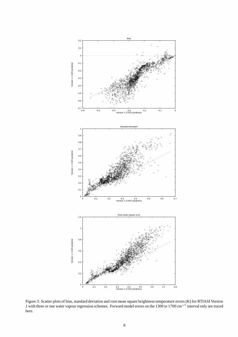
The errors show the same features as those revealed by a robust analysis of simulations for a much reduced set ofatmospheric states, the AFGL atmospheres [VS2000]: high bias and standard deviation in the H � O � � band, a structured andrelatively high standard deviation in the 8-12 � m atmospheric window, bias and random components to errors in the 9.6 � mO # and 4.3 � m CO � bands2. The v11 and v13 RTIASI model errors differ in the H � O � � band. In this spectral interval thebias and standard deviation of v11 model errors are greater than those of the v13 model. A more detailed comparison ofv11 and v13 errors in the 1300-1700 cm � interval is given by the scatter plots illustrated in Figure 3. These plots clearlyillustrate that the single water vapour predictor scheme (v11) performance is degraded most in channels where the v13 modelperformance is also poorest. This is true of bias, standard deviation and RMS. Note an approximately 1:1 mapping for biasesless than -0.2 K. v11 standard deviations are higher than v13 standard deviations over the whole range, but again, degradationis only really significant for standard deviations greater than 0.2 K.

With the exception of the H � O � � band the random component of the forward model errors (standard deviations) aresignificantly less than the instrumental noise. In the H � O � � band RTIASI version v11 random errors and instrumental noiseare comparable for both CNES scenarios, while v13 errors are only comparable with the revised CNES noise estimates

2The absolute (non-normalised) standard deviations of brightness temperature differences in the 4.3 � m band are of the order of 0.5 K, as found inVS2000. These errors are � 6 times smaller than even the revised CNES IASI instrumental noise estimates. Forward model error would not appear to bethe limiting factor for IASI retrievals in this spectral interval. The same is not true of AIRS: instrumental noise specifications are for a NE � T at 280 K ofless than 0.1 K at 2400 cm �� .

3

(O2 scenario). As mentioned above, under the (reasonable) assumption of independent instrument noise and forward modelerrors, the observation error covariance matrix O is given by the sum of the the instrumental error covariance matrix E, andthe forward model error covariance matrix F,

�� and the diagonal elements of O are given by O � �

�� . Thusif� � � 0.5

� � , as is often the case here, ‘F’ makes a relative contribution of 0.25 to the diagonals of O. Figures 1(b) and 2(b)give a useful summary of the relative contributions of instrumental and forward model error to the diagonal elements of theobservational error covariance matrix, but this is not the whole picture: interchannel correlation structures are important too.

In the upper panel of Figure 4 we illustrate the forward model error correlation matrix for the v13 RTIASI model. Toextract the correlation structures represented in this figure note that yellow indicates high correlation, blue indicates mod-erate anticorrelation, and deep orange/red indicates low correlation/approximate independance. Thus, there are correlationsbetween the 15 and 4.3 � m CO � bands ( � 650 and 2400 cm � respectively), and indeed (although poorly represented inthis figure) between Q branches in the 15 � m band. Similarly, high correlation exists between window channels (800–1000cm � , 1100–1200 cm � , � 2100 cm � and 2500 cm � spectral intervals). There is a strong correlation structure withinthe 9.6 � m O # band, and moderate anticorrelation between these errors and errors in the CO � bands and the H � O �� band.Finally, there is significant correlation structure within the � � band. The observed ‘star’ structure is related to distinct forwardmodel error characteristics in the Q, P and R-branches of the � � band. Specifically, this correlation structure indicates thaterrors in the Q-branch centre have lower correlation with the regions of low variance in the vicinity of the P and R band headsthan with errors in the P and R band wings (see Figure 1(b)).

The picture for the v11 RTIASI model is very similar. The only real difference occurs in the H � O �� error correlationstructure. Errors are more highly correlated throughout the P and R bands, and the Q-branch is actually a local minimumin forward model error. Thus the v13 ‘star’ structure is lost; there is higher, more uniform correlation across the � � band,although the Q-branch remains distinct. These features can be seen in the ‘ � � block’ of the block-F correlation matrix whichis illustrated in the lower panel of Figure 4 and which is discussed now.

The spectral structure of forward model error correlations clearly suggests that a block specification of forward modelerror covariance would capture most of the covariance structure. By block specification we mean that correlation structureswithin limited spectral intervals (e.g. spectral bands and window regions) are accounted for, outside these intervals correla-tions are neglected. A suggested block specification is illustrated for the RTIASI v11 model in the lower panel of Figure 4.With the exception of the anticorrelation of errors in the O # band and errors in the CO � bands and the H � O � � band, andcorrelations between errors in the H � O �� band and errors in the 700 – 800 cm � interval, this block approximation gives agood description of the principal correlation structures. A reordering of channels grouping the two CO � bands together andgrouping window regions together gives a computationally efficient block diagonal structure to the matrix. The accuracy ofthis block diagonal approximation will be examined in section 3.3.

As described in subsection 2.1.1 above, apodisation introduces correlation in Level 1C instrumental noise linkingchannelswithin a proximity of � 1.5 cm � (fourth-nearest neighbours). Clearly then long range correlation structures will be governedby the forward model error contribution to E+F. The significance of these correlations depends on the relative magnitudes ofinstrumental and forward model error contributions.

In Figure 5 we illustrate the observation covariance matrix��

for the v13 and v11 forward model error covariance,and the revised CNES instrumental error covariance (scenario O2). A pentadiagonal instrumental error covariance is assumed(instrumental correlations greater than 0.25) for illustrationhere, although clearly these nearest neighbour correlations cannotbe distinguished on the scale of this graph. There are significant off-pentadiagonal elements of the E+F covariance matrixin the interval around 720 cm � , the 800–1000 cm � window region, the 1050 cm � (10 � m) O # band, and the H � O ��

band. In these intervals forward model error makes a significant contribution to the observation error covariance matrix (thev11 forward model contribution in the � � band is of particular note). Elsewhere instrumental contributions dominate. Asinstrumental noise increases (e.g. if the observation error covariance is evaluated using the original CNES noise estimates)then obviously the relative contribution of forward model error to the observation error covariance decreases.

In section 3.2 we quantify changes in information content (strictly, degrees of freedom for signal) corresponding to thev11/v13 and O1/O2 forward model and instrumental error covariance scenarios. Then in section 3.3 we examine the effectof simplifying approximations to the forward model error covariance on retrieval accuracy. In addition to the block diagonalapproximation described above, we quantify the error associated with the a diagonal approximation to the forward modelerror covariance matrix. This approximation has been widely adopted in IASI performance studies to date because realisticestimates of forward model error correlations have not been available and because it simplifies and speeds up computationsradically – O(n # ) floating point operations are required to evaluate a full matrix inverse, whereas the calculation of the inverseof a diagonal is trivial and requires O(n) flops. These are clearly important considerations for IASI, where the full observationerror covariance is given by a 8641 � 8641 matrix.

A subset of 1057 channels – every eighth channel – have been selected for impact studies. As explained by Collard [10],this channel selection does not significantly modify the sampling of absorption regimes/features, so retrieval error covariancesare essentially unchanged apart from a small reduction in absolute accuracy due to a reduction in the number of degrees offreedom for signal. It does simplify calculations through the reduction of storage requirements and computation time. At theresampled resolution (2 cm � ), instrumental noise may be considered uncorrelated from channel to channel. For this reason,the instrumental error covariance is prescribed by a strict diagonal matrix. This assumption can be relaxed in future studiesas required. The current studies examine the impact of current forward model error levels and ‘long range’ forward modelerror correlations on retrieval accuracy and measurement information content.

4

2.2 Jacobian error estimates

Forward model error is taken into account explicitly in the retrieval process – the relative weights of the a priori informationand observations in determining analysis increments are governed by their respective error characteristics. The variationalframework makes the implicit assumption that fast model Jacobians are exact. This hypothesis clearly needs to be validated.

One approach to validating fast model tangent linear Jacobians is to compare them with brute force (finite difference)Jacobians calculated using a line-by-line model3. Errors in RTIASI version v13 temperature and water vapour Jacobians wereevaluated in this manner in VS2000 for the AFGL tropical and sub-arctic winter atmospheres on three targeted wavenumbersubintervals: 645-800 cm � , 885-915 cm � and 1300-1450 cm � . This study showed that modelled temperature Jacobians�� were generally very satisfactory (errors typically � 5 � ), but that water vapour Jacobians

�� wereconsiderably less well modelled. In the AFGL1 atmosphere errors of the order of 10-40 � were found in the magnitude ofwater vapour Jacobians, although this was much improved in the AFGL5 atmosphere. Larger errors still were found in thev02 release in cases where switching between predictor schemes gave rise to large discontinuities in modelled Jacobians.This problem is reduced, but not completely eliminated in the v13 release (discontinuities still occur for some Jacobians, butare smaller in magnitude).

The corresponding analysis has been made for the RTIASI version v11 Jacobians. The accuracy of modelled temperatureJacobians remains essentially unchanged. A small improvement in temperature Jacobians in the 750-800 cm � interval isnoted for AFGL1. A small degradation is noted in the same interval for AFGL5. Significant improvements in the accuracyof modelled water vapour Jacobians are found in both the 885-915 cm � and the 1300-1450 cm � interval for the AFGL1atmosphere. Again, a degredation in accuracy is found for the AFGL5 atmosphere. This implies that the v11 scheme modelswater vapour absorption better than the v13 scheme in both the window region and the H � O � � band in the case of the AFGL1atmosphere, but worse in the case of the AFGL5 atmosphere. Extrapolation of these results to ‘humid’ and ‘dry’ atmospheresis not recommended (!)

Comparisons of the maximum relative errors in RTIASI v11 and v13 water vapour Jacobians for the AFGL1 and AFGL5atmospheres on the 1300-1450 cm � interval are illustrated in Figure 6. Strictly, the error represented is the maximum relativeerror for Jacobian elements whose value is � 50 � maximum Jacobian element for the given channel and atmosphere, andthe error is signed: positive errors indicate GENLN2 � RTIASI (in terms of the absolute value of the Jacobian elements),conversely negative errors indicate GENLN2 � RTIASI. The Jacobians considered are essentially well behaved, smoothfunctions i.e. there are none of the gross errors (discontinuities) of the v02 release. Thus the maximum relative errorcharacterises the typical magnitude of errors in the region of maximum sensitivity on a channel by channel basis.

The improvement in the v11 AFGL1 water vapour Jacobians is clear - errors are generally of the order of 10 � as opposedto 10-30 � for the v13 scheme. However, the degradation in the AFGL5 case is as evident. Errors are of the order of 20 �as compared with 5-10 � for the v13 scheme. Note however that the AFGL5 atmosphere is particularly dry; sensitivity toperturbations in the analysis variable ln(q) (d �� (q)= � . � ) is therefore significantly lower than that found in the AFGL1 case(i.e. the absolute values of the water vapour Jacobians are smaller).

The impact of errors in modelled temperature and water vapour Jacobians on retrieval accuracy is described in section 3.4.

3Profile perturbations must be small enough to ensure a linear approximation is valid.5

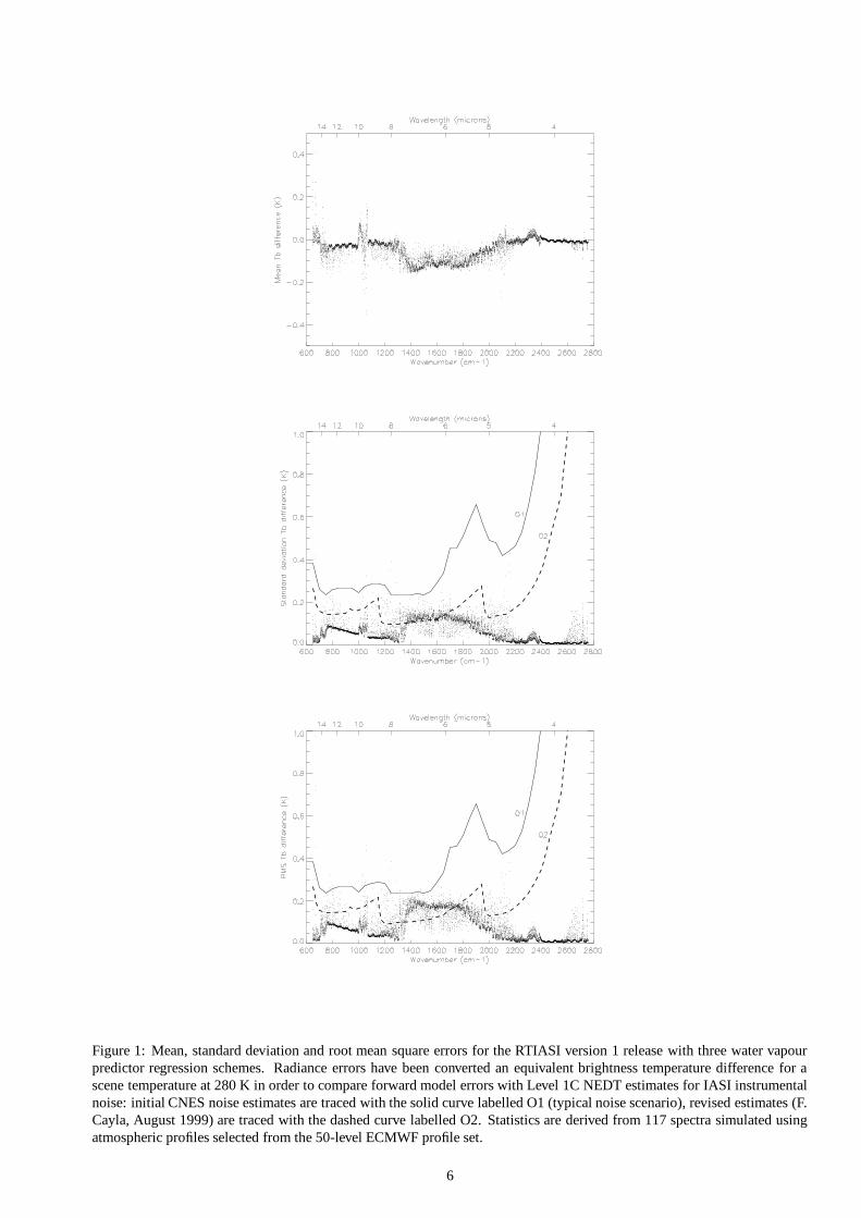
Figure 1: Mean, standard deviation and root mean square errors for the RTIASI version 1 release with three water vapourpredictor regression schemes. Radiance errors have been converted an equivalent brightness temperature difference for ascene temperature at 280 K in order to compare forward model errors with Level 1C NEDT estimates for IASI instrumentalnoise: initial CNES noise estimates are traced with the solid curve labelled O1 (typical noise scenario), revised estimates (F.Cayla, August 1999) are traced with the dashed curve labelled O2. Statistics are derived from 117 spectra simulated usingatmospheric profiles selected from the 50-level ECMWF profile set.

6

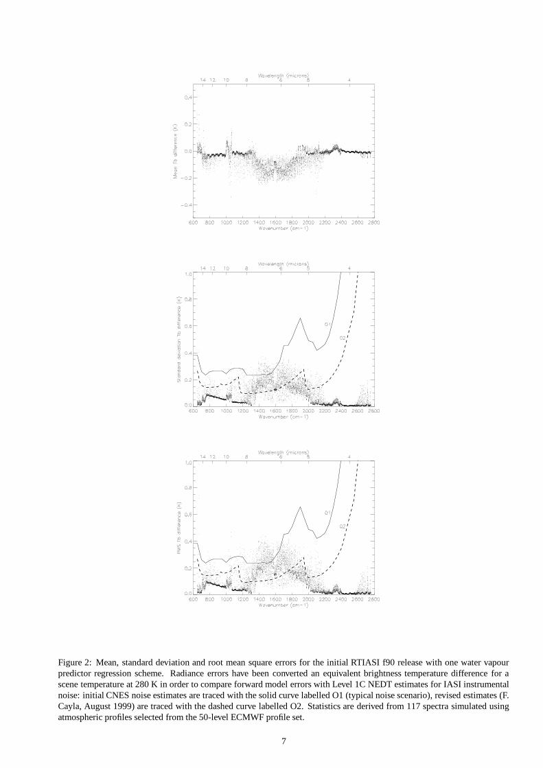
Figure 2: Mean, standard deviation and root mean square errors for the initial RTIASI f90 release with one water vapourpredictor regression scheme. Radiance errors have been converted an equivalent brightness temperature difference for ascene temperature at 280 K in order to compare forward model errors with Level 1C NEDT estimates for IASI instrumentalnoise: initial CNES noise estimates are traced with the solid curve labelled O1 (typical noise scenario), revised estimates (F.Cayla, August 1999) are traced with the dashed curve labelled O2. Statistics are derived from 117 spectra simulated usingatmospheric profiles selected from the 50-level ECMWF profile set.

7

-0.7

-0.6

-0.5

-0.4

-0.3

-0.2

-0.1

0

0.1

0.2

-0.6 -0.5 -0.4 -0.3 -0.2 -0.1 0

Ver

sion

1 1

H2O

pre

dict

or

Version 1 3 H2O predictors

Bias

0

0.1

0.2

0.3

0.4

0.5

0.6

0.7

0.8

0.9

1

0 0.1 0.2 0.3 0.4 0.5 0.6 0.7

Ver

sion

1 1

H2O

pre

dict

or


Standard deviation

0

0.2

0.4

0.6

0.8

1

1.2

0 0.1 0.2 0.3 0.4 0.5 0.6 0.7 0.8

Ver

sion

1 1

H2O

pre

dict

or


Root mean square error

Figure 3: Scatter plots of bias, standard deviation and root mean square brightness temperature errors (K) for RTIASI Version1 with three or one water vapour regression schemes. Forward model errors on the 1300 to 1700 cm � interval only are tracedhere.

8

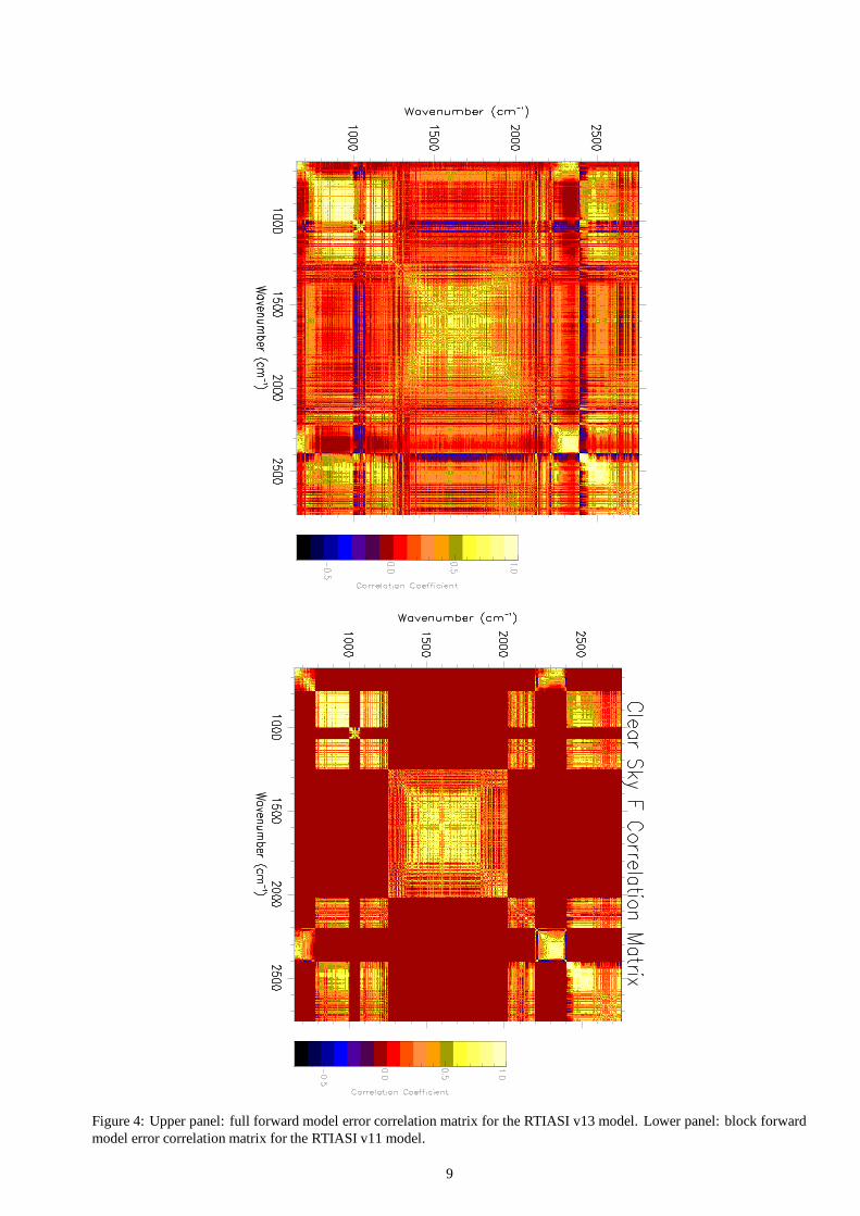
Figure 4: Upper panel: full forward model error correlation matrix for the RTIASI v13 model. Lower panel: block forwardmodel error correlation matrix for the RTIASI v11 model.

9

Figure 5: Observational error covariance matrices for RTIASI v13 and v11 models (upper an lower panels respectively).In both cases the instrumental noise is given by the revised (O2) CNES Level 1C estimates. Covariance in units of K �

(normalised brightness temperature differences for a scene temperature of 280 K).

10

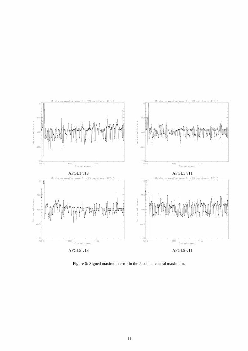
AFGL1 v13 AFGL1 v11

AFGL5 v13 AFGL5 v11

Figure 6: Signed maximum error in the Jacobian central maximum.

11

3 Impact of fast model errors on retrieval error covariances

3.1 Methodology

The impact of forward model errors on retrieval accuracy is assessed within a linear retrieval framework. The analysispresented here is a direct application of the methodology used by Watts and McNally [11] to assess the sensitivity of aminimum variance retrieval scheme to the values of its principal parameters and by Collard [10] to assess the impact ofundetected cloud on IASI retrievals. This methodology is outlined briefly here.

In a minimum variance retrieval scheme the best estimate of atmospheric state�� is found by minimising the cost function

J(x):

� � � � � � �� )�� ) � � � �� (1)

where x � is the a priori estimate of atmospheric state, with associated error covariance B, the y � are observations, and � (x)is the forward operator mapping the state x into observation space. y- � (x) has an associated error covariance O which iscomprised of two terms or error sources: E, the instrumental error covariance and F, the forward model error covariance.These errors are assumed to be independent, thus

�� -�.

In the linear or weakly nonlinear case analysis increments�� are given by:

�� ) � � �� ) � � �� (2)�� ) � � � � � � � � � � ) � ��

W is known as the gain or weight matrix of the analysis. The rows of W describe how the departures y- � (x � ) are mappedinto analysis increments.

If the true atmospheric state is given by x ) , then in the linear case Equation 2 can be expressed as:

�� ) ��

��"!�# � (3)

where R = W�� is the averaging kernel or model resolution matrix, and

!%$is the realisation of instrumental and for-

ward model noise for the given observations y and mapping � (x � ). An appropriate analysis of the resolution matrix yieldsimportant information on retrieval characteristics and is discussed below.

Equation 3 may be rearranged to give an expression for the difference between the analysis and the true atmospheric state�� ) :

�� )� �& � � � � � �� ) �

�'�(! # � (4)

which may in turn be used to estimate the error covariance for an ensemble of retrievals A (the a posteriori error covariance):

+ � )+* � �� ) � �� ) � )-, �� & � �"�� & � �"�� ) �.�� ) � (5)

where)

[ ] denotes statistical expectation. The retrieval error covariance is comprised of two terms. The latter, WOW )describes the propogation of measurement noise and forward model errors into retrieved states

�� , while the former describeshow errors in the a priori estimate of atmospheric state are propogated into the retrieval when (as) the a priori information isused to ‘fill out’ that profile information which cannot be deduced from observations. For this reason this term is describedas the null space error by Rodgers [12].

If now we consider an ensemble of retrievals where an observation error covariance O has been assumed in W, but thetrue observation error covariance is O / , then the retrieval error covariance is given by:

+ / � �& � �"� � � � � ��& � �"� � � � ) �.�� / � ) �+ / � +�� / � � � � ) � (6)

Thus, errors in the assumed observation error covariance matrix are seen to give an additional contribution to the propogatedmeasurement error – the minimum variance solution or optimal retrieval requires O 0 O / .

In a similar manner, if an ensemble of retrievals are performed assuming a Jacobian� � � , when in fact

� � � / is the trueJacobian, then the retrieval error covariance is given by:

+ / � ��& � �"� � � / � � �& � �(� � � / � ) �.�� )1� (7)

Retrieval errors are increased through the incorrect mapping of a priori information: the minimum variance solution requires�� 0 �� / .

12

3.1.1 Measures for retrieval characterisation

Comparison of a priori and a posteriori error covariance matrices gives a measure of the benefit of the assimilation of thegiven observation type. This ‘benefit’ may be assessed through comparison of the a priori and a posteriori variances andthrough measures such as the degrees of freedom for signal and/or measurement information content [13]. In the studiespresented here we mainly focus on the modification of the retrieval variance (or standard deviation) – i.e. the diagonalelements of the retrieval error covariance matrix A. In particular, we will quantify the increase in retrieval variance due tosimplifying approximations (block diagonal and diagonal approximations) to the full forward model error covariance matrixand due to errors in modelled Jacobians through the relations defined in Equations 6 and 7 above. However, we also evaluatethe modification of the degrees of freedom for signal due to approximations to the forward model error covariance and dueto errors in modelled Jacobians following the method outlined by Rodgers [13]. Specifically,

� �� & � + / � � � � �& � � �� + � � �� ) � � (8)

Four observation error covariance scenarios have been considered (v11,v13) � (O1,O2) for two relatively extreme atmosphericstates (A1 0 AFGL1 tropical and A5 0 AFGL5 sub-arctic winter atmospheres). Two linearisation points have been consideredto give some measure of the state dependence of retrieval characteristics. The treatment of nonlinearity errors is beyond thescope of this report (see Eyre [14], Eyre and Collard [15]).

Often results can be better understood in the light of information deduced from an analysis of the corresponding resolutionmatrix. For this reason, we begin the presentation of results from these impact studies with a discussion of the degrees offreedom for signal and effective vertical resolution of retrievals for the different error covariance and atmospheric statescenarios. The measures derived from the resolution matrix in order to characterise the information content and verticalresolution of the retrieval are:

� Tr(R) and components R��

: if retrievals are performed using the optimal gain matrix W, the trace of the resolutionmatrix may be interpreted in terms of the number of degrees of freedom for signal in the retrieval [13], or equivalently,as the total effective number of constraints imposed on the retrieval by the observed data [16]. Purser and Huang [16]extend this concept to define a measure of local data density � � � � � �� and effective vertical resolution ( � �� ).As this definition of vertical resolution has been used in previous IASI retrieval characterisation studies [17], it is themeasure of vertical resolution choosen for illustration here. For an ideal observation R=I, the identity matrix, andTr(R)=dim(x). For reference, the state vector considered has 75 elements: temperature on 43 pressure levels, surfaceair and skin temperature, humidity on 28 pressure levels, surface air humidity and surface pressure.

� Eigenvalue/eigenvector decomposition: the rows of the resolution matrix describe how the departures x � -x � aresmoothed in the analysis increments

�� -x � , while the columns of R describe how a perturbation at one profile levelwill be redistributed in analysis increments. An eigenvalue/eigenvector decomposition of the resolution matrix allows(vertically correlated) structures in departures which can be retrieved from observations to be identified [12] providingan alternative method to summarize the structure and smoothing characteristics of the resolution matrix.

A single a priori error covariance matrix B is used throughout these studies. This is the ECMWF 40-level backgrounderror covariance matrix interpolated onto RTIASI model levels which has been used in previous retrieval characterisationstudies [10][17]. The a priori error specification has an important role in determining the relative weight of observations inanalysis increments, and in determining how increments are smoothed in the vertical: estimates of degrees of freedom forsignal and retrieval error covariance depend on the detail of B. We reiterate then that results apply to retrievals/analyses in anoperational/NWP framework where the a priori estimate of atmospheric state is reasonably well constrained, particularly forthe tropospheric temperature field. No evaluation of the sensitivity of results to the specification of B has been undertakenhere.

13

Simulation DFS full Simulation DFS fullv11 O1 A5 10.3 v11 O1 A1 16.3v13 O1 A5 10.4 v13 O1 A1 16.4v11 O2 A5 12.7 v11 O2 A1 21.5v13 O2 A5 12.8 v13 O2 A1 21.6

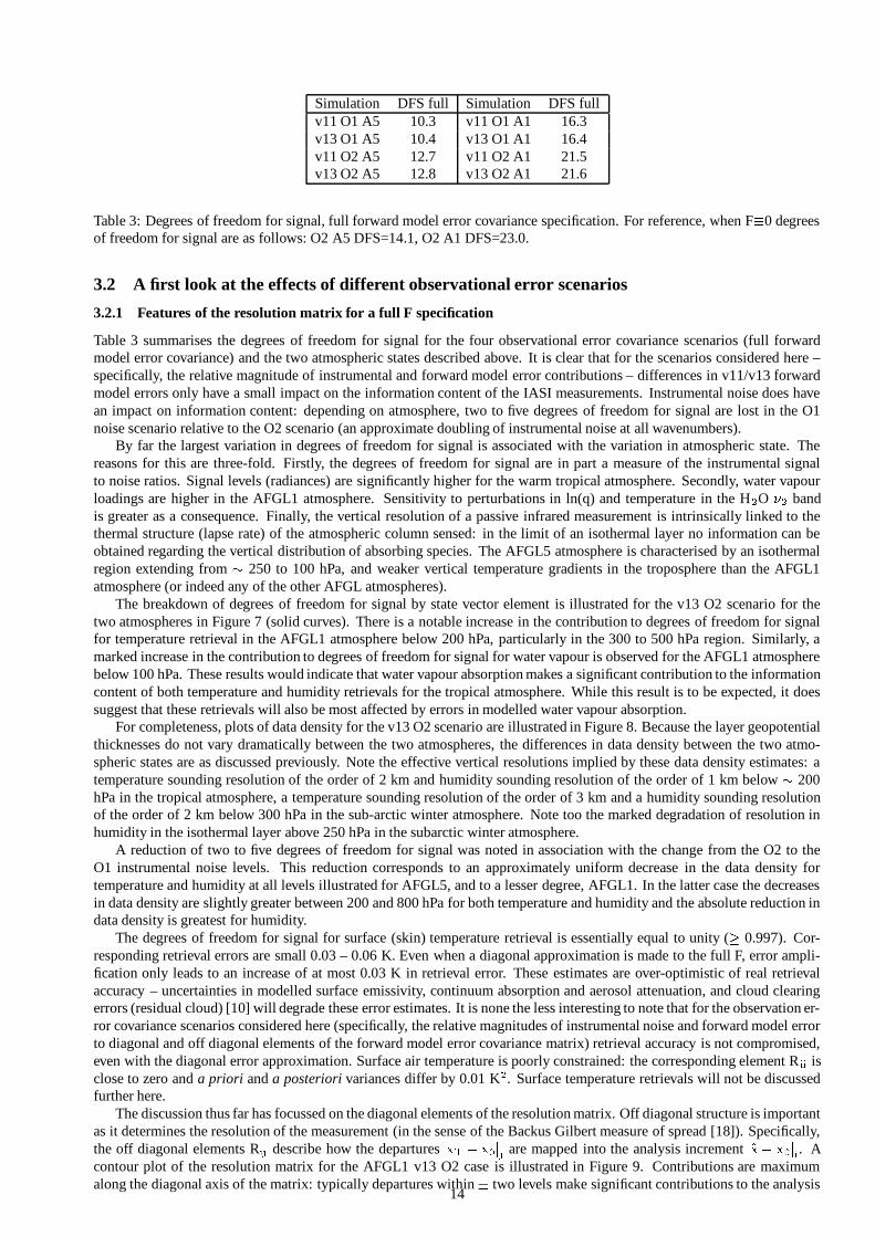
Table 3: Degrees of freedom for signal, full forward model error covariance specification. For reference, when F 0 0 degreesof freedom for signal are as follows: O2 A5 DFS=14.1, O2 A1 DFS=23.0.

3.2 A first look at the effects of different observational error scenarios

3.2.1 Features of the resolution matrix for a full F specification

Table 3 summarises the degrees of freedom for signal for the four observational error covariance scenarios (full forwardmodel error covariance) and the two atmospheric states described above. It is clear that for the scenarios considered here –specifically, the relative magnitude of instrumental and forward model error contributions – differences in v11/v13 forwardmodel errors only have a small impact on the information content of the IASI measurements. Instrumental noise does havean impact on information content: depending on atmosphere, two to five degrees of freedom for signal are lost in the O1noise scenario relative to the O2 scenario (an approximate doubling of instrumental noise at all wavenumbers).

By far the largest variation in degrees of freedom for signal is associated with the variation in atmospheric state. Thereasons for this are three-fold. Firstly, the degrees of freedom for signal are in part a measure of the instrumental signalto noise ratios. Signal levels (radiances) are significantly higher for the warm tropical atmosphere. Secondly, water vapourloadings are higher in the AFGL1 atmosphere. Sensitivity to perturbations in ln(q) and temperature in the H � O � � bandis greater as a consequence. Finally, the vertical resolution of a passive infrared measurement is intrinsically linked to thethermal structure (lapse rate) of the atmospheric column sensed: in the limit of an isothermal layer no information can beobtained regarding the vertical distribution of absorbing species. The AFGL5 atmosphere is characterised by an isothermalregion extending from � 250 to 100 hPa, and weaker vertical temperature gradients in the troposphere than the AFGL1atmosphere (or indeed any of the other AFGL atmospheres).

The breakdown of degrees of freedom for signal by state vector element is illustrated for the v13 O2 scenario for thetwo atmospheres in Figure 7 (solid curves). There is a notable increase in the contribution to degrees of freedom for signalfor temperature retrieval in the AFGL1 atmosphere below 200 hPa, particularly in the 300 to 500 hPa region. Similarly, amarked increase in the contribution to degrees of freedom for signal for water vapour is observed for the AFGL1 atmospherebelow 100 hPa. These results would indicate that water vapour absorption makes a significant contribution to the informationcontent of both temperature and humidity retrievals for the tropical atmosphere. While this result is to be expected, it doessuggest that these retrievals will also be most affected by errors in modelled water vapour absorption.

For completeness, plots of data density for the v13 O2 scenario are illustrated in Figure 8. Because the layer geopotentialthicknesses do not vary dramatically between the two atmospheres, the differences in data density between the two atmo-spheric states are as discussed previously. Note the effective vertical resolutions implied by these data density estimates: atemperature sounding resolution of the order of 2 km and humidity sounding resolution of the order of 1 km below � 200hPa in the tropical atmosphere, a temperature sounding resolution of the order of 3 km and a humidity sounding resolutionof the order of 2 km below 300 hPa in the sub-arctic winter atmosphere. Note too the marked degradation of resolution inhumidity in the isothermal layer above 250 hPa in the subarctic winter atmosphere.

A reduction of two to five degrees of freedom for signal was noted in association with the change from the O2 to theO1 instrumental noise levels. This reduction corresponds to an approximately uniform decrease in the data density fortemperature and humidity at all levels illustrated for AFGL5, and to a lesser degree, AFGL1. In the latter case the decreasesin data density are slightly greater between 200 and 800 hPa for both temperature and humidity and the absolute reduction indata density is greatest for humidity.

The degrees of freedom for signal for surface (skin) temperature retrieval is essentially equal to unity ( � 0.997). Cor-responding retrieval errors are small 0.03 – 0.06 K. Even when a diagonal approximation is made to the full F, error ampli-fication only leads to an increase of at most 0.03 K in retrieval error. These estimates are over-optimistic of real retrievalaccuracy – uncertainties in modelled surface emissivity, continuum absorption and aerosol attenuation, and cloud clearingerrors (residual cloud) [10] will degrade these error estimates. It is none the less interesting to note that for the observation er-ror covariance scenarios considered here (specifically, the relative magnitudes of instrumental noise and forward model errorto diagonal and off diagonal elements of the forward model error covariance matrix) retrieval accuracy is not compromised,even with the diagonal error approximation. Surface air temperature is poorly constrained: the corresponding element R � � isclose to zero and a priori and a posteriori variances differ by 0.01 K � . Surface temperature retrievals will not be discussedfurther here.

The discussion thus far has focussed on the diagonal elements of the resolution matrix. Off diagonal structure is importantas it determines the resolution of the measurement (in the sense of the Backus Gilbert measure of spread [18]). Specifically,the off diagonal elements R �

�describe how the departures � ) ��

� �are mapped into the analysis increment

��

� � . Acontour plot of the resolution matrix for the AFGL1 v13 O2 case is illustrated in Figure 9. Contributions are maximumalong the diagonal axis of the matrix: typically departures within � two levels make significant contributions to the analysis

14

increment for a given level. Averaging kernel widths at half maximum (FWHM) are consistent with the effective verticalresolution estimates given above. Note however how humidity departures contribute to tropospheric temperature increments,reflecting the fundamental ambiguity in interpretation of radiances from the � � H � O band (absorption by a variable gas).

Structures are similar for the AFGL5 atmosphere. The vertical resolution of the measurements is lower (this may begauged qualitatively from the density of the contour lines in the resolution plot, and is again consistent with effective verticalresolution estimates) although the contribution of water vapour departures to temperature increments is reduced.

3.2.2 Comparison of the resolution matrices for the three F scenarios

The diagonal elements R � � of the resolution matrices for block diagonal and diagonal forward model error covariance matrixapproximations are also illustrated in Figure 7 (dashed and dotted curves respectively). In all cases there is no significantchange to the diagonal elements of R on the introduction of the block diagonal approximation. There are some small changesto the diagonal components of R in the case of the diagonal approximation – principally a reduction in the ‘resolution’ ofhumidity in the mid troposphere and a small increase in the ‘resolution’ of upper stratospheric temperature (not shown). Thesignificance of this increase is questionable: eigenvalue/eigenvector truncation tests indicate this effect is associated with/dependent on the smallest eigenvalue/eigenvector components of the innovation error covariance ( � � �� ) � � � � ) � .The off-diagonal structure of the resolution matrices has also been visualised graphically for the three forward model errorcovariance scenarios (as in Figure 9). Qualitatively the structures are very similar – in particular, the temperature/watervapour mixing in temperature retrievals is a consistent feature for all cases.

A better measure of differences can be gained through comparison of the eigenvectors of the resolution matrices. Theleading eigenvectors of the resolution matrix have been examined for the three forward model error covariance scenarios(full, block, diagonal error covariance matrices) for the v13 O2 observational error covariance scenario. Modifications inthe leading eigenvectors of R are generally small for the full and block approximations. The most significant differences areassociated with temperature structures at pressures less than 100 hPa ( � 16 – 17 km). It is thought that this is due to the factthat anticorrelations between errors in the O # band and errors in the CO � and H � O bands are not taken into account in theblock diagonal specification of the F matrix (unmodelled correlations between the CO � bands and the H � O �� band may alsoplay a role). Small modifications to the resolution of water vapour between 100 and 300 hPa are also observed. In one case(5

��

leading eigenvector, AFGL1) there are significant differences in lower tropospheric temperature and humidity in the 400to 100 hPa region.

The eigenvalues for the resolution matrix for the diagonal F approximation are generally topologically similar to those forthe full and block cases. However, the eigenvectors often present significant differences in the magnitude of the ‘smoothing’structures. Structures can also be displaced (translation in the vertical). This, and the modification of the diagonal elements ofthe resolution matrix indicates that the diagonal F approximation can give quite different retrieval resolution and smoothingcharacteristics. We will return to this point in section 3.4.

The differences in the eigenvectors of R for full, block diagonal and diagonal F matrices are qualitatively similar forthe AFGL1 and AFGL5 atmospheres. The fact that there are more leading eigenvectors of the full R matrix which are‘temperature only’ modes for the AFGL5 atmosphere is however of note (Eigenvectors 1, 4, 5, 7, (9, 11) are all ‘temperatureonly’ modes, as compared to eigenvectors 8, 10, (11, 16, 17, 21) ... for AFGL1). This is consistent with the weakertemperature/water vapour mixing in temperature retrivals noted previously for the AFGL5 atmosphere.

3.2.3 Comparison of the retrieval variance for the three F ‘truth’ scenarios

The retrieval error covariance matrix has also been compared for the three forward model error covariance ‘truth’ scenarios.No significant change to the retrieval variance was found: for a given atmosphere and instrumental noise scenario, the retrievalvariances were equivalent for all three forward model error scenarios for all practical purposes. Throughout the followingsections retrieval variances and standard deviations will be illustrated for various approximations to the forward model errorcovariance matrix and for different Jacobian error scenarios. Unless stated explicitly, the full forward model error covarianceis assumed as truth in all comparisons.

15

Figure 7: Contributions to degrees of freedom for signal for temperature and humidity for the AFGL1 tropical atmosphere(upper panels) and AFGL5 sub-arctic winter atmosphere (lower panels). Observational error covariance is given by the v13O2 scenario. The solid curve illustrates the contributions to the degrees of freedom for signal for a full forward model errorcovariance specification. The dashed curve illustrates the diagonal elements of the resolution matrix for a block diagonalforward model error covariance matrix. The dotted curve illustrates the diagonal elements of the resolution matrix for adiagonal forward model error covariance matrix. Note the marked increases in the degrees of freedom for signal for mid andlower tropospheric temperature and tropospheric humidity in the tropical atmosphere.

16

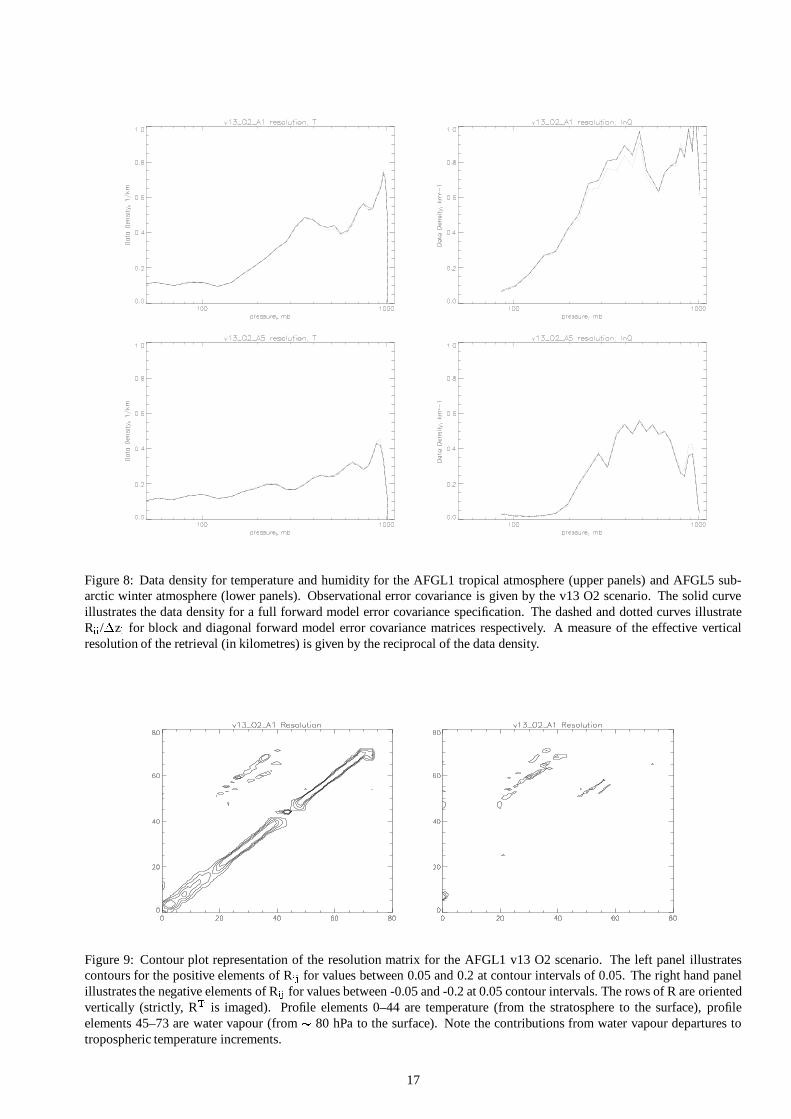
Figure 8: Data density for temperature and humidity for the AFGL1 tropical atmosphere (upper panels) and AFGL5 sub-arctic winter atmosphere (lower panels). Observational error covariance is given by the v13 O2 scenario. The solid curveillustrates the data density for a full forward model error covariance specification. The dashed and dotted curves illustrateR � � / � z � for block and diagonal forward model error covariance matrices respectively. A measure of the effective verticalresolution of the retrieval (in kilometres) is given by the reciprocal of the data density.

Figure 9: Contour plot representation of the resolution matrix for the AFGL1 v13 O2 scenario. The left panel illustratescontours for the positive elements of R �

�for values between 0.05 and 0.2 at contour intervals of 0.05. The right hand panel

illustrates the negative elements of R ��

for values between -0.05 and -0.2 at 0.05 contour intervals. The rows of R are orientedvertically (strictly, R ) is imaged). Profile elements 0–44 are temperature (from the stratosphere to the surface), profileelements 45–73 are water vapour (from � 80 hPa to the surface). Note the contributions from water vapour departures totropospheric temperature increments.

17

3.3 Impact of simplifying approximations to the forward model error covariance matrix

We now consider the error inherent in two simplifying assumptions to the structure of the full forward model error covariancematrix: block diagonal and diagonal F matrices. As discussed previously, if an observation error covariance O is assumedin retrievals, i.e. assumed in the calculation of the gain matrix W, the retrieval error covariance is increased by a term� � � � � / � � ) describing how the incorrect specification of the observation error covariance is mapped into retrievals.

The standard deviations of an ensemble of temperature and humidity retrievals are illustrated for the v13 O2 observationerror covariance scenario and the two AFGL atmospheres in Figure 10. Full block and diagonal forward model error scenariosare illustrated as previously with full, dashed and dotted curves. The standard deviations of the a priori information areillustrated by the dot-dashed curve.

It is immediately apparant that the block diagonal approximation to the forward model error covariance matrix sucessfullycaptures all relevant correlation structure. The error introduced by this approximation is negligible for all practical purposesand this is true of all the other observational error covariance scenarios considered in this study. There is a small – arguablytolerable – degradation in retrieval accuracy associated with the diagonal approximation to the forward model error covariancematrix. This error is largest for the AFGL1 mid-troposphere temperature retrievals and the AFGL5 upper tropospherichumidity retrievals.

The breakdown of the null and propagated measurement error contributions for these cases are illustrated in Figure 11.The propagated measurement error contributions to the retrieval variance for full, block and diagonal forward model errorscenarios are illustrated as previously with full, dashed and dotted curves. The null space contributions to the retrievalvariance are illustrated by the dot-dashed curve. Null and measurement error contributions are comparable below 200 hPain the AFGL1 case, and the error contribution due to the diagonal approximation is significant for temperature retrievalsin the mid troposphere. Null space error dominates the error budget for the AFGL5 atmosphere, although the diagonalapproximation makes a significant contribution to humidity measurement errors in the lower and upper troposphere. Notethe higher measurement information content for the AFGL1 atmosphere leads to lower null space contributions, and overall,lower retrieval errors.

While the absolute magnitude of the error due to the diagonal F approximation is small, it can be a significant fraction ofthe reduction in error/uncertainty in the atmospheric state. The reduction in variance on assimilation of (IASI) observationscan be usefully measured by the fraction of unexplained variance

+ � � � � � � . For the AFGL1 atmosphere, the fraction ofunexplained variance is of � 20 � for both temperature and humidity below 200 hPa. The diagonal forward model errorapproximation increases the fraction of unexplained variance by 5 to 10 � . For comparison, the fraction of unexplainedvariance in the AFGL5 temperature retrieval is of the order of 60 � in the upper troposphere, decreasing to 40 � in the lowertroposphere. The fraction of unexplained variance in humidity is of the order of 20 � between 300 and 700 hPa, but increasesrapidly above and below. The diagonal forward model error approximation increases the fraction of unexplained variance by� 5 � .

Obviously, where the information content of observations allows a significant reduction in variance, then the retrieval(retrieval accuracy) is more sensitive to the detail of the forward model error covariance specification. In the cases illustratedhere the degradation is tolerable. Clearly one does not want the situation where the error amplification is such that theassimilation of observations results in a retrieval with greater uncertainty than the a priori state.

In Figure 12 we illustrate an equivalent analysis of retrieval standard deviations for the v11 O2 observation error covari-ance scenario. There is a clear increase in the errors in tropospheric temperature and humidity retrievals associated withdiagonal F approximation for both atmospheres. Mid tropospheric temperature retrievals and humidity retrievals in the 100-300 hPa region are most affected in the AFGL1 atmosphere – in these regions propagated measurement errors are greaterthan or equal to null space errors, and the fraction of unexplained variance increases by � 20 to 40 � for the diagonal Fapproximation. In the AFGL5 atmosphere humidity retrievals are significantly degraded in the 200 to 300 and 800 to 1000hPa regions (amplification of the propagated measurement error structures illustrated in Figure 11(d)). In these intervalsthe fraction of unexplained variance increases by 20 to 40 � for the diagonal F approximation. Increases in the fraction ofunexplained variance for temperature are of the order of 5 to 10 � at tropospheric levels.

Finally, in Figure 13 we illustrate retrieval errors for the v11 O1 observation error covariance scenario. The increasedinstrumental noise gives rise to a slight degradation in retrieval accuracy for temperature and humidity at all levels (ascompared to the v11 O2 scenario). With the increased weight of the diagonal elements of the observation error covariancematrix (due to the increase in instrumental noise) the diagonal error assumption is an increasingly reasonable approximationto the full observation error covariance matrix. The impact of the diagonal approximation on retrieval accuracy is small –propagated measurement errors are less than null space errors everywhere (with the exception of the 300 to 400 hPa regionfor AFGL1 temperature retrievals, where null and measurement errors are equal in magnitude). Errors are smaller still forthe v13 O1 scenario (not illustrated) also for this reason.

When retrievals are performed with a suboptimal gain matrix retrieval accuracy is compromised and there is a corre-sponding reduction in measurement information content or degrees of freedom for signal. To complete the discussion above,Table 4 extends the tabulation of degrees of freedom for signal for the full F matrix given in Table 3 to the degrees of freedomfor signal for the block diagonal and diagonal approximations to forward model error covariance matrix. Again, reductionsin the degrees of freedom for signal are small – � 0.2 in all cases – for the block diagonal approximation. Reductions indegrees of freedom for signal for the diagonal approximation range from 0.3 to 3.1, and are most marked for the v11 forwardmodel in the O2 instrumental noise scenario.

18

Simulation DFS full DFS block DFS diag Simulation DFS full DFS block DFS diagv11 O1 A5 10.3 10.2 9.5 v11 O1 A1 16.3 16.2 15.5v13 O1 A5 10.4 10.3 10.1 v13 O1 A1 16.4 16.3 16.1v11 O2 A5 12.7 12.5 10.0 v11 O2 A1 21.5 21.3 18.2v13 O2 A5 12.8 12.6 11.4 v13 O2 A1 21.6 21.4 20.1

Table 4: Degrees of freedom for signal for the full forward model error covariance specification and block diagonal anddiagonal approximations.

In conclusion then, where the diagonal terms are the dominant elements in the observational error covariance matrix (e.g.E � � /F � � � 4:1) then a diagonal approximation to the forward model error covariance matrix – the unique source of long rangeerror correlations – is adequate. The diagonal approximation might be considered unsatisfactory in cases where forwardmodel and instrumental noise are comparable in magnitude in a spectral interval which is being given significant weightin determining analysis increments - water vapour absorption in the � � band in the v11 O2 A1 scenario, for example. Inthis situation a block diagonal assumption appears a very good approximation to the full error covariance matrix and thiswill be true whenever errors present the same type of spectral/spectroscopic correlation structures as those considered here.Given that there may be modifications to the resolution matrix (averaging kernels) on passing from a full/block to a diagonalspecification of the forward model error covariance matrix, it is probably well worth performing off-line channel selectionstudies with full or block F matrices.

19

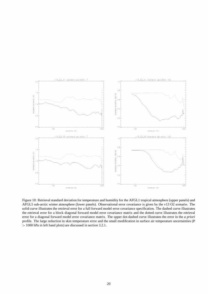
Figure 10: Retrieval standard deviation for temperature and humidity for the AFGL1 tropical atmosphere (upper panels) andAFGL5 sub-arctic winter atmosphere (lower panels). Observational error covariance is given by the v13 O2 scenario. Thesolid curve illustrates the retrieval error for a full forward model error covariance specification. The dashed curve illustratesthe retrieval error for a block diagonal forward model error covariance matrix and the dotted curve illustrates the retrievalerror for a diagonal forward model error covariance matrix. The upper dot-dashed curve illustrates the error in the a prioriprofile. The large reduction in skin temperature error and the small modification in surface air temperature uncertainties (P� 1000 hPa in left hand plots) are discussed in section 3.2.1.

20

Figure 11: Null and propagated measurement error contributions to the retrieval variance for temperature and humidity forthe AFGL1 tropical atmosphere (upper panels) and AFGL5 sub-arctic winter atmosphere (lower panels). Observational errorcovariance is given by the v13 O2 scenario. The solid curve illustrates the measurement contribution to retrieval variance fora full forward model error covariance specification. The dashed curve illustrates this measurement contribution for a blockdiagonal forward model error covariance matrix and the dotted curve illustrates this measurement contribution for a diagonalforward model error covariance matrix. The dot-dashed curve illustrates the null space contribution to retrieval variance.

21

Figure 12: Retrieval standard deviation for temperature and humidity for the AFGL1 tropical atmosphere (upper panels) andAFGL5 sub-arctic winter atmosphere (lower panels). Observational error covariance is given by the v11 O2 scenario. Thesolid curve illustrates the retrieval error for a full forward model error covariance specification. The dashed curve illustratesthe retrieval error for a block diagonal forward model error covariance matrix and the dotted curve illustrates the retrievalerror for a diagonal forward model error covariance matrix. The upper dot-dashed curve illustrates the error in the a prioriprofile.

22

Figure 13: Retrieval standard deviation for temperature and humidity for the AFGL1 tropical atmosphere (upper panels) andAFGL5 sub-arctic winter atmosphere (lower panels). Observational error covariance is given by the v11 O1 scenario. Thesolid curve illustrates the retrieval error for a full forward model error covariance specification. The dashed curve illustratesthe retrieval error for a block diagonal forward model error covariance matrix and the dotted curve illustrates the retrievalerror for a diagonal forward model error covariance matrix. The upper dot-dashed curve illustrates the error in the a prioriprofile.

23

Simulation DFS R � DFS R � Simulation DFS R � DFS R �

v11 O1 A5 10.3 9.1 v11 O1 A1 16.3 12.2v13 O1 A5 10.4 9.1 v13 O1 A1 16.4 12.5v11 O2 A5 12.7 11.1 v11 O2 A1 21.5 14.9v13 O2 A5 12.8 11.0 v13 O2 A1 21.6 15.8

Table 5: Degrees of freedom for signal for the 1057 channel full F matrix simulations R � , and 163 channel reference (truth)Jacobian simulations R � =W.H, W 0 W(H).

3.4 Impact of errors in modelled Jacobians

In this section we consider the impact of errors in fast model Jacobian on retrieval accuracy. As described previously, Jacobianerrors impact on the null space error, giving a non-optimal propagation (an incorrect mapping/interpretation) of a priori errorin the retrieval.

In order to evaluate the impact of errors in RTIASI Jacobians GENLN2 finite difference Jacobian calculations are takenas truth. To date GENLN2 Jacobians have only been calculated on three targetted subintervals: 645 – 805 cm � , 885 –915 cm � and 1300 – 1450 cm � . Moreover, water vapour Jacobians have not been evaluated for the first subinterval. Thecomparisons illustrated here are performed for the 2 cm � sampled spectra on these three subintervals: 163 channels areanalysed in total, reference water vapour Jacobians exist for 86 channels. Only ‘well-behaved’ water vapour Jacobians areconsidered, but relative errors of 10-40 � in the magnitude of Jacobian elements are still possible with the v13 version ofRTIASI (errors are � 10 � for the v11 version).

The degrees of freedom for signal for retrievals using the full 1057 channels and retrievals using the 163 channels on theselected spectral subintervals are compared in Table 5. In the latter case, degrees of freedom for signal have been calculatedfor the truth scenario (R � =W.H; W 0 W(H), H truth). The resolution matrices are denoted R � and R � respectively. For theAFGL5 atmosphere the reduction in degrees of freedom for signal in passing from 1057 to the targetted 163 channels isrelatively small: only 1.2 to 1.6 degrees of freedom for signal are lost, mostly in humidity. The reductions in degrees offreedom for signal in passing from the 1057 to the targetted 163 channels are greater for the AFGL1 case: 4 – 7 degrees offreedom for signal are lost. These reductions affect temperature below 200 hPa and humidity below 100 hPa. Reductions indegrees of freedom for humidity are slightly greater than those for temperature.

The question is then raised as to how the results for the subset of channels considered may be generalised to compare withcases with a larger number of channels, or more precisely, a larger number of degrees of freedom for signal. It is reasonableto assume that Jacobian error characteristics will not differ greatly for a larger spectral range: it would appear that errors areassociated with distinct absorption features/regimes4 and hence a result of shortcomings in the fast model formulation. Inthis case, extension of the spectral interval considered for retrieval is unlikely to improve Jacobian error characteristics (notethis is not necessarily true of spectroscopic errors – spectral intervals where line and continuum absorption parameters aremore or less well known are likely to exist). With increased degrees of freedom for signal, the null-space contribution toretrieval errors will be smaller. Thus in principle the studies presented here represent a worst case scenario. The results forthe AFGL5 atmosphere are presumably closer to the truth (for this linearisation case) as the reduction in degrees of freedomsignal is significantly lower than that for the AFGL1 case.

In Figure 14 we illustrate the impact of Jacobian errors on retrieval accuracy for the v13 RTIASI model for the AFGL1and AFGL5 atmospheres. Three error scenarios are considered: temperature Jacobian errors only (dashed curve), watervapour errors only (dotted curve) and combined temperature and water vapour Jacobians (dot dashed curve). As previously,retrieval errors for the reference simulations are traced with a solid line. The upper triple-dot dashed curve represents the apriori error.

In all cases errors in temperature Jacobians have a negligible impact on retrieval accuracy. Errors in water vapour Ja-cobians have a significant impact on retrieval accuracy for both temperature and humidity in the AFGL1 atmosphere andaccount for essentially all the degradation in retrieval accuracy in the combined temperature and water vapour Jacobian errorcase. The observed degree of degradation of the temperature retrieval is of particular concern. In the AFGL5 atmosphereerrors in water vapour Jacobians only have a significant impact on the accuracy of humidity retrievals, and even in this casethe degradation is small.

The differences in the effects of Jacobian errors on retrieval accuracy in the two atmospheres may be attributed to themarked differences in the magnitude of Jacobian errors in the humid and dry cases (relative errors of 10 – 40 � and � 10 �respectively). Resolution effects must also be taken into account however: errors in water vapour Jacobians degrade temper-ature retrievals because water vapour departures contribute to tropospheric temperature increments, as described previously.R � and the resolution matrix for the approximation scenario R

�� (R

�� =W.H / ; W 0 W(H), H / truth) are contoured in Figure 15

and Figure 16 for the AFGL1 and AFGL5 atmospheres respectively. In each case the largest modification to the resolutionmatrices occurs in the off-diagonal contributions from water vapour departures to temperature increments. In absolute terms,modifications are smaller for the AFGL5 atmosphere, consistent with a (much) smaller degredation in the accuracy of tem-perature retrievals, although lower errors in the v13 AFGL5 water vapour Jacobians are probably the major factor in thisinstance.

4Note this implies that Jacobian errors are spectrally correlated.24

Simulation DFS R � DFS T DFS H DFS T+H Simulation DFS R � DFS T DFS H DFS T+Hv11 O1 A5 9.1 8.9 8.2 8.0 v11 O1 A1 12.2 12.2 10.6 10.5v13 O1 A5 9.1 9.0 8.8 8.7 v13 O1 A1 12.5 12.4 9.6 9.5v11 O2 A5 11.1 10.9 9.2 9.0 v11 O2 A1 14.9 14.8 10.9 10.8v13 O2 A5 11.0 10.9 10.2 10.0 v13 O2 A1 15.8 15.7 7.7 7.5

Table 6: 163 channel Jacobian calculations. Degrees of freedom for signal for for reference calculations (Tr(R � )) and for theJacobian error cases T: temperature Jacobian errors only, H: water vapour Jacobian errors only, T+H: all Jacobian errors.

As discussed previously (section 3.2), the diagonal approximation to the forward model error covariance matrix canmodify the structure (eigenmodes) of the resolution matrix. How does this affect the ‘propagation’ of Jacobian errors andretrieval accuracy ? In the AFGL1 v13 O2 case, a diagonal approximation to F reduces the error in temperature retrievals(due to errors in modelled water vapour Jacobians) in the upper troposphere by � 0.1 K. There is no significant impact inany of the other retrievals illustrated here.

In Figure 17 we illustrate the corresponding Jacobian error analysis for the RTIASI v11 model. There is an overallreduction in errors in the AFGL1 case, consistent with the improvements in the modelled water vapour Jacobians obtainedwith the v11 RTIASI model for this atmosphere. In the AFGL5 case there is a reduction in retrieval accuracy associated withthe increase in errors in modelled v11 water vapour Jacobians for this atmosphere. The degradation in temperature retrievalsis however negligible for all practical purposes. Water vapour retrieval accuracies between 500 and 300 hPa are degraded by� 5 � , while water vapour retrieval accuracies for pressures less than 300 hPa are degraded by � 10 � .

To complete the discussion above, the degrees of freedom for signal for retrievals in the presence of Jacobian errors aretabulated in Table 6. Again, temperature and water vapour Jacobian errors are considered separately (columns T and H inTable 6) and conjointly (columns T+H in Table 6) for the eight atmospheric and observation error covariance scenarios.

Errors in temperature Jacobians have a minimal impact on the degress of freedom for signal in all cases – errors in watervapour Jacobians on the other hand can significantly reduce the degrees of freedom for signal. In the AFGL5 atmospherewater vapour Jacbian errors give a reduction of 0.3 to 2.0 degrees of freedom for signal relative to the 163 channel referencecalculations. Reductions are greatest for the O2 instrumental scenario (i.e. where more weight is given to observations)and the v11 model. In the AFGL1 atmosphere water vapour Jacobians give reductions of 1.6 to 8.0 degrees of freedom forsignal. Again, reductions are greatest for the O2 instrumental noise scenario. In this case, errors in modelled water vapourJacobians halve the degrees of freedom for signal for the v13 model relative to the 163 channel reference calculations. Evenwith the improvements in the decription of the water vapour Jacobians in the tropical atmosphere with the v11 model, errorsin modelled water vapour Jacobians give a loss of 4 degrees of freedom for signal.

To conclude then, the impact of errors in temperature Jacobians on retrieval accuracy is negligible, suggesting a target ac-curacy of � 5 � for relative errors in fastmodel Jacobians. Accurate water vapour Jacobians are critical for upper tropospherictemperature and humidity retrievals, and this is the only instance where the adequacy of the RTIASI fast model is seriouslycalled into question. If the results illustrated here can be generalised to the range of humid and dry atmospheres encounteredin reality, then it would appear that the v11 RTIASI model with a full or block diagonal forward model error covariancespecification is the most appropriate choice of the two versions of the RTIASI fast model tested here. This hypothesis (gen-eralisation of results to wider range of states) clearly needs to be fully tested, implying the extension of GENLN2 Jacobiancalculations to a wider range of atmospheric states on the full IASI spectral interval. If these results indicate the existenceof channels with consistently high Jacobian errors (for a wide range of atmospheric states) then the possibility of channelexclusion should also be explored – i.e. the impact of channel exclusion on retrieval accuracy and information content shouldbe assessed. Improvements in modelled water vapour absorption are still necessary, even with the RTIASI v11 model. Itwould be of interest to evaluate to what extent the dry bias in the set of profiles used to generate the RTIASI transmittancepredictor coefficients affects the accuracy of modelled water vapour Jacobians. If the errors due to the regression profile setare not significant, then it would appear that new methods for fast water vapour transmittance calculations must be considered(e.g. OPTRAN) – for in this case only a new methodology could give the required improvements in Jacobian accuracy.

25

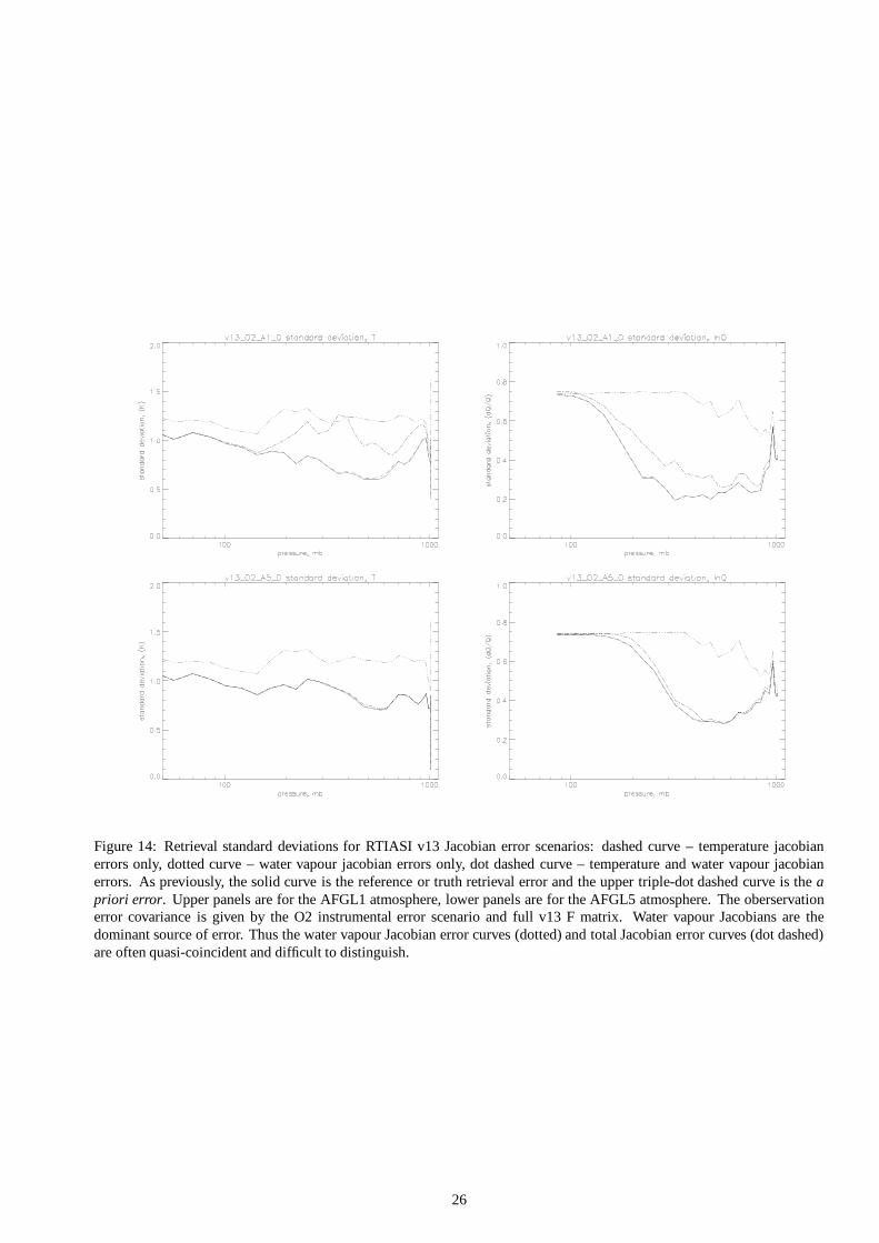
Figure 14: Retrieval standard deviations for RTIASI v13 Jacobian error scenarios: dashed curve – temperature jacobianerrors only, dotted curve – water vapour jacobian errors only, dot dashed curve – temperature and water vapour jacobianerrors. As previously, the solid curve is the reference or truth retrieval error and the upper triple-dot dashed curve is the apriori error. Upper panels are for the AFGL1 atmosphere, lower panels are for the AFGL5 atmosphere. The oberservationerror covariance is given by the O2 instrumental error scenario and full v13 F matrix. Water vapour Jacobians are thedominant source of error. Thus the water vapour Jacobian error curves (dotted) and total Jacobian error curves (dot dashed)are often quasi-coincident and difficult to distinguish.

26

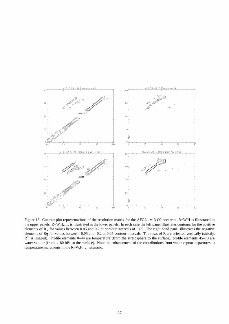
Figure 15: Contour plot representations of the resolution matrix for the AFGL1 v13 O2 scenario. R=W.H is illustrated inthe upper panels, R=W.H � �� is illustrated in the lower panels. In each case the left panel illustrates contours for the positiveelements of R �

�for values between 0.05 and 0.2 at contour intervals of 0.05. The right hand panel illustrates the negative

elements of R ��

for values between -0.05 and -0.2 at 0.05 contour intervals. The rows of R are oriented vertically (strictly,R ) is imaged). Profile elements 0–44 are temperature (from the stratosphere to the surface), profile elements 45–73 arewater vapour (from � 80 hPa to the surface). Note the enhancement of the contributions from water vapour departures totemperature increments in the R=W.H � �� scenario.

27

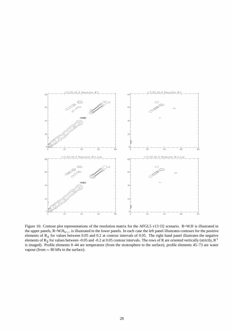
Figure 16: Contour plot representations of the resolution matrix for the AFGL5 v13 O2 scenario. R=W.H is illustrated inthe upper panels, R=W.H � �� is illustrated in the lower panels. In each case the left panel illustrates contours for the positiveelements of R �

�for values between 0.05 and 0.2 at contour intervals of 0.05. The right hand panel illustrates the negative

elements of R ��

for values between -0.05 and -0.2 at 0.05 contour intervals. The rows of R are oriented vertically (strictly, R )is imaged). Profile elements 0–44 are temperature (from the stratosphere to the surface), profile elements 45–73 are watervapour (from � 80 hPa to the surface).

28

Figure 17: Retrieval standard deviations for RTIASI v11 Jacobian error scenarios: dashed curve – temperature jacobian errorsonly, dotted curve – water vapour jacobian errors only, dot dashed curve – temperature and water vapour jacobian errors. Aspreviously, the solid curve is the reference or truth retrieval error and the upper triple-dot dashed curve is the a priori error.Upper panels are for the AFGL1 atmosphere, lower panels are for the AFGL5 atmosphere. The observation error covarianceis given by the O2 instrumental error scenario and full v11 F matrix. Water vapour Jacobians are the dominant source of error.Thus the water vapour Jacobian error curves (dotted) and total Jacobian error curves (dot dashed) are often quasi-coincidentand difficult to distinguish.

29

4 Conclusions and recommendations

Accurate estimates of RTIASI-specific forward model error covariance have been made for two versions of the RTIASImodel, v13 and v11, using three-case and single-case water vapour predictor schemes respectively. Errors present a highdegree of correlation within spectral bands and within the window regions. The only significant difference between the twoschemes occurs in the H � O � � band, where the v11 scheme forward model errors are higher. However, detailed examinationof the errors indicates that the largest degradation occurs for channels which were already relatively poorly modelled in thethree-case water vapour predictor scheme. The error correlation structure also differs quite significantly between the twomodels in the H � O �� band.

The inter-channel correlation structure of instrumental noise is localised spectrally to fourth nearest neighbours. Thuslong-range correlation structure is governed by the forward model error contribution to the observation error covariancematrix. Forward model errors are comparable with revised CNES noise estimates in the 1250 – 1800 cm � interval – theH � O � � band. Accordingly, in this interval forward model error covariance makes a significant contributions to the off-diagonal components of the observation error covariance matrix.

Studies have been undertaken to assess the impact of approximating and/or neglecting forward model error correlationson retrieval accuracy. Where instrumental noise is the dominant term in the observation error covariance, a diagonal (banddiagonal) approximation to the forward model error covariance matrix is adequate. The results of the studies presented heresuggest that for E � � /F � � � 4:1 a diagonal approximation does not introduce significant error in retrievals. The adequacy of adiagonal approximation for spectral intervals where forward model error and instrumental noise are comparable in magnitudeand which are given significant weight in determining analysis increments is less clear. If correlated errors in the H � O � � bandare neglected, temperature and humidity retrievals in the mid and upper troposphere are degraded. In the cases consideredhere this never leads to retrieval errors which are larger than the uncertainty in the a priori estimate of atmospheric state.However, the benefit of the data assimilation process – as measured by the reduction of variance or fraction of unexplainedvariance – can be significantly reduced, particularly in the case of temperature retrievals. In all cases, the degradationof retrieval accuracy is negligible when a block diagonal approximation to the forward model error covariance matrix isassumed in the calculation of the gain matrix.

Spectroscopic uncertainties and representativity errors are expected to give additional correlated errors in the H � O � �

band – this is also true of the CO � and O # bands and the window regions (continuum absorption). Although it is not yet clearwhat the magnitude of these contributions to the observation error covariance (after bias correction) will be, given the currentrelative magnitudes of forward model error and instrumental noise, it would appear that some treatment of error correlation inthe H � O � � band will probably be required. The validity of a (band) diagonal approximation to the error covariance in otherspectral regions will again depend on the magnitude of contributions to the covariance due to spectroscopic uncertaintiesand representativity errors. Even in the revised CNES scenario instrumental errors are the dominant contribution to O: withthe exception of the 750 – 850 cm � interval E � � /F � � � 4:1. Thus one can be reasonably optimistic that a (band) diagonalapproximation will be appropriate for the CO � bands. Treatment of error in the window region will depend on preprocessing– cloud clearing and application of a land/sea mask – and here too a treatment of error correlation may be required.

Discussion has focussed on the specification of the observation error covariance for IASI. If a similar forward model isadopted for AIRS, there is no reason for forward model error characteristics to be substantially modified. The instrumentalnoise characteristics of the AIRS instrument are quite different – noise is uncorrelated from channel to channel, noise levelsare much lower throughout most of the IASI spectral interval5. In this case, forward model errors will be the dominantcomponent of the observation error covariance matrix, and the unique source of correlated error. Retrieval error covarianceestimates have been made for an AIRS noise scenario. As previously, when error correlations are neglected in the H � O � �

band tropospheric temperature and humidity retrievals are degraded by 0.1 – 0.2 K, 5 � in dq/q for the v13 scenario, and0.2 – 0.4 K, 10 � in dq/q for the v11 scenario. Stratospheric temperature retrievals are also slightly degraded ( � 0.1 K)reflecting the influence of error correlation in the CO � bands. In the AFGL tropical atmosphere this increase in retrievalerror corresponds to an approximate doubling in the fraction of unexplained variance in the mid and upper troposphere – thediagonal approximation is a tolerable but distinctly sub-optimal approximation to the forward model error covariance matrix.

Jacobian error estimates have been made for the v11 model, complementing v13 model Jacobians calculated previously.For the two atmospheres considered, the v11 water vapour Jacobians were more accurate than v13 water vapour Jacobians inthe AFGL tropical atmosphere. The inverse is true for the AFGL sub-arctic winter atmosphere. Temperature Jacobians areessentially unmodified in the v11 scheme.

These estimates have been used to quantify the impact of Jacobian errors on retrieval accuracy. The impact of errors intemperature Jacobians on retrieval accuracy is negligible, suggesting a target accuracy of � 5 � for relative errors in fast modelJacobians. Accurate water vapour Jacobians are critical for mid and upper tropospheric temperature and humidity retrievals,and this is the only instance where the adequacy of the RTIASI model is called into question. Errors in the v13 model watervapour Jacobians for the AFGL tropical atmosphere (10 – 40 � errors) give significant degradation in retrieval accuracy, andin some situations degrades the a priori estimate of temperature. The v11 model AFGL1 water vapour Jacobians are moreaccurate than the v13 Jacobians, and the impact of Jacobian errors on retrieval accuracy is reduced by about a factor two.

5AIRS instrumental noise is of the order of 0.05 K (NdTB, 280K scene temperature) throughout the 1000 – 2300 cm �� interval and less than 0.2 Kbetween 2300 and 2700 cm �� . Between 650 and 750 cm �� AIRS noise levels are comparable with the original CNES IASI noise estimates and comparableor less then CNES revised noise estimates between 750 and 1000 cm �� .

30

The v11 performance in the sub-arctic winter case is poorer and the contribution to errors in water vapour retrievals fromJacobian errors is approximately twice that of the AFGL5 v13 case. The impact of Jacobian errors on temperature retrievalaccuracy is small in all cases for the AFGL5 atmosphere.

If the results presented here can be generalised to the range of humid and dry atmospheres encountered in reality, then itwould appear that the v11 RTIASI model with a full or block diagonal forward model error covariance specification is themost appropriate choice of the two RTIASI versions tested. This hypothesis (generalisation of results to a wider range ofatmospheric states) needs to be fully tested, and will require the extension of GENLN2 Jacobian calculations to a wider rangeof states on the full IASI spectral interval. Such an undertaking is computationally demanding, so simulation parameters(e.g. spectral and vertical resolution, magnitudes of parameter perturbations for finite difference Jacobian estimates) shouldbe selected to ensure that these Jacobian calculations may be used as a general reference set.

Improvements to modelled water vapour Jacobians are still necessary, even for the v11 model. Results from VS2000suggest avenues to be explored. Finite difference water vapour Jacobians for the PFAAST model were comparable in accuracywith RTIASI temperature Jacobians. Now, the PFAAST model is based on the same pressure level optical depth formalismas RTIASI, but differs in the detail of its implementation. Four of these implementation differences are susceptible to accountfor differences in modelled water vapour: the profile set used to derive predictor regression coefficients, choice of predictors,separation of absorption contributions from water vapour lines and continuum and model vertical resolution.

In the first instance, an assessment of the impact of the dry bias in the set of profiles used to generate the RTIASItransmittance predictor coefficients on the accuracy of modelled water vapour absorption (Jacobian and forward model errors)should be undertaken, as this would appear a logical source for the errors observed. If this is not a major source of error, thenthe impact of model vertical resolution and the details of the implementation of the predictor scheme should be examined.Should none of these studies give the required improvements, new methods for fast water vapour transmittance calculations(forward and adjoint) will have to be considered.

The results presented here highlight the importance of accurate radiative transfer calculations for the H � O � � band whenundertaking the simultaneous retrieval of temperature and humidity. Based on preliminary intercomparisons of line-by-lineradiative transfer calculations and AERI and HIS measurements undertaken in the framework of the ISSWG line-by-lineintercomparison study (Peter Rayer, private communication) one might expect quite large errors (of the order of Kelvin)in the H � O � � band. Whether due to spectroscopic uncertainities or representativity errors, forward model errors of thismagnitude imply errors in modelled Jacobians of at least the magnitude considered here. Similarly, the nonlinearity ofthe radiative transfer in the H � O �� band (with respect to perturbations of the magnitude of the uncertainty in the a prioriestimate of water vapour concentrations) will give rise to error in modelled Jacobians and estimates of the gain matrix. Theoptimal use of high resolution sounder observations will necessitate improvements to water vapour modelling in the largestsense of the problem (improvements to fast models, improved spectrocopic parameter and improved NWP descriptions ofthe spatio-temporal distribution of water vapour, particularly in the upper troposphere). Indeed, it may be beneficial to makeconservative use of IASI data in a day-one assimilation scheme, through the use of CO � temperature sounding informationonly.

AcknowledgementsI would particularly like to thank Marco Matricardi for providing GENLN2 radiance calculations for the 117 diverse profileset and Andrew Collard, Sean Healy and Clive Rodgers for useful discussions during the course of this work. Many thankstoo to John Eyre and Roger Saunders for pertinant comments on this manuscript.

31

A Error analysis for the gain matrix calculation

We wish to evaluate bounds for errors in analysis increments x due to the the propagation of roundoff error when evaluatingthe gain matrix using Cholesky decomposition. We consider the difference x-x / of the analysis increments x=Wy and x / =W / yin the spectral norm (denoted

� � � ):� �� / � � � � � � � / � � � � � � � / �� (9)

where the inequality follows from the relation

� + � �� + �� +�� (10)

i.e. for a given observation vector y, the spectral norm of x-x / is bounded above by� � � � / �� .

Denoting the innovation error covariance ( � � �� ) � � � ) by the letter I, the gain matrix W can be expressed as:

� � & � � ) � � � (11)

To first order, W - W / is governed by roundoff errors dI and dO in the evaluation of the Cholesky decomposition of I and Orespectively:

� / � �& ��. & � � � ) � � �� / � & � � ) � �-��. � � � � (12)

and

� � � � / � � � & � � ��& �-. & � � �� ) � � � �� / � � � & � � ) �� . � � � � � (13)

In order to evaluate� + � � � +��-./+ � � � for a general square matrix A, we apply the following theorem [7]:

If A is nonsingular and r=� + � ./+ � � � then

� + � � � +�� . + � � � � � ./+ �� + � � � � � � �.� � .Furthermore, application of equation 10 gives the following relation for r: r=

� + � ./+ � � � + � �� . + � . All we require nowis a bound for the spectral norm of the error or perturbation dA.

The Cholesky decomposition of a symmetric positive definite matrix A, LL ) = A + dA has well defined bounds for theerror in the decomposition dA. Kielbasinski [8] derives error bounds for the spectral norm of dA:

� . + � � � � �� % � � � � � � % � � � � � + � � (14)

where � is the rank of A and % � is the unit roundoff error. For large � and small unit roundoff error, Equation 14 can beexpressed as: � ./+ � � % � �� + � � (15)

Using Kielbasinski’s results we find� + � �� ./+ � � % � � �� + � where � �� + � � � + �� + � � is the spectral norm

condition number of A. We apply this last relation to determine wether the criterion r � 1 holds for the innovation andobservation error covariance matrices. Calculations are performed at real8 precision – unit roundoff error is of the order of10 �� . For the innovation matrix n

�=75 and � � �& � is of the order of 10 � – 10 � . Thus for the innovation matrix r

� � 10 �� –10 �� 1. For the observation error covariance matrix n

# � 1000 – 10000 and � � � � � is of the order of 10 � – 10 � . Thusfor the observation error covariance matrix r

# � 10 # – 10 �� . As r � 1 in both cases, the theorem above may be applied todetermine the bounds for

� � � � / � :� � � � / � � % � � � �& � � � �� & � �� ) �� /� � ��

� � � �� ) �� / � � % � � � � � � � ��# � & � �� ) �� /� � �.� # �

� � � # �� ) �� (16)

The bound for errors due to errors in the Cholesky decomposition of the observation error covariance matrix are � 10 � timesgreater than the corresponding bound for errors in the innovation matrix. The magnitude of these errors can be reduced byimproving the condition of the observation error covariance matrix through choice of metric and by reducing the dimensionof the observation error covariance matrix through channel selection. For example for the NdTb metric and the 1057 channelsampling

� � � � / � �� /�� & � �� ) �� . Finally, note that in absolute terms these errors are small, smaller than thecorresponding norms for the approximations to the forward model error covariance matrix for example: with real8 precisionroundoff errors are a negligible source of error in the calculations presented here.

32

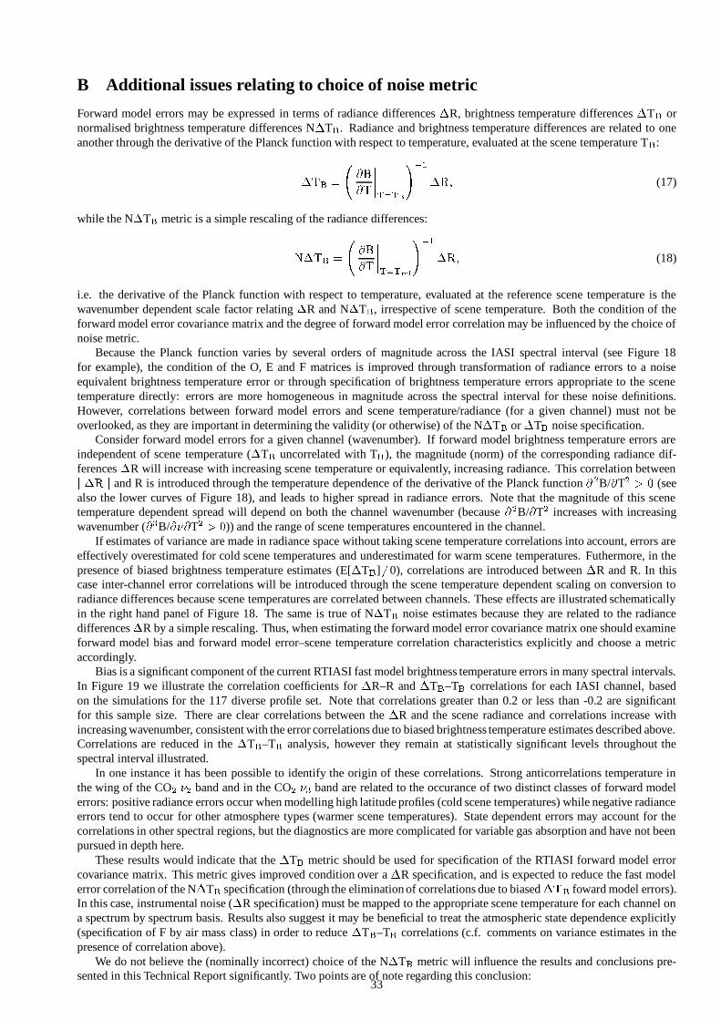
B Additional issues relating to choice of noise metric

Forward model errors may be expressed in terms of radiance differences � R, brightness temperature differences � T�

ornormalised brightness temperature differences N � T

�. Radiance and brightness temperature differences are related to one

another through the derivative of the Planck function with respect to temperature, evaluated at the scene temperature T�

:

�� )�� )�� (17)

while the N � T�

metric is a simple rescaling of the radiance differences: � �� )�� )�� (18)

i.e. the derivative of the Planck function with respect to temperature, evaluated at the reference scene temperature is thewavenumber dependent scale factor relating � R and N � T

�, irrespective of scene temperature. Both the condition of the

forward model error covariance matrix and the degree of forward model error correlation may be influenced by the choice ofnoise metric.

Because the Planck function varies by several orders of magnitude across the IASI spectral interval (see Figure 18for example), the condition of the O, E and F matrices is improved through transformation of radiance errors to a noiseequivalent brightness temperature error or through specification of brightness temperature errors appropriate to the scenetemperature directly: errors are more homogeneous in magnitude across the spectral interval for these noise definitions.However, correlations between forward model errors and scene temperature/radiance (for a given channel) must not beoverlooked, as they are important in determining the validity (or otherwise) of the N � T

�or � T

�noise specification.

Consider forward model errors for a given channel (wavenumber). If forward model brightness temperature errors areindependent of scene temperature ( � T

�uncorrelated with T

�), the magnitude (norm) of the corresponding radiance dif-

ferences � R will increase with increasing scene temperature or equivalently, increasing radiance. This correlation between��

and R is introduced through the temperature dependence of the derivative of the Planck function� � B/

�T � � � (see

also the lower curves of Figure 18), and leads to higher spread in radiance errors. Note that the magnitude of this scenetemperature dependent spread will depend on both the channel wavenumber (because

� � B/�

T � increases with increasingwavenumber (

� # B/��

T � �� )) and the range of scene temperatures encountered in the channel.If estimates of variance are made in radiance space without taking scene temperature correlations into account, errors are

effectively overestimated for cold scene temperatures and underestimated for warm scene temperatures. Futhermore, in thepresence of biased brightness temperature estimates (E[ � T

�] �� 0), correlations are introduced between � R and R. In this

case inter-channel error correlations will be introduced through the scene temperature dependent scaling on conversion toradiance differences because scene temperatures are correlated between channels. These effects are illustrated schematicallyin the right hand panel of Figure 18. The same is true of N � T

�noise estimates because they are related to the radiance

differences � R by a simple rescaling. Thus, when estimating the forward model error covariance matrix one should examineforward model bias and forward model error–scene temperature correlation characteristics explicitly and choose a metricaccordingly.

Bias is a significant component of the current RTIASI fast model brightness temperature errors in many spectral intervals.In Figure 19 we illustrate the correlation coefficients for � R–R and � T

�–T

�correlations for each IASI channel, based

on the simulations for the 117 diverse profile set. Note that correlations greater than 0.2 or less than -0.2 are significantfor this sample size. There are clear correlations between the � R and the scene radiance and correlations increase withincreasing wavenumber, consistent with the error correlations due to biased brightness temperature estimates described above.Correlations are reduced in the � T

�–T

�analysis, however they remain at statistically significant levels throughout the

spectral interval illustrated.In one instance it has been possible to identify the origin of these correlations. Strong anticorrelations temperature in

the wing of the CO � � � band and in the CO � � # band are related to the occurance of two distinct classes of forward modelerrors: positive radiance errors occur when modelling high latitude profiles (cold scene temperatures) while negative radianceerrors tend to occur for other atmosphere types (warmer scene temperatures). State dependent errors may account for thecorrelations in other spectral regions, but the diagnostics are more complicated for variable gas absorption and have not beenpursued in depth here.

These results would indicate that the � T�

metric should be used for specification of the RTIASI forward model errorcovariance matrix. This metric gives improved condition over a � R specification, and is expected to reduce the fast modelerror correlation of the N � T

�specification (through the elimination of correlations due to biased �

� �foward model errors).

In this case, instrumental noise ( � R specification) must be mapped to the appropriate scene temperature for each channel ona spectrum by spectrum basis. Results also suggest it may be beneficial to treat the atmospheric state dependence explicitly(specification of F by air mass class) in order to reduce � T

�–T

�correlations (c.f. comments on variance estimates in the

presence of correlation above).We do not believe the (nominally incorrect) choice of the N � T

�metric will influence the results and conclusions pre-

sented in this Technical Report significantly. Two points are of note regarding this conclusion:33

(i) As described above, forward model errors tend to be overestimated at cold scene temperatures and underestimated atwarm scene temperature. This implies that slightly more weight should be give to the observations in the AFGL5 case, andslightly less weight should be give to the observations in the AFGL1 case. This in turn would tend to increase errors (small)due to approximations to F or Jacobian errors in the AFGL5 case and decrease them in the AFGL1 case. The AFGL1 casesillustrated can therefore be interpreted in terms of an upper bound.(ii) The presence relatively strong � T

�–T

�correlations observed would tend to suggest N � T

�error covariance estimates

are not unrealistic: as noted above, error correlations of this type will give rise to inter-channel forward model error correla-tions and are undoubtably a significant component of the error covariance estimates for the current RTIASI model (correlationcharacteristics were not significantly reduced on passage from the � R to the � T

�metric, illustrated in Figure 19).

34

T=200 K

T=250 K

T=300 K

Planck function B(T) for

1e-08

1e-07

1e-06

1e-05

0.0001

0.001

0.01

0.1

1

1000 1500 2000 2500

wavenumber

dT

dB

T=T*

TB

TB

TB

δBδT T2δB

δT T1

δBδT T2

TB

TB

TB

δBδT T1

0

d

σ

T1 T2

R

R

d

σR

0

Biased uncorrelated dT BUnbiased uncorrelated dT B

d

σ

T1 T2

R

R

d

σR0

Figure 18: Left hand panel: spectral and temperature dependencies of the Planck function, B(T) [W/sr/m � /cm � ] and thederivative of the Planck function

� � � �� [W/sr/m � /cm � /K] evaluated at the scene temperatures (T�

) for three characteristicatmospheric scene temperatures (300, 250 and 200 K). Note

� � � � �� increases with increasing wavenumber. Right handpanel: schematic illustration of the introduction of scene-radiance dependent spread in radiance errors and the introduc-tion of correlation with scene radiance due to biased forward model brightness temperature errors through the temperaturedependence of the Planck function derivative

� � � �� .

-1

-0.8

-0.6

-0.4

-0.2

0

0.2

0.4

0.6

0.8

1

500 1000 1500 2000 2500 3000

corr

elat

ion

coef

ficie

nt

wavenumber

Correlation between radiance errors and scene radiance

-1

-0.8

-0.6

-0.4

-0.2

0

0.2

0.4

0.6

0.8

1

500 1000 1500 2000 2500 3000

corr

elat

ion

coef

ficie

nt

wavenumber

Correlation between brightness temperature errors and scene temperature

Figure 19: Correlation coefficients for � R–R and � T�

–T�

correlations for each IASI channel (left and right hand panelsrespectively), based on the simulations for the 117 diverse profile set. Correlations greater than 0.2 or less than -0.2 aresignificant for this sample size. Correlations are reduced for the � T

�metric, but remain at statistically significant levels for

most of the IASI spectral interval.

35

References

[1] V. J. Sherlock. Results from the first UKMO IASI fast radiative transfer model intercomparison. Technical ReportFR-287, The Met. Office, Bracknell, United Kingdom, 2000.

[2] Technical Report IATN-0000-5479-CNE, Centre Nationale d’Etudes Spatiales, Toulouse, France, 1996.

[3] F. Cayla. Communication to ISSWG, Aix-en-Provence, 1999. Report available from P. Schlussel, EUMETSAT.

[4] U. Amato, D. de Canditiis, and C. Serio. Effect of apodisation on the retrieval of geophysical parameters from FourierTransform spectrometers. Appl. Optics, 37(27):6537–6543, 1999.

[5] C. D. Barnet and J. Susskind. Simulation studies of advanced infrared and microwave sounders. In Proceedings of theTenth International TOVS Study Conference, Boulder CO, 1999.

[6] R. O. Weber and P. Talkner. Some remarks on spatial correlation function models. Monthly Weather Rev., 121:2611–2617, 1993.

[7] G. H. Golub and C. F. Van Loan. Matrix computations. John Hopkins University Press, 1996.

[8] A. Kielbasinski. A note on the rounding error analysis of Cholesky factorisation. Linear Algebra and its Applications,88/89:487–494, 1987.

[9] F. Chevallier. Sampled databases of atmopsheric profiles from the ECMWF 50-level forecast model. Technical report,European Centre for Medium-range Weather Forecasts, Reading, United Kingdom, 1999.

[10] A. D. Collard. The effect on undetected cloud on IASI retrievals. Technical Report FR-261, The Met. Office, 1999.

[11] P. D. Watts and A. P. McNally. The sensitivity of a minimum variance retrieval scheme to the value of its principalparameters. In Proceedings of the Fourth International TOVS Study Conference; Igls, Austria; 16-22 March, 1988.CIMSS, Univ. Wisconsin, Madison, 1988.

[12] C. D. Rodgers. Characterisation and error analysis of profiles retrieved from remote sounding measurements. J. Geo.Res., 95(D5):5587–5595, 1990.

[13] C. D. Rodgers. Information content and optimisation of high spectral resolution measurements. SPIE 2830, Opticalspectroscopic techniques and instrumentation for atmospheric and space research II, pages 136–147, 1996.

[14] J. R. Eyre. The effects of non-linearity on analysis and retrieval errors. Technical Report FR-252, The Met. Office,1998.

[15] J. Eyre and A. Collard. The effects of nonlinearity on retrieval errors: implications for the interpretation of advancedIR sounder data. In Proceedings of the Tenth International TOVS Study Conference, Boulder CO, USA, pages 191–202,1999.

[16] H.L. Huang, W. L. Smith, and H. M. Woolf. Vertical resolution and accuracy of atmopsheric infrared sounding inter-ferometers. J. Appl. Meteorol., pages 265–274, 1992.

[17] A. D. Collard. Notes on IASI performance. Technical Report FR-256, The Met. Office, Bracknell, United Kingdom,1998.

[18] G. E. Backus and J. F. Gilbert. Uniqueness in the inversion of inaccurate gross Earth data. Philos. Trans. R. Soc.London, Ser. A, 266:123–192, 1970.

36

Impact of RTIASI fast radiative transfer model error on ... · This study quantiﬁes the impact of...

Documents

Transcript of Impact of RTIASI fast radiative transfer model error on ... · This study quantiﬁes the impact of...