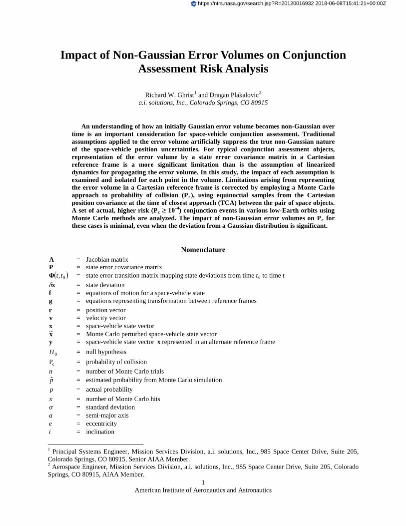
American Institute of Aeronautics and Astronautics

1

Impact of Non-Gaussian Error Volumes on Conjunction Assessment Risk Analysis

Richard W. Ghrist1 and Dragan Plakalovic2

a.i. solutions, Inc., Colorado Springs, CO 80915

An understanding of how an initially Gaussian error volume becomes non-Gaussian over time is an important consideration for space-vehicle conjunction assessment. Traditional assumptions applied to the error volume artificially suppress the true non-Gaussian nature of the space-vehicle position uncertainties. For typical conjunction assessment objects, representation of the error volume by a state error covariance matrix in a Cartesian reference frame is a more significant limitation than is the assumption of linearized dynamics for propagating the error volume. In this study, the impact of each assumption is examined and isolated for each point in the volume. Limitations arising from representing the error volume in a Cartesian reference frame is corrected by employing a Monte Carlo approach to probability of collision (Pc), using equinoctial samples from the Cartesian position covariance at the time of closest approach (TCA) between the pair of space objects. A set of actual, higher risk (Pc ≥ 10–4) conjunction events in various low-Earth orbits using Monte Carlo methods are analyzed. The impact of non-Gaussian error volumes on Pc

Nomenclature

for these cases is minimal, even when the deviation from a Gaussian distribution is significant.

A = Jacobian matrix P = state error covariance matrix ( )0, ttΦ = state error transition matrix mapping state deviations from time t0

xδ to time t

= state deviation f = equations of motion for a space-vehicle state g = equations representing transformation between reference frames r = position vector v = velocity vector x = space-vehicle state vector x~ = Monte Carlo perturbed space-vehicle state vector y = space-vehicle state vector x represented in an alternate reference frame

0H = null hypothesis

cP = probability of collision n = number of Monte Carlo trials p = estimated probability from Monte Carlo simulation p = actual probability x = number of Monte Carlo hits σ = standard deviation a = semi-major axis e = eccentricity i = inclination

1 Principal Systems Engineer, Mission Services Division, a.i. solutions, Inc., 985 Space Center Drive, Suite 205, Colorado Springs, CO 80915, Senior AIAA Member. 2 Aerospace Engineer, Mission Services Division, a.i. solutions, Inc., 985 Space Center Drive, Suite 205, Colorado Springs, CO 80915, AIAA Member.

https://ntrs.nasa.gov/search.jsp?R=20120016932 2018-06-08T15:41:21+00:00Z

American Institute of Aeronautics and Astronautics

2

Ω = right ascension of the ascending node ω = argument of perigee ν = true anomaly NTW = Normal, in-track, cross-track Cartesian coordinates centered on space-vehicle xyz = Encounter frame coordinates ( x in direction of relative position, y in direction of relative velocity)

Vectors are indicated by bold, lower-case symbols. Matrices are indicated by bold, upper-case symbols. ( )xx dtd≡ ;

ˆ ≡x unit vector of x ; ≡Tx transpose of x ; ⋅E is the expectation operator; I is the identity matrix.

I. Introduction ONJUNCTION assessment risk analysis (CARA) is the process of monitoring and evulating the collision risk from unique close approach events between two space objects. The “big sky” theory, in which it is presumed

that object densities are small enough that the likelihood of collisions between spacecraft is discountable, is no longer valid as evidenced by recent collisions.1

Collision risk can be expressed in several ways, most commonly by the miss distance (the closest in position the two objects will come) or, better, by the probability of collision (P

Satellite protection is critical both to maintain the satellite mission and to avoid polluting the orbital neighborhood.

c). The Pc metric is a useful mechanism to encapsulate risk but it requires accurate knowledge of the state uncertainty, typically represented by the state error covariance matrix. The analytic calculations of Pc rely on an assumption that the propagated state error distribution is Gaussian.2 This Gaussian assumption appears to be on questionable ground, and the impact of this non-Gaussian behavior on Pc is not well understood.3 The orbit determination process results in an initially Gaussian error distribution, generally assuming that the observation residuals are independent and identically distributed from a zero-mean Gaussian and the dynamics are suitably modeled. In practice, however, these assumptions may not be entirely true. Assuming an initially Gaussian error volume, longer-term non-Gaussian behavior in the error volume often becomes evident after a couple of days of propagation, even for well-tracked objects.4 Operations for the National Aeronautics and Space Administration (NASA) Robotic CARA task regularly require predictions a week or more in the future to determine potential conjunction assessment events of interest. Therefore, a significant deviation from a Gaussian error volume may be expected. Prior to developing a solution to mitigate or fix non-Gaussian effects, this investigation addresses the nature of non-Gaussian effects from propagation for low-Earth orbit (LEO) objects and, subsequently, determines the resulting impact to Pc

II. Background on Non-Gaussian Error Volumes

using a Monte Carlo approach on a set of actual, high risk events from the NASA Robotic CARA task.

An initially Gaussian error volume representing space-vehicle uncertainties will become non-Gaussian over time, which is a consequence of the nonlinear dynamics governing space-vehicle motion. This nonlinearity is a fundamental aspect of the dynamical system and its coordinate system representation.5

This section first reviews how the true non-Gaussian nature of the error volume is artificially suppressed by using a linearized dynamical system to propagate the error volume (linearized dynamics) and by representing the error volume in a Cartesian reference frame. Then, there is a discussion of methods to recover, in part or in whole, the true non-Gaussian nature of the error volume. Finally, there is a review of research that relates non-Gaussian error volumes to conjunction assessment.

To correctly process how an initial Gaussian error volume evolves over time, nonlinear dynamics must be utilized. The effects from the nonlinear dynamics on the error volumes becomes more evident for larger initial error volumes and for longer propagation times.

A. Source of Evolution to Non-Gaussian Error Volumes The state error covariance matrix P is routinely used to represent the uncertainty of a satellite state vector x in

terms of a Gaussian ellipsoid. This covariance may not match the true state uncertainty; if they do agree, Horwood et al.6 refer to this condition as uncertainty consistency. In Junkins et al.,7

C

an investigation of how an initially Gaussian error volume becomes non-Gaussian over time is presented. In that research, they present two aspects where linearization assumptions with regard to how the error volume is handled can suppress the true non-Gaussian nature of the error volume. The first aspect relates to the assumption of linearized dynamics in error theory, as the entire error volume is propagated based on a linearized Jacobian evaluated at the nominal state (refer to the Appendix for

American Institute of Aeronautics and Astronautics

3

additional information). The linearized dynamics assumption is summarized by the similarity transformation for propagating covariance from one time t0

to another time t using the state error transition matrix, Φ, that is,

( ) ( ) ( ) ( )000 ,, tttttt TΦPΦP = . (1)

The second aspect where a linearization of the error volume appears is with transformations between reference frames. If one frame x relates to another frame y by

( )xgy = , (2)

then the covariance in frame x can be transformed to frame y using a similarity transformation, that is,

TAAPP xy = , (3)

where

∂∂

=xgA (4)

is the linearized Jacobian evaluated at the nominal state. A Cartesian representation for the covariance, as is used for current CARA operations, is an unfortunate choice

for representing the error volume of a nonlinear trajectory. Similarity transformations for covariance, by their nature, are shape-preserving, so an initially Gaussian error volume will artificially remain Gaussian for all time and in any reference frame. If the error volume becomes too large, whether due to a long propagation time, a large initial uncertainty volume, or some combination of the two, then these linearization assumptions can result in the covariance being an inadequate representation of the actual uncertainty volume – a violation of uncertainty consistency. The non-Gaussian effects can become evident on a timescale of hours to days. This situation is most challenging when dealing with uncorrelated target (UCT) initial orbit determination (IOD) objects, as the initial uncertainty volumes are large and problematically-shaped, but non-Gaussian error volumes must be considered for conjunction assessment activities as well.

B. Techniques to Recover the Non-Gaussian Error Volume Methods for restoring the true non-Gaussian state error distribution can be classified into several categories. The

first is the familiar Monte Carlo strategy. The second involves the selection of an alternative coordinate representation for the error volume to address the limitations of the Cartesian reference frame, and the third addresses the linearized dynamics assumption for propagating the error volume.

The Monte Carlo method, taking pseudo-random Gaussian perturbations of the state uncertainty at epoch and propagating these perturbed states, is an accurate representation of the error volume and is often employed as a truth source for the propagated uncertainty state. In representing the error uncertainty as a cloud of points that are propagated with the full nonlinear dynamics, there are no linearization assumptions involved. Monte Carlo methods can come with a severe computational cost as all perturbed states must be propagated, which has been a motivational factor to formulate alternative approaches.

Another technique to recover the non-Gaussian error volume is to select an alternative set of coordinates in which the covariance more closely approximates the true error volume. One approach is to change the coordinates used for propagating the covariance, such as classical orbit elements,8 equinoctial orbit elements,4,7,9,10 Poincaré orbit elements,11,12 polar coordinates,7 and curvilinear coordinates.4,13,14 Another approach is to simply transform the Cartesian covariance into a more suitable representation using Eq. (3) at the end of the propagation time. Sabol et al.4

Addressing the linearized dynamics assumption for propagating the error volume is challenging as this assumption relates to how the state uncertainty is propagated. One approach is to replace the linearized dynamics for propagating the error volume with a higher order error theory, generalizing the state error transition matrix as a state

demonstrate this method by transforming the covariance from osculating Cartesian Earth-centered inertial (ECI) into osculating equinoctial. Both approaches to this technique are computationally efficient, as only a single state vector and the associated covariance matrix are propagated.

American Institute of Aeronautics and Astronautics

4

error transition tensor.11,15,16 Another approach employing Gaussian mixture models17 addresses the limitations of representing the error volume as a single Gaussian probability density function (pdf). Gaussian sum filters estimate any arbitrary pdf as a weighted sum of Gaussian components and have been successfully applied to determining satellite error volumes.10,18,19 An added benefit is that Gaussian sum filters may make use of existing uncertainty mapping techniques, such as those employed by extended Kalman filters or unscented Kalman filters, for propagating the Gaussian error volume components. One can also represent the error volume pdf with other formulations, as demonstrated by Edgeworth filters6 and polynomial chaos expansions.12

Techniques that alter the coordinate representation for the error volume and address the linearized dynamics assumption for propagating the error volume are at times intertwined. Junkins et al.

This collection of methods shows potential and could be competitive or superior to a Monte Carlo approach.

7 found that an equinoctial formulation and propagation of covariance performed better than polar coordinate formulation, which in turn performed better than Cartesian coordinate formulation, although the authors did not separate the two sources of nonlinearity. Sabol et al.4 separate the impact of linearized dynamics from the Cartesian comparison frame in their seminal work. Hoots8 maintains that an approximate formulation for the error volume, represented analytically as a polynomial expansion in classical elements, eliminates nonlinearities in both the coordinates and in the propagation of the error volume. Folcik et al.9 claim that mean equinoctial propagation of covariance performs better than osculating equinoctial propagation in containing the truth state. Even a subtle change, replacing the semi-major axis by the mean motion in equinoctial orbit elements, can result in better agreement with the true error volume.

C. Non-Gaussian Effects and Conjunction Assessment

10

While the theory of mitigating non-Gaussian error volumes is relatively mature, the impact of non-Gaussian error volumes to conjunction assessment is not well-characterized at present. Tanygin and Coppola20 assess the impact of the bias term from a second-order error volume propagation on an entire space object catalogue with synthetic covariance values. They examine differences in time of closest approach (TCA), miss distance, and maximum Pc

In their work, Sabol et al.

associated with conjunction events and conclude that this second order bias effect can be significant, e.g., for an object about to decay. The second order bias addresses only one aspect of the impact of non-Gaussian error volumes, as an underlying Gaussian assumption remains and no attempt is made to address the limitations of representing the error volume in Cartesian coordinates.

21 examine the impact of non-Gaussian error volumes on the miss distance distribution. In their Monte Carlo framework, they perform perturbations of the initial covariance matrix and compare the results with both the standard analytic formulation and with Monte Carlo perturbations taken at TCA. Their analysis reveals differences in the distribution of miss distances that are attributable to non-Gaussian error volumes. However, they make no attempt to demonstrate resulting changes in Pc. The Pc metric is the integral of the miss distance pdf with limits of integration from zero up to the combined physical size of the objects. Therefore, the only changes in the miss distance distribution that are significant to Pc are those corresponding to small miss distances. Understanding the impact to Pc

III. Propagated Error Volume Investigations

from non-Gaussian error volumes is the most fundamental aspect from a CARA perspective and is the objective of this study.

Prior to investigating the impact of a non-Gaussian error volume on conjunction assessment events, this section explores the propagation of an initially Gaussian error volume by considering both propagated Monte Carlo samples and the propagated covariance. Then follows a discussion of representing the propagated error volume as equinoctial samples of the propagated Cartesian covariance, which is a mechanism to address the limitations of the Cartesian reference frame. Finally, the errors associated with the assumption of linearized dynamics for propagating the error volume are isolated and found to be negligible for typical conjunction assessment objects.

A. Position Uncertainty Misalignment Angle For the initial investigation into propagated error volumes, the time evolution of an initially Gaussian error volume for a single object in a LEO orbit is considered for objects ranging from 400 km to 1300 km in altitude. A high-fidelity model in FreeFlyer® software is used in the propagation of the nominal and perturbed state vectors; the nominal covariance is propagated numerically using the FreeFlyer® state error transition matrix function. These Monte Carlo perturbations are generated at the initial epoch and represent the true error volume when propagated forward in time. It is instructive to go through one example in detail as its results are representative of the other scenarios. The initial Keplerian state a, e, i, Ω, ω, ν is 7718.4 km, 0.00039, 66.0°, 282.7°, 100.5°, 52.1° and the initial ECI

American Institute of Aeronautics and Astronautics

5

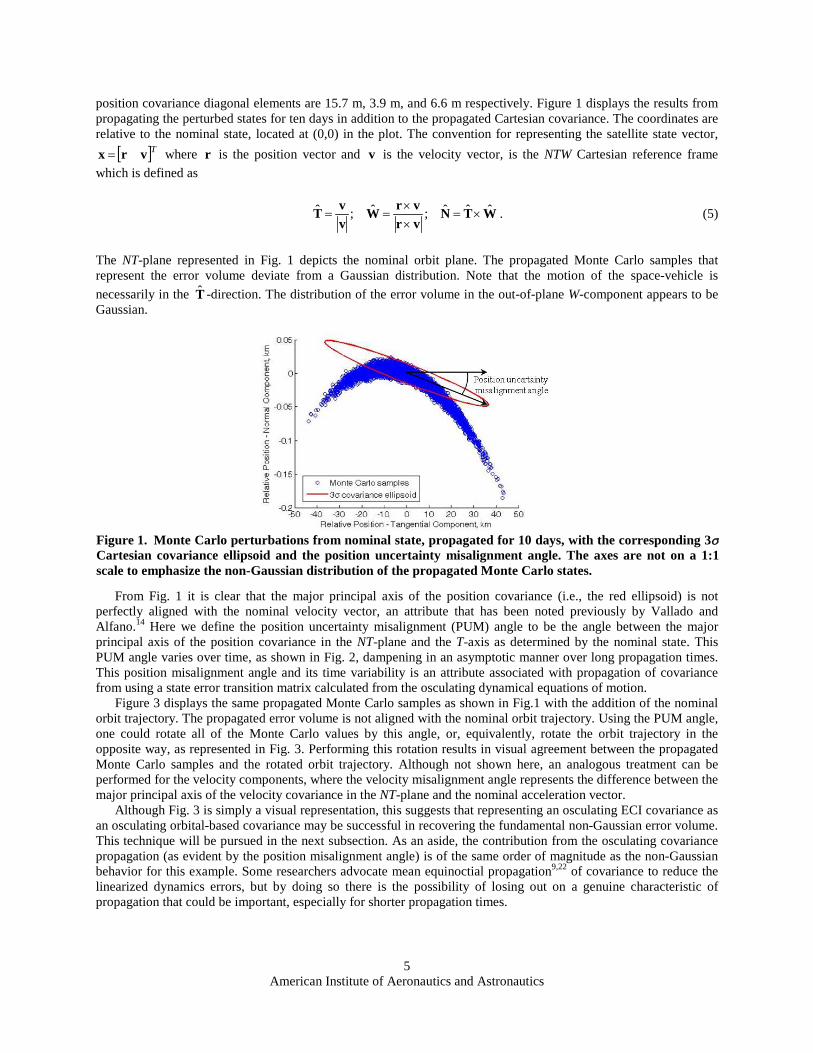
position covariance diagonal elements are 15.7 m, 3.9 m, and 6.6 m respectively. Figure 1 displays the results from propagating the perturbed states for ten days in addition to the propagated Cartesian covariance. The coordinates are relative to the nominal state, located at (0,0) in the plot. The convention for representing the satellite state vector,

[ ]Tvrx = where r is the position vector and v is the velocity vector, is the NTW Cartesian reference frame which is defined as

WTN

vrvrW

vvT ˆˆˆ;ˆ;ˆ ×=

××

== . (5)

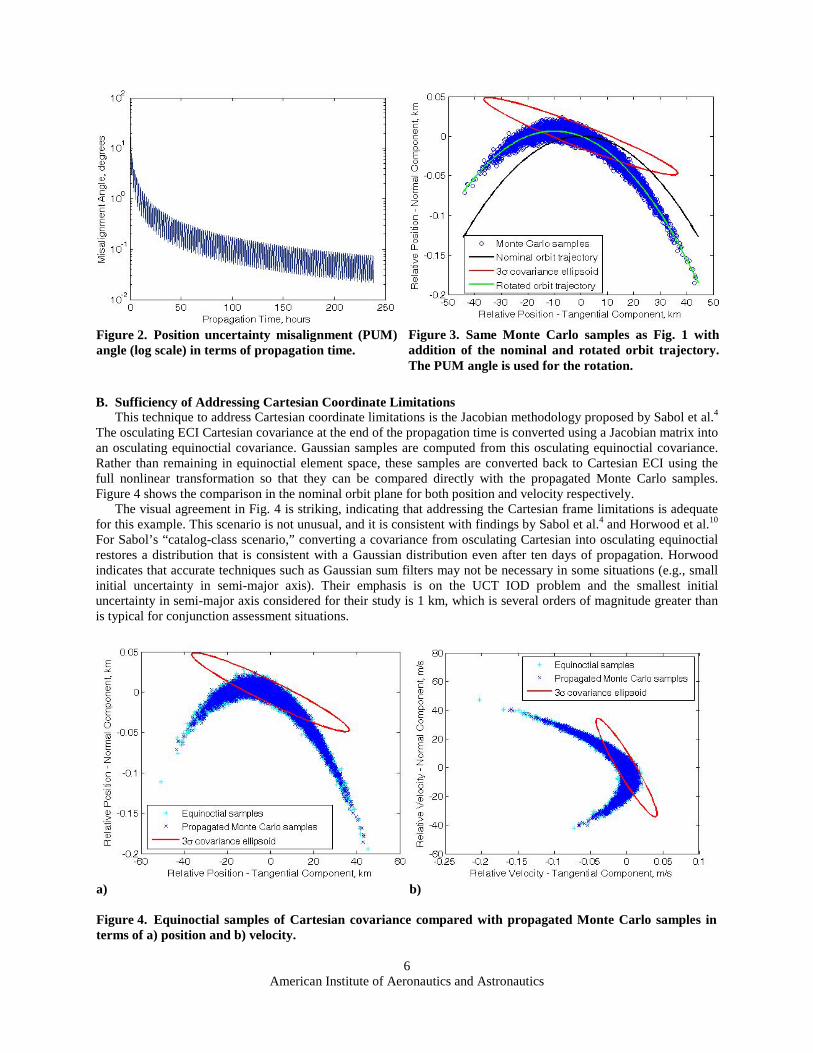
The NT-plane represented in Fig. 1 depicts the nominal orbit plane. The propagated Monte Carlo samples that represent the error volume deviate from a Gaussian distribution. Note that the motion of the space-vehicle is necessarily in the T -direction. The distribution of the error volume in the out-of-plane W-component appears to be Gaussian.

From Fig. 1 it is clear that the major principal axis of the position covariance (i.e., the red ellipsoid) is not perfectly aligned with the nominal velocity vector, an attribute that has been noted previously by Vallado and Alfano.14

Figure 3 displays the same propagated Monte Carlo samples as shown in Fig.1 with the addition of the nominal orbit trajectory. The propagated error volume is not aligned with the nominal orbit trajectory. Using the PUM angle, one could rotate all of the Monte Carlo values by this angle, or, equivalently, rotate the orbit trajectory in the opposite way, as represented in Fig. 3. Performing this rotation results in visual agreement between the propagated Monte Carlo samples and the rotated orbit trajectory. Although not shown here, an analogous treatment can be performed for the velocity components, where the velocity misalignment angle represents the difference between the major principal axis of the velocity covariance in the NT-plane and the nominal acceleration vector.

Here we define the position uncertainty misalignment (PUM) angle to be the angle between the major principal axis of the position covariance in the NT-plane and the T-axis as determined by the nominal state. This PUM angle varies over time, as shown in Fig. 2, dampening in an asymptotic manner over long propagation times. This position misalignment angle and its time variability is an attribute associated with propagation of covariance from using a state error transition matrix calculated from the osculating dynamical equations of motion.

Although Fig. 3 is simply a visual representation, this suggests that representing an osculating ECI covariance as an osculating orbital-based covariance may be successful in recovering the fundamental non-Gaussian error volume. This technique will be pursued in the next subsection. As an aside, the contribution from the osculating covariance propagation (as evident by the position misalignment angle) is of the same order of magnitude as the non-Gaussian behavior for this example. Some researchers advocate mean equinoctial propagation9,22

of covariance to reduce the linearized dynamics errors, but by doing so there is the possibility of losing out on a genuine characteristic of propagation that could be important, especially for shorter propagation times.

Figure 1. Monte Carlo perturbations from nominal state, propagated for 10 days, with the corresponding 3σ Cartesian covariance ellipsoid and the position uncertainty misalignment angle. The axes are not on a 1:1 scale to emphasize the non-Gaussian distribution of the propagated Monte Carlo states.

American Institute of Aeronautics and Astronautics

6

B. Sufficiency of Addressing Cartesian Coordinate Limitations This technique to address Cartesian coordinate limitations is the Jacobian methodology proposed by Sabol et al.4

The visual agreement in Fig. 4 is striking, indicating that addressing the Cartesian frame limitations is adequate for this example. This scenario is not unusual, and it is consistent with findings by Sabol et al.

The osculating ECI Cartesian covariance at the end of the propagation time is converted using a Jacobian matrix into an osculating equinoctial covariance. Gaussian samples are computed from this osculating equinoctial covariance. Rather than remaining in equinoctial element space, these samples are converted back to Cartesian ECI using the full nonlinear transformation so that they can be compared directly with the propagated Monte Carlo samples. Figure 4 shows the comparison in the nominal orbit plane for both position and velocity respectively.

4 and Horwood et al.10 For Sabol’s “catalog-class scenario,” converting a covariance from osculating Cartesian into osculating equinoctial restores a distribution that is consistent with a Gaussian distribution even after ten days of propagation. Horwood indicates that accurate techniques such as Gaussian sum filters may not be necessary in some situations (e.g., small initial uncertainty in semi-major axis). Their emphasis is on the UCT IOD problem and the smallest initial uncertainty in semi-major axis considered for their study is 1 km, which is several orders of magnitude greater than is typical for conjunction assessment situations.

Figure 2. Position uncertainty misalignment (PUM) angle (log scale) in terms of propagation time.

Figure 3. Same Monte Carlo samples as Fig. 1 with addition of the nominal and rotated orbit trajectory. The PUM angle is used for the rotation.

a) b) Figure 4. Equinoctial samples of Cartesian covariance compared with propagated Monte Carlo samples in terms of a) position and b) velocity.

American Institute of Aeronautics and Astronautics

7

C. Isolation of Linearized Dynamics Errors As the technique in the previous subsection only addresses the limitations of the Cartesian coordinate

representation, the purpose of this subsection is to attempt to isolate the other error source: the linearized dynamics errors. Instead of comparing entire distributions (such as by the expected Mahalanobis distance distribution4

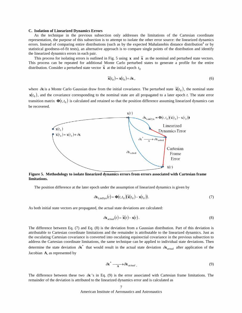
This process for isolating errors is outlined in Fig. 5 using

or by statistical goodness-of-fit tests), an alternative approach is to compare single points of the distribution and identify the linearized dynamics errors in each pair.

x and x~ as the nominal and perturbed state vectors. This process can be repeated for additional Monte Carlo perturbed states to generate a profile for the entire distribution. Consider a perturbed state vector x~ at the initial epoch 0t

( ) ( ) xxx δ+= 00

~ tt , (6)

where xδ is a Monte Carlo Gaussian draw from the initial covariance. The perturbed state ( )0~ tx , the nominal state

( )0tx , and the covariance corresponding to the nominal state are all propagated to a later epoch t. The state error transition matrix ( )0, ttΦ is calculated and retained so that the position difference assuming linearized dynamics can be recovered.

The position difference at the later epoch under the assumption of linearized dynamics is given by

( ) ( ) ( ) ( )( )000LinDyn

~, ttttt xxΦx −=δ . (7)

As both initial state vectors are propagated, the actual state deviations are calculated:

( ) ( ) ( )ttt xxx −= ~

actualδ . (8)

The difference between Eq. (7) and Eq. (8) is the deviation from a Gaussian distribution. Part of this deviation is attributable to Cartesian coordinate limitations and the remainder is attributable to the linearized dynamics. Just as the osculating Cartesian covariance is converted into osculating equinoctial covariance in the previous subsection to address the Cartesian coordinate limitations, the same technique can be applied to individual state deviations. Then determine the state deviation *xδ that would result in the actual state deviation actualxδ after application of the Jacobian ,A as represented by

actualxx A δδ →*. (9)

The difference between these two xδ ’s in Eq. (9) is the error associated with Cartesian frame limitations. The remainder of the deviation is attributed to the linearized dynamics error and is calculated as

Figure 5. Methodology to isolate linearized dynamics errors from errors associated with Cartesian frame limitations.

American Institute of Aeronautics and Astronautics

8

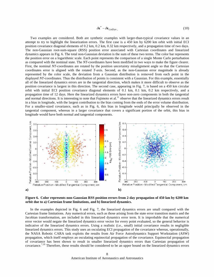
LinDyn* xx δδ − . (10)

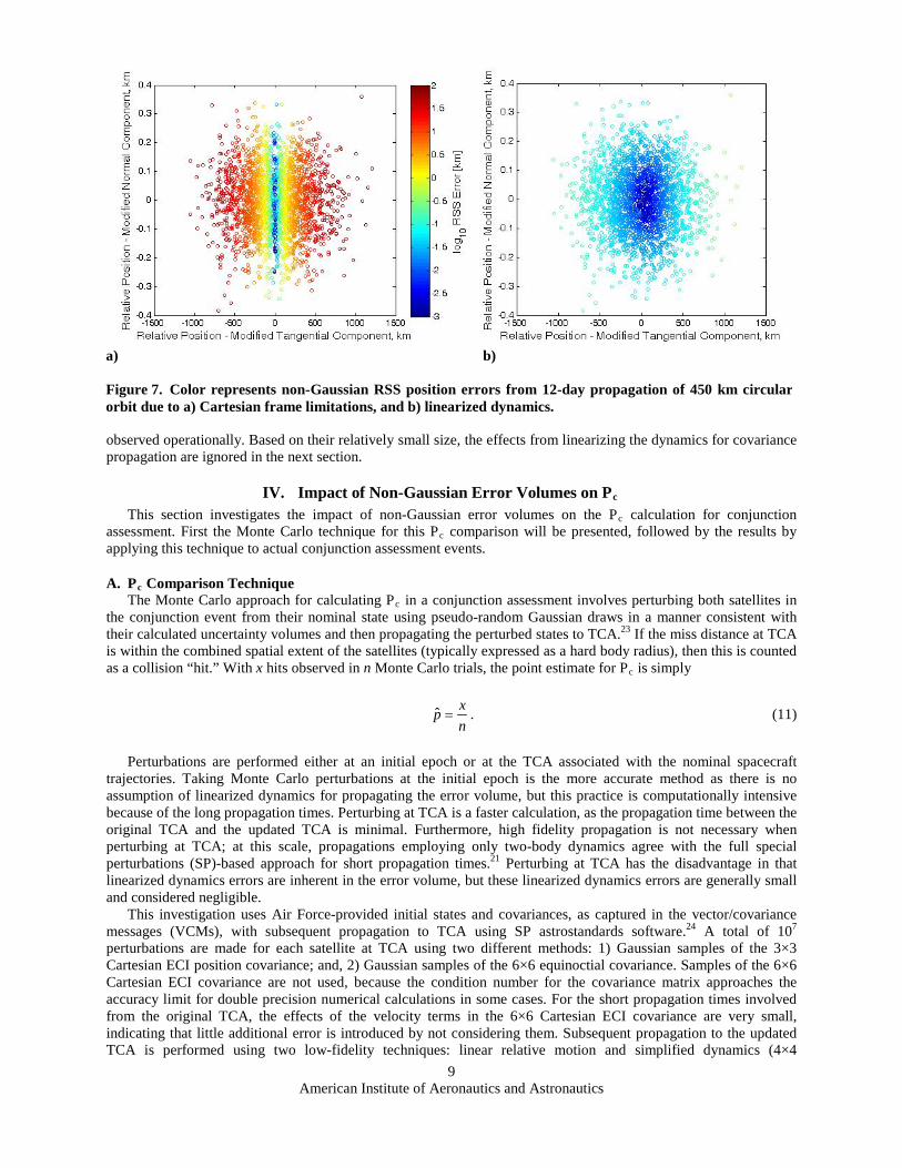
Two examples are considered. Both are synthetic examples with larger-than-typical covariance values in an attempt to try to highlight the linearization errors. The first case is a 450 km by 6200 km orbit with initial ECI position covariance diagonal elements of 0.2 km, 0.2 km, 0.32 km respectively, and a propagation time of two days. The non-Gaussian root-sum-square (RSS) position error associated with Cartesian coordinates and linearized dynamics appears in Fig. 6. The total non-Gaussian deviation is the sum of these two terms. The color bar represents the position error on a logarithmic scale. Each point represents the comparison of a single Monte Carlo perturbation as compared with the nominal state. The NT-coordinates have been modified in two ways to make the figure clearer. First, the nominal NT-coordinates are rotated by the position uncertainty misalignment angle so that the Cartesian coordinates error is aligned with the rotated T-axis. Second, as the non-Gaussian error magnitude is already represented by the color scale, the deviation from a Gaussian distribution is removed from each point in the displayed NT-coordinates. Thus the distribution of points is consistent with a Gaussian. For this example, essentially all of the linearized dynamics errors are in the tangential direction, which makes it more difficult to observe as the position covariance is largest in this direction. The second case, appearing in Fig. 7, is based on a 450 km circular orbit with initial ECI position covariance diagonal elements of 0.1 km, 0.1 km, 0.2 km respectively, and a propagation time of 12 days. Here the linearized dynamics errors have non-zero components in both the tangential and normal directions. It is interesting to note that Fujimoto et al.11

In the examples depicted in Fig. 6 and Fig. 7, the linearized dynamics errors are small compared with the Cartesian frame limitations. Any numerical errors, such as those arising from the state error transition matrix and the Jacobian transformation, are included in this linearized dynamics error term. It is improbable that the numerical error vector would negate the linearized dynamics error vector for every point evaluated, so the general behavior is indicative of the linearized dynamics errors. Using a realistic (i.e., small) initial covariance results in negligible linearized dynamics errors. This study uses an osculating ECI propagation of the covariance whereas, operationally, the NASA Robotic CARA task exploits the results from Air Force Astrodynamics Support Workstation (ASW) propagation, which itself employs an osculating equinoctial propagation of the covariance. Equinoctial propagation of covariance has been shown to result in smaller linearized dynamics errors than Cartesian propagation of covariance.

observe that the linearized dynamics errors result in a bias in longitude, with the largest contribution to the bias coming from the ends of the error volume distribution. For a smaller-sized covariance, such as in Fig. 6, this bias in longitude would principally be observed in the tangential component, whereas in a larger covariance that covers a significant portion of the orbit, this bias in longitude would have both normal and tangential components.

7,10 Therefore, these results should be considered to be an upper bound on the linearized dynamics errors

a) b)

Figure 6. Color represents non-Gaussian RSS position errors from 2-day propagation of 450 km by 6200 km orbit due to a) Cartesian frame limitations, and b) linearized dynamics.

American Institute of Aeronautics and Astronautics

9

observed operationally. Based on their relatively small size, the effects from linearizing the dynamics for covariance propagation are ignored in the next section.

IV. Impact of Non-Gaussian Error Volumes on Pc

This section investigates the impact of non-Gaussian error volumes on the P c calculation for conjunction

assessment. First the Monte Carlo technique for this Pc

A. P

comparison will be presented, followed by the results by applying this technique to actual conjunction assessment events.

cThe Monte Carlo approach for calculating P

Comparison Technique c in a conjunction assessment involves perturbing both satellites in

the conjunction event from their nominal state using pseudo-random Gaussian draws in a manner consistent with their calculated uncertainty volumes and then propagating the perturbed states to TCA.23 If the miss distance at TCA is within the combined spatial extent of the satellites (typically expressed as a hard body radius), then this is counted as a collision “hit.” With x hits observed in n Monte Carlo trials, the point estimate for Pc

is simply

nxp =ˆ . (11)

Perturbations are performed either at an initial epoch or at the TCA associated with the nominal spacecraft trajectories. Taking Monte Carlo perturbations at the initial epoch is the more accurate method as there is no assumption of linearized dynamics for propagating the error volume, but this practice is computationally intensive because of the long propagation times. Perturbing at TCA is a faster calculation, as the propagation time between the original TCA and the updated TCA is minimal. Furthermore, high fidelity propagation is not necessary when perturbing at TCA; at this scale, propagations employing only two-body dynamics agree with the full special perturbations (SP)-based approach for short propagation times.21

This investigation uses Air Force-provided initial states and covariances, as captured in the vector/covariance messages (VCMs), with subsequent propagation to TCA using SP astrostandards software.

Perturbing at TCA has the disadvantage in that linearized dynamics errors are inherent in the error volume, but these linearized dynamics errors are generally small and considered negligible.

24 A total of 107 perturbations are made for each satellite at TCA using two different methods: 1) Gaussian samples of the 3×3 Cartesian ECI position covariance; and, 2) Gaussian samples of the 6×6 equinoctial covariance. Samples of the 6×6 Cartesian ECI covariance are not used, because the condition number for the covariance matrix approaches the accuracy limit for double precision numerical calculations in some cases. For the short propagation times involved from the original TCA, the effects of the velocity terms in the 6×6 Cartesian ECI covariance are very small, indicating that little additional error is introduced by not considering them. Subsequent propagation to the updated TCA is performed using two low-fidelity techniques: linear relative motion and simplified dynamics (4×4

a) b)

Figure 7. Color represents non-Gaussian RSS position errors from 12-day propagation of 450 km circular orbit due to a) Cartesian frame limitations, and b) linearized dynamics.

American Institute of Aeronautics and Astronautics

10

geopotential with drag and solar radiation pressure disabled). A combined hard body radius of 20 m is employed for determining whether or not the Monte Carlo perturbations result in a hit.

The input data set for this study comprise 248 historical, high risk (Pc ≥ 10–4

B. P

) conjunction events in various LEO orbits from the NASA Robotic CARA task database, ranging from 2006 to the present. Orbital properties for the primary (asset) and secondary objects as well as the corresponding distribution of propagation times appear in Fig. 8. Propagation times for the primary objects encompass the typical operational timeline for these conjunction assessments, or up to seven days. The secondary objects have a wider distribution of propagation times, because many of these objects are not as well-tracked as the primary objects.

cFor each conjunction event, the two Monte Carlo P

Comparison Results c

point estimates are calculated using Eq. (11) from sampling the 3×3 Cartesian ECI position covariance (“Cart”) and the 6x6 equinoctial covariance (“eq”) respectively, that is,

nx

pn

xp eqeq

CartCart == ˆ;ˆ . (12)

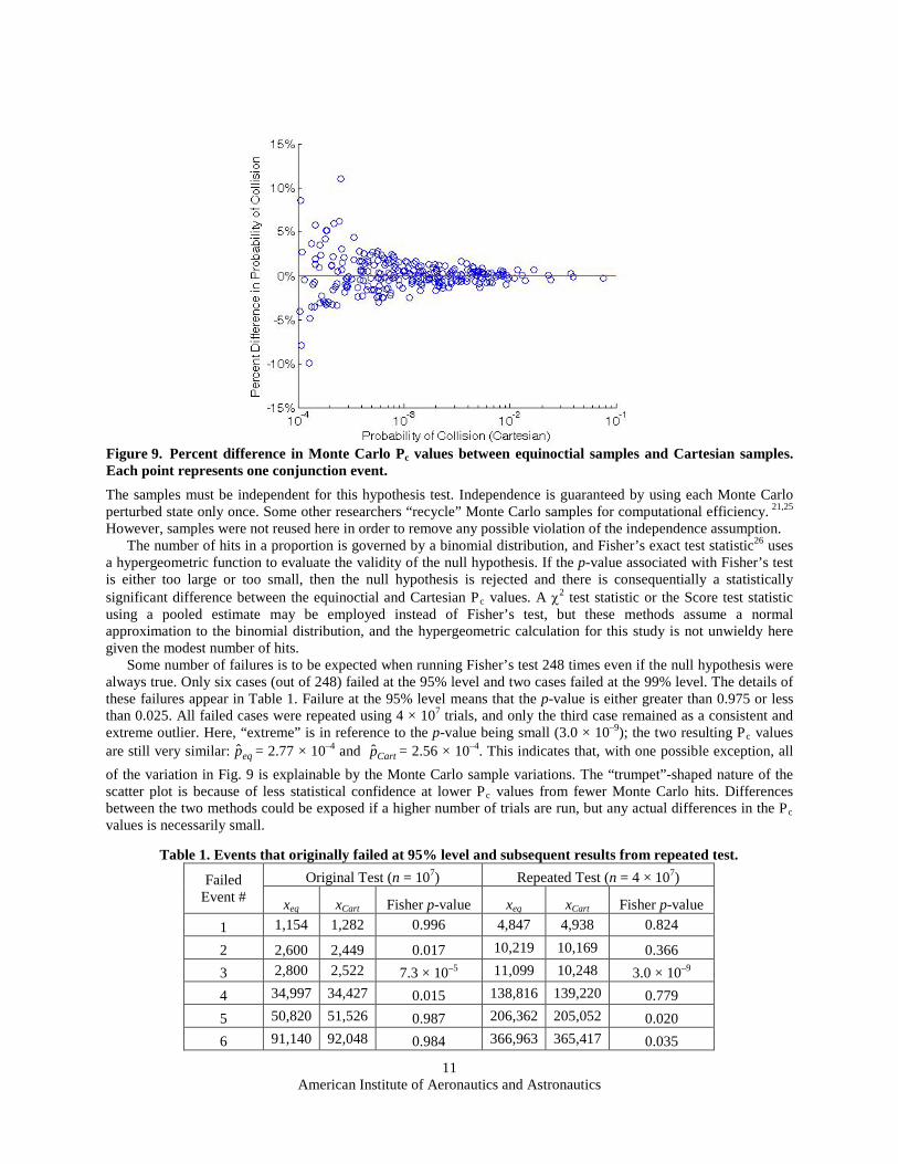
The combined results from the Pc ( ) CartCarteq ppp ˆˆˆ − comparison are displayed in Fig. 9, which displays , the percent difference between the two Monte Carlo calculations. Each point in the plot corresponding to a single event. The agreement between the two Monte Carlo methods is within ±15% for all cases. From the perspective of the CARA task, an order of magnitude or more change in Pc

Because Monte Carlo methods are based on random sampling, it is natural to question how much of the variability in Fig. 9 may be explained by the Monte Carlo samples. To answer this question, a statistical test is employed to compare two proportions; this test is separately performed for each conjunction event to compare the pair of point estimates calculated using Eq. (12). The null hypothesis for each statistical test is that the two P

would be considered significant, so none of the differences observed here are of operational significance.

c

values are equivalent:

Carteq ppH =:0 . (13)

a) b)

Figure 6. Non-Gaussian RSS position errors from 2 day propagation of 450x6200 km orbit due to (a) linearized coordinates, and (b) linearized dynamics.

a) b)

Figure 7. Non-Gaussian RSS position errors from 12 day propagation of 450 km circular orbit due to (a) linearized coordinates, and (b) linearized dynamics.

a) b)

Figure 8. Characteristics of primary and secondary objects used in Pc comparison study. a) Distribution of perigee and apogee heights, and b) distribution of propagation times.

American Institute of Aeronautics and Astronautics

11

The samples must be independent for this hypothesis test. Independence is guaranteed by using each Monte Carlo perturbed state only once. Some other researchers “recycle” Monte Carlo samples for computational efficiency. 21,25

The number of hits in a proportion is governed by a binomial distribution, and Fisher’s exact test statisticHowever, samples were not reused here in order to remove any possible violation of the independence assumption.

26 uses a hypergeometric function to evaluate the validity of the null hypothesis. If the p-value associated with Fisher’s test is either too large or too small, then the null hypothesis is rejected and there is consequentially a statistically significant difference between the equinoctial and Cartesian Pc values. A χ2

Some number of failures is to be expected when running Fisher’s test 248 times even if the null hypothesis were always true. Only six cases (out of 248) failed at the 95% level and two cases failed at the 99% level. The details of these failures appear in Table 1. Failure at the 95% level means that the p-value is either greater than 0.975 or less than 0.025. All failed cases were repeated using 4 × 10

test statistic or the Score test statistic using a pooled estimate may be employed instead of Fisher’s test, but these methods assume a normal approximation to the binomial distribution, and the hypergeometric calculation for this study is not unwieldy here given the modest number of hits.

7 trials, and only the third case remained as a consistent and extreme outlier. Here, “extreme” is in reference to the p-value being small (3.0 × 10–9); the two resulting Pc

eqp values

are still very similar: = 2.77 × 10–4Cartp and = 2.56 × 10–4. This indicates that, with one possible exception, all

of the variation in Fig. 9 is explainable by the Monte Carlo sample variations. The “trumpet”-shaped nature of the scatter plot is because of less statistical confidence at lower Pc values from fewer Monte Carlo hits. Differences between the two methods could be exposed if a higher number of trials are run, but any actual differences in the Pc values is necessarily small.

Figure 9. Percent difference in Monte Carlo Pc values between equinoctial samples and Cartesian samples. Each point represents one conjunction event.

Table 1. Events that originally failed at 95% level and subsequent results from repeated test.

Failed Event #

Original Test (n = 107) Repeated Test (n = 4 × 107)

xeq xCart Fisher p-value xeq xCart Fisher p-value 1 1,154 1,282 0.996 4,847 4,938 0.824

2 2,600 2,449 0.017 10,219 10,169 0.366 3 2,800 2,522 7.3 × 10–5 11,099 10,248 3.0 × 10–9 4 34,997 34,427 0.015 138,816 139,220 0.779 5 50,820 51,526 0.987 206,362 205,052 0.020 6 91,140 92,048 0.984 366,963 365,417 0.035

American Institute of Aeronautics and Astronautics

12

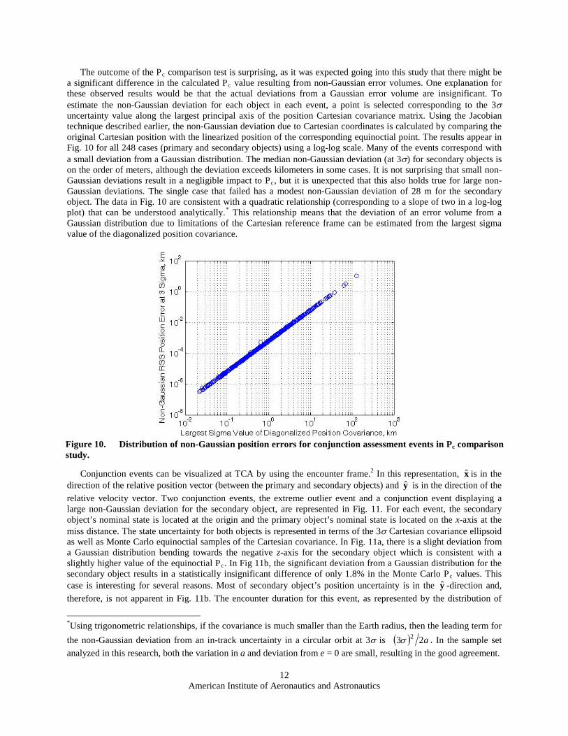
The outcome of the Pc comparison test is surprising, as it was expected going into this study that there might be a significant difference in the calculated Pc value resulting from non-Gaussian error volumes. One explanation for these observed results would be that the actual deviations from a Gaussian error volume are insignificant. To estimate the non-Gaussian deviation for each object in each event, a point is selected corresponding to the 3σ uncertainty value along the largest principal axis of the position Cartesian covariance matrix. Using the Jacobian technique described earlier, the non-Gaussian deviation due to Cartesian coordinates is calculated by comparing the original Cartesian position with the linearized position of the corresponding equinoctial point. The results appear in Fig. 10 for all 248 cases (primary and secondary objects) using a log-log scale. Many of the events correspond with a small deviation from a Gaussian distribution. The median non-Gaussian deviation (at 3σ) for secondary objects is on the order of meters, although the deviation exceeds kilometers in some cases. It is not surprising that small non-Gaussian deviations result in a negligible impact to Pc, but it is unexpected that this also holds true for large non-Gaussian deviations. The single case that failed has a modest non-Gaussian deviation of 28 m for the secondary object. The data in Fig. 10 are consistent with a quadratic relationship (corresponding to a slope of two in a log-log plot) that can be understood analytically.*

Conjunction events can be visualized at TCA by using the encounter frame.

This relationship means that the deviation of an error volume from a Gaussian distribution due to limitations of the Cartesian reference frame can be estimated from the largest sigma value of the diagonalized position covariance.

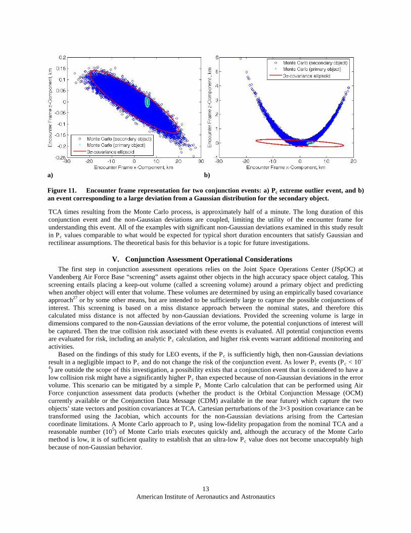
2 x In this representation, is in the direction of the relative position vector (between the primary and secondary objects) and y is in the direction of the relative velocity vector. Two conjunction events, the extreme outlier event and a conjunction event displaying a large non-Gaussian deviation for the secondary object, are represented in Fig. 11. For each event, the secondary object’s nominal state is located at the origin and the primary object’s nominal state is located on the x-axis at the miss distance. The state uncertainty for both objects is represented in terms of the 3σ Cartesian covariance ellipsoid as well as Monte Carlo equinoctial samples of the Cartesian covariance. In Fig. 11a, there is a slight deviation from a Gaussian distribution bending towards the negative z-axis for the secondary object which is consistent with a slightly higher value of the equinoctial Pc. In Fig 11b, the significant deviation from a Gaussian distribution for the secondary object results in a statistically insignificant difference of only 1.8% in the Monte Carlo Pc

y values. This

case is interesting for several reasons. Most of secondary object’s position uncertainty is in the -direction and, therefore, is not apparent in Fig. 11b. The encounter duration for this event, as represented by the distribution of

*Using trigonometric relationships, if the covariance is much smaller than the Earth radius, then the leading term for the non-Gaussian deviation from an in-track uncertainty in a circular orbit at 3σ is ( ) a23 2σ . In the sample set analyzed in this research, both the variation in a and deviation from e = 0 are small, resulting in the good agreement.

Figure 10. Distribution of non-Gaussian position errors for conjunction assessment events in Pc comparison study.

American Institute of Aeronautics and Astronautics

13

TCA times resulting from the Monte Carlo process, is approximately half of a minute. The long duration of this conjunction event and the non-Gaussian deviations are coupled, limiting the utility of the encounter frame for understanding this event. All of the examples with significant non-Gaussian deviations examined in this study result in Pc

V. Conjunction Assessment Operational Considerations

values comparable to what would be expected for typical short duration encounters that satisfy Gaussian and rectilinear assumptions. The theoretical basis for this behavior is a topic for future investigations.

The first step in conjunction assessment operations relies on the Joint Space Operations Center (JSpOC) at Vandenberg Air Force Base “screening” assets against other objects in the high accuracy space object catalog. This screening entails placing a keep-out volume (called a screening volume) around a primary object and predicting when another object will enter that volume. These volumes are determined by using an empirically based covariance approach27 or by some other means, but are intended to be sufficiently large to capture the possible conjunctions of interest. This screening is based on a miss distance approach between the nominal states, and therefore this calculated miss distance is not affected by non-Gaussian deviations. Provided the screening volume is large in dimensions compared to the non-Gaussian deviations of the error volume, the potential conjunctions of interest will be captured. Then the true collision risk associated with these events is evaluated. All potential conjunction events are evaluated for risk, including an analytic Pc

Based on the findings of this study for LEO events, if the P

calculation, and higher risk events warrant additional monitoring and activities.

c is sufficiently high, then non-Gaussian deviations result in a negligible impact to Pc and do not change the risk of the conjunction event. As lower Pc events (Pc < 10–

4) are outside the scope of this investigation, a possibility exists that a conjunction event that is considered to have a low collision risk might have a significantly higher Pc than expected because of non-Gaussian deviations in the error volume. This scenario can be mitigated by a simple Pc Monte Carlo calculation that can be performed using Air Force conjunction assessment data products (whether the product is the Orbital Conjunction Message (OCM) currently available or the Conjunction Data Message (CDM) available in the near future) which capture the two objects’ state vectors and position covariances at TCA. Cartesian perturbations of the 3×3 position covariance can be transformed using the Jacobian, which accounts for the non-Gaussian deviations arising from the Cartesian coordinate limitations. A Monte Carlo approach to Pc using low-fidelity propagation from the nominal TCA and a reasonable number (105) of Monte Carlo trials executes quickly and, although the accuracy of the Monte Carlo method is low, it is of sufficient quality to establish that an ultra-low Pc value does not become unacceptably high because of non-Gaussian behavior.

a) b) Figure 11. Encounter frame representation for two conjunction events: a) Pc extreme outlier event, and b) an event corresponding to a large deviation from a Gaussian distribution for the secondary object.

American Institute of Aeronautics and Astronautics

14

VI. Conclusions An initially Gaussian error volume will become non-Gaussian over time due to the nonlinear dynamics inherent

in propagation. The combination of linearizing the dynamical system for propagating the error volume (linearized dynamics) and representing the error volume in a Cartesian frame artificially suppresses the true non-Gaussian nature of the error volume as expressed by the state error covariance matrix. The limitations from representing the error volume in Cartesian coordinates dominate over linearized dynamics errors for typical conjunction assessment objects. Neglecting the linearized dynamics errors simplifies the processing for conjunction assessment, as retention of existing theories and propagation methods is permitted. A sufficient method to account for the non-Gaussian behavior addresses the limitations of Cartesian coordinates in representing the error volume: convert Gaussian Monte Carlo samples from the Cartesian covariance at TCA using the linearized Jacobian into osculating equinoctial elements, and use these perturbed states as the basis for a Monte Carlo calculation of Pc. Furthermore, performing this technique on a set of 248 LEO conjunctions with Pc ≥ 10–4 results in an operationally insignificant impact to calculating Pc, even in cases where the non-Gaussian deviation is significant. Although this is not an exhaustive sample, the results suggest that the impact to Pc from non-Gaussian error volumes is insignificant for high Pc cases. As state uncertainties represented by the covariance are generally small, and if the covariances are small, the non-Gaussian deviations are consequently small. The impact of non-Gaussian error volumes on low Pc events is not examined in this study but is mitigable using data products currently provided by the JSpOC using the proposed Pc

Appendix

Monte Carlo framework.

Let the spacecraft state vector equations of motion be represented by

( )t,xfx = . (A1)

State deviations at an initial time t0

can be mapped to state deviations at another time t using a state error transition matrix Φ:

( ) ( ) ( )00, tttt xΦx δδ = . (A2)

The state transition matrix can be numerically integrated by considering the following equation:

( ) ( ) ( )00 ,, ttttt ΦAΦ = (A3)

subject to the initial condition

( ) IΦ =00 , tt , (A4)

where I is an identity matrix of order six and the Jacobian matrix ( )tA is defined by

( ) ( )

( )

∂∂

∂∂

∂∂

∂∂

∂∂

∂∂

∂∂

∂∂

∂∂

∂∂

∂∂

∂∂

=∂∂

=

)()(

)()(

)()(

)()(

)()(

)()(

)()(

)()(

)()(

)()(

)()(

)()(

,

tztz

txtz

tztz

tytz

txtz

tzty

tyty

txty

tztx

tztx

tytx

txtx

ttt

xxfA . (A5)

This notation for this Jacobian presumes osculating ECI propagation as is used in this paper. The covariance matrix at time t can be expressed as

American Institute of Aeronautics and Astronautics

15

( ) ( ) ( ) ttEt TxxP δδ= (A6)

where ⋅E is the expectation operator. Substituting Eq. (A2) into Eq. (A6) leads to the result that covariance propagation can be written as

( ) ( ) ( ) ( )000 ,, tttttt TΦPΦP = , (A7)

which is the same similarity transformation shown as presented in Eq. (1). The coordinate representation of the dynamics is an inherent aspect of the nonlinearity of the problem, so changing the reference frame of propagation in Eq. (A1), for example from osculating ECI to osculating equinoctial, will affect the resulting linearized dynamics errors.

Acknowledgments This paper was supported by the NASA Goddard Space Flight Center (GSFC), Greenbelt, MD, under the Flight

Dynamics Support Services (FDSS) contract (NNG10CP02C), Task Order 21. The authors wish to thank Mrs. Lauri Newman for underwriting this research, Air Force Space Command, Studies and Analysis Division (AFSPC/A9) for astrodynamics tools and support, and Dr. Matt Hejduk for technical review of this material.

References 1Newman, L. K., Frigm, R., and McKinley, D., “It’s Not a Big Sky After All: Justification for a Close Approach Prediction

and Risk Assessment Process,” Advances in the Astronautical Sciences, edited by A. V. Rao, T. A. Lovell, F. K. Chan, and L. A. Cangahuala, Vol. 135, AAS, San Diego, 2009, pp. 1113-1132.

2Chan, F. K., “Spacecraft Collision Probability,” The Aerospace Press, El Segundo, CA, 2008, Chaps. 2, 3. 3National Research Council, “Limiting Future Collision Risk to Spacecraft: an Assessment of NASA’s Meteoroid and Orbital

Debris Programs,” National Academies Press, Washington, D.C., 2011, p.68. 4Sabol, C., Sukut, T., Hill, K., Alfriend, K. T., Wright, B., and Schumacher, P., “Linearized Orbit Covariance Generation and

Propagation Analysis via Simple Monte Carlo Simulations”, AFRL-RD-PS, TP-2010-1009. 5Junkins, J. L., and Singla, P., "How Nonlinear Is It? - A Tutorial on Nonlinearity of Orbit and Attitude Dynamics," Journal

of Astronautical Sciences, Vol 52, No. 1-2, 7-60, 2004. 6Horwood, J. T., Aragon, N. D., and Poore, A. B., “Edgeworth Filters for Space Surveillance Tracking,” 2010 Advanced

Maui Optical and Space Surveillance Technologies Conference Proceedings, Maui Economic Development Board, Maui, pp. 268-277.

7Junkins, J. L., Akella, M. R., and Alfriend, K. T., “Non-Gaussian Error Propagation in Orbit Mechanics,” Journal of the Astronautical Sciences, Vol. 44, No. 4, 1996, pp. 541–563.

8Hoots, F. R., “Satellite Location Uncertainty Prediction,” Advances in the Astronautical Sciences, edited by H. Schaub, B. C. Gunter, R. P. Russell, and W. T. Cerven, Vol. 142, AAS, San Diego, 2011, pp. 2759-2768.

9Folcik, Z., Lue, A., and Vatsky, J., “Reconciling Covariances with Reliable Orbital Uncertainty,” 2011 Advanced Maui Optical and Space Surveillance Technologies Conference Proceedings, Maui Economic Development Board, Maui, pp. 309-318.

10Horwood, J. T., Aragon, N. D., and Poore, A. B., “Gaussian Sum Filters for Space Surveillance: Theory and Simulations,” AIAA Journal for Guidance, Control and Dynamics, 34(6), Nov.-Dec. 2011, pp. 1839-1851.

11Fuijimoto, K., Scheeres, D. J., and Alfriend, K. T., “Analytic Non-linear Propagation of Uncertainty in the Two-Body Problem,” Journal of Guidance, Control, and Dynamics, Vol. 35, No. 2, March-April 2012, pp. 497-509.

12Jones, B. A., Doostan, A., and Born, G. H., “Nonlinear Propagation of Orbit Uncertainty Using Non-Intrusive Polynomial Chaos,” AIAA Journal for Guidance, Control and Dynamics (to be published).

13Hill, K., Alfriend, K. T., and Sabol, C., “Covariance-based Uncorrelated Track Association,” AIAA 2008-7211, AIAA/AAS Astrodynamics Specialist Conference, Honolulu, HI, August 18-21, 2008.

14Vallado, D. A., and Alfano, S., “Curvilinear Coordinates for Covariance and Relative Motion Operators,” Advances in the Astronautical Sciences, edited by H. Schaub, B. C. Gunter, R. P. Russell, and W. T. Cerven, Vol. 142, AAS, San Diego, 2011, pp. 929-946.

15Park, R. S., and Scheeres, D. J., “Nonlinear Mapping of Gaussian Statistics: Theory and Application to Spacecraft Design”, AIAA Journal for Guidance, Control and Dynamics, Vol. 29, No. 6, Nov.-Dec. 2006, pp. 1367-1375.

16Majji, M., Junkins, J. L., and Turner, J. D., “A High Order Method for Estimation of Dynamical Systems,” Journal of the Astronautical Sciences, Vol. 56, No. 3, 2008, pp. 401-440.

17Alspach, D. and Sorenson, H., “Nonlinear Bayesian Estimation Using Gaussian Sum Approximations," IEEE Transactions on Automatic Control, Vol. 17, No. 4, pp. 439-448, 1972.

18Giza, D., Singla, P., and Jah, M., “An Approach for Nonlinear Uncertainty Propagation: Application to Orbital Mechanics,” AIAA-2009-6082, AIAA Guidance, Navigation, and Control Conference, Chicago, Illinois, August 10-13, 2009.

American Institute of Aeronautics and Astronautics

16

19DeMars, K. J., Bishop, R. H., and Jah, M. K., “A Splitting Gaussian Mixture Method for the Propagation of Uncertainty in Orbital Mechanics,” AAS 11-201, Advances in the Astronautical Sciences, edited by M. K. Jah, Y. Guo, A. L. Bowes, and P. C. Lai, Vol. 140, AAS, San Diego, 2011.

20Tanygin, S., and Coppola, V. T., “Survey of Orbit Non-Linearity Effects in the Space Catalog,” AAS 10-202, Advances in the Astronautical Sciences, edited by D. Mortari, T. F. Starchville, Jr., A. J. Trask, and J. K. Miller, Vol. 136, AAS, San Diego, 2010.

21Sabol, C., Binz, C., Segerman, A., Roe, K., and Schumacher, Jr., P.W., “Probability of Collision with Special Perturbations Dynamics Using the Monte Carlo Method,” Advances in the Astronautical Sciences, edited by H. Schaub, B. Gunter, R. Russell, and W. Cerven, Vol. 142, AAS, San Diego, 2011, pp. 1081-1094.

22Cefola, P. J., Sabol, C., Hill, K., and Nishimoto, D., “Demonstration of the DSST State Transition Matrix Time-Update Properties Using the Linux GTDS Program,” 2011 Advanced Maui Optical and Space Surveillance Technologies Conference Proceedings, Maui Economic Development Board, Maui, pp. 260-269.

23Alfano, S., “Satellite Conjunction Monte Carlo Analysis,” Advances in the Astronautical Sciences, edited by A. M. Segerman, P. C. Lai, M. P. Wilkins, and M. E. Pittelkau, Vol. 134, AAS, San Diego, 2009, pp. 2007-2024.

24SPADOC Computation Center, “Mathematical Foundation for SCC Astrodynamic Theory,” NORAD Technical Publication TP-SCC-008, Headquarters North American Aerospace Defense Command, April 6 1982.

25de Vries, W. H., and Phillion, D. W., “Monte Carlo Method for Collision Probability Calculations Using 3D Satellite Models,” 2010 Advanced Maui Optical and Space Surveillance Technologies Conference Proceedings, Maui Economic Development Board, Maui, pp. 123-132.

26Fisher, R. A., "On the Interpretation of χ2 from Contingency Tables, and the Calculation of P," Journal of the Royal Statistical Society, Vol. 85, No. 1, pp. 87–94, 1922.

27Narvet, S. W., Frigm, R. C., and Hejduk, M. D., “Assessment of Uncertainty-Based Screening Volumes for NASA Robotic LEO and GEO Conjunction Risk Assessment,” Advances in the Astronautical Sciences, edited by H. Schaub, B. C. Gunter, R. P. Russell, and W. T. Cerven, Vol. 142, AAS, San Diego, 2011, pp. 1035-1052.