ORIGINAL PAPER

Impact of mathematical pharmacology on practice and theory:four case studies

Lambertus A. Peletier1 • Johan Gabrielsson2

Received: 27 April 2017 / Accepted: 18 August 2017 / Published online: 7 September 2017

� The Author(s) 2017. This article is an open access publication

Abstract Drug-discovery has become a complex disci-

pline in which the amount of knowledge about human

biology, physiology, and biochemistry have increased. In

order to harness this complex body of knowledge mathe-

matics can play a critical role, and has actually already

been doing so. We demonstrate through four case studies,

taken from previously published data and analyses, what

we can gain from mathematical/analytical techniques when

nonlinear concentration-time courses have to be trans-

formed into their equilibrium concentration-response (tar-

get or complex) relationships and new structures of drug

potency have to be deciphered; when pattern recognition

needs to be carried out for an unconventional response-

time dataset; when what-if? predictions beyond the obser-

vational concentration-time range need to be made; or

when the behaviour of a semi-mechanistic model needs to

be elucidated or challenged. These four examples are

typical situations when standard approaches known to the

general community of pharmacokineticists prove to be

inadequate.

Keywords Receptors � Drug-disposition � Dose-response-

time analysis � Michaelis-menten � Quasi-steady-state �Singular perturbations

Introduction

In recent years application of mathematics in drug devel-

opment has gained momentum. Even the FDA is consid-

ering approval of compounds in part on the basis of

arguments based on modelling and simulation (cf. [1]). But

there is a great variety of ways in which mathematics can

play a role in drug discovery and development. On the one

hand, the industrial scientist is often faced with the prob-

lem to make reliable predictions about such issues as

optimal dose or assessment of safety, on the basis of data

about onset, intensity and duration of response, when

quantitative information about the underlying mechanism

of action is limited. The challenge is then to combine

available physiological knowledge, well-designed experi-

ments and mathematical analysis to develop a model which

can be used to make such reliable predictions. In addition,

with expanding knowledge about biological and physio-

logical processes, more systems-based studies are being

carried out in which mathematical ideas about dynamical

systems are used, for instance, to model complex regula-

tory networks, or gain insight in the behaviour of such

networks, i.e. locate sensitive spots (cf. [2, 3]).

We demonstrate the role mathematics can play in vari-

ous aspects of pharmacology, such as (i) analysing com-

plex data sets; (ii) using mathematical reasoning for

dissecting model structure and acquiring quantitive infor-

mation out of unconventional response-time courses; (iii)

predicting the effect of chronic drug exposure on the basis

of relatively short-time data sets in the context of disease

& Lambertus A. Peletier

peletier@math.leidenuniv.nl

Johan Gabrielsson

johan.gabrielsson@slu.se

1 Mathematical Institute, Leiden University, PB 9512,

2300 RA Leiden, The Netherlands

2 Division of Pharmacology and Toxicology, Department of

Biomedical Sciences and Veterinary Public Health, Swedish

University of Agricultural Sciences, Box 7028,

750 07 Uppsala, Sweden

123

J Pharmacokinet Pharmacodyn (2018) 45:3–21

https://doi.org/10.1007/s10928-017-9539-8

progression. Finally, (iv) we show how mathematical

analysis can help to discover when a model is not Well-

Posed1 [4]. and statistical analysis yields unexpected and

counter-intuitive results. We discuss these examples of

mathematics in four case studies:

1. Probing the complexity of Target-Mediated Drug

Disposition.

2. Using Visual Inspection to estimate model parame-

ters—pattern recognition.

3. Model predictions beyond the experimental range.

4. Vetting a model that yields counter-intuitive concen-

tration-versus-time graphs.

The analyses presented in these four cases are based on

results published in, respectively [5–8].

Probing the complexity of target-mediated drugdisposition

Large molecule compounds, such as monoclonal antibod-

ies, exhibit interesting nontrivial interactions with their

target, involving binding, saturation and target turnover.

This results in complex ligand-concentration versus time

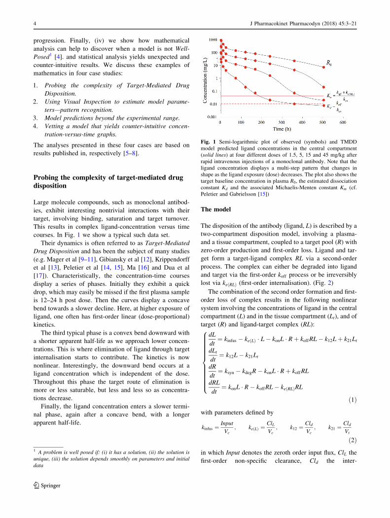
courses. In Fig. 1 we show a typical such data set.

Their dynamics is often referred to as Target-Mediated

Drug Disposition and has been the subject of many studies

(e.g. Mager et al [9–11], Gibiansky et al [12], Krippendorff

et al [13], Peletier et al [14, 15], Ma [16] and Dua et al

[17]). Characteristically, the concentration-time courses

display a series of phases. Initially they exhibit a quick

drop, which may easily be missed if the first plasma sample

is 12–24 h post dose. Then the curves display a concave

bend towards a slower decline. Here, at higher exposure of

ligand, one often has first-order linear (dose-proportional)

kinetics.

The third typical phase is a convex bend downward with

a shorter apparent half-life as we approach lower concen-

trations. This is where elimination of ligand through target

internalisation starts to contribute. The kinetics is now

nonlinear. Interestingly, the downward bend occurs at a

ligand concentration which is independent of the dose.

Throughout this phase the target route of elimination is

more or less saturable, but less and less so as concentra-

tions decrease.

Finally, the ligand concentration enters a slower termi-

nal phase, again after a concave bend, with a longer

apparent half-life.

The model

The disposition of the antibody (ligand, L) is described by a

two-compartment disposition model, involving a plasma-

and a tissue compartment, coupled to a target pool (R) with

zero-order production and first-order loss. Ligand and tar-

get form a target-ligand complex RL via a second-order

process. The complex can either be degraded into ligand

and target via the first-order koff process or be irreversibly

lost via keðRLÞ (first-order internalisation). (Fig. 2)

The combination of the second order formation and first-

order loss of complex results in the following nonlinear

system involving the concentrations of ligand in the central

compartment (L) and in the tissue compartment (Lt), and of

target (R) and ligand-target complex (RL):

dL

dt¼ kinfus � keðLÞ � L� konL � Rþ koffRL� k12Lþ k21Lt

dLt

dt¼ k12L� k21Lt

dR

dt¼ ksyn � kdegR� konL � Rþ koffRL

dRL

dt¼ konL � R� koffRL� keðRLÞRL

8>>>>>>>>>><

>>>>>>>>>>:

ð1Þ

with parameters defined by

kinfus ¼Input

Vc

; keðLÞ ¼ClL

Vc

; k12 ¼ Cld

Vc

; k21 ¼ Cld

Vt

ð2Þ

in which Input denotes the zeroth order input flux, ClL the

first-order non-specific clearance, Cld the inter-

Fig. 1 Semi-logarithmic plot of observed (symbols) and TMDD

model predicted ligand concentrations in the central compartment

(solid lines) at four different doses of 1.5, 5, 15 and 45 mg/kg after

rapid intravenous injections of a monoclonal antibody. Note that the

ligand concentration displays a multi-step pattern that changes in

shape as the ligand exposure (dose) decreases. The plot also shows the

target baseline concentration in plasma R0, the estimated dissociation

constant Kd and the associated Michaelis-Menten constant Km (cf.

Peletier and Gabrielsson [15])

1 A problem is well posed if: (i) it has a solution, (ii) the solution is

unique, (iii) the solution depends smoothly on parameters and initial

data

4 J Pharmacokinet Pharmacodyn (2018) 45:3–21

123

compartmental distribution, and Vc and Vt the volume of

the central- and the tissue compartment.

Steady states

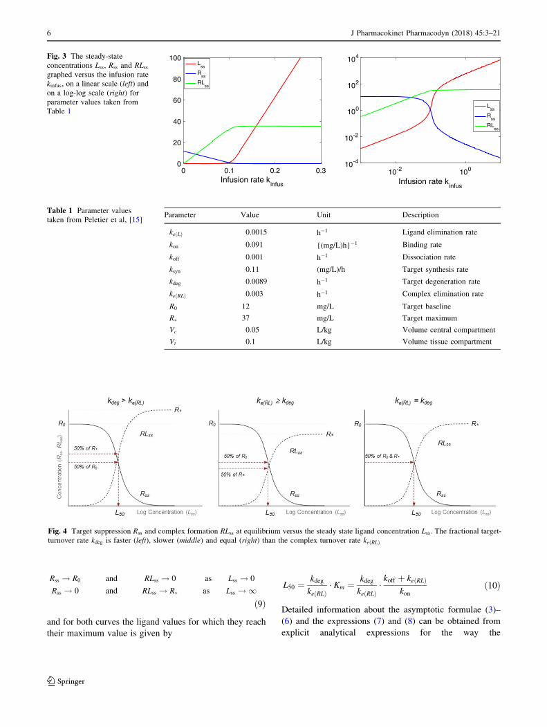
In Fig. 3 we show how the steady-state concentrations of

ligand, target and ligand-target complex vary as the infu-

sion rate kinfus changes when the parameter values are given

by Table 1. Note that at steady state the ligand concen-

trations in the central and the peripheral compartment are

the same.

For the values of Table 1, the dissociation constant is

Kd ¼ koff=kon ¼ 0:011 mg/L and the Michaelis-Menten

constant Km ¼ ðkoff þ keðRLÞÞ=kon ¼ 0:044 mg/L.

The graphs in Fig. 3 are complex and offer unique

diagnostic material to asses the strength of the different

processes and the values of the parameters under very

general conditions. Besides, whether or not there is a tissue

compartment makes no difference, the steady states are the

same.

The curves for Lss, Rss and RLss, have nontrivial shapes.

For instance, in the figure on the left in which they are

plotted linearly, they have the following properties:

(i) They each consist of two segments that are

approximately linear.

(ii) The two approximately linear segments are joined

at a narrow interface located at approximately

kinfus ¼ ksyn ¼ 0:11 (mg/L)/h.

Mathematical analysis

The slopes of these segments are well-defined and can be

computed explicitly. Hence, their dependence on the

parameters of the system (1) is transparent. Specifically, for

the ligand-receptor complex RL one can prove for the slope

(A) at low infusion rates:

RLss �A � kinfus as kinfus ! 0 where

A ¼def 1

keðRLÞ� R0

R0 þkeðLÞkeðRLÞ

Km

ð3Þ

At a critical value, when kinfus � ksyn, the growth of RL

stops abruptly and the graph becomes flat. The level (R�) at

which this happens is given by:

RLss ! R� ¼def ksyn

keðRLÞas kinfus ! 1 ð4Þ

Thus, the complex increases more or less linearly up to a

plateau where it abruptly levels off. The height of this

plateau depends on two parameters only: the synthesis rate

of receptor ksyn and the elimination rate keðRLÞ of ligand-

receptor complex.

Similarly, for the ligand Lss versus kinfus curve we find

for small infusion rates:

Lss �Km

R0

� A � kinfus as kinfus ! 0 ð5Þ

For the data of Table 1, Km � R0 so that the initial slope of

Lss is much smaller than that of RLss. This is also evident in

Fig. 3.

For large infusion rates it is possible to prove the fol-

lowing limit

Lss �1

keðLÞðkinfus � ksynÞ as kinfus ! 1 ð6Þ

This shows that Lss climbs as kinfus increases more or less

along a straight line with slope 1=keðLÞ and shifted to the

right by an amount equal to ksyn.

Because Lss depends monotonically on the infusion rate,

one can also express the steady state values of RL and R in

terms of the steady state ligand concentration. The result-

ing formula’s are

RLss ¼ R�Lss

Lss þ L50

and Rss ¼ R0

L50

Lss þ L50

ð7Þ

in which

R� ¼ksyn

keðRLÞ¼ kdeg

keðRLÞ� R0 and L50 ¼ kdeg

keðRLÞ� Km:

ð8Þ

According to (7) the graphs of Rss and RLss have a familiar

sigmoidal shape with different limits at large and small

ligand concentrations. They are shown in Fig. 4:

In particular, the limits at small and large ligand con-

centrations are given by

Fig. 2 Schematic description of target-mediated drug disposition.

Ligand L is distributed over a central- and a tissue compartment with

respective volumes Vc and Vt , is eliminated again via a first order

process (keðLÞ ¼ ClðLÞ=VcÞ, and binds reversibly (kon=koff ) to the target

R to form a ligand-target complex RL, which then is irreversibly

removed via a first order rate process (keðRLÞ)

J Pharmacokinet Pharmacodyn (2018) 45:3–21 5

123

Rss ! R0 and RLss ! 0 as Lss ! 0

Rss ! 0 and RLss ! R� as Lss ! 1ð9Þ

and for both curves the ligand values for which they reach

their maximum value is given by

L50 ¼ kdeg

keðRLÞ� Km ¼ kdeg

keðRLÞ�koff þ keðRLÞ

konð10Þ

Detailed information about the asymptotic formulae (3)–

(6) and the expressions (7) and (8) can be obtained from

explicit analytical expressions for the way the

0 0.1 0.2 0.3Infusion rate k

infus

0

20

40

60

80

100L

ss

Rss

RLss

10-2 100

Infusion rate kinfus

10-4

10-2

100

102

104

Lss

Rss

RLss

Fig. 3 The steady-state

concentrations Lss, Rss and RLss

graphed versus the infusion rate

kinfus, on a linear scale (left) and

on a log-log scale (right) for

parameter values taken from

Table 1

Table 1 Parameter values

taken from Peletier et al, [15]Parameter Value Unit Description

keðLÞ 0.0015 h�1 Ligand elimination rate

kon 0.091 {(mg/L)h}�1 Binding rate

koff 0.001 h�1 Dissociation rate

ksyn 0.11 (mg/L)/h Target synthesis rate

kdeg 0.0089 h�1 Target degeneration rate

keðRLÞ 0.003 h�1 Complex elimination rate

R0 12 mg/L Target baseline

R� 37 mg/L Target maximum

Vc 0.05 L/kg Volume central compartment

Vt 0.1 L/kg Volume tissue compartment

Fig. 4 Target suppression Rss and complex formation RLss at equilibrium versus the steady state ligand concentration Lss. The fractional target-

turnover rate kdeg is faster (left), slower (middle) and equal (right) than the complex turnover rate keðRLÞ

6 J Pharmacokinet Pharmacodyn (2018) 45:3–21

123

concentrations depend on the infusion rate kinfus. They are

given in Gabrielsson and Peletier [5].

Conclusion

We have seen how the complexity of the TMDD model is

elegantly depicted by plotting the steady states of the

compounds L, R and RL versus the infusion rate kinfus (cf.

Fig. 3). The graphs can be computed explicitly and depend

critically on the initial amount of target R0 and what one

could call a generalised dissociation constant which

combines dissociation and internalisation of ligand-target

complex:

Km ¼koff þ keðRLÞ

kon

ð11Þ

If Km � R0, a common situation (cf [10, 15, 18]), the

graphs are almost piece-wise linear and the explicit

expressions for the slopes are quite simple.

Dependence of target-ligand complex formation RL and

receptor suppression R on the ligand concentration, proves

to be described by graphs of simple sigmoidal functions

(cf. Fig. 4). This introduces a potency parameter L50 which

is related to Km by the quotient of the two target elimina-

tion rates kdeg and keðRLÞ:

L50 ¼ kdeg

keðRLÞ� Km ð12Þ

Thus, a close analysis of the steady state properties of the

three compounds involved in target-mediated disposition

reveals a great deal about the relative importance of the

sub-processes involved, and offers the possibility to

acquire quantitative information about them.

Using visual inspection to estimate modelparameters

This case study is aimed at demonstrating how mathe-

matical reasoning can be used to help the modeller in

choosing appropriate models on the basis of pharmacoki-

netic and pharmacodynamics data sets. This becomes

especially important when little is known about the

underlying pharmacokinetics, e.g., when the drug is not

supplied to the plasma. Thus, for such situations the only

data available are for response over time for different doses

and forms of administration. Study of such problems is

often referred to as dose-response-time analysis. It goes

back to early papers by Levy [19] and [20] and Smolen

[21]. For further references we refer to [6, 22–28]. Specific

questions such as (i) How does mathematical reasoning

address what is observed in onset, intensity and duration of

response, and (ii) How to choose an appropriate model are

discussed.

Data, model and equations

The data set records the locomotor activity, measured by

the number of times moving rats interrupted three light

beams in a cage when they were supplied by a drug,

(dexamphetamine). In the absence of dexamphetamine the

number of interruptions was negligible, but it goes up when

the drug is given. The exact mode of action of drug is not

known, and therefore an empirical mathematical model is

proposed.

Data shown in Fig. 5 were obtained and digitized from

Van Rossum and Van Koppen [29]. They recorded the

locomotor activity score after administration of dexam-

phetamine to rats at two dose levels (3.12 and 5.62 lg

kg-1). The data set was unusual because (i) the rise and

drop of response were approximately linear with time and

(ii) the slope of the increase and of the decline in the

locomotor activity score was independent of dose. In

addition, the transition from increase to decline was rela-

tively rapid.

Because the exposure to testcompound (drug) was not

known, a classic biophase model was fitted, one in which

the drug is administered through an intravenous bolus

administration. The amount of drug Ab in the biophase (in

lg) is described by the equation:

AbðtÞ ¼ F� � D � e�k t ð13Þ

where D denotes the dose (in lg), and F� the biophase

availability, i.e., the fraction of the dose that reaches the

biophase, and k the elimination rate of the drug out of the

biophase.

Fig. 5 Locomotor activity scores (number of interruptions per

minute)-versus-time data following two subcutaneous 3.12 and 5.62

lg kg-1 doses of dexamphetamine (Van Rossum and Van Koppen

[29]). The solid lines represent predictions from fitting the model (14)

to the experimental data. Note the apparently linear and parallel

decline in response over time independently of dose

J Pharmacokinet Pharmacodyn (2018) 45:3–21 7

123

The pharmacodynamic response R i.e., the number of

interruptions per minute, is assumed to be described by a

nonlinear turnover equation

dR

dt¼ FðAbÞ � kout;max �

R

Km þ Rð14Þ

in which FðAbÞ is the drug-mechanism function through

which the drug in the biophase impacts the response,

kout;max the maximal elimination rate and Km the response

at which the elimination rate is half-maximal. The com-

bined biophase- and pharmacodynamic model is depicted

in Fig. 6. Prior to administration of the compound no

activity is observed, i.e., Rð0Þ ¼ 0.

Two observations inform the selection of the function

FðAbÞ:

(i) The data exhibit a zero baseline. This means that

Fð0Þ ¼ 0.

(ii) As the drug dose increases, the initial slope of the

data curves appears to reach a maximum.

They suggest a saturable drug-mechanism function which

vanishes when the drug vanishes. It is of the following

form:

FðAbÞ ¼ Fmax

AnHb

FDnH50 þ AnH

b

ð15Þ

in which Fmax (response units �t�1), FD50 (dose units) and

nH correspond to the maximum drug-induced efficacy, the

potency and the Hill-exponent.

The particular form of the turnover eq. (14) was selected

in light of the approximately linear elimination of response

which suggest saturation.

Mathematical analysis

In order to proceed from qualitative observations to

quantitative estimates about the model, we employ the

following observations:

• Decline of the response: After the time Tmax of

maximal response the graph has three conspicuous

properties: (i) it is straight, (ii) it does not change with

drug dose, and (iii) it exhibits a sharp angle as it

approaches the baseline.

These characteristics of the response curve offer us an

unusual insight into the dynamics of the model.

(a) At the time of maximal response Tmax the drug has

been eliminated and FðAbÞ � 0, so that for t[ Tmax,

the turnover equation is approximately reduced to

dR

dt¼ �kout;max

R

Km þ Rð16Þ

When R � Km, then eq. (16) simplifies to

dR

dt¼ �kout;max ð17Þ

which shows that the slope of the graph is �kout;max.

On the basis of the data we obtain the estimate:

kout;max � 29 interruptions � minute�1 � h�1 ð18Þ

(b) The sharp angle of the graph of R(t) as it approaches

the baseline, i.e., when R � 0, can be accounted for

by a small value of Km.

(c) The response-time course associated with the higher

dose peaks at about Tmax ¼ 0:8 h. If one assumes that

approximately four half-lives have elapsed before

the drug has been cleared from the biophase, this

means that 4 t1=2 � 0:8 h, i.e., the half-life of the

drug in the biophase can be approximated by

t1=2 � 0:2 h; ð19Þ

and

k ¼ lnð2Þt1=2

� 3:5 h�1: ð20Þ

• Rise of the response For the higher dose the initial

segment of the graph of R(t) is approximately a straight

line. This suggest that during this period the stimulatory

function is saturated, so that FðAbÞ � Fmax, and,

Fig. 6 Schematic representation of the locomotor activity model

given by eqs. (13) and (14). Drug is supplied to the biophase,

eliminated through a first order process (k), and the amount of drug Ab

has a stimulating effect in the turnover equation for the response

through a nonlinear function FðAbÞ. Loss of response is modeled by a

saturable function with maximal (zeroth order) loss rate (kout;max), half

of which is reached when R ¼ Km

8 J Pharmacokinet Pharmacodyn (2018) 45:3–21

123

provided R � Km, the turnover equation is well

approximated by

dR

dt¼ Fmax � kout;max ð21Þ

Since the data show an initial slope (dR / dt) of 168

interruptions/minute/h, we deduce that Fmax � 168 þkout;max interruptions/minute/h. Using the estimate for

kout:max from the first observation, we conclude that

Fmax � 168 þ 29 ¼ 197 interruptions � minute�1 � h�1

ð22Þ

Remark It is evident from eq. (14) that at steady state, the

amount Ab;ss should be small enough so that the production

FðAb;ssÞ is smaller than the maximal rate of loss in order to

reach a steady state. Thus a basic assumption in this model

is that

FðAb;ssÞ\kout;max ð23Þ

• Time to maximal response Tmax. To obtain a ball park

value for the time to maximal response Tmax, we

approximate the function FðAbðtÞÞ, defined by (15), by

a step-function. This choice is based on the fact that, as

we argued before, the up-swing is more or less linear,

so that the function FðAbðtÞÞ appears saturated, and the

decline is also linear and in addition, dose-independent,

which suggests that FðAbðtÞÞ � 0 after the peak-time

Tmax. Thus, if AbðtÞ is decreasing and crosses the level

FD50, say at time T, i.e., when AbðTÞ ¼ FD50, then we

postulate that the function FðAbðtÞÞ can be approxi-

mated by the step function

FðAbðtÞÞ ¼ Fmax � HeavðT � tÞ ð24Þ

Here HeavðsÞ denotes the Heaviside function which

equals ?1 if s 0 and 0 if s\0. Thus, HeavðT � tÞ ¼ 1

if t� T and HeavðT � tÞ ¼ 0 if t[ T .

As the Hill-coefficient becomes larger, this approximation

improves, i.e.,

limnH!1

Fmax

AnHb

FDnH50 þ AnH

b

¼0 if Ab\FD50

Fmax if Ab [FD50

�

ð25Þ

This property follows readily from the classical limit

limn!1

xn

1 þ xn¼

0 if 0\x\1

1 if x[ 1

�

ð26Þ

The turnover eq. (14) can now be approximated by

dR

dt¼ Fmax � HeavðT � tÞ � kout;max as long as R[ 0

ð27Þ

except for when R is small, specifically, when R ¼ OðKmÞ.Starting at baseline, the solution R�ðtÞ of this equation is

given by:

R�ðtÞ ¼def ðFmax � kout;maxÞ t if 0� t� T

Fmax T � kout;max t if T\t\Tend

�

ð28Þ

where ð0; TendÞ is the maximal interval on which R�ðtÞ[ 0.

Since Fmax [ kout;max by eq. (23) it follows that R(t) is

increasing for 0\t\T . Plainly, R(t) is decreasing for

t[ T . Therefore Rmax ¼ RðTÞ, so that T ¼ TmaxðDÞ, and

TendðDÞ ¼Fmax

kout;max

� TmaxðDÞ ð29Þ

Because the biophase is assumed to follow intravenous

bolus dynamics, as described by eq. (13), it follows that

AbðTmaxÞ ¼ F� � D � e�k Tmax ¼ FD50 ð30Þ

We assumed that F� ¼ 1, had taken the larger dose D ¼5:62 lg kg-1, and estimated the elimination rate out of the

system to be k ¼ 3:5 h�1. By visual inspection, the time of

maximal response was estimated by Tmax ¼ 0:8. Thus, we

conclude from eq. (30) that the potency can be estimated as

follows:

FD50 ¼ 0:34 lg � kg�1: ð31Þ

Observe that for fixed Ab the steady-state response Rss is

formally given by

RssðAb;ssÞ ¼ Km � FðAb;ssÞkout;max � FðAb;ssÞ

ð32Þ

Recall that according to the assumption (23), we have

kout;max [FðAb;ssÞ.

Table 2 Model parameters for the locomotor activity example and

relative standard deviation (CV%)

Parameter Units Estimate Final est. CV%

k h�1 3.5 5.96 4

Fmax Resp h-1 197 249 4

FD50 lg kg-1 0.34 1.02 4

nH – – 1.63 5

kout;max Resp h-1 29 30.1 4

Km h�1 Small 0.001 9

J Pharmacokinet Pharmacodyn (2018) 45:3–21 9

123

Conclusion

Using mathematical methods we have been able to estimate

many of the parameters, such as k in the biophase model,

and Fmax and FD50, as well as kout;max and Km in the

pharmacodynamic model. These estimates can serve as

preliminary estimates for further refinement by statistical

software. By fitting the model (cf. equation (14)) to the

experimental response-time data in Fig. 5, the final

parameter estimates of Table 2 were obtained using the

nonlinear regression software WinNonlin 5.2 (Certara

Inc.).

The six model parameters generally had high precision

and were close to the analytically and graphically derived

initial parameter estimates. The mathematical reasoning in

the pattern recognition process thus proves to be useful

when unconventional data (as in this case) need to be

analysed.

Model predictions beyond the experimental range

Drug intake over long periods of time, such as is common

in the treatment of chronic diseases, may harbour risks

which are less evident over the period in which experi-

mental data is available. Simulations on the basis of

mathematical models, although predicated by the limited

availability of data, may then yield indications of what kind

of long time behaviour can be expected and how it can be

influenced.

Data, model and equations

We consider an example of such a situation discussed by

Peletier, de Winter and Vermeulen [7], in which data for

gIndiv idual predictionPopulation prediction1-receptor model

08406304202100840630420210

0 120 240 360 480

Time (hrs after 1st dose)

0

20

40

60

80

0

20

40

60

80

Plas

ma

conc

entra

tion

ID ID ID

ID ID ID

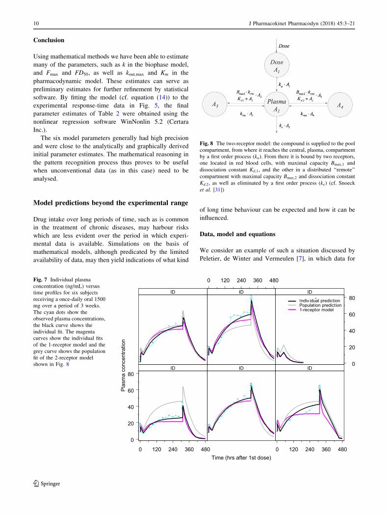
Fig. 7 Individual plasma

concentration (ng/mL) versus

time profiles for six subjects

receiving a once-daily oral 1500

mg over a period of 3 weeks.

The cyan dots show the

observed plasma concentrations,

the black curve shows the

individual fit. The magenta

curves show the individual fits

of the 1-receptor model and the

grey curve shows the population

fit of the 2-receptor model

shown in Fig. 8

Fig. 8 The two-receptor model: the compound is supplied to the pool

compartment, from where it reaches the central, plasma, compartment

by a first order process (ka). From there it is bound by two receptors,

one located in red blood cells, with maximal capacity Bmax;1 and

dissociation constant Kd;1, and the other in a distributed ‘‘remote’’

compartment with maximal capacity Bmax;2 and dissociation constant

Kd;2, as well as eliminated by a first order process (ke) (cf. Snoeck

et al. [31])

10 J Pharmacokinet Pharmacodyn (2018) 45:3–21

123

the plasma concentration of a compound was available for

a period of 480 hours. They are shown in Fig. 7.

This case-study involves a compound that is adminis-

tered into a pool compartment and absorbed in a central

compartment, from where it binds to two receptors through

Michaelis-Menten type reactions (cf. Michaelis and Men-

ten [30]) and dissociates according to first order kinetics.

The amounts (in mg) in pool- and central compartment are

denoted by, respectively, A1 and A2. Binding to one

receptor, which is probably located in the red blood cells is

fast (amount A3 mg) and binding to the other receptor,

which is located in what is called the ‘‘remote’’ compart-

ment, is slow (amount A4 mg). The distributional model is

illustrated in Fig. 8.

The model used to reach an optimal fit to the data shown

in Fig. 7 is based on a 2-receptor model due to Snoeck et al

[31] and is shown in Fig. 8. For comparison, the corre-

sponding 1-receptor model is obtained from the above

model by putting kRMT ¼ 0.

The 2-receptor model for the amounts of compound in

the four compartments (A1; . . .;A4) translates into the fol-

lowing set of differential equations:

dA1

dt¼ D � q� kaA1

dA2

dt¼ kaA1 � keA2 � Bmax;1kRBC

A2

Kd;1 þ A2

þ kRBCA3

� Bmax;2kRMT

A2

Kd;2 þ A2

þ kRMTA4

dA3

dt¼ Bmax;1kRBC

A2

Kd;1 þ A2

� kRBCA3

dA4

dt¼ Bmax;2kRMT

A2

Kd;2 þ A2

� kRMTA4

8>>>>>>>>>>>>>>>><

>>>>>>>>>>>>>>>>:

ð33Þ

where kRBC and kRMT are the distributional rate constants to

the receptors in the red blood cells and the remote recep-

tors, Bmax;1 and Bmax;2 the maximal capacity of these

receptors and Kd;1 and Kd;2 the associated dissociation

constants multiplied by the corresponding volumes. The

infusion rate is D � q mg/h, where q is the unit infusion rate,

i.e. q ¼ 1 mg/h and D is the amount of compound that is

supplied per hour.

It is assumed that initially, there is no compound in any

of the compartments or bound to the receptors, i.e.,

A1ð0Þ ¼ 0; A2ð0Þ ¼ 0; A3ð0Þ ¼ 0; A4ð0Þ ¼ 0:

ð34Þ

From t ¼ 0 onwards the compound is administered to the

pool compartment through a constant-rate infusion of D � qmg/h, which in this study is taken to be 40 mg/h.

Two models are used to fit the data, which are given in

aqua. The black curves are the individual fits made with the

2-receptor model (33) and the magenta curves are the

individual fits made with the 1-receptor model obtained

from the system (33) by putting kRMT ¼ 0. The grey curves

are the population fits made with the 2-receptor model. In

Table 3 we give the parameter values obtained by fitting

the 2-receptor model to the data.

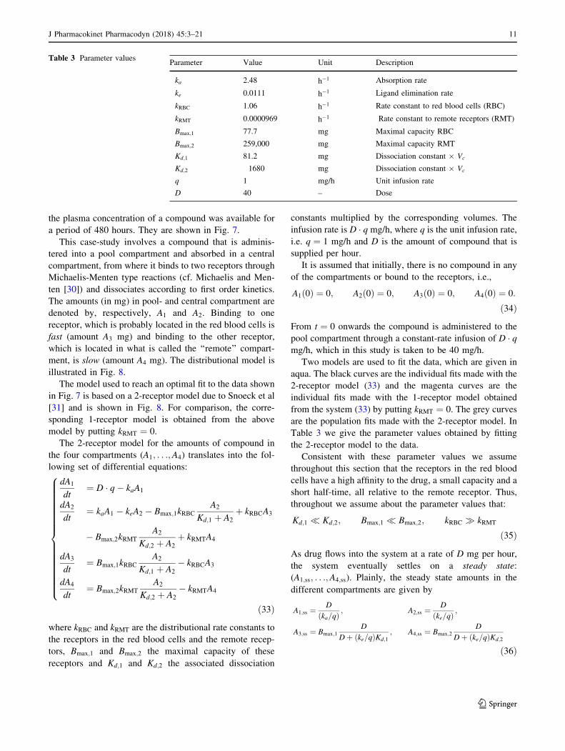
Consistent with these parameter values we assume

throughout this section that the receptors in the red blood

cells have a high affinity to the drug, a small capacity and a

short half-time, all relative to the remote receptor. Thus,

throughout we assume about the parameter values that:

Kd;1 � Kd;2; Bmax;1 � Bmax;2; kRBC � kRMT

ð35Þ

As drug flows into the system at a rate of D mg per hour,

the system eventually settles on a steady state:

(A1;ss; . . .;A4;ss). Plainly, the steady state amounts in the

different compartments are given by

A1;ss ¼D

ðka=qÞ; A2;ss ¼

D

ðke=qÞ;

A3;ss ¼ Bmax;1D

Dþ ðke=qÞKd;1; A4;ss ¼ Bmax;2

D

Dþ ðke=qÞKd;2

ð36Þ

Table 3 Parameter valuesParameter Value Unit Description

ka 2.48 h�1 Absorption rate

ke 0.0111 h�1 Ligand elimination rate

kRBC 1.06 h�1 Rate constant to red blood cells (RBC)

kRMT 0.0000969 h�1 Rate constant to remote receptors (RMT)

Bmax;1 77.7 mg Maximal capacity RBC

Bmax;2 259,000 mg Maximal capacity RMT

Kd;1 81.2 mg Dissociation constant Vc

Kd;2 1680 mg Dissociation constant Vc

q 1 mg/h Unit infusion rate

D 40 – Dose

J Pharmacokinet Pharmacodyn (2018) 45:3–21 11

123

Note that A1;ss and A2;ss are independent of the binding

constants and the capacities of the receptors, and increase

linearly with the infusion rate D.

Remark As a preliminary observation we note that the

first equation in the system (33) can be solved explicitly,

resulting in the following expression for A1ðtÞ:

A1ðtÞ ¼D � qka

ð1 � e�ka tÞ

Thus, A1ðtÞ ! A1;ss as t ! 1 with a half-life of t1=2 ¼lnð2Þ=ka ¼ 0:28 h, or 17 min. This is exceedingly short for

the time scale of interest. So effectively, it is permissible to

put A1ðtÞ � A1;ss. Therefore, we shall be mainly interested

in the amount of drug in the central or plasma compartment

and in the two types of receptors.

Simulations

In Fig. 9 we show how the amount of compound in the

plasma compartment, A2ðtÞ, evolves over time after the

infusion has been switched on. Evidently, two phases can

be distinguished: in the first phase, shown in the left panel,

A2 climbs to what appears to be a stationary state, which

we usually refer to as the Plateau value. Subsequently,

during a second phase, shown in the right panel, which

extends over a much longer time, A2 continues to climbs

towards its final steady state, albeit at a much slower pace.

In Fig. 10 we show simulations of the amount of com-

pound in the two receptors: A3 in the red blood cells and A4

in remote tissue. The left panel shows that A3 quickly

reaches a constant value, which is close to its final steady

state A3;ss (76.2 mg) computed from (36), the half-life

being about 5 h. The right panel shows how A4 evolves

over time and reaches its final steady state. Evidently, this

takes place on the same time scale as the second phase of

A2 shown in Fig. 9.

Summarising we distinguish three time scales in the

dynamics of the three-compartment model:

• The receptors in the red blood cells fill up fast.

Specifically, A3ðtÞ reaches its steady-state value with a

half-life of t1=2 ¼ Oð10Þ h,2 which is early compared to

the compound in the plasma compartment (A2) and in

the remote receptors (A4).

• The central compartment fills up in two phases: fairly

quickly up to an intermediate value, the Plateau Value

A2, with a half-life of t1=2 ¼ Oð102Þ h, and then much

more slowly, with a half-life of t1=2 ¼ Oð5 103Þ h, it

creeps up towards its final steady state A2;ss.

• The remote receptors fill up slowest: the amount of

drug A4ðtÞ reaches its steady-state level with a long

half-life t1=2 ¼ Oð104Þ h.

Mathematical analysis

In order to understand the observations made about the

simulations and answer such questions as (i) Which

receptor governs the dynamics in the initial phase? (ii)

How high does A2 rise in the first phase, i.e., what would be

a good estimate of the plateau value A2? (iii) What would

be the rate of convergence towards A2? and (iv) What is the

rate of convergence towards the final steady state in plasma

A2;ss, and analogous questions about the amount of drug in

the two types of receptors.

To answer these questions, we need to compare the

relative impact of the different terms in the system (33).

Because the amounts in the four compartments A1; . . .;A4

vary widely, as, do the rate constants given in Table 4, it is

necessary to transform to dimensionless variables and

normalise the amounts with well-chosen reference values.

0 200 400 600 800 1000Time (h)

0

1000

2000

3000

4000

5000

Am

ount

s (m

g)

A2

A3

A4

0 2 4 6 8 10Time (h) 104

0

1000

2000

3000

4000

5000

Am

ount

s (m

g)

A2

A3

A4

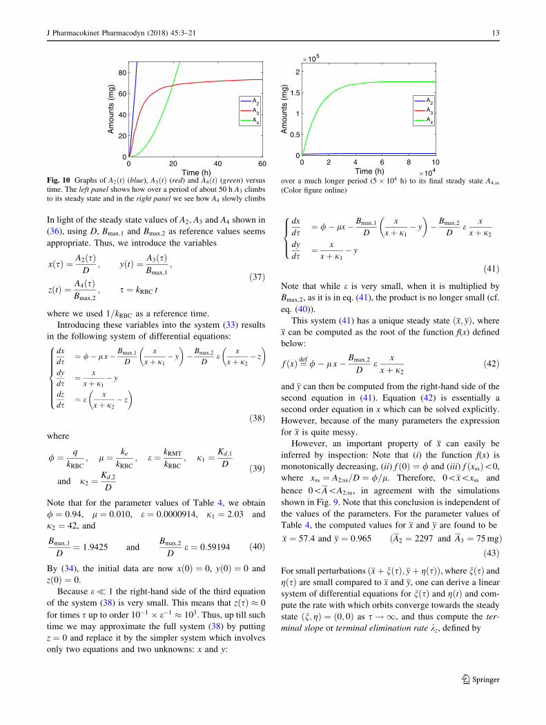
Fig. 9 Graphs show the amount versus time courses during a

constant-rate infusion over 103 and 105 h of compound in the second

compartment (A2ðtÞ (blue)), in the third (A3ðtÞ (red)) and the fourth

(A4ðtÞ (green)). The left panel shows how over a period of about 500

h A2 climbs to an intermediate steady state and the right panel shows

how A2 slowly climbs over a much longer period (5 104 h) to its

final steady state A2;ss. Details about the evolution of A3 and A4 are

shown in Fig. 10 (Color figure online)

2 T ¼ OðNÞ means that T is of the same order of magnitude as N.

12 J Pharmacokinet Pharmacodyn (2018) 45:3–21

123

In light of the steady state values of A2, A3 and A4 shown in

(36), using D, Bmax;1 and Bmax;2 as reference values seems

appropriate. Thus, we introduce the variables

xðsÞ ¼ A2ðsÞD

; yðtÞ ¼ A3ðsÞBmax;1

;

zðtÞ ¼ A4ðsÞBmax;2

; s ¼ kRBC t

ð37Þ

where we used 1=kRBC as a reference time.

Introducing these variables into the system (33) results

in the following system of differential equations:

dx

ds¼ /� l x� Bmax;1

D

x

xþ j1

� y

� �

� Bmax;2

De

x

xþ j2

� z

� �

dy

ds¼ x

xþ j1

� y

dz

ds¼ e

x

xþ j2

� z

� �

8>>>>>>><

>>>>>>>:

ð38Þ

where

/ ¼ q

kRBC

; l ¼ ke

kRBC

; e ¼ kRMT

kRBC

; j1 ¼ Kd;1

D

and j2 ¼ Kd;2

D

ð39Þ

Note that for the parameter values of Table 4, we obtain

/ ¼ 0:94, l ¼ 0:010, e ¼ 0:0000914, j1 ¼ 2:03 and

j2 ¼ 42, and

Bmax;1

D¼ 1:9425 and

Bmax;2

De ¼ 0:59194 ð40Þ

By (34), the initial data are now xð0Þ ¼ 0, yð0Þ ¼ 0 and

zð0Þ ¼ 0.

Because e � 1 the right-hand side of the third equation

of the system (38) is very small. This means that zðsÞ � 0

for times s up to order 10�1 e�1 � 103. Thus, up till such

time we may approximate the full system (38) by putting

z ¼ 0 and replace it by the simpler system which involves

only two equations and two unknowns: x and y:

dx

ds¼ /� lx� Bmax;1

D

x

xþ j1

� y

� �

� Bmax;2

De

x

xþ j2

dy

ds¼ x

xþ j1

� y

8>><

>>:

ð41Þ

Note that while e is very small, when it is multiplied by

Bmax;2, as it is in eq. (41), the product is no longer small (cf.

eq. (40)).

This system (41) has a unique steady state ðx; yÞ, where

x can be computed as the root of the function f(x) defined

below:

f ðxÞ ¼def/� l x� Bmax;2

De

x

xþ j2

ð42Þ

and y can then be computed from the right-hand side of the

second equation in (41). Equation (42) is essentially a

second order equation in x which can be solved explicitly.

However, because of the many parameters the expression

for x is quite messy.

However, an important property of x can easily be

inferred by inspection: Note that (i) the function f(x) is

monotonically decreasing, (ii) f ð0Þ ¼ / and (iii) f ðxssÞ\0,

where xss ¼ A2;ss=D ¼ /=l. Therefore, 0\x\xss and

hence 0\A\A2;ss, in agreement with the simulations

shown in Fig. 9. Note that this conclusion is independent of

the values of the parameters. For the parameter values of

Table 4, the computed values for x and y are found to be

x ¼ 57:4 and y ¼ 0:965 ðA2 ¼ 2297 and A3 ¼ 75 mgÞð43Þ

For small perturbations ðxþ nðsÞ; yþ gðsÞÞ, where nðsÞ and

gðsÞ are small compared to x and y, one can derive a linear

system of differential equations for nðsÞ and gðtÞ and com-

pute the rate with which orbits converge towards the steady

state ðn; gÞ ¼ ð0; 0Þ as s ! 1, and thus compute the ter-

minal slope or terminal elimination rate kz, defined by

0 20 40 60Time (h)

0

20

40

60

80

Am

ount

s (m

g)A

2

A3

A4

0 2 4 6 8 10Time (h) 104

0

0.5

1

1.5

2

Am

ount

s (m

g)

105

A2

A3

A4

Fig. 10 Graphs of A2ðtÞ (blue), A3ðtÞ (red) and A4ðtÞ (green) versus

time. The left panel shows how over a period of about 50 h A3 climbs

to its steady state and in the right panel we see how A4 slowly climbs

over a much longer period (5 104 h) to its final steady state A4;ss

(Color figure online)

J Pharmacokinet Pharmacodyn (2018) 45:3–21 13

123

kz ¼def � lim

s!1s�1 lnðnðsÞÞ

and the half-life by s1=2 ¼ lnð2Þ=kz in this phase. For the

parameter values of Table 4 this amounts to t1=2 ¼ k�1RBC �

s1=2 ¼ 50 min (cf. [7]). Hence after 4 t1=2 ¼ 200 h the

plateau value has approximately been reached, consistent

with the simulations shown in Fig. 9.

Beyond the first phase, A2 and A3 are in quasi-equilib-

rium and we may assume that

y ¼ x

xþ j1ð44Þ

This enables one to reduce the system (38) to a different,

smaller, system making it possible to estimate the half-life

of the convergence towards the final steady state A2;ss. In

fact, it is found that the terminal slope of this phase is

k ¼ kRMT, so that the half-life is given by

t1=2 ¼ lnð2ÞkRMT

¼ 7153 h ð45Þ

This is also consistent with the findings in Fig. 9 (Note that

t � s). For details of the derivation of these estimates we

refer to [7].

Conclusions

The mathematical analysis of the multiple receptor binding

system demonstrates that care should be taken when using

the model for making long-term predictions since such

predictions may involve extended periods which well

exceed the duration of experimental data. The final steady

state of both binding processes may then be significantly

higher than what is reached within the experimental time

span. Therefore, long term exposure data will be needed to

validate the model if used for future risk assessment.

The insights obtained from this mathematical analysis

will support the development of alternative models that

exhibit the same short to medium term kinetics, but dif-

ferent long term kinetics provided chronic exposure data

are available for model validation. For example, they could

quantify the impact of small leakage, which over extended

periods, may well be large (cf. [32]).

Vetting a model that yields counter-intuitiveconcentration-versus-time graphs

In pharmacology, mechanistic mathematical models are

commonly developed on the basis of a combination of what

is known about the underlying physiology and statistical

methods which attempt to estimate the parameters in the

model using experimental data. The resulting model is then

employed to make predictions about optimal drug dose and

generally, about the temporal behaviour of the drug and its

effect. In general, before using the model in a clinical

environment, it is ‘‘challenged’’ against different drug

doses for which data sets exist, or for completely different

data sets. In some cases this yields unexpected results. To

get to the bottom of such an apparent anomaly a mathe-

matical study of the model is then advised. In this case

study we study a recent mechanistic model for Prolactin

(PRL) which yielded unexpected results about the

dynamics of prolactin (cf. [8] and [33]) when fitted to

pharmacokinetic data from Kozielska et al [34].

The prolactin model

This case study involves a model designed to investigate

the response of PRL to antipsychotic drugs, such as re-

moxipride or risperidone, in rats. The model, developed by

Movin-Osswald et al., [35], which is based on the classical

precursor-pool model [36–38] which distinguishes between

PRL in plasma, and PRL in lactotrophs that serves as a

precursor pool for the PRL in plasma. If P denotes the PRL

concentration in the lactotrophs and R the PRL concen-

tration in plasma, then this model is given by the following

system of equations:

dP

dt¼ ks � krf1 þ SðCÞgP

dR

dt¼ krf1 þ SðCÞgP� kel R

8><

>:ð46Þ

Here ks denotes the zeroth order synthesis rate of PRL, kr

the first order rate of release of PRL from the lactotrophs

into plasma, and kel the first order elimination rate of PRL

from plasma. The drug, at concentration C(t) in the brain,

stimulates the release rate from lactotrophs through a

standard saturable drug-mechanism function S(C) defined

by

SðCÞ ¼ Smax

C

SC50 þ Cð47Þ

where Smax is the maximal extent of stimulation, SC50 the

drug dose for which stimulation reaches 50% of its maxi-

mal effect, and nH the Hill exponent.

Evidently, the baseline ðP0;R0Þ is given by

P0 ¼ ks

kr

and R0 ¼ ks

kel

ð48Þ

Stevens et. al., [33] incorporated the fact that release of

prolactin by the lactotrophs into plasma has a stimulating

effect on the production of prolactin resulting in a positive

feedback loop (see Fig. 11). See also Friberg et. al., [39].

14 J Pharmacokinet Pharmacodyn (2018) 45:3–21

123

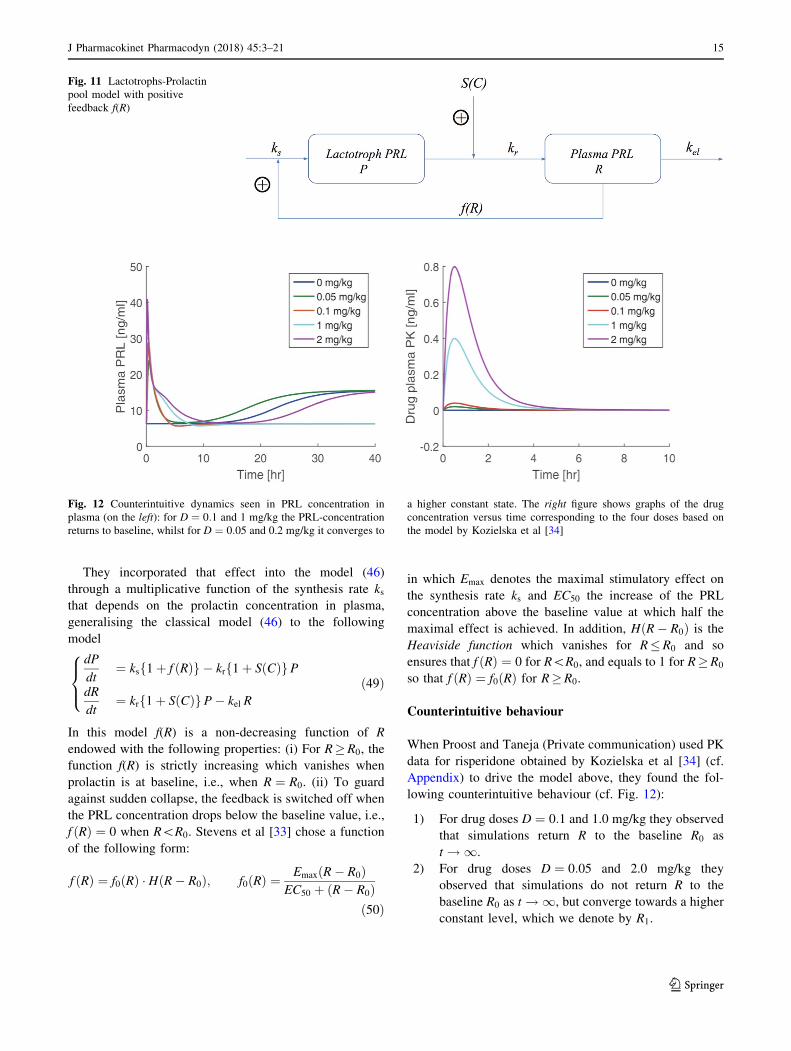
They incorporated that effect into the model (46)

through a multiplicative function of the synthesis rate ks

that depends on the prolactin concentration in plasma,

generalising the classical model (46) to the following

model

dP

dt¼ ksf1 þ f ðRÞg � krf1 þ SðCÞgP

dR

dt¼ krf1 þ SðCÞgP� kel R

8><

>:ð49Þ

In this model f(R) is a non-decreasing function of R

endowed with the following properties: (i) For RR0, the

function f(R) is strictly increasing which vanishes when

prolactin is at baseline, i.e., when R ¼ R0. (ii) To guard

against sudden collapse, the feedback is switched off when

the PRL concentration drops below the baseline value, i.e.,

f ðRÞ ¼ 0 when R\R0. Stevens et al [33] chose a function

of the following form:

f ðRÞ ¼ f0ðRÞ � HðR� R0Þ; f0ðRÞ ¼EmaxðR� R0Þ

EC50 þ ðR� R0Þð50Þ

in which Emax denotes the maximal stimulatory effect on

the synthesis rate ks and EC50 the increase of the PRL

concentration above the baseline value at which half the

maximal effect is achieved. In addition, HðR� R0Þ is the

Heaviside function which vanishes for R�R0 and so

ensures that f ðRÞ ¼ 0 for R\R0, and equals to 1 for RR0

so that f ðRÞ ¼ f0ðRÞ for RR0.

Counterintuitive behaviour

When Proost and Taneja (Private communication) used PK

data for risperidone obtained by Kozielska et al [34] (cf.

Appendix) to drive the model above, they found the fol-

lowing counterintuitive behaviour (cf. Fig. 12):

1) For drug doses D ¼ 0:1 and 1.0 mg/kg they observed

that simulations return R to the baseline R0 as

t ! 1.

2) For drug doses D ¼ 0:05 and 2.0 mg/kg they

observed that simulations do not return R to the

baseline R0 as t ! 1, but converge towards a higher

constant level, which we denote by R1.

Fig. 11 Lactotrophs-Prolactin

pool model with positive

feedback f(R)

Fig. 12 Counterintuitive dynamics seen in PRL concentration in

plasma (on the left): for D ¼ 0:1 and 1 mg/kg the PRL-concentration

returns to baseline, whilst for D ¼ 0:05 and 0.2 mg/kg it converges to

a higher constant state. The right figure shows graphs of the drug

concentration versus time corresponding to the four doses based on

the model by Kozielska et al [34]

J Pharmacokinet Pharmacodyn (2018) 45:3–21 15

123

3) The PK is fast, in that the half-life of drug in the

central compartment is around 1 h, whilst the time

for R to reach R0 is about 10 h and to reach R1 is

around 40 h.

This suggests that, (i) when CðtÞ � 0, there exists besides

the baseline R0 an additional steady state R1 [R0, and (ii)

the drug dependence of the dynamics is not monotone and

quite sensitive to drug dose. For practical situations this is

very critical so that it is important to find the reasons for

this behaviour.

In order to understand these phenomena it is necessary

to study the mathematical properties of the model (49) with

positive feedback function (50) more closely. That will be

done in the next subsection.

Mathematical analysis

To simplify the equations and reduce the number of

parameters, we introduce dimensionless variables. To this

end we scale P and R by their respective baseline values

and time by 1=kel and put:

x ¼ P

P0

; y ¼ R

R0

; s ¼ kel t ð51Þ

Introducing these variables into the system (49) and the

feedback function f(R) we obtain

dx

ds¼ a 1 þ uðyÞ � wðsÞ xf g

dy

ds¼ wðsÞ x� y

8><

>:a ¼ kr

kel

ð52Þ

where wðsÞ ¼ 1 þ SðCðtÞÞ and

uðyÞ ¼ bðy� 1Þcþ ðy� 1Þ � Hðy� 1Þ; b ¼ Emax;

c ¼ EC50

R0

ð53Þ

Stationary solutions

Suppose that the drug concentration is constant, i.e.

CðtÞ � C 0, and wðsÞ � w ¼ SðCÞ. Then, by (52) a sta-

tionary solution ðx; yÞ satisfies the pair of equations

1 þ uðyÞ ¼ w � x and w � x ¼ y

Substituting the second equation into the first yields the

following equation for y:

1 þ bðy� 1Þcþ ðy� 1Þ ¼ y ð54Þ

This is a quadratic equation in y which has the roots:

y0 ¼ 1 and y1 ¼ 1 þ b� c ð55Þ

Plainly, y0 corresponds to R0, the baseline in the absence of

positive feedback. However y1 corresponds to a new sta-

tionary solution which is introduced by the positive feed-

back, denoted by R1.

It is illustrative to follow the dynamics of the system in

what one may refer to as the state space, the (x, y)-plane in

which the state, defined by x and y, travels. It is often called

the Phase plane and the trajectory, traced by the concen-

tration pair (x(t), y(t)), is called the Orbit. Plainly, at each

point (x, y) in this plane the velocity vector q ¼ðdx=ds; dy=dsÞ can be computed from the system (52).

States at which x increases with time ðdx=ds[ 0Þ and

where x decreases with time ðdx=ds\0Þ are separated by

curves Cx where dx=ds ¼ 0. Similarly, Cy separates states

where y increases, respectively decreases. The curves Cx

and Cy are called the Null clines. Clearly, the stationary

states are located at the points where Cx and Cy intersect.

When C ¼ 0, then by the system (52), the null clines are

given by

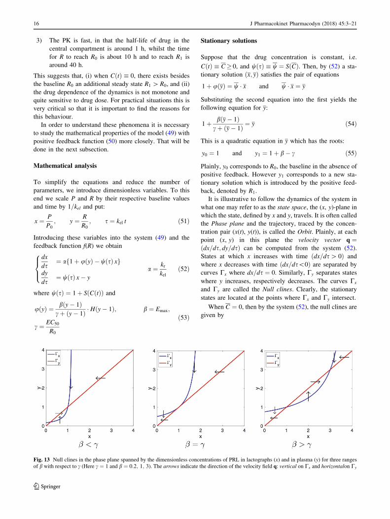
Fig. 13 Null clines in the phase plane spanned by the dimensionless concentrations of PRL in lactographs (x) and in plasma (y) for three ranges

of b with respect to c (Here c ¼ 1 and b ¼ 0:2; 1; 3). The arrows indicate the direction of the velocity field q: vertical on Cx and horizontalon Cy

16 J Pharmacokinet Pharmacodyn (2018) 45:3–21

123

Cx : y ¼ x and Cy : y ¼ 1 þ cðx� 1Þb� ðx� 1Þ ;

ðx 6¼ bþ 1Þð56Þ

These null clines are shown in Fig. 13 for c ¼ 1 and b ¼0:2; 1:0 and 3. Notice that Cy is fixed and Cx moves to the

right and up as b increases. As predicted by eq. (55), we

see that the corresponding steady states are, besides

ðx0; y0Þ ¼ ð1; 1Þ: ðx1; y1Þ ¼ ð0:2; 0:2Þ when b ¼ 0:2, and

ðx1; y1Þ ¼ ð3; 3Þ when b ¼ 3.

The null clines are very helpful in determining various

aspects of the dynamics of the system, such as (i) the sta-

bility of the steady states, (ii) the large-time behaviour of

orbits: e.g. where they go to and how they approach the

stable steady states and (iii) identification of invariant

regions, i.e., regions in the plane which trap orbits. Thus,

the arrows in Fig. 13 suggest that when the positive feed-

back is small, i.e., when b ¼ Emax is small, then ðx0; y0Þ ¼ð1; 1Þ is stable because all the arrows point towards it.

However, when the positive feedback becomes stronger,

and specifically, when b becomes larger than c, then

ðx0; y0Þ loses its stability and arrows point to ðx1; y1Þ.When the parameters in the system explicitly depend on

time, the situation is more complex. In the system (52) the

parameters are all constants except the coefficient wðsÞwhich depends on s. However, since CðtÞ ! 0 very

quickly (cf. Fig. 12, right panel), for most of the orbit we

may put C ¼ 0, and hence w ¼ 1, after a brief initial

period.

The specific parameter values employed for the system

(52) by Stevens et al [33] are given in Table 4.

They yield for the dimensionless constants: a ¼ 0:10,

b ¼ 3:47 and c ¼ 1:99. Thus, for the data used in [33] we

conclude that b[ c, so that the right-hand graph in Fig. 13

applies. For the baseline we obtain R0 ¼ 6:24 ng mL-1

and, using eq. (55), we obtain for the upper steady state

R1 ¼ R0 y1 ¼ R0ð1 þ b� cÞ ¼ 15:48 ng mL-1, in

agreement with the simulation shown in Fig. 12.

Summarising and rephrasing the observations made in

the simulations shown in Fig. 12 we can state that

RðtÞ ! R0 as t ! 1 when D ¼ 0:1&1:0 mg=kg;

RðtÞ ! R1 as t ! 1 when D ¼ 0:05&2:0 mg=kg

�

ð57Þ

and the question is, why the PRL concentration does not go

back to the baseline R0 for any initial dose. In the next

subsection we attempt to shed light on this observation.

Behaviour explained

In order to understand why the behaviour of the PRL-

concentration is so sensitive to the drug dose, we turn to the

phase plane and follow the orbit traced by the concentra-

tion pair (x, y) from its starting point ðx; yÞ ¼ ð1; 1Þ all the

way towards its limiting state ðx1; y1Þ. Specifically, we

wish to know when the orbit tends to ðx0; y0Þ and when to

ðx1; y1Þ, and how the drug dose D enters into this selection.

For simplicity we first study the dynamics of the system

(52) in the absence of a cut-off of the positive feedback.

For this case we show in Fig. 14 the orbits in the phase

plane for the drug doses D ¼ 0:05, 0.1, 1.0 and 2.0 mg/kg.

We observe in Fig. 14 that after a rapid introduction of

risperidone, all orbits leave the baseline ðx0; y0Þ ¼ ð1; 1Þmove up and to the left along an orbit which is initially

tangent to the line

‘ : y ¼ 1 þ 1

að1 � xÞ ¼ 1 þ 10 ð1 � xÞ: ð58Þ

After describing a big loop the orbits all return to a

neighbourhood of the baseline ðx0; y0Þ ¼ ð1; 1Þ from where

they started. However, because b[ c the baseline is

unstable and orbits move away from it, with the exception

of two orbits: one from above and one from below, which

tend towards ðx0; y0Þ. Orbits which pass above these

‘‘stable orbits’’ (cf. D ¼ 0:05 and 2 mg/kg) ultimately

converge towards the second equilibrium solution ðx1; y1Þ.Those which pass below (cf. D ¼ 0:1 and 1 mg/kg) leave

the first quadrant and they do this through the y-axis, below

the line y ¼ 1. This dichotomy is clearly demonstrated in

Fig. 14.

Table 4 Parameter values used

in [33]Parameter Value Unit Description

ks 35.7 ng mL-1 h-1 Synthesis rate PRL

kr 0.59 h�1 Release rate PRL

kel 5.7 h�1 Elimination rate PRL

Smax 25 – Maximal stimulation

SC50 0.08 ng mL-1 h Drug concentration when stimulation is half-maximal

Emax 3.47 – Maximal positive feedback

EC50 12.4 ng mL-1 h Value of R� R0 when feedback is half-maximal

J Pharmacokinet Pharmacodyn (2018) 45:3–21 17

123

Evidently, orbits entering the neighbourhood of ðx0; y0Þare very sensitive to small changes in paramater values or

to the drug dose: a small change may flip them to the other

side of the two stable orbits and change their subsequent

course dramatically. This is the phenomenon that Proost

and Taneja observed.

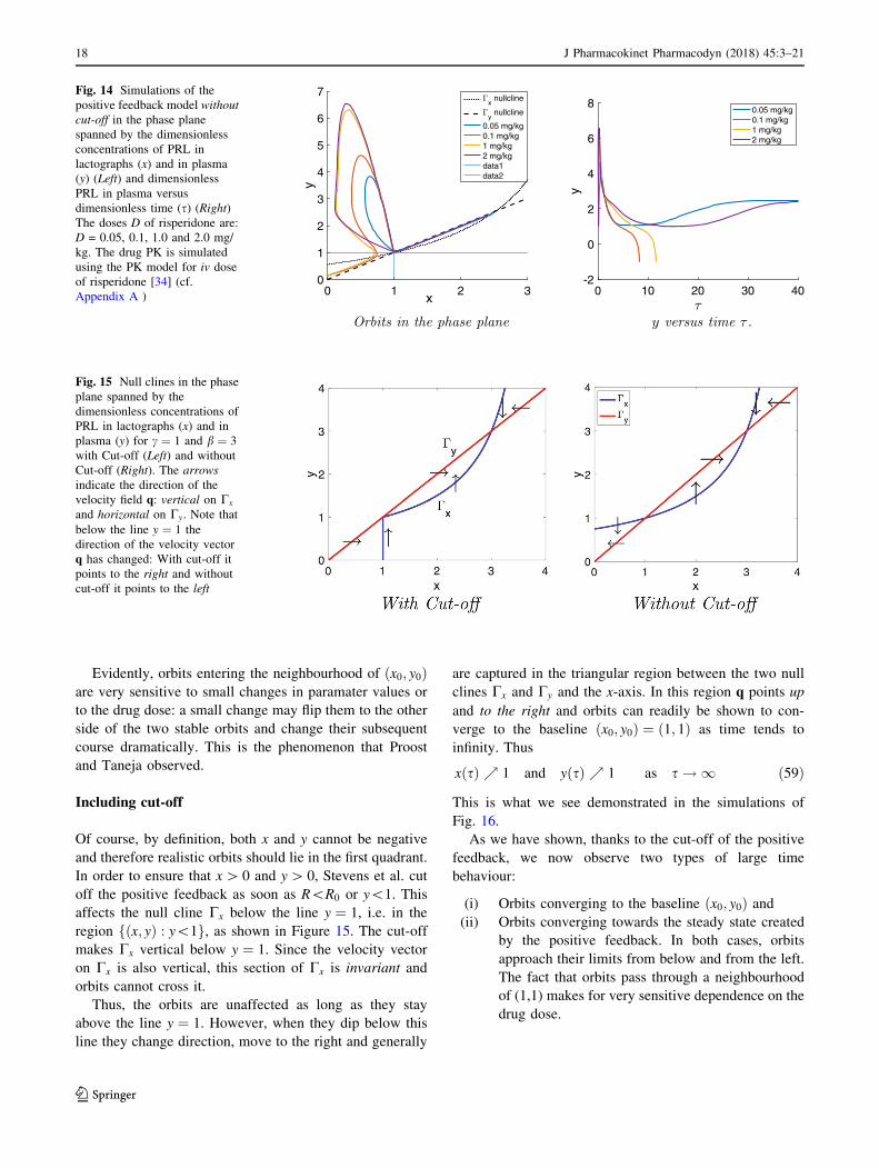
Including cut-off

Of course, by definition, both x and y cannot be negative

and therefore realistic orbits should lie in the first quadrant.

In order to ensure that x[ 0 and y[ 0, Stevens et al. cut

off the positive feedback as soon as R\R0 or y\1. This

affects the null cline Cx below the line y ¼ 1, i.e. in the

region fðx; yÞ : y\1g, as shown in Figure 15. The cut-off

makes Cx vertical below y ¼ 1. Since the velocity vector

on Cx is also vertical, this section of Cx is invariant and

orbits cannot cross it.

Thus, the orbits are unaffected as long as they stay

above the line y ¼ 1. However, when they dip below this

line they change direction, move to the right and generally

are captured in the triangular region between the two null

clines Cx and Cy and the x-axis. In this region q points up

and to the right and orbits can readily be shown to con-

verge to the baseline ðx0; y0Þ ¼ ð1; 1Þ as time tends to

infinity. Thus

xðsÞ % 1 and yðsÞ % 1 as s ! 1 ð59Þ

This is what we see demonstrated in the simulations of

Fig. 16.

As we have shown, thanks to the cut-off of the positive

feedback, we now observe two types of large time

behaviour:

(i) Orbits converging to the baseline ðx0; y0Þ and

(ii) Orbits converging towards the steady state created

by the positive feedback. In both cases, orbits

approach their limits from below and from the left.

The fact that orbits pass through a neighbourhood

of (1,1) makes for very sensitive dependence on the

drug dose.

Fig. 15 Null clines in the phase

plane spanned by the

dimensionless concentrations of

PRL in lactographs (x) and in

plasma (y) for c ¼ 1 and b ¼ 3

with Cut-off (Left) and without

Cut-off (Right). The arrows

indicate the direction of the

velocity field q: vertical on Cx

and horizontal on Cy. Note that

below the line y ¼ 1 the

direction of the velocity vector

q has changed: With cut-off it

points to the right and without

cut-off it points to the left

0 1 2 3x

0

1

2

3

4

5

6

7

y

x nullcline

y nullcline

0.05 mg/kg0.1 mg/kg1 mg/kg2 mg/kgdata1data2

0 10 20 30 40-2

0

2

4

6

8

y

0.05 mg/kg0.1 mg/kg1 mg/kg2 mg/kg

Orbits in the phase plane y versus time τ .

Fig. 14 Simulations of the

positive feedback model without

cut-off in the phase plane

spanned by the dimensionless

concentrations of PRL in

lactographs (x) and in plasma

(y) (Left) and dimensionless

PRL in plasma versus

dimensionless time (s) (Right)

The doses D of risperidone are:

D = 0.05, 0.1, 1.0 and 2.0 mg/

kg. The drug PK is simulated

using the PK model for iv dose

of risperidone [34] (cf.

Appendix A )

18 J Pharmacokinet Pharmacodyn (2018) 45:3–21

123

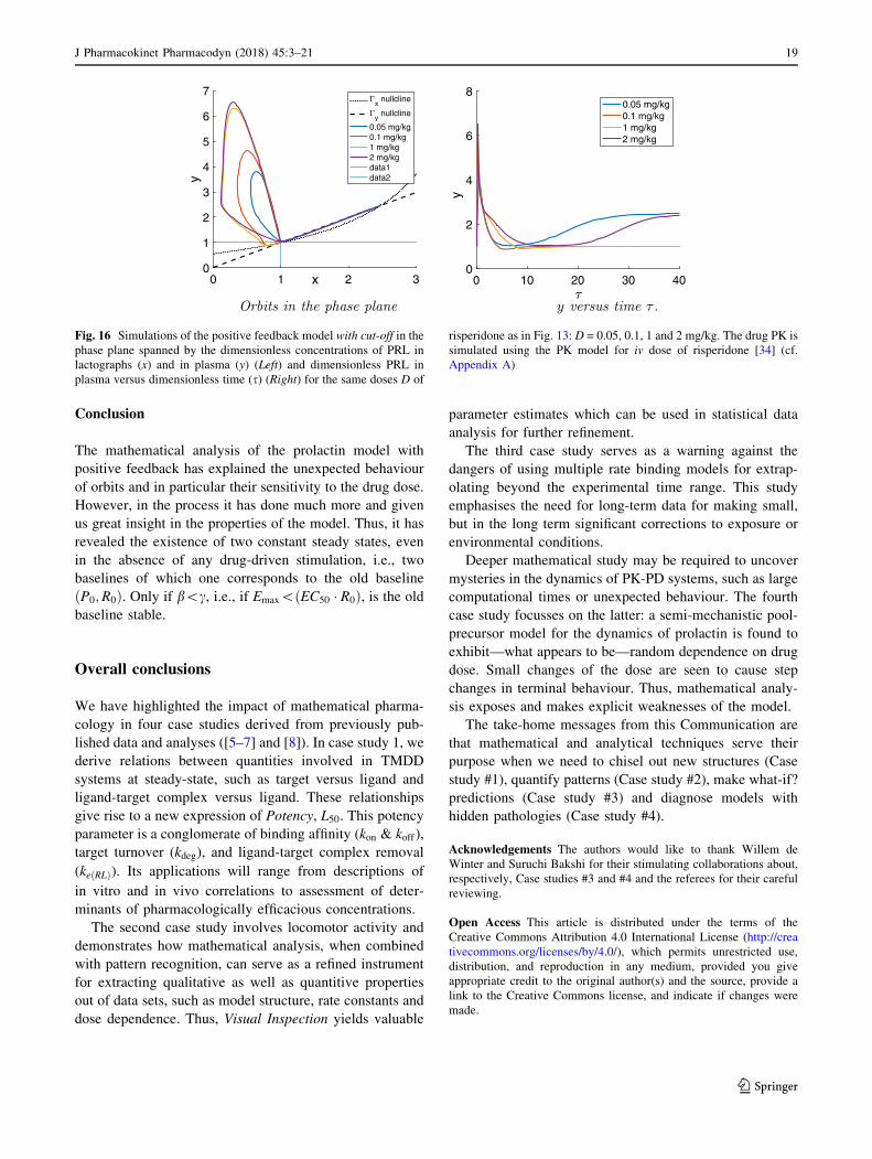
Conclusion

The mathematical analysis of the prolactin model with

positive feedback has explained the unexpected behaviour

of orbits and in particular their sensitivity to the drug dose.

However, in the process it has done much more and given

us great insight in the properties of the model. Thus, it has

revealed the existence of two constant steady states, even

in the absence of any drug-driven stimulation, i.e., two

baselines of which one corresponds to the old baseline

ðP0;R0Þ. Only if b\c, i.e., if Emax\ðEC50 � R0Þ, is the old

baseline stable.

Overall conclusions

We have highlighted the impact of mathematical pharma-

cology in four case studies derived from previously pub-

lished data and analyses ([5–7] and [8]). In case study 1, we

derive relations between quantities involved in TMDD

systems at steady-state, such as target versus ligand and

ligand-target complex versus ligand. These relationships

give rise to a new expression of Potency, L50. This potency

parameter is a conglomerate of binding affinity (kon & koff),

target turnover (kdeg), and ligand-target complex removal

(keðRLÞ). Its applications will range from descriptions of

in vitro and in vivo correlations to assessment of deter-

minants of pharmacologically efficacious concentrations.

The second case study involves locomotor activity and

demonstrates how mathematical analysis, when combined

with pattern recognition, can serve as a refined instrument

for extracting qualitative as well as quantitive properties

out of data sets, such as model structure, rate constants and

dose dependence. Thus, Visual Inspection yields valuable

parameter estimates which can be used in statistical data

analysis for further refinement.

The third case study serves as a warning against the

dangers of using multiple rate binding models for extrap-

olating beyond the experimental time range. This study

emphasises the need for long-term data for making small,

but in the long term significant corrections to exposure or

environmental conditions.

Deeper mathematical study may be required to uncover

mysteries in the dynamics of PK-PD systems, such as large

computational times or unexpected behaviour. The fourth

case study focusses on the latter: a semi-mechanistic pool-

precursor model for the dynamics of prolactin is found to

exhibit—what appears to be—random dependence on drug

dose. Small changes of the dose are seen to cause step

changes in terminal behaviour. Thus, mathematical analy-

sis exposes and makes explicit weaknesses of the model.

The take-home messages from this Communication are

that mathematical and analytical techniques serve their

purpose when we need to chisel out new structures (Case

study #1), quantify patterns (Case study #2), make what-if?

predictions (Case study #3) and diagnose models with

hidden pathologies (Case study #4).

Acknowledgements The authors would like to thank Willem de

Winter and Suruchi Bakshi for their stimulating collaborations about,

respectively, Case studies #3 and #4 and the referees for their careful

reviewing.

Open Access This article is distributed under the terms of the

Creative Commons Attribution 4.0 International License (http://crea

tivecommons.org/licenses/by/4.0/), which permits unrestricted use,

distribution, and reproduction in any medium, provided you give

appropriate credit to the original author(s) and the source, provide a

link to the Creative Commons license, and indicate if changes were

made.

0 1 2 3x0

1

2

3

4

5

6

7

y

x nullcline

y nullcline

0.05 mg/kg0.1 mg/kg1 mg/kg2 mg/kgdata1data2

0 10 20 30 400

2

4

6

8

y

0.05 mg/kg0.1 mg/kg1 mg/kg2 mg/kg

Orbits in the phase plane y versus time τ .

Fig. 16 Simulations of the positive feedback model with cut-off in the

phase plane spanned by the dimensionless concentrations of PRL in

lactographs (x) and in plasma (y) (Left) and dimensionless PRL in

plasma versus dimensionless time (s) (Right) for the same doses D of

risperidone as in Fig. 13: D = 0.05, 0.1, 1 and 2 mg/kg. The drug PK is

simulated using the PK model for iv dose of risperidone [34] (cf.

Appendix A)

J Pharmacokinet Pharmacodyn (2018) 45:3–21 19

123

Appendix

PK used by Kozielska et al [34]

Kozielsky et al used a simple two-compartment model

involving a central and a peripheral compartment in which

the drug-amounts were denoted by, respectively, Ac and Ap.

The drug entered the central compartment from a depot

which was supplied by an iv bolus dose.

dAd

dt¼ �kaAd

dAc

dt¼ kaAd �

CL

Vc

Ac �CLd

Vc

Ac þCLd

Vp

Ap

dAp

dt¼ CLd

Vc

Ac �CLd

Vp

Ap

8>>>>>>><

>>>>>>>:

ð60Þ

where ka denotes the first-order rate with which drug is

transported from the depot into the plasma compartment

CL the clearance from the plasma compartment and CLdthe distributional clearance between the plasma- and the

peripheral compartment. The volumes of the plasma- and

the peripheral compartment are denoted by Vc and Vp,

respectively. The PK parameter values used by Kozielska

et al are given in Table 5.

References

1. Woodcock J, Woosley R (2008) The FDA Critical Path Initiative

and its influence on new drug development. Annu Rev Med

59:1–12

2. Benson N, Cucurull-Sanchez L, Demin O, Smirnov S, Van der

Graaf P (2012) Reducing systems biology to practice in phar-

maceutical company research; selected case studies. Adv Syst

Biol 736:607–615

3. Fujioka A, Terai K, Itoh R, Aoki K, Nakamura T, Kuroda S,

Nishida E, Matsuda M (2006) Dynamics of the Ras/ERK MAPK

cascade as monitored by fluorescent probes. J Biol Chem

281:8917–8926

4. Courant R, Hilbert D (1962) Methods of mathematical physics,

vol 2. Interscience Publishers Inc., New York

5. Gabrielsson J, Peletier LA (2017) Pharmacokinetic steady-states

highlight interesting target-mediated disposition properties.

AAPS J 19:772–786. doi:10.1208/s12248-016-0031-y

6. Gabrielsson J, Peletier LA (2014) Dose-response-time data

analysis involving nonlinear dynamics, feedback and delay. Eur J

Pharm Sci 59:36–48

7. Peletier LA, de Winter W, Vermeulen A (2012) Dynamics of a

two-receptor binding model: how affinities and capacities trans-

late into long and short time behaviour and physiological corol-

laries. Discret Contin Dyn Syst Ser B 17:2171–2184

8. Bakshi S, de Lange EC, van der Graaf PH, Danhof M, Peletier

LA (2016) Understanding the behavior of systems pharmacology

models using mathematical analysis of differential equations:

prolactin modeling as a case study. CPT Pharmacomet Syst

Pharmacol 5:339–351. doi:10.1002/psp4.12098

9. Mager D, Jusko WJ (2001) General pharmacokinetic model for

drugs exhibiting target-mediated drug disposition. J Pharma-

cokinet Phamacodyn 28:507–532

10. Mager D, Krzyzanski W (2005) Quasi-equilibrium pharmacoki-

netic model for drugs exhibiting target-mediated drug disposition.

Pharm Res 22:1589–1596

11. Mager DE (2006) Target-mediated drug disposition and dynam-

ics. Biochem Pharmacol 72:1–10

12. Gibiansky L, Gibiansky E, Kakkar T, Ma P (2008) Approxima-

tions of the target-mediated drug disposition model and identifi-

ability of model parameters. J Pharmacokinet Pharmacodyn

35:573–591

13. Krippendorff BF, Kuester K, Kloft C, Huisinga W (2009) Non-

linear pharmacokinetics of therapeutic proteins resulting from

receptor mediated endocytosis. J Pharmacokinet Pharmacodyn

36:239–260

14. Peletier LA, Gabrielsson J (2009) Dynamics of target-mediated

drug disposition. Eur J Pharm Sci 38:445–464

15. Peletier LA, Gabrielsson J (2012) Dynamics of target-mediated

drug disposition: characteristic profiles and parameter identifi-

cation. J Pharmacokinet Pharmacodyn 39:429–451

16. Ma P (2012) Theoretical considerations of target-mediated drug

disposition models: simplifications and approximations. Pharm

Res 29:866–882

17. Dua P, Hawkins E, Van der Graaf PH (2015) A tutorial on target-

mediated drug disposition (TMDD) models. CPT Pharmacomet-

rics Syst Pharmacol 4:324–337. doi:10.1002/psp4.41

18. Cao Y, Jusko WJ (2014) Incorporating target-mediated drug

disposition in a minimal physiologically-based pharmacokinetic

model for monoclonal antibodies. J Pharmacokinet Pharmacodyn

41:375–387

19. Levy G (1964) Relationship between elimination rate of drugs

and rate of decline of their pharmacologic effects. J Pharm Sci

53:342–343

20. Levy G (1966) Kinetics of pharmacological effects. Clin Phar-

macol Ther 7:362–372

21. Smolen VF (1971) Quantitative determination of drug bioavail-

ability and biokinetic behavior from pharmacological data for

ophtalmic and oral administration of a mydriatic drug. J Pharm

Sci 60:354–363

22. Uehlinger DE, Gotch FA, Sheiner LB (1992) A pharmacody-

namic model of erythropoietin therapy for uremic anemia. Clin

Pharmacol Ther 51:76–89

23. Port RE, Ding RW, Fies T, Scharer K (1998) Predicting the time

course of haemoglobin in children treated with erythropoietin for

Table 5 PK parameters used by

Kozielska et al [34]Parameter Estimate Units Description

ka 2.84 L hr�1 Influx rate from depot

CL 1.62 L hr�1�kg�1 Clearance

Vc 1.29 L kg�1 Volume central compartment

CLd 0.0882 L hr�1�kg�1 Distributional clearance

Vp 1.29 L kg�1 Volume peripheral compartment

20 J Pharmacokinet Pharmacodyn (2018) 45:3–21

123

renal anaemia. Br J Clin Pharmacol. 46(5):461–466, ISSN

03065251. 10.1046/j.1365-2125.1998.00797.x

24. Gruwez B, Dauphin A, Tod M (2005) A mathematical model for

paroxetine antidepressant effect time course and its interaction

with pindolol. J Pharmacokinet Phar 32:663–683. doi:10.1007/

s10928-005-0006-6

25. Berangere Gruwez B, Marie-France Poirier M-F, Alain Dauphin

A, Jean-Pierre Olie, Tod M (2007) A kinetic-pharmacodynamic

model for clinical trial simulation of antidepressant action:

application to clomipramine-lithium interaction. Contemp Clin

Trials. 28:276–87. ISSN 1551-7144. http://www.ncbi.nlm.nih.

gov/pubmed/17059901

26. Lange MR, Schmidli H (2014) Optimal design of clinical trials

with biologics using dose-time-response models. Stat Med

33:5249–5264. doi:10.1002/sim.6299

27. Lange MR, Schmidli H (2015) Analysis of clinical trials with

biologics using dose-time-response models. Stat Med

34:3017–3028. doi:10.1002/sim.6551

28. Andersson R, Jirstrand M, Peletier LA, Chappell MJ, Evans ND,

Gabrielsson J (2016) Dose-response-time modelling: second-

generation turnover model with integral feedback control. Eur J

Pharm Sci 81:189–200

29. van Rossum JM, Van Koppen AT (1968) Kinetics of psycho-

motor stimulus drug action. Eur J Pharmacol 2:405–408

30. Michaelis L, Menten ML (1913) Die Kinetik der Invertin-

wirkung. Biochem Z 49:333–369

31. Snoeck E, Jacqmin Ph, van Peer A, Danhof M (1999) A com-

bined specific target site binding and pharmacokinetic model to

explore the non-linear disposition of draflazine. J Pharmacokinet

Biopharm 27:257–281

32. Peletier LA, de Winter W (2017) Impact of saturable distribution

in compartmental PK models: dynamics and practical use.

J Pharmacokinet Pharmacodyn 44:1–16. doi:10.1007/s10928-

016-9500-2

33. Stevens J, Ploeger BA, Hammarlund-Udenaes M, Osswald G, van

der Graaf PH, Danhof M, de Lange ECM (2012) Mechanism-

based PK-PD model for the prolactin biological system response

following an acute dopamine inhibition challenge: quantitative

extrapolation to humans. J Pharmacokinet Pharmacodyn

39:463–477

34. Kozielska M, Johnson M, Reddy VP, Vermeulen A, Li C,

Grimwood S, de Greef R, Groothuis GMM, Danhof M, Proost JH

(2012) Pharmacokinetic-pharmacodynamic modeling of the D(2)

and 5-HT(2A) receptor occupancy of risperidone and paliperi-

done in rats. Pharmaceutic Res 29(7):1932–1948

35. Movin-Osswald G, Hammarlund-Udenaes M (1995) Prolactin

release after remoxipride by an integrated pharmacokinetic

pharmacodynamic model with intra- and interinduvidual aspects.

J Pharmacol Exp Ther 274:921–927

36. Ekblad EB, Licko V (1984) A model eliciting transient response.

Am J Physiol 246:R114–21

37. Ekblad EB, Licko V (1987) Conservative and nonconservative

inhibitors of gastric acid secretion. Am J Physiol Gastrointest

Liver Physiol 253(3):G359–368

38. Sharma A, Ebling WF, Jusko WJ (1998) Precursor-dependent

indirect pharmacodynamic response model for tolerance and

rebound phenomena. J Pharm Sci 87:1577–1584

39. Friberg LE, Vermeulen AM, Petersson KJF, Karlsson MO (2009)

An agonistantagonist interaction model for prolactin release fol-

lowing risperidone and paliperidone treatment. Clin Pharm Ther

85(4):408–417

J Pharmacokinet Pharmacodyn (2018) 45:3–21 21

123