Impact of Low Rotational Inertia onPower System Stability and Operation

Andreas Ulbig, Theodor S. Borsche, Göran Andersson

ETH Zurich, Power Systems LaboratoryPhysikstrasse 3, 8092 Zurich, Switzerlandulbig | borsche | andersson @ eeh.ee.ethz.ch

Abstract: Large-scale deployment of Renewable Energy Sources (RES) has led to significantgeneration shares of variable RES in power systems worldwide. RES units, notably inverter-connected wind turbines and photovoltaics (PV) that as such do not provide rotational inertia,are effectively displacing conventional generators and their rotating machinery. The traditionalassumption that grid inertia is sufficiently high with only small variations over time is thus notvalid for power systems with high RES shares. This has implications for frequency dynamicsand power system stability and operation. Frequency dynamics are faster in power systems withlow rotational inertia, making frequency control and power system operation more challenging.This paper investigates the impact of low rotational inertia on power system stability andoperation, contributes new analysis insights and offers impact mitigation options.

Keywords: Rotational Inertia, Power System Stability, Grid Integration of Renewables

1. INTRODUCTION

Traditionally, power system operation is based on theassumption that electricity generation, in the form of ther-mal power plants, reliably supplied with fossil or nuclearfuels, or hydro plants, is fully dispatchable, i.e. control-lable, and involves rotating synchronous generators. Viatheir stored kinetic energy they add rotational inertia,an important property of frequency dynamics and stabil-ity. The contribution of inertia is an inherent and cru-cial feature of rotating synchronous generators. Due toelectro-mechanical coupling, a generator’s rotating massprovides kinetic energy to the grid (or absorbs it fromthe grid) in case of a frequency deviation ∆f . The kineticenergy provided is proportional to the rate of change offrequency ∆f (Kundur, 1994). The grid frequency f isdirectly coupled to the rotational speed of a synchronousgenerator and thus to the active power balance. Rotationalinertia, i.e. the inertia constant H, minimizes ∆f in caseof frequency deviations. This renders frequency dynamicsmore benign, i.e slower, and thus increases the availableresponse time to react to fault events such as line losses,power plant outages or large-scale set-point changes ofeither generation or load units.

Maintaining the grid frequency within an acceptable rangeis a necessary requirement for the stable operation ofpower systems. Frequency stability and in turn also sta-ble operation both depend on the active power balance,meaning that the total power in-feed minus the total loadconsumption (including system losses) is kept close tozero. In normal operation small variations of this balanceoccur spontaneously. Deviations from its nominal value f0,e.g. 50 Hz or 60 Hz depending on region, should be keptsmall, as damaging vibrations in synchronous machinesand load shedding occur for larger deviations. This can

influence the whole power system, in the worst case endingin fault cascades and black-outs. Low levels of rotationalinertia in a power system, caused in particular by highshares of inverter-connected RES, i.e. wind turbine andPV units that normally do not provide any rotationalinertia, have implications on frequency dynamics. Theyare becoming faster in power systems with low rotationalinertia. This can lead to situations in which traditionalfrequency control schemes become too slow with respectto the disturbance dynamics for preventing large frequencydeviations and the resulting consequences. The loss ofrotational inertia and its increasing time-variance lead tonew frequency instability phenomena in power systems.Frequency and power system stability may be at risk.

An exemplary analysis of the German power system showsthe relevance of the above mentioned trends. Throughoutthe year 2012 there have been several occasions hours inwhich around 50% of overall load demand was covered bywind&PV units. The regional inertia within the Germanpower system dropped to significantly lower levels thanusual due to the temporary lack of dispatched conven-tional generators and their rotating machinery. With theincrease of inverter-connected RES generation, low inertiasituations will become more widespread and with it fasterfrequency dynamics and the associated operational risks.

The remainder of this paper is organized as follows: Sec-tion 2 discusses the rapid large-scale deployment of RESgeneration in many countries and the arising challengesfor power system operation. Section 3 explains rotationalinertia in more detail and assesses to what extent inverter-connected generation units reduce inertia and render ittime-variant. This is followed by an analysis of the impactsof reduced inertia on power system stability in Section 4and power system operation in Section 5. Finally, a con-clusion and an outlook are given in Section 6.

Preprints of the 19th World CongressThe International Federation of Automatic ControlCape Town, South Africa. August 24-29, 2014

Copyright © 2014 IFAC 7290

2. IMPACTS OF RISING RENEWABLE ENERGYSHARES FOR POWER SYSTEM OPERATION

Facing the challenge of having to reduce CO2 emissionsdue to climate change concerns as well as security ofsupply issues of fossil fuels, many countries nowadays arecommitted to increasing the share of renewable energysources (RES) in their electric power systems.

Large-scale deployment of RES generation, notably inthe form of wind turbines and PV units, ranging fromsmall and highly distributed units, e.g. roof-top PV witha rating of a few kilowatts (kW), to large units, e.g. largePV and wind farms with hundreds of megawatts (MW),has led to significant generation shares of variable RESpower in-feed in power systems worldwide. RES capac-ity comprised about 25% of total global power genera-tion capacity and produced an estimated 20.3% of globalelectricity demand by by year-end 2011. Although mostRES electricity is still provided by hydro power (15 %)other renewables (5.3 %) are on the rise. Of the world’stotal generation capacity estimated at 5360GWel by year-end 2011, wind power made up 238GWel (4.4 %), solarPV 70GWel (1.3 %) whereas Concentrating Solar ThermalPower (CSP) only contributed 1.8GWel (0.03 %). In theEuropean Union (EU-28), with a total generation capac-ity of around 870GWel, wind power made up 94GWel(10.8 %) and solar PV 51GWel (5.9 %) (REN21, 2012).

In Germany, the RES share of electricity generation in-creased from 4.7% of net load demand in 1998 to morethan 20% in 2012. RES generation capacity is dominatedby wind, PV and hydro generation with an absolute shareof net load demand of 8.3%, 5.0% and 3.9%, respectively,in 2012. The remainder was made up of biomass, land-filland bio gas generation (3–4%) (BMU, 2013).

Due to the rising RES shares, the number of hours per yearin which RES in-feed makes up a large part or the majorityof power production in a grid region is also increasing. Thisis illustrated for the case of Germany in Fig. 1 (a)–(b).There, the power dispatch situation of wind&PV units andconventional generation in the German power system is il-lustrated for December 2012 (31 days). Also, the histogram

of the total inverter-connected RES in-feed, i.e. wind&PV,as a share of the total load demand in Germany is givenfor the full year 2012. In this particular year the shareof inverter-connected RES units often reached significantlevels: a share of 30% or more was reached for 495 hoursa year (5.6%), 40% or more for 221 hours (2.5%) and arecord 50% for 0.75 hours (0.009%), respectively.

3. TIME-VARIANCE OF GRID INERTIA

In the following the basic modeling concepts for rotationalinertia in power systems as well as synchronous powersystems in general are presented.

3.1 Modeling Inertial Response

Following a frequency deviation, kinetic energy stored inthe rotating masses of the generator system is released,rendering power system frequency dynamics slower and,hence, easier to regulate. The rotational energy is given as

Ekin =1

2J(2πfm)2 , (1)

with J as the moment of inertia of the synchronousmachine and fm the rotating frequency of the machine.The inertia constant H for a synchronous machine isdefined by

H =Ekin

SB=J(2πfm)2

2SB, (2)

with SB as the rated power of the generator and H de-noting the time duration during which the machine cansupply its rated power solely with its stored kinetic energy.Typical values for H are in the range of 2–10 s (Kundur,1994, Table 3.2). The classical swing equation, a well-known model representation for synchronous generators,describes the inertial response of the synchronous genera-tor as the change in rotational frequency fm (or rotationalspeed ωm = 2π ·fm) of the synchronous generator followinga power imbalance as

Ekin = J(2π)2fm · fm =2HSB

fm· fm = (Pm − Pe) , (3)

with Pm as the mechanical power supplied by the generatorand Pe as the electric power demand.

Fig. 1. (a) Power Dispatch Situation in German Power System (December 2012). (b) Histogram of Inverter-ConnectedPower In-feed Shares in German Power System (full-year 2012).

19th IFAC World CongressCape Town, South Africa. August 24-29, 2014

7291

Noting that frequency excursions are usually small de-viations around the reference value, we replace fm byf0 and Pm by Pm0, and complete the classical SwingEquation by adding frequency-dependent load damping, aself-stabilizing property of power systems, by formulating

fm = − f0

2HSBDloadfm +

f0

2HSB(Pm, 0 − Pe) . (4)

Here f0 is the reference frequency and Dload denotes thefrequency-dependent load damping constant. Pm, 0 is thenominally scheduled mechanical generator power. Notethat a concurrent and (more) often used definition of loaddamping is k = 1

Dload. The high share of conventional

generators is translated into a large rotational inertiaof the here presented interconnected power system. Thehigher the inertia constant H of the system, the slower andmore benign are grid frequency dynamics. For identicalpower imbalance faults frequency deviations fm and theirderivative fm will become smaller.

With an increasing penetration of inverter-connectedpower units, the rotational inertia of power systems isreduced and becomes highly time-variant as wind&PVshares are fluctuating heavily throughout the year. Thisis notably a concern for small power networks, e.g. islandor micro grids, with a high share of generation capacitynot contributing any inertia as was discussed and illus-trated, for example, in Tielens and Van Hertem (2012).Frequency stabilization becomes thus more difficult. Ap-propriate adaptations of grid codes are needed.

3.2 Aggregated Swing Equation Model

Modeling interconnected power systems, i.e. different ag-gregated generator and load nodes that are connected viatie-lines, can be realized in a similar fashion as modelingindividual generators. Reformulating the classical SwingEquation (Eq. 4) for a power system with n generators,j loads and l connecting tie-lines, leads to the so-calledAggregated Swing Equation (ASE) (Kundur, 1994)

f = − f0

2HSBDloadf +

f0

2HSB(Pm − Pload − Ploss) , (5)

with

f =

∑ni=1Hi SB,i fi∑ni=1Hi SB,i

, SB =

n∑i=1

SB,i , H =

∑ni=1HiSB,i

SB,

Pm =

n∑i=1

Pm,i , Pload =

j∑i=1

Pload,i , Ploss =

l∑i=1

Ploss,i .

Here the term f is the Center of Inertia (COI) gridfrequency, H the aggregated inertia constant of the ngenerators, SB the total rated power of the generators,Pm the total mechanical power of the generators, Ploadthe total system load of the grid and Ploss the totaltransmission losses of the l lines making up the gridtopology and f0 = 50 Hz. The term Dload is the frequencydamping of the system load, which is assumed here to beconstant and uniform. All power system parameters aregiven in Table 1.

The ASE model (Eq. 5) is valid for a highly meshed grid,in which all units can be assumed to be connected to thesame grid bus, representing the Center of Inertia of thegiven grid. Since load-frequency disturbances are normallyrelatively small, linearized swing equations with ∆fi =fi − f0 can be used. Considering the system change (∆)before and after a disturbance, the relative formulation ofthe ASE, assuming that ∆Ploss = 0, is

∆f = − f0

2HSBDload∆f +

f0

2HSB(∆Pm −∆Pload) . (6)

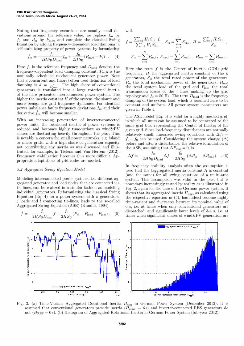
In frequency stability analysis often the assumption isused that the (aggregated) inertia constant H is constant(and the same) for all swing equations of a multi-areasystem. This assumption was valid in the past but isnowadays increasingly tested by reality as is illustrated inFig. 2, again for the case of the German power system. Itshows that its aggregated inertia Hagg, as calculated usingthe respective equation in (5), has indeed become highlytime-variant and fluctuates between its nominal value of6 s, i.e. at times when only conventional generators aredispatched, and significantly lower levels of 3-4 s, i.e. attimes when significant shares of wind&PV generation are

Fig. 2. (a) Time-Variant Aggregated Rotational Inertia Hagg in German Power System (December 2012). It isassumed that conventional generators provide inertia (Hconv = 6 s) and inverter-connected RES generators donot (HRES = 0 s). (b) Histogram of Aggregated Rotational Inertia in German Power System (full-year 2012).

19th IFAC World CongressCape Town, South Africa. August 24-29, 2014

7292

deployed. Note that the lowest level of rotational inertiaof this year was reached during the Christmas vacation inwhich demand levels were at their lowest (in Dec. 2012),while notably wind power in-feed was unusually high. Thehistogram for the full year 2012 reveals that inertia levelsdrop to rather low levels for a significant part of the time:Hagg was below 4 s for 293 hours (3.3%) and below 3.5 sfor 57 h (0.65%) of the time. The qualitative results of thisexample are valid also for the inertia situation in othercountries with high RES shares.

As this section and the previous one show, coping with thefluctuating electricity production from variable RES, i.e.wind turbines and PV, is a challenge for the operation ofelectric power systems in many aspects. The increasingshare of inverter-based power generation and the asso-ciated displacement of usually large-scale and fully con-trollable generation units and their rotational masses, inparticular has the following consequences:

(1) The pool of suitable conventional power plants forproviding traditional control reserve power is signifi-cantly diminished.

(2) The rotational inertia of power systems becomesmarkedly time-variant and is reduced, often non-uniformly within the grid topology, as will be pre-sented in the following section.

4. IMPACT OF LOW ROTATIONAL INERTIA ONPOWER SYSTEM STABILITY

Frequency dynamics of single-area as well as multi-areapower systems are usually modeled and analyzed employ-ing the Swing Equation approach introduced in Section 3.

It is known that frequency dynamics for a system withn areas can become chaotic in case n ≥ 3; confer to Kopelland Washburn (1982), Chiang et al. (1987) or Berggrenand Andersson (1993) for more details. Analyzing thestability properties of swing equation models of powersystems constituted a sizeable research stream in the 1980sand early 1990s. Although the analysis presented backthen assumed that rotational inertia constants could varyfrom one grid region to another, its time-variance causedby massive inverter-connected RES in-feed was not consid-ered at the time as only very few wind&PV units existed.

The following analyses use a three-area power system thatwas simplified to a two-area model, as the reference voltageangle and frequency of the third grid area are kept atzero, i.e. δ3 = 0, ω3 = 0. The modeling is based on theSwing Equation approach and follows the line of thoughtpresented in the work of Chiang et al. (1987):

δ1 = ω1 (7)

δ2 = ω2

ω1 =1

M1[∆P1 − k1ω1 − V1V2B2 sin(δ1 − δ2)

− V1V3B3 sin(δ1 − δ3)]

ω2 =1

M2[∆P2 − k2ω2 − V2V1B1 sin(δ2 − δ1)

− V2V3B3 sin(δ2 − δ3)] .

Here the voltage levels Vi are assumed to be nominal,i.e. 1 p.u. The specifications of all parameters are given inTable 1. Also, the familiar terms for rotational inertia andpower deviations are linked with the previous equationsintroduced in Section 3 via

Mi =2HiSBi

2πf0= Jiωi and ∆Pi = (∆Pm −∆Pload) .

(8)For the sake of simplicity in presentation and for easiercomparison with the related work previously mentioned,we use in this section the inertia constants Mi insteadof Hi and the angular frequency ωi = 2πfi, given inrad/s, instead of using directly the frequency fi. FromEq. 7 one can analytically deduce that the inertia constantMi mitigates the impact of shocks such as sudden powerfaults ∆Pi on the angular frequency ωi since ωi ∼

(∆Pi

Mi

).

Also the damping coefficient ki has a stabilizing effecton ωi since ωi ∼

(− kiMi· ωi). The achieved stabilizing

effect depends, however, also on the ratio of(kiMi

). Both

the values of the inertia constant Mi and the dampingcoefficient ki are thus vital for power system stability.

In Chiang et al. (1987), the stability region V (x) of asimplified two-area power system around the origin wasexplicitly calculated and shown. We show in the followingthat the size and form of this stability region are directlyshaped by the choice of the terms Mi and ki. Theydetermine how well shocks are absorbed by a power systemand how close they drive the system towards the stabilityboundary ∂V (x). We have calculated the stability regionof the two-area system given by Eq. 7 for different choicesof Mi and ki. The results are shown in Fig. 3. As wasstated by Chiang et al. (1987), the stability region (shownin green) is unbounded and centered at the origin.

The stability region extends along two axes: the frequencyangle difference x1 := δ1 − δ2 and the frequency deviation

Fig. 3. Unbounded Stability Region of Two-Area Systemfor Different Inertia Mi and Damping ki (clock-wise).(a) Mi = M0, ki = k0, (b) Mi = 2 ·M0, ki = k0,(c)Mi = 0.5·M0, ki = 2·k0, (d)Mi = M0, ki = 2·k0.

19th IFAC World CongressCape Town, South Africa. August 24-29, 2014

7293

−0.2 0 0.2 0.4

−0.5

−0.2

0

0.2

0.5

x1 = δ1 − δ2

x2

=ω1−ω2

(a) H1 = 6 s

−0.2 0 0.2 0.4

x1 = δ1 − δ2

(b) H1 = 3 s

−0.2 0 0.2 0.4

x1 = δ1 − δ2

(c) H1 = 3 s, high damping

FaultRecovery

−0.2 0 0.2 0.4 0.6 0.8

−0.5

−0.2

0

0.2

0.5

δ1(t) [◦]

∆f1(t

)[H

z]

−0.2 0 0.2 0.4 0.6 0.8

δ1(t) [◦]

−0.2 0 0.2 0.4 0.6 0.8

δ1(t) [◦]

FaultRecovery

Fig. 4. Upper Plots: Phase-Plot of Two-Area System, Lower Plots: Phase-Plot of Grid Area I.(a) High Inertia and Low Damping in Grid Area I (H1 = H2 = 6s, k1 = k2 = 0.015).(b) Low Inertia and Low Damping in Grid Area I (H1 = 3s, H2 = 6s, k1 = k2 = 0.015).(c) Low Inertia and High Damping in Grid Area I (H1 = 3s, H2 = 6s, k1 = 0.045, k2 = 0.015).

x2 := f1 − f2 = 12π (ω1 − ω2). It is of critical importance

that this region is sufficiently large along the x2-axis, sinceany power fault event happening in a grid region i itself(∆Pi) or imported via the power lines from neighboringgrid regions j (∆P tie

i,j ) has a direct impact on ωi. Rotationalinertia is beneficial in reducing the direct impact of ∆Pion ωi, i.e. the excursion of the system state from theorigin along the x1-axis, whereas the damping coefficientki is good for increasing the size of the stability regionalong the x2-axis. As we will show in the next section,additional damping can be emulated by fast primaryfrequency control.

Illustrations of the effect of different values ofMi and ki aregiven for the two-area power system in the form of phase-plots (Fig. 4 – upper plots). Here, the impact of a shock,i.e. a power deviation in Grid Area I given by ∆Pi, is simu-lated. This results in an excursion of the system state awayfrom the origin to a new equilibrium point on the x1-axis,as (trajectory shown in magenta). After a while, the powerfault is cleared and the system then moves back towardsthe origin (trajectory shown in green). Depending on thechoice of parametersMi and ki the critical excursion of thesystem’s phase trajectory along the x2-axis is smaller (forlarge values ofMi and ki) or larger (for small values ofMi

and ki). Note that frequency deviations ∆f of more than±0.5Hz may cause considerable generation tripping.Theadditional phase-plot trajectories of Grid Area I, ( Fig. 4 –lower plots), show that this critical limit is indeed violatedin one instance (Fig. 4 – bottom, center).

5. IMPACT OF LOW ROTATIONAL INERTIA ONPOWER SYSTEM OPERATION

Besides the more theoretical power system stability analy-sis of the previous chapter, we have also identified impactsof low rotational inertia on daily operational practices inthe power systems domain.

In power systems in general, faster frequency dynamicsdue to lower levels of rotational inertia raise the questionwhether fast frequency control, e.g the primary frequencycontrol scheme in the continental European grid area ofENTSO-E, will remain sufficiently fast for mitigating faultevents before a critical frequency drop can occur. In inter-connected power systems in particular, faster frequencydynamics also mean that the swing dynamics of the indi-vidual grid areas with their neighboring grid areas willlikely be amplified, which in turn leads to significantlyamplified transient power exchanges over the power lines.

In current practice stable power system operation is pro-vided by traditional frequency control, which in ENTSO-E (2009) has three categories: Primary frequency controlis provided within a few seconds, usually 30 s, after theoccurrence of a frequency deviation. It provides power out-put proportional to the deviation ∆f (uprim. = − 1

S ∆f),stabilizing the system frequency but not restoring it to f0.Generators of all grid control zones are participating inprimary control. The responsible units in the control zoneof the imbalance start to take over after approximately30 s, providing secondary frequency control. As secondarycontrol has an integral control part (PI control), it restoresboth the grid frequency from its residual deviation andthe corresponding tie-line power exchanges with othercontrol zones to the set-point values. Tertiary frequencycontrol manually adapts power generation and load set-points and allows the provision of control reserves for gridoperation beyond the initial 15 minute time-frame after afault event has occurred. In addition, generator and loadrescheduling can be manually activated according to theexpected residual fault in order to relieve tertiary controlby cheaper sources at a later stage, i.e. with a delay of45-75 minutes.

19th IFAC World CongressCape Town, South Africa. August 24-29, 2014

7294

5.1 Experiments with One-Area Power System Model

Due to the faster frequency dynamics, fault events,i.e. power deviations, have a higher impact on powersystems during low rotational inertia situations thanusual (Ullah et al., 2008, Fig. 14). We illustrate this by an-alyzing the dynamic response of the Continental Europeanarea power system to fault events, including the stabilizingeffect of primary and secondary frequency control schemes.

An Aggregated Swing Equation (ASE), as introducedin Eq. 5, is considered. Realistic system parameters asidentified from actual measurements of the interconnectedEuropean system were taken from Weissbach and Wel-fonder (2008). A typical summer load demand situationis assumed, e.g. 230GW (15 August 2012, 8-9am MEST),and different values of the inertia constant H are consid-ered. The design worst-case power fault event, an abruptloss of ∆P = 3000MW, is applied to the power system.Nominal primary and secondary frequency control schemesare employed, i.e. primary frequency control reacts witha maximum delay of 5 s and shall achieve full activationafter 30 s. This corresponds exactly to the control reserverequirements as stated by ENTSO-E (2009). As shownin Fig. 5, the design worst-case power fault event thatthe continental European system should still be able tosustain, can be absorbed successfully as expected duringa high inertia situation (Hagg = 6 s) (trajectory shownin black). However, the same fault event becomes criticalduring a low inertia situation (Hagg = 3 s) since the systemfrequency drops below 49.5 Hz (trajectory shown in red)before the nominal primary frequency control fully kicksin (30 s after the fault). In this case the automatic sheddingof a combined PV&wind capacity well above 10 GW is, inthe current power system setup (year 2013), not merely atheoretical but rather a likely possibility due to the cur-rently existing grid code regulations regarding the fault-ride through behavior of these units.

As can also be seen in this simulation example (shownin green), one powerful mitigation option for low inertialevels and faster frequency dynamics is the deploymentof a faster primary control scheme, e.g. fully activatedwithin 5 s after a fault. Notably Battery Energy StorageSystems (BESS) are well-suited for providing a fast powerresponse as was shown in Kunisch et al. (1986), Oudalovet al. (2007), Ulbig et al. (2010) and Borsche et al.(2013). Another viable option is the provision of temporaryprimary frequency control from (variable speed) windturbines (Ullah et al., 2008). Such a fast primary controlresponse can be thought of as an additional dampingterm kprim. = 1

S for the power system as is illustratedby Eq. (10). This effect, depending on its reaction timeand power ramping constraints, may provide a crucialstabilization effect in the first seconds after a fault event∆P . This relationship is as follows

x=Ax+Buu+Bdd , u := −Kxx=Ax+Bu (−Kx) +Bdd = (A−BuK)x+Bdd

∆f =A∆f +Buuprim. +Bd∆P , uprim. := − 1

S, (9)

where the term u is the control input, i.e. uprim. = − 1S

with S as the bias of the primary frequency control, d a

disturbance, i.e. a power fault event ∆P , and x = ∆f thesystem state, i.e. the grid frequency deviation.

With A = f02HSB

· kload = f02HSB

1Dl

and Bu = Bd = f02HSB

this finally leads to

∆f =f0

2HSB·

(− 1

Dl

)∆f︸ ︷︷ ︸

Load Damping

+

(− 1

S∆f

)︸ ︷︷ ︸

Prim. Freq. Ctrl.

+ ∆P

,

∆f =f0

2HSB·

− (kload + kprim.(t)) ·∆f︸ ︷︷ ︸Augmented Frequency Damping

+ ∆P︸︷︷︸Fault

.(10)

Note that due to the time-delay behavior of primary fre-quency control, i.e. uprim.(t) = − 1

S ∆f(t − Tdelay) andpower ramp-rate limitations as shown in Fig. 6, the damp-ing effect of the primary frequency control in reality turnsout to be a more complex time-variant term, i.e. kprim.(t).

The above swing dynamics (Eq. 10) clearly show that thetwo principal design options for mitigating the impact ofpower imbalance faults (∆P ) on grid frequency distur-bances (∆f) are to either increase the rotational inertiaconstant H and/or augment the frequency damping viathe provision of fast primary frequency control kprim.(t).

0 10 20 30 40 50

-500

-250

0 System frequency

t [s]

∆f

[mH

z]

H=6 s, T 1=30 s H=3 s, T 1=30 s H=3 s, T 1=5 s

Fig. 5. Dynamic response of the Continental Europeanarea power system to faults (ENTSO-E, 2009).Blue: high inertia (H = 6 s), i.e. no wind&PV powerin-feed share, nominal frequency control reserve.Red: low inertia (H = 3 s), i.e. 50 % wind&PV powerin-feed share, nominal frequency control reserve.Green: low inertia (H = 3 s), fast control reserves.

5.2 Experiments with a Two-Area Power System Model

Unlike to a One-Area system model, which is assumedto represent highly meshed and thus highly coupled gridareas, noticable swing dynamics are observable betweenmore loosely coupled grid areas. An illustration of thisis given in the following for a Two-Area power systemthat shall represent again the continental European powersystem. The two grid areas are equal in size, their sumbeing equivalent to the actual system size of the continen-tal European system. We have tried to model the systemas realistically as possible, again using the parametersidentified in Weissbach and Welfonder (2008) as well asby incorporating primary and secondary frequency controlschemes as illustrated for a generalized, nonlinear multi-area power system in Fig. 6. Furthermore, realistic delay,power ramping and saturation blocks are included.

19th IFAC World CongressCape Town, South Africa. August 24-29, 2014

7295

In the subsequent simulations, we chose a similar setupas before and again the design worst-case power faultevent (3000 MW) occurring after 100 s into the simulationruns. We assumed different levels of rotational inertia inGrid Area II, HII = { 1 s , 3 s , 6 s }, whereas the rotationalinertia in Grid Area I is nominal (HI = 6 s), and everythingelse being the same.

The simulation results, presented in Fig. 7, show thatindeed noticeable frequency swing dynamics are observablebetween the two regions. The swing dynamics are moreamplified for lower levels of inertia in Grid Area II. As aconsequence of this, the transient power flows ∆P tie

I,II overthe tie-line between Grid Areas I and II are significantlyincreased (by more than 50%) and becoming more abrupt(by up to 300%). Both the magnitude of transient tie-line power flows as well as their time-derivative ∆P tie

I,II

can be triggers for automatic protection devices that aredesigned to clear short circuits by tripping tie-lines. Ina grid operation situation as described here, a false shortcircuit event may be detected by protection devices leadingto the immediate tripping of the tie-line in an alreadysensible moment.

Supplementary experiments with a Three-Area power sys-tem show that the phenomenon of swing dynamics andlarge transient power flows on the tie-lines diminishes, thebetter meshed the overall system is, i.e. the more tie-linesexist between the grid areas. Here two possible grid setupsexist: connection of the three areas either in the form of astring or a (better meshed) triangle. In the latter case thesize of the swing dynamics and transient power flows aresmaller and better damped but still remain significant.

Table 1. Power System Model Parameters.

Parameter Variable Grid Area I Grid Area II

Rotational Inertia H 6 s 1/3/6 sDamping kload = 1

Dl0.015% 0.015%

Base Power SB 165GW 165GWPrimary Control P 1 1500MW 1500MWPrim. Response Time T 1 30 s 5/30 sSecondary Control P sek 400MW 14000MWSec. Response Time T sek 120 s 120 sAGC Parameters Cp 0.17 0.17

TN 120 s 120 s

6. CONCLUSION AND OUTLOOK

The presented analyses show that high shares of inverter-connected power generation can have a significant impacton power system stability and power system operation.The new contributions of this paper are:

• Rotational Inertia becomes heterogeneous In-stead of a global inertia constant H there are differentHi for the individual areas i as a function of howmuch converter-connected units versus conventionalunits are online in the different areas.• Rotational inertia constants become time-variant (Hi(t)) due the variability of the power dis-patch. Frequency dynamics become thus differentlyfast in the individual grid areas.• Grid frequency instability phenomena are am-plified Reduced rotational inertia leads to faster fre-quency dynamics and in turn causes larger frequencydeviations and transient power exchanges over tie-lines in the event of a power fault. This may causefalse errors and unexpected tripping of the tie-linesin question by automatic protection devices, in turnfurther aggravating an already critical situation.• Faster primary control emulates a time-variantdamping effect (k(t)), which is critical for the firstseconds after a fault event.

Please note that the analysis results presented here havebeen obtained by using idealized primary and secondaryfrequency control loop dynamics. This is a first step. Fur-ther analysis will, however, have to take into account moredetailed, i.e. more realistic, frequency response character-istics of various unit types (i.e. including additional time-delays, inverse response behavior, etcetera).

Mitigation options for low rotational inertia and fasterfrequency dynamics are the usage of faster primary fre-quency control and the provision of synthetic rotationalinertia, also known as inertia mimicking, provided eitherby wind&PV generation units and/or storage units; conferalso to Ullah et al. (2008), Borsche et al. (2013), Mullaneand O’Malley (2005), Morren et al. (2005) and Ulbig et al.(2013). BESS units are, due to their very fast responsebehavior, especially well-suited for providing either fastcontrol reserves or synthetic inertia.

++

+

+

− 1

Dl

f0

2HSBs

1

Tts+ 1

1

Tts+ 1-Cp-

1

TNs+ B

sin2πPT

s+− sin

2πPT

s

∆P loadi ∆fi

ACEAGC

∆PTij

∆fj

-

Swing equation

200mHz

−200mHz

− 1

S

Droopturbine

dynamics≤ P 1

T 1

Area Generation

Control

Biasturbine

dynamics

P seki

−P seki

Com

Delay≤ P sek

T sek

damping

Fig. 6. Generalized Multi-Area System (only Grid Area i shown). Implementation in Matlab/Simulink.

19th IFAC World CongressCape Town, South Africa. August 24-29, 2014

7296

-3

-2

-1

0Po

wer

Dev

iatio

n∆P

[GW

]

Two-Area System Simulation

Power Fault ∆P1

Power Fault ∆P2

−0.5

−0.4

−0.3

−0.2

−0.1

0

∆f

[Hz]

∆f1, H1 = 6 s

∆f2, H2 = 6 s

∆f1, H1 = 6 s

∆f2, H2 = 3 s

∆f1, H1 = 6 s

∆f2, H2 = 1 s

0

2

4

Tie-

Lin

ePo

wer

P12

[GW

]

H1 = 6 s, H2 = 6 s

H1 = 6 s, H2 = 3 s

H1 = 6 s, H2 = 1 s

100 150 200

-5

0

5

Time t [s]

Tie-

Lin

ePo

wer

Gra

dien

td dtP12

[GW s

]

H1 = 6 s, H2 = 6 s

H1 = 6 s, H2 = 3 s

H1 = 6 s, H2 = 1 s

Fig. 7. Dynamic response of Two-Area System for design worst-case fault (sudden loss of 3000 MW) (ENTSO-E, 2009).

REFERENCES

Berggren, B. and Andersson, G. (1993). On the nature ofunstable equilibrium points in power systems. PowerSystems, IEEE Transactions on, 8(2), 738–745. doi:10.1109/59.260806.

BMU (2013). Renewable energy sources in figures– national and international development. URLwww.erneuerbare-energien.de/files/english/pdf/application/pdf/broschuere_ee_zahlen_en_bf.pdf.

Borsche, T., Ulbig, A., Koller, M., and Andersson, G.(2013). Power and Energy Capacity Requirements ofStorages Providing Frequency Control Reserves. InIEEE PES General Meeting. Vancouver.

Chiang, H.D., Wu, F.F., and Varaiya, P.P. (1987). Foun-dations of Direct Methods for Power System TransientStability Analysis. IEEE Transactions on Circuits andSystems.

ENTSO-E (2009). Operation Handbook. URLwww.entsoe.eu/resources/publications/entso-e/operation-handbook/.

Kopell, N. and Washburn, R.B.J. (1982). Chaotic motionsin the two-degree-of-freedom swing equations. IEEETransactions on Circuits and Systems, 29(11), 738–746.

Kundur, P. (1994). Power system stability and control.McGraw-Hill Inc., New York.

Kunisch, H., Kramer, K., and Dominik, H. (1986). Batteryenergy storage another option for load-frequency-controland instantaneous reserve. Energy Conversion, IEEETransactions on, EC-1(3), 41–46. doi:10.1109/TEC.1986.4765732.

Morren, J., de Haan, S., and Ferreira, J. (2005). Contribu-tion of DG units to primary frequency control. In 2005International Conference on Future Power Systems. doi:10.1109/FPS.2005.204253.

Mullane, A. and O’Malley, M. (2005). The inertial re-sponse of induction-machine-based wind turbines. IEEETransactions on Power Systems, 20(3).

Oudalov, A., Chartouni, D., and Ohler, C. (2007). Op-timizing a Battery Energy Storage System for Pri-mary Frequency Control. IEEE Transactions on PowerSystems, 22(3), 1259–1266. doi:10.1109/TPWRS.2007.901459.

REN21 (2012). Renewables 2012 global status report.URL www.ren21.net.

Tielens, P. and Van Hertem, D. (2012). Grid inertia andfrequency control in power systems with high penetra-tion of renewables. Young Researchers Symposium inElectrical Power Engineering, Delft, 6.

Ulbig, A., Galus, M.D., Chatzivasileiadis, S., and Ander-sson, G. (2010). General Frequency Control with Ag-gregated Control Reserve Capacity from Time-VaryingSources: The Case of PHEVs. In IREP Symposium 2010– Bulk Power System Dynamics and Control – VIII.Buzios, RJ, Brazil.

Ulbig, A., Rinke, T., Chatzivasileiadis, S., and Andersson,G. (2013). Predictive Control for Real-Time FrequencyRegulation and Rotational Inertia Provision in PowerSystems. In accepted at CDC 2013. Florence.

Ullah, N., Thiringer, T., and Karlsson, D. (2008). Tem-porary primary frequency control support by variablespeed wind turbines – potential and applications. PowerSystems, IEEE Transactions on, 23(2), 601–612. doi:10.1109/TPWRS.2008.920076.

Weissbach, T. and Welfonder, E. (2008). Improvementof the performance of scheduled stepwise power pro-gramme changes within the european power system. In17th IFAC World Congress, The International Federa-tion of Automatic Control (IFAC), 11972–11977. Seoul,Korea.

19th IFAC World CongressCape Town, South Africa. August 24-29, 2014

7297