Impact of Highways on Property Values: Case Study of the Superstition Freeway Corridor

FINAL REPORT 516 Prepared by: Jason Carey 5100 Garfield Avenue #11 Sacramento, CA 95841 OCTOBER 2001 Prepared for: Arizona Department of Transportation 206 South 17th Avenue Phoenix, Arizona 85007 in cooperation with U.S. Department of Transportation Federal Highway Administration

The contents of the report reflect the views of the authors who are responsible for the facts and the accuracy of the data presented herein. The contents do not necessarily reflect the official views or policies of the Arizona Department of Transportation or the Federal Highway Administration. This report does not constitute a standard, specification, or regulation. Trade or manufacturers’ names which may appear herein are cited only because they are considered essential to the objectives of the report. The U.S. Government and The State of Arizona do not endorse products or manufacturers.

Technical Report Documentation Page 1. Report No. FHWA-AZ-01-516

2. Government Accession No.

3. Recipient's Catalog No.

4. Title and Subtitle

5. Report Date October 2001

Impact of Highways on Property Values: Case Study of the Superstition Freeway Corridor

6. Performing Organization Code

7. Authors Jason Carey

8. Performing Organization Report No.

9. Performing Organization Name and Address

10. Work Unit No.

Jason Carey , 5100 Garfield Avenue #11, Sacramento, CA 95841

11. Contract or Grant No. SPR-PL-1-(57) 516

12. Sponsoring Agency Name and Address ARIZONA DEPARTMENT OF TRANSPORTATION 206 S. 17TH AVENUE

13.Type of Report & Period Covered

PHOENIX, ARIZONA 85007 Project Manager: John Semmens

14. Sponsoring Agency Code

15. Supplementary Notes Prepared in cooperation with the U.S. Department of Transportation, Federal Highway Administration 16. Abstract This report examined the effects of freeway development on land use and property values. A case study was prepared for the Superstition Freeway (US60) corridor in Mesa and Gilbert, Arizona. Among the findings were the following observations: �� New freeways provide substantial benefits to users in the form of travel time savings and reductions in costs

associated with operating motor vehicles. �� Access benefits are transferred from highway users to non-users through changes in property values.

Freeway construction may have an adverse impact on some properties, but in the aggregate, property values tend to increase with freeway development.

�� Not all properties values are affected by freeways in the same way. Proximity to the freeway was observed to have a negative effect on the value of detached single-family homes in the US60 corridor, but to have a positive effect on multifamily residential developments (e.g. condominiums) and most commercial properties.

�� The most important factor in determining negative impact on property values appears to be the level of traffic on any major roads in the proximate area, which implies that regional traffic growth is more significant than the presence of a freeway per se.

�� Given the beneficial effects of freeway development on the value of certain types of properties, local governments may benefit from appropriate planning and zoning decisions in the vicinity of a freeway corridor.

17. Key Words Freeway construction, property value, economic impact

18. Distribution Statement Document is available to the U.S. public through the National Technical Information Service, Springfield, Virginia 22161

23. Registrant's Seal

19. Security Classification Unclassified

20. Security Classification Unclassified

21. No. of Pages 86

22. Price

i

Table of Contents SUMMARY OF KEY FINDINGS........................................................................................................IV

I. INTRODUCTION....................................................................................................................... 1

II. SURVEY OF PREVIOUS RESEARCH ......................................................................................... 3 General Effects Associated with Freeway Development ............................................................ 3 Impact of Freeway Development on Land Values .................................................................... 11 Property Value Case Studies ..................................................................................................... 12

III. SUPERSTITION FREEWAY CASE STUDY: BACKGROUND AND METHODOLOGY................. 21 Previous Impact Analysis of the Superstition Freeway............................................................. 24 Methods and Procedures............................................................................................................ 27

IV. SUPERSTITION FREEWAY CASE STUDY RESULTS ............................................................... 36 Detached Single-Family Housing Sample Results.................................................................... 37 Sample Results for Condominiums and Townhomes................................................................ 53 Vacant Land Value Results for Residential Parcels .................................................................. 58 Sample Results for Commercial and Industrial Properties........................................................ 61

V. CONCLUSIONS....................................................................................................................... 68

REFERENCES................................................................................................................................. 71

APPENDIX A: RESIDENTIAL PROPERTY APPRECIATION INDEX VALUES .................................. 73

APPENDIX B: DATA DISTRIBUTIONS AND REGRESSION RESIDUALS ......................................... 75 Distribution of Property Data .................................................................................................... 75 T-test Results for Single Family Residences and Condominiums and Townhomes................. 77 Single Family Residential Regression Analysis: Tests of Validity........................................... 81

APPENDIX C: RESIDENTIAL REGRESSION ANALYSIS – TRAFFIC BASED ................................... 84

ii

List of Tables Table 1: Tempe Sample Average Price per Square Foot, 1987................................................... 25 Table 2: Residential Property Regression Variables ................................................................... 33 Table 3: Phoenix-Mesa Metropolitan Area Housing Price Index................................................ 35 Table 4: Property Sales Transactions by Zone and Type ............................................................ 36 Table 5: Summary of Structure and Lot Size for Single Family Residences by Zone ................ 38 Table 6: Summary of Amenities for Single Family Residences by Zone.................................... 38 Table 7: Summary of Structure Age and Price for Single Family Residences by Zone.............. 39 Table 8: Single-Family Housing Regression Statistics................................................................ 41 Table 9: Zone-Based Regression Coefficients for Detached Single-Family Housing ................ 42 Table 10: Street-Based Regression Coefficients for Detached Single-Family Housing ............. 44 Table 11: Summary of Structure and Lot Size for Condominiums by Zone ............................... 54 Table 12: Summary of Structure Age and Price for Condominiums by Zone............................. 54 Table 13: Condo and Townhome Regression Statistics .............................................................. 55 Table 14: Zone-Based Regression Coefficients for Condominiums and Townhomes................ 56 Table 15: Street-Based Regression Coefficients for Condominiums and Townhomes............... 57 Table 16: Comparison of Vacant Residential Land Values by Zone............................................ 59 Table 17: Vacant Commercial Land Values (Assessed).............................................................. 62 Table 18: Summary of Office Property Characteristics by Zone ................................................ 64 Table 19: Summary of Retail Property Characteristics by Zone ................................................. 65 Table 20: Summary of Restaurant Property Characteristics by Zone.......................................... 65 Table 21: Summary of Apartment Property Characteristics by Zone.......................................... 66 Table 22: Summary of Industrial Property Characteristics by Zone ........................................... 66 Table 23: Summary of Agricultural Property Characteristics by Zone ....................................... 67 Table 24: Appreciation Index Values for Detached Single Family Residences .......................... 73 Table 25: t-Test of Significance, Single Family Home Structure Size........................................ 77 Table 26: t-Test of Significance, Single Family Home Lot Size................................................. 78 Table 27: t-Test of Significance, Single Family Home Bath Fixtures......................................... 78 Table 28: t-Test of Significance, Single Family Home Structure Age ........................................ 78 Table 29: t-Test of Significance, Single Family Home Adjusted Sale Price............................... 79 Table 30: t-Test of Significance, Condo and Townhome Structure Size .................................... 79 Table 31: t-Test of Significance, Condo and Townhome Lot Size.............................................. 79 Table 32: t-Test of Significance, Condo and Townhome Bath Fixtures ..................................... 80 Table 33: t-Test of Significance, Condo and Townhome Structure Age..................................... 80 Table 34: t-Test of Significance, Condo and Townhome Adjusted Sale Price ........................... 80 Table 35: Single-Family Housing Regression Statistics.............................................................. 84 Table 36: Zone-Based Traffic Regression Coefficients for Single-Family Housing .................. 85 Table 37: US60 Average Daily Traffic Counts by Study Area Boundary .................................. 86

iii

List of Figures Figure 1: Core Development Area to 1981, Superstition Freeway Corridor ............................... 22 Figure 2: Population Growth in Superstition Freeway Corridor ................................................. 24 Figure 3: Average Price per Structural Square Foot, Single Family Residences ........................ 40 Figure 4: Residential Price Appreciation Indexes, Superstition Freeway Corridor..................... 49 Figure 5: Average Year-Over-Year Appreciation by Zone, Relative to Metropolitan Index...... 50 Figure 6: Superstition Freeway Corridor and Metropolitan Phoenix Residential Price

Appreciation Indexes.............................................................................................................. 51 Figure 7: Average Year-Over-Year Appreciation in Superstition Freeway Corridor, Relative to

Metropolitan Index................................................................................................................. 52 Figure 8: Time-Adjusted Sales Value for Vacant Residential Land by Lot Size ........................ 58 Figure 9: Average Assessed Value per Square Foot, Residential Land ...................................... 60 Figure 10: Assessed Value for Vacant Commercial Land by Lot Size ....................................... 61 Figure 11: Commercial Development in the US60 Corridor....................................................... 63 Figure 12: Industrial Development in the US60 Corridor ........................................................... 63 Figure 13: Single Family Residential Appreciation Index for Interquartile Range by Zone....... 74 Figure 14: Distribution of Single Family Residences by Structure Size ..................................... 76 Figure 15: Distribution of Single Family Residences by Lot Size .............................................. 76 Figure 16: Distribution of Single Family Residences by Number of Bath Fixtures.................... 77 Figure 17: Histogram of Single Family Residential Residual Values ......................................... 82 Figure 18: Distribution of Standard Residuals by Predicted Sale Value ..................................... 82 Figure 19: Probability Plot of Single Family Residential Residuals ........................................... 83 Figure 20: Time Series Test of Single Family Residential Regression Analysis ........................ 83

iv

Summary of Key Findings This report examined the multiple impacts on land use and property values associated with freeway development. Using the Superstition Freeway (US60) corridor in metropolitan Phoenix as a case study, the distributional effects of the freeway were illustrated for several subcategories of property types. Particular emphasis was placed on proximity to the Superstition Freeway as a possible determinant of property value changes. Among the findings were the following observations:

�� Construction of new freeways provides substantial benefits to highway users, including reductions in travel time, increased access to outlying locations, and reductions in vehicle operating costs (e.g. greater fuel efficiency, fewer crashes).

�� Access benefits conveyed by freeway construction accrue to property owners in the form of aggregate increases in property values. Freeway construction makes commercial and residential development more feasible in areas further from the central business district, as travel times are reduced between locations. This in turn makes these areas more attractive to developers, resulting in higher property values in the freeway corridor.

�� Property value impacts vary among different types of properties and by distance from the freeway. In the US60 corridor, proximity to the freeway was observed to have an adverse effect on the sales prices of detached single-family residences, but was observed to have a positive impact on multifamily residential and some commercial properties.

�� The key factor in determining negative impacts of the US60 freeway appeared to be the level of traffic in the corridor. A negative effect on detached residential property values was also observed for major surface streets in the control area, indicating that increasing traffic volumes from the growing urban area were to blame for changes in residential property values. While opposition to highway transportation projects has traditionally focused on freeway development, a freeway is simply another conduit for traffic. Eliminating the freeway will not necessarily create a substantial reduction in regional traffic, and may spread the adverse impacts of traffic among a larger impact area.

�� Most residential units in the study area were constructed after the Superstition Freeway alignment had been determined, and none of the homes in the impact area sample group were built prior to 1975. These observations indicated that, in the aggregate, freeway development did not deter the construction or sales of residential properties in the impact area. Furthermore, it may be assumed that home buyers in the freeway impact area had prior knowledge of the Superstition Freeway, as the freeway had already been constructed to the Mesa city limits by 1975.

�� While the evidence indicates that the purchase of a home adjacent to a freeway or any major street is not a good investment in most cases, buyers of homes in the Superstition Freeway study area had access to information regarding existing and pending corridor development, and thus bear the responsibility for their investment returns.

�� Because freeways have been observed to have a positive impact on the value of certain types of properties, local governments might improve the return on investments generated by development in a freeway corridor through appropriate zoning decisions for the impact areas. A focus on higher densities and commercial development in the immediate vicinity of the Superstition Freeway may provide the greatest returns.

1

I. Introduction The rapid growth of the Phoenix-Mesa metropolitan area has necessitated the development of transportation facilities to accommodate related increases in population and vehicle traffic. Improvements to the metropolitan highway network have undergone a number of changes since the development of a regional freeway plan in the late 1960s. The unexpected growth of various regions of the metropolitan area have led to periodic changes in long-range transportation plans. In conjunction with the Federal Highway Administration (FHWA), the Maricopa Association of Governments (MAG), and the Regional Public Transportation Authority (RPTA), the Arizona Department of Transportation has focused on several strategies intended to relieve congestion and reduce air pollution. Perhaps the most extensive of these strategies has been the acceleration of freeway construction and improvements to existing freeway facilities. The Superstition Freeway (US60), in the southeast region of the metropolitan area, services several of the fastest-growing communities in the valley, providing access from these locations to the wider region. Construction began on the Superstition Freeway in 1969, and was completed to Power Road in east Mesa in 1985. The freeway was originally built as a four-lane highway, and was widened to six lanes in 1983 to 1984. Continued growth in southeast valley communities has led to the acceleration of new improvement projects. In 1996, the MAG Major Investment Study concluded that additional general use lanes and freeway management systems would be needed on US60, along with high-occupancy vehicle (HOV) improvements, to accommodate projected growth and congestion levels in the Superstition Freeway corridor. Slated projects include the addition of new HOV and general travel lanes beginning in the summer of 2001. Highway improvements have not always been met with favorable response from surrounding communities, and the Superstition Freeway is no exception. Recognizing that freeway development can have an impact on highway users and non-users alike, most opposition to freeway development has traditionally come from existing residential property owners. Although all highway benefits are derived from lower transportation costs, they can also be represented as changes in the real incomes (i.e. value of environmental amenities, safety, and other goods not normally provided in the marketplace) of individuals, which may in turn be capitalized into asset values such as the value of land (Forkenbrock, 1990). Property owners who oppose freeway development often feel that they will be adversely affected by environmental consequences of freeways (e.g. noise and air pollution) that may not be offset by their gains from lower transportation costs. Such perceptions recently drove community opposition in the city of Tempe, where residents sought to block additional improvements to the US60 within city limits. This research is intended to examine and, when appropriate, estimate the net impact of the Superstition Freeway on a sample of properties in the freeway corridor. Based on the results of previous research, this study has focused primarily on the distributional effects

2

of freeway development. In other words, an attempt has been made to identify whether some groups of property owners are better off than others due to freeway development. Few people would dispute that the construction of the Superstition Freeway opened up a new region to more intensive development, increasing aggregate property values for commercial and residential uses alike in the southeast valley. However, the overall effects of such development are difficult to quantify. Moreover, most resistance to freeway improvements comes from property owners who feel that they are not sharing in the benefits of the freeway to the extent that the costs associated with the transportation improvement are offset. Therefore, quantitative research has typically focused on measurable changes in land use or property valuation among subgroups of parcels stratified according to distance from the freeway or other measures of access. This study follows a similar approach. A general overview of effects associated with freeway development is followed by a more detailed discussion of the impacts that freeways have been found to have on surrounding land use and property values. These findings are then incorporated into the Superstition Freeway case study, which focuses on property sales transactions recorded in the Mesa-Gilbert section of the Superstition Freeway corridor, extending roughly from Price Road and the Pima Freeway interchange to Power Road in east Mesa. Results for various property types have been compared to earlier findings for the city of Tempe documented in 1987. Supporting data for the quantitative analyses can be found in the appendices to this report. Appendix A includes tables summarizing the appreciation in Superstition Corridor residential properties relative to the metropolitan area. Appendix B contains statistical tests used to compare property sales data in the Superstition Freeway corridor. Appendix C documents a comparison of residential property sales based on freeway traffic levels.

3

II. Survey of Previous Research A number of approaches have been taken by researchers in assessing the impacts of freeway development. For the purposes of this study, these approaches have been divided into two related methodologies. The first, more broad approach, generally emphasizes the overall effects of freeway development on one or more socioeconomic indicators. For example, researchers following this approach have examined such variables as the changes in demographic makeup, the distribution of various industries, and/or the level of economic activity in a community or region following freeway development. The second approach tends to be more specific, examining the net effects of freeway development with respect to a smaller, more localized area. Most research focused on the net impacts of freeway development takes a more quantitative approach, whereby an attempt is made to measure the relative impact of freeway construction on a subset of affected parties, usually property owners. For example, the “net effect” analysis might try to discern any differential impacts of a freeway on residential or retail property values in a freeway corridor. The assumption is made that some effects of freeway development have a relatively uniform impact, while other effects are limited to a particular group. The “net effect” approach attempts to quantify the benefits or drawbacks associated with these limited effects. This section first examines the general effects associated with freeway development. A distinction is made between impacts on highway users versus non-users. This distinction, and the spill-over effects that arise from benefits and costs to both groups, are then discussed in terms of broad categories of potential impacts, from which inferences may be drawn regarding the expected influence of freeways on land use and development. The general discussion is followed by a more specific examination of the potential effects of freeway development on land values, and includes a review of several studies pertinent to this specific analysis. General Effects Associated with Freeway Development Much of the literature makes a distinction between highway user and non-user benefits. Highway user benefits are largely in the form of travel time savings, reductions in operating costs and reduced losses from accidents and injuries. User benefits accrue to firms as well as individuals. Highway nonuser benefits accrue to individuals and firms as a result of the highway, but not from direct use of the highway, and generally come about because of a transfer of user benefits to others in the community. Many individuals in a community receive at the same time both user (direct) and nonuser (indirect) benefits (Gamble, et al, 1978).

4

Effects on Freeway Users At the most general level, highway construction provides benefits to the users of the facility. The primary purpose of transportation capital expenditures is to provide new and improved transportation services to maintain quality of service (Perera, 1990). Transportation system users benefit from quality-of-service improvements in several ways. Highway users might expect to benefit from reduced travel time, reduced vehicle operating costs, and reductions in the frequency and severity of crashes. Benefit-cost analyses generally focus on these quantifiable components of transportation improvement projects. However, other potential effects of highway development on system users are more difficult to measure. Such potential impacts include added convenience, ease of access for emergency service providers, and comfort from smoother travel surfaces. One of the most important effects of highways is that they increase the number of existing or potential residential areas within commuting distance of jobs, shopping, recreation, and other activities. This increase in user accessibility – the reduction in travel time and operating costs associated with moving from point A to point B – is the most important direct benefit that accrues to highway users (Gamble, et al, 1978). Freeways are generally associated with reductions in traffic congestion and corresponding increases in continuous operating speeds. These not only provide drivers with a faster means of travel, but also a more efficient vehicle operating environment. Maintenance of constant operating speeds can improve fuel economy (user benefit) and reduce pollutant emissions (social benefit). Highway design improvements (e.g. median barriers, controlled access) and the reduction of stop-and-go traffic are also components of a safer operating environment relative to local surface streets. Not only are fewer crashes expected on freeways, but emergency vehicles may have less difficulty in reaching the scene of a crash in a timely manner (Gamble, et al, 1978). Although a number of benefits accrue to highway users as new facilities are developed, this process is not without potential costs. The construction phase in particular can create access and routing problems for motorists that may result in short-term losses in terms of travel time and operating costs. Even after a freeway segment is opened, large volumes of traffic induced by development or drawn from other roads can create localized costs. Building or improving a stretch of road may reduce the benefits derived from existing highways (Forkenbrock, 1990). Traffic that is diverted to the improved highway tends to come from several highways in the system; thus traffic reductions are dispersed over many roads and the traffic increase is concentrated on the improved road (Hibbard, et al, 1974). Drivers impose costs on each other from congestion, air and noise pollution, and the more drivers using a particular facility, the greater the extent of the localized costs. It is important to note that the latter “operational” costs may simply represent a transfer of costs from other parts of the road network. The net effect of a such a transfer would depend on the contribution of additional vehicles (units) to total costs – in a linear relationship, a transfer of operating costs would result in a zero change in overall user welfare. If additional vehicles created exponentially larger costs in terms of congestion

5

and pollution, highway users may experience a net loss of resources. In contrast, should additional units on one thoroughfare impose a smaller marginal reduction in user benefits, a net gain to users is likely to result. The savings or benefits to road users represent real income gains that are “consumed” in a variety of ways, including more time on the job, increased convenience and leisure, additional break time for drivers, and more or faster trips. However, many observed effects in the area of a highway project are results of these changes in real income that are transferred or passed on to landowners, apartment landlords and tenants, and sellers and purchasers of goods as the economy adjusts to the change in the transportation network (Hibbard, et al, 1974). These non-user effects are discussed in greater detail below. Effects on Freeway Non-users The potential effects of highway development may accrue not only to individuals and businesses who use the highway. A change in transportation costs for highway users may be passed on to other groups in a number of ways. For example, reduced transportation costs for producers of goods and services might be passed on to consumers as lower prices for consumer goods, or to workers in these industries as higher wages. In either case, changes in prices or wages are not tied to direct use of the highway by beneficiaries. Individuals may thus benefit from a highway without traveling on it, for example, when travel on the highway by others increases the income they derive from their resources or when such travel increases the purchasing power of that income by reducing the prices paid for commodities (Forkenbrock, 1990). Highway investments typically result in a change in traffic flows within a region, which can also have effects on non-users of the highway. These impacts may effect those owning property and those living or operating businesses in the affected areas. Changes in the highway network and the corresponding traffic patterns may cause a variety of changes in the region affected. For example, while highway improvements are generally associated with an increase in economic activity in the immediate area of the project, much of the increase may be a diversion of economic activity from other regions (Hibbard, et al, 1974). This is particularly the case for businesses that rely on traffic volumes such as gas stations and convenience stores. Thus, a shift in traffic volumes from one region to another due to the presence of a new freeway may confer benefits to some commercial property owners in the vicinity of the freeway at the expense of others in areas experiencing a freeway-induced decline in traffic. This need not imply that all non-user benefits associated with freeways are, in fact, transfers between non-user groups. An increase in economic efficiency of industries that benefit from lower transportation costs represents a net gain to society, regardless of whether the owners of the firm, the wage earners of the firm, and/or consumers of the firm’s products benefit from transfers of these savings. Furthermore, changes in traffic may impact non-commercial entities in ways that are more difficult to quantify, but important nonetheless. For example, the transfer of vehicle traffic from local streets to freeways might be expected to improve the well-being of pedestrians, particularly in

6

residential areas. Similarly, the larger right-of-way requirements typically associated with freeways relative to local streets may provide additional insulation from crash-related hazards to pedestrians and adjacent structures (Gamble, et al, 1978). Changes in traffic also result in changes in noise and air pollution associated with motor vehicles. These changes may be different depending on the stage of freeway development. For example, during construction, noise and air pollution from construction machinery may pose a negative impact on adjacent land uses of all types (Hibbard, et al, 1974). However, whereas the subsequent completion of the freeway may have a positive impact on abutting traffic-driven businesses, abutting residential property owners may still complain of traffic-induced pollution. It bears noting that, as a general rule, vehicles operate more efficiently at freeway speeds rather than in stop-and-go traffic on local streets, and thus will generate less air pollution.1 However, an overall reduction in regional pollution may still be somewhat offset by localized increases in air pollutants and/or noise levels. Still, as in the case of transfers of business activity, if the losses to one group may be compensated by the gains to another such that an overall increase in net gains still exists, society may be said to be better off. Benefits and costs that accrue to users and non-users as a result of freeway development take a variety of forms. In a general sense, these can include changes to the population demographics of the impact area, transfers and/or increases in economic activity, and changes in land use patterns and levels of development in the surrounding region. On a more specific level, many of these effects are potentially reflected in the values placed on land in the impact region. Demographic and Community Effects of Freeway Development Highways are generally credited with opening new areas to residential development, thereby stimulating housing construction in a number of ways. Highways make land that previously was too far out from the urban center more suitable for residential development by bringing it within commuting distance of shopping, work and other activities (Gamble, et al, 1978). Similarly, by improving access to markets and reducing transportation costs, the highway may induce an increase and/or transfer of commercial development. These effects may in turn stimulate the economy and increase the capability of residents to afford better housing. Improved levels of housing availability are associated with migration to newly developed regions. In-migration to highway areas, is in turn correlated with a number of demographic effects. In-migrants tend to be from a younger cohort, as younger people have been shown to be more focused on employment opportunities and thus likely to migrate. In-migration has also been associated with greater diversification of racial backgrounds and educational levels (Gamble, et al, 1978). The influx of population may

1 This assumes that traffic is simply shifted from local streets to freeways and that there is no change in the total volume. Clearly, as total traffic volume increases, there will be a corresponding increase in vehicle pollution (Rowell, et al, 1997). Should the freeway induce more frequent travel or regional traffic growth, the net impact could very well be an increase in regional as well as local noise and air pollution.

7

also play a role in land use in the vicinity of the highway. Housing needs may change as population changes, potentially leading to greater densities, a shift to more intensive uses, and a higher proportion of renters in the immediate area. With population growth can come changes to the demands on local community services such as schools, utilities and emergency protection. Municipalities in growing areas can be hard pressed to keep up with the demand for more and better public services, and tax rates may rise in order to provide sufficient revenues for the added service requirements. For pre-highway residents of the jurisdiction who may have benefited only slightly or not at all from land value appreciation because of their location relative to the highway, their tax increases could exceed their gains from expanded municipal services. The tax burden that generally accompanies such growth, when accompanied by a lower increase in quantity or quality of community services, has been cited as a basis for opposing growth in a number of communities (Gamble, et al, 1978). Although highway development is generally considered to spur growth in residential development, some existing residents may be displaced by the right-of-way acquisition process. Depending on the time frame of the development process, some areas may experience a decrease in population and/or commercial activity as properties are acquired and owners relocated. However, as highway agencies compensate the owners of private property acquired for highway investments and pay for costs associated with relocation, the net effect of ROW acquisition is not necessarily negative. The overall impact(s) depend on the decisions made by property owners in relocating. An important effect of highway development is the traffic generated in the area. This may have a positive effect on local business, and hence employment levels, but may also have negative effects on residential areas. In addition to the oft-cited impacts of noise and pollution, growth in traffic may be associated with increased transience and diminished neighborhood safety (e.g. risk of pedestrian-related crashes) and other declines in neighborhood quality (Langley, 1981). If there is generated traffic, the net impact will be greater. As traffic is concentrated in a developed area, more people may be exposed to its effects (Hibbard, et al, 1974). Impact of Freeways on Economic Activity Highway improvements and the consequent user benefits can create conditions conducive to increased commercial activity in the area of the project. Transportation investments can stimulate business growth via expansion of existing businesses or attraction of new businesses in the corridor, reduction of costs in moving goods and materials, and increased interregional traffic (HBS Inc., 1999). In some cases, freeway development may also deter other types of economic activity, such as resorts and other leisure activities relying on exclusivity or remote locations (Perera, 1990). Economic effects can be positive, where travel time and costs are reduced or land values rise; or they can be negative, where land values decrease or congestion on feeder roads increases. Most often a community will experience some combination of positive and

8

negative impacts as a result of the highway improvement, as some people or firms experience highway-influenced gains, but others have added costs (Gamble, et al, 1978). This combination of effects makes it important to isolate the economic impact(s) of a project, when possible, in terms of the group(s) in society that realize the gains and those that experience losses. In economic terms, direct impacts include use of the facility by vehicles, but also employment, consumption and taxes generated by the on-site construction and operation of the improvement. Indirect impacts include off-site activities associated with production of intermediate goods and services used for construction and operation of the transportation improvement. Induced impacts are the multiplier effects of the direct and indirect impacts (Perera, 1990). It should be noted that these impacts may be positive or negative, depending on the scale of analysis. For example, job creation might be considered a positive impact if the region of analysis is the immediate vicinity of the project. However, on a larger scale, the transfer of laborers from one region to another results in no change in overall employment.2 Before this increase is characterized as a net benefit, whether and where the activity would have taken place without the highway improvement must be known. Frequently, apparent increases in economic activity are erroneously included as benefits only because the researcher failed to view the project from a perspective that is broad enough to include all project effects, not just those occurring in its close proximity. That is, frequently a gain to one firm is a loss to another (Hibbard, et al, 1974). Caution should be exercised in attributing regional and community gains in employment and income to highway development, as net gains must be viewed in light of inter-regional changes, the cost and benefits of alternatives to highways, and the conditions that would likely exist in the absence of the highway improvement (Gamble, et al, 1978). Changes in Land Use Associated with Freeway Development By altering the relative accessibility of different locations, highways play a significant role in the location decisions of firms and individuals. Locational advantage is the impact that proximity to the highway confers upon landowners and firms, particularly transportation-intensive industries. The presence of a major thoroughfare can create a chain reaction among land uses with one land use affecting other land uses. Accessibility resulting from the existence of the thoroughfare is a major contributing factor. People are more willing to live farther from other well-developed areas if they can count on a quicker way to get to and from work. Industries are less reluctant to rule out the possibility of locating their firms further from existing commercial districts if they are

2 A corollary to this observation is the treatment of employment as a positive impact (i.e. “job creation”). From the perspective of private industry, an increase in employment associated with a project must be considered a cost of the project, not a net gain (Mansour and Semmens, 1999). The jobs created by a transportation improvement project represent expenditures of funds that might otherwise be put to use in other activities, and it is inappropriate to consider job creation as a net benefit in this context.

9

certain of good accessibility for their workers and for their goods and supplies (Buffington, et al, 1985). Residential development is a function of economic growth and housing market variables such as employment, population growth, income changes, and the changes in the inventory of available housing. Reductions in the housing inventory from ROW acquisitions may result in relocation or replacement housing needs. However, highway improvements may also affect residential development by inducing the construction of new housing units. The access to lower cost land located further from existing development, as well as buyers’ perception of increased access, can make residential development more attractive in a region impacted by the freeway (Perera, 1990). Particularly in areas dominated by less intensive land uses (e.g. agriculture), this shift in relative value can lead to dramatic changes in land usage. The influence of highways in the location decisions of many firms is apparent in the development around interchange sites, on feeder roads and along the highways themselves (Gamble, et al, 1978). Whereas many housing developments are located to take advantage of the accessibility to employment centers and shopping and recreational opportunities, firms may benefit from both access and visibility, particularly in the case of businesses that depend on traffic for revenues. Economic development along freeway corridors is distinct from that of local surface streets in that greater limitations are placed on freeway access and egress. Freeway traffic is linked to the surrounding region via the interchange site, at which commercial activity tends to cluster (Gamble, et al, 1978). The amount of economic activity at a highway interchange is dependent upon several variables. These include traffic volume on the interstate and crossroads, the distance from the interchange to major cities, the distance to the next interchange, the proximity to rest areas, competition from other interchanges, and site factors such as sewer and water service, zoning, visibility, and ease of access and egress (Gillespie, 1995). Although the interchange site is not the sole region of influence on economic activity related to the freeway, the interchange location plays a significant role in the selection of certain sites, particularly for travel-related commercial development. Freeways affect the location of industrial sites because of the importance of highway transportation in receiving raw materials and shipping finished products. Proximity to the highway provides visibility to passing motorists, which may benefit owners of retail property. The locational advantage is particularly strong for businesses that rely on traffic-based (i.e. drive-in) business such as restaurants, convenience stores and banks. In addition, both commercial and industrial property owners stand to benefit from the access to a wider labor market that the freeway provides (Gamble, et al, 1978). Besides the physical presence of a freeway, it is believed that the method of constructing a freeway can influence how land is used. A freeway does not reach maximum efficiency in carrying traffic until all lanes and service roads are constructed (Buffington, et al, 1985). The process of construction can be potentially costly in the short-run, as traffic

10

diversions and increases in travel time disrupt the flow of customers to affected businesses. Expansion of the ROW along a specific corridor could lead to the displacement of business establishments in the corridor, redistribution of jobs and services, and loss of land available for future commercial development (HBS, Inc., 1999). These impacts could result in temporary losses to firms in the vicinity of the construction area, or even to firms farther from the corridor if the ROW or construction activity create a barrier to access (Perera, 1990). Despite the short-run costs involved with freeway construction, most researchers agree that freeways ultimately increase the level of commercial activity in the impact region. It is important to note that this increase is not necessarily a net gain to society, as industries may simply relocate from other regions to be closer to the freeway. But the development process does represent a change in land use, both in the immediate vicinity of the freeway, and in more remote locations, as relocation may spur alternate uses of land vacated by property owners seeking greater access to transportation and markets closer to the freeway. For example, Gamble (1978) identifies the decentralization of retail establishment districts and the rise of suburban shopping centers as evidence of the impact of freeways on land uses across impact and non-impact (or indirect-impact) areas. While more intensive uses of land in the impact area(s) have been widely associated with freeway development (Gamble, et al, 1978; Perera, 1990; Newell, 1991), predicting the specific changes in land use that will occur in a particular region is a speculative endeavor. In many cases, the influence of freeway development is likely to be secondary to preexisting trends in the local economy. Mahady et al (1981) found that such trends were the most important determinants of how construction of a particular highway affects an area, and that highway construction may intensify certain trends but is unlikely to create new ones.

11

Impact of Freeway Development on Land Values One of the principal ways in which user benefits get transferred to nonusers is through the real estate market. A transportation improvement may improve accessibility to a particular area, increasing the premium commercial, industrial and residential users are willing to pay for the property (HBS, Inc., 1999).3 In this scenario, land values within the region of improved accessibility would appreciate significantly. Buyers of land at these locations would be, in effect, purchasing accessibility benefits; the future savings in travel time and operating costs being effectively discounted to their present value and transferred to the sellers of land (Gamble, et al, 1978). This observation would be expected to hold true for the industrial firm benefiting from reduced shipping costs as well as for individuals experiencing lower commuting costs. If transportation improvements enhance the desirability of locations within the impact area of the improvement corridor, the demand for land at those locations would be stimulated. Given a fixed supply of land, increased demand would lead to escalation of land rents, resulting in higher land values (Perera, 1990). All other things being equal, one would expect the greatest appreciation in property values at sites that benefited most from this accessibility. Interchange areas, because they represent the focal point of accessibility to major highways, would likely be the most desirable locations for many types of development. Therefore, these sites might be expected to experience the greatest increase in appreciation. However, uniform conditions virtually never apply to multiple locations. The value of a given parcel of land is a function of many variables, the most important of which are the uses to which adjoining or nearby tracts of land are put. Other factors that influence land values besides accessibility are community services, land use controls, topography, drainage, natural amenities, regional growth or decline, interest rate, availability of capital funds, and supply and demand relationships in the local real estate market (Gamble, et al, 1978). These factors make isolating the influence of the freeway a difficult task, particularly with respect to the net gains to society as a whole as a result of land value appreciation around highways. While an aggregation of the estimated increase in land values of all parcels of land within the impact area would yield an overall measure of the value of an improvement to the community (Perera, 1990), there still remains the difficulty of determining the extent of the impact area and the degree to which benefits from one community are transferred from another (i.e. price declines in areas made less desirable). Studies seem to indicate that accessibility influences the value of urban land over wide areas surrounding highways, and is not influential only at interchange sites or in areas closely adjacent to the right-of-way (Gamble, et al, 1978). 3 Property values reflect two components of value – the land and the improvements on the land (structures). The effects of highway change are usually assumed to be reflected solely in the change in land values, and not in improvement values, as the differential of accessibility is reflected only in the locational value of each site. In other words, two structures that cost exactly the same amount to build may be priced differently, the difference in price reflecting the different locational or accessibility characteristics of the two sites. The structures are valued the same, but the lot values are different (Gamble, et al, 1978).

12

Not all highway studies show increases in land values. There has been increasing interest in secondary impacts resulting from highway improvements (Spawn, et al, 1997). There is a growing realization that, under certain conditions or in some locations, there are negative effects from highways on land values. A less desirable effect on property values is created by adverse highway influences which may affect certain locations and/or types of land use. Improvements that result in externalities such as the degradation of water quality or increased safety hazards can effectively decrease property values (HBS, Inc., 1999). Studies that compare the increase (or decrease) in value of properties along highways to the value of similar properties in control areas are measuring the net effect from the highway. Most research focusing on the detrimental effects of freeways on property values have been limited to adverse impacts on residential land uses. Highway noise is generally considered the most important of such adverse effects (Palmquist, 1980), but the influence of air pollution and the safety hazards of increased traffic are also cited as potential drawbacks of freeway development. Many researchers have identified significant negative impacts of freeway development in specific areas. However, most acknowledge that there may be both positive and negative effects working together. For example, properties located very close to major expressways may be positively influenced by accessibility improvements, but at the same time adversely affected by highway-generated noise and air pollutants (Gamble, et al, 1978). A survey of research using various methods is included in the following section. Property Value Case Studies A number of case studies have been done in order to determine and, in many cases, quantify the effects of freeway development on property values. Researchers have used a variety of techniques for the evaluation of impacts associated with freeway development. In some cases, the overall impact of freeway development on land prices was examined. This type of research generally supports the assumption that freeway construction spurs economic activity and makes more remote locations accessible to development, thus raising land values in the aggregate. However, many more recent studies attempt to isolate the negative impacts of freeway development as well, making a distinction between regional gains and the more isolated losses that accrue to a subset of properties in the freeway corridor. Most research of this type has focused on losses to some residential property owners due to noise and air pollution associated with the freeway. Three early studies on the impact of freeways on land values were carried out in Dallas, Houston and San Antonio in the 1950s. These studies used data on real estate sales that took place both before and after a highway was opened. The changes in prices after the highway was opened were adjusted for general trends in property values by selecting control areas and examining value trends there. These studies considered both the actual sales prices and an approximation of the unimproved land value obtained by subtracting the assessed value of the improvements from the sales price.

13

In Houston and Dallas, the adjusted value of land adjoining the freeway appreciated roughly 450 percent more than land in the control area. The value of land over four blocks away from the highway was uninfluenced by the highway. The effects took place after the highways were opened, rather than when the construction was announced. In San Antonio, land values were subcategorized by land use, with manufacturing land demonstrating the greatest appreciation, about 200 percent, while single-family residential land was insignificantly affected (Adkins, 1959, op cit). Palmquist (1980) identified several problems with these early studies. It was not clear that an appropriate control area was selected, and differences in property characteristics may have influenced the outcome of the results. Secondly, using assessed values to adjust prices introduced the potential for error, as assessed valuations are often inaccurate and tend to lag the market by several years. These have been identified as common problems in impact studies, as the availability and accuracy of data vary considerably among different locales.4 In order to more effectively incorporate multiple variables in assessing the impacts of freeways on property values, researchers have traditionally used statistical regression analysis. A comprehensive study of the impacts of freeways on residential property values in Washington State was conducted in 1979. Using a multiple regression incorporating such variables as home size, lot size, housing quality, distance from the freeway, and noise measures, Palmquist (1980) examined the time pattern of property values in four distinct study areas. Each area was bisected by a highway, with each sample location subdivided into impact areas and control area(s). In addition to the regression analysis, the Palmquist study incorporated interviews with area residents to ascertain whether the regression results were similar to local perceptions of the freeway impacts. Palmquist identified a positive impact of highways in terms of increased accessibility to surrounding areas. The travel time savings associated with the increase in accessibility were reflected in residential property values when alternate routes to the freeway were not available. For the two locations fitting this description, Palmquist observed an access-induced appreciation due to the highway of 12 to 15 percent. However, in areas with alternate routes available to commuters, and thus less time savings from the highway, property values showed little appreciation. Furthermore, it was noted that the appreciation was best expressed in terms of a proportion of the total value of the house, rather than as a fixed amount, making the absolute gains largest for the most expensive homes. These findings suggested that the value of time was closely correlated with income, which was generally expressed in the price of residence. The Washington study also estimated the negative effects of proximity on properties nearest to the highway. Sufficient noise data were available to estimate damages for three locations. Despite comparable levels of ambient noise, the negative impacts varied 4 For a complete assessment of various early studies on the impact of freeways on land values, refer to Palmquist, 1980.

14

considerably between neighborhoods, from a reduction in property value of 0.2 percent to 1.2 percent per 2.5 dBA above the ambient noise level. The magnitude of the noise impact was also correlated with income, with the most expensive homes experiencing the most detrimental effects. This occurred despite the lowest noise readings in the most affluent location. Although some property values were damaged by noise, the net regional effect on property values was determined to be positive. Moreover, no statistical difference was observed in the amount of time it took properties to sell, regardless of noise. However, properties experiencing significant noise levels were shown to appreciate more slowly than similar properties not experiencing the noise. Interviews with residents in the Washington study areas revealed that perceptions of the overall effects of the highway were affected by proximity. Individuals living closest to the highway were the least likely to acknowledge the benefits of the highway, instead focusing on the adverse effects. Impact zone residents were also found to significantly overestimate the property value damages associated with highway noise (Palmquist, 1980). The Washington study also examined a smaller sample of commercial and industrial sites to determine the effects of a nearby highway. After controlling for such variables as parcel size, zoning, and access to various transportation modes, properties near the highway were shown to appreciate at a rate nearly 17 percent greater than control area sites. Interviews with commercial property owners indicated that they were well aware of the benefits of improved access for both the transport of goods and customer traffic. As in the case of residential properties, the effects of the highway were only observed after the highway opened. Several studies in the early 1980s focused on the Beltway (Interstate 495) region of Northern Virginia. Due to the high level of residential development in this region, these studies attempted to quantify the net impact of I-495 on local residential property values. Langley (1981) and Allen (1981) both conducted regression analyses of residential neighborhoods in proximity to I-495. Langley created price appreciation indices using multiple regression coefficients to determine whether an historical difference in price appreciation might occur based on proximity to the freeway. The Allen study also used multiple regression to create a “basket” of housing and environmental characteristics that might play a role in relative property values. The Allen research attempted to use this model to isolate the impact of freeway noise on residential property values. In assessing paired sales (i.e. sale, resale) data for 1,676 residential properties from 1962 to 1978, Langley constructed a time series of property value index numbers that could be used to describe the behavior of aggregate property values over time and compared the yearly index numbers among various property classifications to determine whether any statistically significant differences could be identified. The sample was divided into three subgroups: an impact zone consisting of all properties in such proximity to the highway that it could be documented that residents were subjected to a continuing existence of highway-oriented disturbances (estimated at 1,125 ft); a subset of the impact zone

15

classified as abutting properties immediately adjacent to the highway; and a non-impact control area beyond the 1,125 ft boundary of the impact zone. Langley found that properties located in proximity to the I-495 freeway exhibited a tendency to increase in value at a rate significantly less than that for properties more distant from the highway. The mean selling price of abutting properties tended to be lower on a year-to-year basis than for the other zones in the study area, and impact zone index numbers were generally lower than non-impact zone index numbers, indicating that properties near the highway had a definite tendency to appreciate at a lower rate. These results suggested that highway-related environmental externalities (e.g. noise, pollution) were responsible for a lowering of values of nearby properties compared with those of properties more distant from the highway. However, the study findings were expressed in terms of comparative differences in price appreciation, and did not attempt to derive an implicit valuation for the negative valuation associated with proximity to the freeway. Langley further cautions that the results are localized, and should not be used to directly evaluate the impacts of freeways on property values in other communities. Using a smaller sample (206 single-family homes) in the same region, as well as another sample in Tidewater area of Virginia (207 homes), Allen (1981) attempted to isolate the negative impact of highway-generated noise on residential housing values. In addition to Interstate 495, Allen used two heavily traveled urban streets in order to compare the general noise-related effects of traffic, whether or not it could be associated with a freeway. This approach emphasized the basic notion that households, in choosing their residential location, are forced to reveal their preferences as a willingness to pay for certain characteristics or attributes of housing, including levels of noise.5 Therefore, for consumer equilibrium in the housing market to exist (i.e. people stay in the same location), there must be price differentials among various locations that compensate consumers for the differences in the housing services at these locations. Under this assumption, the effects of noise should have less to do with the presence of a freeway than with the prevailing level of traffic on all streets in the immediate vicinity of a residential location. The Allen sample was limited to a comparison of home sales from 1977 to 1979, which were used to create a pricing preference regression model that incorporated measurements of highway noise levels at various locations collected by the Virginia Department of Transportation. The Allen model explained approximately 70 percent of the variation in sales prices among the samples, and determined that the influence of highway noise on property values was relatively minor. The regression model suggested that, when significant, higher noise levels could be attributed with only a very small difference (less than one percent) in monetary values for the sampled locations. While both the Langley and Allen studies identified some net decline in residential property values associated with proximity to the freeway, these studies differ markedly in

5 Note that willingness to pay may incorporate premiums for positive preferences (e.g. swimming pools, scenery) or discounts for negative preferences (i.e. characteristics, such as noise, that a home buyer would pay more not to have).

16

their assessment of the scope of the impact. Whereas Langley observed a persistent, long-term differential in price appreciation, Allen’s findings suggest that only a small portion of this impact might be attributable to freeway noise, particularly in light of the similar impact observed on heavily traveled surface streets. However, it should be noted that the Allen study specifically isolated noise levels, whereas the Langley study simply measured proximity to the interstate, within which other variables (e.g. pollution) might also come into play. Because of the time and cost involved, most freeways are constructed in lateral or longitudinal stages. Lateral stage construction refers to the practice of constructing service roads and opening them to traffic before the main lanes of the freeway. In longitudinal stage construction, the service roads and main lanes of the freeway are constructed on a section-by-section basis. Because a freeway does not reach maximum efficiency in carrying traffic until all lanes and service roads are constructed, stage construction can have an impact on adjacent land use development and user costs (e.g. travel time, vehicle running and speed change costs, and accidents). A study of stage construction of two freeways in Houston, Texas (Buffington et al, 1985), examined the impact of various types and phases of freeway construction on several variables. Using a ½ mile strip of land on either side of each freeway, data were compared from 1950, 1960 and 1970 censuses (socioeconomic) and 1953, 1957, 1962, 1970, 1975 and 1980 (land use). The sample area strip was divided into the abutting area (within 100 ft of the freeway) and non-abutting remainder. Buffington, et al, compare the level and type of development for several different property classes over these periods. The Houston study determined that single family residential land use is significantly and positively influenced by all types of freeway construction (stage and non-stage). In other words, regardless of the type of construction, the freeways were determined to spur single-family residential development. However, non-staged construction was shown to have the greatest influence on single-family residential acreage, an increase of 16.4 percent relative to the “no freeway” scenario. In contrast, few effects were observed in the multifamily residential (e.g. apartments, condominiums) land use patterns. Only non-staged construction was demonstrated to have a small positive effect on multifamily residential land use. All types of freeway development were also found to increase commercial development, particularly in cases where service roads were built in anticipation of main lane construction (i.e. lateral staging). A positive influence, albeit smaller, was also identified for industrial development. In general, Buffington, et al, concluded that residential land use is the most sensitive to freeway construction staging, with observed residential development 40.6 percent higher in areas with freeway access compared to areas without freeway stages completed. Freeway access impacts were similar, but less pronounced, for commercial and industrial development (a 16.7 percent and 10.3 percent increase in development respectively).

17

An assessment of freeway construction in several cities by Burkhardt (1984) identified several stages of development that were assumed to play a role in the overall socioeconomic impact associated with the freeway. Burkhardt assessed the impacts associated with the entire development process, as distinct from the construction staging studied by Buffington, et al. Burkhardt set an impact zone as an area traversed by the highway segment within ½ mile of the highway on either side and control zones were selected in locations near the impact zone, having similar demographic, residential and commercial characteristics, but removed from direct highway impacts. Using time series data, Burkhardt compared the before and after effects of highway construction among a variety of settings in Baltimore, Cleveland, Hartford, Wichita, and Wilmington. The basic premise was that highway construction would have a negative impact on neighborhood attractiveness in affected areas, and that as proximity to the highway increased, the extent of the negative impacts would also increase. However, Burkhardt’s results indicated that decreases in neighborhood attractiveness did not necessarily occur. Although a decrease in neighborhood attractiveness did occur in some locations, there was no overall support for the assumption that highways decrease attractiveness of adjacent neighborhoods. With regard to developmental phases, Burkhardt found that fewer changes occurred in interim periods than overall, and the changes in neighborhoods that were shown to be significant tended to occur over the longer term (twenty years). However, most of the changes that occurred only during interim periods involved decreases to neighborhood attractiveness, and about 60 percent of these changes (e.g. increases in overcrowding, deflated housing price) were related to distance from the highway. The most frequently recurring statistically significant changes in Burkhardt’s measures of neighborhood attractiveness were the percentages of minorities and of substandard housing, while the most consistent changes observed were a decrease in the number of housing units, an increase in vacant units, a decrease in substandard housing and a decrease in overcrowding. Burkhardt postulates that the highway construction process will reduce population and housing densities in the remaining neighborhoods, will move seriously substandard housing toward citywide averages, but will decrease the overall marketability of residential properties in the affected areas. Effects that were found to have a significant association with distance from the highway when viewed on a block-by-block basis disappeared from view when analyzed at the census tract level, suggesting that the effects of the highway disappear within a very small number of blocks from the highway. Distance-based effects often (but not always) involved decreases in the neighborhood attractiveness indicators for the impact zone, and decreases in rent values and the percentage of vacant housing units were most widespread among sites. Equations explaining the demonstrated differences in impact and control groups were much more highly associated with distance in the block-level groups than in the tract-level group, but variations among locales did not permit establishment of an overall predictive model. Burkhardt concluded that the uneven distribution of effects suggested that persons living next to the highway suffered the majority of negative effects (including diminution of property values) associated with the overall construction

18

and operation of highway facilities. However, no attempt was made to quantify this conclusion. Another Texas study (Lewis, et al, 1997) examined the changes in land value and land use near freeways based on the freeway grade (i.e. elevation relative to proximate land). In comparing the regions proximate to freeways in urban and suburban communities, the authors hypothesized that elevated, depressed and at-grade freeway construction may have different effects on surrounding land use. Study areas ranged from suburban residential areas to downtown commercial and industrial sites. Lewis et al compared property values from a three to five year period prior to the opening of freeway facilities to property values for the most recent year available (1994). The authors attempted to determine which parcels had been adversely impacted by the construction process, and whether the grade had a significant impact on the appreciation of property over the period measured. Four separate regions were treated – San Antonio, Dallas, Houston and Lubbock. Before and after comparisons were made based on a land value per square meter estimate, and a regression model was used to formulate appreciation indices. The Lewis results tended to vary depending on the method of analysis. In a before and after analysis of mean land values, the authors found that properties adjacent to depressed sections exhibited greater increases in land values when compared to elevated sections. But a point-in-time comparison of recent year data generally showed the largest values for properties adjacent to elevated freeway sections. The land value index model developed for the study corroborated the latter finding with respect to residential properties, but indicated that commercial property values increased the most when adjacent to at-grade freeway sections. However, Lewis et al noted that the residential land index values were only significant across grade levels in two communities, and commercial index values were only significant in Houston. Furthermore, the authors did not appear to control for variation in property quality, and relied on property appraisals rather than sales data. Lewis et al concluded that a life-cycle effect could be observed in which property values declined during construction and took roughly five years to rebound. The results of the index model were apparently discarded for the residential analysis, as depressed freeway construction was presented in the recommendations as most favorable to residential property values. At-grade construction was found to have the most positive impact on commercial property values. The substantial variation in findings from site to site suggested that other, local factors may have had a greater influence on property values across the entire sample. This observation is fortified by the apparent lack of control sections for each city that may have provided context for more extreme fluctuations in observed values. In contrast to studies focused on the negative effects associated with proximity to the freeway, two studies sponsored by the University of North Carolina attempt to measure the positive impacts attributable to the improved accessibility associated with freeway

19

development. A study of land parcels in Charlotte (Spawn, et al, 1997) attempted to explain variation in the change in land prices based on changes in “accessibility,” defined by total population, total employed persons and total income. In contrast with these demographic variables, a second study by Morris (1998), focused on the distance from proposed (i.e. future) freeway exits as a measure of accessibility and a potential influence on property values. Spawn and Hartgen (1997) identified a general relationship between demographic measures of accessibility and increased land prices. However, the authors note that the study was preliminary, focusing on just six parcels, from which no statistically significant conclusions might be drawn. Furthermore, several of the parcels evaluated by Spawn and Hartgen experienced changes in zoning and/or improvements from the “before” to “after” periods that would confound the reliability of any conclusions. Of the parcels for which land use remained constant, a commercial restaurant property showed significant appreciation, while residential land declined in value. However, the authors acknowledge that market size, inflation, local supply and demand, zoning, time, and regional growth (i.e. not “accessibility”) could account for most of the observed price changes. Although the researchers assumed that purchasers know the change in access caused by the improvement, and hence the price differential that might be expected to occur, there was no evidence that purchasers were actually aware of this change in accessibility. Using a simpler definition, Morris (1998) hypothesized that there would be an observable decay in the price of land as the distance to a highway exit increased, due to diminished accessibility. Zoned vacant parcels were subcategorized by size and land use and compared in terms of the differential between market value and assessed value. Morris determined that, for residential property, the most advantageous location is close to the exit but not directly against it. Price per square foot fell dramatically for residential land farther than a specified distance (about 0.4 miles) from the proposed freeway. Focusing on commercial and industrial sites, Morris found that the straight-line distance to a proposed exit played a positive role in determining non-residential “values.” As in the case of the Spawn and Hartgen findings, few conclusions could be drawn from the Morris research. Although the study purported to identify patterns in land value based on freeway access, the findings were flawed in that land values were measured in terms of asking price in the local MLS system. There is little evidence that asking price constitutes a reliable indicator of actual value – given that all properties assessed were still on the market, it can not be assumed that a buyer could be found for any of the parcels at the prices mentioned. The Morris results do suggest that existing owners of vacant land perceive an added value that may be associated with freeway-induced development, but it can not be assumed that future owners will have the same perception.

20

Summary Freeway development is typically associated with broad economic and land use impacts. In the aggregate, these tend to be positive, as the benefits of increased efficiency associated with transportation cost savings accrue to a broad range of highway users and non-users alike. However, the construction of a freeway can impose costs in the short-run (e.g. construction-related delays) and long-run (e.g. adverse effects of noise on adjacent property values) alike. Efforts to quantify the negative effects tend to focus on the perceived reduction in residential property values due to freeway-induced traffic noise and air pollution. Usually, attempts to quantify these effects have identified small, but statistically significant, adverse effects on residential properties in a limited impact area. Most researchers agree that the net effects associated with freeway development are not directly comparable from one region to another. In studies with multiple samples, there tended to be substantial variations in the magnitude and directions of freeway effects. Langley (1981) notes that intrasite reactions generally demonstrated the strongest relationships, implying that the local setting plays a significant role in the overall impact of the freeway. Thus, generalizations among various locales may not be appropriate. However, these findings also imply that the degree to which local planning and oversight address the impact of freeways can potentially influence social and economic consequences at particular sites. The following section examines some of the effects of freeway development along the US60 corridor in the Phoenix-Mesa metropolitan area.

21

III. Superstition Freeway Case Study: Background and Methodology The Superstition Freeway (US60, formerly SR360) was designed as part of the original concept for a regional freeway system in the Phoenix metropolitan area. The principal purpose of the Superstition Freeway was to improve accessibility from the cities of Tempe and Mesa and points farther east into the larger urban area (Tomasik, 1987). The original design appeared in a master plan completed in 1960, but construction did not begin until the early 1970s. The Superstition Freeway extends from the interchange at Interstate 10 eastward to the Apache Junction city limits. East of Apache Junction, outside the metropolitan area, the limited access freeway becomes a rural US highway. The freeway was constructed in stages, phased in over several construction periods. Acquisition of right-of-way for the Superstition Freeway corridor began in 1969 with the segment beginning at the junction of Interstate-10 and ending at Rural Road. The segment from Interstate 10 to Price Road is in the city of Tempe. This segment was completed in two phases, the first ending in 1972 (I-10 to Rural Road) and the second in 1975 (Rural Road to Price Road). East of Price Road, the Superstition Freeway lies in the city of Mesa. Initial construction on Mesa segments was completed in three phases. The Price Road to Dobson Road segment was completed in 1977. Two additional miles of freeway, from Dobson to Country Club Road, were completed in 1979. The three-mile segment from Country Club to Gilbert Road was completed in 1981. This initial development area is shown in Figure 1 below. Additional segments were opened to traffic in 1983 (Val Vista Drive interchange) and 1985 (Power Road interchange). The limited access freeway was completed to Apache Junction in 1990. The Superstition Freeway has undergone several widening phases, with another currently scheduled for the Mesa-Gilbert corridor shown in Figure 1. Design Characteristics The Superstition Freeway was constructed along a half-mile street alignment. The freeway is a depressed design, meaning that the grade of the travel lanes is below that of the surrounding land uses. The depressed design has typically been associated with the most positive impact on surrounding residential land values (Lweis, et al, 1997). Depressed-grade freeways are not only less visible to surrounding properties, but also provide an added buffer for freeway noise and air pollution, both of which have been shown to disperse in an upward pattern from depressed sites (Palmquist, 1980; ADOT, 2000). Several impact mitigation strategies were implemented during construction of the Superstition Freeway. These include a vegetated ROW barrier between freeway and residential property lines, a barrier wall 8 to 10 feet high for noise mitigation and privacy for abutting residential locations, and pedestrian walkways connecting abutting

22

neighborhood parks and school sites in some neighborhoods (Tomasik, 1987). During subsequent widening and improvements, ADOT adopted the policy of raising or reconstructing existing noise walls along the corridor, or adding new noise walls as necessary, to provide noise mitigation (ADOT, 2000). Locations of noise barriers, noise walls, and earth berms were coordinated through joint planning sessions between ADOT and the cities of Mesa and Tempe. The Superstition Freeway was originally built as a four-lane highway, and was widened to six lanes in 1983 and 1984 (Tomasik, 1987). Several improvement projects have been completed, and another is currently scheduled to take place between 2001 and 2003. Planned improvements include a new HOV lane with full shoulders east-and-west bound between I-10 and Val Vista Drive, two new general purpose lanes in each direction from Loop 101 to Gilbert Road, one new general purpose lane in each direction from Gilbert Road to Val Vista Drive, and auxiliary lanes (continuous lanes from entrance ramp to exit ramp to improve traffic merging) between all crossroad interchanges shown in Figure 1. Figure 1: Core Development Area to 1981, Superstition Freeway Corridor

Source: Arizona Department of Transportation, 2001. Note: The “impact area” refers to the region tested for net influence of the freeway on property values.

Further discussion can be found in the “Methods and Procedures” section below.

IMPACT AREA (Zones A and B)

23

Developmental Effects The Superstition Freeway corridor is comprised primarily of residential land uses. Early development in the corridor occurred in the northwest part of the area, nearest the central core. As freeway construction progressed eastward and the accessibility of the eastern metropolitan area improved, developers began to purchase less expensive land at the periphery of the urbanized area in order to take advantage of an expected increase in demand for residential space (Newell, 1991). This pushed later development to the southern and eastern portions of the area of influence. When construction began on the Superstition Freeway in 1969, the southeast region of the Phoenix-Mesa metropolitan area was less developed than the northwest. Aside from residential core areas in Mesa and Tempe, most land uses in the southeast were low-density applications such as agriculture. But by 1975, regional development had increased dramatically, with the expansion of residential development south toward the anticipated freeway (Newell, 1991). Major commercial (e.g. Motorola) and other non-residential land users (e.g. Mesa Community College) began to locate in the freeway corridor. Development continued to accelerate between 1975 and 1980, as development continued south with the construction of master-planned residential communities and Fiesta Mall in Mesa. A residential core developed along Alma School Road extending south into Chandler. Much of this residential development was occurring three miles from the freeway corridor, three years before that segment of the freeway would be completed (Newell, 1991). Between 1980 and 1985, with the completion of the Superstition Freeway to Power Road, the southeast region experienced the highest growth rate of any region in the metropolitan area (Newell, 1991). Much of this growth was in non-residential uses, with a core at Fiesta Mall, and heavy office and retail development occurring along the arterials of Baseline, Guadalupe and Elliot Roads. Construction began on the 320 acre ASU Research Park at Price and Elliot Roads. Since 1985, the southeast region continued to grow rapidly. Of the 243 incorporated places nationwide with populations above 100,000 persons, the town of Gilbert had the second fastest population growth rate from 1990 to 2000, a cumulative increase of nearly 276 percent. Population growth in the city of Mesa, while not as rapid, landed the city in the 28th position on the list, as measured by the US Census Bureau (2001). The population of Mesa increased by 37.6 percent over the same period. Population growth rates for Mesa, Gilbert and Maricopa County are shown in Figure 2 below. The land area in which development is influenced by the freeway extends about six to seven miles on either side of the freeway corridor (Newell, 1991). This is particularly significant for communities such as Gilbert, for which the accessibility benefits of the freeway may induce development in areas considered removed from the immediate freeway corridor. The change in land use in Gilbert has been particularly pronounced,

24

with a shift from low-density agricultural uses to planned subdivisions and higher intensity commercial uses. Although there is little doubt that the Superstition Freeway played a considerable role in the development of such locations as Fiesta Mall in Mesa, the overall impact of the freeway on land use was less pronounced in the latter case. Nonetheless, as suggested in Figure 2, rapid development and population growth in Mesa accompanied the earlier stages of freeway development quite closely. Figure 2: Population Growth in Superstition Freeway Corridor

Sources: US Census Bureau, 2001; Arizona Department of Economic Security, 2000. The change in land uses in the Superstition Freeway corridor and continued transportation improvements have been met with a variety of reactions. The city of Tempe recently opposed plans to widen the US60 within Tempe city limits. Amid concerns that the freeway was having negative consequences for existing land owners, a study of the impacts of the US60 was conducted in the mid-1980s. A summary of this impact analysis is provided in the following section. Previous Impact Analysis of the Superstition Freeway An impact study examining the property value effects of the Superstition Freeway was done for property sites in the city of Tempe in 1987. The study area for the property value analysis was defined as the two square-mile area between Mill Avenue and McClintock, bounded by the Superstition Freeway to the south and Alameda Drive to the north (Tomasik, 1987). The study area was divided into an impact area (properties between US60 and Southern Avenue (i.e. up to ½ mile from the freeway), and a control zone consisting of properties north of Southern Avenue. The impact area was further

25

subdivided into impact zones based on distance from the freeway. The first three demarcations were made in 200 foot intervals – 0 to 200 feet from the US60, 200 to 400 feet, and so forth. The fourth zone consisted of the remaining area from 600 feet north of the US60 to Southern Avenue. Data analyzed in the Tomasik study included property sales transactions recorded in the study area between 1972 and 1987. Property sales totaled 2,885 for the period of analysis. Property sales for each year were aggregated and analyzed based on the average sales price per square foot. A summary of these results is shown in Table 1. Table 1: Tempe Sample Average Price per Square Foot, 1987

Year Study Area Adjacent1. Impact2. Control3.

1972 $18.10 $18.50 $17.47 $18.50 1973 $19.90 $19.60 $20.23 $19.80 1974 $21.30 $21.10 $20.87 $21.70 1975 $22.00 $20.90 $21.83 $22.30 1976 $22.90 $21.90 $22.70 $23.30 1977 $25.60 $24.50 $24.57 $26.60 1978 $31.00 $30.40 $30.10 $31.80 1979 $38.90 $36.60 $39.40 $39.10 1980 $41.80 $38.70 $40.90 $43.30 1981 $43.80 $37.20 $43.57 $45.50 1982 $43.80 $42.80 $42.53 $44.90 1983 $44.20 $40.60 $42.13 $46.60 1984 $45.70 $43.70 $44.03 $47.50 1985 $46.10 $47.00 $42.00 $49.10 1986 $48.10 $42.70 $46.73 $50.40 1987 $47.60 $46.90 $48.90 $46.80

Source: Tomasik, J., Mountain West Research, 1987 Notes: (1) Category labels assigned based on distance. Adjacent refers to sample

properties from 0 to 200 feet from the freeway. (2) Refers to impact zone, exclusive of adjacent properties, from 200 feet to ½ mile from the US60. (3) Refers to control area from ½ mile to 1 mile north of US60.

Sales prices per square foot were indexed for each category to the base year of 1972, and a price appreciation index was created using these results. From 1972 to 1981, the sample area tended to outperform price appreciation in the Phoenix metropolitan area. However, changes in average price per square foot slowed after 1981, lagging appreciation in the Phoenix metro area. Price per square foot in the area nearest the freeway (0 to 200 feet) lagged behind the remainder of the impact area and the control area until 1987, averaging 6.8 percent less than the control area over the 16-year period. Average price per square foot in the remaining impact area (200 feet to ½ mile north of US60) averaged 4.6 percent less than that of the control area over the 16-year period.

26

While index values for the entire impact area tended to be slightly lower than those of the control area, observations for the most recent year (1987) indicated little difference in property values after 15 years of price appreciation. The price appreciation index for the study period presents larger index values for the impact areas in 1987, with price per square foot in the adjacent and remaining impact areas exceeding that of the control area by 0.2 percent and 4.5 percent respectively. This discrepancy illustrates the problem with constructing cross-sectional indices. Because sales prices for each year were based on different groups of properties, the Tempe index failed to capture the change in price between sales for a particular property. Additionally, the Tempe results failed to control for differences in home size, which can have an influence on the distribution of price per square foot values. Tomasik (1987) identified a differential in structure size between the impact zone and the control zone. Properties in the former averaged 110 square feet larger than the control zone. It is possible that this differential was responsible for the divergence in price per square foot, rather than proximity to the freeway. However, this possibility was not tested. The Tempe research also included surveys of resident opinions about the effects of the freeway. In general, a strong correlation was observed between distance from the freeway and opinion, with negative perceptions of the freeway impact accompanying proximity. Similarly, residents who had purchased property in the area prior to the Superstition Freeway’s construction tended to have a more negative perception of the freeway than residents who had purchased after 1980. The most commonly identified negative impact associated with the Superstition Freeway was noise pollution for residents living within 400 feet of the freeway, and air pollution for those living further away. A majority of respondents felt that the freeway had no impact on property values, 31 percent felt that it enhanced property values, and 7 percent felt that the freeway depressed property values. A limited treatment of non-residential land uses was also presented, focusing on the amount of developed space in the Superstition Freeway corridor. Nonresidential developed space increased more rapidly in the Superstition Freeway corridor than total developed space. Nonresidential developed space in the corridor also increased at a more rapid pace on average than nonresidential development in Tempe as a whole. However, these increases were primarily driven by retail (13.5 percent annually in the study area versus 7.5 percent annually in Tempe), office (32.5 percent versus 13.8 percent) and general use developments (19.5 percent versus 2.5 percent). Industrial development in the Tempe Superstition corridor increased more slowly over the 16-year period, averaging 9.3 percent annually versus 18 percent for the city as a whole. These results appeared to support the hypothesis that traffic-driven development would center on the thoroughfare, whereas accessibility benefits required by industrial users accrued over a wider land area.

27

Methods and Procedures The literature indicates that a continuing high level of importance is attached to achieving a greater understanding of the determinants of house and land prices, placing emphasis on how amenities are valued by people and how such values are translated into prices of land and/or improvements (Langley, 1981). In contrast with the Tomasik (1987) study, this report focuses exclusively on a quantitative analysis of property characteristics and valuation in the Superstition Freeway corridor. An effort was made to determine whether proximity to the freeway played a role in the general characteristics of nearby properties, whether the Superstition Freeway had any net effect on property values, and if so, what those effects were. This study does not attempt to ascertain the total (i.e. gross) impact of the Superstition Freeway on property values. As in Langley (1981) and Palmquist (1980), this study uses a net impact methodology. Thus, the analysis focuses on any differentials, positive or negative, that may exist between similar properties in the study area. In other words, this type of analysis does not generate an estimate of the overall impact of the freeway, but how freeway impacts are distributed among parcels at various distances from the freeway. These may include positive impacts associated with accessibility, or negative impacts associated with pollution or other externalities. In order to make comparative assessments of the impact of the freeway on various subgroups, a distinction had to be made between areas that may or may not be influenced by the freeway. In the case of negative impacts, it was assumed that any effects would be relatively immediate (ADOT, 2000). An impact area was therefore constrained to a strip of land extending ½ mile on either side of the freeway. The control zone consisted of properties in the same region (designated by eastern and western boundaries), but outside the ½ mile boundary of the impact area. When appropriate, the entire metropolitan area was used as a control for the positive impacts, as accessibility benefits were assumed to accrue to regions further removed from the freeway.6 The Superstition Freeway study area was subdivided into three distinct “zones” of analysis. The first, Zone A, consisted of parcels abutting the freeway. This designation was made based on a street map of Mesa and Gilbert. Properties on east-west streets nearest the freeway (but within 1/8 mile) were assigned to Zone A. Properties on north-south streets within one block of the freeway alignment (i.e. Mesa addresses between 1500 South and 1700 South) were also classified as Zone A. The “impact area,” Zone B, consisted of all parcels within ½ mile of the Superstition Freeway, exclusive of parcels in Zone A.7 Finally, parcels farther than ½ mile from the freeway were classified as the control area, Zone C.

6 Newell (1991) estimates the accessibility impact area as a region extending six to seven miles on either side of the freeway. Other studies have also indicated that accessibility benefits are more widespread (Spawn, et al, 1997; Gamble, et al, 1978). 7 Refer to Figure 1 for an illustration of the north-south boundaries of the assumed impact area.

28

The means of classifying parcels were somewhat imprecise, as distance from the freeway varied for parcels in all zones. Depending on ROW requirements, even “adjacent” properties in Zone A were located at various distances from the freeway. Comparisons between zones are thus to be considered of a general nature, and intrazone impacts could vary considerably. Nonetheless, as will be seen, some general conclusions could be drawn from the data. Property Sample Selection in the Superstition Freeway Corridor Properties to be examined for this study were initially selected from a property sales database using the most recent records on file at the Maricopa County Assessor at the time of collection. Access to this database was provided by a local title company. Properties were selected from the metropolitan area based on distance from the Superstition Freeway. The length of the US 60, from Interstate 10 to Apache Junction was set as the east-west parameter, and parcels located within five miles north or south of the Superstition were included in the initial data sample. The potential impact area was designated as a ½ mile boundary on either side of the US60 (Southern and Baseline Avenues). This query yielded a preliminary sample population of 34,188 parcels in the impact and control areas. A number of problems were identified with the initial property sample. First, a variety of coding and status errors were evident upon examination of the data. A cross-check of vacant residential parcels with high sales prices with the on-line version of the Maricopa County Assessor database revealed that most of these parcels had in fact been developed prior to the most recent sale. This indicated that a potential lag time existed between the date a property was sold and the date that the property details were updated in the database. Of particular note were residential sales in new subdivisions, wherein sales were recorded prior to construction, which resulted in the erroneous classification of numerous sales of developed property as “vacant land” sales.8 Second, sale dates were only available for developed residential properties. This same limitation applied to the online version of the county assessor’s database as well. The lack of sale dates made any sort of comparison of commercial and undeveloped parcels difficult, though an attempt was made to evaluate these parcels. Commercial parcels also tended not to be identified by address, which limited the number of commercial properties that could be assigned to a particular zone (e.g. impact or control areas). Lot square footage was extremely limited for residential properties, so separate queries had to be run against the assessor’s database to gather residential lot size information. The property sales records provided were virtually all contained in the cities of Mesa and Gilbert. Although data were requested for a larger area, no data were returned for the city of Tempe. The effective region of analysis was therefore constrained to Mesa and

8 While it is true in a chronological sense that these lots were vacant at the time the sales contract was entered, these sales were orders for finished properties (i.e. improvements), and do not simply reflect the demand for vacant land.

29

Gilbert, with a western boundary of Price Road/SR101 and an eastern boundary of Power Road. The miscellaneous property sales from outlying areas were discarded from the analysis. Finally, the database provided only the most recent sales data for each parcel. This created a problem in that the data provided only a cross-sectional sample for any given year, and did not permit the evaluation of changes in value for a particular parcel (Langley, 1981; Palmquist, 1980). Cross sectional data can be substantially influenced by new construction of developments in a particular year, which can artificially inflate estimates of relative property appreciation for the area of development. The last problem was overcome through the assistance of a local consulting firm,9 which provided repeat sales data for a subset of properties randomly selected from the Mesa and Gilbert sales records. By including paired (i.e. repeat) sales for each parcel a legitimate comparison of the relative appreciation of properties in different zones could be made. However, sufficient paired sample data were available only for two subsets of residential properties: (1) detached single-family homes and (2) condominiums and townhomes. Insufficient data were available for comparison of price appreciation for vacant (unimproved) land and commercial properties. Further explanation of these distinctions, as well as the conclusions that may be drawn from each data set are included in the category results. Residential sample data were further constrained to reduce the impact of extreme variation in structure and lot size. The sales records were filtered to exclude homes with lots larger than 20,000 square feet to reduce variation in site characteristics. Furthermore, extreme outliers were identified on a sales price per square foot basis,10 and excluded based on the observed problems with data coding errors, under the assumption that incorrectly entered values were to blame for a large portion of the variation. These adjustments helped to narrow the sample to properties of more similar characteristics. The same limitations were imposed on parcels in each zone to eliminate sample bias. However, it is recognized that subsequent comparisons were thus only relevant for properties within the specified range. Property Sample Test Techniques Multiple methods were used to evaluate the differences between property types by zone. Basic statistical tests were used to assess the difference in means (averages) for multiple variables, under the assumption (null hypothesis) that no significant difference in property characteristics would be observed. Variables tested in this manner included property size, quantifiable amenities (e.g. number of bath fixtures), structure age and adjusted price at the time of sale. In cases where sufficient data were available (e.g.

9 Johnson and Zaddick, Inc.; www.powermaps.com, 2001. 10 Price per square foot was adjusted for changes in the housing price index prior to evaluation in order to mitigate the influence of inflation. Extreme outliers were defined as adjusted price per square foot above or below 1.5 times the interquartile range distribution for this variable.

30

single family homes and condominiums), a composite regression analysis was then formulated to test the degree to which these characteristics affected overall changes in price. Finally, a price appreciation index was calculated for property samples of sufficient size to illustrate the observed changes in value between recorded sales of the same property over time. As in the case of the regression model, only residential property data sets were large enough to permit this comparison. The first method used to compare property characteristics was the t-test of statistical significance. T-tests are used to assess whether two sample means differ for a given level of statistical significance. The t-test gives the probability that the difference between the two means is caused by chance. It is customary to say that if this probability is less than 0.05, that the difference is 'significant', the difference is not caused by chance (SISA, 2000). In other words, the t-test can be used to assess hypotheses related to difference between averages of such variables as housing structure size or lot size between two samples. Proper use of the t-test requires that data be continuous, such as the difference in mean square footage of homes in different samples. The t-test also requires that data be normally distributed in a bell-shaped curve. Statistical software may be used to determine the distribution of a sample relative to the normal distribution. Histogram charts for the variables tested are shown in Appendix B. While the t-test can be useful in determining whether a statistically significant difference exists between measurements of the same variable for two samples, it was recognized that a wide variety of variables make up the total value of a property, particularly those with structural improvements. For example, use of the t-test can determine whether homes in two areas are of (dis)similar size or whether two regions have significant differences in lot size. The t-test may also be used to compare average sales prices among distinct regions to determine whether a difference exists. However, both home size and lot size are likely components of sales price, as are other variables such as housing quality, number of bathrooms, and the like. This makes it feasible that the effects some variables will be “canceled out” by the effects of others on the sales price. When appropriate, the t-test results were supplemented with a multiple regression analysis in order to isolate the effects of particular variables. By examining multiple inputs in tandem, the likelihood of variables canceling each other out is minimized. In other words, the regression analysis controls for the possibility that a large home on a small lot in one area will sell for the same price as a smaller home on a larger lot in another area.11 The regression model was structured in a linear format for the sake of simplicity, and to avoid the potential for instability that has been observed in logarithmic models (Palmquist, 1980). The linear model follows the format: 11 Note that this type of analysis will only hold for a certain range of values, after which the explanatory value of the model will be compromised. Samples should therefore be reasonably similar, which can be ascertained via the t-test (e.g. a comparison of attached structures such as condominiums with detached homes on individual lots is not likely to be valid). The methods used to identify appropriate sample data are discussed in the previous section. Actual distributions for single-family residential data sets are located in Appendix B of this report.

31

ininiiiii xaxaxap ���� ...2211

where p = sales price, x = regression variables, a = regression variable coefficients, and n = number of variables

For example, a linear model using only structure size (S) and lot size would (L) for each sale of parcel i would be written as follows:

iLiSi LaSap ��

The linear intercept value typically represented as “b” was set as zero, and is therefore not represented in the equation. The intercept, representing the expected value of p when all x values are zero, was ignored under the assumption that no meaningful value could be ascribed to a property without, at a minimum, land or structure. The coefficients (a) calculated for each variable estimate the influence of that variable on the overall results, all other variables being held constant. Separate residential regression models were developed for detached single-family homes and for attached dwellings (condominiums and townhomes) using several variables that were assumed to influence property values. The variables used should not be interpreted as the only factors influencing sales price. Other potentially influential housing characteristics were either not available or not readily captured by the data. Sales prices were adjusted to control for inflation in housing prices over the period from 1980 to 2000. Both the t-test and the regression model use the p value as an indicator of statistical significance. The "p value" is a statistical term found in almost all scientific papers in which two or more outcomes are compared. By definition, a p value is the probability that a given outcome, or one more extreme than that outcome could have occurred by chance alone (SISA, 2000). For example, results might state that values (e.g. property prices) for one group were larger than values for another, and that the difference in outcome was statistically significant with a p value less than 0.05. This means that there was a less than 5% probability of the observed difference occurring between the outcomes of the two different groups (i.e. a 95 percent level of confidence), and therefore it would be very unlikely that random chance caused the difference in values between the two groups. The actual significance level is somewhat arbitrarily chosen, but the lower the value, the less likely it is that the difference between the two outcomes occurred by chance alone. This is referred to as a confidence level. The most commonly used level of confidence is 95 percent, meaning that p greater than 0.05 is not significant, and p less than 0.05 is significant. A 99 percent level of confidence, p less than 0.01, is highly significant, and implies that it is 99 percent likely that the difference between two groups is not attributable to chance. Some studies use lower levels of confidence, particularly in samples with a large number of variables or unstable outcomes (e.g. financial forecasts).

32

A 90 percent confidence level, p less than 0.10, is usually considered to be marginally significant (SISA, 2000). Just because the difference between two treatments is not statistically significant (p > �), does not mean that the two groups are the same. This observation simply means that there is insufficient evidence to be certain the differences are not due to chance. This often happens when sample sizes are small, as in the case of the commercial and industrial property analyses. A statistically significant difference does not necessarily mean that the difference is practically significant (Kuzma, 1998). Consider two groups of residential properties with average sales prices of $99,999 and $100,000. Even if the difference of $1 is considered statistically significant, it too small to be likely to have any real effect on purchasing decisions. Sufficient data were available to develop a regression model for sales of other property types (e.g. retail, office). Although sales data were collected for these property types, very important details such as site location and date of sale were often omitted. In most cases, data were too limited to perform even t-tests for mean values of property characteristics. The analysis of commercial and industrial properties was therefore of a more speculative nature, focusing on general trends in land use rather than specific changes in property valuation. Regression Variables for Residential Properties Housing characteristics used for the residential regression analyses are shown in Table 2. In addition to the readily quantifiable characteristics such as home size, lot size, and number of bath fixtures, several qualitative variables were chosen for the analysis. These were coded as “dummy variables” – a process by which sample units fulfilling the description are coded as “1” and all other units are coded as zero. This process allows for a quantitative value to be ascribed to the variable based on its representation in the sample. For example, air conditioning (AC) was coded as a dummy variable. Homes having air conditioning at the time of sale were coded as “1” for this category, and those without air conditioning were coded as “0.” Air conditioning, evaporative cooling, whether or not a structure was of “good” (as opposed to “fair”) quality, and whether or not the home had a porch or patio were categorized in this manner. In a few cases, the decision was made to code variables as quantitative when a qualitative coding could also have been used. For example, in considering the variable swimming pool, the qualitative (i.e. yes/no) method was rejected in favor of measuring swimming pool square footage. This allowed all units without pools to be coded as “zero” while still capturing the relative difference between swimming pools of different sizes. In the same vein, garages and carports were coded in terms of the number of spaces. Homes with neither structure were thus assigned a value of zero for this variable, but a three-car garage could still be differentiated from a single-car garage.

33

The zones used to estimate the impact of proximity to the Superstition Freeway were also coded as dummy variables. In this case, two categories had to be used, the first specifying abutting properties (Zone A) and the second, impact area properties (Zone B) exclusive of the abutting properties. Because Zone C represents the control location, it is not appropriate to identify a third variable. The yes/no (i.e. “1” or “0”) responses to the first two variables will dictate whether or not a property is located in Zone C, as the zones selected were mutually exclusive. Table 2: Residential Property Regression Variables

Variable1. Type Description VAL Dependent Sales price in constant dollars2.

SSF Explanatory Square footage of structure LSF Explanatory Square footage of lot AGE Explanatory Age of structure in years BTHFX Explanatory Number of bath fixtures AC Explanatory Air conditioned – Dummy (yes/no) variables3. EC Explanatory Evaporate cooler – Dummy (yes/no) variables3. QUAL Explanatory Structure quality (good) – Dummy (yes/no) variables3. POR_PAT Explanatory Porch or patio – Dummy (yes/no) variables3. GAR Explanatory Garage (expressed in number of places) CPT Explanatory Carport (expressed in number of places) POOL Explanatory Pool square footage ZONE Explanatory Dummy (yes/no) variables3.

Notes: (1.) Variables used in the final regression analysis exclude housing condition and quality, as these characteristics were not found to have a statistically significant influence on price. (2.) All sales values were adjusted to constant terms using the Metropolitan Phoenix-Mesa HPI. (3.) Zones A and B categorized separately to distinguish from control zone C.

The age of a structure was measured as the number of years between the date of construction and the date of sale. Thus, structures built and sold in the same year were considered to have no depreciation; an age value of zero. Because all sales dates were recorded only as a year of sale, it should be noted that rounding may have influenced the outcome for this variable. This is also true of the dependent variable, adjusted sale value, for which the annualized index value had to be applied due to constraints in the available data. The use of a metropolitan housing price index to adjust the sale price is discussed in the following section.

34

Housing Price Index In order to assess the relative impacts of age and inflation on housing prices, all sales amounts were standardized using a housing price index for the Phoenix-Mesa Metropolitan Statistical Area (MSA). It would be inappropriate to compare time series data without making this adjustment, as the purchasing power of a given sum will vary with the inflation rate, both in the general economy and for the particular commodity. Although many studies use the national gross domestic product (GDP) as a price deflator, national indices can not capture regional changes in specific commodities. Therefore, it was determined that the most reliable index for evaluating residential sales prices would reflect specific conditions in the local housing market. The housing price index chosen was the Office of Federal Housing Enterprise Oversight (OFHEO) Housing Price Index for the Phoenix-Mesa MSA. This index uses repeat sales or refinancing of the same properties to formulate a weighted scale of average price changes on single family properties for each calendar quarter. By measuring resale price changes instead of the simple average of all sales prices, the OFHEO index avoids artificial inflation of average property prices that may be encountered when newly constructed homes are added to the sample. Instead, the index relies on weighted changes in value for each home in the sample to derive an estimate of the appreciation in property values for the metropolitan area. Quarterly data from the OFHEO index were averaged to create annual price index estimates. Since the original data were scaled to mid-year 1990 as a base period, an adjusted housing price index was formulated using year 2000 as a base period. This was done in order to make the standardized dollar values more relevant to current levels of purchasing power. The annualized and adjusted housing price indexes for the Phoenix-Mesa MSA are shown in Table 3 below. Also shown is the year 2000 price equivalent of one dollar in the base year. For example, one dollar in 1980 would buy the same amount of housing that $2.06 would buy in 2000. A home sold in 1980 for $46,000 would therefore be assigned an adjusted value of $94,760 in year 2000 dollars. Using these standardized values allows for the comparison of property sales in a longitudinal (i.e. time series) sample while controlling for such factors as interest rates and inflation that affect the entire universe of property sales in the metropolitan area.

35

Table 3: Phoenix-Mesa Metropolitan Area Housing Price Index

Year Annualized HPI1. Adjusted HPI2. Change from

Prior Year Base Year $1 Equivalent3.

1980 67.575 48.580 -- $2.06 1981 74.275 53.397 + 9.9% $1.87 1982 73.575 52.894 – 0.9% $1.89 1983 78.950 56.758 + 7.3% $1.76 1984 82.150 59.058 + 4.1% $1.69 1985 86.450 62.150 + 5.2% $1.61 1986 91.150 65.528 + 5.4% $1.53 1987 91.900 66.068 + 0.8% $1.51 1988 91.100 65.492 – 0.9% $1.53 1989 89.600 64.414 – 1.6% $1.55 1990 87.300 62.761 – 2.6% $1.59 1991 88.225 63.426 + 1.1% $1.58 1992 90.725 65.223 + 2.8% $1.53 1993 92.550 66.535 + 2.0% $1.50 1994 96.750 69.554 + 4.5% $1.44 1995 102.400 73.616 + 5.8% $1.36 1996 108.200 77.786 + 5.7% $1.29 1997 113.800 81.812 + 5.2% $1.22 1998 120.725 86.790 + 6.1% $1.15 1999 129.425 93.045 + 7.2% $1.07 2000 139.100 100.000 + 7.5% $1.00

Source: Office of Federal Housing Enterprise Oversight (OFHEO), 2001 Notes: (1) Annualized values reflect the average of quarterly values for each year recorded

by OFHEO. (2) Adjusted HPI values are standardized to base year 2000 index values. (3) Year 2000 housing dollar equivalent of one dollar in base year.

Note that the HPI was used only to adjust residential property sales values. Because the demand for commercial and industrial property is not necessarily tied to the demand for residential property, the HPI was not considered a valid means of standardizing commercial property sales values. Instead, the gross domestic product (GDP) was used as a price deflator for these types of property when sale dates were available. The GDP was used based on the rationale that the demand for commercial and industrial properties will be more closely tied to economic activity than to local housing sales. Results of each analysis by property type are presented in the following section.

36

IV. Superstition Freeway Case Study Results Property sales were collected for parcels located in an area from Price Road to Power Road, within five miles north or south of the Superstition Freeway. Sales results were subcategorized according to property type and zone. The number of transactions recorded for each property type are summarized in Table 4. Sales recorded for Non-residential locations were limited to the impact area (Zone B) and control area (Zone C). No sales records for Zone A were identified in the sample. Table 4: Property Sales Transactions by Zone and Type

Property Type Zone A Zone B Zone C Total Residential

Detached single-family 403 1,896 1,358 3,657 Condominiums 124 214 271 609 Vacant land 2 3 3 8

Nonresidential Office and Financial 0 3 21 26 Retail and Services 0 8 47 55 Restaurants 0 7 6 13 Apartments 0 4 16 20 Industrial 0 1 1 2 Agricultural 0 1 15 16

Total sales records 529 2,139 1,738 4,406 Due to the small number of nonresidential sales recorded, and the scarcity of data related to these transactions, only general comparisons were made for commercial and industrial property classes. The larger numbers of recorded transactions for residential properties, and the completeness of residential data sets, allowed for greater detail in the analysis of results. Comparisons of location characteristics and regression analyses of the net effects for components of residential property values are included in the following sections. Results are grouped first by property type and then by method of analysis. In the case of residential properties, comparisons are also made between the study area and the Phoenix-Mesa metropolitan housing index. It should be noted that Zone C is primarily considered a control area for localized adverse effects of the US 60. The influence of the freeway in terms of accessibility extend into Zone C, making the area inappropriate for controlling for accessibility benefits. However, this allows for a comparison of appreciation between Zone C and the metropolitan area, from which it might be inferred that the accessibility benefits had an impact on the rate of appreciation. This distinction is addressed further in the price appreciation results for residential properties.

37

Detached Single-Family Housing Sample Results The effects of freeways on the value of detached single family residential properties have been among the most documented of property value effects related to freeway development. Previous research methods used in the comparison of residential properties have ranged from simple comparisons of average price per square foot (Tomasik, 1987) to complex regression models (Langley, 1981; Palmquist, 1980). Because the sample of residential properties in the Superstition Freeway corridor was sufficiently large, multiple methods were used to compare the properties selected for this study. Residential properties were first compared based on characteristics related to sale price. Structure and lot size, number of bath fixtures, swimming pools and the age of structures at the time of sale were examined based on differences in the mean values of these variables. When the distribution of data permitted, t-tests of significance were used to determine whether a statistically significant difference existed for these variables among properties located in each zone. Sales prices for each zone were also compared after adjusting for changes in the metropolitan housing price index. These descriptive results are presented in the following section. T-test details for single family homes and condominiums are presented in Appendix B. Detached Single-Family Housing Descriptive Statistics by Zone As in the Tomasik study (1987), the structure and lot size for properties closest to the freeway tended to be slightly larger than sizes in the overall impact and control zones (B and C respectively). As shown in Table 5, the sample distribution of structure size was quite similar for all zones, with average home size ranging from 1,545 square feet to 1,571 square feet. The range of structure size increased with the zone sample size, Zone C having the largest range of values and Zone A the smallest. However, all structure size measures for the three zones were generally similar, and a t-test revealed no statistically significant difference in home size between pairs of zone locations. The distribution of lot sizes was more heterogeneous. Lots in the sample abutting the freeway (Zone A) averaged 8,077 square feet. The remainder of the impact area had the smallest lots, with sizes averaging 7,640 square feet. Zone C lots averaged 7,817 square feet, roughly halfway between the average lot sizes in Zones A and B. Median lot sizes were more comparable, with the impact area and control zone having nearly the same median lot size. Median lot size for Zone A was nearly 300 square feet larger. As expected, the largest range in sizes corresponded to the largest sample (Zone C). A statistically significant difference was observed between Zone A and Zone B lot sizes. In other words, the larger size of Zone A lots relative to Zone B was not simply due to sample variance (at 95 percent confidence). However, none of the other lot size differences between sample pairs were found to be statistically significant. The combination of structure and lot size distributions appeared to indicate that, all other things being equal, Zone A and Zone C properties might be expected to have similar sales prices, slightly higher than Zone B.

38

Table 5: Summary of Structure and Lot Size for Single Family Residences by Zone

Structure Square Footage Lot Square Footage Measurement Zone A Zone B Zone C Zone A Zone B Zone C Mean 1,570 1,545 1,571 8,077 7,640 7,817 Median 1,548 1,483 1,505 7,693 7,410 7,416 Mode 1,574 1,574 1,200 7,697 7,000 7,000 Minimum 998 857 825 5,441 2,718 1,729 Maximum 2,968 3,062 3,064 17,912 19,010 19,140 Standard Deviation 398 392 417 1,677 2,637 2,647 Sig. Diff. from:1.

Zone A -- NO NO -- YES NO Zone B NO -- NO YES -- NO Zone C NO NO -- NO NO --

Notes: (1) Significant difference for 95% percent level of confidence indicated by t-test p value less than 0.05. Residential properties in the three zones of analysis had a comparable number of bath fixtures. At approximately three sets of fixtures per bathroom (i.e. sink, toilet, bathtub), the average number of bathrooms for all properties was slightly more than two. All samples ranged from a single bathroom (three fixtures) to four (12 fixtures). A statistically significant difference in the number of fixtures was observed between Zone A and Zone C, with the former averaging 6.9 fixtures and the latter 6.6 fixtures. Swimming pools were compared on the basis of square footage. Homes that did not have a pool were thus categorized as zero pool square feet. Because the data were not normally distributed, the t-test of significance was not used for swimming pool data. However, a few comparisons could be made from the data in Table 6. Most homes did not have pools, as indicated by the mode (most frequent) of zero pool size for all samples. Of homes that did have pools, the smallest pools were found in Zone A and the largest in Zone B. Finally, the larger mean pool size for Zone C suggested that homes in the control zone had the largest proportion of pools to homes. Table 6: Summary of Amenities for Single Family Residences by Zone

Number of Bath Fixtures Swimming Pool Size (sq.ft.) Measurement Zone A Zone B Zone C Zone A Zone B Zone C Mean 6.91 6.70 6.61 62.09 70.68 79.14 Median 6.00 6.00 6.00 0.00 0.00 0.00 Mode 6.00 6.00 6.00 0.00 0.00 0.00 Minimum 3.00 3.00 3.00 0.00 0.00 0.00 Maximum 12.00 12.00 12.00 550.00 800.00 625.00 Standard Deviation 2.01 1.58 1.41 153.10 157.74 168.78 Sig. Diff. from:1. Zone A -- NO YES -- -- -- Zone B NO -- NO -- -- -- Zone C YES NO -- -- -- -- Notes: (1) Significant difference for 95% percent level of confidence indicated by t-test p value less than 0.05.

39

Homes in the control zone tended to be oldest at the date of sale, as measured by the difference between the sale date and the year the home was built. Average age at date of sale was 6.2 years for properties in Zone A and 6.7 years for Zone B, whereas homes in Zone C averaged 8.3 years of age. Median structure age was 5 years in both Zone A and Zone B, while median structure age in Zone C was 7 years. Statistically, no age difference was observed between structures in Zones A and Zone B, but a significant difference was observed between structures in the impact zones and the control zone. All other characteristics being equal and assuming that a structure will depreciate in value with age, this would suggest a slightly lower sales price on average for homes in Zone C. Table 7: Summary of Structure Age and Price for Single Family Residences by Zone

Structure Age1. Adjusted Sale Price2. Measurement Zone A Zone B Zone C Zone A Zone B Zone C Mean 6.22 6.65 8.26 $126,908 $126,452 $130,107Median 5.00 5.00 7.00 $120,769 $121,529 $123,963Mode 0.00 0.00 0.00 $135,000 $100,489 $115,217Minimum 0.00 0.00 0.00 $63,782 $68,994 $50,261Maximum 25.00 24.00 43.00 $231,276 $333,002 $339,804Standard Deviation 6.19 6.06 8.05 $27,031 $28,737 $33,354Sig. Diff. from:3.

Zone A -- NO YES -- NO YES Zone B NO -- YES NO -- YES Zone C YES YES -- YES YES --

Notes: (1) Refers to age of structure in years at time of sale. (2) Actual sales price adjusted to constant dollars using the Phoenix-Mesa metropolitan housing price index (HPI). (3) Significant difference for 95% percent level of confidence indicated by t-test p value less than 0.05.

Despite the difference in structure age, average and median adjusted residential sales prices recorded for the three zones were highest in Zone C. No statistically significant difference in adjusted price was observed between Zones A and B. However, Zone C average sales prices were sufficiently higher than the impact zones to be statistically significant at a 95 percent level of confidence. Figure 3 on the following page presents average sales prices per structure square foot for residential sales recorded in each zone. The results tend to match the Tempe findings shown in Table 1, with properties in Zone C selling for a larger amount per square foot, and properties in Zone A selling for the least per square foot, in most years observed. However, as noted in the discussion of property sales data in Tempe (Tomasik, 1987), sales price per square foot is not an ideal measure of value. In addition to the various components shown in the tables above, many other factors can influence sales price. Multiple variables acting in tandem can offset the effects of others. In order to determine the net effect of a given variable, such as location, on housing price, a more sophisticated analysis must be undertaken. The results of regression analyses used for this purpose are discussed in the following section.

40

Figure 3: Average Price per Structural Square Foot, Single Family Residences

41

Sales Price Regression Results for Detached Single Family Homes Regression analysis was used to determine the net effect of individual variables on housing prices when all other variables were held constant. Two regression analyses were run. The first identified properties by zone, specifying Zone A (adjacent) and Zone B (impact area) as property characteristics, with Zone C left as the control. The first analysis thus attempted to identify any net effect on property value associated with location by zone. The second analysis attempted to determine whether net effects (e.g. noise, access) from the freeway were comparable to the net effects of large, heavily traveled surface streets. The second regression used only properties in Zone A and Zone C, but split Zone C into properties located on major thoroughfares (i.e. mile grid streets). Because some impact on property values was assumed to exist for the properties located in the impact area (Zone B), Zone B was excluded from the street-based analysis in order to avoid the possibility of confounding results by mixing the impacts of multiple “environmental” variables. Regression statistics for the two analyses are shown in Table 8 below. Table 8: Single-Family Housing Regression Statistics

Zone-Based1. Street-Based2.

Multiple R 0.8915 0.8885 R Square 0.7948 0.7894 Standard Error 13,793 14,754 Observations 3,657 1,761 Notes: (1) Comparison of abutting zone A, impact zone B and control zone

C. (2) Comparison of Zone A with subsets of Zone C, based on street address on or off a major mile-street thoroughfare.

Both regression models had nearly the same explanatory value, as measured by the r-squared statistic. The zone-based and street-based regression analyses both explained approximately 80 percent of the variation in prices for detached single-family homes. It should be noted that, despite a smaller sample size, the overall explanatory value of the regression comparing Zone A and control zone properties located on major through streets was nearly the same as the zone-based comparison. However, the smaller sample for the latter analysis also resulted in a larger standard error. Regression coefficients are expressed in year 2000 dollars, adjusted according to changes in the Phoenix-Mesa metropolitan housing price index (HPI). The coefficients shown in the second column of Table 9 represent point estimates of the change in value associated with a one-unit change in each variable. For example, if all other variables were held constant, an additional square foot of structure space would be expected to add $40.86 to the adjusted sale price of a home in the zone-based analysis (Table 9). However, the validity of each point estimate is subject to determination of statistical significance. This is done using the p-value calculated for each variable. As the regression models were calculated using a 95 percent level of confidence as a threshold for significance, the p-value for a variable must be less than 0.05 for the variable to be significant. Finally, the

42

point estimate coefficient for each variable is only a “best guess.” Coefficients are subject to random fluctuation, based in part on the degree of confidence in the observed results. A confidence interval for each coefficient is also included in Table 9, representing the possible range of incremental changes in value associated with each variable at the chosen level of confidence. The results of the zone-based analysis shown in Table 9 indicate that all variables were statistically significant contributors to overall estimates of residential property values. Some variables were coded as yes/no characteristics, and should not be interpreted as interval values. For example, homes with air conditioning or evaporative cooling sold for roughly $25,000 more on average than homes lacking either amenity. This does not imply that the same value differential would be achieved by adding evaporative cooling to a home that already had air conditioning.12 Similarly, minor improvements to a structure that increased the “housing quality” measure from “fair” (i.e. no or 0) to “good” (i.e. yes or 1) would have the effect on value shown in Table 9, but additional improvements would not add another “unit” of housing quality. However, improvements represented by another variable, such as adding a swimming pool, would have an impact on sale value indicated by the respective coefficient for that variable.

Table 9: Zone-Based Regression Coefficients for Detached Single-Family Housing

Confidence Interval Variable Coefficient1. Standard Error t-Stat P-value2.

Lower 95% Upper 95%Intercept 0 #N/A #N/A #N/A #N/A #N/A Bldg. Sq. Ft. $40.86 $0.96 42.5341 0.000000000 $38.98 $42.75Lot Sq. Ft. $2.26 $0.11 20.6043 0.000000000 $2.05 $2.48Pool Sq. Ft. $13.80 $1.48 9.3119 0.000000000 $10.89 $16.70Bath Fxtrs. $2,498.41 $222.76 11.2158 0.000000000 $2,061.67 $2,935.15Age -$613.36 $35.50 -17.2796 0.000000000 -$682.95 -$543.77Porch/Patio $2,090.60 $558.40 3.7439 0.000184003 $995.78 $3,185.41Air Cond. $25,073.99 $1,799.29 13.9355 0.000000000 $21,546.27 $28,601.71Evap. Cool $24,264.22 $3,246.40 7.4742 0.000000000 $17,899.28 $30,629.17Quality Good $10,307.53 $836.62 12.3205 0.000000000 $8,667.25 $11,947.82Carport $2,670.10 $630.64 4.2339 0.000023529 $1,433.65 $3,906.54Garage $5,604.54 $610.42 9.1814 0.000000000 $4,407.74 $6,801.34Zone A -$6,299.45 $790.83 -7.9656 0.000000000 -$7,849.96 -$4,748.93Zone B -$3,245.93 $502.53 -6.4591 0.000000000 -$4,231.21 -$2,260.66Notes: (1) Coefficient refers to the estimated dollar effect associated with a one-unit change in the variable when

all other variables were held constant. (2) Based on a 95 percent level of confidence, p-values less than 0.05 were considered statistically significant.

12 Because homes were classified in the database according to the “best” cooling system, multiple entries were not recorded. Therefore cooling systems were mutually exclusive categories, and a home with both air conditioning and evaporative cooling would simply be classified as air conditioned.

43

Structure depreciation, represented by housing age at date of sale, was found to have a deleterious effect on home value. Reduction in housing price due to depreciation was estimated at $613 current dollars per year of age. Housing location was also found to be a significant determinant of sales price, with impact area homes selling for less than comparable control area homes. The impact of location was more pronounced for homes abutting the Superstition Freeway than for homes in the remainder of the ½ mile impact area. Homes in Zone A sold for an estimated $6,300 less in current dollars relative to comparable properties in the control zone. Homes in the remaining impact area (Zone B) sold for an estimated $3,246 less than control zone properties, all other variables being equal. The regression model results suggest that proximity to the Superstition Freeway does have a negative impact on property values for detached single-family residences. At a 95 percent level of confidence, developed residential properties abutting the freeway could be expected to incur a reduction in value of $4,749 to $7,850 in current dollars, based on location. Homes in the broader impact area (Zone B) incurred a discount to constant value ranging from $2,261 to $4,231 in current dollars at a 95 percent level of confidence. Although these results do not guarantee that proximity to the freeway had a negative impact on residential property values, the results strongly suggested that this was the case for sampled homes having characteristics within the ranges measured.13 While homes in proximity to the freeway were observed to sell for less than homes in the control area, the question remained as to whether some unmeasured variable, unrelated to the freeway, accounted for the observed variation in sales prices by zone. Two additional tests were done to clarify the results obtained by the first regression. First, the same analysis was done for all three zones using variations in freeway traffic. The results of this analysis, shown in Appendix C, indicated that home prices in the impact areas tended to fluctuate with traffic volumes, showing less depreciation in low-traffic periods. A second analysis was run using only abutting properties (Zone A) and control zone properties (Zone C). However, control zone properties were subdivided into homes located on major surface streets and those located on smaller streets. The former were identified according to the mile-grid streets in the metropolitan area, and were hypothesized to suffer some of the same environmental effects attributed to the freeway (e.g. noise). The latter category was assumed to a control area insulated from these effects. The results of the regression based on street location are shown in Table 10 below. The street-based model had a comparable explanatory value to the zone-based model, but the smaller sample led to larger fluctuations in variable coefficients. Also of note is the statistically insignificant result for porch or patio amenities in the street-based regression. However, despite these differences in sample size and significance, comparable results

13 It should be noted that the reliability of linear equations for some variables (e.g. structure and lot size) tend to decay outside of a given range (Palmquist, 1980). This was observed in the standardized residuals for larger, more expensive homes in the detached single-family sample (see Appendix B).

44

were reached using the street-location regression. Most coefficients had similar values to the results of the zone-based analysis, though confidence intervals tended to be slightly larger and thus somewhat less reliable.

Table 10: Street-Based Regression Coefficients for Detached Single-Family Housing

Confidence Interval Variable Coefficient Standard Error t-Stat P-value

Lower 95% Upper 95%Intercept 0 #N/A #N/A #N/A #N/A #N/A Bldg. Sq. Ft. $42.21 $1.45 29.1580 0.000000000 $39.37 $45.05Lot Sq. Ft. $2.20 $0.17 12.6102 0.000000000 $1.86 $2.55Pool Sq. Ft. $12.80 $2.26 5.6622 0.000000017 $8.37 $17.23Bath Fxtrs. $3,126.73 $340.08 9.1940 0.000000000 $2,459.72 $3,793.74Age -$565.28 $52.05 -10.8597 0.000000000 -$667.37 -$463.19Porch/Patio $1,708.27 $928.29 1.8402 0.065902361 -$112.40 $3,528.94Air Cond. $18,803.58 $2,773.99 6.7785 0.000000000 $13,362.90 $24,244.25Evap. Cool $18,259.28 $4,290.32 4.2559 0.000021922 $9,844.59 $26,673.97Quality Good $7,970.00 $1,302.20 6.1204 0.000000001 $5,415.97 $10,524.04Carport $3,309.60 $1,008.81 3.2807 0.001055849 $1,331.01 $5,288.19Garage $6,201.22 $965.28 6.4243 0.000000000 $4,308.00 $8,094.44Zone A -$6,573.78 $861.99 -7.6262 0.000000000 -$8,264.42 -$4,883.13Major Street1. -$3,521.83 $1,490.44 -2.3629 0.018239645 -$6,445.07 -$598.59Notes: (1) Coefficient refers to the estimated dollar effect associated with a one-unit change in the variable when

all other variables were held constant. (2) Based on a 95 percent level of confidence, p-values less than 0.05 were considered statistically significant.

Both Zone A and “Major Street” property locations were found to sell at a statistically significant discount to control area properties. Zone C properties located on major streets were estimated to sell for $3,522 less than comparable properties in the control area. The p-value measured for the “major streets” variable was considerably larger than the p-value for Zone A, but was well within the range of 95 percent confidence. Nonetheless, this produced a relatively larger range of coefficients for the confidence interval. The negative effect of a major street location was between $599 and $6,445 in current dollars at a 95 percent level of confidence. However, these results, as well as the traffic analysis, suggested that traffic volumes and the accompanying noise and/or air pollution were in fact the determinants of the price differential observed for impact area residential properties. The longer-term effects of this impact were examined using appreciation indexes for single-family housing prices. These indexes are discussed in the following section.

45

Detached Single-Family Housing Price Indexes by Zone Relative prices and amenities are only part of the expected value to be obtained from the purchase of a residence. As with any investment, the buyer of a home expects some appreciation in property value. A residence that appreciates in value at a rate equal to or above the rate of homes in the surrounding area might be considered a sound investment. In contrast, a residence that appreciates more slowly than comparable properties might be considered a substandard investment. Clearly, there are a multitude of variables that play a role in the sales price appreciation of a given property. Some of these may be within the control of the property owner (e.g. maintenance and upkeep, added amenities such as a swimming pool), while others are outside the realm of individual influence. The general “quality” of a neighborhood might be impacted by a number of factors over which the individual homeowner has little control. These may include such things as the surrounding land use, the proportion of renters versus owner-occupants in the neighborhood, the general demographics of the neighborhood, and the relative quality of local public services. The above regression analyses have indicated that, for any given point in time, there is a negative value associated with residential locations in the immediate (Zone A) and general (Zone B) impact areas of the Superstition Freeway, relative to the control areas. However, this does not imply that buying a home in either of the impact areas is necessarily a poor investment. A home buyer willing to pay less for a residence in either of these zones in exchange for some perceived negative factor associated with these zones has received a fair value on investment at the point of purchase. It is the future rate of appreciation of the property relative to the surrounding area that determines whether the property was a sound investment. Comparisons of raw sales values can be misleading. Consider two similar hypothetical parcels purchased in Year 1 and sold in Year 2. Parcel A is located in a less desirable area than Parcel B, and is thus purchased at a discount relative to parcel B. Parcel A is purchased for $75,000 in Year 1, a $25,000 discount to the $100,000 purchase price of Parcel B in the same year. Both parcels are sold in Year 2; Parcel A for $93,750 and Parcel B for $125,000. Note that the discounted in value of A relative to B is now $31,250. However, this does not mean that Parcel A has been a poor investment. Both property owners have received exactly the same rate of return over this period (25 percent appreciation). The larger differential in the sale year is not due to some lingering negative effect of location, but simply due to the normal return generated by the extra $25,000 in value originally attributed to Parcel B.14 In order to correct for this normal divergence, many price appreciation indexes measure the rate of change from the starting value of each parcel. In order to compare

14 Both parcels earned a 25% rate of return over the period. The larger difference in value in Year 2 is due to the return earned on the original difference. This can be verified by comparing the return on a $25,000 investment (25% multiplied by the original difference) with the change in the difference between parcels A and B ($31,250 minus $25,000). In both cases the results are exactly the same: $6,250.

46

appreciation among properties with a variety of starting values, an unweighted index is most appropriate. An unweighted index assigns a common number (usually one or 100) to the start value of each parcel and expresses changes in property value as the percentage change from the start value for each period. An unweighted index of the two hypothetical parcels in the example above would return exactly the same results for each parcel; showing a starting value of one for both parcels in Year 1, and an end value of 1.25 for both parcels in Year 2. This method is most useful for capturing the individual appreciation of a wide variety of parcels and as such has been used for the price appreciation component of the Superstition Freeway corridor analysis. An index of price appreciation was created for each detached singe-family residence for which repeat sales could be identified. The original value of each parcel was scaled to a value of 1.00, and subsequent sales were assigned index values relative to the change from the starting price using the following formula:

STARTSTART

ENDEND INDEX

PRICEPRICEINDEX *��

�

����

��

All index values were assigned based on the change from the original sales price, regardless of the number of sales for a given parcel. Index values could then be aggregated to create an unweighted price appreciation index for each zone in the Superstition Freeway corridor. However, in order to aggregate index values for each year over the twenty-one year period, interim year index values had to be assigned to each parcel. In other words, in order for a parcel first sold in 1980 and again in 1985 to contribute to the price appreciation index in years 1981 to 1984, an estimate of the price appreciation for each of these intermediate years had to be made. Interim index values were made for each parcel using the annualized rate of growth between periods of actual sales. This growth expression takes the following form for any given year:

� � x

xy

x

yi PRICExi

PRICEPRICE

VALUE **

1

���

�

�

���

�

�

���

���

�

�

where i = interim year and PRICE = actual recorded sales value x = start year VALUE = estimated sales value y = end year Note that the x and y values for start and end years are not necessarily the same as the first and last sale years. In this case, x and y refer to any consecutive years for which a property sale was recorded. This distinction is important in that annualized changes in price will vary over different sales periods. For example, consider a hypothetical house with three recorded sales: $50,000 in 1980; $65,000 in 1990; and $90,000 in 2000. In

47

this example, the average compounded appreciation in property value from 1980 to 2000 is 2.98 percent. However, the indexed values using the formula above illustrate the different rates of appreciation over each ten-year period. From 1980 to 1990, the annualized rate of sales price appreciation is 2.66 percent, whereas the rate of price appreciation from 1990 to 2000 is 3.31 percent. All indexed values in the following figure incorporate the annualized rates between recorded sales in order to more accurately reflect the change in price for different periods. However, it should be noted that annualized values, particularly for longer periods, represent approximations of sales value in the interim years, and should not be interpreted as actual sales prices. Furthermore, as with any time series index, the results were influenced by the choice of time periods for the analysis. Price index values for each zone are shown in Figure 4. Average appreciation in sales prices tended to be lowest for homes abutting the freeway. But following an initial period of rapid increases, the remaining impact area (Zone B) had the slowest rate of price appreciation. After 1982, the results for Zone B tend to lag results for Zone A by a small margin. Average year-over-year price appreciation for homes in the metropolitan area was 3.73 percent from 1980 to 2000. Over the same period, year-over-year price appreciation for homes in Zone A averaged 2.81 percent, while Zone B averaged 2.89 percent. Price appreciation for Zone C exceeded not only the appreciation of homes in the impact area, but also the price appreciation of the metropolitan area as a whole. Sales prices for homes in Zone C increased by an average of 4.32 percent, year-over-year from 1980 to 2000. This suggests that, in the aggregate, property owners in Zone C experienced benefits of residential development that exceeded their costs. Given the concentration of Zone C properties within 5 miles of the Superstition Freeway corridor, it is plausible that the accessibility benefits provided by the Superstition Freeway had a positive net impact on property values in Zone C. In contrast to properties located in the impact areas, control area homes were close enough to the freeway to enjoy regular usage, without having to experience changes in noise levels. Differences between average annual price appreciation for the study area zones relative to the metropolitan index, as measured by the HPI (OFHEO, 2001), are shown in Figure 5. Of particular note is the lag in all three zones from 1983 to 1985 and again from 1997 to 1999. The Superstition Freeway underwent a construction phase to widen the facility during the first period (Tomasik, 1987). Additional widening projects were recommended by a consortium of regional transportation entities in 1996 (ADOT, 2001). Not only would construction subject nearby property owners to noise and dust, but traffic diversions might have had a broader impact in the region as freeway users are diverted to surface streets (Sherwood, 2001). This possibility is supported by the traffic-based results in Appendix C. Furthermore, construction would diminish accessibility benefits for all users of the freeway during this period. In the aggregate, average annual housing price appreciation in the study area properties generally tracked the housing price appreciation of the metropolitan area. As indicated in

48

Figure 6 below, the study area price appreciation index exceeded the metropolitan Phoenix index from 1980 to 1984, and again from 1990 to 1997. In the interim, average price appreciation index values for the aggregated study area properties fell behind those of the metropolitan area. In recent years, the rate of appreciation in study areas properties has been lower than that of the metropolitan area. Changes in average price index values for the entire study area are shown relative to metropolitan Phoenix in Figure 7. The values in Figure 7 represent the change in index values for the study area, divided by the change in index values for the Phoenix-Mesa MSA. As was observed in the comparative results by zone, aggregate index values for the study area shown the greatest disparity from metro Phoenix results in two periods: 1983 to 1986 and 1997 to 1999. Average year-over-year appreciation in the aggregate study area was 3.23 percent from 1980 to 2000, versus 3.73 percent in the metropolitan area. It is important to note that the lower aggregate values for the study area price appreciation index have not been weighted according to the number of homes (as distinct from number of sales) in each region. If the population of homes in the Superstition Freeway corridor appreciated in the same manner as the homes in the study area sample, the overall corridor index would most likely exceed the appreciation of the metropolitan area. The relative size of Zone C would result in greater appreciation index values for a larger proportion of the housing population. The potential difference in price appreciation for Superstition Freeway corridor properties is illustrated by the size-adjusted sample index in Figure 6. Using the total number of single-family residential parcel numbers returned by the initial screen of the assessor’s database in each zone, the appreciation indices for each zone were weighted by their proportion of total parcel numbers. Zone A accounted for 2.2 percent of parcels in the preliminary data collection, Zone B comprised 20.9 percent, and Zone C the remaining 76.9 percent. When weighted in this manner, the study area index slightly outperforms the metropolitan index of housing price appreciation.15 Weighted index values for the study area increased by an average of 3.78 percent from year to year, indicating that regional growth in the Superstition Freeway corridor had a net positive effect on housing price appreciation. In the aggregate, the lower rates of residential price appreciation in the freeway impact zone were more than offset by higher rates of housing price appreciation experienced in the control zone.

15 Although the parcel number counts represent an estimate of the proportional distribution of housing, a comparison of land area suggests that these counts are a reasonable approximation. In total land area, Zone C made up an even greater percentage (88.8 percent) of the total study area.

49

Figure 4: Residential Price Appreciation Indexes, Superstition Freeway Corridor

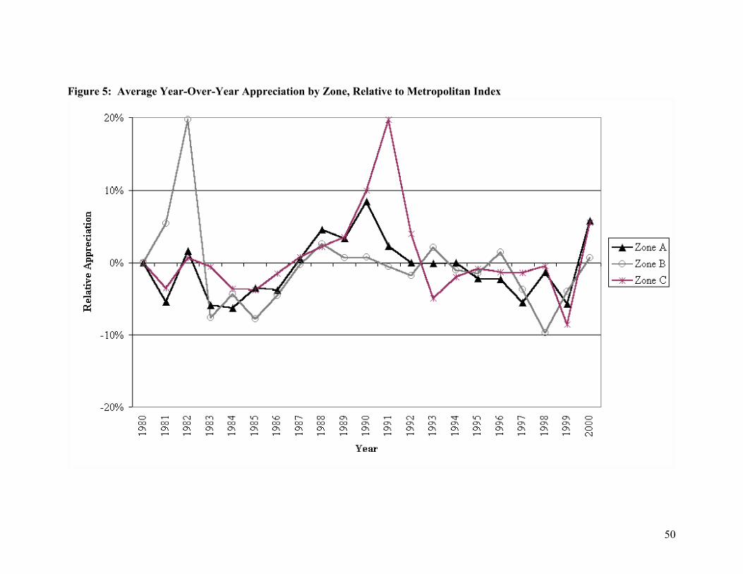
50

Figure 5: Average Year-Over-Year Appreciation by Zone, Relative to Metropolitan Index

51

Figure 6: Superstition Freeway Corridor and Metropolitan Phoenix Residential Price Appreciation Indexes

Note: Size-adjusted study area values were adjusted for estimated housing population in each zone, to reflect the difference in area for the larger control zone.

52

Figure 7: Average Year-Over-Year Appreciation in Superstition Freeway Corridor, Relative to Metropolitan Index

53

Sample Results for Condominiums and Townhomes Multiple-unit residential properties were evaluated using the same t-test and regression procedures as for detached single family homes. However, a smaller sample of recorded sales was collected for condominiums and townhomes in the study area, which led to greater variance in the test results. Several variables were also omitted from the multiple-unit residential analysis, as these were either not relevant or not recorded. For example, the minimal lot size (if any) and planned amenities of these developments generally precludes swimming pools for individual units – none were recorded in the property sample. Similarly, properties either had air conditioning in the vast majority of cases, or no cooling system in a few cases, so evaporative cooling was not considered for the analysis. Comparisons of the most influential variables are shown in the following section. As in the case of detached single-family residences, a t-test was used, when applicable, to determine whether observed differences in general characteristics were statistically significant. These general comparisons are then followed by zone-based and street-based regression analyses to determine the effects of location on multiple-unit housing prices. However, the smaller number of recorded sales made the regression analyses less reliable than those done for detached residential proeprty. Condominiums and Townhomes: Descriptive Statistics by Zone Statistically significant differences in structure and lot size were observed between multiple-unit residential properties in all zones. Structures in Zone A tended to be smallest, with an average size of 917 square feet. Zone B condominiums were largest, averaging 1,148 square feet. Zone C condos averaged 1,060 in size. Median structure size was virtually identical to average size for all zones, indicating that condos were normally distributed by structure size. Lot sizes shown in Table 11 were considerably more variable, with the largest average lot size (4,665 square feet) observed in Zone A. In contrast to Zone A lots, which ranged from 4,025 to 5,201 square feet, many properties in the remaining impact zone and the control zone did not have individual lots. A considerable amount of the variation in this sample may therefore be the result of combining several subclasses of multiple-unit residential properties. It is likely that the units with larger lot sizes were patio homes or row-house townhome developments. Properties with no lot space were likely flat-style condominiums with two or more units stacked vertically. For this analysis, it was assumed that all of these developments would still share enough characteristics (e.g. proximity to adjoining units, homeowner association and maintenance fees, larger percentage of renters) to warrant an aggregate comparison. However, the variety of development styles may have played a significant role in the relative value of properties in each zone.

54

Table 11: Summary of Structure and Lot Size for Condominiums by Zone

Structure Square Footage Lot Square Footage Measurement Zone A Zone B Zone C Zone A Zone B Zone C Mean 917 1,148 1,060 4,665 3,322 1,255 Median 906 1,169 1,052 4,602 2,971 0 Mode 823 1,237 792 4,600 2,949 0 Minimum 821 718 623 4,025 0 0 Maximum 1,056 1,476 1,619 5,201 6,059 9,945 Standard Deviation 93 218 207 277 1,311 2,073 Sig. Diff. from:1.

Zone A -- YES YES -- YES YES Zone B YES -- YES YES -- YES Zone C YES YES -- YES YES --

Notes: (1) Significant difference for 95% percent level of confidence indicated by p value less than 0.05 for t-test of mean values by zone.

Differences in structure age at the time of sale were not found to be statistically significant between zones. Average structure age ranged from 5.15 years in Zone B to 6.03 years in Zone C. Median age was 4 years in Zone A, 3 years in Zone B, and 5 years in Zone C. Condos in Zone B had the largest adjusted sales price on average, as shown in Table 12. Average and median adjusted sales prices were lowest in the control zone, $62,384 and $61,790 respectively. Properties in Zone A sold for an average of $65,759 in current dollars, and Zone B properties averaged $74,073. All of these differences were statistically significant at the 95 percent confidence level. Table 12: Summary of Structure Age and Price for Condominiums by Zone

Structure Age1. Adjusted Sale Price2. Measurement Zone A Zone B Zone C Zone A Zone B Zone C Mean 5.81 5.15 6.03 $65,759 $74,073 $62,384Median 4.00 3.00 5.00 $65,277 $74,013 $61,790Mode 0.00 0.00 0.00 n/a $83,008 $53,711Minimum 0.00 0.00 0.00 $44,205 $39,114 $28,651Maximum 15.00 17.00 25.00 $83,749 $105,578 $120,116Standard Deviation 5.75 5.10 5.56 $7,253 $13,335 $14,205Sig. Diff. from:3.

Zone A -- NO NO -- YES YES Zone B NO -- NO YES -- YES Zone C NO NO -- YES YES --

Notes: (1) Refers to age of structure in years at time of sale. (2) Actual sales price adjusted to constant dollars using the Phoenix-Mesa metropolitan housing price index (HPI). (3) Significant difference for 95% percent level of confidence indicated by p value less than 0.05 for t-test of mean values by zone.

55

Condominiums and Townhomes: Regression Analysis The regression model results for condominiums and townhomes were generally not as reliable as the results recorded for detached single family residences. This is likely a result of the smaller sample size for condos and townhomes. A total of 609 sales transactions were recorded for condos and townhomes. The data were more evenly distributed among the three zones, with 20.3 percent of sales in the abutting zone (A), 35.1 percent in impact zone B, and the remaining 44.6 percent in control zone C. The explanatory value of this model was between 64.6 percent for the zone-based analysis and 54.6 percent for the street-location analysis. Table 13: Condo and Townhome Regression Statistics

Zone-Based1. Street-Based2.

Multiple R 0.8039 0.7392 R Square 0.6463 0.5464 Standard Error 11,202 11,716 Observations 609 395 Notes: (1) Comparison of abutting zone A, impact zone B and control zone

C. (2) Comparison of Zone A with subsets of Zone C, based on street address on or off a major mile-street thoroughfare.

Regression results for condos and townhomes shown in the tables below had fewer variables than for detached single family residences. Insufficient quality data were available to distinguish between condominium structures, and none of the units tested had swimming pools or cooling systems other than air conditioning, so the pool and evaporative cooling variables were removed from the analysis. As in the case of detached single family residences, the coefficients for condominiums generally reflected the expected contribution of each housing component. However, the relative magnitude of each component tended to be quite different than in the detached single family analysis. Note that results for condos were not directly comparable to results for detached residences due to the differences in the number of variables considered in the analysis.16 In contrast with detached single-family residential property results, several variables were determined not to be statistically significant in the zone-based condo and townhome regression. P-values for number of bath fixtures, carport size, and the zone locations were all greater than 0.05, indicating that there was greater than a 5 percent likelihood that the coefficients for these variables were the product of random variation. However, the p-value for Zone B locations was only slightly greater than 0.05, so a less stringent confidence interval (e.g. 90 percent) would likely have produced statistically significant results.

16 The fewer variables considered, the greater the influence attributable to each variable. Therefore, the higher price per square foot for condos may simply reflect the omission of housing quality or other variables.

56

Also notable in the zone-based analysis are the positive values associated with each zone. Although these numbers were not statistically significant, the coefficients suggest that buyers of attached residential property had different priorities in terms of housing amenities. However, at the level of confidence chosen, no conclusion could be reached regarding the value of location in the zone-based analysis.

Table 14: Zone-Based Regression Coefficients for Condominiums and Townhomes

Confidence Interval Variable Coefficient Standard Error t-Stat P-value

Lower 95% Upper 95%Intercept 0 #N/A #N/A #N/A #N/A #N/A Bldg. Sq. Ft. $65.95 $3.63 18.1681 0.00000000 $58.82 $73.08Lot Sq. Ft. $1.41 $0.32 4.42767 0.00001132 $0.78 $2.04Bath Fxtrs. $581.19 $553.90 1.04928 0.29447366 -$506.62 $1,669.01Age -$836.53 $86.82 -9.6355 0.00000000 -$1,007.03 -$666.02Porch/Patio $8,217.61 $1,096.91 7.49161 0.00000000 $6,063.36 $10,371.87Air Cond. $7,899.88 $1,957.61 4.03548 0.00006155 $4,055.27 $11,744.48Carport $1,492.57 $1,482.60 1.00672 0.31447353 -$1,419.15 $4,404.29Garage $7,106.48 $1,254.13 5.66645 0.00000002 $4,643.45 $9,569.51Zone A $2,705.99 $1,735.05 1.5596 0.11938316 -$701.54 $6,113.51Zone B $2,780.06 $1,441.49 1.92861 0.05425182 -$50.92 $5,611.04

Regression results comparing the Zone A properties to control area (Zone C) locations on and off major surface streets indicated that higher condominium property values were associated with major thoroughfares. Although the street-based analysis shown in Table 15 had a lower explanatory value overall, statistically significant results were reached for a greater number of variables. In the street-location analysis, only bath fixtures had a p-value that was not significant at the 95 percent level of confidence. Most variables that were statistically significant in both regressions (e.g. structure and lot size, age), fell within the confidence intervals predicted by the other model. However, the smaller sample size and slightly larger p-values for most variables in the street-location analysis made the confidence intervals for estimated values of each housing characteristic quite large. Nonetheless, the street-location analysis resulted in statistically significant coefficients at the 95 percent level of confidence for differences in location. The street-based regression results indicated that access was a positive amenity for buyers of attached residential units. Condo and townhome sales both in Zone A and on primary streets in Zone C were valued at a premium to control zone properties located on smaller thoroughfares, all other characteristics being equal. A slightly higher premium was placed on locations adjacent to the freeway than on locations located on major (mile) streets, as indicted by the coefficients for these variables. In year 2000 housing price dollars, the estimated premium was $5,162 for Zone A locations and $4,654 for primary-

57

street locations, relative to the control properties. The 95 percent confidence interval for the Zone A location premium ranged from $358 to $9,966 (in year 2000 dollars), while the primary street locations had a premium ranging from $1,679 to $7,629 at the same level of confidence.

Table 15: Street-Based Regression Coefficients for Condominiums and Townhomes

Confidence Interval Variable Coefficient Standard Error t-Stat P-value

Lower 95% Upper 95%Intercept 0 #N/A #N/A #N/A #N/A #N/A Bldg. Sq. Ft. $63.37 $4.69 13.5085 0.00000000 $54.14 $72.59Lot Sq. Ft. $1.31 $0.40 3.2777 0.00114169 $0.52 $2.10Bath Fxtrs. $379.87 $738.82 0.51416 0.60743400 -$1,072.75 $1,832.49Age -$917.34 $110.40 -8.3095 0.00000000 -$1,134.39 -$700.28Porch/Patio $5,836.08 $1,799.57 3.24304 0.00128580 $2,297.87 $9,374.29Air Cond. $6,959.82 $2,757.72 2.52376 0.01201212 $1,537.75 $12,381.89Carport $4,649.24 $2,015.00 2.30732 0.02156671 $687.47 $8,611.02Garage $12,248.78 $2,045.57 5.98795 0.00000000 $8,226.89 $16,270.67Zone A $5,161.74 $2,443.36 2.11255 0.03528220 $357.73 $9,965.74Major Street $4,653.80 $1,513.15 3.07557 0.00225099 $1,678.73 $7,628.87

Whereas the price differences observed in the zone-based analysis may have been primarily the result of lot size and housing style discussed in the previous section, the primary street location analysis for condominiums and townhomes suggested that buyers of these properties place a greater emphasis on immediate access to a major thoroughfare. However, several points bear noting. The nature of these types of developments is such that an individual unit may be sheltered from the impacts of traffic and still have an address location on the through street. More so than with detached residential units, condominiums and townhomes benefit from community landscaping, perimeter walls and the close proximity of other units as a potential buffer from traffic-induced noise and other effects. Therefore, some degree of caution should be used in assessing these results. Because the analysis did not distinguish between individual units in a complex based on actual distance from the thoroughfare, it is possible that some units actually experienced some differential in pricing based on this distance. The relatively low explanatory value of this analysis suggests that better means of distinguishing between units would have yielded superior results. Nonetheless, the overall picture indicates that major streets, including freeways, present a more desirable location for the development of multiple-unit communities. This may reflect some difference in consumer preference for locational amenities between buyers of detached and attached residential properties.

58

Vacant Land Value Results for Residential Parcels Land sales are inherently difficult to compare, in that ordinary methods of standardizing value (e.g. price per square foot) are not linearly related (Palmquist, 1980). All other things being equal, price per square foot tends to rise as parcel size shrinks.17 This creates a problem when comparing parcels of substantially different sizes. For example, the price per square foot calculation may yield substantially different results for a 5,000 square foot parcel and a 20,000 square foot parcel, even if the two parcels have similar site characteristics in all other aspects. A comparison of these two parcels based on price per square foot would thus lead one to erroneously conclude that the smaller parcel was more valuable. This research attempted to control for price per square foot variance in vacant parcels by fitting a logarithmic equation with recorded sales of vacant residential land in each zone. The results of this calculation are shown in Figure 8. Note that while the “fit” appears to be nearly perfect, there were very few data points from which to plot the equation. Therefore, the equation was assumed not to be statistically significant, and was used only as the basis for a rough estimation of land values. This equation was then used to predict the expected value for each parcel, which was subsequently compared to the actual sales value for each vacant parcel. The results of the comparison are shown in Table 16 on the following page. Figure 8: Time-Adjusted Sales Value for Vacant Residential Land by Lot Size

17 Note that this is also true of structure size, but the relatively limited variability in structure size tends to mitigate this effect for all but the most extreme cases.

59

Although parcels in Zone A were smallest, and thus commanded the highest sales price per square foot, the predicted value for Zone A parcels exceeded the actual sales value. When compared with Zone B and Zone C, the parcels in Zone A sold for less than would be expected based on size. While not statistically significant, this finding suggests that residential land immediately adjacent to the freeway is discounted in the same way as developed structures. However, it is also entirely possible that other site characteristics were responsible for the lower sale values in Zone A. Table 16: Comparison of Vacant Residential Land Values by Zone

Diff. In Adj. Sale Price2. Diff. Per Sq. Ft.3.

Zone Sale Records

Avg. Price / Sq, Ft.1.

Avg. Lot Size Average Median Average Median

A 3 $4.60 4,032 -$2,147.91 -$1,843.06 -$0.50 -$0.41 B 8 $2.10 56,420 $4,131.84 $6,341.80 $0.26 $0.26 C 6 $3.58 10,519 -$3,041.15 -$786.98 $0.01 -$0.03 C 4. 3 $5.26 4,637 $1,575.79 $1,230.50 $0.36 $0.25 All 17 $3.06 27,337 $492.01 -$1,182.90 $0.04 -$0.07

Notes: (1) All prices adjusted for year of sale using metro Phoenx HPI. (2) Based on actual sale price in constant dollars less the expected sale price derived from function shown in Figure 8. (3) Actual versus expected sale price per square foot. (4) Zone C results for lots under 6,000 square feet.

Comparisons can also be made based on the average price per square foot for an entire area. In this case, the influence of the most extreme parcel sizes will be somewhat reduced by other parcels in the area. Note however, that just as new construction may influence the distribution of housing prices per square foot (see “Previous Impact Analysis of the Superstition Freeway” above), so might subdividing parcels significantly increase the mean price of land per square foot in the area. Several of the parcels in Zone B included in Table 16 were not subdivided, which is generally associated with much larger parcel sizes and lower price per square foot. In cases where sufficient data exist, this effect might be controlled through sample selection. However, the limited number of parcels available for this analysis precluded sample restrictions. In order to estimate comparative residential land values in a more comprehensive manner, an index of average land values was created using the assessed land value per square foot for developed parcels. It was assumed that the characteristics of parcels that had already been developed would be more similar than undeveloped parcels of various sizes, thereby reducing the variation in value per square foot. Although the county assessor’s records break out land value from total assessed valuation, it was recognized that assessed values may vary substantially from the sales price that a property might command in the market. The indexed values shown in Figure 9 below might thus be considered as representative of perceived value, which may or may not be correlated with actual value. Viewed in this manner, it appears that a persistent gap exists between perceived land values in Zone A and the control area, with the former discounted in assessed value relative to the latter. However, land value estimates for Zone B did not appear to be subject to the same discounting, though this may be due to the statistically significant difference in lot size for Zone B (see Table 4).

60

Figure 9: Average Assessed Value per Square Foot, Residential Land

Note: Land values based on Maricopa County Assessor records, and may not be current at the time a sale was recorded.

61

Sample Results for Commercial and Industrial Properties Commercial property data available were severely limited. Most property sales had not been dated, and characteristics such as structure and lot size were only recorded for a small subset of the available locations. In addition, most commercial locations were not recorded with an address from which zones could be assigned. These limitations make the following assessment of commercial property sales tenuous at best. When available, data have been presented in as informative a manner as possible, but in no case should be considered statistically significant. A total of eight vacant commercial land parcels were identified for the land value analysis. The commercial land sales data were incomplete, with sales prices not available for three of the eight parcels and sales dates missing from all property records. The land value assessment was therefore made using assessed land values from Maricopa County records. As in the case of vacant residential properties, a logarithmic function was used to predict expected values for vacant commercial land. Again, the limited number of data points make the equation unstable, and useful only as a rough predictor. This equation is shown in Figure 10. Figure 10: Assessed Value for Vacant Commercial Land by Lot Size

Predicted land value was compared to assessed land value to estimate whether parcels were being perceived as more or less valuable depending on location.18 The results shown in Table 17 suggest that vacant commercial land in Zone B, closer to the 18 Assessed valuation was assumed to be a reliable indicator of perceived value, but not necessarily market value. This distinction is made because an assessor is not a “transaction party” interested in buying or selling the parcel being assessed. Thus while the assessment may be an objective analysis, it may not reflect market value for the property.

62

Superstition Freeway, was perceived to be more valuable than would be expected based on results for the control zone. Control zone parcels averaged a slightly higher assessed value relative to expected value, but not to the extent shown for the parcel in Zone B. Once again, other site characteristics may have influenced the perceived value of the Zone B parcel, and given the limited sample size, this disparity could not be directly attributed to the Superstition Freeway. Table 17: Vacant Commercial Land Values (Assessed)

Total Difference2. Difference per Sq. Ft.3.

Zone Parcels Avg. Val. /

Sq, Ft.1. Avg. Lot

Size Average Median Average Median B 1 $4.00 39,988 $14,103 $14,103 $0.35 $0.35 C 7 $3.85 39,944 $3,222 -$6,368 $0.12 -$0.15

All 8 $3.86 39,950 $4,582 -$2,401 $0.15 -$0.10 Notes: (1) Assessed value per square foot from Maricopa County Assessor records. (2) Difference in

actual versus expected assessed land values based on explanatory function shown in Figure 10. Note that assessed land value is not necessarily an accurate indicator of true value. (3) Actual versus expected assessed value per square foot.

Although the commercial land value analysis was inconclusive, the distribution of commercial development in Mesa suggests that a premium is placed on locations closer to the freeway. The shaded areas in Figure 11 show concentrations of commercial development along several corridors. Strip developments appear to be heaviest along Main Street, but the largest concentrations are clearly shown along US60 at Alma School and Power Roads – sites of Fiesta Mall and Superstition Springs Mall respectively. Several researchers have noted that these regional malls were the primary drivers of commercial growth in the Superstition Freeway corridor (Tomasik, 1987; Newell, 1991). In contrast with commercial development, industrial development appears to be less influenced by immediate proximity to the freeway. Mesa industrial sites locations shown in Figure 12 are most heavily concentrated around the two local airports, with smaller clusters along Main Street, Broadway, and the Superstition Freeway. Although the Superstition Freeway does not appear to have such an immediate influence on industrial development, it is worth noting that the industrial sites are clustered around transportation nodes. In addition to the airport developments, the Main Street and Broadway locations are proximate to the Pima Freeway (SR101). Thus it appears that access to transportation facilities does play a role in industrial development, but that the benefits associated with locational access are dispersed across a wider area than for commercial locations.19 Also evident in the dispersal diagrams is the likelihood that a specific mode (i.e. automobile transportation) is most highly correlated with consumer and commuter-driven development, whereas industrial sites appear to be chosen based on the most advantageous mode for the industry. 19 It may also be the case that zoning decisions were the primary driver of development. However, Tomasik notes that, in contrast to planned development in Tempe, development in Mesa was primarily driven by the market (Tomasik, 1987). This indicates that commercial and industrial location decisions in Mesa were made with more regard for site advantages that might accrue to property owners at a location.

63

Figure 11: Commercial Development in the US60 Corridor

Source: Planning Department, City of Mesa, 1999. Figure 12: Industrial Development in the US60 Corridor

Source: Planning Department, City of Mesa, 1999.

64

Separate analyses of nonresidential property sales were done for six major property types. Sales were only recorded in Zone B and Zone C, permitting only general statements about the influence of location. Because property data were generally limited to type, structure size and lot size, the analysis was focused on sale value attributable to land and improvements. The sales price was allocated between buildings (if any) and land based on the ratio of assessed land value to total assessed value, with the difference allocated to structures. Each sale value was then converted to a price per square foot for both structure and land. These results should be viewed with caution, as sale dates were not available in the database. It is virtually certain that property values fluctuated significantly over the twenty-year period, so these results provide only an overview of average prices for the entire period. Sales results for office and financial buildings are shown in Table 18. A total of three sales were recorded in the impact zone B, and 20 sales in control zone C. The structures were of similar size, but sold for a wide range of prices per square foot of space. The median values for Zone B and Zone C were similar, but average sales prices were influenced by a large relative sales price for one transaction in Zone B. Lot size was not recorded for transactions in Zone B. Office properties in Zone B were somewhat newer than those in Zone C. The average year built in Zone B was 1987 versus 1985 for Zone C. Both zones had a median year of construction of 1986. Table 18: Summary of Office Property Characteristics by Zone

Average Median Office Properties Zone B Zone C All Zone B Zone C All

Structure Sq.Ft. 5,424 6,619 6,463 5,256 4,704 5,002 Land Sq.Ft. n/a 46,298 46,298 n/a 45,563 45,563 Structure Price/Sq.Ft.1. $75.09 $54.66 $57.32 $52.96 $55.92 $52.96Land Price/Sq.Ft.2. n/a $1.52 $1.52 n/a $1.48 $1.48Notes: (1) Prices were not adjusted for date of sale. Structure sales price estimated based on ratio of net

structure assessed value (i.e. less land value) to total assessed value. (2) Land sales price estimated based on ratio of land value to total assessed value.

The largest number of sales transactions were recorded for retail properties (Table 19). Not surprisingly, this group also exhibited the most convergence in land prices per square foot. However, the lot sizes were substantially larger in Zone C, suggesting that the apparent land price differential for Zone B would not exist if the parcels were of similar size. Structures were of comparable size in both zones, with slightly larger buildings in Zone B. Samples for both zones were split between single stores and community shopping centers. As in the case of office properties, Zone B retail structures tended to be newer – built in 1987 on average versus 1985 for Zone C. While this may partially explain the difference in price per square foot for retail structures, it is more likely that the date of sale and unrecorded property characteristics had the greatest influence. Nonetheless, the structure sale value per square foot was substantially higher in Zone B, on both an average and a median basis.

65

Table 19: Summary of Retail Property Characteristics by Zone

Average Median Retail Properties Zone B Zone C All Zone B Zone C All

Structure Sq.Ft. 27,084 24,346 24,812 11,830 11,700 11,700 Land Sq.Ft. 39,988 106,393 103,230 39,988 60,309 56,802 Structure Price/Sq.Ft.1. $110.67 $69.14 $76.21 $98.58 $49.80 $54.59Land Price/Sq.Ft.2. $3.78 $3.63 $3.64 $3.78 $2.73 $2.80Notes: (1) Prices were not adjusted for date of sale. Structure sales price estimated based on ratio of net

structure assessed value (i.e. less land value) to total assessed value. (2) Land sales price estimated based on ratio of land value to total assessed value.

A total of seven sales transactions were recorded for the restaurant category in Zone B and six transactions in Zone C. Lot size data were not available for any of the recorded transactions. As indicated in Table 20, both average and median restaurant structure size tended to be similar between zones. Although substantial variation was evident in the average structure values per square foot, the median values were quite similar. Average and median year of construction in Zone B were both 1986. While the average year of construction in Zone C was 1985, the median was 1987. The convergence of these values suggests that the restaurant results were more reliable for structure price than previous property types. However, restaurant properties included several classes of food establishment (e.g. sit-down restaurants, bars, and fast-food restaurants), and it was not known whether a significant difference in standardized sale price normally exists between properties of these various types. Table 20: Summary of Restaurant Property Characteristics by Zone

Average Median Restaurant Properties Zone B Zone C All Zone B Zone C All

Structure Sq.Ft. 2,950 3,422 3,212 2,919 2,946 2,946 Land Sq.Ft. n/a n/a n/a n/a n/a n/a Structure Price/Sq.Ft.1. $183.74 $295.29 $245.71 $202.67 $205.98 $205.98Land Price/Sq.Ft.2. n/a n/a n/a n/a n/a n/aNotes: (1) Prices were not adjusted for date of sale. Structure sales price estimated based on ratio of net

structure assessed value (i.e. less land value) to total assessed value. (2) Land sales price estimated based on ratio of land value to total assessed value.

The largest difference in commercial structure age was observed for apartment communities.20 Apartment buildings in Zone B were built in 1986 on average, versus 1982 for Zone C apartments. As indicated in Table 21, the Zone B apartment buildings tended to be larger as well, with an average structure size of 219,228 square feet and a median size of 218,881 square feet. Zone C apartment communities had an average 20 Apartment communities have been grouped with other “nonresidential” properties because the purchase decision for an apartment building is virtually always a commercial decision. Whereas most detached homes and many condominiums are sold to owner-occupants, apartment communities are sold based on expected income from rental transactions and were thus considered “commercial” for this analysis.

66

structure size of 189,629 square feet and a median size of 185,636 square feet. A total of four apartment building sales were recorded in Zone B, and 16 sales were recorded in Zone C. Average and median prices per square foot for apartments were larger in Zone B on all measures. Structure and land prices per square foot were larger than in Zone C despite the larger size of Zone B buildings and lots. As shown in the land value analysis equations, this is the opposite effect that would be expected. While it can not be concluded from the data available that an accessibility premium is attached to apartment developments closer to the Superstition Freeway, these results do appear to follow the same trend as observed for other multifamily developments (i.e. condominium and townhome sales). Table 21: Summary of Apartment Property Characteristics by Zone

Average Median Apartment Properties Zone B Zone C All Zone B Zone C All

Structure Sq.Ft. 219,228 189,629 199,495 218,881 185,636 191,883 Land Sq.Ft. 504,217 391,735 429,229 492,968 412,622 492,968 Structure Price/Sq.Ft.1. $59.28 $38.89 $42.97 $38.13 $33.39 $33.56Land Price/Sq.Ft.2. $3.92 $1.25 $2.14 $2.57 $1.32 $1.61Notes: (1) Prices were not adjusted for date of sale. Structure sales price estimated based on ratio of net

structure assessed value (i.e. less land value) to total assessed value. (2) Land sales price estimated based on ratio of land value to total assessed value.

The sample of industrial properties consisted of a single sales transaction for each zone. Given the variance in industrial structure and lot size, shown in Table 22, no relationships in the data could be identified. It appears that properties shown in Table 22 are for different types of industrial uses. The relatively large lot size in Zone B suggested a more land-intensive operation such as an automotive repair or storage lot, whereas the Zone C property was likely a more capital intensive operation (e.g. small-scale manufacturing). The differences in usage and size likely had the most influence on pricing disparities, and the limited sample permitted no hypotheses regarding location. Table 22: Summary of Industrial Property Characteristics by Zone

Average Median Industrial Properties Zone B Zone C All Zone B Zone C All

Structure Sq.Ft. 1,500 4,356 2,928 1,500 4,356 2,928Land Sq.Ft. 203,773 15,246 109,510 203,773 15,246 109,510 Structure Price/Sq.Ft.1. $61.14 $33.95 $47.55 $61.14 $33.95 $47.55Land Price/Sq.Ft.2. $0.41 $3.42 $1.91 $0.41 $3.42 $1.91Notes: (1) Prices were not adjusted for date of sale. Structure sales price estimated based on ratio of net

structure assessed value (i.e. less land value) to total assessed value. (2) Land sales price estimated based on ratio of land value to total assessed value.

67

Agricultural property sales were evaluated solely on the basis of land prices. In this case, a significant discrepancy was noted between median and average values in Zone C, despite 15 recorded sales in the area. On an average basis, property prices per square foot were higher in Zone C than for the single sale recorded in Zone B. However, these were significantly influenced by several large transactions, as indicated by the lower median sale price. In addition to the variation expected from changes in date of sale, it was not clear whether land classified as agricultural was actually sold for agricultural use. Given the development history in the Superstition Freeway corridor, it may be that agricultural land was sold to residential developers for new subdivisions. Such use would generally be associated with higher relative land values. Table 23: Summary of Agricultural Property Characteristics by Zone

Average Median Agricultural Properties Zone B Zone C All Zone B Zone C All

Structure Sq.Ft. n/a n/a n/a n/a n/a n/a Land Sq.Ft. 499,676 536,029 533,000 499,676 420,441 428,021 Structure Price/Sq.Ft.1. n/a n/a n/a n/a n/a n/aLand Price/Sq.Ft.2. $1.80 $2.66 $2.59 $1.80 $0.19 $0.22Notes: (1) Prices were not adjusted for date of sale. Structure sales price estimated based on ratio of net

structure assessed value (i.e. less land value) to total assessed value. (2) Land sales price estimated based on ratio of land value to total assessed value.

Nonresidential Summary Although the analysis was limited by the availability of nonresidential sales data and transaction details, a few tentative assessments may be made from the information on hand. First, the Superstition Freeway appeared to exert a greater influence on the development of commercial property sites than industrial property sites in Mesa. This is likely due to the greater reliance of many commercial establishments on a single transportation mode (i.e. automobiles). The observed values per square foot for vacant commercial land suggest that demand for commercial space was slightly greater in the impact zone (B) than in areas further from the freeway (Zone C). Results for office and retail properties also appear to support this observation. However, results for restaurant properties showed a bias toward higher values in Zone C, which would not be expected if the freeway afforded some locational advantage. Apartment buildings tended to have higher sale values in Zone B, which corroborated findings for condominiums. It appears that buyers of attached residential property place a greater emphasis on access to surrounding facilities than do buyers of detached residential property. This observation rests on the assumption that the value of apartment communities is based on the expected rental income from tenants, which would reflect tenants willingness to pay for the amenities associated with the apartment community. Note that despite the observation of these weak trends, none of these cases can be considered conclusive.

68

V. Conclusions Freeway development confers benefits to highway users in the form of reduced transportation costs. This reduction in transportation costs can have a variety of spill over effects on highway users and nonusers alike. Previous research has identified a number of population, economic and land use effects that tend to accompany freeway development. By improving the access to locations along the freeway corridor, construction makes these sites more attractive to development. People are more willing to live farther from major employment centers if they have a faster way to get to work. Industries are more likely to consider locations further from commercial districts if they can be certain of good accessibility for their workers and their goods and supplies (Buffington, et al, 1985). The effect of these changes in access are usually observed in an increase in population and commercial activity in the freeway corridor (Gamble, 1978). As individuals and firms relocate to areas serviced by the new freeway, economic activity tends to rise in the corridor. This increased demand for homes and commercial land has generally been associated with an increase in property values in the transportation corridor, as savings from reduced transportation costs are capitalized into asset values (Forkenbrock, 1990). However, most researchers caution that gains in one area are frequently losses in another, and a broader impact assessment should evaluate the changes brought about by migration of firms and individuals from other areas. Freeway development can also impose costs on users and nonusers. Highway users may suffer in the short term as construction diverts traffic onto smaller local streets. All drivers share the added costs of congestion in the form of lost time and higher vehicle operating costs (Rowell, et al, 1997). Property owners may also suffer, both in the short term as construction reduces access to local homes and businesses, and in the longer term as added traffic noise and pollution adversely impact properties closest to the highway. Considered in conjunction with the benefits that accrue to property owners due to freeway development, these negative impacts have generally been interpreted as evidence that freeways impose costs on certain property owners that may or may not be offset by gains. A substantial body of research has been devoted to the examination of this “distribution effect,” in which the benefits and costs of freeway development are not distributed equally among property owners. Most research has focused on changes in single-family residential properties, probably for two reasons. First, data on residential property sales are easily gathered, and housing characteristics more comparable than many commercial properties (e.g. the differences between classes of office space). Second, residential property owners tend to be the most vocal opponents of freeway development, as commercial property owners generally welcome the benefits of proximity to a freeway (Lewis, et al, 1997).

69

Freeway construction has been shown to stimulate migration to freeway corridors (Gamble, 1978) and to increase the amount of residential and commercial development in the corridor (Buffington, et al, 1985), but may lead to a decline in marketability for existing residential units (Burkhardt, 1984). Previous research has identified a persistent negative impact on homes located closest to freeways, though in many cases these effects are small (Langley, 1981; Allen, 1981) or more than offset by net gains in the surrounding area due to increased accessibility (Palmquist, 1980). This research identified similar results for residential properties located in the Superstition Freeway corridor. However, additional analysis of different types of residential property and the general influence of all traffic yielded new insights. Among the findings were the following: �� Detached single-family homes were adversely impacted by proximity to the freeway.

The negative effects on sale prices were greatest for homes adjacent to the freeway, but a reduction in property values was also observed in the impact area (within ½ mile of US60).

�� Price appreciation was also lower for single-family homes nearest the freeway, indicating that negative impacts were not transitory, but lasting.

�� Overall price appreciation in the Superstition Freeway corridor suggested that the negative impacts to some property owners were more than offset by housing price appreciation in the surrounding areas. Average sales price appreciation for Mesa and Gilbert single-family homes within 5 miles of the freeway (including adversely affected properties) was higher than housing price appreciation in the metropolitan area.

�� The negative impact on single-family housing values associated with proximity to the freeway was also found to exist for homes located on major surface streets. An inverse correlation between freeway traffic levels and housing prices was observed as well.

�� Multiple-unit residential developments appeared to benefit from proximity to the freeway, and from locations on major surface streets, suggesting that owners of these types of properties had different preferences in terms of locational amenities than owners of detached single-family homes. Condominium owners were found to experience a slight rise in property values when the property was located in the zone adjacent to the Superstition Freeway or on a major mile street.

The data available permitted only a cursory comparison of commercial and other nonresidential properties in the Superstition Freeway corridor. Vacant commercial land appeared to be valued more highly than expected. While comparable property values were observed for restaurants and office properties in the impact and control areas, retail properties appeared to command higher prices closer to the freeway. A pricing differential was also observed for large apartment buildings, which were priced at a premium to apartments in the control zone, reinforcing the results obtained for condominiums and townhomes.

70

Perhaps the most important finding of this research is the correlation between traffic and residential property values. Although researchers have traditionally focused on freeway corridors to evaluate property value effects, the implicit assumption is that proximity to traffic is at the root of any negative impacts on residential properties. Viewed in this context, the freeway itself is nothing more than a conduit for traffic effects. The same negative effects were observed for single-family homes located on major mile streets more than ½ mile from the Superstition Freeway. Motor vehicle traffic on a particular route is a complex derivation from a number of related influences, including local population, automobile ownership, driver preferences, the number and characteristics of alternate routes and/or modes of transportation, and the amount of commercial activity in an area. Clearly, freeway development can have an influence on some of these variables. If there is traffic generated by the freeway, the net impact of traffic in general will be greater (Hibbard, et al, 1974). If sufficient alternate routes exist, property owners may experience smaller accessibility benefits from freeway construction (Palmquist, 1980). However, freeways tend to concentrate traffic in a more localized area. If a region experiences growth in traffic without the benefit of freeway development, traffic will be dispersed over a wider area. Although this may have less of an impact on a specific group of property owners, it is probable that more properties will be exposed to the negative effects of traffic. Freeway development is a trade-off between accessibility and traffic growth. But the same can be said for construction of any roadway. The effects of traffic form the basis for changes in property values – whether positive, as might be expected for commercial establishments servicing a mobile population, or negative, as expected from residential proximity to traffic noise and air pollution. Whether a thoroughfare is classified as a highway or a local street may not be as important as the volume of traffic carried. Assessments of the net effects of freeways on nearby property values are limited in that opposition to freeway development is typically the impetus for further research. However, in recognizing that the freeway is simply another means of carrying traffic, the analysis shifts to the benefits and costs of the road system in general; in other words, the impact of traffic. It is recommended that further research examine the incremental changes in property values with respect to differences in traffic volumes, in order to clarify the relationship between these variables.

71

References Allen, Gary. Highway Noise, Noise Mitigation, and Residential Property Values. In Transportation Research Record 812: Economic, Social, and Energy Effects of Highway Transportation. TRB, Washington, DC, 1981.

Arizona Department of Transportation. “Superstition Freeway Overview.” 2000.

Buffington, Jesse, Margaret Chui and Jeffery Memmott. Effects of Freeway Stage Construction on Nearby Land Uses and Vehicle User Costs. In Transportation Research Record 1046: Economic Development, Land Use Modeling, and Transportation Requirements. TRB, Washington, DC, 1985.

Burdick, Richard. Instructional Materials for Quantitative Business Analysis. Department of Business Administration, Arizona State University, 1998.

Burkhardt, John. Socioeconomic Reactions to Highway Development. In Transportation Research Record 991: Social and Technological Issues in Transportation Planning. TRB, Washington, DC, 1984.

Forkenbrock, David. Putting Transportation and Economic Development into Perspective. In Transportation Research Record 1274: Transportation and Economic Development, 1990. Transportation Research Board, National Research Council. Washington, DC, 1990.

Gamble, Hays B. and Thomas B. Davinroy. NCHRP Report 193: Beneficial Effects Associated With Freeway Construction, Environmental, Social and Economic. Transportation Research Board, National Research Council, Washington, DC, 1978.

Gillespie, James. I-73 Economic Impact Analysis. Virginia Transportation Research Council, Charlottesville, VA. January, 1995.

Hagler Bailly Services, Inc. and Morpace International, Inc. NCHRP Report 436: Guidance for Communicating the Economic Impacts of Transportation Investments. Transportation Research Board, National Research Council, Washington, Dc, 1999.

Hibbard, Thomas and Fred Miller. Economic Analysis and the Environmental Overview: Suggestions for Project Recommendations by Local Governments. In Transportation Research Record 490: Cost-Benefit and Other Economic Analyses of Transportation. TRB, Washington DC, 1974.

Johnson and Zaddack, Inc. Historical Property Sales Data – Metropolitan Phoenix. www.powermaps.com, 2000.

Kuzma JW. Basic Statistics for the Health Sciences, 3rd Edition. Mayfield Publishing Company, 1998.

72

Langley, C. John, Jr. Highways and Property Values: The Washington Beltway Revisited. In Transportation Research Record 812: Economic, Social, and Energy Effects of Highway Transportation. TRB, Washington, DC, 1981.

Lewis, Carol, Jesse Buffington, Sharada Vadali, and Ronald Goodwin. Land Value and Land Use Effects of Elevated, Depressed, and At-Grade Level Freeways in Texas. Texas Transportation Institute, Texas Department of Transportation. July, 1997.

Mahady, Francis and Dianne Tsitsos. Economic Impact of I-78 in Allentown, Pennsylvania. In Transportation Research Record 812: Economic, Social, and Energy Effects of Highway Transportation. TRB, Washington, DC, 1981.

Morris, Brent. Factors Affecting Land Values Near Proposed Beltway Exits. Department of Geography and Earth Sciences, University of North Carolina, Charlotte. December, 1998.

Newell, Kevin. The Impact of Freeways. Burns International. December, 1991.

Palmquist, Raymond. Impact of Highway Improvements on Property Values in Washington. Washington State Transportation Commission, Transportation and Planning Division, Washington State Department of Transportation. March, 1980.

Perera, Max. Framework for Classifying and Evaluating Economic Impacts Caused by a Transportation Improvement. In Transportation Research Record 1274: Transportation and Economic Development, 1990. Transportation Research Board, National Research Council. Washington, DC, 1990.

Rowell, Matt, Frederic Buonincontri, and John Semmens. The Cost Effectiveness and Magnitude of Potential Impact of Various Congestion Management Measures. Transportation Research Center, Arizona Department of Transportation, 1997.

Sherwood, Robbie. The Going Gets Tougher on US60. In Arizona Republic. June 22, 2001.

Simple Interactive Statistical Analysis (SISA). SISA Online, 2000.

Spawn, David and David Hartgen. Urban Loops, Access, and the Cost of Land: A Preliminary Study. Center for Interdisciplinary Transportation Studies, University of North Carolina, Charlotte. May, 1997.

Tomasik, Jack. Socioeconomic and Land Value Impact of Urban Freeways in Arizona. Arizona Department of Transportation. October, 1987.

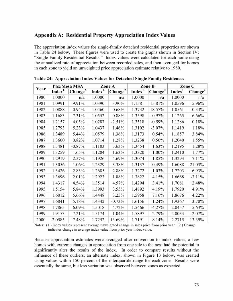
73

Appendix A: Residential Property Appreciation Index Values The appreciation index values for single-family detached residential properties are shown in Table 24 below. These figures were used to create the graphs shown in Section IV: “Single Family Residential Results.” Index values were calculated for each home using the annualized rate of appreciation between recorded sales, and then averaged for homes in each zone to yield an unweighted price appreciation estimate relative to 1980. Table 24: Appreciation Index Values for Detached Single Family Residences

Phx/Mesa MSA Zone A Zone B Zone C Year Index1. Change2. Index1. Change2. Index1. Change2. Index1. Change2.

1980 1.0000 n/a 1.0000 n/a 1.0000 n/a 1.0000 n/a 1981 1.0991 9.91% 1.0390 3.90% 1.1581 15.81% 1.0596 5.96% 1982 1.0888 -0.94% 1.0460 0.68% 1.3732 18.57% 1.0561 -0.33% 1983 1.1683 7.31% 1.0552 0.88% 1.3598 -0.97% 1.1265 6.66% 1984 1.2157 4.05% 1.0287 -2.51% 1.3518 -0.59% 1.1286 0.18% 1985 1.2793 5.23% 1.0437 1.46% 1.3102 -3.07% 1.1419 1.18% 1986 1.3489 5.44% 1.0579 1.36% 1.3173 0.54% 1.1857 3.84% 1987 1.3600 0.82% 1.0714 1.28% 1.3238 0.50% 1.2040 1.55% 1988 1.3481 -0.87% 1.1103 3.63% 1.3454 1.63% 1.2195 1.28% 1989 1.3259 -1.65% 1.1284 1.63% 1.3320 -1.00% 1.2410 1.77% 1990 1.2919 -2.57% 1.1926 5.69% 1.3074 -1.85% 1.3293 7.11% 1991 1.3056 1.06% 1.2329 3.38% 1.3137 0.49% 1.6088 21.03% 1992 1.3426 2.83% 1.2685 2.88% 1.3272 1.03% 1.7203 6.93% 1993 1.3696 2.01% 1.2923 1.88% 1.3822 4.15% 1.6668 -3.11% 1994 1.4317 4.54% 1.3514 4.57% 1.4294 3.41% 1.7081 2.48% 1995 1.5154 5.84% 1.3993 3.55% 1.4892 4.19% 1.7920 4.91% 1996 1.6012 5.66% 1.4448 3.25% 1.5958 7.16% 1.8676 4.22% 1997 1.6841 5.18% 1.4342 -0.73% 1.6156 1.24% 1.9367 3.70% 1998 1.7865 6.09% 1.5018 4.72% 1.5466 -4.27% 2.0457 5.63% 1999 1.9153 7.21% 1.5174 1.04% 1.5897 2.79% 2.0033 -2.07% 2000 2.0585 7.48% 1.7252 13.69% 1.7191 8.14% 2.2715 13.39%

Notes: (1.) Index values represent average unweighted change in sales price from prior year. (2.) Change indicates change in average index value from prior year index value.

Because appreciation estimates were averaged after conversion to index values, a few homes with extreme changes in appreciation from one sale to the next had the potential to significantly alter the results of the index. In order to compare results without the influence of these outliers, an alternate index, shown in Figure 13 below, was created using values within 150 percent of the interquartile range for each zone. Results were essentially the same, but less variation was observed between zones as expected.

74

Figure 13: Single Family Residential Appreciation Index for Interquartile Range by Zone

Note: These results are not directly comparable to metropolitan area results due to the exclusion of certain property sales values.

75

Appendix B: Data Distributions and Regression Residuals Supporting documentation for residential t-tests and regression equations is contained in this appendix. Distribution diagrams for several property characteristics presented in the analysis are included to demonstrate any abnormalities or skewness in the sample data. The t-test results for normally-distributed variables are then presented as support for the comparisons of sample means in Section IV. Finally, several tests were performed to determine whether a linear least-squares regression was an appropriate format for modeling the impact of residential housing characteristics. These results generally supported the use of the models discussed in Section IV, but it is acknowledged that the reliability of the models deteriorates at adjusted sales prices greater than $200,000. Although only 3.2 percent of property sales (117 out of 3,657 observations) fell into this category, these findings lend support to the theory that incremental changes in some variables may exhibit a non-linear price differential (Palmquist, op cit). However, Palmquist (1980) notes that logarithmic or other weighting of variables can increase the instability of a model considerably. As in the Palmquist study, the decision was made to maintain the linear functions at the expense of some explanatory value for higher-priced properties. Distribution of Property Data Distributions of sample characteristics for single family residential properties are shown in Figures 14 to 16 below. In order for the t-test used to compare means to be valid, the distribution of each variable tested should follow a normal distribution, at least roughly. In other words, the histograms21 should follow a bell-shaped curve, with the majority of observations occurring in the middle of the distribution and fewer observations at the margins. If an excess of observations are observed on either side of the curve, the data are said to be skewed. Residential distributions y structure size, lot size and number of bath fixtures were all approximately normal. Although some positive skewness was observed for each variable, particularly the distribution of structure size, all data categories exhibited a majority of observations at the middle of the distribution. While the distributions of these data could not be considered perfectly normal, all categories demonstrated a reasonable approximation of the bell-shaped curve. Further tests of sample distributions are discussed in the tests of validity used for the regression analysis.

21 Histograms divide data sets into categories (bins) of equal size and then count the number of observations in each category.

76

Figure 14: Distribution of Single Family Residences by Structure Size

Figure 15: Distribution of Single Family Residences by Lot Size

77

Figure 16: Distribution of Single Family Residences by Number of Bath Fixtures

T-test Results for Single Family Residences and Condominiums and Townhomes The results of t-tests of significance for single family residential and condominiums are shown in the following tables. Test results include p-values and confidence intervals for each variable, calculated at the 95 percent level.22 It should be noted that some variables differ in the number of observations due to the change in property characteristics between sales. Table 25: t-Test of Significance, Single Family Home Structure Size

A:B Comparison A:C Comparison B:C Comparison Measurement Zone A Zone B Zone A Zone C Zone B Zone C

Mean Size (sq. ft.) 1,570 1,545 1,570 1,571 1,545 1,571 Num. Observations 153 694 153 510 694 510 t-statistic 0.7116 -0.0400 -1.1285 P-value 0.4769 0.9681 0.2593 Margin of Error (sq.ft.) 68.91 74.68 46.08

Upper Bound -43.93 -76.20 -72.58 Lower Bound 93.89 73.16 19.58

Significant at 95% NO NO NO

22 T-tests were calculated assuming equal or unequal variance depending on the results of two-sample F-tests to determine whether variances were different. F-test calculations also used alpha equal to 0.05.

78

Table 26: t-Test of Significance, Single Family Home Lot Size

A:B Comparison A:C Comparison B:C Comparison Measurement Zone A Zone B Zone A Zone C Zone B Zone C

Mean Size (sq. ft.) 8,077 7,640 8,077 7,817 7,640 7,817 Num. Observations 153 694 153 510 694 510 t-statistic 2.5927 1.4486 -1.1507 P-value 0.0099 0.1482 0.2501 Margin of Error (sq.ft.) 331.45 352.33 302.27

Upper Bound 105.45 -92.71 -479.55 Lower Bound 768.35 611.94 124.98

Significant at 95% YES NO NO Table 27: t-Test of Significance, Single Family Home Bath Fixtures

A:B Comparison A:C Comparison B:C Comparison Measurement Zone A Zone B Zone A Zone C Zone B Zone C

Mean Num. Fixtures 6.91 6.70 6.91 6.61 6.70 6.61 Num. Observations 153 694 153 510 694 510 t-statistic 1.3781 2.0526 1.0373 P-value 0.1685 0.0405 0.2998 Margin of Error 0.29 0.28 0.17

Upper Bound -0.09 0.01 -0.08 Lower Bound 0.50 0.58 0.26

Significant at 95% NO YES NO Table 28: t-Test of Significance, Single Family Home Structure Age

A:B Comparison A:C Comparison B:C Comparison Measurement Zone A Zone B Zone A Zone C Zone B Zone C

Mean Age (yr.) 6.22 6.65 6.22 8.26 6.65 8.26 Num. Observations1. 403 1896 403 1358 1896 1358 t-statistic -1.2969 -4.6872 -6.4894 P-value 0.1948 0.0000 0.0000 Margin of Error (yr.) 0.65 0.85 0.49

Upper Bound -1.09 -2.89 -2.09 Lower Bound 0.22 -1.19 -1.12

Significant at 95% NO YES YES Notes: (1) The number of observations differs from the previous SFR comparisons due to repeat sales.

79

Table 29: t-Test of Significance, Single Family Home Adjusted Sale Price

A:B Comparison A:C Comparison B:C Comparison Measurement Zone A Zone B Zone A Zone C Zone B Zone C

Mean Price (2000 $)1. $126,908 $126,452 $126,908 $130,107 $126,452 $130,107Num. Observations2. 403 1,896 403 1,358 1,896 1,358 t-statistic 0.2925 -1.9720 -3.2636 P-value 0.7699 0.0490 0.0011 Margin of Error ($) $3,060 $3,185 $2,196

Upper Bound -$2,603 -$6,384 -$5,852 Lower Bound $3,516 -$15 -$1,459

Significant at 95% NO YES YES Notes: (1) All sales values normalized to year 2000 dollars using metropolitan Phoenix-Mesa HPI. (2) The

number of observations differs from the previous SFR comparisons due to repeat sales. Table 30: t-Test of Significance, Condo and Townhome Structure Size

A:B Comparison A:C Comparison B:C Comparison Measurement Zone A Zone B Zone A Zone C Zone B Zone C

Mean Size (sq. ft.) 916 1,160 916 1,061 1,160 1,061 Num. Observations 53 104 53 120 104 120 t-statistic -10.0612 -6.5105 3.4999 P-value 0.0000 0.0000 0.0006 Margin of Error (sq.ft.) 47.83 44.02 55.38

Upper Bound -291.35 -189.20 42.97 Lower Bound -195.70 -101.16 153.72

Significant at 95% YES YES YES Table 31: t-Test of Significance, Condo and Townhome Lot Size

A:B Comparison A:C Comparison B:C Comparison Measurement Zone A Zone B Zone A Zone C Zone B Zone C

Mean Size (sq. ft.) 4,665 3,322 4,665 1,255 3,322 1,255 Num. Observations 32 97 32 117 97 117 t-statistic 9.4691 17.2404 8.8613 P-value 0.0000 0.0000 0.0000 Margin of Error (sq.ft.) 280.88 391.38 460.14

Upper Bound 1,062.09 3,019.30 1,607.57 Lower Bound 1,623.85 3,802.07 2,527.85

Significant at 95% YES YES YES

80

Table 32: t-Test of Significance, Condo and Townhome Bath Fixtures

A:B Comparison A:C Comparison B:C Comparison Measurement Zone A Zone B Zone A Zone C Zone B Zone C

Mean Num. Fixtures 4.65 6.53 4.65 5.98 6.53 5.98 Num. Observations 40 100 40 117 100 117 t-statistic -7.3543 -6.4216 3.2982 P-value 0.0000 0.0000 0.0011 Margin of Error (sq.ft.) 0.50 0.41 0.32

Upper Bound -2.38 -1.74 0.22 Lower Bound -1.37 -0.92 0.87

Significant at 95% YES YES YES Table 33: t-Test of Significance, Condo and Townhome Structure Age

A:B Comparison A:C Comparison B:C Comparison Measurement Zone A Zone B Zone A Zone C Zone B Zone C

Mean Age (yr.) 5.81 5.15 5.81 6.01 5.15 6.01 Num. Observations1. 70 193 70 264 193 264 t-statistic 0.9013 -0.2568 -1.6860 P-value 0.3683 0.7975 0.0925 Margin of Error (yr.) 1.45 1.48 1.00

Upper Bound -0.79 -1.67 -1.86 Lower Bound 2.11 1.29 0.14

Significant at 95% NO NO NO Notes: (1) The number of observations differs from the previous SFR comparisons due to repeat sales. Table 34: t-Test of Significance, Condo and Townhome Adjusted Sale Price

A:B Comparison A:C Comparison B:C Comparison Measurement Zone A Zone B Zone A Zone C Zone B Zone C

Mean Price (2000 $)1. $91,471 $103,036 $91,471 $86,603 $103,036 $86,603Num. Observations2. 70 193 70 264 193 264t-statistic -6.4277 2.8061 8.8705 P-value 0.0000 0.0055 0.0000 Margin of Error (sq.ft.) $3,546 $3,419 $3,641

Upper Bound -$15,110 $1,450 $12,792 Lower Bound -$8,019 $8,287 $20,074

Significant at 95% YES YES YES Notes: (1) All sales values normalized to year 2000 dollars using metropolitan Phoenix-Mesa HPI. (2) The

number of observations differs from the previous condo comparisons due to repeat sales.

81

Single Family Residential Regression Analysis: Tests of Validity The tests shown in the figures in the following pages were performed in order to estimate whether a linear regression model was appropriate for the analysis of pricing variables in the residential equations. While the least-squares linear regression model was chosen for its simplicity, a non-linear relationship among variables would render the model ineffective in capturing the regression parameter within the stated level of confidence (Burdick, 1998). The following tests were used to verify that the linear regression model was a suitable equation for capturing the price influence of multiple housing variables23: 1. Test of normality for subpopulation distributions: The assumption that all

housing subpopulations have a normal distribution was tested by examining the residual values calculated for each observation in the regression model. If these were normally distributed (i.e. have a bell-shaped histogram), the assumption was assumed to be valid. The distribution of standardized residuals – residuals24 converted to Z-scores – is shown in Figure 17. As indicated in the figure, the distribution of standard residuals followed a bell-shaped probability curve, and was therefore assumed to be normal.

2. Test of uniform standard deviation and for subpopulation distributions: The assumption that all housing subpopulations had the same standard deviation was tested by plotting the standard residuals against the predicted sale value for each transaction. As shown in Figure 18, the majority of these points are distributed evenly around the zero residual axis. However, some positive spread appears in highly-priced property transactions, indicating that the validity of the model is questionable for properties selling for more than $200,000. However, as the vast majority of sales transactions exhibited an acceptable distribution, this test was considered reasonably successful.

3. Test of linear relationship between means: A probability plot of standard residuals (Figure 19) indicated that a linear relationship existed between subpopulation means. However, as with the standard deviation test, some amount of nonlinear “drift” can be observed at higher Z-scores. The model was assumed to be a reasonable representation of the variable impacts, but this non-linearity makes the prediction of sale values at the higher range questionable.

4. Test of independence: In order to determine whether the outcome of paired sales data were influenced by the price index values for transaction years, the distribution of standard residuals was graphed by sale year for each transaction. Any longitudinal trend (i.e. change in distribution from year to year) observed among residual values would indicate that outcomes were not independent. However, as shown in Figure 20, no change was observed from year to year in the sales transactions recorded.

23 All tests were included in instructional materials for Quantitative Business Analysis at Arizona State University (Burdick, 1998). 24 Residuals represent the difference in the actual sales value and the sales value predicted by the model.

82

Figure 17: Histogram of Single Family Residential Residual Values

Figure 18: Distribution of Standard Residuals by Predicted Sale Value

83

Figure 19: Probability Plot of Single Family Residential Residuals

Figure 20: Time Series Test of Single Family Residential Regression Analysis

Distribution in this region indicates instability in the model for higher-priced residences, likely due to a nonlinear relationship between lot and/or structure size and price.

84

Appendix C: Residential Regression Analysis – Traffic Based The yes/no responses for Zones A and B were adjusted for average daily traffic (ADT) recorded on US60 from Price Road to Power Road for each year. This was done by multiplying the dummy variable by the ADT for the year of observation. Hence, the possible values were zero (a “no” response) or the section length ADT for that year. The study area ADT values were estimated using the total daily vehicle miles of traffic travel (DVMT)25 for each US60 segment divided by the total length of the Superstition Freeway study area. This was done to avoid double-counting vehicles that remained on the freeway for multiple segment lengths. The study area ADT calculation also allows for the changing length of the freeway over the study time period. All study area ADVMT are divided by the entire length of the study area (approximately 12 miles), even though the Superstition Freeway did not extend the entire length of the study area until 1985. Spreading traffic over the entire study area provided an approximate control for impact area sites located close to freeway sections that were not yet constructed. The assumption was that traffic effects for the entire impact area should reflect the scope of the impact area rather than the scope of the freeway constructed to that date. Dividing the DVMT by the entire study area length implies that homes located near incomplete freeway sections would not be substantially affected by traffic on completed sections further away. Table 35: Single-Family Housing Regression Statistics

Zone-Based with Traffic Adjustment1.

Multiple R 0.8909 R Square 0.7936 Adjusted R Square 0.7927 Standard Error 13,834 Observations 3,657 Notes: (1) Comparison of abutting zone A, impact zone B and control zone

C; “yes” response values weighted by average annual US60 ADT. (2) Comparison of Zone A with subsets of Zone C, based on street address on or off a major mile-street thoroughfare.

Regression statistics in Table 35 indicate a comparable level of explanatory value for the traffic-based analysis. The r-square statistic was roughly 0.79, indicating that the regression model explained 79 percent of the variability in housing price. All variable coefficients were found to be statistically significant at the 95 percent level of confidence. Proximity to the freeway was found to have a more deleterious effect on property values when freeway traffic levels were higher across the study area boundaries. For the abutting properties in Zone A, average daily traffic across the length of the study area freeway sections (i.e. DVMT from Price Road to Power Road, divided by the study area 25 Daily VMT for a segment equals the daily traffic (ADT) multiplied by the length of the segment.

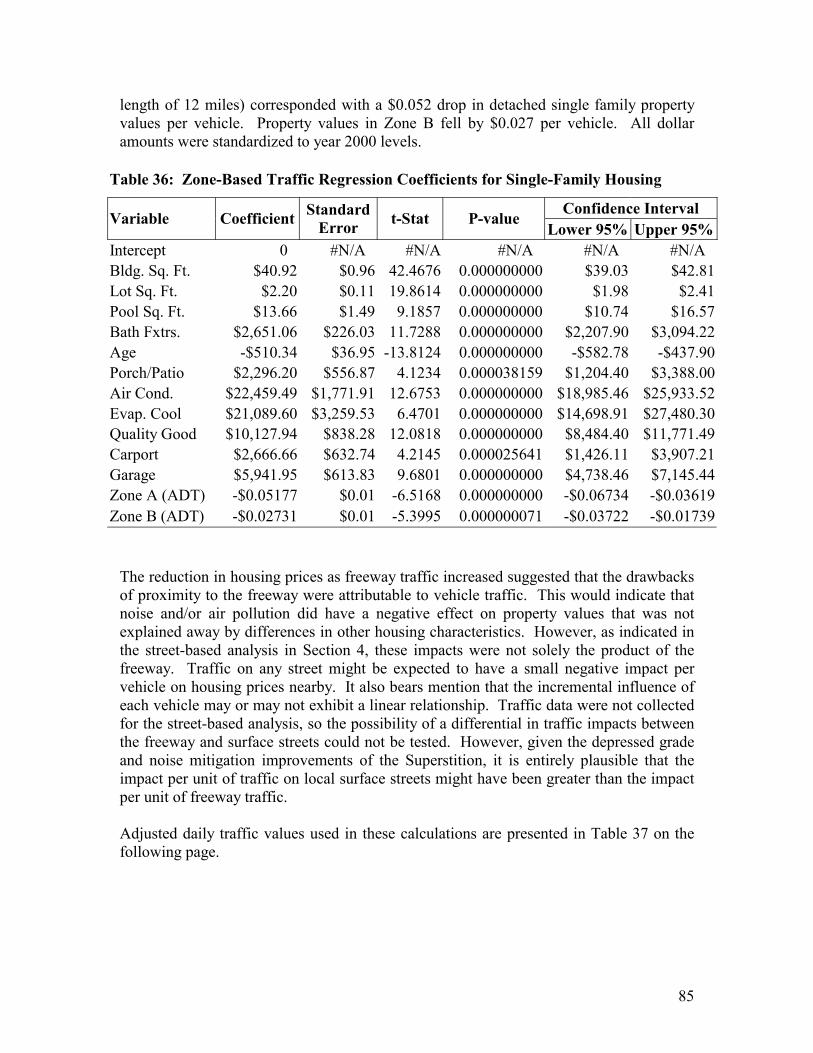
85

length of 12 miles) corresponded with a $0.052 drop in detached single family property values per vehicle. Property values in Zone B fell by $0.027 per vehicle. All dollar amounts were standardized to year 2000 levels.

Table 36: Zone-Based Traffic Regression Coefficients for Single-Family Housing

Confidence Interval Variable Coefficient Standard Error t-Stat P-value

Lower 95% Upper 95%Intercept 0 #N/A #N/A #N/A #N/A #N/A Bldg. Sq. Ft. $40.92 $0.96 42.4676 0.000000000 $39.03 $42.81Lot Sq. Ft. $2.20 $0.11 19.8614 0.000000000 $1.98 $2.41Pool Sq. Ft. $13.66 $1.49 9.1857 0.000000000 $10.74 $16.57Bath Fxtrs. $2,651.06 $226.03 11.7288 0.000000000 $2,207.90 $3,094.22Age -$510.34 $36.95 -13.8124 0.000000000 -$582.78 -$437.90Porch/Patio $2,296.20 $556.87 4.1234 0.000038159 $1,204.40 $3,388.00Air Cond. $22,459.49 $1,771.91 12.6753 0.000000000 $18,985.46 $25,933.52Evap. Cool $21,089.60 $3,259.53 6.4701 0.000000000 $14,698.91 $27,480.30Quality Good $10,127.94 $838.28 12.0818 0.000000000 $8,484.40 $11,771.49Carport $2,666.66 $632.74 4.2145 0.000025641 $1,426.11 $3,907.21Garage $5,941.95 $613.83 9.6801 0.000000000 $4,738.46 $7,145.44Zone A (ADT) -$0.05177 $0.01 -6.5168 0.000000000 -$0.06734 -$0.03619Zone B (ADT) -$0.02731 $0.01 -5.3995 0.000000071 -$0.03722 -$0.01739

The reduction in housing prices as freeway traffic increased suggested that the drawbacks of proximity to the freeway were attributable to vehicle traffic. This would indicate that noise and/or air pollution did have a negative effect on property values that was not explained away by differences in other housing characteristics. However, as indicated in the street-based analysis in Section 4, these impacts were not solely the product of the freeway. Traffic on any street might be expected to have a small negative impact per vehicle on housing prices nearby. It also bears mention that the incremental influence of each vehicle may or may not exhibit a linear relationship. Traffic data were not collected for the street-based analysis, so the possibility of a differential in traffic impacts between the freeway and surface streets could not be tested. However, given the depressed grade and noise mitigation improvements of the Superstition, it is entirely plausible that the impact per unit of traffic on local surface streets might have been greater than the impact per unit of freeway traffic. Adjusted daily traffic values used in these calculations are presented in Table 37 on the following page.

86

Table 37: US60 Average Daily Traffic Counts by Study Area Boundary

Year Start End ADT1.

1980 Exit 176: SL 101/Price Road Exit 179: Country Club Dr 11,517 1981 Exit 176: SL 101/Price Road Exit 182: Gilbert Road 5,012 1982 Exit 176: SL 101/Price Road Exit 182: Gilbert Road 26,358 1983 Exit 176: SL 101/Price Road Exit 184: Val Vista Drive 36,393 1984 Exit 176: SL 101/Price Road Exit 184: Val Vista Drive 38,003 1985 Exit 176: SL 101/Price Road Exit 188: Power Road 47,804 1986 Exit 176: SL 101/Price Road Exit 188: Power Road 54,478 1987 Exit 176: SL 101/Price Road Exit 188: Power Road 64,206 1988 Exit 176: SL 101/Price Road Exit 188: Power Road 61,600 1989 Exit 176: SL 101/Price Road Exit 188: Power Road 72,103 1990 Exit 176: SL 101/Price Road Exit 188: Power Road 97,867 1991 Exit 176: SL 101/Price Road Exit 188: Power Road 102,709 1992 Exit 176: SL 101/Price Road Exit 188: Power Road 105,605 1993 Exit 176: SL 101/Price Road Exit 188: Power Road 88,596 1994 Exit 176: SL 101/Price Road Exit 188: Power Road 101,276 1995 Exit 176: SL 101/Price Road Exit 188: Power Road 102,734 1996 Exit 176: SL 101/Price Road Exit 188: Power Road 119,861 1997 Exit 176: SL 101/Price Road Exit 188: Power Road 122,518 1998 Exit 176: SL 101/Price Road Exit 188: Power Road 119,627 1999 Exit 176: SL 101/Price Road Exit 188: Power Road 139,620 2000 Exit 176: SL 101/Price Road Exit 188: Power Road 149,304

Source: Traffic Planning Division, Arizona Department of Transportation, 2001. Notes: (1) Average daily traffic counts estimated based on average traffic counts for each segment from

start point to end point of study area boundaries – i.e. DVMT on opened sections divided total study area length.