IMF Staff Papers, Vol. 54, No. 2, 2007: Are Debt Crises Adequately ...

Are Debt Crises Adequately Defined?

ANDREA PESCATORI and AMADOU N.R. SY�

Crises on external sovereign debt are typically defined as defaults. Such adefinition adequately captures debt-servicing difficulties in the 1980s, a periodof numerous defaults on bank loans. However, defining defaults as debt crises isproblematic for the 1990s, when sovereign bond markets emerged. Not onlywere there very few defaults in the 1990s, but liquidity indicators do not playany role in explaining defaults in this period. In order to overcome the resultingdearth of data on defaults and capture the evolution of debt markets in the1990s, we define debt crises as events occurring when either a country defaultsor its bond spreads are above a critical threshold. We find that, wheninformation from bond markets is included, standard indicators—solvency andliquidity measures, as well as macroeconomic control variables—are significant.[JEL G15, G20, F3]IMF Staff Papers (2007) 54, 306–337. doi:10.1057/palgrave.imfsp.9450010

A large body of economic literature has focused on the determinants andprediction of debt crises in the aftermath of the severe global turbulence

in debt markets in the 1980s. Most studies focus on sovereign defaults andpay little attention to the more basic question, ‘‘What is a debt crisis?’’ This isnot surprising given the high frequency of sovereign defaults in this period.

�Andrea Pescatori is at the Federal Reserve Bank of Cleveland and Pompeu FabraUniversity. Amadou N.R. Sy is a senior economist at the IMF. We wish to thank the editors,an anonymous referee, Giancarlo Corsetti, Arnaud Jobert, and Enrica Detragiache as well asseminar participants at the IMF and Pompeu Fabra University for their comments. We alsothank Axel Schimmelpfennig for making available the macroeconomic data set, Peter Tran forresearch assistance, and Graham Colin-Jones for editorial suggestions.

IMF Staff PapersVol. 54, No. 2& 2007 International Monetary Fund

306

Sovereign defaults are not, however, the only possible outcome of seriousforeign debt servicing difficulties. For instance, the period starting with theMexican ‘‘crisis’’ in 1994–95 has been characterized by turbulent sovereigndebt markets and substantial IMF assistance to a number of countries. Yet,according to Moody’s Investors Service (2003), only seven rated sovereignbond issuers have defaulted on their foreign currency-denominated bondssince 1985 and all those defaults happened between 1998 and 2002. Thesurprisingly low number of sovereign bond defaults by emerging marketsovereign borrowers contrasts with the numerous defaults on bank loans inthe 1980s.We argue that defining debt crises solely as sovereign defaults does not take

into account the development of international capital markets and, notably, theadvent of the bond market for emerging market sovereign issuers. We showhow sovereign defaults have become a less reliable indicator of debt-servicingdifficulties and suggest a broader indicator of debt-servicing difficulties (debtcrisis) that takes into account turbulence in emerging bond markets.More precisely, we consider events where either there is a sovereign default

or secondary market bond spreads are higher than a critical threshold. Usingextreme value theory as well as kernel density estimation, we find that the 1,000basis point (bp) (10 percentage point) threshold corresponds to significant tailevents. In practice, market participants often view sovereign bond spreadsabove the 1,000 bp mark as a signal of turbulence in bond markets.Formally, we assume that foreign debt–servicing difficulties can be

represented by an unobservable latent variable. The standard empiricalapproach typically uses sovereign defaults as an indicator of debt-servicingdifficulties. We argue, however, that sovereign defaults are no longer theappropriate indicator for foreign debt–servicing difficulties, given their raritysince the advent of emerging market bonds. As an alternative, we propose anindicator that complements sovereign defaults with available informationfrom the sovereign bond market. This alternative framework enables us totake into account the development of the bond market for emergingeconomies in the 1990s and overcome the data limitations owing to thedearth of defaults in the 1990s.We find that typical theoretical determinants of debt-servicing

difficulties—solvency and liquidity measures, as well as macroeconomiccontrol variables—better explain our broader definition of debt crises. Incontrast, typical empirical models of debt-servicing problems fail to explaindebt crises when they are defined solely as defaults, especially in the periodafter 1994. In particular, liquidity indicators are significant in explaining ourdefinition of debt crises although they do not play any role in explainingdefaults after 1994.

I. Review of the Literature

Episodes of serious foreign debt–servicing difficulties in the 1980s in LatinAmerica and Africa have led to a large body of literature on the determinants

ARE DEBT CRISES ADEQUATELY DEFINED?

307

of debt crises.1 These studies typically define debt crises as defaults and study thefactors that lead to the nonpayment of pre-agreed debt service (Sachs, 1984).2

A related body of literature focuses on the risk of default and usesspreads between the interest rate charged to a particular country and abenchmark as a proxy for the probability of sovereign default (see Edwards,1984, for instance). As an alternative, it is possible to determine theprobability of default from spreads (see Edwards, 1984; and Duffieand Singleton, 2003) or credit default swaps (Chan-Lau, 2003). Anothermethod uses credit ratings to measure the risk of default (Kaminskyand Schumkler, 2001). Rating downgrades are therefore perceived as anincrease in the probability of default, and it is useful to focus on theintensity of rating actions or ‘‘rating crises,’’ as in Juttner and McCarthy(1998). The probability of sovereign default can also be derived froman estimated transition matrix of the default, as in Hu, Kiesel, andPerraudin (2001).Sovereign defaults are often associated with other types of financial

crises. As a result, some researchers have studied the relevance of sovereigndebt variables in explaining financial crises other than debt crises. In Radeletand Sachs (1998) and Rodrik and Velasco (2000), large reversals of capitalflows are seen as significant events, whereas in Frankel and Rose (1996);Milesi-Ferretti and Razin (1998); Berg and Pattillo (1999); and Bussiere andMulder (1999) currency crises are considered to be important. In addition,Reinhart (2002) and Sy (2004) study the relationship between defaults andcurrency crises. Debt-servicing difficulties can, however, manifest themselvesin different forms, and a number of recent studies have taken a closer look atthe definition of debt crises.

What Is a Debt Crisis?

Debt crises as sovereign defaults

Rating agencies typically focus on default events. For instance, Moody’sInvestors Service (2003) defines a sovereign issuer as in default when one ormore of the following conditions are met:

� There is a missed or delayed disbursement of interest and/or principal, evenif the delayed payment is made within the grace period, if any.

� A distressed exchange occurs, where

� the issuer offers bondholders a new security or package of securitiesthat amounts to a diminished financial obligation, such as new debtinstruments with lower coupon or par value; or

1See McDonald (1982); Edwards (1984); and Eichengreen and Mody (1998 and 1999);among others.

2For nominal domestic debt, episodes of surprise inflation have also been studied (Calvo,1988; and Alesina, Prati, and Tabellini, 1990).

Andrea Pescatori and Amadou N.R. Sy

308

� the exchange had the apparent purpose of helping the borroweravoid a ‘‘stronger’’ event of default (such as missed interest orpayment).

Similarly, Standard & Poor’s (S&P) (Chambers and Alexeeva, 2003) definesdefault as ‘‘the failure of an obligor to meet a principal or interest paymenton the due date (or within the specified grace period) contained in the originalterms of the debt issue.’’ The agency notes that:

� For local and foreign currency bonds, notes, and bills, each issuer’s debtis considered in default either when a scheduled debt-service payment is notmade on the due date or when an exchange offer of new debt contains lessfavorable terms than the original issue.

� For bank loans, when either a scheduled debt-service payment is notmade on the due date or a rescheduling of principal and/or interestis agreed to by creditors at less favorable terms than those of theoriginal loan. Such rescheduling agreements covering short- andlong-term bank debt are considered defaults even where, for legal orregulatory reasons, creditors deem forced rollover of principal to bevoluntary.3

In addition, many rescheduled sovereign bank loans are ultimatelyextinguished at a discount from their original face value. Typical dealshave included exchange offers (such as those linked to the issuance of Bradybonds), debt-equity swaps related to government privatization programs,and/or buybacks for cash. S&P considers such transactions defaults becausethey contain terms less favorable than the original obligation.Beim and Calomiris (2001) use a variety of sources to compile a list of

major periods of sovereign debt–servicing incapacity from 1800 to 1992.They examine bonds, suppliers’ credit, and bank loans to sovereign nations,but exclude intergovernmental loans, and focus on extended periods (sixmonths or more) during which all or part of interest and/or principalpayments due were reduced or rescheduled. Some of the defaults andrescheduling involved outright repudiation (a legislative or executive act ofgovernment denying liability); others were minor and announced ahead oftime in a conciliatory fashion by debtor nations.The end of each period of default or rescheduling was recorded when full

payments resumed or a restructuring was agreed to. Periods of default orrescheduling within five years of each other were combined. In the case ofa formal repudiation, its date served as the end of the period of default, andthe repudiation is noted in the notes (for example, in Cuba in 1963). Whereno clear repudiation was announced, the default was listed as persistingthrough 1992 (for example, in Bulgaria). Finally, voluntary refinancing(Colombia in 1985 and Algeria in 1992) was not included.

3For central bank currency, a default occurs when notes are converted into new currencyof less-than-equivalent face value.


309

Debt crises as large arrears

Detragiache and Spilimbergo (2001) classify an observation as a debt crisis ifeither or both of the following conditions occur:

� There are arrears of principal or interest on external obligations towardcommercial creditors (banks or bondholders) of more than 5 percent oftotal commercial debt outstanding.

� There is a rescheduling or debt restructuring agreement withcommercial creditors listed in the World Bank’s Global DevelopmentFinance.

Detragiache and Spilimbergo (2001) argue that the 5 percent minimumthreshold serves to rule out cases in which the share of debt in default isnegligible; the second criterion makes it possible to include countries that arenot technically in arrears because they reschedule or restructure theirobligations before defaulting.As a sensitivity test they also set the minimum threshold on arrears

at 15 percent of commercial debt service due. Also, because they areinterested in defaults with respect to commercial creditors, arrears orrescheduling of official debt do not count as crisis events.Finally, observations for which commercial debt is zero are excluded fromthe sample because they cannot be crisis observations based on theirdefinition.A second issue is how to distinguish the beginning of a new crisis from

the continuation of the preceding one: an episode is considered concludedwhen arrears fall below the 5 percent threshold; however, crises beginningwithin four years of the end of a previous episode are treated as acontinuation of the earlier event. In a sensitivity test, Detragiache andSpilimbergo (2001) exclude all episodes that follow the initial crisis, so thateach country has at most one crisis. Finally, because the authors seek toidentify the conditions that prompt a crisis rather than the impact of the crisison macroeconomic developments, all observations while the crisis is ongoingare excluded from the sample.These criteria identify 54 debt crises in the baseline sample. Although

events tend to cluster in the early 1980s, when most Latin American countriesand several African countries defaulted on their syndicated bank debtfollowing the borrowing boom of the 1970s, there are crises throughout thesample period. Episodes on external payment difficulties that do not result inarrears or rescheduling, such as the Mexican crisis of 1995, are not capturedby their definition of crisis. Notably, they identify only four crises in the1994–98 period.

Debt crises as large IMF loans

Manasse, Roubini, and Schimmelpfennig (2003), hereinafter referred to asMRS, argue that there are different types of sovereign debt–servicing


310

difficulties, which range from an outright default on domestic and externaldebt (Russia in 1998, Ecuador in 1999, and Argentina in 2001) tosemicoercive restructuring; that is, under the implicit threat of default(Pakistan in 1999, Ukraine in 2000, and Uruguay in 2003) and rollover/liquidity crises (Mexico in 1994–95, Korea and Thailand in 1997–98, Brazil in1999–2002, Turkey in 2001, and Uruguay in 2002) where a solvent butilliquid country is on the verge of default on its debt because of investors’unwillingness to roll over short-term debt coming to maturity, and a crisiswas in part avoided via large amounts of official support by internationalfinancial institutions as well as less coercive forms of private sectorinvolvement.MRS argue that sovereign debt–servicing difficulties (of both the

illiquidity and insolvency varieties), which were severe during the 1980sdebt crisis, have become relatively frequent phenomena again in thepast decade. As a result, the authors argue that the data in Detragiacheand Spilimbergo (2001) may exclude some incipient debt crises thatwere avoided only as a result of large-scale financial support fromofficial creditors. They therefore consider a country to be experiencing adebt crisis if:

� it is classified as being in default by S&P as previously defined, or� it has access to a large nonconcessional IMF loan in excess of 100 percentof quota.

S&P rates sovereign issuers in default if a government fails to meet aprincipal or interest payment on an external obligation on the duedate (including exchange offers, debt-equity swaps, and buyback forcash). For MRS, debt crises include not only cases of outright defaultor semicoercive restructuring, but also situations where such near-defaultwas avoided through the provision of large-scale official financing by theIMF.

Debt crises as distress events

Given the limited number of sovereign bond defaults, even under a verybroad definition such as Moody’s, Sy (2004) suggests a parallel with thedistressed-debt literature in corporate finance and defines debt crises assovereign bond distress events. The author assumes that sovereign bonds aredistressed securities when bond spreads are trading 1,000 bps or more aboveU.S. Treasury securities.Sy (2004) argues that in practice, the 1,000 bps mark for spreads is

often considered a psychological barrier by market participants. Underthe above definition of sovereign distress, the author finds 140distressed-debt events (about 14 percent of observations) from 1994to 2002 that were associated with reduced access to the sovereign bondmarket.


311

II. The 2002 Brazilian ‘‘Debt Crisis’’

Events in Brazil, in 2002, illustrate the case of a sovereign that experiencesserious debt-servicing difficulties that are not captured by sovereigndefaults.4 That year, spreads on Brazil’s external bonds rose sharply alongwith a 40 percent depreciation of the domestic currency, the real. Thesedevelopments led investors to focus on the impact of the weakness of thereal on local debt dynamics, because Brazil’s domestic government debtremained largely indexed to the U.S. dollar and domestic short-term interestrates. The heavily indexed structure of domestic government debt amplifiedthe impact of external shocks, as reflected in rising debt-service costs. Withalmost one-third of the domestic debt linked to the exchange rate, Brazil’sdebt-to-GDP ratio risked rising significantly, potentially leading to asovereign default.Against this background, Brazil reached an agreement with the IMF on

August 7 that would commit $30 billion in additional financing by the IMF,80 percent of which would be disbursed during 2003. The program relaxedthe previous net international reserve floor. In addition, it ensured fiscalsustainability over the medium term through the maintenance of a primarysurplus target of no less than 3.75 percent of GDP during 2003. The fall inBrazilian spreads triggered by the IMF program announcement quicklyreversed, however, whereas the real weakened once more to 3.15 per dollar,not far from its all-time low of 3.60 per dollar.The Brazilian authorities did not default on their large obligation in the

bond markets, an option that may have been very costly. Instead, theyreached an agreement with the IMF. However, Brazilian bond spreads wereconsistently above 1,000 bps during this period, indicating the country’s debt-servicing difficulties.

III. A Broader Definition of a Sovereign Debt Crisis

One problem with using sovereign defaults data to proxy for foreign debt–servicing difficulties relates to the dearth of observed post-1994 defaults. Infact, this period is often associated with a number of sovereign credit eventsin emerging market economies, starting with the Mexican and the Asian‘‘crises’’ (see Figure 1 and Table 1).Our concern that defaults are not a measure subtle enough to capture

changes in the nature of debt-servicing difficulties and the evolution ofinternational capital markets is shared by other authors. For instance, MRSpropose that defaults be complemented with events during which a sovereignreceives substantial IMF assistance.

4Other cases of major turbulence in debt markets that did not result in sovereign defaults(as defined by S&P) include Algeria (1999), Argentina (1995), Brazil (1995 and 1999), Coted’Ivoire (1999), Ecuador (1996 and 1998), Malaysia (1995), Nigeria (1994–96 and 1999–2002),Pakistan (2001), Turkey (2000), Ukraine (2001), and Venezuela (1994 and 1999).


312

IMF bailouts, however, do not show a structural change between the twoperiods before and after 1994. In fact, the percentage of countries receivingIMF assistance of more than 100 percent of quota has barely increased, to 4.8percent post-1994 from 4.5 percent in the previous period. Moreover, thepercentage of countries receiving IMF bailouts without defaulting has barelyincreased, to 36 percent post-1994 from 32 percent in the previous period.5 Inother words, although the MRS methodology of complementing defaultevents with IMF bailouts increases the total number of crisis events, it doesnot change the relative number of crises per period—that is, the ratio of thenumber of crisis events in the 1980s to the number of crisis events in the1990s. So we are still left with the puzzle of a drastic drop in debt crises post-1994.A possible explanation for the rarity of post-1994 default events could be

that the determinants of defaults improved in the 1990s relative to their

Figure 1. Comparison Between PesSy and Standard & Poor’s Defaults(Number of Crises)

1975 1980 1985 1990 1995 2000 20050

2

4

6

8

10

12

14

16

StdDPesSy

Source: Authors’ calculations.Note: ‘‘StdD’’ stands for defaults as defined by Standard & Poor’s defaults. ‘‘PesSy’’ refers to

events when there is either a default as defined by Standard & Poor’s or sovereign bond spreads areabove 1,000 bps (10 percentage points).

5For a broad sample of 76 countries, most of them not members of the Organization forEconomic Cooperation and Development (OECD).


313

earlier levels. If so, the factors that successfully explained defaults in the1970s and 1980s should have no problem predicting the reduced number ofdefaults in the 1990s. Our regression results show, however, that this may notbe the case. Empirical models of debt crises that worked well until the 1980scannot explain the few default events in the 1990s and instead predict agreater number of such events.It is also possible that there was a structural break between the regressors

and the dependent debt crisis variables. Such a break could be attributed tothe development of international financial markets in the 1990s. In this case,we should expect that models estimated for the 1970s and 1980s would nolonger work for the 1990s. We will, however, show that this may not be thecase, although we believe that financial development deserves closerexamination. In particular, we will attempt to show that the rapiddevelopment of the sovereign bond market for emerging economies can beused to obtain a relevant definition of debt crises.We start from the following simple consideration. The more emerging

countries have gained access to sovereign bond markets, the more they havereduced the share of bank loan debt to total debt. This means that defaultingcould be associated with both forms of debt contracts but also with only oneof them. So as a first step it seems sensible to proxy for foreign debt–servicingdifficulties using bank loans, bonds, or both types of debt instruments.A second consideration is that very few countries have defaulted on their

foreign bonds in the post-1994 period. As a result, the usual definition ofbond default must be one that is not subtle enough to capture the wide rangeof debt-servicing difficulties. The anonymous structure of bond marketsmakes renegotiation more difficult for bond contracts than bank loans.Renegotiation, however, is one of the most common credit events for othertypes of debt contracts such as bank loans and is a clear sign of debt-servicingdifficulties. In contrast, we are likely to miss important periods of debt-servicing difficulties when we restrict ourselves to the usual definition ofdefault, because of the difficulty of renegotiating bond contracts.

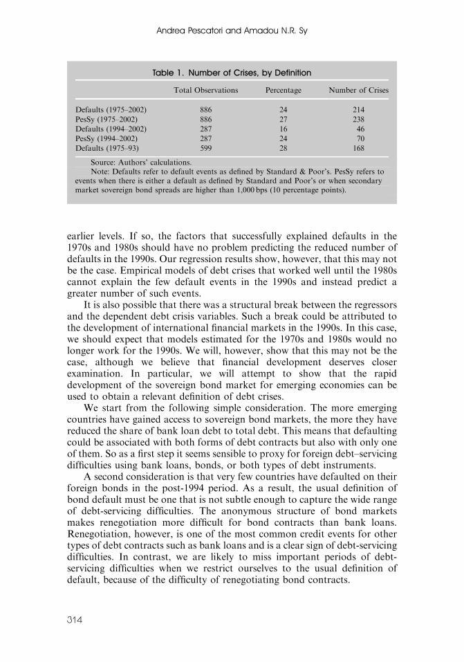
Table 1. Number of Crises, by Definition

Total Observations Percentage Number of Crises

Defaults (1975–2002) 886 24 214

PesSy (1975–2002) 886 27 238

Defaults (1994–2002) 287 16 46

PesSy (1994–2002) 287 24 70

Defaults (1975–93) 599 28 168

Source: Authors’ calculations.Note: Defaults refer to default events as defined by Standard & Poor’s. PesSy refers to

events when there is either a default as defined by Standard and Poor’s or when secondarymarket sovereign bond spreads are higher than 1,000 bps (10 percentage points).


314

In order to overcome this problem, we add a market-oriented measure ofdebt-servicing difficulties based on sovereign bond spreads: a debt crisishappens when there is either a default as defined by rating agencies (in thiscase S&P) or when the secondary market sovereign bond spreads are higherthan a critical threshold. For simplicity we will refer to debt crises defined asabove as the PesSy indicator of foreign debt–servicing difficulties.Presumably, spreads on foreign currency–denominated sovereign bonds

may be part of a broader set of measures of macroeconomic or financialconditions that characterize the ability and willingness of a sovereignborrower to repay its debt. However, there are advantages in using sovereignbond spreads, given the high frequency and quality of the data as well as thesimplicity in distinguishing among entry, continuation, and exit from a crisis.Because they provide market information, however, sovereign bond

spreads are not immune from possible overreaction from marketparticipants. Hence, bond spreads could be, at times, misaligned witheconomic fundamentals and rather reflect market participants’ overreactionsto new information about the borrower. Our crisis indicator would thereforecapture a credit event, whether it is due to economic imbalances or marketoverreactions. From a policy perspective, however, both types of events areimportant and have to be managed to avoid negative spillover effects in theeconomy. For instance, Dailami, Masson, and Padou (2005) model theprobability of sovereign default so that it (1) depends on stock of debt as wellas lagged income, (2) is highly nonlinear, and (3) can have multiple solutions.Their intuition is that by expecting a default, investors can make a defaultmore likely. However, this is true in only certain ranges for the variables andthe parameters. In particular, debt has to be large enough that increases ininterest costs can make debt service painful for the emerging marketborrower. Because of the existence of multiple equilibria, the effect ofexplanatory variables on spreads is different, depending on whichequilibrium is chosen.6

High interest rate increases also may not be attributed solely to debt-servicing problems. For instance, Garcia and Rigobon (2004) compute eventsduring which the probability of the simulated debt-to-GDP ratio exceeds athreshold deemed risky. These authors find that such ‘‘risk probabilities’’ areclosely correlated to sovereign spreads. In this type of framework, therelevant variables do not have independent paths, and high interest rates canoccur because of the co-movement observed in the variables of interest anddebt dynamics. For instance, the authors find that, as is typically the case foremerging markets, a recession can cause the fiscal accounts to deteriorate, the

6For instance, the existence of multiple equilibria gives a natural role to contagion effectsin international capital markets. The authors suggest, therefore, dividing their sample into twosubsamples: ‘‘normal’’ times and ‘‘crisis’’ periods when a particular country faces sharplyhigher spreads as a result of a debt default or currency attack, which is consistent with ourpaper. Because of the difficulty in dating crises, the authors used periods when a currency crisisoccurs.


315

real interest rate and inflation to rise, and the exchange rate to fall. Such debtdynamics worsen when the sovereign debt is dollar denominated.Figure 1 shows the number of crises signaled by defaults—as defined by

S&P—and by our crisis indicator.7 In Table 1, we divide the overall sample—which goes from 1975 to 2002—into two subsamples ranging from 1975 to1993 and from 1994 to 2002. The data show a dramatic drop in the numberof defaults to 16 percent of total observations in the 1994–2002 period, from28 percent in the 1975–93 period. In contrast, our proxy for sovereign debt–servicing difficulties indicates more stable behavior with a proportion of 24percent of debt crises in the 1994–2002 period.In order to formalize the previous argument and compare the two

definitions of debt crises—namely, sovereign defaults and the indicator ofdebt-servicing difficulties (PesSy), we assume that there is an unobservablestate of nature that corresponds to a country experiencing foreign debt–servicing difficulties. These foreign debt–servicing difficulties are notobservable per se by creditors,8 but the observation of some indicators,such as the inability of a sovereign to repay its debt, may be used to infer thetrue state of affairs.We assume the existence of a latent variable, y�, that represents foreign

debt–servicing difficulties for a particular country. The underlying responsevariable is then defined by a regression relationship:

y�t ¼ b0xt þ ut: (1Þ

The next step is to link the latent variable to some observable variables.The standard approach is to use sovereign defaults as an indicator of debt-servicing difficulties. Thus, the default indicator I is defined as

It ¼1 if y�t40;

0 otherwise:

((2Þ

In contrast, it is possible to use the information from the bond marketand assume that a sovereign credit event is also signaled when a country’sbond spreads, s, cross a threshold, t. We define the spreads in excess of thethreshold as

st � tt ¼ hðy�t Þ;

where h is any strictly increasing Borel function defined on the y� probabilityspace, such that h(0)¼ 0. We then construct a binary indicator related to the

7The data for spreads start from 1994 so that the two variables overlap in the periodbefore.

8It is private information for the sovereign debtor.


316

latent variable, S, such as

St ¼1 if st � tt40;

0 otherwise;

(or

1 if Y�t40;

0 otherwise:

((3Þ

We propose a more general model combining the default indicator withthe spreads-based indicator, so that a debt crisis occurs when either a defaultexists or bond spreads are above a threshold. In this case, the latent variableis linked to a bivariate observable variable, yt(It, St), such that

~yt ¼

ð1; 1Þ

ð1; 0Þ if y�t40;

ð0; 1Þ

ð0; 0Þ otherwise;

8>>>>><>>>>>:

(4aÞ

which can be reduced to the following univariate variable:

yt ¼0 if ~y ¼ ð0; 0Þ;

1 otherwise:

((4bÞ

If specification (4a)–(4b) is the ‘‘true’’ model, then models (2) and (3) aremisspecified. Furthermore, using model (2) implies assuming that theconditional probability is unconditional. From model (2) we get

PðIt ¼ 1Þ ¼ Pðy�t40Þ ¼ 1� Fð�b0xtÞ:

From model (4) we have

1� Fð�b0xtÞ ¼ Pðy�t40Þ ¼ PðIt ¼ 1=St ¼ 0Þ:

Until the beginning of the 1990s, conditioning on S¼ 0 was consistentwith the fact that most emerging economies did not have access tointernational bond markets. In contrast, it seems reasonable to assume thatsuch a specification may miss the information given by bond markets,because emerging markets are gradually using sovereign bonds as a majorsource of funding. We therefore complement the typical default indicatorwith an indicator that uses the information from international bond markets.As an alternative, our proposed indicator assumes that there has been

historically no structural break between the latent variable and thecovariates. Rather, there have been difficulties in choosing a properindicator of an unobservable dependent variable. In the next section, weuse statistical methods to estimate the critical threshold for bond spreads, t.


317

Estimating the Threshold for Bond Spreads Using Extreme Value Theory

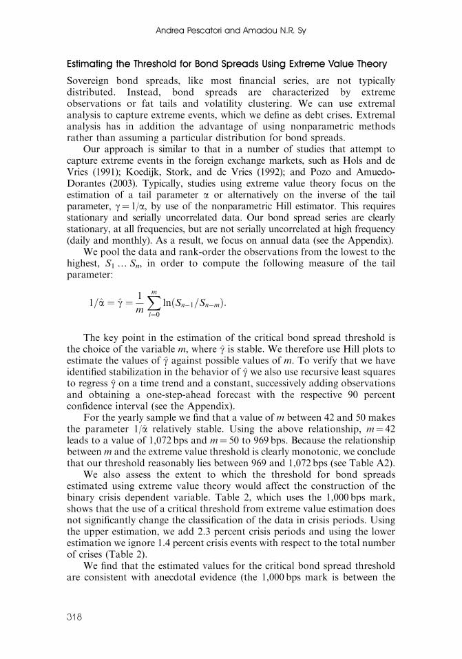
Sovereign bond spreads, like most financial series, are not typicallydistributed. Instead, bond spreads are characterized by extremeobservations or fat tails and volatility clustering. We can use extremalanalysis to capture extreme events, which we define as debt crises. Extremalanalysis has in addition the advantage of using nonparametric methodsrather than assuming a particular distribution for bond spreads.Our approach is similar to that in a number of studies that attempt to

capture extreme events in the foreign exchange markets, such as Hols and deVries (1991); Koedijk, Stork, and de Vries (1992); and Pozo and Amuedo-Dorantes (2003). Typically, studies using extreme value theory focus on theestimation of a tail parameter a or alternatively on the inverse of the tailparameter, g¼ 1/a, by use of the nonparametric Hill estimator. This requiresstationary and serially uncorrelated data. Our bond spread series are clearlystationary, at all frequencies, but are not serially uncorrelated at high frequency(daily and monthly). As a result, we focus on annual data (see the Appendix).We pool the data and rank-order the observations from the lowest to the

highest, S1ySn, in order to compute the following measure of the tailparameter:

1=a ¼ g ¼ 1

m

Xmi¼0lnðSn�1=Sn�mÞ:

The key point in the estimation of the critical bond spread threshold isthe choice of the variable m, where g is stable. We therefore use Hill plots toestimate the values of g against possible values of m. To verify that we haveidentified stabilization in the behavior of g we also use recursive least squaresto regress g on a time trend and a constant, successively adding observationsand obtaining a one-step-ahead forecast with the respective 90 percentconfidence interval (see the Appendix).For the yearly sample we find that a value of m between 42 and 50 makes

the parameter 1/a relatively stable. Using the above relationship, m¼ 42leads to a value of 1,072 bps and m¼ 50 to 969 bps. Because the relationshipbetween m and the extreme value threshold is clearly monotonic, we concludethat our threshold reasonably lies between 969 and 1,072 bps (see Table A2).We also assess the extent to which the threshold for bond spreads

estimated using extreme value theory would affect the construction of thebinary crisis dependent variable. Table 2, which uses the 1,000 bps mark,shows that the use of a critical threshold from extreme value estimation doesnot significantly change the classification of the data in crisis periods. Usingthe upper estimation, we add 2.3 percent crisis periods and using the lowerestimation we ignore 1.4 percent crisis events with respect to the total numberof crises (Table 2).We find that the estimated values for the critical bond spread threshold

are consistent with anecdotal evidence (the 1,000 bps mark is between the


318

lower and upper estimate) and do not significantly affect our dependentbinary variable. In the next section, we take a second look at the data usingkernel density estimation.

Estimating the Threshold for Bond Spreads Using a Kernel DensityEstimation

As discussed above, sovereign bond spread series do not follow a typicaldistribution. In this section, we use kernel density estimation as an alternativeto extremal analysis to estimate the key features of our sovereign bond spreadseries. We are particularly interested in the possible existence of modesaround high spread values. If bond spreads tend to cluster around some lowand large observations, then we can use these values to define ‘‘tranquil’’ and‘‘crisis’’ periods.Intuitively, whenever spreads are close to a limit that cannot be passed

smoothly, the observations will concentrate around it until the limit is finallypassed or the surging pressure reduced. Because the body of the distributionlies to the left of our threshold we also should expect that the mode is slightlyon the left (see Section II of the Appendix for an illustration).We analyze both yearly and daily data. In this case, the presence of

autocorrelation, which is very strong for daily data, does not spoil the results.In a univariate sample that is not identically and independently distributedbut autocorrelated, we expect its histogram to show a mode for each relevantturning point, and in this case around tranquil and crisis periods. In addition,there may be smaller modes for very high spreads that have been peaks orturning points for some countries.The kernel density estimation confirms the assumption that there is a

mode for tranquil and crisis periods. In particular, we find a mode around1,000 bps for both daily and yearly data. Because the yearly data are notcorrelated, we also fit a gamma and a Weibul distribution (an extreme valuedistribution) to estimate the 90th percentile.9 We choose the 90th percentileas a proxy for extreme events. Our results indicate that the 1,000 bp threshold

Table 2. Extreme Value Theory (EVT) vs. 1,000 bps Thresholds(Sample: 1994–2002)

Matching EVT Adding EVT Crossing Out Total

Total number [211, 213] [5, 0] [0, 3] 216

As percentage [0.98, 0.99] [0, 0.023] [0, 0.014] 1

Source: Authors’ calculations.Note: The abbreviation bps denotes basis points (hundredths of a percentage).

9We do not estimate the 90th percentile for daily data because of the presence of strongmultimodality.


319

is inside the 95 percent confidence bands for the 90th percentile of the fitteddistribution (Table 3).

Psychological/Market Threshold

Sovereign bond market participants typically consider the 1,000 bps mark forspreads a critical psychological threshold. Indeed, discussions with marketparticipants suggest that price quotes are increasingly based on expectedrecovery values in case of a default, when bond spreads cross the 1,000 bpsmark.For instance, Altman (1998) defines distressed securities as those publicly

held and traded debt and equity securities of firms that have defaulted ontheir debt obligations and/or have filed for protection under Chapter 11 ofthe U.S. Bankruptcy Code. Under a more comprehensive definition, Altman(1998) considers that distressed securities would include those publicly helddebt securities selling at sufficiently discounted prices so as to be yielding,should they not default, a significant premium of a minimum of 1,000 bps(or 10 percent) over comparable U.S. Treasury securities. Similarly, somemarket participants consider securities to have reached distressed levels whenthey have lost one-third of their value.The sections above corroborate the existence of a 1,000 bps market

threshold. Table 4 presents the debt crisis dates for both the standard defaultdefinition (S&P) and our broader indicator (PesSy) in the period 1994–2002.Prior to 1994, both indicators coincide, because the bond market for emerg-ing economies was not developed. In the next sections, we use the frameworkdeveloped above to estimate econometric models of debt crises.

IV. Defaults vs. Market-Based Definition of Debt Crises (PesSy)

In this section, we investigate whether the typical determinants of debt crisesfound in the literature are significant when we broaden the definition of debtcrises to include information from the bond markets. We also study how well

Table 3. Thresholds for Bond Spreads from Kernel Density Estimations

Estimated 90th Percentile—95 Percent Confidence Interval

Gamma distribution 1,036.52 [980.55, 1,093.85]

Weibul distribution 978.82 [795.10, 1,248.05]

Percentile Corresponding to 1,000 bps

Gamma distribution 0.88

Weibul distribution 0.91

Source: Authors’ calculations.Note: bps=basis points.


320

these explanatory variables forecast our proposed broader definition of debtcrises. As an illustration, we also repeat the same exercise for sovereign defaults.

Baseline Regressions, 1975–2002

The theoretical and empirical literature has highlighted a number of variablesthat help predict sovereign defaults. The explanatory variables usuallyinclude (1) liquidity indicators (short-term debt over reserves; or short-termdebt, debt service due, and reserves separately); (2) variables that measure themagnitude and structure of external debt; and (3) macroeconomic control

Table 4. Debt Crises Dates, 1994–2002

Country PesSy1 Default (S&P)

Algeria 1994–96, 1999 1994–96

Argentina 1995, 2001–02 2001–02

Brazil 1994–95, 1999, 2002 1994

Cote d’Ivoire 1994–2002 1994–98, 2000–02

Chile No crisis No crisis

China No crisis No crisis

Colombia No crisis No crisis

Dominican Rep. 1994 1994

Ecuador 1994–96, 1998–2002 1994–95, 1999–2000

Egypt No crisis No crisis

El Salvador No crisis No crisis

Hungary No crisis No crisis

Indonesia 1998–2000, 2002 1998–2000, 2002

Korea No crisis No crisis

Lebanon No crisis No crisis

Malaysia 1995 No crisis

Mexico 1995 No crisis

Morocco No crisis No crisis

Nigeria 1994–96, 1999–2002 No crisis

Pakistan 1998–99, 2001 1998–99

Panama 1994–96 1994–96

Peru 1994–97 1994–97

Philippines No crisis No crisis

Poland 1994 1994

Russia 1994–2000 1994–2000

South Africa No crisis No crisis

Thailand No crisis No crisis

Tunisia No crisis No crisis

Turkey No crisis No crisis

Ukraine 1998–2001 1998–2000

Uruguay No crisis No crisis

Venezuela 1994–97,1999, 2002 1995–97

Source: Standard & Poor’s and authors’ calculations.Note: S&P=Standard & Poor’s.1Default or bond spreads above 1,000 bps.


321

variables, such as measures of openness and real exchange rate over-valuation.For instance, MRS, after reviewing the empirical and theoretical

literature on debt crises, emphasize the following determinants of debt crises:

� solvency measures, such as public and external debt relative to capacity topay;

� liquidity measures, such as short-term external debt and external debtservice, possibly in relation to reserves or exports;

� currency crisis (early-warning systems) variables;� external volatility and volatility in economic policy measures;� macroeconomic control variables, such as growth, inflation, and exchangerate; and

� political and institutional variables that capture a country’s willingness topay.

We follow the literature and use the typical determinants of debt crises asexplanatory variables. In fact, we assume that standard explanatory variablesare the correct ones in predicting debt crises but that indicators of debt crisesmay be inaccurate.As a first descriptive step we use the whole sample from 1975 to 2002. In

Table 5, we show the estimation results for the standard framework—wherethe sovereign default variable is the indicator variable for debt crises. InTable 6, we present the results for the alternative market-based indicator(PesSy).10

We find that, for the 1975–2002 period, solvency measures (total debt overGDP) and liquidity indicators (short-term debt over reserves) are statisticallysignificant in explaining debt crises, independently of how they are defined.However, the liquidity indicator (short-term debt over reserves) plays a moreimportant role; inflation is not significant when the market-based indicator isused. Other macroeconomic control variables—in particular, real growth rate,inflation, and real exchange rate overvaluation—are also important inexplaining crises, as is a measure of openness (imports plus exports overGDP). All regressors are significant at 5 percent in both specifications (with orwithout inflation) and enter with the right sign.Finally, a comparison of the Wald statistics suggests that standard macro

variables, except for inflation, provide a better explanation of debt crises asdefined by the market-based indicator (PesSy).

10Our logit methodology is quite standard but suits our purpose well. Recent researchillustrates how the relationship between the explanatory variables used to predict debt crisescan be dynamic and nonlinear. For instance, in Garcia and Rigobon (2004), episodes wherethe debt-to-GDP ratio is higher than a critical threshold are the relevant events. However,their model exploits the covariance of stochastic debt and other macro variables by using avector autoregressions (VAR) methodology. Similarly, in Dailami, Masson, and Padou(2005), spreads in normal and (currency) crisis periods are used but in a highly nonlinearmodel with multiple equilibria, which necessitates the use of a pooled mean group estimator.


322

Out-of-Sample Comparisons

Typically, model estimation attempts to find the explanatory variables thatbetter explain a particular dependent variable. In this section, we take theexplanatory variables as given and focus instead on finding the better proxyfor the unobservable dependent variable, debt-servicing difficulties. We showthat debt-servicing difficulties are better captured when we use informationfrom both sovereign defaults and bond markets.The two indicators of debt-servicing difficulties coincide in the period

before 1994—that is, before the advent of the emerging bond market—anddiffer only afterward. We therefore estimate the model for the period 1975–93 to forecast debt crises in 1994–2002 (out-of-sample). We then compare ourforecasts with actual proxies of the dependent variable in 1994–2002. We findthat forecasted debt crises are statistically closer to the actual observations ofour market-based indicator than sovereign defaults.Estimation results for the subsample 1975–93 are shown in Table 7.11 All

variables are significant except for inflation, and the Wald statistic iscomparable to the values obtained earlier. The solvency (total debt overGDP) and liquidity (short-term debt over reserves) variables play a biggerrole compared with the results obtained using the whole sample with thedefault indicator. The opposite is true for inflation, which is nowinsignificant. In other words, the estimation results for the 1975–93 periodseem to be comparable to the results obtained with the market-basedindicator for the whole sample period (1975–2002) (compare Table 7 to Table6 and Table 5).Given that we estimate a binary variable model, we follow the early-

warning indicator literature for currency crises and estimate the number ofmatched crises (A), false alarms (B), missing crises (C), and matched tranquilperiods (D).12

In this framework, a signal is sent whenever the estimated probability of acrisis crosses a given threshold, T. Typically, the threshold is set to be equalto the unconditional probability of a crisis occurring. Because we are tryingto match the crisis events, there is no clear reason for setting T to theunconditional probability, and we instead leave the variables A, B, C, and Das a function of the threshold T, which is optimally determined. In order tocalculate the optimal threshold value for issuing a warning, T �, we minimizethe following noise-to-signal ratio: L(T)¼B(T)/A(T)þC(T)/D(T). Becausethe standard error for the forecasts is quite high, we estimate the values forT� using a bootstrapping method, and hence for A(T�), B(T�), C(T�), D(T�),and L(T�). Table 8 shows the ratios for ‘‘Matched Crises over Total Crises,’’A(T�)/[A(T�)þC(T�)], and ‘‘False Alarms over Tranquil Periods,’’ B(T�)/[B(T�)þD(T�)].

11In order not to give an advantage or penalize the PesSy indicator, we use the baselinemodel with inflation among regressors.

12For a review of the method used here, we refer the reader to Berg and Pattillo (1999).


323

The results, shown in Table 8, indicate that, in terms of matched crises, thetypical determinants of debt crises forecast better the market-based indicator(PesSy) than sovereign defaults. This is not really surprising given that there aremore debt crises under the market-based definition than defaults. Hence, for amore conclusive answer and to aggregate the previous results, we introduce a

Table 5. Regression Results Using Default Definition, 1975–2002

S&P Default

Definition Coeff. Z P>|z|

95 Percent

CI Coeff. Z P>|z|

95 Percent

CI

Openness �0.05 �3.14 0.00 �0.08 �0.02 �0.05 �3.08 0.00 �0.07 �0.02Overvaluation 0.01 3.40 0.00 0.01 0.02 0.01 3.37 0.00 0.00 0.02

Total debt

over GDP

0.06 3.57 0.00 0.03 0.09 0.06 3.56 0.00 0.03 0.09

Short-term

debt over

reserves

0.19 2.07 0.04 0.01 0.36 0.19 2.05 0.04 0.01 0.37

Real growth

rate

�0.08 �2.49 0.01 �0.15 �0.02 �0.08 �2.35 0.02 �0.15 �0.01

Inflation 0.00 2.67 0.01 0.00 0.00

Constant �1.94 �2.43 0.02 �3.51 �0.37 �2.09 �2.48 0.01 �3.74 �0.44Wald w2 (5)and (6)

44.0 46.1

Source: Authors’ calculations.Note: GEE logit population-averaged model, correlation exchangeable, Huber-White

estimator. 567 observations. CI refers to the confidence intervals.

Table 6. Regression Results Using PesSy Indicator, 1975–2002

PesSy

Indicator Coeff. Z P>|z|

95 Percent

CI Coeff. Z P>|z|

95 Percent

CI

Openness �0.03 �2.06 0.04 �0.07 0.00 �0.03 �2.15 0.03 �0.06 0.00

Overvaluation 0.01 2.75 0.01 0.00 0.02 0.01 2.41 0.02 0.00 0.01

Total debt

over GDP

0.06 4.26 0.00 0.03 0.09 0.06 4.46 0.00 0.03 0.09

Short-term

debt over

reserves

0.30 2.50 0.01 0.06 0.53 0.30 2.47 0.01 0.06 0.53

Real growth

rate

�0.09 �2.61 0.01 �0.17 �0.02 �0.08 �2.29 0.02 �0.15 �0.01

Inflation 0.00 1.25 0.21 0.00 0.01


48.0 45.4


estimation. 567 observations. CI refers to confidence intervals.


324

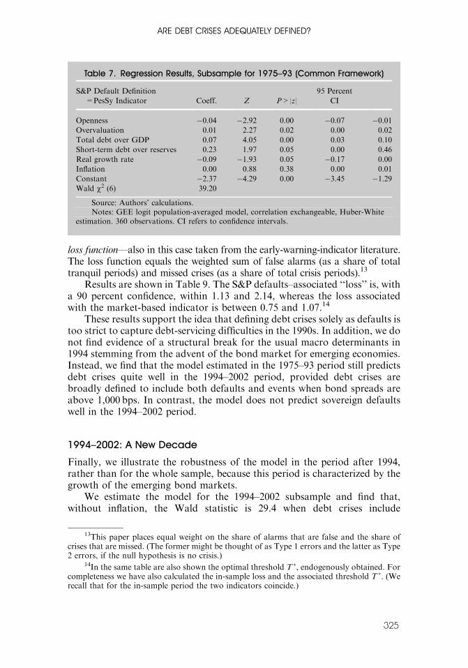
loss function—also in this case taken from the early-warning-indicator literature.The loss function equals the weighted sum of false alarms (as a share of totaltranquil periods) and missed crises (as a share of total crisis periods).13

Results are shown in Table 9. The S&P defaults–associated ‘‘loss’’ is, witha 90 percent confidence, within 1.13 and 2.14, whereas the loss associatedwith the market-based indicator is between 0.75 and 1.07.14

These results support the idea that defining debt crises solely as defaults istoo strict to capture debt-servicing difficulties in the 1990s. In addition, we donot find evidence of a structural break for the usual macro determinants in1994 stemming from the advent of the bond market for emerging economies.Instead, we find that the model estimated in the 1975–93 period still predictsdebt crises quite well in the 1994–2002 period, provided debt crises arebroadly defined to include both defaults and events when bond spreads areabove 1,000 bps. In contrast, the model does not predict sovereign defaultswell in the 1994–2002 period.

1994–2002: A New Decade

Finally, we illustrate the robustness of the model in the period after 1994,rather than for the whole sample, because this period is characterized by thegrowth of the emerging bond markets.We estimate the model for the 1994–2002 subsample and find that,

without inflation, the Wald statistic is 29.4 when debt crises include

Table 7. Regression Results, Subsample for 1975–93 (Common Framework)

S&P Default Definition

=PesSy Indicator Coeff. Z P>|z|

95 Percent

CI

Openness �0.04 �2.92 0.00 �0.07 �0.01Overvaluation 0.01 2.27 0.02 0.00 0.02

Total debt over GDP 0.07 4.05 0.00 0.03 0.10

Short-term debt over reserves 0.23 1.97 0.05 0.00 0.46

Real growth rate �0.09 �1.93 0.05 �0.17 0.00

Inflation 0.00 0.88 0.38 0.00 0.01

Constant �2.37 �4.29 0.00 �3.45 �1.29Wald w2 (6) 39.20

Source: Authors’ calculations.Notes: GEE logit population-averaged model, correlation exchangeable, Huber-White

estimation. 360 observations. CI refers to confidence intervals.

13This paper places equal weight on the share of alarms that are false and the share ofcrises that are missed. (The former might be thought of as Type 1 errors and the latter as Type2 errors, if the null hypothesis is no crisis.)

14In the same table are also shown the optimal threshold T �, endogenously obtained. Forcompleteness we have also calculated the in-sample loss and the associated threshold T �. (Werecall that for the in-sample period the two indicators coincide.)


325

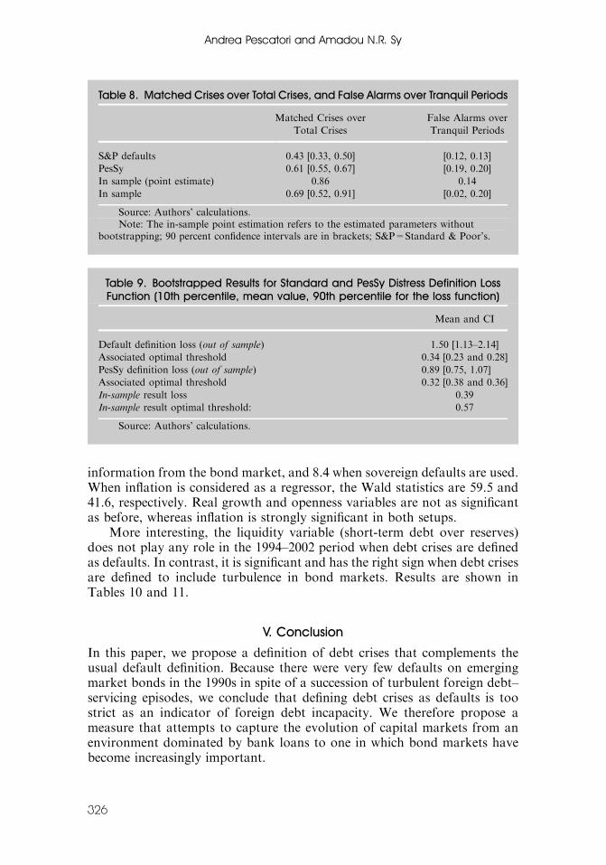
information from the bond market, and 8.4 when sovereign defaults are used.When inflation is considered as a regressor, the Wald statistics are 59.5 and41.6, respectively. Real growth and openness variables are not as significantas before, whereas inflation is strongly significant in both setups.More interesting, the liquidity variable (short-term debt over reserves)

does not play any role in the 1994–2002 period when debt crises are definedas defaults. In contrast, it is significant and has the right sign when debt crisesare defined to include turbulence in bond markets. Results are shown inTables 10 and 11.

V. Conclusion

In this paper, we propose a definition of debt crises that complements theusual default definition. Because there were very few defaults on emergingmarket bonds in the 1990s in spite of a succession of turbulent foreign debt–servicing episodes, we conclude that defining debt crises as defaults is toostrict as an indicator of foreign debt incapacity. We therefore propose ameasure that attempts to capture the evolution of capital markets from anenvironment dominated by bank loans to one in which bond markets havebecome increasingly important.

Table 8. Matched Crises over Total Crises, and False Alarms over Tranquil Periods

Matched Crises over

Total Crises

False Alarms over

Tranquil Periods

S&P defaults 0.43 [0.33, 0.50] [0.12, 0.13]

PesSy 0.61 [0.55, 0.67] [0.19, 0.20]

In sample (point estimate) 0.86 0.14

In sample 0.69 [0.52, 0.91] [0.02, 0.20]

Source: Authors’ calculations.Note: The in-sample point estimation refers to the estimated parameters without

bootstrapping; 90 percent confidence intervals are in brackets; S&P=Standard & Poor’s.

Table 9. Bootstrapped Results for Standard and PesSy Distress Definition LossFunction (10th percentile, mean value, 90th percentile for the loss function)

Mean and CI

Default definition loss (out of sample) 1.50 [1.13–2.14]

Associated optimal threshold 0.34 [0.23 and 0.28]

PesSy definition loss (out of sample) 0.89 [0.75, 1.07]

Associated optimal threshold 0.32 [0.38 and 0.36]

In-sample result loss 0.39

In-sample result optimal threshold: 0.57

Source: Authors’ calculations.


326

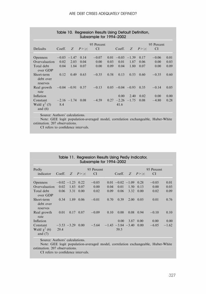
Table 10. Regression Results Using Default Definition,Subsample for 1994–2002

Defaults Coeff. Z P>|z|

95 Percent

CI Coeff. Z P>|z|

95 Percent

CI

Openness �0.03 �1.47 0.14 �0.07 0.01 �0.03 �1.39 0.17 �0.06 0.01

Overvaluation 0.02 2.03 0.04 0.00 0.03 0.01 1.87 0.06 0.00 0.03

Total debt

over GDP

0.04 1.84 0.07 0.00 0.09 0.04 1.80 0.07 0.00 0.09

Short-term

debt over

reserves

0.12 0.49 0.63 �0.35 0.58 0.13 0.53 0.60 �0.35 0.60

Real growth

rate

�0.04 �0.91 0.37 �0.13 0.05 �0.04 �0.93 0.35 �0.14 0.05

Inflation 0.00 2.40 0.02 0.00 0.00

Constant �2.16 �1.74 0.08 �4.59 0.27 �2.26 �1.75 0.08 �4.80 0.28

Wald w2 (5)and (6)

8.4 41.6


estimation. 207 observations.CI refers to confidence intervals.

Table 11. Regression Results Using PesSy Indicator,Subsample for 1994–2002

PesSy

indicator Coeff. Z P>|z|

95 Percent

CI Coeff. Z P>|z|

95 Percent

CI

Openness �0.02 �1.23 0.22 �0.05 0.01 �0.02 �1.09 0.28 �0.05 0.01

Overvaluation 0.02 1.83 0.07 0.00 0.04 0.01 1.50 0.13 0.00 0.03

Total debt

over GDP

0.06 3.31 0.00 0.02 0.09 0.06 3.32 0.00 0.02 0.09

Short-term

debt over

reserves

0.34 1.89 0.06 �0.01 0.70 0.39 2.00 0.05 0.01 0.76

Real growth

rate

0.01 0.17 0.87 �0.09 0.10 0.00 0.08 0.94 �0.10 0.10

Inflation 0.00 3.87 0.00 0.00 0.00


29.4 59.5


estimation. 207 observations.CI refers to confidence intervals.


327

We define debt crises as events either when there is a default or whensecondary-market bond spreads are higher than a critical threshold. Weshow, using extreme value theory and kernel density estimation, that athreshold of 1,000 bps does represent a statistically significant criticalthreshold. In practice, this threshold is often used by market participants.We find that our definition accurately captures debt-servicing difficulties

in the period from 1975 to 2002 and captures such difficulties better than theusual default definition, especially in the period after 1994. More precisely,we find that when our definition is used, the typical determinants of bankloan defaults in the 1980s still have predictive power for debt-servicingdifficulties—on both bank loans and bonds—in the period from 1994 to2002.15 In contrast, the standard definition of default implies much worseout-of-sample performance. In addition, we find that liquidity indicators aresignificant in explaining our definition of debt crises, although they do notplay any role in explaining defaults in the period from 1994 to 2002.

APPENDIX

Extreme-Value-Theory Approach

Like most financial data, emerging market bond spread series are not typicallydistributed but rather characterized by higher skewness, volatility clustering, andkurtosis (fat tails) than a typical distribution (see Mauro, Sussman, and Yafeh,2002). Such fat tails indicate that extreme observations are more frequent than undera normal distribution.Rather than assuming a particular distributional model, which would capture

these fat tails, we use extremal analysis to characterize the distribution of bondspreads and identify extreme observations (see Koedijk, Schafgans, and de Vries,1990; Hols and de Vries, 1991; Koedijk, Stork, and de Vries, 1992; and Pozo andAmuedo-Dorantes, 2003). Using extremal analysis, we can estimate the value of thetail parameter (a) or alternately its inverse (g¼ 1/a) to make inferences about thedistribution of bond spreads. The tail parameter takes on values between 0 and 2when the distribution of bond spreads is in the domain of attraction of a stable law;it takes on values of 2 and above for the Student-t and specific ARCH cases.Following Pozo and Amuedo-Dorantes (2003) and Koedijk, Stork, and de Vries

(1992), we use the nonparametric Hill estimator to estimate the value of the tailparameter a for our bond spread series. The Hill estimator requires that the bondspread series be stationary and serially uncorrelated.We use the Hill estimator because our bond spreads series are stationary (Dickey-

Fuller and Phillips-Perron tests results not shown) and serially uncorrelated exceptfor a few cases. To test for serial correlation we use the Ljung-Box Q-statistics for upto eight-order serial correlation. For annual data, the null hypothesis of no serialcorrelation is rejected for only four out of 31 countries (Table A.1). The countries arethose for which our bond spread sample is very small.

15By pooling the data, we obtain more precise estimates for the tail parameter a but at thecost of constraining its value to be the same for all countries (see Pozo and Amuedo-Dorantes,2003).


328

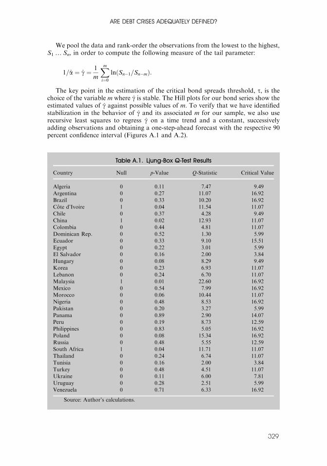
We pool the data and rank-order the observations from the lowest to the highest,S1ySn, in order to compute the following measure of the tail parameter:

1=a ¼ g ¼ 1

m

Xmi¼0lnðSn�1=Sn�mÞ:

The key point in the estimation of the critical bond spreads threshold, t, is thechoice of the variable m where g is stable. The Hill plots for our bond series show theestimated values of g against possible values of m. To verify that we have identifiedstabilization in the behavior of g and its associated m for our sample, we also userecursive least squares to regress g on a time trend and a constant, successivelyadding observations and obtaining a one-step-ahead forecast with the respective 90percent confidence interval (Figures A.1 and A.2).

Table A.1. Ljung-Box Q-Test Results

Country Null p-Value Q-Statistic Critical Value

Algeria 0 0.11 7.47 9.49

Argentina 0 0.27 11.07 16.92

Brazil 0 0.33 10.20 16.92

Cote d’Ivoire 1 0.04 11.54 11.07

Chile 0 0.37 4.28 9.49

China 1 0.02 12.93 11.07

Colombia 0 0.44 4.81 11.07

Dominican Rep. 0 0.52 1.30 5.99

Ecuador 0 0.33 9.10 15.51

Egypt 0 0.22 3.01 5.99

El Salvador 0 0.16 2.00 3.84

Hungary 0 0.08 8.29 9.49

Korea 0 0.23 6.93 11.07

Lebanon 0 0.24 6.70 11.07

Malaysia 1 0.01 22.60 16.92

Mexico 0 0.54 7.99 16.92

Morocco 0 0.06 10.44 11.07

Nigeria 0 0.48 8.53 16.92

Pakistan 0 0.20 3.27 5.99

Panama 0 0.89 2.90 14.07

Peru 0 0.19 8.73 12.59

Philippines 0 0.83 5.05 16.92

Poland 0 0.08 15.34 16.92

Russia 0 0.48 5.55 12.59

South Africa 1 0.04 11.71 11.07

Thailand 0 0.24 6.74 11.07

Tunisia 0 0.16 2.00 3.84

Turkey 0 0.48 4.51 11.07

Ukraine 0 0.11 6.00 7.81

Uruguay 0 0.28 2.51 5.99

Venezuela 0 0.71 6.33 16.92

Source: Author’s calculations.


329

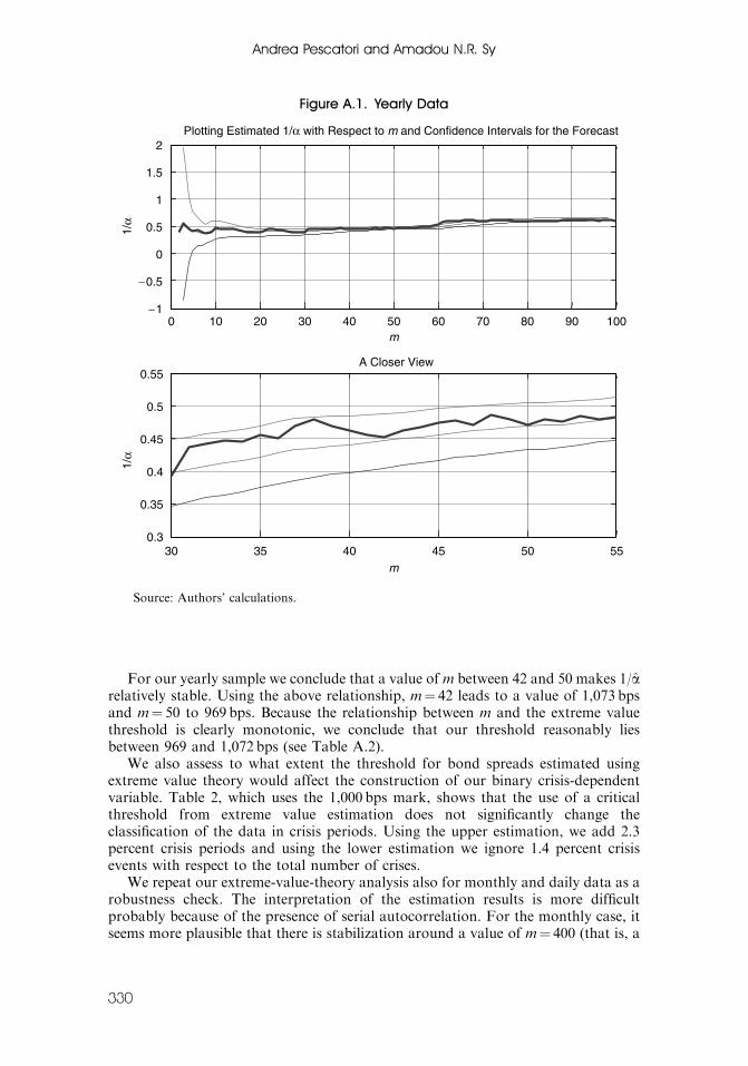
For our yearly sample we conclude that a value of m between 42 and 50 makes 1/arelatively stable. Using the above relationship, m¼ 42 leads to a value of 1,073 bpsand m¼ 50 to 969 bps. Because the relationship between m and the extreme valuethreshold is clearly monotonic, we conclude that our threshold reasonably liesbetween 969 and 1,072 bps (see Table A.2).We also assess to what extent the threshold for bond spreads estimated using

extreme value theory would affect the construction of our binary crisis-dependentvariable. Table 2, which uses the 1,000 bps mark, shows that the use of a criticalthreshold from extreme value estimation does not significantly change theclassification of the data in crisis periods. Using the upper estimation, we add 2.3percent crisis periods and using the lower estimation we ignore 1.4 percent crisisevents with respect to the total number of crises.We repeat our extreme-value-theory analysis also for monthly and daily data as a

robustness check. The interpretation of the estimation results is more difficultprobably because of the presence of serial autocorrelation. For the monthly case, itseems more plausible that there is stabilization around a value of m¼ 400 (that is, a

Figure A.1. Yearly Data

0 10 20 30 40 50 60 70 80 90 100− 1

− 0.5

0

0.5

1

1.5

2Plotting Estimated 1/α with Respect to m and Confidence Intervals for the Forecast

30 35 40 45 50 550.3

0.35

0.4

0.45

0.5

0.55A Closer View

1/α

1/α

m

m



330

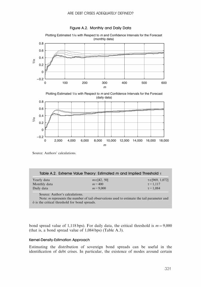
bond spread value of 1,118 bps). For daily data, the critical threshold is m¼ 9,000(that is, a bond spread value of 1,084 bps) (Table A.3).

Kernel-Density-Estimation Approach

Estimating the distribution of sovereign bond spreads can be useful in theidentification of debt crises. In particular, the existence of modes around certain

Figure A.2. Monthly and Daily Data

0 100 200 300 400 500 600– 0.2

0

0.2

0.4

0.6

0.8

Plotting Estimated 1/α with Respect to m and Confidence Intervals for the Forecast (monthly data)

Plotting Estimated 1/α with Respect to m and Confidence Intervals for the Forecast (daily data)

0 2,000 4,000 6,000 8,000 10,000 12,000 14,000 16,000 18,000

m

1/α

– 0.2

0

0.2

0.4

0.6

0.8

1/α

m


Table A.2. Extreme Value Theory: Estimated m and Implied Threshold t

Yearly data mA[42, 50] tA[969, 1,072]Monthly data m=400 t=1,117Daily data m=9,000 t=1,084

Source: Author’s calculations.Note: m represents the number of tail observations used to estimate the tail parameter and

o is the critical threshold for bond spreads.


331

values can be interpreted as evidence of ‘‘tranquil’’ and ‘‘crisis’’ periods. In thissection, we illustrate how kernel density estimation can be used to estimate suchmodes.To have a better idea of why a particular threshold, t, should imply a mode

around it we present the following example. Suppose we have a stochastic process,{yt}, of the following form:

for yt�1ot

y ¼

yt�1 if et � t� yt�1

xt with p

yt�1 þ et with 1� p

(otherwise

8>><>>:

xt 7!DðytÞ and Fxðx � yt�1Þ ¼ 0; Fxðx � tÞ ¼ 1

et 7!Uð�a; aÞ

D(yt) is a generic distribution with the interval [yt�1, t] as support (over which ittakes strictly positive values). For simplicity of exposition the errors are uniformlydistributed between �a and a.In particular, the ‘‘inner’’ random walk crosses the threshold t with probability

(1�p). With a probability p instead it will be a number between its previous state,yt�1, and the threshold (this is the job of the generic distribution D).Given a doa, whenever art�yt�1 we have

Pðyt 2 Iðyt�1; dÞ=yt�1Þ ¼ d=a:

With yt�1 far away from t, the conditional probability of being in theneighborhood of yt�1 is proportional to d.

Table A.3. Comparison: Extreme Value Theory (EVT) and 1,000 bps Thresholds,Sample for 1994–2002

Matching EVT Adding EVT Crossing Out Total

Yearly

Total number [211, 213] [0, 5] [0, 3] 216

As percentage [98, 99] [0, 2.3] [0, 1.4] 100

Monthly

Total number 2,252 92 0 2,344

As percentage 96 3.9 0 100

Daily

Total number 48,863 1,466 0 50,329

As percentage 97 2.9 0 100

Source: Author’s calculations.Note: bps=basis points.


332

On the other hand, whenever a>t�yt�1 we have

Pðyt 2 Iðyt�1; dÞ=yt�1Þ ¼d=aþ pPðet4t� yt�1Þ

�Pðxt 2 ½yt�1; yt�1 þ d�Þ4d=a:

Therefore, because by recurrence we should hit the threshold with a probability of1, sampling from the previous model will give a mode around the threshold.

Figure A.3. Pooled Yearly Spreads Kernel Density

Epanechnikov and Normal Kernels

0 1,000 2,000 3,000 4,000 5,000 6,000– 2

0

2

4

6

8

10

12x

10-4

x 10

-4

Epanechnikov

Normal

Spreads

Closer View and Robustness Analysis to other Kernels (Epanechnikov, Normal, Box, and Triangle Kernels)

800 850 900 950 1,000 1,050 1,1003

3.2

3.4

3.6

3.8

4

4.2

Spreads



333

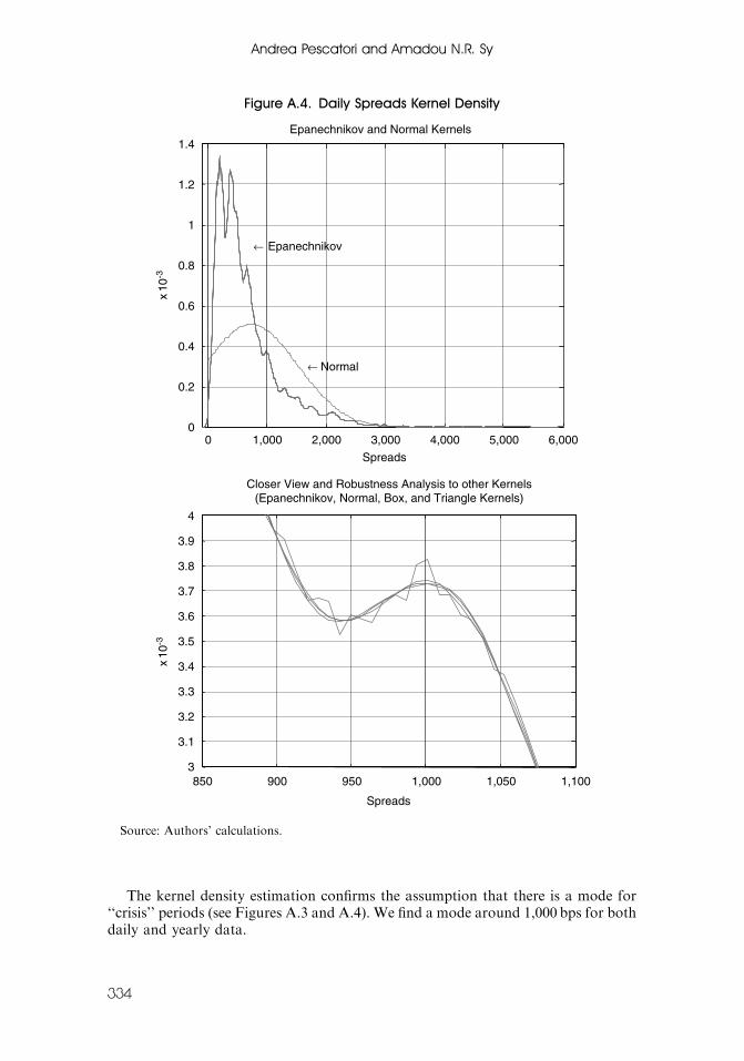
The kernel density estimation confirms the assumption that there is a mode for‘‘crisis’’ periods (see Figures A.3 and A.4). We find a mode around 1,000 bps for bothdaily and yearly data.

Figure A.4. Daily Spreads Kernel Density

Epanechnikov and Normal Kernels

0 1,000 2,000 3,000 4,000 5,000 6,0000

0.2

0.4

0.6

0.8

1

1.2

1.4

x 10

-3x

10-3

Spreads

Epanechnikov

Normal

Closer View and Robustness Analysis to other Kernels (Epanechnikov, Normal, Box, and Triangle Kernels)

850 900 950 1,000 1,050 1,1003

3.1

3.2

3.3

3.4

3.5

3.6

3.7

3.8

3.9

4

Spreads→

→



334

REFERENCESAlesina, Alberto, Alessandro Prati, and Guido Tabellini, 1990, ‘‘Public Confidence andDebt Management: A Model and a Case Study of Italy,’’ in Public Debt Management:Theory and History, ed. by Rudiger Dornbusch and Mario Draghi (Cambridge,Cambridge University Press).

Altman, Edward I., 1998, ‘‘Market Dynamics and Investment Performance ofDistressed and Defaulted Debt Securities,’’ Working Paper (New York, New YorkUniversity).

Beim, David O., and Charles W. Calomiris, 2001, Emerging Financial Markets (NewYork, McGraw-Hill/Irwin).

Berg, Andrew, and Catherine Pattillo, 1999, ‘‘Are Currency Crises Predictable? A Test,’’Staff Papers, International Monetary Fund, Vol. 46 (June), pp. 107–138.

Bussiere, Matthieu, and Christian Mulder, 1999, ‘‘External Vulnerability in EmergingMarket Economies: How High Liquidity Can Offset Weak Fundamentals and theEffects of Contagion,’’ IMF Working Paper 99/88 (Washington, InternationalMonetary Fund).

Calvo, Guillermo A., 1988, ‘‘Servicing the Public Debt: The Role of Expectations,’’American Economic Review, Vol. 78 (September), pp. 647–661.

Chambers, John, and Daria Alexeeva, 2003, ‘‘2002 Defaults and Rating Transition DataUpdate for Rated Sovereigns,’’ in Ratings Performance 2002, Default, Transition,Recovery, and Spreads (New York, Standard & Poor’s), pp. 75–86. Available via theInternet: http://www.standardandpoors.co.jp/spf/pdf/products/RatingsPerformance.pdf.

Chan-Lau, Jorge, 2003, ‘‘Anticipating Credit Events Using Credit Default Swaps, with anApplication to Sovereign Debt Crises,’’ IMF Working Paper 03/106 (Washington,International Monetary Fund).

Dailami, Mansoor, Paul R. Masson, and Jean Jose Padou, 2005, ‘‘Global MonetaryConditions vs. Country-Specific Factors in the Determination of Emerging MarketDebt Spreads,’’ Policy Research Working Paper No. 3626 (Washington, WorldBank).

Detragiache, Enrica, and Antonio Spilimbergo, 2001, ‘‘Crises and Liquidity: Evidenceand Interpretation,’’ IMF Working Paper 01/2 (Washington, International MonetaryFund).

Duffie, Darrell, and Kenneth J. Singleton, 2003, Credit Risk: Pricing, Measurement, andManagement (Princeton, New Jersey, Princeton University Press).

Edwards, Sebastian, 1984, ‘‘LDC Foreign Borrowing and Default Risk: An EmpiricalInvestigation, 1976–80,’’ American Economic Review, Vol. 74 (September), pp. 726–734.

Eichengreen, Barry, and Ashoka Mody, 1998, ‘‘What Explains Changing Spreads onEmerging-Market Debt: Fundamentals or Market Sentiment?’’ NBER WorkingPaper No. 6408 (Cambridge, Massachusetts, National Bureau of EconomicResearch).

———, 1999, ‘‘Lending Booms, Reserves, and the Sustainability of Short-TermDebt: Inferences from the Pricing of Syndicated Bank Loans,’’ NBER WorkingPaper No. 7113 (Cambridge, Massachusetts, National Bureau of EconomicResearch).

Frankel, Jeffrey A., and Andrew K. Rose, 1996, ‘‘Currency Crashes in EmergingMarkets: An Empirical Treatment,’’ Journal of International Economics, Vol. 41(November), pp. 351–366.


335

Garcia, Marcio, and Roberto Rigobon, 2004, ‘‘A Risk Management Approach toEmerging Market’s Sovereign Debt Sustainability with an Application to BrazilianData,’’ NBER Working Paper No. 10336 (Cambridge, Massachusetts, NationalBureau of Economic Research).

Hols, M.C.A.B., and C.G. de Vries, 1991, ‘‘The Limiting Distribution of ExtremalExchange Rate Returns,’’ Journal of Applied Econometrics, Vol. 6 (June–September),pp. 287–302.

Hu, Yen-Ting, Rudiger Kiesel, and William Perraudin, 2001, ‘‘The Estimation ofTransition Matrices for Sovereign Credit Ratings,’’ (unpublished; London, Bank ofEngland). Available via the Internet: http://www3.imperial.ac.uk/portal/pls/portallive/docs/1/43673.PDF.

Juttner, Johannes D., and Justin McCarthy, 1998, ‘‘Modelling a Ratings Crisis,’’(unpublished; Sydney, Australia, Macquarie University).

Kaminsky, Graciela, and Sergio Schumkler, 2001, ‘‘Emerging Markets Instability: DoSovereign Ratings Affect Country Risk and Stock Returns?’’ Policy ResearchWorking Paper No. 2678 (Washington, World Bank).

Koedijk, K.G., M.M.A. Schafgans, and C.G. de Vries, 1990, ‘‘The Tail Index ofExchange Rate Returns,’’ Journal of International Economics, Vol. 29 (August), pp.93–108.

Koedijk, K.G., P.A. Stork, and C.G. de Vries, 1992, ‘‘Differences Between ForeignExchange Rate Regimes: The View from the Tails,’’ Journal of International Moneyand Finance, Vol. 11 (October), pp. 462–473.

Manasse, Paolo, Nouriel Roubini, and Axel Schimmelpfennig, 2003, ‘‘PredictingSoveregin Debt Crises,’’ IMF Working Paper 03/221 (Washington: InternationalMonetary Fund).

Mauro, Paolo, Nathan Sussman, and Yishay Yafeh, 2002, ‘‘Emerging Market Spreads:Then vs. Now,’’ Quarterly Journal of Economics, Vol. 117 (May), pp. 695–733.

McDonald, D., 1982, ‘‘Debt Capacity and Developing Country Borrowing: A Surveyof the Literature,’’ Staff Papers, International Monetary Fund, Vol. 29, pp.603–646.

Milesi-Ferretti, Gian Maria, and Assaf Razin, 1998, ‘‘Current Account Reversals andCurrency Crises: Empirical Regularities,’’ IMF Working Paper 98/89 (Washington,International Monetary Fund).

Moody’s Investors Service, 2003, ‘‘Sovereign Bond Defaults, Rating Transitions, andRecoveries (1985–2002)’’ Special comments (February), pp. 2–52.

Pozo, Susan, and Catalina Amuedo-Dorantes, 2003, ‘‘Statistical Distributions and theIdentification of Currency Crises,’’ Journal of International Money and Finance, Vol.22 (August), pp. 591–609.

Radelet, Steven, and Jeffrey Sachs, 1998, ‘‘The East Asian Financial Crisis: Diagnosis,Remedies, Prospects,’’ Brookings Papers on Economic Activity: 1 (BrookingsInstitution), pp. 1–90 (Washington D.C., Brookings Institution).

Reinhart, Carmen M., 2002, ‘‘Default, Currency Crises and Sovereign Credit Ratings,’’NBER Working Paper No. 8738 (Cambridge, Massachusetts, National Bureau ofEconomic Research). Also in World Bank Economic Review, Vol. 16, No. 2, pp.151–70.

Rodrik, Dani, and Andres Velasco, 2000, ‘‘Short-Term Capital Flows,’’ in Proceedings ofthe 1999 Annual Bank Conference on Development Economics, ed. by Boris Pleskovicand Joseph E. Stiglitz (Washington, World Bank).


336

Sachs, Jeffrey D., 1984, Theoretical Issues in International Borrowing, Princeton Studies inInternational Finance No. 54 (Princeton, New Jersey, Princeton University Press).

Standard and Poor’s, 2002, ‘‘Sovereign Defaults: Moving Higher Again in 2003?’’September 24, 2002. Reprinted for Ratings Direct.

Sy, Amadou N.R, 2004, ‘‘Rating the Rating Agencies: Anticipating Currency Crises orDebt Crises?,’’ Journal of Banking and Finance, Vol. 28 (November), pp. 2845–2867.


337

IMF Staff Papers, Vol. 54, No. 2, 2007: Are Debt Crises Adequately ...

Documents

Transcript of IMF Staff Papers, Vol. 54, No. 2, 2007: Are Debt Crises Adequately ...