IMC Filter Design for PID Controller Tuning of Time ... · processes with large process time...
36
12 IMC Filter Design for PID Controller Tuning of Time Delayed Processes M. Shamsuzzoha 1 and Moonyong Lee 2 1 Department of Chemical Engineering, King Fahd University of Petroleum and Minerals, Daharan, 2 School of Chemical Engineering, Yeungnam University, Kyongsa, 1 Kingdom of Saudi Arabia 2 Korea 1. Introduction The proportional integral derivative (PID) control algorithm is widely used in process industries because of its simplicity, robustness and successful practical application. Although advanced control techniques can show significantly improved performance, a PID control system can suffice for many industrial control loops. A survey by Desborough and Miller (2002) of over 11,000 controllers in the process industries found that over 97% of regulatory controllers use the PID algorithm. Kano and Ogawa (2010) reported that PID control, conventional advanced control and model predictive control are used in an approximately 100:10:1 ratio. Although, a PID controller has only three adjustable parameters, finding appropriate settings is not simple, resulting in many controllers being poorly tuned and time consuming plant tests often being necessary to obtain process parameters for improved controller settings. There are several approaches for controller tuning, with that based on an open-loop model (g) being most popular. This model is typically given in terms of the plant’s gain (K), time constant (τ) and time delay (θ). For a given a plant model, g, controller settings are often obtained by direct synthesis (Seborg et al., 2004). The IMC-PID tuning method of Rivera et al. (1986) is also popular. Original direct synthesis approaches, like that of Rivera et al. (1986), give very good performance for set-point changes, but show slow responses to input (load) disturbances for lag-dominant (including integrating) processes with θ/τ < 0.1. To improve load disturbance rejection, Shamsuzzoha and Lee (2007a and b, 2008a and b) proposed modified IMC-PID tuning methods for different types of process. For PI tuning, Skogestad (2003) proposed a modified SIMC method where the integral time is reduced for processes with large process time constants, τ. PI/PID tuning based on the IMC and direct synthesis approaches has only one tuning parameter: the closed-loop time constant, τ c . Tuning approaches based on an open-loop plant require an open-loop model (g) of the process to be obtained first. This generally involves an initial open-loop experiment, for example a step test, to acquire the required process data. This can be time consuming and www.intechopen.com
Transcript of IMC Filter Design for PID Controller Tuning of Time ... · processes with large process time...

12
IMC Filter Design for PID Controller Tuning of Time Delayed Processes
M. Shamsuzzoha1 and Moonyong Lee2
1Department of Chemical Engineering, King Fahd University of Petroleum and Minerals, Daharan,
2School of Chemical Engineering, Yeungnam University, Kyongsa, 1Kingdom of Saudi Arabia
2Korea
1. Introduction
The proportional integral derivative (PID) control algorithm is widely used in process industries because of its simplicity, robustness and successful practical application. Although advanced control techniques can show significantly improved performance, a PID control system can suffice for many industrial control loops.
A survey by Desborough and Miller (2002) of over 11,000 controllers in the process industries found that over 97% of regulatory controllers use the PID algorithm. Kano and Ogawa (2010) reported that PID control, conventional advanced control and model predictive control are used in an approximately 100:10:1 ratio. Although, a PID controller has only three adjustable parameters, finding appropriate settings is not simple, resulting in many controllers being poorly tuned and time consuming plant tests often being necessary to obtain process parameters for improved controller settings.
There are several approaches for controller tuning, with that based on an open-loop model (g) being most popular. This model is typically given in terms of the plant’s gain (K), time constant (τ) and time delay (θ). For a given a plant model, g, controller settings are often obtained by direct synthesis (Seborg et al., 2004). The IMC-PID tuning method of Rivera et al. (1986) is also popular. Original direct synthesis approaches, like that of Rivera et al. (1986), give very good performance for set-point changes, but show slow responses to input (load) disturbances for lag-dominant (including integrating) processes with θ/τ < 0.1. To improve load disturbance rejection, Shamsuzzoha and Lee (2007a and b, 2008a and b) proposed modified IMC-PID tuning methods for different types of process. For PI tuning, Skogestad (2003) proposed a modified SIMC method where the integral time is reduced for processes with large process time constants, τ. PI/PID tuning based on the IMC and direct synthesis approaches has only one tuning parameter: the closed-loop time constant, τc.
Tuning approaches based on an open-loop plant require an open-loop model (g) of the process to be obtained first. This generally involves an initial open-loop experiment, for example a step test, to acquire the required process data. This can be time consuming and
www.intechopen.com
PID Controller Design Approaches – Theory, Tuning and Application to Frontier Areas
254
may result in undesirable output changes. Approximations can then be used to obtain the process model, g, from the open-loop data.
A two-step procedure, based on a closed-loop set-point experiment with a P-controller, was originally proposed by Yuwana and Seborg (1982). They developed a first-order with delay model by matching the closed-loop set-point response with a standard oscillating second-order step response that results when the time delay is approximated by a first-order Pade approximation. From the set-point response, they identified the first overshoot, the first undershoot and the second overshoot and then used the Ziegler-Nichols (1942) tuning rules for the final PID controller settings, which shows aggressive responses.
Controller tuning based on closed-loop experiments was initially proposed by Ziegler-Nichols (1942). It can simply and directly obtain controller setting from closed-loop data, without explicitly obtaining an open-loop model, g. This approach requires very little information about the process; namely, the ultimate controller gain (Ku) and the oscillations' period (Pu), which can be obtained from a single experiment. The recommended settings for a PI-controller are Kc=0.45Ku and τI=0.83Pu. However, there are several disadvantages; the system needs to be brought to its limit of instability, which may require many trials. This problem can be circumvented by inducing sustained oscillations with an on-off controller using the relay method of Åström and Hägglund (1984), though this requires the system to have installed the ability to switch to on/off-control. Ziegler-Nichols (1942) tuning does not work well with all processes. Its recommended settings are aggressive for lag-dominant (integrating) processes (Tyreus and Luyben, 1992) and slow for delay-dominant process (Skogestad, 2003). To improve robustness for lag-dominant (integrating) processes, Tyreus and Luyben (1992) proposed the use of less aggressive settings (Kc=0.313Ku and τI=2.2Pu), though this further slowed responses for delay-dominant processes (Skogestad, 2003). This is a fundamental problem of the Ziegler-Nichols (1942) method because it considers only two pieces of information about the process (Ku, Pu), which correspond to the critical point on the Nyquist curve. Therefore, distinguishing between, for example, a lag-dominant and a delay-dominant process is not possible. Additional closed-loop experiments may fix this problem, for example an experiment with an integrating controller (Schei, 1992). A third disadvantage of the Ziegler-Nichols (1942) method is that it can only be used with processes for which the phase lag exceeds -180 degrees at high frequencies. For example, it is inapplicable to a simple second-order process.
Shamsuzzoha and Skogestad (2010) proposed a simple tuning method for a PI/PID controller of an unidentified process using closed-loop experiments. It requires one closed-loop step set-point response experiment using a proportional only controller, and mainly uses information about the first peak (overshoot), which is easily identified. The set-point experiment is similar to that of Ziegler-Nichols (1942) but the controller gain is typically about one half, so the system is not at the stability limit with sustained oscillations. Simulations of a range of first-order with delay processes allow simple correlations to be derived to give PI controller settings similar to those of the SIMC tuning rules (Skogestad, 2003). The recommended controller gain change is a function of the height of the first peak (overshoot); the controller integral time is mainly a function of the time to reach the peak. The method includes a detuning factor that allows the user to adjust the final closed-loop response time and robustness. The proposed tuning method, originally derived for first-order with delay processes, has been tested with a range of other typical processes for
www.intechopen.com
IMC Filter Design for PID Controller Tuning of Time Delayed Processes
255
process control applications and the results are comparable with SIMC tunings using the open-loop model.
The IMC-PID tuning rules have the advantage of using only a single tuning parameter to achieve a clear trade-off between closed-loop performance and robustness against model inaccuracies. The IMC-PID controller provides good set-point tracking but shows slow responses to disturbances, especially for processes with small time-delay/time-constant ratios (Chen and Seborg, 2002; Horn et al., 1996; Shamsuzzoha and Lee, 2007 and 2008; Shamsuzzoha and Skogestad, 2010; Morari and Zafiriou, 1989; Lee et al., 1998; Chien and Fruehauf, 1990; Skogestad, 2003). However, as disturbance rejection is often more important than set-point tracking, designing a controller with improved disturbance rejection rather than set-point tracking is an important problem that much current research aims to address.
The IMC-PID tuning methods of Rivera et al. (1986), Morari and Zafiriou (1989), Horn et al. (1996), Lee et al. (1998) and Lee et al. (2000), and the direct synthesis method of Smith et al. (1975) (DS) and Chen and Seborg (2002) (DS-d) are examples of two typical tuning methods based on achieving a desired closed-loop response. These methods obtain the PID controller parameters by computing the controller which gives the desired closed-loop response. Although this controller is often more complicated than a PID controller, its form can be reduced to that of either a PID controller or a PID controller cascaded with a first- or second-order lag by some clever approximations of the dead time in the process model.
Regarding disturbance rejection for lag time-dominant processes, Ziegler and Nichols' (1942) established design method (ZN) shows better performance than IMC-PID design methods based on the IMC filter f=1/(酵cs+1)r. Horn et al. (1996) proposed a new type of IMC filter that includes a lead term to cancel process-dominant poles. Based on this filter, they developed an IMC-PID tuning rule that leads to the structure of a PID controller with a second-order lead-lag filter. The resulting controller showed advantages over those based on the conventional IMC filter. Chen and Seborg (2002) proposed a direct synthesis design method to improve disturbance rejection in several popular process models. To avoid excessive overshoot in the set-point response, they employed a set-point weighting factor. To improve set-point performance with a set-point filter, Lee et al. (1998) proposed an IMC-PID controller based on both the filter suggested by Horn et al. (1996) and a two-degrees-of-freedom (2DOF) control structure. Lee et al. (2000) extended the tuning method to unstable processes such as first- and second-order delayed unstable process (FODUP and SODUP) models and for set-point performance, they used a 2DOF control structure.
Veronesi and Visioli (2010) reported another two-step approach that assesses and possibly retunes a given PI controller. From a closed-loop set-point or disturbance response of the existing PI controller, a first-order with delay model and time constant are identified and used to assess the closed-loop performance. If performance is worse than expected, the controller is retuned using, for example, the SIMC method. This method has only been developed for integrating processes. Seki and Shigemasa (2010) proposed a controller retuning method based on comparing closed-loop responses obtained with two different controller settings.
The IMC-PID approach determines the performance of the PID controller mainly through the IMC filter structure. Most previous reports of IMC-PID design have the IMC filter
www.intechopen.com

PID Controller Design Approaches – Theory, Tuning and Application to Frontier Areas
256
structure designed as simple as possible while satisfying the necessary performance requirements of the IMC controller. For example, the order of the lead term in the IMC filter is designed small enough to cancel out the dominant process poles and the lag term is set simply to make the IMC controller realizable. However, the performance of the resulting PID controller is determined both by the performance of the IMC controller performance and by how closely the PID controller approximates the ideal controller equivalent to the IMC controller, which mainly depends on the structure of the IMC filter. Therefore, in IMC-PID design, the optimum IMC filter structure has to be selected considering the performance of the resulting PID controller rather than that of the IMC controller.
2. The IMC-PID approach for PID controller design
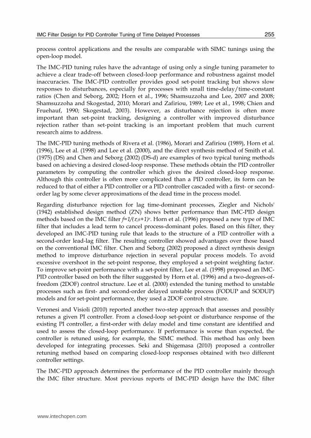
The block diagram of IMC control (Figure 1-a) has pG represent the process, pG the process model, and q the IMC controller. In the IMC control structure, the controlled variable is given by:
1
1 1p p
R dp p p p
G q G qC f R G d
q G G q G G
(1)
In the nominal case of, p pG G the set-point and disturbance responses are simplified to:
p RC
G qfR (2)
1 p dC
G q Gd
(3)
In the classical feedback control structure (Figure (1-b)), the set-point and disturbance responses are respectively:
1
c p R
c p
G G fC
R G G (4)
1
d
c p
GC
d G G (5)
where cG denotes the equivalent feedback controller.
IMC parameterization (Morari and Zafiriou, 1989) allows the process model pG to be decomposed into two parts:
p M AG P P (6)
www.intechopen.com
IMC Filter Design for PID Controller Tuning of Time Delayed Processes
257
where MP and AP are the portions of the model that are inverted and not inverted, respectively, by the controller ( AP is usually a non-minimum phase and contains dead times and/or right half plane zeros); 0 1AP .
(a) The IMC structure
(b) Classical feedback control structure
Fig. 1. Block diagrams of IMC and classical feedback control structures
The IMC controller is designed by:
-1Mq P f (7)
The ideal feedback controller that is equivalent to the IMC controller can be expressed in terms of the internal model, pG , and the IMC controller, q :
1c
p
qG
G q (8)
Since the resulting controller does not have the form of a standard PID controller, it remains to design the PID controller to approximate the equivalent feedback controller most closely. Lee et al. (1998) proposed an efficient method for converting the ideal feedback controller,
cG , to a standard PID controller. Since cG has an integral term, it can be expressed as:
www.intechopen.com

PID Controller Design Approaches – Theory, Tuning and Application to Frontier Areas
258
c
g sG
s (9)
Expanding cG in Maclaurin series in s gives:
''' 201
0 0 ...2c
gG g g s s
s
(10)
The first three terms of which can be interpreted as the standard PID controller which is given by:
1
1c c DI
G K ss
(11)
where
' 0cK g (12a)
' 0 0I g g (12b)
'' '0 2 0D g g (12c)
3. IMC-PID tuning rules for typical process models
This section proposes tuning rules for several typical time-delayed processes.
3.1 First-Order Plus Dead time Process (FOPDT)
The most commonly used approximate model for chemical processes is the FOPDT model:
1
s
p dKe
G Gs
(13)
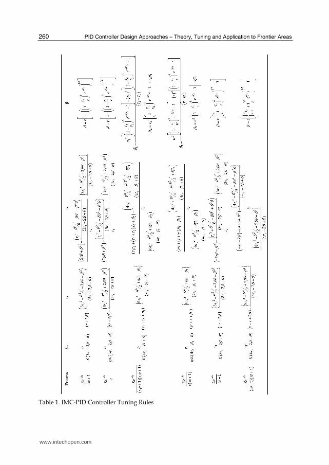
where K is the gain, τ the time constant and θ the time delay. The optimum IMC filter structure is 321 1cf s s and the resulting IMC controller becomes 321 1 1cq s s K s . Therefore the ideal feedback controller, which is equivalent to the IMC controller, is:
2
3 2
1 1
1 1c
sc
s sG
K s e s
(14)
The analytical PID formula can be obtained from Eq. (12) as:
www.intechopen.com

IMC Filter Design for PID Controller Tuning of Time Delayed Processes
259
3 2I
cc
KK
(15a)
22 23 22
23 2
c
Ic
(15b)
33 2 2
22 2 26
2 3 23 2 23 2
c
cc
DI c
(15c)
The value of the extra degree of freedom, β, is selected so that it cancels the open-loop pole at 1s that slows responses to load disturbance. Thus, β is chosen so that the term
1 Gq has a zero at the pole of dG , so that 11 0
sGq and
32
11 1 1 0s
cs
s e s
. After simplification, β becomes:
1 23
1 1 c e (16)
3.2 Delayed Integrating Process (DIP)
s
p dKe
G Gs
(17)
A delayed integrating process (DIP) can be modeled by considering the integrator as a stable pole near zero because the above IMC procedure is not applicable to DIPs, since the β term disappears at 0s . A controller based on a model with a stable pole near zero can give more robust closed-loop responses than one based on a model with an integrator or unstable pole near zero, as suggested by Lee et al. (2000). Therefore, a DIP can be approximated to a FOPDT as follows:
1 / 1
s s s
p dKe Ke Ke
G Gs s s
(18)
where Ψ is a sufficiently large arbitrary constant. Accordingly, the optimum filter structure
for a DIP is same as that for a FOPDT, i.e. 321 1cf s s .
Therefore, the resulting IMC controller becomes 321 1 1cq s s K s and the
ideal feedback controller is
2
3 2
1 1
1 1c
sc
s sG
K s e s
. The resulting PID tuning
rules are listed in Table 1.
www.intechopen.com
PID Controller Design Approaches – Theory, Tuning and Application to Frontier Areas
260
Table 1. IMC-PID Controller Tuning Rules
www.intechopen.com
IMC Filter Design for PID Controller Tuning of Time Delayed Processes
261
3.3 Second-Order Plus Dead time Process (SOPDT)
Consider a stable SOPDT system:
1 21 1
s
p dKe
G Gs s
(19)
The optimum IMC filter structure is 422 1 1 1cf s s s . The IMC controller
becomes 421 2 2 11 1 1 1cq s s s s K s and the ideal feedback controller
equivalent to the IMC controller is
21 2 2 1
4 22 1
1 1 1
1 1c
sc
s s s sG
K s e s s
. The resulting
PID tuning rules are listed in Table 1.
3.4 First-Order Delayed Integrating Process (FODIP)
Consider the following FODIP system:
1
s
p dKe
G Gs s
(20)
It can be approximated as the SOPDT model, becoming:
1 1 1
s s
p dKe Ke
G Gs s s s
(21)
where Ψ is a sufficiently large arbitrary constant. Thus, the optimum IMC filter is same as
that for the SOPDT, 422 1 1 1cf s s s and the resulting IMC controller
becomes 422 11 1 1 1cq s s s s K s . The resulting PID tuning rules are
listed in Table 1.
3.5 First-Order Delayed Unstable Process (FODUP)
One of the most commonly considered unstable processes with time delay is the FODUP:
1
s
p dKe
G Gs
(22)
The optimum IMC filter is 321 1cf s s . Therefore, the IMC controller becomes
321 1 1cq s s K s and the ideal feedback controller is
2
3 2
1 1
1 1c
sc
s sG
K s e s
. The resulting PID tuning rules are listed in Table 1.
www.intechopen.com

PID Controller Design Approaches – Theory, Tuning and Application to Frontier Areas
262
3.6 Second-Order Delayed Unstable Process (SODUP)
The process model is:
1 1
s
p dKe
G Gs as
(23)
The optimum IMC filter is 421 1cf s s and the IMC controller
is 421 1 1 1cq s as s K s . The resulting PID tuning rules are listed in Table
1.
4. Performance and robustness evaluation
The performance and robustness of a control system are evaluated by the following indices.
4.1 Integral error criteria
Three commonly used performance indices based on integral error can evaluate performance: the integral of the absolute error (IAE), the integral of the squared error (ISE), and the integral of the time-weighted absolute error (ITAE).
0
IAE e t dt (24)
20
ISE e t dt (25)
0
ITAE t e t dt (26)
where the error signal e t is the difference between the set-point and the measurement.
The ISE criterion penalizes larger errors; the ITAE criterion, long-term errors. The IAE criterion tends to produce controller settings that are between those of the ITAE and ISE criteria.
4.2 Overshoot
Overshoot is a measure of by how much the response exceeds the ultimate value following a step change in set-point and/or disturbance.
4.3 Maximum sensitivity (Ms) to modeling error
A control system's maximum sensitivity, max 1 /[1 ( )]s p cM G G i , can be used to
evaluate its robustness. Since Ms is the inverse of the shortest distance from the Nyquist
www.intechopen.com
IMC Filter Design for PID Controller Tuning of Time Delayed Processes
263
curve of the loop transfer function to the critical point (-1, 0), a low Ms indicates that the control system has a large stability margin. Ms is typically between 1.2 and 2.0 (Åström et al., 1998). To ensure a fair comparison, all the controller simulation examples considered here are designed to have the same robustness level in terms of maximum sensitivity.
4.4 Total Variation (TV)
To evaluate the manipulated input usage the TV of the input u(t) is computed as the sum of all its moves up and down. Considering the the input signal as a discrete sequence
1 2 3[ , , ...., ...],iu u u u leads to 11
i ii
TV u u
, which should be minimized. TV is a good
measure of a signal's smoothness (Skogestad, 2003).
4.5 Set-point and derivative weighting
The conventional form of the PID controller used here for simulation is:
1
1PID c DI
G K ss
(27)
A more widely accepted control structure that includes set-point weighting and derivative weighting is given by Åström and Hägglund (1995):
0
1 t
c DI
d cr t y tu t K br t y t r t y t d
dt
(28)
where b and c are additional parameters. The integral term must be based on error feedback to ensure the desired steady state. The controller structure in Eq. (28) has two degrees of freedom. The set-point weighting coefficient b is bounded by 0 1b and the derivative weighting coefficient c is bounded by 0 1c . The overshoot for set-point changes decreases with decreasing b.
The controllers obtained with different values of b and c respond to disturbances and measurement noise in the same way as a conventional PID controller, i.e. the values of b and c do not affect the closed-loop responses to disturbances (Chen and Seborg, 2002). Therefore, the PID tuning rules developed here are also applicable for the modified PID controller in Eq. (28). However, the set-point response does depend on the values of b and c. Throughout this study,
c=1, while the set-point filter 21 1R I I D If b s s s was used with 0 1b .
5. Simulation results
Six process models are simulated here. They are common processes widely used in the chemical industry and have been studied by other researchers. In each case, different performance and robustness matrices have been calculated and are compared with other existing methods. The method of Shamsuzzoha and Lee (2007a), the SL method for conciseness, is compared with other reported tuning methods.
www.intechopen.com
PID Controller Design Approaches – Theory, Tuning and Application to Frontier Areas
264
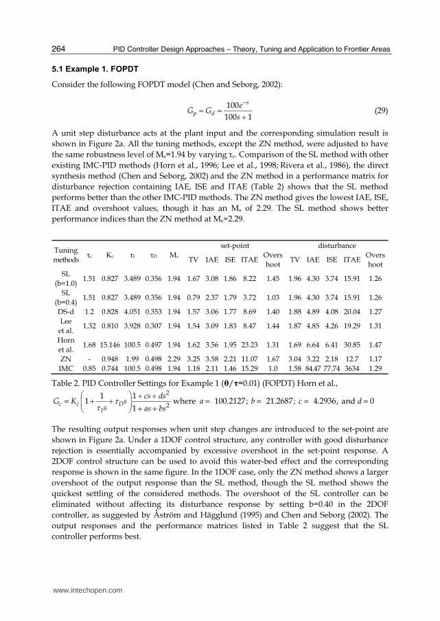
5.1 Example 1. FOPDT
Consider the following FOPDT model (Chen and Seborg, 2002):
100
100 1
s
p de
G Gs
(29)
A unit step disturbance acts at the plant input and the corresponding simulation result is shown in Figure 2a. All the tuning methods, except the ZN method, were adjusted to have the same robustness level of Ms=1.94 by varying τc. Comparison of the SL method with other existing IMC-PID methods (Horn et al., 1996; Lee et al., 1998; Rivera et al., 1986), the direct synthesis method (Chen and Seborg, 2002) and the ZN method in a performance matrix for disturbance rejection containing IAE, ISE and ITAE (Table 2) shows that the SL method performs better than the other IMC-PID methods. The ZN method gives the lowest IAE, ISE, ITAE and overshoot values, though it has an Ms of 2.29. The SL method shows better performance indices than the ZN method at Ms=2.29.
Tuning methods
τc Kc τI τD Ms
set-point disturbance
TV IAE ISE ITAEOvershoot
TV IAE ISE ITAE Overshoot
SL (b=1.0)
1.51 0.827 3.489 0.356 1.94 1.67 3.08 1.86 8.22 1.45 1.96 4.30 3.74 15.91 1.26
SL (b=0.4)
1.51 0.827 3.489 0.356 1.94 0.79 2.37 1.79 3.72 1.03 1.96 4.30 3.74 15.91 1.26
DS-d 1.2 0.828 4.051 0.353 1.94 1.57 3.06 1.77 8.69 1.40 1.88 4.89 4.08 20.04 1.27 Lee
et al. 1.32 0.810 3.928 0.307 1.94 1.54 3.09 1.83 8.47 1.44 1.87 4.85 4.26 19.29 1.31
Horn et al.
1.68 15.146 100.5 0.497 1.94 1.62 3.56 1.95 23.23 1.31 1.69 6.64 6.41 30.85 1.47
ZN - 0.948 1.99 0.498 2.29 3.25 3.58 2.21 11.07 1.67 3.04 3.22 2.18 12.7 1.17 IMC 0.85 0.744 100.5 0.498 1.94 1.18 2.11 1.46 15.29 1.0 1.58 84.47 77.74 3634 1.29
Table 2. PID Controller Settings for Example 1 (曽/訴=0.01) (FOPDT) Horn et al., 2
21 1
11
c c DI
cs dsG K s
s as bs
where 100.2127; 21.2687; 4.2936, and 0a b c d
The resulting output responses when unit step changes are introduced to the set-point are shown in Figure 2a. Under a 1DOF control structure, any controller with good disturbance rejection is essentially accompanied by excessive overshoot in the set-point response. A 2DOF control structure can be used to avoid this water-bed effect and the corresponding response is shown in the same figure. In the 1DOF case, only the ZN method shows a larger overshoot of the output response than the SL method, though the SL method shows the quickest settling of the considered methods. The overshoot of the SL controller can be eliminated without affecting its disturbance response by setting b=0.40 in the 2DOF controller, as suggested by Åström and Hägglund (1995) and Chen and Seborg (2002). The output responses and the performance matrices listed in Table 2 suggest that the SL controller performs best.
www.intechopen.com

IMC Filter Design for PID Controller Tuning of Time Delayed Processes
265
The controllers' robustness is evaluated by simultaneously inserting a perturbation uncertainty of 20% in all three parameters to obtain the worst case model mismatch, i.e.
1.2120 80 1p dsG G e s as an actual process. The simulation results for both set-point
and disturbance rejection are listed Table 3. The methods of SL and Chen & Seborg (2002)
(DS-d) give similar error integral values for disturbance rejection. In terms of servo response, the IMC has clear advantages and the methods of Shams & Lee, DS-d, Lee et al. (1998) and Horn et al. (1996) show almost similar robustness.
0 2 4 6 8 10 12 14 160
0.4
0.8
1.2
1.6
2
Time
Pro
cess
Var
iabl
e
0 2 4 6 8 10 12 14 16-0.5
0
0.5
1
1.5
Time
Pro
cess
Var
iabl
e
SL (b=1) Lee et al. (1998) DS-d Horn et al. ZN SL (b=0.4)
SL Lee et al. (1998) DS-d Horn et al. ZN IMC
b
a
Fig. 2. Responses of the nominal system in Example 1.
5.2 Example 2. DIP (Distillation Column Model)
Consider next the distillation column model studied by Chien and Fruehauf (1990) and Chen & Seborg (2002) (DS-d). The column separates a small amount of low-boiling material from the final product. Its bottom level is controlled by adjusting the steam flow rate. The process model for the level control system is represented as the following DIP model, which can be approximated by the FOPDT model for design of the PID controller:
7.4 7.40.2 20
100 1
s s
p de e
G Gs s
(30)
www.intechopen.com
PID Controller Design Approaches – Theory, Tuning and Application to Frontier Areas
266
Tuning methods set-point disturbance
TV IAE ISE ITAE Over shoot
TV IAE ISE ITAE Over shoot
SL (b=1.0) 6.36 5.47 3.50 27.77 2.12 7.33 6.31 6.39 36.03 1.95
DS-d 6.20 5.23 3.24 26.46 2.06 7.19 6.28 6.50 35.53 1.96 Lee et al. 5.93 5.61 3.49 30.0 2.09 7.00 6.80 7.07 40.39 2.1
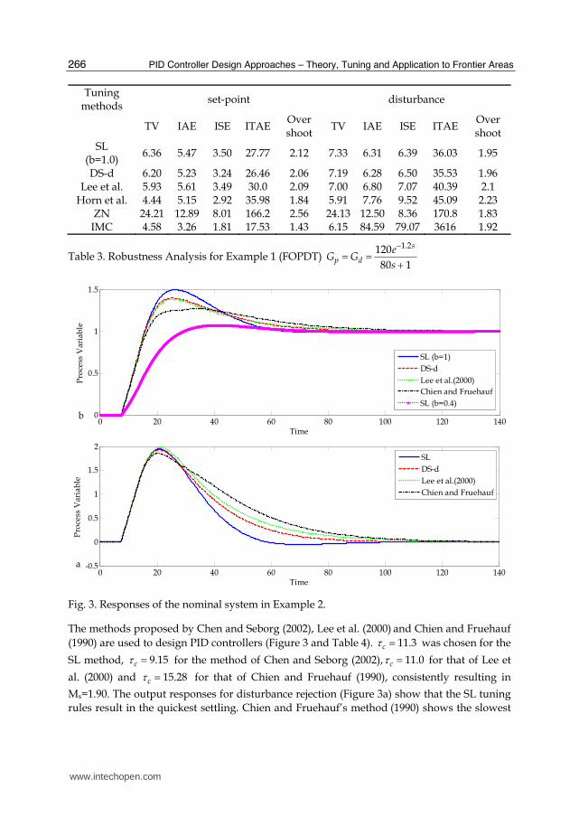
Horn et al. 4.44 5.15 2.92 35.98 1.84 5.91 7.76 9.52 45.09 2.23 ZN 24.21 12.89 8.01 166.2 2.56 24.13 12.50 8.36 170.8 1.83 IMC 4.58 3.26 1.81 17.53 1.43 6.15 84.59 79.07 3616 1.92
Table 3. Robustness Analysis for Example 1 (FOPDT) 1.2120
80 1
s
p de
G Gs
0 20 40 60 80 100 120 1400
0.5
1
1.5
Time
Pro
cess
Var
iabl
e
0 20 40 60 80 100 120 140-0.5
0
0.5
1
1.5
2
Time
Pro
cess
Var
iabl
e
SLDS-dLee et al.(2000)Chien and Fruehauf
SL (b=1)DS-dLee et al.(2000)Chien and FruehaufSL (b=0.4)
a
b
Fig. 3. Responses of the nominal system in Example 2.
The methods proposed by Chen and Seborg (2002), Lee et al. (2000) and Chien and Fruehauf
(1990) are used to design PID controllers (Figure 3 and Table 4). 11.3c was chosen for the
SL method, 9.15c for the method of Chen and Seborg (2002), 11.0c for that of Lee et
al. (2000) and 15.28c for that of Chien and Fruehauf (1990), consistently resulting in Ms=1.90. The output responses for disturbance rejection (Figure 3a) show that the SL tuning rules result in the quickest settling. Chien and Fruehauf’s method (1990) shows the slowest
www.intechopen.com
IMC Filter Design for PID Controller Tuning of Time Delayed Processes
267
response and the longest settling time. The performance matrix (Table 4) shows that the SL method gives the lowest error integral value, while Chien and Fruehauf’s (1990) method gives the highest at the same robustness level.
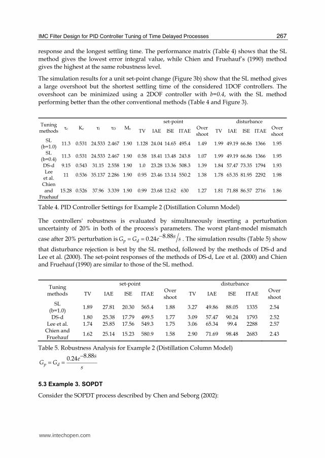
The simulation results for a unit set-point change (Figure 3b) show that the SL method gives a large overshoot but the shortest settling time of the considered 1DOF controllers. The overshoot can be minimized using a 2DOF controller with b=0.4, with the SL method performing better than the other conventional methods (Table 4 and Figure 3).
Tuning methods
τc Kc τI τD Ms
set-point disturbance
TV IAE ISE ITAEOver shoot
TV IAE ISE ITAE Over shoot
SL (b=1.0) 11.3 0.531 24.533 2.467 1.90 1.128 24.04 14.65 495.4 1.49 1.99 49.19 66.86 1366 1.95
SL (b=0.4)
11.3 0.531 24.533 2.467 1.90 0.58 18.41 13.48 243.8 1.07 1.99 49.19 66.86 1366 1.95
DS-d 9.15 0.543 31.15 2.558 1.90 1.0 23.28 13.36 508.3 1.39 1.84 57.47 73.35 1794 1.93 Lee
et al. 11 0.536 35.137 2.286 1.90 0.95 23.46 13.14 550.2 1.38 1.78 65.35 81.95 2292 1.98
Chien and
Fruehauf 15.28 0.526 37.96 3.339 1.90 0.99 23.68 12.62 630 1.27 1.81 71.88 86.57 2716 1.86
Table 4. PID Controller Settings for Example 2 (Distillation Column Model)
The controllers' robustness is evaluated by simultaneously inserting a perturbation uncertainty of 20% in both of the process's parameters. The worst plant-model mismatch
case after 20% perturbation is 8.880.24p dsG G e s . The simulation results (Table 5) show
that disturbance rejection is best by the SL method, followed by the methods of DS-d and Lee et al. (2000). The set-point responses of the methods of DS-d, Lee et al. (2000) and Chien and Fruehauf (1990) are similar to those of the SL method.
Tuning methods
set-point disturbance
TV IAE ISE ITAE Over shoot
TV IAE ISE ITAE Over shoot
SL (b=1.0)
1.89 27.81 20.30 565.4 1.88 3.27 49.86 88.05 1335 2.54
DS-d 1.80 25.38 17.79 499.5 1.77 3.09 57.47 90.24 1793 2.52 Lee et al. 1.74 25.85 17.56 549.3 1.75 3.06 65.34 99.4 2288 2.57
Chien and Fruehauf
1.62 25.14 15.23 580.9 1.58 2.90 71.69 98.48 2683 2.43
Table 5. Robustness Analysis for Example 2 (Distillation Column Model) 8.880.24
p d
seG G
s
5.3 Example 3. SOPDT
Consider the SOPDT process described by Chen and Seborg (2002):
www.intechopen.com
PID Controller Design Approaches – Theory, Tuning and Application to Frontier Areas
268
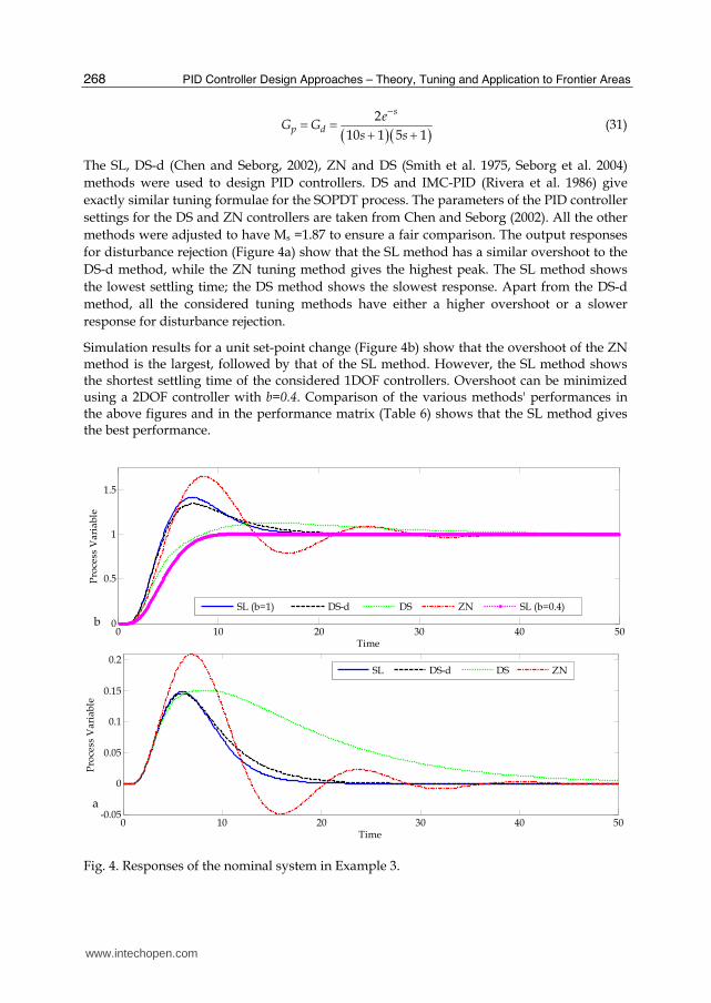
210 1 5 1
s
p de
G Gs s
(31)
The SL, DS-d (Chen and Seborg, 2002), ZN and DS (Smith et al. 1975, Seborg et al. 2004) methods were used to design PID controllers. DS and IMC-PID (Rivera et al. 1986) give exactly similar tuning formulae for the SOPDT process. The parameters of the PID controller settings for the DS and ZN controllers are taken from Chen and Seborg (2002). All the other methods were adjusted to have Ms =1.87 to ensure a fair comparison. The output responses for disturbance rejection (Figure 4a) show that the SL method has a similar overshoot to the DS-d method, while the ZN tuning method gives the highest peak. The SL method shows the lowest settling time; the DS method shows the slowest response. Apart from the DS-d method, all the considered tuning methods have either a higher overshoot or a slower response for disturbance rejection.
Simulation results for a unit set-point change (Figure 4b) show that the overshoot of the ZN method is the largest, followed by that of the SL method. However, the SL method shows the shortest settling time of the considered 1DOF controllers. Overshoot can be minimized using a 2DOF controller with b=0.4. Comparison of the various methods' performances in the above figures and in the performance matrix (Table 6) shows that the SL method gives the best performance.
0 10 20 30 40 500
0.5
1
1.5
Time
Proc
ess
Var
iabl
e
0 10 20 30 40 50-0.05
0
0.05
0.1
0.15
0.2
Time
Proc
ess
Var
iabl
e
SL DS-d DS ZN
SL (b=1) DS-d DS ZN SL (b=0.4)
a
b
Fig. 4. Responses of the nominal system in Example 3.
www.intechopen.com

IMC Filter Design for PID Controller Tuning of Time Delayed Processes
269
The methods' robustness is evaluated by considering the worst plant-model mismatch case
of 1.22.4 8 1 4 1sp dG G e s s by simultaneously inserting a perturbation uncertainty
of 20% in all three parameters (Table 7). Of the considered methods, the error integral values of the SL method are the best for both set-point and disturbance rejection. The overshoot of the SL method is similar to those of the DS-d and DS methods. The ZN method shows the largest overshoot of the considered methods.
Tuning methods
τc Kc τI τD Ms
set-point disturbance
TV IAE ISE ITAEOvershoot
TV IAE ISE ITAE Over shoot
SL (b=1.0)
1.6 6.415 6.859 1.9798 1.87 11.59 5.66 3.36 28.50 1.41 1.83 1.06 0.11 7.90 0.14
SL (b=0.4)
1.6 6.415 6.859 1.9798 1.87 4.86 4.72 3.63 13.17 1.0 1.83 1.06 0.11 7.90 0.14
DS-d 2.4 6.384 7.604 2.0977 1.87 10.82 5.67 3.22 31.19 1.34 1.71 1.19 0.12 9.77 0.14 SIMC 0.43 3.496 5.72 5.0 1.87 5.514 10.08 4.77 133.6 1.36 1.47 2.50 0.26 38.50 0.16
DS 0.5 5.0 15.0 3.33 1.91 7.18 6.53 3.28 68.19 1.12 1.42 3.0 0.31 49.47 0.15 ZN - 4.72 5.83 1.46 2.26 12.75 8.73 4.88 78.02 1.65 2.71 1.79 0.23 18.9 0.21
Table 6. PID Controller Settings for Example 3 (SOPDT)
Tuning methods
set-point disturbance
TV IAE ISE ITAE Over shoot TV IAE ISE ITAE
Over shoot
SL (b=1.0)
41.88 5.11 2.95 29.45 1.46 6.41 1.09 0.11 8.61 0.17
DS-d 47.93 5.14 2.87 33.12 1.38 7.40 1.21 0.19 10.49 0.17 SIMC 50.36 8.71 3.99 104.9 1.37 14.19 2.31 0.25 31.78 0.18
DS 82.83 6.34 2.99 76.93 1.22 16.50 3.00 0.30 49.41 0.17 ZN 14.90 6.00 3.88 30.23 1.68 3.09 1.29 0.22 8.69 0.24
Table 7. Robustness Analysis for Example 3 (SOPDT) 1.22.4
8 1 4 1
s
p de
G Gs s
5.4 Example 4. FODIP (reboiler level model)
Consider the level control problem proposed by Chen and Seborg (2002). It is an approximate model of the liquid level in the reboiler of a steam heated distillation column, which is controlled by adjusting a control valve on the steam line. The process model is given by:
1.6 0.5 13 1p d
sG G
s s
(32)
This kind of “inverse response time constant” (negative numerator time constant) can be
approximated as a time delay such as 1invinvs e
This is reasonable since an inverse response can deteriorate control similar to a time delay (Skogestad, 2003).
www.intechopen.com

PID Controller Design Approaches – Theory, Tuning and Application to Frontier Areas
270
Therefore, the above model can be approximated as:
0.51.6
3 1
s
p de
G Gs s
(33)
This process can be treated as a FODIP for PID controller design and the tuning parameters can be estimated by the analytical rules given in Table 1.
Disturbance rejection is compared by evaluating the output responses of the SL, the DS-d, the IMC and the ZN methods (Figure 5a, Table 8). The PID controller settings for all the other methods were taken from Chen and Seborg (2002). The SL method has τc=0.935, giving Ms=1.94. The SL output response shows the smallest overshoot and fastest settling, followed by the DS-d and IMC methods. The ZN method shows a very aggressive response with significant overshoot and subsequent oscillation that takes a long time to settle. The SL method clearly shows the best performance of the considered tuning rules.
The output responses for a unit set-point change in the reboiler level model (Figure 5b) show that the SL method with a 1DOF structure gives a large overshoot but shows fast settling to its final value. The overshoot can be greatly reduced using a 2DOF controller. The SL method shows superior performance over the other tuning methods for both set-point and disturbance rejection (Figure 5 and Table 8).
0 5 10 15 20 25 30
0
0.5
1
1.5
2
Time
Pro
cess
Var
iabl
e
0 5 10 15 20 25 30-1.5
-1
-0.5
0
0.5
Time
Pro
cess
Var
iabl
e
SL (b=1) DS-d IMC ZN SL (b=0.4)
SL DS-d IMC ZN
b
a
Fig. 5. Responses of the nominal system in Example 4.
www.intechopen.com
IMC Filter Design for PID Controller Tuning of Time Delayed Processes
271
Tuning methods τc Kc τI τD Ms
set-point disturbance
TV IAE ISE ITAE Over shoot
TV IAE ISE ITAE Over shoot
SL (b=1.0)
0.935 -1.456 4.195 1.250 1.94 4.70 3.087 1.90 9.64 1.40 3.43 2.96 1.38 12.11 -0.66
SL (b=0.4) 0.935 -1.456 4.195 1.250 1.94 1.49 2.536 1.96 4.14 1.01 3.43 2.96 1.38 12.11 -0.66
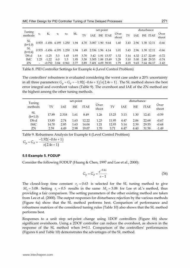
DS-d 1.6 -1.25 5.3 1.45 1.93 3.70 3.42 1.91 13.57 1.32 3.14 4.32 2.17 22.49 -0.72 IMC 1.25 -1.22 6.0 1.5 1.95 3.58 3.505 1.88 15.49 1.28 3.10 5.00 2.48 29.53 -0.74 ZN - -0.752 3.84 0.961 2.77 2.89 7.401 4.09 59.91 1.79 4.03 9.65 7.64 84.17 -1.42
Table 8. PID Controller Settings for Example 4 (Level Control Problem)
The controllers' robustness is evaluated considering the worst case under a 20% uncertainty in all three parameters: 1.92 0.6 1 2.4 1p dG G s s s . The SL method shows the best error integral and overshoot values (Table 9). The overshoot and IAE of the ZN method are the highest among the other tuning methods.
Tuning methods
set-point disturbance
TV IAE ISE ITAE Over shoot
TV IAE ISE ITAE Over shoot
SL (b=1.0) 17.89 2.318 1.61 8.49 1.26 13.23 3.13 1.30 12.41 -0.59
DS-d 13.85 2.74 1.63 12.22 1.23 11.95 4.47 2.06 22.68 -0.67 IMC 14.70 2.85 1.63 14.04 1.21 12.93 5.14 2.39 29.55 -0.68 ZN 2.59 4.49 2.98 19.07 1.70 3.71 6.47 6.40 31.58 -1.49
Table 9. Robustness Analysis for Example 4 (Level Control Problem) 1.92 0.6 12.4 1p d
sG G
s s
5.5 Example 5. FODUP
Consider the following FODUP (Huang & Chen, 1997 and Lee et al., 2000):
0.4
1
s
p de
G Gs
(34)
The closed-loop time constant 0.63c is selected for the SL tuning method to give 3.08sM . Setting 0.5c results in the same 3.08sM for Lee et al.’s method, thus
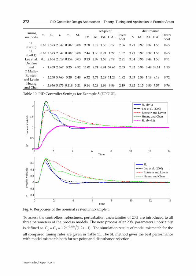
providing a fair comparison. The setting parameters of the other existing method are taken from Lee et al. (2000). The output responses for disturbance rejection by the various methods (Figure 6a) show that the SL method performs best. Comparison of performance and robustness matrices of the considered tuning rules (Table 10) also shows that the SL method performs best.
Responses to a unit step set-point change using 1DOF controllers (Figure 6b) show significant overshoots. Using a 2DOF controller can reduce the overshoot, as shown in the response of the SL method when b=0.1. Comparison of the controllers' performances (Figures 6 and Table 10) demonstrates the advantages of the SL method.
www.intechopen.com
PID Controller Design Approaches – Theory, Tuning and Application to Frontier Areas
272
Tuning methods
τc Kc τI τD Ms
set-point disturbance
TV IAE ISE ITAEOvershoot
TV IAE ISE ITAE Overs hoot
SL (b=1.0)
0.63 2.573 2.042 0.207 3.08 9.58 2.12 1.56 3.17 2.06 3.71 0.92 0.37 1.55 0.65
SL (b=0.1) 0.63 2.573 2.042 0.207 3.08 2.44 1.30 0.91 1.27 1.07 3.71 0.92 0.37 1.55 0.65
Lee et al. 0.5 2.634 2.519 0.154 3.03 9.13 2.09 1.68 2.79 2.21 3.54 0.96 0.44 1.50 0.71 De Paor
and O Malley
- 1.459 2.667 0.25 4.92 11.01 8.74 6.94 57.66 2.53 7.02 5.96 3.49 39.14 1.13
Rotstein and Lewin
- 2.250 5.760 0.20 2.48 6.32 3.74 2.28 11.24 1.82 3.03 2.56 1.18 8.19 0.72
Huang and Chen
- 2.636 5.673 0.118 3.21 9.14 3.28 1.96 9.86 2.19 3.62 2.15 0.80 7.57 0.76
Table 10. PID Controller Settings for Example 5 (FODUP)
0 2 4 6 8 10 12 140
0.5
1
1.5
2
Time
Pro
cess
Var
iabl
e
0 2 4 6 8 10 12 14
-0.4
-0.2
0
0.2
0.4
0.6
Time
Pro
cess
Var
iabl
e
SL (b=1)Lee et al. (2000) Rotstein and LewinHuang and ChenSL (b=0.1)
SLLee et al. (2000) Rotstein and LewinHuang and Chen
b
a
Fig. 6. Responses of the nominal system in Example 5.
To assess the controllers' robustness, perturbation uncertainties of 20% are introduced to all three parameters of the process models. The new process after 20% parameters uncertainty
is defined as 0.481.2 (1.2 1)sp dG G e s . The simulation results of model mismatch for the
all compared tuning rules are given in Table 11. The SL method gives the best performance with model mismatch both for set-point and disturbance rejection.
www.intechopen.com
IMC Filter Design for PID Controller Tuning of Time Delayed Processes
273
Tuning methods
set-point disturbance TV IAE ISE ITAE Overshoot TV IAE ISE ITAE Overshoot
SL (b=1.0) 14.90 2.11 1.89 2.95 2.45 5.63 0.86 0.42 1.42 0.76 Lee et al. 17.49 2.51 2.27 4.31 2.58 6.49 1.03 0.51 1.98 0.82
De Paor and O Malley
7.38 5.62 4.33 23.86 2.31 4.79 3.95 2.45 17.23 1.08
Rotstein and Lewin
7.97 3.48 2.01 10.89 2.05 3.69 2.56 1.09 9.28 0.83
Huang and Chen
18.29 3.24 2.41 9.71 2.49 6.90 2.15 0.84 8.35 0.86
Table 11. Robustness Analysis for Example 5 (FODUP)0.481.2
1.2 1
s
p de
G Gs
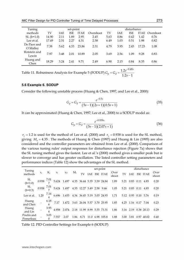
5.6 Example 6. SODUP
Consider the following unstable process (Huang & Chen, 1997, and Lee et al., 2000):
0.5
5 1 2 1 0.5 1
s
p de
G Gs s s
(35)
It can be approximated (Huang & Chen, 1997; Lee et al., 2000) to a SODUP model as:
0.939
5 1 2.07 1
s
p de
G Gs s
(36)
1.2c is used for the method of Lee et al. (2000) and 0.938c is used for the SL method, giving 4.35sM . The methods of Huang & Chen (1997) and Huang & Lin (1995) are also considered and the controller parameters are obtained from Lee et al. (2000). Comparison of the various tuning rules' output responses for disturbance rejection (Figure 7a) shows that the SL tuning method gives the fastest. Lee et al.’s (2000) method gives a smaller peak but is slower to converge and has greater oscillation. The listed controller setting parameters and performance indices (Table 12) show the advantages of the SL method.
Tuning methods
τc Kc τI τD Ms
set-point disturbance
TV IAE ISE ITAEOver shoot
TV IAE ISE ITAE Over shoot
SL (b=1.0) 0.938
7.017 5.624 1.497 4.35 36.44 5.35 3.59 24.84 1.89 5.21 0.85 0.11 4.85 0.20
SL (b=0.3)
0.938 7.017
5.624 1.497 4.35 12.27 3.49 2.58 9.46 1.05 5.21 0.85 0.11 4.85 0.20
Lee et al. 1.20 7.14
4 6.696 1.655 4.34 36.45 5.19 3.03 24.93 1.71 5.12 0.95 0.10 5.76 0.19
Huang and Chen -
6.186 7.17 1.472 3.63 26.04 5.57 3.70 25.95 1.85 4.25 1.16 0.17 7.04 0.23
Huang and Lin
- 3.954
4.958 2.074 2.18 11.99 8.99 5.55 73.31 1.86 3.16 2.19 0.38 20.13 0.29
Poulin and Pomerleau
- 3.05
0 7.557 2.07 1.86 8.71 11.0 6.98 105.8 1.88 3.00 3.81 0.97 40.02 0.40
Table 12. PID Controller Settings for Example 6 (SODUP)
www.intechopen.com
PID Controller Design Approaches – Theory, Tuning and Application to Frontier Areas
274
0 5 10 15 20 250
0.5
1
1.5
2
Time
Pro
cess
Var
iabl
e
0 5 10 15 20 25-0.1
0
0.1
0.2
0.3
Time
Pro
cess
Var
iabl
e
SL (b=1)Lee et al. (2000) Huang and ChenHuang and LinSL (b=0.3)
SL (b=1)Lee et al. (2000) Huang and ChenHuang and Lin
a
b
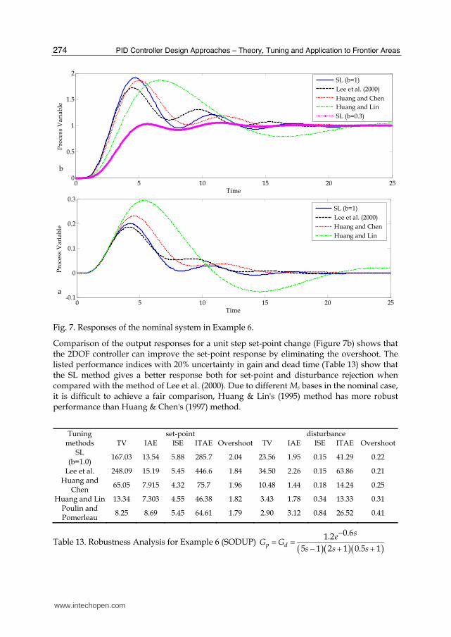
Fig. 7. Responses of the nominal system in Example 6.
Comparison of the output responses for a unit step set-point change (Figure 7b) shows that the 2DOF controller can improve the set-point response by eliminating the overshoot. The listed performance indices with 20% uncertainty in gain and dead time (Table 13) show that the SL method gives a better response both for set-point and disturbance rejection when compared with the method of Lee et al. (2000). Due to different Ms bases in the nominal case, it is difficult to achieve a fair comparison, Huang & Lin's (1995) method has more robust performance than Huang & Chen's (1997) method.
Tuning
methods set-point disturbance
TV IAE ISE ITAE Overshoot TV IAE ISE ITAE Overshoot SL
(b=1.0) 167.03 13.54 5.88 285.7 2.04 23.56 1.95 0.15 41.29 0.22
Lee et al. 248.09 15.19 5.45 446.6 1.84 34.50 2.26 0.15 63.86 0.21 Huang and
Chen 65.05 7.915 4.32 75.7 1.96 10.48 1.44 0.18 14.24 0.25
Huang and Lin 13.34 7.303 4.55 46.38 1.82 3.43 1.78 0.34 13.33 0.31 Poulin and Pomerleau 8.25 8.69 5.45 64.61 1.79 2.90 3.12 0.84 26.52 0.41
Table 13. Robustness Analysis for Example 6 (SODUP) 0.61.2
5 1 2 1 0.5 1p d
seG G
s s s
www.intechopen.com

IMC Filter Design for PID Controller Tuning of Time Delayed Processes
275
6. Discussions
6.1 Effects of 訴c on tuning parameters
The SL IMC-PID tuning method has a single tuning parameter, 訴c, that is related to the closed-loop performance and the robustness of the control system. It is important to analyze the effects of 訴c on the PID parameters, Kc , 訴I and 訴D. Consider the FOPDT model:
1
s
p de
G Gs
(37)
The PID parameters are calculated using the SL method for different values of the closed-loop time constant, 訴c, for each case of θ/τ= 0.25, 0.5, 0.75 and 1.0.
As the θ/τ ratio decreases, the effect of 訴c on Kc is increases (Figure 8), implying that Kc becomes less sensitive to 訴c with increasing θ/τ ratio. As 訴c increases, the variation of Kc decreases significantly.
Fig. 8. Proportional gain (Kc) settings with respect to 訴c
www.intechopen.com

PID Controller Design Approaches – Theory, Tuning and Application to Frontier Areas
276 訴I increases initially with increasing 訴c for the different θ/τ ratios, but as the θ/τ ratio increases from 0.25 to 1.0, the variation of 訴I decreases, as clearly demonstrated at θ/τ =1.0 (Figure 9). The trend of increasing 訴I with 訴c reverses after a specific 訴c value for each θ/τ ratio. For the considered θ/τ ratios, 訴I decreases with increasing 訴c after a certain value of 訴c, which increases as θ/τ ratio increases. Note that for some large values of 訴c, 訴I is positive.
In Figure 10, the variation of 訴D with 訴c is shown and it is clear from figure that the 訴D remains positive with increasing 訴c at the various considered θ/τ ratios.
Fig. 9. Integral time constant (訴I) settings at different 訴c values
6.2 訴c guidelines for the IMC-PID parameter settings
Since the closed-loop time constant, 訴c, is the only user-defined tuning parameter in the SL tuning rules, it is important to have some 訴c guidelines to provide the best performance with
www.intechopen.com

IMC Filter Design for PID Controller Tuning of Time Delayed Processes
277
a given robustness level. Figure 11 shows the plot of 訴c/訴 vs. θ/訴 ratios for the FOPDT model at different Ms values. Figure 12 shows the 訴c guideline plot for the DIP model, where 訴c can be calculated for a desired θ value at different Ms values. Figure 13 shows the 訴c guidelines for the SOPDT model; Skogestad’s half rule is used to obtain this 訴c/訴 vs. θ/訴
plot. A SOPDT can be converted to a FOPDT model using the half rule. For any given θ/訴 ratio of the converted FOPDT model, it is possible to obtain the 訴c/訴 value from the plot in Figure 13 for the SOPDT. Although this model reduction technique introduces some approximation error, it is within an acceptable limit. Figures 14 and 15 show the 訴c guideline plots for the FODIP and FODUP models, respectively.
Fig. 10. Derivative time constant (訴D) settings with respect to 訴c
www.intechopen.com

PID Controller Design Approaches – Theory, Tuning and Application to Frontier Areas
278
Fig. 11. 訴c guidelines for a FOPDT
Fig. 12. 訴c guidelines for a DIP
www.intechopen.com

IMC Filter Design for PID Controller Tuning of Time Delayed Processes
279
Fig. 13. 訴c guidelines for a SOPDT
Fig. 14. 訴c guidelines for a FODIP
www.intechopen.com

PID Controller Design Approaches – Theory, Tuning and Application to Frontier Areas
280
Fig. 15. 訴c guidelines for a FODUP
6.3 Beneficial range of the SL method
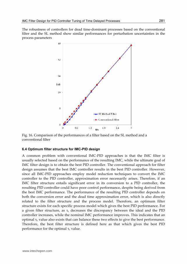
The load performance of the SL PID controller is superior as a lag time dominates but its superiority over a controller based on a conventional filter diminishes as a dead time dominates. In the case of a dead time-dominant process (i.e. 1 ), the filter time constant should be chosen for stability as . Therefore, the process pole at -1/τ is not a dominant pole in the closed-loop system. Instead, the pole at -1/τc determines the overall dynamics. Thus, introducing a lead term, 1s , to the filter to compensate the process pole at -1/τ has little impact on the speed of the disturbance rejection response. The lead term generally increases the complexity of the IMC controller, which in turn degrades the performance of the resulting controller by causing a large discrepancy between the ideal and the PID controllers. It is also important to note that as the order of the filter increases, the power of the denominator, (τcs+1), also increases, causing an unnecessarily slow output response. As a result in the case of a dead time-dominant process, a conventional filter without any lead term could be advantageous. Comparison of the IAE values of the load responses of the PID controllers based on the SL filter and on the conventional filter for the process model, 10 ( 1)s
p dG G e s , clearly indicates that the IAE gap between the two filters decreases as the θ/τ ratio increases (Figure 16).
www.intechopen.com
IMC Filter Design for PID Controller Tuning of Time Delayed Processes
281
The robustness of controllers for dead time-dominant processes based on the conventional filter and the SL method show similar performances for perturbation uncertainties in the process parameters
Fig. 16. Comparison of the performances of a filter based on the SL method and a conventional filter
6.4 Optimum filter structure for IMC-PID design
A common problem with conventional IMC-PID approaches is that the IMC filter is usually selected based on the performance of the resulting IMC, while the ultimate goal of IMC filter design is to obtain the best PID controller. The conventional approach for filter design assumes that the best IMC controller results in the best PID controller. However, since all IMC-PID approaches employ model reduction techniques to convert the IMC controller to the PID controller, approximation error necessarily arises. Therefore, if an IMC filter structure entails significant error in its conversion to a PID controller, the resulting PID controller could have poor control performance, despite being derived from the best IMC performance. The performance of the resulting PID controller depends on both the conversion error and the dead time approximation error, which is also directly related to the filter structure and the process model. Therefore, an optimum filter structure exists for each specific process model which gives the best PID performance. For a given filter structure, as τc decreases the discrepancy between the ideal and the PID controller increases, while the nominal IMC performance improves. This indicates that an optimal τc value also exists that can balance these two effects to give the best performance. Therefore, the best filter structure is defined here as that which gives the best PID performance for the optimal τc value.
www.intechopen.com

PID Controller Design Approaches – Theory, Tuning and Application to Frontier Areas
282
To find the optimum filter structure, IMC filters with structures of 1 1 r nrcs s
for the first order models and of 222 1 c1 1
r r ns s s for the second order
models are evaluated, where r and n are each varied from 0 to 2. A high order filter structure is then generally shown to give a better PID performance than a low order filter structure. For example, for an FOPDT model, the high order filter,
32c1 1f s s s , provides the best disturbance rejection in terms of IAE. Based
on the optimum filter structures, PID controller tuning rules are derived for several representative process models (Table 1).
Fig. 17. τc vs. IAE for various tuning rules for a FOPDT
Figure 17 shows the variation of IAE with τc for the tuning methods of the FOPDT model considered in example 1. The tuning rules proposed by Horn et al. (1996) and Lee et al.
(1998) are based on the same filter 2c1 1f s s s . Horn et al. (1996) use a 1/1
www.intechopen.com

IMC Filter Design for PID Controller Tuning of Time Delayed Processes
283
Pade approximation for the dead time when calculating both β and the PID parameters. Lee et al. (1998) obtained the PID parameters using a Maclaurin series approximation. Since both methods use the same IMC filter structure, the IMC controllers of Lee et al. (1998) and Horn
et al. (1996) coincide with each other (Figure 17). Due to the approximation error in se when calculating the PID, the performance of Lee et al.'s (1998) method is better than that of Horn et al. (1996). Down to some optimum τc value, the ideal (or IMC) and the PID controllers have no significant difference in performance; after some minimum IAE point, the gap increases sharply towards the limit of instability. The smallest IAE value can be achieved by the SL tuning method while that of Horn et al. (1996) shows the worst performance. The SL method also performs best in the case of model mismatch where a large τc value is required.
It is worthwhile to visualize the performance and robustness of the controller design. Plotting the Ms robustness index with respect to the IAE performance index for the different tuning methods for the FOPDT model of Example 1 (Figure 18) shows that at any given Ms, the PID controller developed by the SL method always produces a lower IAE than those by the other tuning rules.
Fig. 18. Ms vs. IAE for different tuning rules for a FOPDT
www.intechopen.com

PID Controller Design Approaches – Theory, Tuning and Application to Frontier Areas
284
7. Conclusions
The SL method could produce optimum IMC filter structures for several representative process models to improve the PID controllers' disturbance rejection. The method's filter structures could be used to derive tuning rules for the PID controllers using the generalized IMC-PID method. Simulation results demonstrate the superiority of the SL method when various controllers are compared by each being tuned to have the same degree of robustness in terms of maximum sensitivity. The SL method is more beneficial as the process is lag time-dominant. Robustness analysis, by inserting a 20% perturbation in each of the process parameters in the worst direction, demonstrates the robustness of the SL method against parameter uncertainty. Closed-loop time constant, τc, guidelines are also proposed by the SL method for several process models over a wide range of θ/τ ratios.
8. Acknowledgment
The authors gratefully acknowledge the funding support provided by the Deanship of Scientific Research at King Fahd University of Petroleum & Minerals (project No. SB101016).
9. References
Åström, K. J., Hägglund, T. (1984). Automatic tuning of simple regulators with specifications on phase and amplitude margins, Automatica, 20, pp.645–651.
Åström, K.J., Panagopoulos, H., Hägglund, T. (1998). Design of PI controllers based on non-convex optimization. Automatica, 34, pp.585-601.
Åström, K. J., Hägglund, T.(1995). PID controllers: Theory, Design, and Tuning, 2nd ed,; Instrument Society of America: Research Triangle Park, NC.
Chen, D., Seborg, D. E. (2002). PI/PID controller design based on direct synthesis and disturbance rejection. Ind. Eng. Chem. Res., 41, pp. 4807-4822.
Chien, I.-L., Fruehauf, P. S. (1990). Consider IMC tuning to improve controller performance. Chem. Eng. Prog. 1990, 86, pp.33.
De Paor, A. M., (1989). Controllers of Ziegler Nichols type for unstable process with time delay. International Journal of Control, 49, pp.1273.
Desborough, L. D., Miller, R.M. (2002). Increasing customer value of industrial control performance monitoring—Honeywell’s experience. Chemical Process Control –VI (Tuscon, Arizona, Jan. 2001), AIChE Symposium Series No. 326. Volume 98, USA.
Horn, I. G., Arulandu, J. R., Christopher, J. G., VanAntwerp, J. G., Braatz, R. D.(1996). Improved filter design in internal model control. Ind. Eng. Chem. Res. 35, pp.3437.
Huang, C. T., Lin, Y. S. (1995). Tuning PID controller for open-loop unstable processes with time delay. Chem. Eng. Communications, 133, pp.11.
Huang, H. P., Chen, C. C. (1997). Control-system synthesis for open-loop unstable process with time delay. IEE Process-Control Theory and Application, 144, pp.334.
www.intechopen.com

IMC Filter Design for PID Controller Tuning of Time Delayed Processes
285
Kano, M., Ogawa, M. (2010). The state of the art in chemical process control in Japan: Good practice and questionnaire survey, Journal of Process Control, 20, pp. 968-982.
Lee, Y., Lee, J., Park, S. (2000). PID controller tuning for integrating and unstable processes with time delay. Chem. Eng. Sci., 55, pp. 3481-3493.
Lee, Y., Park, S., Lee, M., Brosilow, C. (1998). PID controller tuning for desired closed-loop responses for SI/SO systems. AIChE J. 44, pp.106-115.
Morari, M., Zafiriou, E. (1989). Robust Process Control; Prentice-Hall: Englewood Cliffs, NJ. Poulin, ED., Pomerleau, A. (1996). PID tuning for integrating and unstable processes. IEE
Process Control Theory and Application, 143(5), pp.429. Rivera, D. E., Morari, M., Skogestad, S.(1986). Internal model control. 4. PID controller
design. Ind. Eng. Chem. Process Des. Dev., 25, pp.252. Rotstein, G. E., Lewin, D. R. (1992). Control of an unstable batch chemical reactor. Computers
in Chem. Eng., 16 (1), pp.27. Schei, T. S.(1992). A method for closed loop automatic tuning of PID controllers,
Automatica, 20, 3, pp. 587-591. Seborg, D. E., Edgar, T. F., Mellichamp, D. A. (2004). Process dynamics and control, 2nd ed.,
John Wiley & Sons, New York, U.S.A. Seki, H., Shigemasa, T. (2010). Retuning oscillatory PID control loops based on plant
operation data, Journal of Process Control, 20, pp. 217-227. Shamsuzzoha, M., Lee, M. (2007a). An enhanced performance PID.filter controller for first
order time delay processes, Journal of Chemical Engineering of Japan, 40, No. 6, pp.501-510.
Shamsuzzoha, M., Lee, M. (2007b). IMC-PID controller design for improved disturbance rejection, Ind. Eng. Chem. Res., 46, No. 7, pp. 2077-2091.
Shamsuzzoha, M., Lee, M. (2008a). Analytical design of enhanced PID.filter controller for integrating and first order unstable processes with time delay, Chemical Engineering Science, 63, pp. 2717-2731.
Shamsuzzoha, M., Lee, M. (2008b). Design of advanced PID controller for enhanced disturbance rejection of second order process with time delay, AIChE, 54, No. 6, pp. 1526-1536.
Shamsuzzoha, M., Skogestad, S. (2010a). Internal report with additional data for the set-point overshoots method, Available at the home page of S. Skogestad. http://www.nt.ntnu.no/users/skoge/.
Shamsuzzoha, M., Skogestad, S. (2010b). The set-point overshoot method: A simple and fast closed-loop approch for PI tuning, Journal of Process Control 20, pp. 1220–1234.
Skogestad, S. (2003). Simple analytic rules for model reduction and PID controller tuning. J. Process Control, 13, pp.291-309.
Smith, C. L., Corripio, A. B., Martin, J. (1975). Controller tuning from simple process models. Instrum. Technol. 1975, 22 (12), 39.
Tyreus, B.D., Luyben, W.L. (1992). Tuning PI controllers for integrator/dead time processes, Ind. Eng. Chem. Res., pp.2625–2628.
Veronesi, M., Visioli, A. (2010). Performance assessment and retuning of PID controllers for integral processes, Journal of Process Control, 20, pp. 261-269.
www.intechopen.com

PID Controller Design Approaches – Theory, Tuning and Application to Frontier Areas
286
Yuwana, M., Seborg, D. E. (1982). A new method for on-line controller tuning, AIChE
Journal, 28 (3), pp. 434-440. Ziegler, J. G., Nichols, N. B. (1942). Optimum settings for automatic controllers. Trans.
ASME, 64, 759-768.
www.intechopen.com
PID Controller Design Approaches - Theory, Tuning andApplication to Frontier AreasEdited by Dr. Marialena Vagia
ISBN 978-953-51-0405-6Hard cover, 286 pagesPublisher InTechPublished online 28, March, 2012Published in print edition March, 2012
InTech EuropeUniversity Campus STeP Ri Slavka Krautzeka 83/A 51000 Rijeka, Croatia Phone: +385 (51) 770 447 Fax: +385 (51) 686 166www.intechopen.com
InTech ChinaUnit 405, Office Block, Hotel Equatorial Shanghai No.65, Yan An Road (West), Shanghai, 200040, China
Phone: +86-21-62489820 Fax: +86-21-62489821
First placed on the market in 1939, the design of PID controllers remains a challenging area that requires newapproaches to solving PID tuning problems while capturing the effects of noise and process variations. Theaugmented complexity of modern applications concerning areas like automotive applications, microsystemstechnology, pneumatic mechanisms, dc motors, industry processes, require controllers that incorporate intotheir design important characteristics of the systems. These characteristics include but are not limited to:model uncertainties, system's nonlinearities, time delays, disturbance rejection requirements and performancecriteria. The scope of this book is to propose different PID controllers designs for numerous moderntechnology applications in order to cover the needs of an audience including researchers, scholars andprofessionals who are interested in advances in PID controllers and related topics.
How to referenceIn order to correctly reference this scholarly work, feel free to copy and paste the following:
M. Shamsuzzoha and Moonyong Lee (2012). IMC Filter Design for PID Controller Tuning of Time DelayedProcesses, PID Controller Design Approaches - Theory, Tuning and Application to Frontier Areas, Dr.Marialena Vagia (Ed.), ISBN: 978-953-51-0405-6, InTech, Available from:http://www.intechopen.com/books/pid-controller-design-approaches-theory-tuning-and-application-to-frontier-areas/imc-filter-design-for-pid-controller-tuning-for-time-delayed-processes

© 2012 The Author(s). Licensee IntechOpen. This is an open access articledistributed under the terms of the Creative Commons Attribution 3.0License, which permits unrestricted use, distribution, and reproduction inany medium, provided the original work is properly cited.


![[PID] PID Control - Good Tuning - A Pocket Guide](https://static.fdocuments.in/doc/165x107/577d2a661a28ab4e1ea914b1/pid-pid-control-good-tuning-a-pocket-guide.jpg)