ImageJ User Guide · user-guide.zip. Printable booklets Two-sided booklets that can be printed on a...

ImageJUser Guide

IJ 1.45

Contents

Release Notes for ImageJ 1.45m vii

Noteworthy viii

Macro Listings ix

Guide Conventions x

I Getting Started

1 What is ImageJ? 1

2 Installing and Maintaining ImageJ 22.1 ImageJ Distributions . . . . . . . . . . . . . . . . . . . . . . . . . . . . . . . . 22.2 Software Packages Built on Top of ImageJ . . . . . . . . . . . . . . . . . . . . 32.3 ImageJ2 . . . . . . . . . . . . . . . . . . . . . . . . . . . . . . . . . . . . . . . 4

3 Getting Help 43.1 Help on Image Analysis . . . . . . . . . . . . . . . . . . . . . . . . . . . . . . . 43.2 Help on ImageJ . . . . . . . . . . . . . . . . . . . . . . . . . . . . . . . . . . . 5

II Working with ImageJ

4 Using Keyboard Shortcuts 8

5 Finding Commands 9

6 Undo and Redo 9

7 Image Types and Formats 10

8 Stacks, Virtual Stacks and Hyperstacks 11

9 Color Images 13

10 Selections 17

11 Settings and Preferences 19

III Extending ImageJ

12 Macros 20

13 Scripts 21

14 Plugins 21

15 Scripting in Other Languages 22

16 Running ImageJ From the Command Line 23

ii

17 ImageJ Interoperability 24

IV ImageJ User Interface

18 Tools18.1 Area Selection Tools . . . . . . . . . . . . . . . . . . . . . . . . . . . . . . . . 2618.2 Line Selection Tools . . . . . . . . . . . . . . . . . . . . . . . . . . . . . . . . . 2818.3 Arrow Tool . . . . . . . . . . . . . . . . . . . . . . . . . . . . . . . . . . . . . . 2918.4 Angle Tool . . . . . . . . . . . . . . . . . . . . . . . . . . . . . . . . . . . . . . 3018.5 Point Tool . . . . . . . . . . . . . . . . . . . . . . . . . . . . . . . . . . . . . . 3018.6 Multi-point Tool . . . . . . . . . . . . . . . . . . . . . . . . . . . . . . . . . . . 3018.7 Wand Tool . . . . . . . . . . . . . . . . . . . . . . . . . . . . . . . . . . . . . . . 3118.8 Text Tool . . . . . . . . . . . . . . . . . . . . . . . . . . . . . . . . . . . . . . . 3118.9 Magnifying Glass . . . . . . . . . . . . . . . . . . . . . . . . . . . . . . . . . . 3218.10 Scrolling Tool . . . . . . . . . . . . . . . . . . . . . . . . . . . . . . . . . . . . 3218.11 Color Picker . . . . . . . . . . . . . . . . . . . . . . . . . . . . . . . . . . . . . 3218.12 Toolset Switcher . . . . . . . . . . . . . . . . . . . . . . . . . . . . . . . . . . . 3318.13 Macro Tools . . . . . . . . . . . . . . . . . . . . . . . . . . . . . . . . . . . . . 33

19 Contextual Menu 34

20 Results Table 35

21 ImageJ Editor 36

22 Log Window 38

V Menu Commands

23 File . 4023.1 New . . . . . . . . . . . . . . . . . . . . . . . . . . . . . . . . . . . . . . . . . . 4023.2 Open. . . . . . . . . . . . . . . . . . . . . . . . . . . . . . . . . . . . . . . . . . . 4123.3 Open Next [O] . . . . . . . . . . . . . . . . . . . . . . . . . . . . . . . . . . . . . 4123.4 Open Samples . . . . . . . . . . . . . . . . . . . . . . . . . . . . . . . . . . . . . 4123.5 Open Recent . . . . . . . . . . . . . . . . . . . . . . . . . . . . . . . . . . . . . 4223.6 Import . . . . . . . . . . . . . . . . . . . . . . . . . . . . . . . . . . . . . . . . 4223.7 Close [w] . . . . . . . . . . . . . . . . . . . . . . . . . . . . . . . . . . . . . . . 4623.8 Close All . . . . . . . . . . . . . . . . . . . . . . . . . . . . . . . . . . . . . . . 4623.9 Save [s] . . . . . . . . . . . . . . . . . . . . . . . . . . . . . . . . . . . . . . . . 4623.10 Save As . . . . . . . . . . . . . . . . . . . . . . . . . . . . . . . . . . . . . . . . 4623.11 Revert [r] . . . . . . . . . . . . . . . . . . . . . . . . . . . . . . . . . . . . . . . 5023.12 Page Setup. . . . . . . . . . . . . . . . . . . . . . . . . . . . . . . . . . . . . . . 5023.13 Print. . . [p] . . . . . . . . . . . . . . . . . . . . . . . . . . . . . . . . . . . . . . 5023.14 Quit . . . . . . . . . . . . . . . . . . . . . . . . . . . . . . . . . . . . . . . . . . 50

24 Edit . 5124.1 Undo [z] . . . . . . . . . . . . . . . . . . . . . . . . . . . . . . . . . . . . . . . . 5124.2 Cut [x] . . . . . . . . . . . . . . . . . . . . . . . . . . . . . . . . . . . . . . . . . 5124.3 Copy [c] . . . . . . . . . . . . . . . . . . . . . . . . . . . . . . . . . . . . . . . . . 5124.4 Copy to System . . . . . . . . . . . . . . . . . . . . . . . . . . . . . . . . . . . . 5124.5 Paste [v] . . . . . . . . . . . . . . . . . . . . . . . . . . . . . . . . . . . . . . . . 51

iii

The

IJUser

Guid

e—

Bookle

t1

24.6 Paste Control. . . . . . . . . . . . . . . . . . . . . . . . . . . . . . . . . . . . . . . 5124.7 Clear . . . . . . . . . . . . . . . . . . . . . . . . . . . . . . . . . . . . . . . . . 5224.8 Clear Outside . . . . . . . . . . . . . . . . . . . . . . . . . . . . . . . . . . . . . 5224.9 Fill [f] . . . . . . . . . . . . . . . . . . . . . . . . . . . . . . . . . . . . . . . . . 5224.10 Draw [d] . . . . . . . . . . . . . . . . . . . . . . . . . . . . . . . . . . . . . . . 5224.11 Invert [I] . . . . . . . . . . . . . . . . . . . . . . . . . . . . . . . . . . . . . . . 5324.12 Selection . . . . . . . . . . . . . . . . . . . . . . . . . . . . . . . . . . . . . . . 5324.13 Options . . . . . . . . . . . . . . . . . . . . . . . . . . . . . . . . . . . . . . . . 57

25 Image . 6425.1 Type . . . . . . . . . . . . . . . . . . . . . . . . . . . . . . . . . . . . . . . . . 6425.2 Adjust . . . . . . . . . . . . . . . . . . . . . . . . . . . . . . . . . . . . . . . . 6425.3 Show Info. . . [i] . . . . . . . . . . . . . . . . . . . . . . . . . . . . . . . . . . . . 7125.4 Properties. . . [P] . . . . . . . . . . . . . . . . . . . . . . . . . . . . . . . . . . . 7225.5 Color . . . . . . . . . . . . . . . . . . . . . . . . . . . . . . . . . . . . . . . . . 7225.6 Stacks . . . . . . . . . . . . . . . . . . . . . . . . . . . . . . . . . . . . . . . . 7525.7 Hyperstacks . . . . . . . . . . . . . . . . . . . . . . . . . . . . . . . . . . . . . 8425.8 Crop [X] . . . . . . . . . . . . . . . . . . . . . . . . . . . . . . . . . . . . . . . 8525.9 Duplicate. . . [D] . . . . . . . . . . . . . . . . . . . . . . . . . . . . . . . . . . . 8625.10 Rename. . . . . . . . . . . . . . . . . . . . . . . . . . . . . . . . . . . . . . . . . 8625.11 Scale. . . [E] . . . . . . . . . . . . . . . . . . . . . . . . . . . . . . . . . . . . . . 8625.12 Transform . . . . . . . . . . . . . . . . . . . . . . . . . . . . . . . . . . . . . . 8725.13 Zoom . . . . . . . . . . . . . . . . . . . . . . . . . . . . . . . . . . . . . . . . . 8825.14 Overlay . . . . . . . . . . . . . . . . . . . . . . . . . . . . . . . . . . . . . . . . 8925.15 Lookup Tables . . . . . . . . . . . . . . . . . . . . . . . . . . . . . . . . . . . . . 91

26 Process . 9326.1 Smooth [S] . . . . . . . . . . . . . . . . . . . . . . . . . . . . . . . . . . . . . . 9326.2 Sharpen . . . . . . . . . . . . . . . . . . . . . . . . . . . . . . . . . . . . . . . . 9326.3 Find Edges . . . . . . . . . . . . . . . . . . . . . . . . . . . . . . . . . . . . . . . 9326.4 Find Maxima. . . . . . . . . . . . . . . . . . . . . . . . . . . . . . . . . . . . . . 9326.5 Enhance Contrast . . . . . . . . . . . . . . . . . . . . . . . . . . . . . . . . . . 9526.6 Noise . . . . . . . . . . . . . . . . . . . . . . . . . . . . . . . . . . . . . . . . . 9626.7 Shadows . . . . . . . . . . . . . . . . . . . . . . . . . . . . . . . . . . . . . . . 9726.8 Binary . . . . . . . . . . . . . . . . . . . . . . . . . . . . . . . . . . . . . . . . 9826.9 Math . . . . . . . . . . . . . . . . . . . . . . . . . . . . . . . . . . . . . . . . . 10226.10 FFT . . . . . . . . . . . . . . . . . . . . . . . . . . . . . . . . . . . . . . . . . . 10526.11 Filters . . . . . . . . . . . . . . . . . . . . . . . . . . . . . . . . . . . . . . . . . 10926.12 Batch . . . . . . . . . . . . . . . . . . . . . . . . . . . . . . . . . . . . . . . . . . 11126.13 Image Calculator. . . . . . . . . . . . . . . . . . . . . . . . . . . . . . . . . . . . 11326.14 Subtract Background. . . . . . . . . . . . . . . . . . . . . . . . . . . . . . . . . . 11426.15 Repeat Command [R] . . . . . . . . . . . . . . . . . . . . . . . . . . . . . . . . 116

27 Analyze . 11727.1 Measure. . . [m] . . . . . . . . . . . . . . . . . . . . . . . . . . . . . . . . . . . . 11727.2 Analyze Particles. . . . . . . . . . . . . . . . . . . . . . . . . . . . . . . . . . . . 11727.3 Summarize . . . . . . . . . . . . . . . . . . . . . . . . . . . . . . . . . . . . . . 12027.4 Distribution. . . . . . . . . . . . . . . . . . . . . . . . . . . . . . . . . . . . . . . 12027.5 Label . . . . . . . . . . . . . . . . . . . . . . . . . . . . . . . . . . . . . . . . . . 12127.6 Clear Results . . . . . . . . . . . . . . . . . . . . . . . . . . . . . . . . . . . . . . 12127.7 Set Measurements. . . . . . . . . . . . . . . . . . . . . . . . . . . . . . . . . . . . 12127.8 Set Scale. . . . . . . . . . . . . . . . . . . . . . . . . . . . . . . . . . . . . . . . 124

iv

27.9 Calibrate. . . . . . . . . . . . . . . . . . . . . . . . . . . . . . . . . . . . . . . . 12527.10 Histogram [h] . . . . . . . . . . . . . . . . . . . . . . . . . . . . . . . . . . . . . 12627.11 Plot Profile [k] . . . . . . . . . . . . . . . . . . . . . . . . . . . . . . . . . . . . 12727.12 Surface Plot. . . . . . . . . . . . . . . . . . . . . . . . . . . . . . . . . . . . . . . 12827.13 Gels . . . . . . . . . . . . . . . . . . . . . . . . . . . . . . . . . . . . . . . . . . 12927.14 Tools . . . . . . . . . . . . . . . . . . . . . . . . . . . . . . . . . . . . . . . . . 130

28 Plugins . 13828.1 Macros . . . . . . . . . . . . . . . . . . . . . . . . . . . . . . . . . . . . . . . . 13828.2 Shortcuts . . . . . . . . . . . . . . . . . . . . . . . . . . . . . . . . . . . . . . . 13928.3 Utilities . . . . . . . . . . . . . . . . . . . . . . . . . . . . . . . . . . . . . . . 14028.4 New . . . . . . . . . . . . . . . . . . . . . . . . . . . . . . . . . . . . . . . . . . 14328.5 Compile and Run. . . . . . . . . . . . . . . . . . . . . . . . . . . . . . . . . . . . 144

29 Window . 14529.1 Show All [ ] ] . . . . . . . . . . . . . . . . . . . . . . . . . . . . . . . . . . . . . 14529.2 Put Behind [tab] . . . . . . . . . . . . . . . . . . . . . . . . . . . . . . . . . . . 14529.3 Cascade . . . . . . . . . . . . . . . . . . . . . . . . . . . . . . . . . . . . . . . . 14529.4 Tile . . . . . . . . . . . . . . . . . . . . . . . . . . . . . . . . . . . . . . . . . . 145

30 Help . 14630.1 ImageJ Website. . . . . . . . . . . . . . . . . . . . . . . . . . . . . . . . . . . . . 14630.2 ImageJ News. . . . . . . . . . . . . . . . . . . . . . . . . . . . . . . . . . . . . . 14630.3 Documentation. . . . . . . . . . . . . . . . . . . . . . . . . . . . . . . . . . . . . 14630.4 Installation. . . . . . . . . . . . . . . . . . . . . . . . . . . . . . . . . . . . . . . 14630.5 Mailing List. . . . . . . . . . . . . . . . . . . . . . . . . . . . . . . . . . . . . . . 14630.6 Dev. Resources. . . . . . . . . . . . . . . . . . . . . . . . . . . . . . . . . . . . . 14630.7 Plugins. . . . . . . . . . . . . . . . . . . . . . . . . . . . . . . . . . . . . . . . . 14630.8 Macros. . . . . . . . . . . . . . . . . . . . . . . . . . . . . . . . . . . . . . . . . 14630.9 Macro Functions. . . . . . . . . . . . . . . . . . . . . . . . . . . . . . . . . . . . 14630.10 Update ImageJ. . . . . . . . . . . . . . . . . . . . . . . . . . . . . . . . . . . . . 14730.11 Refresh Menus . . . . . . . . . . . . . . . . . . . . . . . . . . . . . . . . . . . . 14730.12 About Plugins . . . . . . . . . . . . . . . . . . . . . . . . . . . . . . . . . . . . 14730.13 About ImageJ. . . . . . . . . . . . . . . . . . . . . . . . . . . . . . . . . . . . . . 147

VI Keyboard Shortcuts

31 Key Modifiers31.1 Alt Key Modifications . . . . . . . . . . . . . . . . . . . . . . . . . . . . . . . 15031.2 Shift Key Modifications . . . . . . . . . . . . . . . . . . . . . . . . . . . . . . . 15031.3 Ctrl Key (or Cmd) Modifications . . . . . . . . . . . . . . . . . . . . . . . . . . 15131.4 Space Bar . . . . . . . . . . . . . . . . . . . . . . . . . . . . . . . . . . . . . . . 15131.5 Arrow Keys . . . . . . . . . . . . . . . . . . . . . . . . . . . . . . . . . . . . . . 151

32 Tools Shortcuts

Credits 153

ImageJ Related Publications 155

List of Abbreviations and Acronyms 162

v

The

IJUser

Guid

e—

Bookle

t2

Index 163

Colophon 167

vi

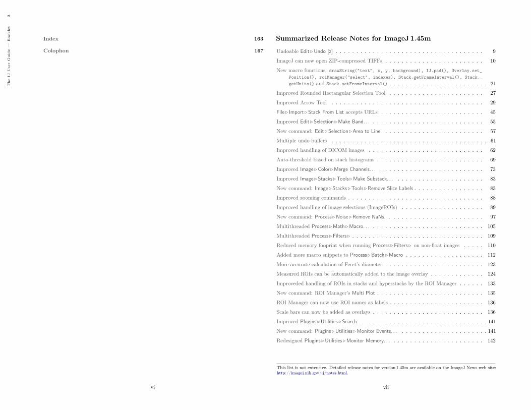
*Summarized Release Notes for ImageJ 1.45m

Undoable Edit .Undo [z] . . . . . . . . . . . . . . . . . . . . . . . . . . . . . . . . . . . . 9

ImageJ can now open ZIP-compressed TIFFs . . . . . . . . . . . . . . . . . . . . . . . . 10

New macro functions: drawString("text", x, y, background), IJ.pad(), Overlay.set_Position(), roiManager("select", indexes), Stack.getFrameInterval(), Stack._getUnits() and Stack.setFrameInterval() . . . . . . . . . . . . . . . . . . . . . . . . 21

Improved Rounded Rectangular Selection Tool . . . . . . . . . . . . . . . . . . . . . . . 27

Improved Arrow Tool . . . . . . . . . . . . . . . . . . . . . . . . . . . . . . . . . . . . . 29

File . Import .Stack From List accepts URLs . . . . . . . . . . . . . . . . . . . . . . . . . 45

Improved Edit .Selection .Make Band. . . . . . . . . . . . . . . . . . . . . . . . . . . . . . 55

New command: Edit . Selection .Area to Line . . . . . . . . . . . . . . . . . . . . . . . . 57

Multiple undo buffers . . . . . . . . . . . . . . . . . . . . . . . . . . . . . . . . . . . . . . 61

Improved handling of DICOM images . . . . . . . . . . . . . . . . . . . . . . . . . . . . 62

Auto-threshold based on stack histograms . . . . . . . . . . . . . . . . . . . . . . . . . . 69

Improved Image .Color .Merge Channels. . . . . . . . . . . . . . . . . . . . . . . . . . . . 73

Improved Image . Stacks .Tools .Make Substack. . . . . . . . . . . . . . . . . . . . . . . . 83

New command: Image . Stacks .Tools .Remove Slice Labels . . . . . . . . . . . . . . . . . 83

Improved zooming commands . . . . . . . . . . . . . . . . . . . . . . . . . . . . . . . . . 88

Improved handling of image selections (ImageROIs) . . . . . . . . . . . . . . . . . . . . 89

New command: Process .Noise .Remove NaNs. . . . . . . . . . . . . . . . . . . . . . . . . 97

Multithreaded Process .Math .Macro. . . . . . . . . . . . . . . . . . . . . . . . . . . . . . 105

Multithreaded Process .Filters . . . . . . . . . . . . . . . . . . . . . . . . . . . . . . . . . 109

Reduced memory fooprint when running Process .Filters . on non-float images . . . . . 110

Added more macro snippets to Process .Batch .Macro . . . . . . . . . . . . . . . . . . . 112

More accurate calculation of Feret’s diameter . . . . . . . . . . . . . . . . . . . . . . . . 123

Measured ROIs can be automatically added to the image overlay . . . . . . . . . . . . . 124

Improveded handling of ROIs in stacks and hyperstacks by the ROI Manager . . . . . . 133

New command: ROI Manager’s Multi Plot . . . . . . . . . . . . . . . . . . . . . . . . . . 135

ROI Manager can now use ROI names as labels . . . . . . . . . . . . . . . . . . . . . . . 136

Scale bars can now be added as overlays . . . . . . . . . . . . . . . . . . . . . . . . . . . 136

Improved Plugins .Utilities .Search. . . . . . . . . . . . . . . . . . . . . . . . . . . . . . . . 141

New command: Plugins .Utilities .Monitor Events. . . . . . . . . . . . . . . . . . . . . . . . 141

Redesigned Plugins .Utilities .Monitor Memory. . . . . . . . . . . . . . . . . . . . . . . . . 142

This list is not extensive. Detailed release notes for version 1.45m are available on the ImageJ News web site:http://imagej.nih.gov/ij/notes.html.

vii

The

IJUser

Guid

e—

Bookle

t3

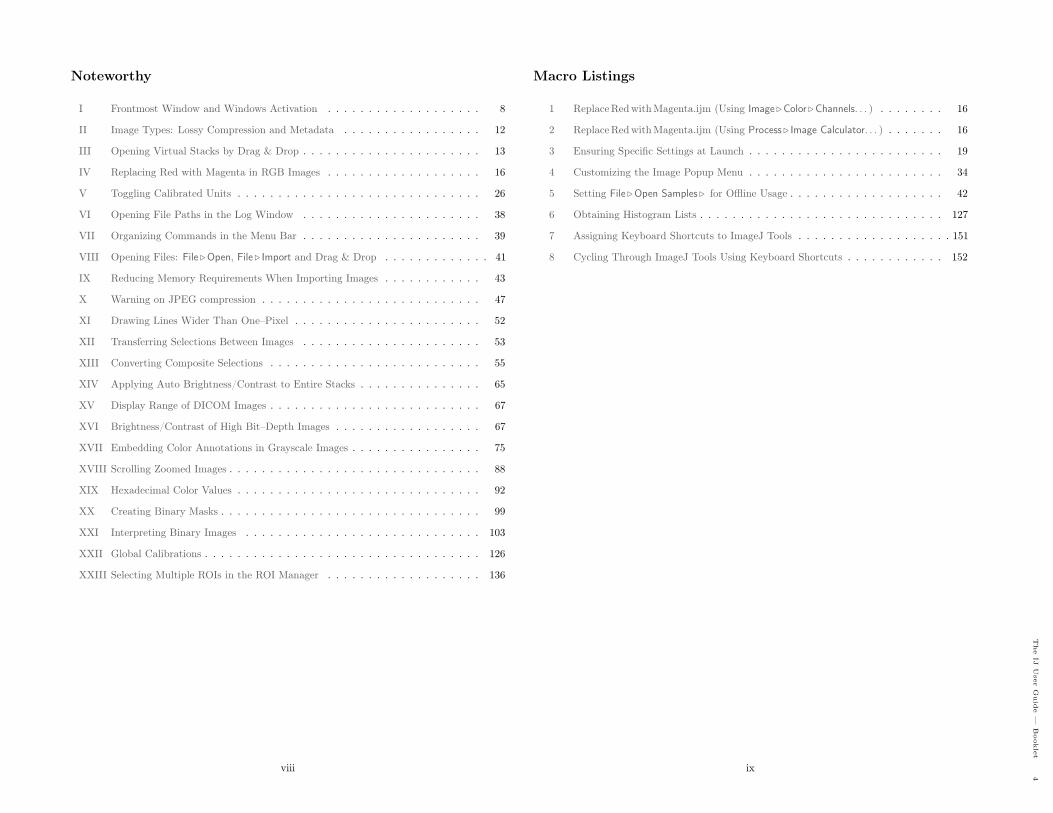
Noteworthy

I Frontmost Window and Windows Activation . . . . . . . . . . . . . . . . . . . 8

II Image Types: Lossy Compression and Metadata . . . . . . . . . . . . . . . . . 12

III Opening Virtual Stacks by Drag & Drop . . . . . . . . . . . . . . . . . . . . . . 13

IV Replacing Red with Magenta in RGB Images . . . . . . . . . . . . . . . . . . . 16

V Toggling Calibrated Units . . . . . . . . . . . . . . . . . . . . . . . . . . . . . . 26

VI Opening File Paths in the Log Window . . . . . . . . . . . . . . . . . . . . . . 38

VII Organizing Commands in the Menu Bar . . . . . . . . . . . . . . . . . . . . . . 39

VIII Opening Files: File .Open, File . Import and Drag & Drop . . . . . . . . . . . . . 41

IX Reducing Memory Requirements When Importing Images . . . . . . . . . . . . 43

X Warning on JPEG compression . . . . . . . . . . . . . . . . . . . . . . . . . . . 47

XI Drawing Lines Wider Than One–Pixel . . . . . . . . . . . . . . . . . . . . . . . 52

XII Transferring Selections Between Images . . . . . . . . . . . . . . . . . . . . . . 53

XIII Converting Composite Selections . . . . . . . . . . . . . . . . . . . . . . . . . . 55

XIV Applying Auto Brightness/Contrast to Entire Stacks . . . . . . . . . . . . . . . 65

XV Display Range of DICOM Images . . . . . . . . . . . . . . . . . . . . . . . . . . 67

XVI Brightness/Contrast of High Bit–Depth Images . . . . . . . . . . . . . . . . . . 67

XVII Embedding Color Annotations in Grayscale Images . . . . . . . . . . . . . . . . 75

XVIII Scrolling Zoomed Images . . . . . . . . . . . . . . . . . . . . . . . . . . . . . . . 88

XIX Hexadecimal Color Values . . . . . . . . . . . . . . . . . . . . . . . . . . . . . . 92

XX Creating Binary Masks . . . . . . . . . . . . . . . . . . . . . . . . . . . . . . . . 99

XXI Interpreting Binary Images . . . . . . . . . . . . . . . . . . . . . . . . . . . . . 103

XXII Global Calibrations . . . . . . . . . . . . . . . . . . . . . . . . . . . . . . . . . . 126

XXIII Selecting Multiple ROIs in the ROI Manager . . . . . . . . . . . . . . . . . . . 136

viii

Macro Listings

1 ReplaceRedwithMagenta.ijm (Using Image .Color .Channels. . . ) . . . . . . . . 16

2 ReplaceRedwithMagenta.ijm (Using Process . Image Calculator. . . ) . . . . . . . 16

3 Ensuring Specific Settings at Launch . . . . . . . . . . . . . . . . . . . . . . . . 19

4 Customizing the Image Popup Menu . . . . . . . . . . . . . . . . . . . . . . . . 34

5 Setting File .Open Samples . for Offline Usage . . . . . . . . . . . . . . . . . . . 42

6 Obtaining Histogram Lists . . . . . . . . . . . . . . . . . . . . . . . . . . . . . . 127

7 Assigning Keyboard Shortcuts to ImageJ Tools . . . . . . . . . . . . . . . . . . . 151

8 Cycling Through ImageJ Tools Using Keyboard Shortcuts . . . . . . . . . . . . 152

ix

The

IJUser

Guid

e—

Bookle

t4

Guide Formats

This guide is available in the following formats:

Enhanced PDF Optimized for electronic viewing and highly enriched in hypertext links(see Conventions Used in this Guide). Available at http://imagej.nih.gov/ij/docs/user-guide.pdf.

HTML document available online at http://imagej.nih.gov/ij/docs/guide/. For offline us-age a downloadable ZIP archive is also available at http://imagej.nih.gov/ij/docs/user-guide.zip.

Printable booklets Two-sided booklets that can be printed on a duplex unit printer by settingthe automatic duplex mode to “short edge binding”. Two formats are available:A4 (http://imagej.nih.gov/ij/docs/user-guide-A4booklet.pdf) and letter size paper(http://imagej.nih.gov/ij/docs/user-guide-USbooklet.pdf).

Conventions Used in this Guide

Throughout the guide, internal links are displayed in gray (e.g., Part IV ImageJ User Interface).Links to external URLs, such as the ImageJ website, http://imagej.nih.gov/ij/, are displayed indark blue.

ImageJ commands are typed in sans serif typeface with respective shortcut keys flanked bysquare brackets (e.g.: Image .Duplicate. . . [D]). As explained in Using Keyboard Shortcuts thisnotation implies shift-modifiers (i.e., [D] means pressing Shift D , [d] only the D key) andassumes that Require control key for shortcuts in Edit .Options .Misc. . . is unchecked.

Useful tips and reminders are placed in ‘Noteworthy notes’ numbered with upper case romannumerals (e.g., I Frontmost Window and Windows Activation). The full list of these notes isavailable on page viii.

Filenames, directory names and file extensions are indicated in italic, e.g., the /Application-s/ImageJ/macros/ folder.

Macro functions and code snippets are typed in monospaced font, e.g., resetMinAndMax().Scripts and macros are numbered with arabic numerals included in parentheses (e.g., (1)ReplaceRedwithMagenta.ijm (Using Image .Color .Channels. . . ) on page 16) and typeset withthe same syntax markup provided by the Fiji Script Editor. The full list of macro listings isavailable on page ix.

Selected highlights of version 1.45m are listed on page vii and flagged with colored marginalnotes. These should be interpreted as:

New inIJ 1.45m

A new feature implemented in ImageJ 1.45m.

Improvedin IJ 1.45m

A routine that has been improved since previous versions. Typically, a fasteror more precise algorithm, a command with better usability, or a task thathas been extended to more image types.

Changedin IJ 1.45m

A pre-existing command that has been renamed or moved to a different menulocation in ImageJ 1.45m.

Part I

Getting Started

This part provides basic information on ImageJ installation, troubleshooting and updatestrategies. It discusses Fiji and ImageJ2 as well as third-party software related to ImageJ. Beingimpossible to document all the capabilities of ImageJ without exploring technical aspects ofimage processing, external resources allowing willing readers to know more about digital signalprocessing are also provided.

1 What is ImageJ?

ImageJ is a public domain Java image processing and analysis program inspired by NIH Imagefor the Macintosh. It runs, either as an online applet or as a downloadable application, on anycomputer with a Java 1.5 or later virtual machine. Downloadable distributions are availablefor Windows, Mac OSX and Linux. It can display, edit, analyze, process, save and print 8–bit,16–bit and 32–bit images. It can read many image formats including TIFF, GIF, JPEG, BMP,DICOM, FITS and ‘raw’. It supports ‘stacks’ (and hyperstacks), a series of images that share asingle window. It is multithreaded, so time-consuming operations such as image file reading canbe performed in parallel with other operations1.

It can calculate area and pixel value statistics of user-defined selections. It can measure distancesand angles. It can create density histograms and line profile plots. It supports standard imageprocessing functions such as contrast manipulation, sharpening, smoothing, edge detection andmedian filtering.

It does geometric transformations such as scaling, rotation and flips. Image can be zoomed up to32 : 1 and down to 1 : 32. All analysis and processing functions are available at any magnificationfactor. The program supports any number of windows (images) simultaneously, limited only byavailable memory.

Spatial calibration is available to provide real world dimensional measurements in units such asmillimeters. Density or gray scale calibration is also available.

ImageJ was designed with an open architecture that provides extensibility via Java plugins.Custom acquisition, analysis and processing plugins can be developed using ImageJ’s built ineditor and Java compiler. User-written plugins make it possible to solve almost any imageprocessing or analysis problem.

Being public domain open source software, an ImageJ user has the four essential freedomsdefined by the Richard Stallman in 1986: 1) The freedom to run the program, for any purpose;2) The freedom to study how the program works, and change it to make it do what you wish; 3)The freedom to redistribute copies so you can help your neighbor; 4) The freedom to improve theprogram, and release your improvements to the public, so that the whole community benefits.

ImageJ is being developed on Mac OSX using its built in editor and Java compiler, plus theBBEdit editor and the Ant build tool. The source code is freely available. The author, WayneRasband ([email protected]), is a Special Volunteer at the National Institute of Mental Health,Bethesda, Maryland, USA.

See also: History of ImageJ at imagejdev.org

1A somehow outdated list of ImageJ’s features is available at http://imagej.nih.gov/ij/features.html

1

The

IJUser

Guid

e—

Bookle

t5

Installing and Maintaining ImageJ

2 Installing and Maintaining ImageJ

ImageJ can be downloaded from http://imagej.nih.gov/ij/download.html. Details on howto install ImageJ on Linux, Mac OS 9, Mac OS X and Windows [1] are available at http://imagej.nih.gov/ij/docs/install/ (Help . Installation. . . command). Specially useful are theplatform-specific Troubleshooting and Known Problems sections. Fiji installation is described athttp://fiji.sc/wiki/index.php/Downloads.

The downloaded package may not contain the latest bug fixes so it is recommended to upgradeImageJ right after a first installation. Updating IJ consists only of running Help .UpdateImageJ. . . , which will install the latest ij.jar in the ImageJ folder (on Linux and Windows) orinside the ImageJ.app (on Mac OSX).

Help .Update ImageJ. . . can be used to upgrade (or downgrade) the ij.jar file to release updatesor daily builds. Release updates are announced frequently and are labelled alphabetically (e.g.,v. 1.43m). Typically, these releases contain several new features and bug fixes, described in detailon the ImageJ News page. Daily builds, on the other hand, are labelled with numeric sub-indexes(e.g., v. 1.43n4) and are often released without documentation. Nevertheless, if available, releasenotes for daily builds can be found at http://imagej.nih.gov/ij/source/release-notes.html. Whena release cycle ends (v. 1.42 ended with 1.42q, v. 1.43 with 1.43u, etc.) an installation package iscreated, downloadable from http://imagej.nih.gov/ij/download.html. Typically, this package isbundled with a small list of add-ons (Macros, Scripts and Plugins).

See also: Luts, Macros and Tools Updater, a macro toolset that performs live-updating ofmacros listed on the ImageJ web site

2.1 ImageJ Distributions

ImageJ alone is not that powerful: it’s real strength is the vast repertoire of Plugins that extendImageJ’s functionality beyond its basic core. The many hundreds, probably thousands, freelyavailable plugins from contributors around the world play a pivotal role in ImageJ’s success [64].Running Help .Update ImageJ. . . , however, will not update any of the plugins you may haveinstalled1.

ImageJ add-ons (Plugins, Scripts and Macros) are available from several sources (ImageJ’splugins page [Help .Plugins. . . ], ImageJ Information and Documentation Portal and Fiji’swebpage, among others) making manual updates of a daunting task. This reason alone, makesit extremely convenient the use of ImageJ Distributions bundled with a pre-organized collectionof add-ons.

Below is a list of the most relevant projects that address the seeming difficult task of organizingand maintaining ImageJ beyond its basics. If you are a life scientist and have doubts aboutwhich distribution to choose you should opt for Fiji. It is heavily maintained, offers an automaticupdater, improved scripting capabilities and ships with powerful plugins. More specializedadaptations of ImageJ are discussed in Software Packages Built on Top of ImageJ.

Fiji

Fiji (Fiji Is Just ImageJ – Batteries included) is a distribution of ImageJ together with Java,Java 3D and several plugins organized into a coherent menu structure. Citing its developers,

1Certain plugins, however, provide self-updating mechanisms (e.g., ObjectJ and the LOCI Bio-Formats library).

2 Latest revision: 2011/12/27

Installing and Maintaining ImageJ Software Packages Built on Top of ImageJ

“Fiji compares to ImageJ as Ubuntu compares to Linux”. The main focus of Fiji is to assistresearch in life sciences, targeting image registration, stitching, segmentation, feature extractionand 3D visualization, among others. It also supports many scripting languages (BeanScript,Clojure, Jython, Python, Ruby, see Scripting in Other Languages). Importantly, Fiji ships witha convenient updater that knows whether your files are up-to-date, obsolete or locally modified.Comprehensive documentation is available for most of its plugins. The Fiji project was presentedpublicly for the first time at the ImageJ User and Developer Conference in November 2008.

MBF ImageJ

The MBF ImageJ bundle or ImageJ for Microscopy (formerly WCIF-ImageJ) features a collectionof plugins and macros, collated and organized by Tony Collins at the MacBiophotonics facility,McMaster University. It is accompanied by a comprehensive manual describing how to use thebundle with light microscopy image data. It is a great resource for microscopists but is notmaintained actively, lagging behind the development of core ImageJ.

Note that you can add plugins from MBF ImageJ to Fiji, combining the best of both programs.Actually, you can use multiple ImageJ distributions simultaneously, assemble your own ImageJbundle by gathering the plugins that best serve your needs (probably, someone else at yourinstitution already started one?) or create symbolic links to share plugins between differentinstallations.

See also: Description of all ImageJ related projects at ImageDev

2.2 Software Packages Built on Top of ImageJ

µManager Micro-Manager is a software package for control of automated microscopes. It letsyou execute common microscope image acquisition strategies such as time-lapses, multi-channel imaging, z-stacks, and combinations thereof. µManager works with microscopesfrom all four major manufacturers, most scientific-grade cameras and many peripheralsused in microscope imaging.

TrakEM2 TrakEM2 is a program for morphological data mining, three-dimensional modelingand image stitching, registration, editing and annotation. TrakEM2 is distributed withFiji and capable of:

3D modeling Objects in 3D, defined by sequences of contours, or profiles, from which askin, or mesh, can be constructed, and visualized in 3D.

Relational modeling The extraction of the map that describes links between objects.For example, which neuron contacts which other neurons through how many andwhich synapses.

ObjectJ ObjectJ, the successor object-image, of supports graphical vector objects that non-destructively mark images on a transparent layer. Vector objects can be placed manually orby macro commands. and composite objects can encapsulate different color-coded markerstructures in order to bundle features that belong togetherObjectJ provides back-and-forthnavigation between results and images. The results table supports statistics, sorting, colorcoding, qualifying and macro access.

MRI–CIA MRI Cell Image Analyzer, developed by the Montpellier RIO Imaging facility(CNRS), is a rapid image analysis application development framework, adding visual


The

IJUser

Guid

e—

Bookle

t6

Getting Help ImageJ2

scripting interface to ImageJ’s capabilities. It can create batch applications as well as in-teractive applications. The applications include the topics “DNA combing”, “quantificationof stained proteins in cells”, “comparison of intensity ratios between nuclei and cytoplasm”and “counting nuclei stained in different channels”.

SalsaJ SalsaJ is a student-friendly software developed specifically for the EU-HOU project.It is dedicated to image handling and analysis of astronomical images in the classroom.SalsaJ has been translated into several languages.

Bio7 Bio7 is an integrated development environment for ecological modeling with a main focuson individual based modeling and spatially explicit models. Bio7 features: Statisticalanalysis (using R); Spatial statistics; Fast communication between R and Java; BeanShelland Groovy support; Sensitivity analysis with an embedded flowchart editor and creationof 3D OpenGL (Jogl) models (see also RImageJ in ImageJ Interoperability).

See also: BioImageXD, Endrov, Image SXM and VisBio

2.3 ImageJ2

ImageJDev is a federally funded, multi-institution project dedicated to the development of thenext-generation version of ImageJ: “ImageJ2”. ImageJ2 will be a complete rewrite of ImageJ,that will include the current, stable version ImageJ (“ImageJ1”) with a compatibility layer sothat old-style plugins and macros can run the same as they currently do in ImageJ1. Below is asummary of the ImageJDev project aims:

– To create the next generation version of ImageJ and improve its core architecture basedon the needs of the community.

– To ensure ImageJ remains useful and relevant to the broadest possible community, main-taining backwards compatibility with the current ImageJ as close to 100% as possible.

– Expand functionality by interfacing ImageJ with existing open-source programs.

– To lead ImageJ development with a clear vision, avoiding duplication of efforts

– To provide a central online resource for ImageJ: program downloads, a plugin repository,developer resources and more.

Right now ImageJ remains a highly experimental application but a finalized released is expectedby the end of 2011. Be sure to follow the project news and the ImageDev blog for furtherdevelopments.

3 Getting Help

3.1 Help on Image Analysis

Below is a list of online resources (in no particular order) related to image processing andscientific image analysis, complementing the list of external resources on the IJ web site.


Getting Help Help on ImageJ

Ethics in Scientific Image Processing

– Online learning Tool for Research Integrity and Image ProcessingThis website, created by the Office of Research Integrity, explains what is appropriate inimage processing in science and what is not.

– Digital Imaging: Ethics (at the Cellular Imaging Facily Core, SEHSC)This website, compiled by Douglas Cromey at the University of Alabama – Birmingham,discusses thoroughly the topic of digital imaging ethics. It is recommended for all scientists.The website contains links to several external resources, including:

1. What’s in a picture? The temptation of image manipulation (2004) M Rossner andK M Yamada, J Cell Biology 166(1):11–15, doi:10.1083/jcb.200406019

2. Not picture-perfect (2006), Nature 439, 891–892, doi:10.1038/439891b.

Scientific Image Processing

– What you need to know about scientific image processingSimple and clear, this Fiji webpage explains basic aspects of scientific image processing.

– imagingbook.comWeb site of Digital Image Processing: An Algorithmic Introduction using Java by WilhelmBurger and Mark Burge [51]. This technical book provides a modern, self-contained, intro-duction to digital image processing techniques. Numerous complete Java implementationsare provided, all of which work within ImageJ.

– Hypermedia Image Processing Reference (HIPR2)Developed at the Department of Artificial Intelligence in the University of Edinburgh,provides on-line reference and tutorial information on a wide range of image processingoperations.

– IFN wikiThe Imaging Facility Network (IFN) in Biopolis Dresden provides access to advancedmicroscopy systems and image processing. Its wiki hosts high quality teaching materialand useful links to external resources.

– stereology.infoStereology Information for the Biological Sciences, designed to introduce both basic andadvanced concepts in the field of stereology.

See also: ImageJ Related Publications on page 155

3.2 Help on ImageJ

Below is a list of the ImageJ help resources that complement this guide (see Guide Formats).Specific documentation on advanced uses of ImageJ (macro programming, plugin development,etc.) is discussed in Extending ImageJ.

1. The ImageJ online documentation pagesCan be accessed via the Help .Documentation. . . command.

2. The Fiji webpage:http://fiji.sc/


The

IJUser

Guid

e—

Bookle

t7


3. The ImageJ Information and Documentation Portal (ImageJ wiki):http://imagejdocu.tudor.lu/doku.php

4. Video tutorials on the ImageJ Documentation Portal and the Fiji YouTube channel:http://imagejdocu.tudor.lu/doku.php?id=video:start&s[]=video and http://www.youtube.com/user/fijichannel. New ImageJ users will probably profit from Christine Labno’s videotutorial.

5. The ImageJ for Microscopy manualhttp://www.macbiophotonics.ca/imagej/

6. Several online documents, most of them listed at:http://imagej.nih.gov/ij/links.html and http://imagej.nih.gov/ij/docs/examples/

7. Mailing lists:

(a) ImageJ — http://imagej.nih.gov/ij/list.htmlGeneral user and developer discussion about ImageJ. Can be accessed via the Help .Mailing List. . . command. This list is also mirrored at Nabble and Gmane. You mayfind it easier to search and browse the list archives on these mirrors. Specially usefulare the RSS feeds and the frames and threads view provided by Gmane.

(b) Fiji users — http://groups.google.com/group/fiji-usersFor user discussion specific to Fiji (rather than core ImageJ).

(c) IJ Macro Support Group — http://listes.inra.fr/wws/info/imagejmacroThe ImageJ macro support group connects a network of ImageJ users who arespecifically interested in improving their skills in writing macros and plugins forImageJ. The membership base includes experienced programmers, and new userswho are interested in learning to write their very first macros.

(d) Fiji developers — http://groups.google.com/group/fiji-develFor developer discussion specific to Fiji.

(e) ImageJX — http://groups.google.com/group/imagejxHighly technical developer discussion about ImageJ future directions.

(f) ImageJDev — http://imagejdev.org/mailman/listinfo/imagej-develFor communication and coordination of the ImageJDev project.

(g) Dedicated mailing lists for ImageJ related projectsDescribed at http://imagejdev.org/mailing-lists .

Using Mailing-lists

If you are having problems with ImageJ, you should inquiry about them in the appropriated list.The ImageJ mailing list is an unmoderated forum subscribed by a knowledgeable worldwideuser community with ≈2000 advanced users and developers. To have your questions promptlyanswered you should consider the following:

1. Read the documentation files (described earlier in this section) before posting. Becausethere will always be a natural lag between the implementation of key features and theirdocumentation it may be wise to check briefly the ImageJ news website (Help . ImageJNews. . . ).

2. Look up the mailing list archives (Help .Mailing List. . . ). Most of your questions mayalready been answered.



3. If you think you are facing a bug try to upgrade to the latest version of ImageJ (Help .Update ImageJ. . . ). You should also check if you are running the latest version of the JavaVirtual Machine for your operating system. Detailed instructions on how to submit a bugreport are found at http://imagej.nih.gov/ij/docs/faqs.html#bug.

4. Remember that in most cases you can find answers within your own ImageJ installationwithout even connecting to the internet since the heuristics for finding commands orwriting macros have been significantly improved in later versions (see Finding Commandsand Extending ImageJ).

5. As with any other mailing list, you should always follow basic netiquette, namely:

(a) Use descriptive subject lines – Re: Problem with Image>Set Scale command is muchmore effective than a general Re: Problem.

(b) Stay on topic – Do not post off-topic messages, unrelated to the message thread.

(c) Be careful when sending attachments – Refrain from attaching large files. Use, e.g.,a file hosting service instead.

(d) Edit replies – You should include only the minimum content that is necessary toprovide a logical flow from the question to the answer, i.e., quote only as much asabsolutely necessary and relevant.


The

IJUser

Guid

e—

Bookle

t8

Part II

Working with ImageJ

This part introduces some basic aspects of ImageJ so that you can use the software moreefficiently. It also introduces some important terms and concepts used throughout this guide.You may skip it if you already use the program efficiently and are familiar with terms such asVirtual Stacks, Hyperstacks, Pseudocolor Images, Color Composites or Composite Selections.

4 Using Keyboard Shortcuts

You’ll learn more and more shortcut keys as you use ImageJ, because (almost) all shortcutsare listed throughout ImageJ menus. Similarly, in this guide each command has its shortcutkey listed on its name (flanked by square brackets). Please note that the notation for thesekey-bindings is case sensitive, i.e., shift-modifiers are not explicitly mentioned (a capital Ameans Shift–A) and assumes that Require control key for shortcuts in Edit .Options .Misc. . . isunchecked (i.e., except when using ImageJ Editor, you won’t have to hold down the Controlkey to use menu shortcuts). For example, the command Edit . Invert [I] can be evoked by ShiftI or Ctrl Shift I if Require control key for shortcuts is checked. The full list of ImageJshortcuts (see Keyboard Shortcuts) can be retrieved at any time using the Plugins .Utilities .List Shortcuts. . . command.

There are three modifier keys in ImageJ:

Control (Command Key on Apple keyboards) Denoted by ‘Ctrl’ or Ctrl in this document.Although a control key is typically present on Apple keyboards, on a Macintoshcomputer running ImageJ the Command key Cmd replaces the functionality of thecontrol key of other operating systems. For sake of simplification, ‘Ctrl’ will alwaysrefer to both throughout this guide.

Shift Denoted by ‘Shift’ or Shift in this document.

Alt Denoted by ‘Alt’ or Alt in this document. This is also the ‘Option’ or ‘Meta’ keyon many keyboards.

See also: KeyboardShortcuts.txt macro, demonstrating how assign shortcuts to custom macros

I Frontmost Window and Windows Activation

In ImageJ, all operations are performed on the active (frontmost) image (which has its titlebar highlighted). If a window is already open it will activate when its opening command isre-run, e.g., if the B&C window is already opened, pressing its keyboard shortcut ( Shift C )will activate it. In addition, pressing Enter on any image will bring the ImageJ window to theforeground.

8

Undo and Redo

Plugins .Utilities .Find Commands. . . [l]

Plugins .Utilities . Search. . .

5 Finding Commands

Navigating through the extensive list of ImageJ commands, macros and plugins may be quitecumbersome. Through its built-in Command Finder /Launcher [40], ImageJ offers an expe-dite alternative that allows you to retrieve commands extremely fast: Plugins .Utilities .FindCommands. . . [l].

In addition, ImageJ features a find function that locates macros, scripts and plugins source (.java)files on your computer: the Plugins .Utilities .Search. . . command. Because most of IJ sourcefiles contain circumstanced comments, you can use this utility to retrieve files related not onlyto a image processing routine (e.g., background or co-localization) but also to a practical contextsuch as radiogram, cell or histology. Indeed, ImageJ source files contain detailed annotationsuseful to both developers and regular users that want to know more about ImageJ routines andalgorithms.

Search. . . and Find Commands. . . [l] are described in detail in Plugins .Utilities . .

See also: Control Panel. . . [U], Keyboard Shortcuts and SourceCodeRetriever, a macro thatsearches for a menu entry and tries to retrieve the java source file of the respectiveplugin

6 Undo and Redo Improvedin IJ 1.45mImprovedin IJ 1.45m

Probably the first thing you will notice is that ImageJ does not have a large undo/redo buffer.Undo (Edit .Undo [z]) is currently limited to the most recent image editing / filtering operation.With time you will appreciate that this is necessary to minimize memory overhead. Nevertheless,with IJ 1.45 and later, Undo [z] is, in most cases, undoable and can be applied to multiple imagesif Keep multiple undo buffers is checked in Edit .Options .Memory & Threads. . .

If you cannot recover from a mistake, you can always use File .Revert [r] to reset the image loits last saved state. For selections, Edit . Selection .Restore Selection [E] can be used to recoverany misdealt selection.


The

IJUser

Guid

e—

Bookle

t9

Image Types and Formats

In ImageJ the equivalent to ‘Redo’ is the Process .Repeat Command [R], that re-runs the previousused command (skipping Edit .Undo [z] and File .Open. . . commands).

See also: Plugins .Utilities .Reset. . . , Multi Undo plugin

7 Image Types and Formats

Digital Images are two-dimensional grids of pixel intensities values with the width and height ofthe image being defined by the number of pixels in x (rows) and y (columns) direction. Thus,pixels (picture elements) are the smallest single components of images, holding numeric values –pixel intensities – that range between black and white. The characteristics of this range, i.e.,the number of unique intensity (brightness) values that can exist in the image is defined as thebit–depth of the image and specifies the level of precision in which intensities are coded, e.g.: A2–bit image has 22 = 4 tones: 00 (black), 01 (gray), 10 (gray), and 11 (white). A 4–bit imagehas 24 = 16 tones ranging from 0000 (0) to 1111 (16), etc. In terms of bits per pixel (bpp), themost frequent types of images that ImageJ deals with (ImageJ2 will support many more typesof image data) are :

8–bit Images that can display 256 (28) gray levels (integers only).

16–bit Images that can display 65, 536 (216) gray levels (integers only).

32–bit Images that can display 4, 294, 967, 296 (232) gray levels (integers and fractionalvalues). 32–bit images pixels can have any intensity value (i.e., any real number)including NaN (Not a Number). In computing these are called floating pointimages.

RGB Color Images that can display 256 values in the Red, Green and Blue channel. Theseare 24–bit (23×8) images. RGB color images can also be 32–bit color images(24–bit color images with additional eight bits coding alpha blending values, i.e.,transparency).

See also: Color Images

Native Formats

Natively (i.e. without the need of third-party plugins) ImageJ opens the following formats:TIFF, GIF, JPEG, PNG, DICOM, BMP, PGM and FITS. Many more formats aresupported with the aid of plugins. These are discussed in Non–native Formats.

TIFF (Tagged Image File Format) is the ‘default’ format of ImageJ (cf. File .Save [s]).Improvedin IJ 1.45mImprovedin IJ 1.45m Images can be 1–bit, 8–bit, 16–bit (unsigned1), 32–bit (real) or RGB color. TIFF

files with multiple images of the same type and size open as Stacks or Hyperstacks.ImageJ opens lossless compressed TIFF files (see II Image Types: Lossy Compressionand Metadata) by the LZW, PackBits and ZIP (Deflate/Inflate) [2] compressionschemes. In addition, TIFF files can be opened and saved as ZIP archives.Tiff tags and information needed to import the file (number of images, offset tofirst images, gap between images) are printed to the Log Window when ImageJ isrunning in Debug Mode (Edit .Options .Misc. . . , see Settings and Preferences).

1A numeric variable is signed if it can represent both positive and negative numbers, and unsigned if it can onlyrepresent positive numbers.


Stacks, Virtual Stacks and Hyperstacks

DICOM (Digital Imaging and Communications in Medicine) is a standard popular in themedical imaging community. Support in ImageJ is limited to uncompressed DICOMfiles. DICOM files containing multiple images open as Stacks.Use Image . Show Info. . . [i] to display the DICOM header information. A DICOMsequence can be opened using File . Import . Image Sequence. . . or by dragging anddropping the folder on the ‘ImageJ’ window. Imported sequences are sorted byimage number instead of filename and the tags are preserved when DICOM imagesare saved in TIFF format. ImageJ supports custom DICOM dictionaries, such asthe one at http://imagej.nih.gov/ij/download/docs/DICOM_Dictionary.txt. Moreinformation can be found here.

FITS (Flexible Image Transport System) image is the format adopted by the astronomicalcommunity for data interchange and archival storage. Use Image .Show Info. . . [i]to display the FITS header. More information here.

PGM (Portable GrayMap), PBM (Portable BitMap) and PPM (Portable PixMap) aresimple image formats that use an ASCII header. More information here.

AVI (Audio Video Interleave) is a container format which can contain data encoded inmany different ways. ImageJ only supports uncompressed AVIs, various YUV 4:2:2compressed formats, and PNG or JPEG-encoded individual frames. Note that mostMJPG (motion-JPEG) formats are not read correctly. Attempts to open AVIs inother formats will fail.

See also: Non–native Formats, II Image Types: Lossy Compression and Metadata, X Warningon JPEG compression

Non–native Formats

When opening a file, ImageJ first checks whether it can natively handle the format. If ImageJ doesnot recognize the type of file it calls for the appropriate reader plugin using HandleExtraFileTypes,a plugin bundled with ImageJ. If that fails, it tries to open the file using the LOCI Bio-Formatslibrary (if present), a remarkable plugin that supports around eighty of the most common fileformats used in microscopy. If nevertheless the file cannot be opened, an error message isdisplayed. Because both these plugins are under active development, it is important that youkeep them updated.

In addition, the ImageJ web site lists more than fifty plugins that recognize more ‘exotic’ fileformats. The ImageJ Documentation Portal maintains a list of file formats that are supportedby ImageJ.

See also: Native Formats, File . Import . , II Image Types: Lossy Compression and Metadata,X Warning on JPEG compression, Acquisition plugins, Input/Output plugins

8 Stacks, Virtual Stacks and Hyperstacks

Stacks

ImageJ can display multiple spatially or temporally related images in a single window. Theseimage sets are called stacks. The images that make up a stack are called slices. In stacks, a


The

IJUser

Guid

e—

Bookle

t10

Stacks, Virtual Stacks and Hyperstacks

II Image Types: Lossy Compression and MetadataTwo critical aspects to keep in mind when converting images:

Lossy compression Transcoding an image into a format that uses lossy compression will alterthe original data, introducing artifacts (see X Warning on JPEG compression). This isthe case, e.g., for JPEG formats (with the exception of some JPEG2000 images that uselossless compression). As such, these types of data are intended for human interpretationonly and are not suitable for quantitative analyses

Metadata In ImageJ, metadata associated with the image, such as scale, gray value calibrationand user comments is only supported in tiff and zip (compressed tiff) images. In addition,with IJ 1.43 and later, selections and overlays are also saved in the TIFF header (cf. File .Save [s]). None of the above is saved in other formats (cf. Native Formats).

Stacks and Hyperstacks in ImageJ: File .Open Samples .Mitosis (26MB, 5D stack). Hyperstacksdimensionality can be reduced using the Image .Hyperstacks .Reduce Dimensionality. . . , Image . Stacks .Z Project. . . or Image .Hyperstacks .Channels Tool. . . [Z] commands. The ‘(V)’ on the window titlesdenotes a virtual image (see Virtual Stacks).

pixel (which represents 2D image data in a bitmap image) becomes a voxel (volumetric pixel),i.e., an intensity value on a regular grid in a three dimensional space.

All the slices in a stack must be the same size and bit depth. A scrollbar provides the ability tomove through the slices and, in ImageJ 1.43, the slider is preceded by a play/pause icon that canbe used to start/stop stack animation. Right-clicking on this icon runs the Animation Options. . .[Alt /] dialog box.

Most ImageJ filters will, as an option, process all the slices in a stack. ImageJ opens multi-image TIFF files as a stack, and saves stacks as multi-image TIFFs. The File . Import .Raw. . .command opens other multi-image, uncompressed files. A folder of images can be opened as astack either by dragging and dropping the folder onto the ‘ImageJ’ window or or by choosingFile . Import . Image Sequence. . . To create a new stack, simply choose File .New . Image. . . [n]and set the Slices field to a value greater than one. The Image .Stacks . submenu containscommands for common stack operations.

See also: Stack Manipulations on Fiji website, Image5D


Color Images

Virtual Stacks

Virtual stacks are disk resident (as opposed to RAM resident) and are the only way to loadimage sequences that do not fit in RAM. There are several things to keep in mind when workingwith virtual stacks:

– Virtual stacks are read-only, so changes made to the pixel data are not saved when youswitch to a different slice. You can work around this by using macros (e.g., Process VirtualStack) or the Process .Batch .Virtual Stack. . . command implemented in ImageJ 1.43.

– You can easily run out of memory using commands like Image .Crop [X] because any stackgenerated from commands that do not generate virtual stacks will be RAM resident.

– TIFF virtual stacks can usually be accessed faster than JPEG virtual stacks. A JPEGsequence can be converted to TIFF by opening the JPEG images as a virtual stack andusing File . Save As . Image Sequence. . . to save in TIFF format

ImageJ appends a ‘(V)’ to the window title of virtual stacks and hyperstacks (see Hyperstacks).Several built-in ImageJ commands in the File . Import . submenu have the ability to open virtualstacks, namely: TIFF Virtual Stack. . . , Image Sequence. . . , Raw. . . , Stack From List. . . , AVI. . .(cf. Virtual Stack Opener). In addition, TIFF stacks can be open as virtual stacks by drag anddrop (cf. III Opening Virtual Stacks by Drag & Drop).

See also: LOCI Bio-Formats and RegisterVirtualStackSlices plugins, Process Virtual Stackand VirtualStackFromList macros

III Opening Virtual Stacks by Drag & Drop

TIFF stacks with a .tif extension open as virtual stacks when dragged and dropped on the tool-bar icon.

Hyperstacks

Hyperstacks are multidimensional images, extending image stacks to four (4D) or five (5D)dimensions: x (width), y (height), z (slices), c (channels or wavelengths) and t (time frames).Hyperstacks are displayed in a window with three labelled scrollbars (see Stacks and Hyperstacks).Similarly to the scrollbar in Stacks, the frame slider (t) has a play/pause icon.

See also: Image .Hyperstacks . submenu

9 Color Images1

ImageJ deals with color mainly in three ways: pseudocolor images, RGB images, RGB/ HSBstacks, and composite images.

1This section is partially extracted from the MBF ImageJ online manual at http://www.macbiophotonics.ca/imagej/colour_image_processi.htm.


The

IJUser

Guid

e—

Bookle

t11

Color Images

Pseudocolor Images

A pseudocolor (or indexed color) image is a single channel gray image (8, 16 or 32–bit) thathas color assigned to it via a lookup table or LUT. A LUT is literally a predefined table ofgray values with matching red, green and blue values so that shadows of gray are displayed ascolorized pixels. Thus, differences in color in the pseudo-colored image reflect differences inintensity of the object rather than differences in color of the specimen that has been imaged.

8-bit indexed color images (such as GIFs) are a special case of pseudocolor images as theirlookup table is stored in the file with the image. These images are limited to 256 colors (24–bitRGB images allow 16.7 million of colors, see Image Types and Formats) and concomitantlysmaller file sizes. Reduction of true color values to a 256 color palette is performed by colorquantization algorithms. ImageJ uses the Heckbert’s median-cut color quantization algorithm(see Image .Type . menu), which, in most cases, allows indexed color images to look nearlyidentical to their 24-bit originals.

See also: Image . Lookup Tables . submenu

True Color Images

As described in Image Types and Formats, true color images such as RGB images reflect genuinecolors, i.e., the green in an RGB image reflects green color in the specimen. Color images aretypically produced by color CCD cameras, in which color filter arrays (Bayer masks) are placedover the image sensor.

Color Spaces and Color Separation

Color spaces describe the gamut of colors that image-handling devices deal with. Because humanvision is trichromatic, most color models represent colors by three values. Mathematically, thesevalues (color components) form a three-dimensional space such as the RGB, HSB, CIELab orYUV color space.

Representation of an eight pixel color image in the RGB and HSB color spaces. The RGBcolor space maps the RGB color model to a cube with Red (R) values increasing along the x-axis, Green(G) along the y-axis and Blue (B) along the z-axis. In the HSB cylindrical coordinate system, the anglearound the central vertical axis corresponds to Hue (H), the distance from the axis corresponds toSaturation (S), and the distance along the axis corresponds to Brightness (B). In both cases the originholds the black color. The right panel shows the same image after brightness reduction, easily noted bythe vertical displacement along the HSB cylinder. Images produced using Kai Uwe Barthel’s 3D ColorInspector plugin.

RGB (Red, Green, Blue) is the most commonly-used color space. However, other alternativessuch as HSB (Hue, Saturation, Brightness) provide significant advantages when processing colorinformation. In the HSB color space, Hue describes the attribute of pure color, and therefore


Color Images

distinguishes between colors. Saturation (sometimes called “purity” or “vibrancy”) characterizesthe shade of color, i.e., how much white is added to the pure color. Brightness (also know asValue – HSV system) describes the overall brightness of the color. In terms of digital imagingprocessing, using the HSB system over the traditional RGB is often advantageous: e.g., sincethe Brightness component of an HSB image corresponds to the grayscale version of that image,processing only the brightness channel in routines that require grayscale images is a significantcomputational gain1. You can read more about the HSB color model here.

In ImageJ, conversions between image types are performed using the Image .Type . submenu.Segmentation on the HSB, RGB, CIELab and YUV color spaces can be performed by theImage .Adjust .Color Threshold. . . command [17]. Segregation of color components (speciallyuseful for quantification of histochemical staining) is also possible using Gabriel Landini’s ColourDeconvolution plugin. In addition, several other plugins related to color processing can beobtained from the ImageJ website.

Conveying Color Information2

People see color with significant variations. Indeed, the popular phrase “One picture is worthten thousand words” may not apply to certain color images, specially those that do not followthe basic principles of Color Universal Design. Citing Masataka Okabe and Kei Ito:

Colorblind people can recognize a wide ranges of colors. But certain ranges ofcolors are hard to distinguish. The frequency of colorblindness is fairly high. Onein 12 Caucasian (8%), one in 20 Asian (5%), and one in 25 African (4%) males areso-called ‘red–green’ colorblind.

There are always colorblind people among the audience and readers. Thereshould be more than ten colorblind in a room with 250 people (assuming 50% maleand 50% female).

[ . . . ] There is a good chance that the paper you submit may go to colorblindreviewers. Supposing that your paper will be reviewed by three white males (whichis not unlikely considering the current population in science), the probability that atleast one of them is colorblind is whopping 22%!

One practical point defined by the Color Universal Design is the use of magenta in red–greenoverlays (see also [30]). Magenta is the equal mixture of red and blue. Colorblind people thathave difficulties recognizing the red component can easily recognize the blue hue. The region ofdouble positive becomes white, which is easily distinguishable for colorblind. In ImageJ this iseasily accomplished using the ImageJ macro language(see IV Replacing Red with Magenta inRGB Images).

It is also possible to simulate color blindness using the Vischeck plugin, or, in Fiji, using theImage .Color .Simulate Color Blindness command.

1See Wootton R, Springall DR, Polak JM. Image Analysis in Histology: Conventional and Confocal Microscopy.Cambridge University Press, 1995, ISBN 0521434823

2This section is partially extracted from Masataka Okabe and Kei Ito, Color Universal Design (CUD) — Howto make figures and presentations that are friendly to Colorblind people, http://jfly.iam.u-tokyo.ac.jp/color/,accessed 2009.01.15


The

IJUser

Guid

e—

Bookle

t12

Color Images

Red–green images and partial color blindness. Deuteranopia (second panel), protanopia (thirdpanel) are the most common types of partial color blindness (red / green confusion). Tritanopia(blue / orange confusion, fourth panel) is quite rare. Replacing Red with Magenta in RGB Images(bottom row) is a simple way to compensate for color vision deficiencies.

IV Replacing Red with Magenta in RGB ImagesFor two-channel images, magenta can be obtained by selecting the same source for both the redand the blue channels in the Image .Color .Merge Channels. . . dialog.

RGB images can be converted to ‘MGB’ using Image .Color .Channels Tool. . . [Z]. Alternatively,the Process . Image Calculator. . . command can be used to add the red channel to the blue channel.Both these approaches can be automated using the ImageJ macro language as exemplified byMacros (1) and (2). Once saved in the ImageJ/plugins/ folder these macros are treated asregular ImageJ commands (see Macros).

In Fiji, as expected, the procedure is even more simple: one just needs to run Image .Color .Replace Red with Magenta. For even more convenience, Fiji provides an analogous commandthat replaces the system clipboard’s image with a magenta-green one.

(1) ReplaceRedwithMagenta.ijm (Using Image .Color .Channels. . . )1 /* This macro replaces Red with Magenta in RGB images using the Image >Color >

Channels ... tool. */2 i f (bitDepth!=24) // Ignore non-RGB images3 exit("This macro requires an RGB image");4 setBatchMode(true); // Enter `Batch' mode5 title = getTitle (); // Retrieve the image title6 run("Make Composite"); // Run Image >Color >Make Composite7 Stack.setActiveChannels("100"); // Select first channel , i.e, Red8 run("Magenta"); // Run Image >Lookup Tables >Magenta9 Stack.setActiveChannels("111"); // Select all the three channels

10 run("RGB Color"); // Run Image >Type >RGB Color11 rename(title + " (MGB)"); // Rename the image12 setBatchMode( f a l se ); // Restore `GUI' mode


Selections

(2) ReplaceRedwithMagenta.ijm (Using Process . Image Calculator. . . )1 /* This macro replaces Red with Magenta in RGB images using Process >Image

Calculator ... command. */2 i f (bitDepth!=24)3 exit("This macro requires an RGB image");4 setBatchMode(true);5 title= getTitle ();6 r= title+" (red)"; g= title+" (green)"; b= title+" (blue)";7 run("Split Channels");8 imageCalculator("Add", b, r);9 run("Merge Channels ...", "red=&r green=&g blue=&b");

10 rename(title + " (MGB)");11 setBatchMode( f a l se );

Color Composites

In a composite image colors are handled through channels. The advantages with this type ofimage over plain RGB images are:

1. Each channel is kept separate from the others and can be turned on and off using the‘Channels’ tool (Image .Color .Channels Tool. . . [Z]). This feature allows, e.g., to performmeasurements on a specific channel while visualizing multiple.

2. Channels can be 8, 16 or 32–bit and can be displayed with any lookup table

3. More than 3 channels can be merged or kept separate

10 Selections

Selections are typically created using the Toolbar Tools. Although ImageJ can display simul-taneously several selections or regions of interest (ROIs), only one selection can be active ata time. Selections can be measured (Analyze .Measure. . . [m]), drawn (Edit .Draw [d]), filled(Edit .Fill [f]) or filtered (Process .Filters . submenu), in the case of area selections. In addition,since ImageJ 1.43 it is also possible to create non-destructive image overlays (Image .Overlay .submenu).

Selections can be initially outlined in one of the nine ImageJ default colors (Red, Green, Blue,Magenta, Cyan, Yellow, Orange, Black and White). Once created, selections can be contouredor painted with any other color (cf. Edit .Selection .Properties. . . [y]). Selection Color can bechanged in Edit .Options .Colors. . . or by double clicking on the Point Tool. It is highlighted inthe center of the Point/Multi-point Tool (cf. The ImageJ window).

Rectangular Polygon Composite Selection can be moved

Cursor outside selection

Selection can be resized Edge can be moved, deleted or added

Three types of area selections In ImageJ. Notice the cursor changes: to an arrow when it is withinthe selection, to a cross-hair when outside the selection, to a hand when over a selection ‘handler’. Noticealso the filled handler in the polygon selection and the absence of point handlers in Composite Selections.


The

IJUser

Guid

e—

Bookle

t13

Selections

Most of commands that can be useful in defining or drawing selections are available in the Edit .Selection . submenu. Listed below are the most frequent manipulations involving selections:

Adjusting Area selections can be adjusted with the Brush Selection Tool. In addition,vertexes of polygon selections can be adjusted by Alt/Shift-clicking (cf. PolygonSelection Tool).

Deleting Choose any of the selection tools and click outside the selection, or use Edit .Selection .Select None [A]. Use Edit .Selection .Restore Selection [E] to restore aselection back after having deleted it.

Managing A selection can be transferred from one image window to another by activatingthe destination window and using Edit . Selection .Restore Selection [E]. Selectionscan be saved to disk using File .Save As .Selection. . . and restored using File .Open. . . Use the ROI Manager (Analyze .Tools .ROI Manager. . . ) to work withmultiple selections.

Moving Selections can be moved by clicking and dragging as long as the cursor is within theselection and has changed to an . The status bar displays the coordinates of theupper left corner of the selection (or the bounding rectangle for non-rectangularselections) as it is being moved. To move the contents of a selection, ratherthan the selection itself, Edit .Copy [c], Edit .Paste [v], and then click within theselection and drag.

Nudging Selections can be ‘nudged’ one pixel at a time in any direction using the arrowkeys. Note that the up and down keys zoom the image in and out in the absenceof selections (see Arrow Keys).

Resizing Rectangular and oval selections (see Area Area Selection Tools) can be resized byholding Alt while using the arrow keys.

Composite Selections

Composite selections are non-contiguous ROIs containing more thanone cluster of pixels and/or ROIs containing internal holes. CompositeROIs are typically originated with the Brush Selection Tool but theycan be defined with any other selection tool using key modifiers.

The following modifier keys can be use to create composite selections:

Shift Drawing outside current selection while pressing Shift creates new content. To add anon-square rectangle or ellipse, the Shift key must be released after adding the selection.

Alt Drawing inside current selection while pressing Alt creates a hole removing content fromROI.

Note that some operations may not be performed properly on complex ROIs. In these cases, itmay be useful to convert a composite ROI into a polygon using the Edit . Selection .Enlarge. . .command, see XIII Converting Composite Selections.

See also: ROI2PolylineROI macro


Settings and Preferences

11 Settings and Preferences

ImageJ preferences are automatically saved in a preferences file, the IJ_prefs.txt text file. Thisfile is stored in the ∼/Library/Preferences/ folder on Mac OSX, in the ∼/.imagej/ folder onLinux and in the ImageJ folder on Windows. Several macros and plugins also write parametersto this file. If the IJ_prefs.txt is erased, ImageJ creates a new one the next time it is openedresetting all parameters to their default values.

Sometimes, it may be useful to override (or restore) certain settings that may have beenchanged during a working session. For example, the Limit to threshold option (Analyze .SetMeasurements. . . ) will affect most measurements performed on thresholded images. Thus, itmay be wise to check the status of this parameter before each analysis, specially when workingon multiple computers.

The setOption() macro function can be used to set this and several other ImageJ options (cf.Built-in Macro Functions — setOption()). Calling this function from the “AutoRun” macro inthe StartupMacros.txt file ensures preferences are set each time ImageJ starts.

So, e.g., to make sure that :

1. TIFF tag values are displayed by ImageJ (Debug Mode in Edit .Options .Misc. . . )

2. Bicubic interpolation is preferred over bilinear (e.g., Edit . Selection . Straighten. . . )

3. The name of the measured image name is recorded in the first column of the Results Table(Display Label in Analyze . Set Measurements. . . )

4. Measurements are not restricted to thresholded pixels (Limit to Threshold in Analyze . SetMeasurements. . . )

5. Binary images are processed assuming white objects on a black background (Blackbackground in Process .Binary .Options. . . , see XXI Interpreting Binary Images)

6. Background color is black and foreground color is white (Edit .Options .Colors. . . )

are set properly at startup, the following ‘AutoRun’ macro could be appended to the Startup-Macros.txt file:

(3) Ensuring Specific Settings at Launch1 macro "AutoRun" {2 setOption("DebugMode", true);3 setOption("Bicubic", true);4 setOption("Display Label", true);5 setOption("Limit to Threshold", f a l se );6 setOption("BlackBackground", true);7 setBackgroundColor(0,0,0);8 setForegroundColor(255 ,255 ,255);9 // run(" Colors ...", "foreground=white background=black");

10 }

See also: FAQ’s on ImageJ Documentation Wiki


The

IJUser

Guid

e—

Bookle

t14

Part III

Extending ImageJ

ImageJ capabilities can be extended by loadable code modules in the form of macros, scripts orplugins. 300+ macros, 500+ plugins and 20+ scripts are available through the ImageJ web site.Below is a short description of these three type of ImageJ add-ons:

Macros The easiest way to execute a series of ImageJ commands. The ImageJ macro language– a Java-like language – contains a set of control structures, operators and built-infunctions and can be used to call built-in commands and other macros. Macro code isstored in text files (.txt and .ijm extensions).

Plugins Much more powerful, flexible and faster than macros (most of ImageJ’s built-in menucommands are actually plugins) but harder to write and debug. Plugins are writtenin the Java programming language (.java source files) and compiled to .class files.

Scripts ImageJ uses the Mozilla Rhino interpreter to run JavaScripts. Similarly to plugins,scripts have full access to all ImageJ and Java APIs but do not need to be compiled(scripts and macros run interpretively). On the other hand, scripts lack the simplicityof macro language and feel less integrated in ImageJ.

12 Macros

A macro is a simple program that automates a series of ImageJ commands. The easiest way tocreate a macro is to record a sequence of commands using the command recorder (Plugins .Macros .Record. . . ).

A macro is saved as a text file (.txt or .ijm extension) and once installed executed by selectingthe macro name in the Plugins .Macros . submenu, by pressing a key or, in the case of Macrotools, by clicking on an icon in the ImageJ toolbar. In addition, any macro file placed in theImageJ/plugins folder with an .ijm extension will be installed in the Plugins . menu like anyother plugin (before version 1.41 only files with an underscore in the name would be listed).

There are more than 300 example macros, on the ImageJ Web site. To try one, open it in abrowser window and drag it directly to the ImageJ Window or, copy it to the clipboard – CtrlA Ctrl C –, switch to ImageJ, and run File .New .System Clipboard [V] – Ctrl Shift V –,pasting the macro into a new editor window (cf. ImageJ Editor). Run it using the editor’sMacros .Run Macro command – Ctrl R . Most of the example macros are also available in themacros folder, inside the ImageJ folder.

Macro Programming

The ImageJ community has created excellent tutorials on macro programming. These resourcesare indispensable guides to the ImageJ macro language:

1. The ImageJ Macro Language — Programmer’s Reference Guide by Jérôme Mutterer andWayne Rasband. This booklet compiles most of the documentation dispersed throughoutthe web related to ImageJ’s macro programming. It provides an up to date printablemanual for the ImageJ macro language:http://imagej.nih.gov/ij/docs/macro_reference_guide.pdf

20

Plugins

2. The Built-in Macro Functions webpage (Help .Macro Functions. . . ), the indispensable Improvedin IJ 1.45mImprovedin IJ 1.45mguide to the built-in functions that can be called from the ImageJ macro language. It is

thoroughly documented and constantly updated:http://imagej.nih.gov/ij/developer/macro/functions.html

3. Tutorials on the Fiji webpage:http://fiji.sc/wiki/index.php/Introduction_into_Macro_Programming

4. How-tos and tutorials on the ImageJ Documentation Portalhttp://imagejdocu.tudor.lu/

See also: Scripts and Plugins

13 Scripts

ImageJ 1.41 added support for JavaScript scripting. ImageJ uses the Mozilla Rhino interpreterbuilt into Java 1.6 for Linux and Windows to run JavaScript. Mac users, and users of earlierversions of Java, must download JavaScript.jar into the plugins folder. This JAR file is availableat rsb.info.nih.gov/ij/download/tools/JavaScript.jar. It is also included with the Mac version ofImageJ 1.41 and later, in the ImageJ/plugins/tools folder.

Example JavaScript programs are available at rsb.info.nih.gov/ij/macros/js/. Since ImageJ 1.43thread safe JavaScript code can be generated using the Recorder (Plugins .Macros .Record. . . ).Scripts can be opened in the editor as any other macro (cf. Macros). Scripts with the extension.js can be run using the Macros .Run Macro command otherwise Macros .Evaluate JavaScript (Ctrl J ) must be used.

JavaScript Programming

Resources on ImageJ JavaScript scripting include:

1. The ImageJ web site, with growing documentation:http://imagej.nih.gov/ij/developer/javascript.html

2. Tutorials on the Fiji webpage:http://fiji.sc/wiki/index.php/Javascript_Scripting

14 Plugins

Plugins are a much more powerful concept than macros and scripts and most of ImageJ’s built-inmenu commands are in fact implemented as plugins. Quoting Werner Bailer [87]:

Plugins are implemented as Java classes, which means that you can use allfeatures of the Java language, access the full ImageJ API and use all standard andthird-party Java APIs in a plugin. This opens a wide range of possibilities of whatcan be done in a plugin.

The most common uses of plugins are filters performing some analysis or pro-cessing on an image or image stack and I/O plugins for reading/writing not nativelysupported formats from/to file or other devices. But as you can see when lookingat the plugins listed on the ImageJ plugins page, there are many other things youcan do with plugins, such as rendering graphics or creating extensions of the ImageJgraphical user interface.


The

IJUser

Guid

e—

Bookle

t15

Scripting in Other Languages

Advantages and disadvantages of JavaScript in ImageJ. A thorough comparison between differentscripting languages is available on the Fiji webpage.

JavaScript Advantages JavaScript Disadvantages

Full access to ImageJ and Java APIs Slower, especially starting upStandardized No equivalent of macro setsRicher language (objects, ? operator, break,continue, etc.)

Cannot use most of ImageJ’s 360+ built in macrofunctions

Extensive documentation Requires knowledge of complex ImageJ and JavaAPIsNo support for “batch mode”Cannot create tools and toolbar menusNot compatible with Function Finder andCodeBar1

No debugger

1CodeBar is a convenient ‘ActionBar’ that retrieves snippets and common tasks frequently used in macrowriting. ‘ActionBars’ provide one or many easy to use button bar(s) that extend ImageJ’s graphicaluser interface. You can read more about the ActionBar plugin at the ImageJ Documentation Portal.

Plugins in the plugins folder are listed at the bottom of the Plugins . menu. Only .class and.jar files in the plugins folder with at least one underscore in their name will be installed. Notethat, with IJ 1.44d an later, ImageJ no longer automatically installs, at startup, plugins in JARfile directories that start with a lower case letter.

Developing ImageJ Plugins

More information on how to develop ImageJ plugins can be obtained on the following documents:

1. Developer Resources Page on the ImageJ website (Help .Dev. Resources. . . ):http://imagej.nih.gov/ij/developer/index.html

2. Dedicated tutorials on Fiji’s webpage:http://fiji.sc/wiki/index.php/Introduction_into_Developing_Plugins

3. Dedicated tutorials on the ImageJ Documentation Portal:http://imagejdocu.tudor.lu/

15 Scripting in Other Languages

Support for other languages is possible in ImageJ using Fiji and its powerful editor. Fiji addsextra support for BeanShell, Clojure, Python and Ruby. The following documents will introduceyou to the advanced scripting capabilities of Fiji:

1. The extensive tutorial on scripting Fiji with Jython by Albert Cardona:http://www.ini.uzh.ch/~acardona/fiji-tutorial/

2. Dedicated tutorials on the Fiji webpage:http://fiji.sc/wiki/index.php/Scripting_comparisons


Running ImageJ From the Command Line

Fiji Script Editor

Fiji features a more powerful script editor than ImageJ’s built-in one (see ImageJ Editor).The Fiji editor is an invaluable help when writing scripts in any of Fiji’s supported languages,including the ImageJ macro language. The editor features full undo support, syntax highlighting,tabs, bookmarks and several other tools that simplify scripting workflows in ImageJ. For moreinformation see the Fiji website at http://fiji.sc/wiki/index.php/Script_Editor.

The Fiji Script Editor (ImageJA 1.44m).

See also: IJ_ED, a plugin by Jérôme Mutterer that binds jEdit to ImageJ

16 Running ImageJ from the Command Line

ImageJ recognizes the following command line options:

"file-name" Opens a file. Examples:blobs.tif/Users/wayne/images/blobs.tife81*.tif

-ijpath path Specifies the path to the directory containing the plugins directory.Example:

-ijpath /Applications/ImageJ

-port Specifies the port ImageJ uses to determine if another instance isrunning. Examples:

-port1 (use default port address + 1)-port2 (use default port address + 2)-port0 (do not check for another instance)


The

IJUser

Guid

e—

Bookle

t16

ImageJ Interoperability

-macro path [arg] Runs a macro or script, passing it an optional argument, which canbe retrieved using getArgument(). Examples:

-macro analyze.ijm-macro analyze /Users/wayne/images/stack1

-batch path [arg] Runs a macro or script in batch mode (no GUI), passing it anoptional argument. ImageJ exits when the macro finishes.

-eval "macro code" Evaluates macro code. Examples:-eval "print('Hello, world');"-eval "return getVersion();"

-run command Runs an ImageJ menu command. Example:-run "About ImageJ..."

-debug Runs ImageJ in debug mode.

See also: ImageJ Documentation Portal: Command line, Running ImageJ in headless mode,Linux installation

17 ImageJ Interoperability

Several packages exist that allow ImageJ to interact with other applications/environments:

CellProfiler CellProfiler [78] features RunImageJ, a module that allows ImageJ plugins to berun in a CellProfiler pipeline.

RImageJ — R bindings for ImageJ Bindings between ImageJ and R (GNU S) — Thefree software environment for statistical computing and graphics. The documentation forRImageJ is available at http://cran.r-project.org/web/packages/RImageJ/RImageJ.pdf(see also Bio7 in Software Packages Built on Top of ImageJ).

Bitplane Imaris ImarisXT can load and execute ImageJ plugins from within the Imarisapplication. In addition, the ImageJ plugin bpImarisAdapter (Windows only and requiringvalid licenses for Imaris and ImarisXT) allows the exchange of images between Imaris andImageJ.

MIJ — Matlab–ImageJ bi-directional communication A Java package for bi-directionaldata exchange between Matlab and ImageJ, allowing to exchange images between the twoimaging software. MIJ also allows MATLAB to access all built-in functions of ImageJas well as third-party ImageJ plugins. The developers provide more information on theMIJ and Matlab File Exchange websites. Fiji features Miji.m, which makes even moreconvenient to use the libraries and functions provided by Fiji’s components from withinMatlab.


Part IV

ImageJ User Interface

Unlike most image processing programs ImageJ does not have a main work area. ImageJ’s mainwindow is actually quite parsimonious containing only a menu bar (at the top of the screenon the Mac) containing all the Menu Commands, a Toolbar, a Status bar and a Progress bar.Images, histograms, profiles, widgets, etc. are displayed in additional windows. Measurementresults are displayed in the Results Table. Most windows can be dragged around the screen andresized.

The ImageJ window (version 1.44l).

1 2 3 4 5 6 7 8 9 10 11 12 A B C D E F G H 13

Status bar Progress bar

1 Rectangular Selection Tool and RoundedRectangular Selection Tool

7 Point Tool and Multi-point Tool8 Wand Tool

2 Oval Selection Tool, Elliptical Selection Tooland Brush Selection Tool

9 Text Tool10 Magnifying Glass

3 Polygon Selection Tool 11 Scrolling Tool4 Freehand Selection Tool 12 Color Picker5 Straight Line Selection Tool, Segmented Line

Selection Tool, Freehand Selection Tool andArrow Tool

A–H Macro Tools loaded fromStartupMacros.txt, macros/tools/ or macros/toolsets/

6 Angle Tool 13 Toolset Switcher

Toolbar

The ImageJ toolbar contains tools for making selections, drawings, zooming and scrolling, etc.In addition, the right-side of the toolbar contains seven slots that can host any of the 60+ toolsand 15+ tool sets available on the ImageJ website (cf. Macro Tools).

All ImageJ tools share common features:

– The on the bottom right corner of some icons in the toolbar depicts a contextual menuthat can be accessed by right-clicking on the tool icon.

– If an ‘Options’ dialog is available for a particular tool, it can be accessed by double clickingon the tool icon (e.g., Wand Tool).

Status bar

When the cursor is over an image, pixel intensities and coordinates are displayed in the statusbar. After running a filter, elapsed time and processing rate (in pixels / second) is also displayed.When clicking on the status bar the ImageJ version, the Java version, memory in use, memory

25

The

IJUser

Guid

e—

Bookle

t17

Tools

available and percent memory used will be displayed. As selections are created or resized,selection properties (e.g., location, width, etc.) are displayed on the status bar.

In addition, clicking on ImageJ’s status bar, forces the Java garbage collector to run, whichmay help to reclaim unused memory (cf. Edit .Options .Memory & Threads. . . ).

See also: Plugins .Utilities . ImageJ Properties. . . , Help .About ImageJ. . .

V Toggling Calibrated Units

If a spatial scale has been defined (cf. Image .Properties. . . [P], or Analyze .Set Scale. . . ),selection properties are displayed in the Status bar in calibrated units. Resizing or moving whileholding down Alt forces this information to be displayed in pixels.

Progress bar

The progress bar, located to the right of the status bar, shows the progress of time-consumingoperations. It will not appear if the operation requires less then approximately one second.

18 Tools

18.1 Area Selection Tools

These tools share the first four toolbar slots. As described in Toolbar, use the right clickdrop-down menu to switch a different tool. Selection Color can be changed by double clickingon the Point Tool/Multi-point Tool.

18.1.1 Rectangular Selection Tool

Location, width, height, and aspect ratio are displayed in the status bar during drawing (see VToggling Calibrated Units).

The following modifier keys apply to the Rectangular Tool:

Shift Selection is constrained to a square.

Alt Width / height are changed with arrow keys one pixel at a time.

Ctrl Selection is resized around the center.

Ctrl Alt Current aspect ratio is maintained while resizing.

See also: Rounded Rectangular Selection Tool, Specify. . . , V Toggling Calibrated Units, XVIIEmbedding Color Annotations in Grayscale Images


Tools Area Selection Tools

18.1.2 Rounded Rectangular Selection Tool Improvedin IJ 1.45mImprovedin IJ 1.45m

This tool creates rectangular shapes with rounded corners.It shares the same toolbar slot and the same modifier keyswith the Rectangular Selection Tool. Double clicking onits icon opens the depicted dialog in which is possible tospecify:

Stroke width The width of the contour.

Corner diameter The arc size at the vertices.

Stroke/Fill Color The contour (stroke) color or the filling color of the rounded rectangle. Asexplained in Edit . Selection .Properties. . . [y], selections can be either filled or contoured,but not both. The nine default selection colors (black, blue, cyan, green, magenta, orange,red, white, yellow) can be typed as text. Any other color must be typed in hex notation(see XIX Hexadecimal Color Values).

See also: Rectangular Selection Tool, XVII Embedding Color Annotations in Grayscale Images

18.1.3 Oval Selection Tool

Location, width, height, and aspect ratio are displayed in the status bar during drawing (see VToggling Calibrated Units).

The following modifier keys apply to the Oval Tool:

Shift Selection becomes circular.

Alt Width / height are changed with arrow keys one pixel at a time.

Ctrl Selection is resized around the center.

Ctrl Alt Current aspect ratio is maintained while resizing.

See also: Elliptical Selection Tool, Specify. . . , V Toggling Calibrated Units, XVII EmbeddingColor Annotations in Grayscale Images

18.1.4 Elliptical Selection Tool

Ellipse properties are adjusted by dragging the four handlers on its antipodal points [4]. Torotate or resize, drag the handlers on its major axis (transverse diameter). To adjust eccentricity,drag the handlers on its minor axis (conjugate diameter).

See also: Oval Selection Tool, XVII Embedding Color Annotations in Grayscale Images

18.1.5 Brush Selection Tool

Adjusts the shape of any area selection using a circular ‘brush’ [5]. Clicking inside the areaselection and dragging along its boundary will expand the boundary outwards. Clicking outsidethe area selection and dragging along its boundary will shrink the boundary inwards. Brushdiameter can be adjusted by double clicking on the tool icon. Location, width, height, andaspect ratio are displayed in the status bar during drawing.

The following modifier keys apply to the Brush Tool:


The

IJUser

Guid

e—

Bookle

t18

Tools Line Selection Tools

Shift Brush is always added to the selection.

Alt Brush is always subtracted from selection.

See also: Composite Selections, V Toggling Calibrated Units

18.1.6 Polygon Selection Tool

Creates irregularly shaped selections defined by a series of line segments. Segment length andangle are displayed in the status bar during drawing (see V Toggling Calibrated Units). To createa polygon selection, click repeatedly with the mouse to create line segments. When finished,click in the small box at the starting point (or double click), and ImageJ will automaticallydraw the last segment. The vertex points that define a polygon selection can be moved andmodifier keys can be used to delete or add new vertexes to the polygon.

The following modifier keys apply to the Polygon Tool:

Shift Clicking on a point with with the Shift key pressed adds a new point.

Alt Clicking on a point with with the Alt key pressed removes it.

See also: Segmented Line Selection Tool, Enlarge. . . , V Toggling Calibrated Units, XVIIEmbedding Color Annotations in Grayscale Images

18.1.7 Freehand Selection Tool

As with the polygon selection tool, ImageJ automatically draws the last segment. Location andintensity of starting pixel are displayed in the status bar during drawing.

See also: Freehand Line Selection Tool, Polygon Selection Tool, Enlarge. . . , V Toggling CalibratedUnits, XVII Embedding Color Annotations in Grayscale Images

18.2 Line Selection Tools

Use these tools to create line selections. Double click on any line tool to specify the line width byopening the Image .Adjust . Line Width. . . widget. The three line selection tools share the sametoolbar slot. As described in Toolbar, use the right click drop-down menu to switch betweenline tools.

18.2.1 Straight Line Selection Tool

Length and line angle are displayed in the status bar during drawing (see V Toggling CalibratedUnits).

The following modifier keys apply to the Straight Line Tool:

Shift Forces the line to be horizontal or vertical.

Alt Keeps the line length fixed while moving either end of the line.Forces the two points that define the line to have integer coordinate values whencreating a line on a zoomed image.


Tools Arrow Tool

Ctrl While moving either end of the line rotates/resizes it about its center.

See also: Calibration Bar. . . , Set Scale. . . , V Toggling Calibrated Units, XVII Embedding ColorAnnotations in Grayscale Images

18.2.2 Segmented Line Selection Tool

Works exactly as described for the Polygon Selection Tool: Create a segmented line selection byrepeatedly clicking with the mouse. Each click will define a new line segment. Double click whenfinished, or click in the small box at the starting point. The points that define a segmented lineselection can be moved or deleted, and new points can be added. Length and line angle aredisplayed in the status bar during drawing (see Toggling Calibrated Units).

The following modifier keys apply to the Segmented Line Tool:

Shift Clicking on an existing point with the Shift key down adds a point.

Alt Clicking on an existing point with the Alt key down deletes it.

See also: Polygon Selection Tool, Freehand Selection Tool, V Toggling Calibrated Units, XVIIEmbedding Color Annotations in Grayscale Images

18.2.3 Freehand Line Selection Tool

Select this tool and drag with the mouse to create a freehand line selection.

See also: Freehand Selection Tool, V Toggling Calibrated Units, XVII Embedding ColorAnnotations in Grayscale Images

18.3 Arrow Tool Improvedin IJ 1.45mImprovedin IJ 1.45m

Filled Notched Open

SingleheadDoublehead

Outline

This tool shares the same toolbar slot with the Line SelectionTools. Double clicking on the tool icon opens the Optionsprompt depicted on the left [6]. Because it is an annotationtool, changing Color will change foreground color and notselection color (see Point Tool, Color Picker. . . [K]).

Width and Size (in pixels) can be adjusted by dragging therespective sliders or by direct input. Apart from the arrowstyles listed here, a Headless option is also available.

As with other tools, add arrows to a non-destructive overlayusing Image .Overlay .Add Selection. . . [b] or Edit .Draw [d]to permanently draw an arrow (see XVII Embedding ColorAnnotations in Grayscale Images).

Straight Line Selection Tool key modifiers can be used whencreating an arrow, e.g., holding down Shift will force the arrowto be horizontal or vertical.


The

IJUser

Guid

e—

Bookle

t19

Tools Angle Tool

18.4 Angle Tool

This tool allows you to measure an angle defined by three points. Double click on the angle toolicon to enable the measurement of reflex angles. The angle is displayed in the status bar whilethe selection is being created or adjusted. Press M (Analyze .Measure. . . [m]) to record theangle in the Results Table.

18.5 Point Tool

Use this tool to create a point selection, to count objects or to record pixel coordinates.

The following modifier keys apply to the Point Tool:

Shift Shift-clicking will add more points. Point count is displayed on the Status bar.

Alt Alt-clicking on a point will delete it. Alt-clicking and dragging with the rectangularor oval selection tool will delete multiple points.

Double clicking on the point tool icon (or running Edit .Options .Point Tool. . . ) displays its configuration dialog box.

Mark Width If greater than zero, a mark of the specifieddiameter will be permanently drawn in the current fore-ground color (cf. Color Picker. . . [K]). Note that marksmodify the image (it may be wise to work with a copy)and color marks are only available with RGB images(see XVII Embedding Color Annotations in GrayscaleImages).

Auto-Measure If checked, clicking on the image records the pixel location and intensity. Notethat if Mark Width is not zero, every time a point selection is measured a mark will bepainted (cf. Measure. . . [m]). If unchecked, Edit .Draw [d] can be used to paint the mark(Mark Width diameter) at the location of each point.

Auto-Next Slice If checked, ImageJ will automatically advance to the next stack slice. Notethat this feature will only allow one point per slice.

Add to ROI Manager If checked, points will be automatically added to the ROI Manager. . .

Label Points If checked, each point selection will be displayed with an accompanying numericImprovedin IJ 1.45mImprovedin IJ 1.45m label.

Selection Color Specifies the selection color, chosen from one of the nine ImageJ defaultcolors: Red, Green, Blue, Magenta, Cyan, Yellow, Orange, Black and White. Note that theselection color is highlighted in the center of the Point/MultiPoint Tool (cf. Selections).

See also: Multi-point Tool, Cell Counter plugin

18.6 Multi-point Tool

The Multi-point Tool selects multiple points behaving as the Point Tool when Shift is pressed,Label Points is checked and Auto-Measure and Auto-Next Slice are deselected. As described forthe Point Tool, Alt can also be used to remove points. Similarly, when using Edit .Draw [d]marks are painted with the diameter of Mark Width.

Double clicking on the tool icon runs the Image .Overlay .Add Selection. . . [b] command.


Tools Wand Tool

See also: Point Tool, Cell Counter plugin

18.7 Wand Tool

Creates a selection by tracing objects of uniform color or thresholded objects. To trace an object,either click inside near the right edge, or outside to the left of the object. To automaticallyoutline and measure objects have a look, e.g., at the WandAutoMeasureTool macro.

To visualize what happens, imagine a turtle that starts moving to the right from where youclick looking for an edge. Once it finds the edge, it follows it until it returns to the startingpoint. Note that the wand tool may not reliably trace some objects, especially one pixel widelines, unless they are thresholded (highlighted in red) using Image .Adjust .Threshold. . . [T].

Double clicking on the wand tool icon (or running Edit .Options .Wand Tool. . . ) opens theconfiguration dialog box in which three modes (4–connected, 8–connected or ‘Legacy’) plus atolerance value can be set [7].

The Wand Tool. 4/8–connected particles can be traced within an intensity range.

Tolerance The wand takes the pixel value where you click as an initial value. It then selectsa contiguous area under the condition that all pixel values in that area must be in therange initial value− tolerance to initial value+ tolerance.

4–connected Only the four neighbors of a pixel are considered neighbors. E.g., the wanddoes not follow a one-pixel wide diagonal line because the pixels of that line are notfour-connected.

8–connected Each pixel is considered to have eight neighbors. So the wand follows a diagonalline if you click onto it. On the other hand, if you have an area of constant value dissectedby a one-pixel wide diagonal line, the 8–connected wand will ‘jump over the line’ andinclude the other part of that area.

Legacy In this mode no neighbor is checked and no tolerance is used. This is the default modeof the Wand Tool in ImageJ 1.42 and earlier.

18.8 Text Tool

Use this tool to add text to images. It creates a rectangular selection containing one or morelines of text. Use the keyboard to add characters to the text and the backspace key to delete


The

IJUser

Guid

e—

Bookle

t20

Tools Magnifying Glass

characters. Use Image .Overlay .Add Selection. . . [b] to add the text non-destructively to theoverlay. Use Edit .Draw [d] to permanently draw the text on the image. Use Edit .Options .Fonts. . . , or double click on the text tool, to specify the typeface, size, alignment and style.Alternatively, use Edit . Selection .Properties. . . [y] to adjust font size and text alignment.

See also: TextDemo, DrawTextWithBackground, OverlayDrawStringDemo and TextOverlaymacros

18.9 Magnifying Glass

Click on the image with this tool to zoom in. Right-click (or Alt-click) to zoom out. The currentmagnification is shown in the image’s title bar. Double click on the magnifying glass icon torevert to the image’s original magnification. There are 21 possible magnification levels: 3.1, 4.2,6.3, 8.3, 12.5, 16.7, 25, 33.3, 50, 75, 100, 150, 200, 300, 400, 600, 800, 1200, 1600, 2400 and3200 percent.

The following modifier keys apply to the Magnifying Glass Tool:

Shift When zooming in will prevent the window from being enlarged.

Alt Will zoom out (right-click behavior).

See also: Zoom . , XVIII Scrolling Zoomed Images

18.10 Scrolling Tool

Allows you to scroll through an image that is larger than its window. When using other tools(except the text tool), you can temporarily switch to this tool by holding down the space bar(see XVIII Scrolling Zoomed Images).

18.11 Color Picker

Sets the foreground drawing color by ‘picking up’ colors from any open image. Colors can alsobe ‘picked up’ from the Color Picker (CP) window (Image .Colors .Color Picker. . . [K]) windowusing any tool. In the icon, the ‘eye dropper’ is drawn in the current foreground color while theframe around it is drawn in the current background color. Edit .Draw [d] and Edit .Fill [f] usethe foreground color. Edit .Clear, Clear Outside and Cut [x] use the background color. Doubleclicking on the tool icon will display the Color Picker window.

The following modifier key applies to the Color Picker Tool:

Alt Alt-clicking with the Color Picker Tool on an image will change the backgroundcolor.

See also: Image Types and Formats, XVII Embedding Color Annotations in Grayscale Images


Tools Toolset Switcher

Macro Toolsets distributed with ImageJ 1.43 [42]. While the StartupMacros.txt file is locatedin the ImageJ/macros/ directory, all other toolsets must be located in the ImageJ/ macros/toolsetssubfolder. Note that you can use Toolset Creator to create Menu Tools for running plugins, macros andscripts (see Extending ImageJ).

18.12 Toolset Switcher

Use this drop-down menu to switch to alternative macro tool sets located in the ImageJ/macros/toolsets folder, or to revert to the default ImageJ/macros/StartupMacros.txt toolset[42]. Macro toolsets can be obtained at http://imagej.nih.gov/ij/macros/toolsets/ or created,e.g., using Toolset Creator.

The following modifier key applies to the Macro Toolset Switcher:

Shift Shift-clicking on the Toolset Switcher will open the selected toolset file on thedrop-down menu.

18.13 Macro Tools

The tools on the right side of the toolbar (all slots between Color Picker and Toolset Switcher)are defined by macros in the StartupMacros.txt file (ImageJ/macros folder), which can beopened using the Plugins .Macros . Startup Macros. . . command. These tools can be customizedby editing the StartupMacros.txt file, or replaced entirely using the Toolset Switcher menu. Themacro language documentation at http://imagej.nih.gov/ij/developer/macro/macros.html#toolshas more information about macro tools.

See also: Toolset Switcher, Luts Macros and Tools Updater macro


The

IJUser

Guid

e—

Bookle

t21

Contextual Menu

19 Contextual MenuImprovedin IJ 1.45mImprovedin IJ 1.45m

As mentioned earlier macros and macro tools in theStartupMacros.txt are automatically installed in the Plu-gins .Macros . submenu and in the toolbar when ImageJstarts up.

In addition, the StartupMacros.txt file also installs thecontextual (popup) menu displayed when right-clickingon an image. Other macros and toolsets (e.g., MagicMontage) may also replace the default menu with special-ized ones. In this case, re-installing the StartupMacros(using the Toolset Switcher) will revert the contextualmenu to its default.

The ImageJ Macro Language — Programmer’s ReferenceGuide explains how this menu can be customized:

The menu that is displayed when a user right-clicks (or ctrl-clicks) on an imagewindow can be customized through installation of the "Popup Menu" macro. Anymenu has a name and a list of menu items. The newMenu(name, items) macrofunction allows the creation of a new menu. This menu passes the chosen item as asimple string to the "Popup Menu" macro. From this point you can decide what todo, according to what item was chosen.

(4) Customizing the Image Popup Menu1 /* The "Popup Menu" macro defines the menu that is displayed when right

clicking (or ctrl-clicking) on an image. It is part of the startup macros (StartupMacros.txt) and several other macro toolsets

2 */3

4 var pmCmds= newMenu("Popup Menu", newArray("Help ...", "Rename ...", "Duplicate...", "Original Scale", "Paste Control ...", "-", "Record ...", "CaptureScreen ", "Monitor Memory ...", "Startup Macros ...", "Search ...", "-", "FindMaxima ..."));

5

6 macro "Popup Menu" {7 cmd= getArgument ();8 i f (cmd=="Help ...")9 showMessage("About Popup Menu",

10 "To customize this menu , edit the line that starts with\n"+11 "\"var pmCmds \" in ImageJ/macros/StartupMacros.txt.");12 else13 run(cmd);14 }

So, e.g., to add the ability to run the Process .Subtract Background. . . command from thecontextual menu one can simply add that command to the list of items defining the PopUp Menu.Note that “-” defines menu separators:

3 var pmCmds= newMenu("Popup Menu", newArray("Help ...", "Rename ...", "Duplicate...", "Original Scale", "Paste Control ...", "-", "Record ...", "CaptureScreen ", "Monitor Memory ...", "Startup Macros ...", "Search ...", "-", "FindMaxima ...", "-", "Subtract Background ..."));


Results Table

ImageJ Results table (version 1.44k). Columns width can be adjusted by clicking on and draggingthe vertical lines that separate the column headings. Selected lines can be deleted by pressing thebackspace key. The arrow keys can be used to vertically scroll the window.

20 Results Table

Most of ImageJ analyses are printed to the Results table. Table commands are organized in fourmenus: File . , Edit . , Font . and Results . . A contextual menu listing the majority of thesecommands can be accessed by right-clicking anywhere in the Results window.

File . Save As. . . Exports the measurements as a tab-delimited or comma-delimited text file asdefined in Results .Options. . .

File . Rename. . . Renames the table. Because ImageJ outputs measurements exclusively to theResults table, renaming the table will freeze its contents.

File .Duplicate. . . Creates a new table containing a copy of the data. Note that ImageJ willnot output measurements to duplicated tables.

Font . This menu contains commands to adjust font size.

Results . Clear Results. . . Alias for the Analyze .Clear Results command.

Results . Summarize Alias for the Analyze . Summarize command.

Results .Distribution. . . Alias for the Analyze .Distribution. . . command.

Results . Set Measurements. . . Alias for the Analyze . Set Measurements. . . command.

Results .Options. . . Opens the Edit .Options . Input/Output. . . dialog in which is possible tospecify if column headers and row numbers should be saved or copied from ImageJ tables(including the Summarize table, cf. Analyze .Analyze Particles. . . ). In addition, it allowsto specify the file extension to be used when saving data. Custom extensions (e.g., .csv,.xls or .ods) allow ImageJ tables to be imported seamlessly by spreadsheet applications.ImageJ tables are saved in CSV format if File extension for tables is .csv.

See also: Plugins .New .Table. . .


The

IJUser

Guid

e—

Bookle

t22

ImageJ Editor

Menu Commands Debug Window

Main Window

Macros ▹ Function Finder…

Edit ▹ Find…

Edit ▹ Go to Line…

The ImageJ editor (version 1.43n).

21 ImageJ Editor

Macros . , Scripts and Plugins can be opened and executed in the ImageJ editor. The editorcommands are organized in five menus: File ., Edit ., Font ., Macros . and Debug . .

File . Basic file operations (Open, Save, Print, etc.) are listed in this menu. The last savingdirectory is kept in IJ_prefs.txt, the IJ preferences file.

Edit . Similarly to any other text editor this menu contains commands related to text handlingas well as commands for locating text. Specially useful are:

Go to Line. . . [l], Ctrl L This dialog box enables you to quickly go to a specified lineof code.

Zap Gremlins This command finds and deletes the extraneous non-visible, non-printingcharacters that sometimes appear when cutting and pasting from other sources, suchas email messages that may contain extraneous control characters, or any non-ASCIIcharacters.

Copy to Image Info This command will copy the selected text (or the entire contents ofthe editor if no selection is present) to the image header, being available through theImage . Show Info. . . [i] command. Note that the copied text will substitute any otherinformation present in the file header and will only be available in images saved asTIFF (see II Image Types: Lossy Compression and Metadata).

Font . This menu contains commands to adjust font size and type.

Macros . This menu contains commands that allow you to run, install or evaluate macro code:

Run Macro [r], Ctrl R Runs the macro or the selected line(s) of code.Evaluate Line [y], Ctrl Y Runs the line of code that contains the insertion point.Abort Macro Exits the macroInstall Macros [i], Ctrl I Adds the macro(s) contained in the editor to Plugins .Macros .

submenu (Plugins .Macros . Install. . . command).


ImageJ Editor

Function Finder. . . [F], Ctrl Shift F [3] Retrieves macro functions in the same way FindCommands. . . [l] retrieves commands. Functions are read from the ‘functions.html’file stored in the macros folder (a local copy of http://imagej.nih.gov/ij/developer/macro/functions.html). This file is deleted by Help .Update ImageJ. . . commandevery time ImageJ is updated to a release version (i.e., not a daily build), forcingFunction Finder to download a fresh copy the next time it is launched.

Evaluate JavaScript [j], Ctrl J Runs JavaScript code in the editor window. Note thatRun Macro runs JavaScript code if the title of the file ends with ‘.js’.

Debug . This menu contains seven commands related to the macro debugging. You can debuga macro using the commands in the Debug menu. You start a debugging session initiatingDebug Macro. You can then single step through the macro code by repeatedly runningStep.

Debug Macro [d], Ctrl D Starts running the macro in debug mode and opens the ‘Debug’window, which initially displays the memory usage, number of open images, and theactive image’s title. The macro stops running at the first executable line of code,which is highlighted. Use one of the following commands to continue execution.

Step [e], Ctrl E Executes the highlighted statement and advances to the next. Thevariable names and values in the ‘Debug’ window are updated.

Trace [t], Ctrl T Runs the macro, displaying variable names and values in the ‘Debug’window as they are encountered.

Fast Trace [T], Ctrl Shift T Same as above, but faster.

Run Runs the macro to completion at normal speed (similarly to Macros .Run Macro).

Run to Insertion Point, Ctrl Shift E Runs the macro to a statement that was previouslydefined by clicking the mouse on an executable line of code.

Abort Exits debug mode.

See also: Extending ImageJ (Macros and Scripts), The ImageJ Macro Language – Program-mer’s Reference Guide, Fiji’s Introduction into Macro Programming, Plugins .Macros .Record. . . , Fiji Script Editor, IJ_ED


The

IJUser

Guid

e—

Bookle

t23

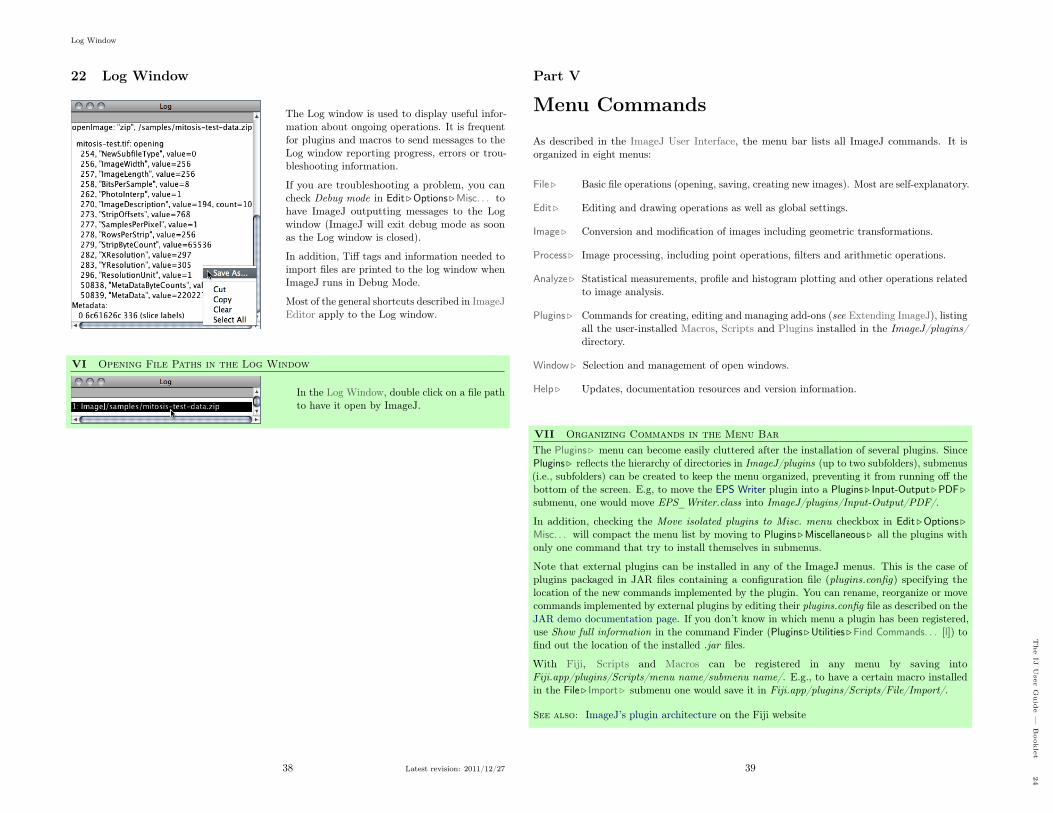
Log Window

22 Log Window

The Log window is used to display useful infor-mation about ongoing operations. It is frequentfor plugins and macros to send messages to theLog window reporting progress, errors or trou-bleshooting information.

If you are troubleshooting a problem, you cancheck Debug mode in Edit .Options .Misc. . . tohave ImageJ outputting messages to the Logwindow (ImageJ will exit debug mode as soonas the Log window is closed).

In addition, Tiff tags and information needed toimport files are printed to the log window whenImageJ runs in Debug Mode.

Most of the general shortcuts described in ImageJEditor apply to the Log window.

VI Opening File Paths in the Log Window

In the Log Window, double click on a file pathto have it open by ImageJ.


Part V

Menu Commands

As described in the ImageJ User Interface, the menu bar lists all ImageJ commands. It isorganized in eight menus:

File . Basic file operations (opening, saving, creating new images). Most are self-explanatory.

Edit . Editing and drawing operations as well as global settings.

Image . Conversion and modification of images including geometric transformations.

Process . Image processing, including point operations, filters and arithmetic operations.

Analyze . Statistical measurements, profile and histogram plotting and other operations relatedto image analysis.

Plugins . Commands for creating, editing and managing add-ons (see Extending ImageJ), listingall the user-installed Macros, Scripts and Plugins installed in the ImageJ/plugins/directory.

Window . Selection and management of open windows.

Help . Updates, documentation resources and version information.

VII Organizing Commands in the Menu Bar

The Plugins . menu can become easily cluttered after the installation of several plugins. SincePlugins . reflects the hierarchy of directories in ImageJ/plugins (up to two subfolders), submenus(i.e., subfolders) can be created to keep the menu organized, preventing it from running off thebottom of the screen. E.g, to move the EPS Writer plugin into a Plugins . Input-Output .PDF .submenu, one would move EPS_Writer.class into ImageJ/plugins/Input-Output/PDF/.

In addition, checking the Move isolated plugins to Misc. menu checkbox in Edit .Options .Misc. . . will compact the menu list by moving to Plugins .Miscellaneous . all the plugins withonly one command that try to install themselves in submenus.

Note that external plugins can be installed in any of the ImageJ menus. This is the case ofplugins packaged in JAR files containing a configuration file (plugins.config) specifying thelocation of the new commands implemented by the plugin. You can rename, reorganize or movecommands implemented by external plugins by editing their plugins.config file as described on theJAR demo documentation page. If you don’t know in which menu a plugin has been registered,use Show full information in the command Finder (Plugins .Utilities .Find Commands. . . [l]) tofind out the location of the installed .jar files.

With Fiji, Scripts and Macros can be registered in any menu by saving intoFiji.app/plugins/Scripts/menu name/submenu name/. E.g., to have a certain macro installedin the File . Import . submenu one would save it in Fiji.app/plugins/Scripts/File/Import/.

See also: ImageJ’s plugin architecture on the Fiji website

39

The

IJUser

Guid

e—

Bookle

t24

File .

23 File .

23.1 New .

Contains commands for creating new images, stacks, hyperstacks or text windows.

See also: Plugins .New .

23.1.1 Image. . . [n]

Creates a new image window or stack. A dialog box allowsyou to specify the image title, type, dimensions and initialcontent.

Name is the title that will be used for the Window. Typeis the image type: 8–bit grayscale, 16–bit grayscale (un-signed), 32–bit (float) grayscale or RGB color. Fill With(White, Black or Ramp) specifies how the image is initial-ized. Width and Height specify the image dimensions inpixels. Set Slices to a value greater than one to create astack.

See also: Image .Hyperstacks .New Hyperstack. . . , Image Types and Formats

23.1.2 Hyperstack. . .

Alias for the Image .Hyperstacks .New Hyperstack. . . command.

23.1.3 Text Window [N]

Creates a new text window with the title ‘Untitled.txt’.

See also: Plugins .New .Text Window. . . , Macro, Table. . .

23.1.4 Internal Clipboard

Opens the contents of the internal ImageJ clipboard.

See also: Edit .Copy [c], Cut [x], Paste Control. . .

23.1.5 System Clipboard [V]

Opens the contents of the operating system clipboard.

See also: Edit .Copy to System, Cut [x], Paste Control. . .


File . Open. . .

23.2 Open. . .

Opens an image and displays it in a separate window. Image files must be in TIFF, GIF, JPEG,DICOM, BMP, PGM or FITS format, or in a format supported by a reader plugin. Also opens:

– ImageJ and NIH Image lookup tables (.lut extension).

– Tables (in tab-delimited text format) (.xls or .csv extension, see Results Table)

– Selections (.roi or .zip extension)

– Text files (.txt, .ijm, .js and .java extensions)

– . . .

See also: File . Import . , Image Types and Formats, Virtual Stacks, VIII Opening Files: File .Open, File . Import and Drag & Drop

VIII Opening Files: File .Open, File . Import and Drag & Drop

While the File .Open. . . command opens formats natively supported by ImageJ (images andnon-images files), the File . Import . submenu provides access to plugins for additional file types(e.g., reading ‘raw’ files, images in ASCII format or loading images over the network). Most ofImageJ’s Input/Output plugins are installed on this submenu.

Note that almost every format known to ImageJ can be opened by dragging and dropping thefile into the ImageJ Window. E.g., in the illustration below a remote macro file is opened bydragging its URL directly from a Web browser.

23.3 Open Next [O]

Closes the current image and opens the next image (if any) in its directory. Holding Alt opensthe previous image (if any) in its directory.

23.4 Open Samples .

Opens example images hosted on the ImageJ Web site. These sample images are useful forcreating, testing and debugging macros since routines can be applied to the same image,regardless of where the macro is run. Among all, probably the most used is blobs.gif : OpenSamples .Blobs (25K) [B].

Sample images can be downloaded from http://imagej.nih.gov/ij/images/ or, in bulk, fromhttp://imagej.nih.gov/ij/download/sample-images.zip. The ‘AutoRun’ macro in the Startup-Macros.txt file can be used to change the default path of sample images, allowing a completeoff-line usage of the File .Open Samples . submenu:


The

IJUser

Guid

e—

Bookle

t25

File . Open Recent .

(5) Setting File .Open Samples . for Offline Usage1 /* This macro calls the Prefs.setImageURL () method to change the default path

of Sample Images (http :// imagej.nih.gov/ij/images /) to a local subfolder ofImageJ 's directory named "samples ". Note that Fiji provides this feature bydefault.

2 */3

4 macro "AutoRun" {5 dir= getDirectory("imagej") + "samples";6 i f (File.exists(dir)) {7 dir= replace(dir , " ", "%20");8 i f (startsWith(getInfo("os.name"), "Windows"))9 dir= "/"+ replace(dir , File.separator , "/");

10 call("ij.Prefs.setImagesURL", "file ://"+ dir +"/");11 }

23.5 Open Recent .

The submenu shows a list of the 15 recently opened files. Click on a filename to open it.

23.6 Import .

This submenu lists the installed image reader plugins.

See also: Non–native Formats, Acquisition plugins, Input/Output plugins, VirtualStackFrom-List macro, VIII Opening Files: File .Open, File . Import and Drag & Drop

23.6.1 Image Sequence. . .Improvedin IJ 1.45mImprovedin IJ 1.45m

Opens a series of images in a chosen folder as a stack. Imagesmay have different dimensions and can be of any formatsupported by ImageJ (see Image Types and Formats andHandleExtraFileTypes plugin). Invisible files, Thumbs.db orRoiSet.zip files created by the ROI Manager. . . are ignored.

Information – width×height×depth (size) – of the stack tobe created is displayed at the bottom of the dialog.

Number of Images Specifies how many images to open.

Starting Image If set to n, import will start with the nth

image in the folder.

Increment If set to ‘2’ every other image will be opened,if set to ‘3’ to every third image will be opened, etc.

File Name Contains Enter a string into this field and ImageJ will only open files whosename contains that string.

Enter Pattern Regular expressions (regex) can be typed here for advanced filtering (cf. Basicsyntax of regular-expressions).

Scale Images Setting a value less than 100% will reduce memory requirements. E.g., entering50 reduces the amount of memory needed to open a stack by 75%.


File . Import .

Convert to RGB Allows a mixture of RGB and grayscale images to be opened by convertingall the sequence to RGB. Note that if this option is unchecked and the first importedimage is 8–bit then all the remaining images in the sequence will be converted to 8–bit.Checking this option, circumvents this issue.

Sort Names Numerically When checked, the stack will be opened in numeric file nameorder (e.g., ‘name1.tif’, ‘name2.tif’, ‘name10.tif’) instead of alphanumeric order (e.g.,‘name1.tif’, ‘name10.tif’, ‘name2.tif’). DICOM files in the same series (tag#0020, 0011)are always sorted by the image number (tag#0020,0013). The List Stack Tags macro,part of the ListDicomTags macro set, lists the values of the image number and imageseries tags.

Use Virtual Stack When checked, images are opened as a read-only virtual (disk-resident)stack using a version of the Virtual Stack Opener plugin. This allows image sequencestoo big to fit in RAM to be opened, but access time is slower and changes are lost whenswitching to a different image in the stack (cf. Virtual Stacks).

Help Opens http://imagej.nih.gov/ij/docs/menus/file.html#seq1.

See also: OpenSeriesUsingFilter macro

Regular-expressions basic syntax summary. For more information on regex filtering see http://download.oracle.com/javase/tutorial/essential/regex/.

Regex Syntax (Character Classes) Example Meaning

[ ] Delimit the set of characters to match [aA] Either lower or upper case A- Character ranges [0-9] Any digit (from 0 through 9). Any character [0-9]. A digit plus any other character* Zero or more of the preceding item .* Any character sequence? Zero or one of the preceding item [0-9]? An optional digit+ One or more of the preceding item [0-9]+ At least a digit^ Negation [^0-9] Any character that is not a digit&& AND (Intersection) [0-9&&[^3]] A digit that is not 3| OR (Alternation) [0-9]|[a-zA-Z] A digit or lower or upper case letter

IX Reducing Memory Requirements When Importing Images

Since ImageJ 1.44d, the File . Import . . Image Sequence. . . command no longer features theConvert to 8-bit Grayscale checkbox. This option was used to reduce memory requirements butused different scaling for each imported image.

As a replacement, use the Use virtual stack option and then convert to 8–bit using File .Type .8–bit. Memory requirements can also be reduced by using the Scale Images (%) option.

See also: Edit .Options .Memory & Threads. . .


The

IJUser

Guid

e—

Bookle

t26

File . Import .

23.6.2 Raw. . .

Use this command to import images thatare not in a file format directly supportedby ImageJ. You will need to know certaininformation about the layout of the imagefile, including the size of the image, and theoffset to the beginning of the image data.

Interleaved RGB images have pixels storedcontiguously (rgbrgbrgb. . . ) in a single im-age plane. Planar RGB images have the red,green and blue image data stored in sepa-rate 8–bit sample planes. ImageJ saves RGBimages (both TIFF and raw) in interleavedformat.

Image Type There are fourteen choices depicted above. 16–bit signed integer images are convertedto unsigned by adding 32,768. 1–bit Bitmap images are converted to 8–bit.

Image Width The number of pixel in each row of image data.

Image Height The number of rows in the image.

Offset to First Image The number of bytes in the file before the first byte of image data.

Number of Images The number of images stored in the file. If this value is greater than theactual number of images the resulting stack will get truncated to the actual size.

Gap Between Images The number of bytes from the end of one image to the beginning ofthe next. Set this value to width×height×bytes-per-pixel×n to skip n images for eachimage read.

White is Zero Should be checked if black pixels are represented using numbers that are lessthan the numbers used for white pixels. If your images look like photographic negatives,changing this field should fix the problem.

Little-Endian Byte Order Probably needs to be checked when importing 16–bit or 32–bitgrayscale images from little-endian machines such as Intel based PCs.

Open All Files in Folder If checked, ImageJ will import all the images in the folder as astack. The images must all be the same size and type.

Use Virtual Stack Images are imported as virtual stacks.

Help Opens http://imagej.nih.gov/ij/docs/menus/file.html#raw.

See also: Image Types and Formats

23.6.3 LUT. . .

Opens an ImageJ or NIH Image lookup table, or a raw lookup table. The raw LUT file must be768 bytes long and contain 256 reds, 256 blues and 256 greens. If no image is open, a 256×32ramp image is created to display the LUT. Note that lookup tables with file names ending in.lut can also be opened using File .Open. . . or drag and drop.


File . Import .

23.6.4 Text Image. . .

Opens a tab-delimited text file as a 32–bit real image (see Text Images). The image’s widthand height are determined by scanning the file and counting the number of words and lines.For text files with integer values no larger than 255, use Image .Type . 8–bit to convert to 8–bit.Before converting, disable Scale When Converting in Edit .Options .Conversions. . . to preventthe image from being scaled to 0–255.

See also: OpenTextImagesAsStack macro, Save As .Text Image. . .

23.6.5 Text File. . .

Opens a text file. Note that text files can also be opened using File .Open. . . or drag and drop.

23.6.6 URL. . .

Downloads and displays known formats toImageJ specified by a URL. Other URLs end-ing with ‘/’ or ‘.html’ are opened in the user’sdefault browser. The Input URL is savedin the ImageJ preferences file and retrievedacross IJ restarts.

With IJ 1.44g and later, it is possible to open zip archives, using a URL, that contain multipleDICOM images. Some example URLs are:

– http://imagej.nih.gov/ij/images/ct.dcm

– file:///Macintosh HD/images/Nanoprobes.tif

– file:///D:\images\neuron.tif

– http://imagej.nih.gov/ij/ (opens the ImageJ website)

23.6.7 Results. . .

Opens an ImageJ table, or any tab or comma-delimited text file (see Results Table). Note that.csv and .xls files can also be opened by drag and drop.

23.6.8 Stack From List. . . Improvedin IJ 1.45mImprovedin IJ 1.45m

Opens a stack, or virtual stack, from a text file or URL containing a list of image file paths [9].The images can be in different folders but they must all be the same size and type. The VirtualStack From List macro demonstrates how to generate a list of images and then use that list toopen the images as a virtual stack. The OpenStackUsingURLs macro demonstrates how to howto open an image series from a remote server.

23.6.9 TIFF Virtual Stack. . .

Opens a TIFF file as virtual stack (see Virtual Stacks and III Opening Virtual Stacks by Drag& Drop).


The

IJUser

Guid

e—

Bookle

t27

File . Close [w]

23.6.10 AVI. . .

Uses a built in version of the AVI reader plugin to open an AVI file(JPEG or PNG compressed, or uncompressed) as a stack or virtualstack (one slice per video frame). AVI files can also be opened usingFile .Open. . . or drag and drop but macros must use this commandto gain access to the dialog box options.

Please note that ImageJ only supports a restricted number of AVIformats (cf. plugin source code).

Since version 1.41b an improved version of the AVI reader [10] retrieves animation speed fromimage frame rate, adds support for YUV formats, the ability to specify the starting and endingframe, an option to convert to 8–bit grayscale, an option to open the movie as a virtual stack,along with many bug fixes.

23.7 Close [w]

Closes the active image.

23.8 Close All

Closes all open images. An alert is displayed ifthere are unsaved changes.

23.9 Save [s]

Saves the active image in TIFF format, the ‘default’ format of ImageJ (cf. II Image Types:Lossy Compression and Metadata). To save only a selected area, create a rectangular selectionand use the Image .Duplicate. . . [D] command. Note that Save [s] and File . Save As .Tiff. . . areredundant commands.

23.10 Save As .

Use this submenu to save the active image in TIFF, GIF, JPEG, or ‘raw’ format. Can also beused to save measurement results, lookup tables, selections, and selection XY coordinates.

23.10.1 Tiff. . .

Saves the active image or stack in TIFF format in redundancy with File .Save [s]. TIFF is theonly format (other than ‘raw’) that supports all ImageJ data types (8–bit, 16–bit, 32–bit floatand RGB) and the only format that saves spatial and density calibration. In addition, withIJ 1.43 and later, selections and overlays are also saved in the TIFF header.

By default, 16–bit and 32–bit images are saved using big-endian byte order. Check Save TIFFand Raw in Intel Byte Order in the Edit .Options . Input/Output. . . dialog box to save usinglittle-endian byte order.

See also: Native Formats, II Image Types: Lossy Compression and Metadata, X Warning onJPEG compression


File . Save As .

23.10.2 Gif. . .

Saves the active image in GIF format. RGB images must first be converted to 8–bit color usingusing Image .Type . 8–bit Color. The value to be used as the transparent index (0–255) can beset in the Edit .Options . Input/Output. . . dialog box. Stacks are saved as animated GIFs. UseImage . Stacks .Tools .Animation Options. . . [Alt /] (or right-click on the on the play/pause iconthat precedes the stack slider) to set the frame rate.

23.10.3 Jpeg. . .

Saves the active image in JPEG format. Edit JPEG Quality Edit .Options . Input/Output. . .dialog box to specify the JPEG compression level (0–100). This value is shown on the title ofthe save dialog prompt. Lower values produce smaller files but poorer quality. Larger valuesproduce larger files but better quality. Color sub-sampling is disabled when the value is set to100, reducing the likelihood of color artifacts. By default, the DPI in the JPEG header is setto 72. For a higher value, use a unit of inch in the Analyze .Set Scale. . . dialog. E.g., settingDistance in Pixels to 300, Known Distance to 1 and Unit of Length to ‘inch’ will set the DPI to300.

Since IJ 1.43 and later, overlays are embedded when saving in Jpeg format (cf. Flatten [F]).

See also: II Image Types: Lossy Compression and Metadata, X Warning on JPEG compression

X Warning on JPEG compressionThe JPEG format uses lossy compression that can result in artifacts. You should never usedthis format on images to be segmented or measured.

23.10.4 Text Image. . .

Saves the active image as a spreadsheet compatible tab-delimited text file. For calibratedimages and floating-point images, the Decimal Places field in Analyze .Set Measurements. . .determines the number of digits to the right of the decimal point. For RGB images, eachpixel is converted to grayscale using the formula gray = (red+ green+ blue)/3 or the formulagray = 0.299× red+ 0.587× green+ 0.114× blue if Weighted RGB to Grayscale Conversion ischecked in Edit .Options .Conversions. . .

See also: Import .Text Image. . .

23.10.5 Zip. . .

Saves the active image or stack as a TIFF file inside a compressed ZIP archive.


The

IJUser

Guid

e—

Bookle

t28

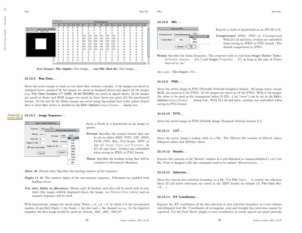
File . Save As .

Text Images: File . Import .Text Image. . . and File .Save As .Text Image. . .

23.10.6 Raw Data. . .

Saves the active image or stack as raw pixel data without a header. 8–bit images are saved asunsigned bytes, unsigned 16–bit images are saved as unsigned shorts and signed 16–bit images(e.g., File .Open Samples .CT (420K, 16–bit DICOM)) are saved as signed shorts. 32–bit imagesare saved as floats and RGB images are saved in three bytes per pixel (24–bit interleaved)format. 16–bit and 32–bit (float) images are saved using big-endian byte order unless ExportRaw in Intel Byte Order is checked in the Edit .Options . Input/Output. . . dialog box.

23.10.7 Image Sequence. . .Improvedin IJ 1.45mImprovedin IJ 1.45m

Saves a Stack or a hyperstack as an image se-quence.

Format Specifies the output format that canbe set to either BMP, FITS, GIF, JPEG,PGM, PNG, Raw, Text Image, TIFF, orZip (cf. Image Types and Formats). InIJ 1.44 and later, overlays are embeddedwhen saving in JPEG or PNG format.

Name Specifies the leading string that will becommon to all numeric filenames.

Start At (Stacks only) Specifies the starting number of the sequence.

Digits (1–8) The number digits of the incremental sequence. Filenames are padded withleading zeroes.

Use slice labels as filenames (Stacks only) If checked, each slice will be saved with its ownlabel (the image subtitle displayed above the image, see Remove Slice Labels) and nonumeric sequence will be used.

With hyperstacks, images are saved using ‘Name_t d_z d_c d ’ in which d is the incrementalnumber of specified Digits; t, the frame; z, the slice and c, the channel, so e.g., for the depictedsnapshot the first image would be saved as ‘mitosis_t001_z001_c001.tif’.


File . Save As .

23.10.8 AVI. . .

Exports a stack or hyperstack as an AVI file [10].

Compression JPEG, PNG or Uncompressed.With IJ 1.44 and later, overlays are embeddedwhen saving in JPEG or PNG format. Thedefault compression is JPEG.

Frame Specifies the frame frequency. The proposed value is read from Image . Stacks .Tools .Animation Options. . . [Alt /] and Image .Properties. . . [P], as long as the unit of FrameInterval is ‘sec’.

See also: File . Import .AVI. . .

23.10.9 PNG. . .

Saves the active image in PNG (Portable Network Graphics) format. All image types, exceptRGB, are saved as 8–bit PNGs. 16–bit images are saved as 16–bit PNGs. With 8–bit images,the value to be used as the transparent index (0–255, -1 for “none”) can be set in the Edit .Options . Input/Output. . . dialog box. With IJ 1.44 and later, overlays are embedded whensaving in PNG format.

23.10.10 FITS. . .

Saves the active image in FITS (Flexible Image Transport System) format [11].

23.10.11 LUT. . .

Saves the active image’s lookup table to a file. The 768 byte file consists of 256 red values,256 green values and 256 blue values.

23.10.12 Results. . .

Exports the contents of the ‘Results’ window as a tab-delimited or comma-delimited (.csv) textfile. Prior to ImageJ 1.44b this command used to be named ‘Measurements. . . ’.

23.10.13 Selection. . .

Saves the current area selection boundary to a file. Use File .Open. . . to restore the selection.Since IJ 1.43 active selections are saved in the TIFF header by default (cf. File .Save As .Tiff. . . ).

23.10.14 XY Coordinates. . .

Exports the XY coordinates of the line selection or area selection boundary as a two column,tab-delimited text file. Coordinates of rectangular, oval and straight line selections cannot beexported. Use the Path Writer plugin to save coordinates at evenly spaced one pixel intervals.


The

IJUser

Guid

e—

Bookle

t29

File . Revert [r]

23.11 Revert [r]

Reloads the active image, stack or hyperstack from disk, reverting it to its last saved state. It isactually a shortcut for closing the window without saving, and then reopening it.

See also: Undo and Redo

23.12 Page Setup. . .

The Page Setup dialog allows you to control the size of printedoutput, plus other printing options:

Scale Values less than 100% reduce the size of printed images andvalues greater than 100% increase the size. 100% correspondsto 72 pixels per inch (ppi), about the unzoomed screen sizeof the image. The size of the printed image is determinedby the Scale value and the width and height of the image inpixels. Spatial calibration is ignored.

Draw border If checked, ImageJ will print a one pixel wide black border around the image.

Center on page If checked, the image will be printed in the center of the page instead of inthe upper left corner.

Print title If checked, the title of the image will be printed at the top of the page.

Selection only If checked, current selection will be printed instead of the entire image.

Rotate 90 ◦ If checked, the image will be rotated 90◦ to the left before being printed.

Print actual size Considers the DPI information in the image header (typically 72, cf.Jpeg. . . ). For a higher value, use a unit of inch in the Analyze .Set Scale. . . dialog.E.g., setting Distance in Pixels to 300, Known Distance to 1 and Unit of Length to ‘inch’will set the DPI to 300.

23.13 Print. . . [p]

Prints the active image. The size of the printed image will normally be slightly less its sizeon the screen (unzoomed). Use the Page Setup. . . dialog to increase of decrease the size ofprinted images. Images larger than the page are scaled to fit. With IJ 1.44 and later, overlaysare embedded when printing.

23.14 Quit

Prompts you to save all unsaved images and then exits. You can also exit ImageJ by clicking onthe close button in its window’s title bar.


Edit .

24 Edit .

24.1 Undo [z]

Described in Undo and Redo.

24.2 Cut [x]

Copies the contents of the current image selection to the internal clipboard and fills it with thecurrent background color.

See also: Edit .Copy to System, Paste Control. . .

24.3 Copy [c]

Copies the contents of the current image selection to the internal clipboard. If there is noselection, copies the entire active image. The amount of image data copied is shown in thestatus bar.

See also: File . Internal Clipboard, Paste Control. . .

24.4 Copy to System

Copies the contents of the current image selection to the system clipboard.

See also: File .New . System Clipboard [V], Copy [c], Paste Control. . .

24.5 Paste [v]

Inserts the contents of the internal clipboard (or from the system clipboard if the internalclipboard is empty) into the active image. The pasted image is automatically selected, allowingit to be dragged with the mouse. Click outside the selection to terminate the paste. SelectEdit .Undo [z] to abort the paste operation.

See also: Paste Control. . .

24.6 Paste Control. . .

After pasting, use the Paste Control pop-up menu to con-trol how the image currently being pasted is transferredto the destination image.

Except for Blend and Transparent, the Paste Controltransfer modes are the same as those listed in the descrip-tion of Process . Image Calculator. . . . The Blend modeis the same as the Image Calculator Average mode. InTransparent mode, white/black pixels are transparentand all other pixels are copied unchanged.

See also: Image .Overlay . Add Image. . .


The

IJUser

Guid

e—

Bookle

t30

Edit . Clear

24.7 Clear

Erases the contents of the selection to the current background color. Backspace and Del keysare shortcuts to this command. With stacks, a dialog is displayed offering the option to clearthe selection in all stack images. Clear by pressing Backspace to avoid this dialog.

See also: Clear Outside, Fill [f], Color Picker

24.8 Clear Outside

Erases the area outside the current image selection to the background color.

See also: Clear, Fill [f], Color Picker

24.9 Fill [f]

Fills the current selection with the current foreground color. With stacks, a dialog is displayedoffering the option to fill the selection in all stack images. Fill the selection by pressing F toavoid this dialog.

See also: Clear, Draw [d], Color Picker

24.10 Draw [d]

Outlines the current selection using the current foreground color and line width. The foregroundand background colors can also be set using the Edit .Options .Colors. . . command. Use theEdit .Options . Line Width. . . command, or double click on the line tool, to change the linewidth.

With stacks, a dialog is displayed offering the option to draw the selection in all stack images.Draw the selection by pressing D to avoid this dialog.

See also: Analyze . Label, Color Picker, XVII Embedding Color Annotations in GrayscaleImages, XI Drawing Lines Wider Than One–Pixel

XI Drawing Lines Wider Than One–PixelIf the line width is an even number, the selection boundary is at the center of the line. If theline width is odd (1, 3, . . . ), the center of the line drawn is displaced from the selection edgeby 1/2 pixel to the bottom right. Thus the line center (the line in case of linewidth = 1) isinside the selection at the top and left borders, but outside at the bottom and right borders.Rectangular selections (but not polygonal selections or traced selections that happen to berectangular) are an exception to this rule: For rectangular selections, one–pixel wide outlinesare always drawn inside the rectangle. Thicker lines are drawn as for the other selection types.


Edit . Invert [I]

24.11 Invert [I]

Creates a reversed image, similar to a photographic negative, of the entire image or selection.

See also: Image . Lookup Tables . Invert LUT

24.12 Selection .

Original FitSpline

FitCircle

FitEllipse

ConvexHull

MakeInverse

CreateMask

Area toLine

MakeBand. . .

ToBounding

Box

ROI manipulations using the Edit . Selection . submenu commands.

24.12.1 Select All [a]

Creates a rectangular selection that is the same size as the image.

24.12.2 Select None [A]

Deactivates the selection in the active image.

24.12.3 Restore Selection [E]

Restores the previous selection to its original position. A selection is saved when you:

– Delete the selection by clicking outside of it

– Draw a new selection

– De-activate the image containing the selection

– Close the image containing the selection

– Use a command that deletes or modifies the selection

See also: Analyze .Tools .ROI Manager. . .

XII Transferring Selections Between ImagesYou can transfer a selection from one image to another by activating the image with theselection, activating the destination image, then pressing Shift E (the keyboard shortcut forEdit . Selection .Restore Selection [E]).


The

IJUser

Guid

e—

Bookle

t31

Edit . Selection .

24.12.4 Fit Spline

Fits a cubic spline curve to a polygon or polyline selection (see ROI manipulations).

24.12.5 Fit Circle

Fits a circle to a multipoint (with at leas 3 points) or area selection [12] (see ROI manipulations).Composite selections are not supported. With open shapes (lines and points), the fittingalgorithm (Newton-based Pratt fit) described in Pratt V, “Direct least-squares fitting of algebraicsurfaces”, Computer Graphics, Vol. 21, pp 145–152 (1987) is used. With closed shapes, thecommand creates a circle with the same area and centroid of the selection.

24.12.6 Fit Ellipse

Replaces an area selection with the best fit ellipse (see ROI manipulations). The ellipse will havethe same area, orientation and centroid as the original selection. The same fitting algorithm isused to measure the major and minor axis lengths and angle when Fit Ellipse is selected inAnalyze . Set Measurements. . .

See also: DrawEllipse macro

24.12.7 Convex Hull

Replaces a polygon of freehand selection with its convex hull (see ROI manipulations), determinedby the gift wrap algorithm. The convex hull can be thought of as a rubber band wrapped tightlyaround the points that define the selection.

See also: Fit Ellipse, ConvexitySolidarity macro, Convex_Hull_Plus plugin

24.12.8 Make Inverse

Creates an inverse selection (see ROI manipulations). What is ‘inside’ the selection will be‘outside’, and vice versa.

24.12.9 Create Mask

Creates a new 8–bit image called ‘Mask’ whose pixels have a value of 255 inside the selectionand 0 outside (see ROI manipulations). By default, this image has an inverting LUT, so blackis 255 and white is 0 unless Black Background in Process .Binary .Options. . . is checked.

See also: Process .Binary .Convert to Mask, XX Creating Binary Masks, XXI InterpretingBinary Images

24.12.10 Create Selection

Creates a selection from a thresholded image or a binary mask [13].


Edit . Selection .

24.12.11 Properties. . . [y] Improvedin IJ 1.45mImprovedin IJ 1.45m

Opens a dialog box that allows the user to assign a contourcolor (Stroke Color) and a contour width (Width) to theactive selection or a filling color. Note that selections can beeither filled or contoured, but not both.

The nine default selection colors (black, blue, cyan, green,magenta, orange, red, white, yellow) can be typed textually.Any other color must be typed using hex notation (see XIXHexadecimal Color Values).

With text selections (see Text Tool), it is also possible to specify the font size and text alignment.

Note that while this command can only be applied to the active selection, the ROI Manager’sProperties. . . command (Analyze .Tools .ROI Manager. . . ) can be applied to multiple ROIs.

See also: Selections, Image .Overlay .Add Selection. . . [b]

24.12.12 Rotate. . .

Rotates the selection by the specified number of degrees (negativenumber indicate counter-clockwise rotation). This command runsthe RotateSelection macro in ij.jar.

See also: FlipSelection macro

24.12.13 Enlarge. . .

Grows an area selection by a specified number of pixels. Enter anegative value to shrink the selection. This command runs theEnlargeSelection macro in ij.jar. ShrinkSelection is a variationof this macro that does not shrink from the image edges.

XIII Converting Composite Selections

Enter zero in the Edit . Selection .Enlarge. . . dialog box to convert a composite selection into apolygon selection. Note, however, that the conversion may fail if the composite ROI is composedof more than one piece and/or contains internal holes.

24.12.14 Make Band. . . Improvedin IJ 1.45mImprovedin IJ 1.45m

Takes an area selection and creates a band with a thickness of thespecified number of pixels (see ROI manipulations). If you imagine theband as a doughnut shape, then the original selection corresponds tothe hole (i.e. the band is made by growing out the original selection).

See also: MakeSelectionBand, the macro that implemented thiscommand in previous IJ versions.


The

IJUser

Guid

e—

Bookle

t32

Edit . Selection .

24.12.15 Specify. . .

Opens a dialog that allows the user to define a rectangular or ellipticalselection. Width and Height are the dimensions of the selection. XCoordinate and Y Coordinate define the position of the selection.Check Oval to create an elliptical selection. If Centered is checked,the selection is positioned so X Coordinate and Y Coordinate definethe center of the selection, otherwise they define the upper left corner.

This command is also available through the ROI Manager More�drop-down menu (see Analyze .Tools .ROI Manager. . . ).

24.12.16 Straighten. . .

This command straightens a curved object in an image. The curved object must first be outlinedusing the segmented line tool. Use the Image .Adjust . Line Width. . . widget, opened by doubleclicking on the line tool icon, to adjust the width of the line selection. Check Spline Fit inthe Line Width widget to fit a cubic spline curve to the points that define the line. WithIJ 1.44k and later, it is not necessary to check the status of the Spline Fit checkbox since Edit .Selection . Straighten. . . will assess if the line has already been prepared for straightening by arun("Fit Spline", "straighten") call.

Drag the points along the line selection to reposition them. Alt-click on a point to delete it.Shift-click on a point to duplicate it. Press Shift E (Edit .Selection .Restore Selection [E]) torestore accidentally deleted lines.

Straighten. . . also works with straight line selections. In this case, the object defined by the lineselection is rotated to be horizontal.

Edit . Selection . Straighten. . .

24.12.17 To Bounding Box

Converts a non-rectangular selection to the smallest rectangle that completely contains it.

24.12.18 Line to Area

Converts a line selection to an area (traced) ROI. Straight lines must be wider than one pixel.


Edit . Options .

24.12.19 Area to Line New inIJ 1.45mNew inIJ 1.45m

Converts a non-composite area selection to its enclosing outline (see ROI manipulations). Theobtained line will have the width specified in the Image .Adjust . Line Width. . . widget. Notethat by design Area to Line does not create closed paths. E.g., the converted outline of arectangular selection will be composed of only three segments, with the first and fourth cornerpoints of the rectangle being disconnected.

See also: Composite Selections, Line to Area

24.12.20 Add to Manager [t]

Adds the current selection to the ROI Manager (Analyze .Tools .ROI Manager. . . ). If there isno selection the ROI Manager is open.

24.13 Options .

Use commands in this submenu to change various ImageJ user preference settings.

24.13.1 Line Width. . .

Displays a dialog box that allows to change the line width (in pixels)of line selections (see Line Selection Tools) and concomitantly thelines generated by the Edit .Draw [d] command. This legacy commandhas been superseded by the Image .Adjust . Line Width. . . widget,but required since the later is not recordable (see Plugins .Macros .Record. . . ).

24.13.2 Input/Output. . .

JPEG quality (0–100) Specifies the compressionlevel used by File . Save As . Jpeg. . . Requesting ahigher degree of compression (a lower value) willresult in smaller files, but poorer image quality.Note that lossy JPEG compression creates seriousartifacts, see II Image Types: Lossy Compressionand Metadata.

GIF and PNG transparent index Specifies thetransparent color used for images saved in GIFand PNG formats. Use -1 for “none”. Note thatPNG and GIF transparency only works with 8–bitimages.

File extension for tables Sets the default extension to be used when saving tables (seeResults Table). Files with .txt and .xls extensions are saved in tab-delimited format andfiles with .csv extensions are saved in comma-delimited format.


The

IJUser

Guid

e—

Bookle

t33

Edit . Options .

Use JFileChooser to open/save Enables versions of File .Open and File . Save As that usethe Java JFileChooser instead of the native OS file open and save dialogs. The mainadvantage of JFileChooser is the ability to open multiple files by shift-clicking to selectmultiple contiguous files and control-clicking to select more than one individual file. Onthe other hand, it is slower, uses more memory, and does not behave like the file open andsave dialogs used in other applications.

Save TIFF and raw in intel byte order Specifies the byte order used when saving 16–bitand 32–bit images using File . Save As .Raw Data. . . , or File . Save As . Image Sequence. . .when Raw is chosen as the format. Check this option to export images using the order usedby Intel ×86 based processors (little-endian). This Wikipedia article has more information.

Results Table Options Specifies if column headers and row numbers should be saved orcopied from ImageJ tables such as the Results and Summarize windows (see ResultsTable).

24.13.3 Fonts. . .

Opens a small widget with three pop-up menus for specifying the type face, size, style andantialiasing (Smooth checkbox) of the font used by the Text Tool and Image . Stacks . Label. . .It is also possible to adjust the horizontal text alignment using the style drop-down menu: Left(the default), Right, or Centered. The widget is more easily opened by double clicking on theText Tool.

24.13.4 Profile Plot Options. . .

Use this dialog to control how plots generated by ImageJ are displayed (Image .Stacks .PlotZ-axis Profile. . . , Analyze .Plot Profile [k], Analyze .Calibrate. . . , Analyze .Tools .Curve Fitting. . . ,Multi Plot [Analyze .Tools .ROI Manager. . . ], etc.).

Plot Width and Plot Height Specify the length (in pixels)of the X-axis (Plot Width) and Y-axis (Plot Height).

Fixed y-axis Scale If checked, the Y-axis range is fixed andthe specifiedMinimum Y andMaximum Y values areused, otherwise, plots are scaled based on the minimumand maximum gray values.

Do not Save x–values If checked, ‘List ’, ‘Save. . . ’ and‘Copy . . . ’ buttons will appear in profile plot windows.

Auto–close If checked, profile plot windows will be automat-ically closed when ‘List’, ‘Save’ and ‘Copy’ are clickedon.

Vertical Profile If checked, row average plots of rectangular areas (or line selections widerthan 1 pixel) will be generated instead of the default column average plots. Note thatevoking Plot Profile [k] with Alt B will generate vertical profiles.


Edit . Options .

List values If checked, the list of values will be automatically opened. If Auto–close is alsochecked, the plot is closed and only the list of values remains open.

Interpolate line profiles If checked, profile values will be interpolated along the line selection

Draw grid lines If checked, gray grid lines will be drawn in the plot.

Help Opens http://imagej.nih.gov/ij/docs/menus/edit.html#plot-options.

24.13.5 Rounded Rect Tool. . . New inIJ 1.45mNew inIJ 1.45m

See Rounded Rectangular Selection Tool.

24.13.6 Arrow Tool. . .

See Arrow Tool.

24.13.7 Point Tool. . .

See Point Tool.

24.13.8 Wand Tool. . .

See Wand Tool.

24.13.9 Colors. . .

Displays a dialog box that allows you to set Foreground Color,Background Color and Selection Color.

See also: Color Picker, Image .Color .Color Picker. . . [K], PointTool

24.13.10 Appearance. . .

This dialog contains options that control how images are dis-played, an option to display better looking toolbar icons, andan option to set the menu font size.

Interpolate zoomed images Uses interpolation instead ofpixel replication when displaying zoomed images.

Open Images at 100% Newly open images are displayedusing 100% magnification (1 image pixel = 1 screen pixel).

Black Canvas Causes the image canvas (white by default) to be rendered in black. This isuseful when looking at X-ray images in order to avoid high contrasting intensities at theimage edges.


The

IJUser

Guid

e—

Bookle

t34

Edit . Options .

No image border Displays images without the default one pixel wide black border.

Use inverting lookup table Causes newly opened 8–bit images to have inverted pixel values,where white= 0 and black= 255. This is done by both inverting the pixel values andinverting the LUT. Use the Image . Lookup Tables . Invert LUT command to invert animage without changing the pixel values.

Double Buffer Selections Reduces flicker when working with complex selections but it alsoincreases memory usage and slows screen updates. It is not needed on Mac OSX, whichhas built in double buffering.

Antialiased tool icons Smooths and darken the tool icons in the ImageJ window. This optionis enabled by default on all operating systems. On Windows XP, enable Clear Typesub-pixel anti-aliasing to improve the quality of text in menus.

Menu font size Specifies the size of the ImageJ window menu font. Use a size of 0 (zero) touse Java’s default menu font size. Changing the font size requires the restarting of ImageJ.This option is ignored on Mac OSX.

Help Opens http://imagej.nih.gov/ij/docs/menus/edit.html#appearance.

24.13.11 Conversions. . .

Use this dialog to set options that control howimages are converted from one type to another.

Scale When Converting ImageJ will scale from min–max to 0–255 when converting from16–bit or 32–bit to 8–bit or to scale from min–max to 0–65535 when converting from32–bit to 16–bit. Note that Scale When Converting is always checked after ImageJ isrestarted.

Weighted RGB Conversions (0.30, 0.59, 0.11) When checked, the formula gray = 0.299×red+ 0.587× green+ 0.114× blue is used to convert RGB images to grayscale. If it is notchecked, the formula gray = (red+ green+ blue)/3 is used. The default weighting factors(0.299, 0.587, 0.114), which are based on human perception, are the ones used to convertfrom RGB to YUV, the color encoding system used for analog television. The weightingfactors can be modified using the setRGBWeights() macro function.

24.13.12 Memory & Threads. . .

Use this dialog to specify the maximum amount ofmemory available to ImageJ and the number of threadsused by filters when processing stacks. Java applications

such as ImageJ will only use the memory allocated tothem (typically 640MB) but this dialog allows the userto allocate more than the default.

Note that specifying more than 75% of real RAM could result in virtual RAM being used, whichmay cause ImageJ to become slow and unstable. Also note that this dialog cannot be used to


Edit . Options .

set the memory allocation if ImageJ is run from the command line or by double clicking onij.jar.

Maximum memory 64-bit OS and a 64–bit version of Java are required to use more than≈1700MB of memory. Windows users must be running a 64–bit version of Windows andmust install a 64–bit version of Java. Mac users must be running OS X 10.5 or later andmay need to use the Java Preferences utility (in /Applications/Utilities/Java) to selecta 64–bit version of Java. They may also need to switch to the ImageJ64 application.Linux users need to be running 64–bit versions of Linux and Java. The title of theMemory &Threads dialog box changes to Memory (64–bit) when ImageJ is running on aproperly configured 64–bit system.

Parallel threads for stacks Defaults to the number of available processors determines thenumber of parallel threads used by commands in the Process .Filters . and the Process .Math . submenus when processing stacks.

Keep multiple undo buffers If checked, the undo buffer will be preserved when switching New inIJ 1.45mNew inIJ 1.45m

images. Edit .Undo [z] remains restricted to the most recent operation, but is availablefor each opened image, as long as the buffer allows it. If Keep multiple undo buffers isunchecked, the undo buffer is reset every time the active (frontmost) image changes.

Run garbage collector on status bar click If checked, forces the Java garbage collector torun every time the user clicks on the ImageJ status bar, which may help to reclaim unusedmemory (cf. Status bar).

Help Opens http://imagej.nih.gov/ij/docs/menus/edit.html#memory.

See also: FAQ’s on the ImageJ Documentation Wiki

24.13.13 Proxy Settings. . . Improvedin IJ 1.45mImprovedin IJ 1.45m

Use this dialog to modify the proxy settings of the JavaVirtual Machine. This may be required for ImageJ to connectto the internet in certain machines running behind HTTPproxies. For example, proxy settings may be required toupdate ImageJ using the Help .Update ImageJ. . . commandor to open the images in the File .Open Samples . submenu.

To use the system proxy settings enable the Or use system proxy settings option (this will set thejava.net.useSystemProxies property to true). To configure your proxy settings manuallyspecify the address of the HTTP proxy in Proxy server and the port the proxy listens on(normally 8080) in Port. Settings will be saved in the ImageJ preferences file (IJ_Prefs.txt).

24.13.14 Compiler. . .

Displays a dialog box with options for the Plugins .Compile and Run. . . command.

Target Specifies the Java version of the class files. Pluginscompiled with a Target of 1.6 will not run on earlierversions of Java. A Target of 1.4 should be used tocreate plugins capable of running on all ImageJ versions.Target cannot be set higher than the version of JavaImageJ is currently running on.


The

IJUser

Guid

e—

Bookle

t35

Edit . Options .

Target Specifies the Java version of the class files created by Plugins .Compile and Run. . .Plugins compiled with a Target of 1.6 will not run on earlier version Java. A Target of 1.4should be used to create plugins capable of running on all versions ImageJ. Target cannotbe set higher than the version of Java ImageJ is currently running on.

Generate Debugging Info (javac -g) If checked, information needed by Java debuggerswill be included in the class files.

Help Opens http://imagej.nih.gov/ij/docs/menus/edit.html#compiler.

24.13.15 DICOM. . .Improvedin IJ 1.45mImprovedin IJ 1.45m

This dialog sets options related to the handling of DICOM images.Namely, if ImageJ should open DICOM images as 32–bit float, if voxeldepth should be calculated (based on the distance between the firstand last slice) and if coronal/transverse sections should be mirroredwhen using the Image . Stacks .Orthogonal Views [H] command. WithIJ 1.45, the DICOM reader applies the Rescale Slope value when Openas 32-bit float is enabled and tag 0028,1053 is not 1.0.

See also: Image Types and Formats

24.13.16 Misc. . .

Displays a dialog box containing miscellaneous options.

Divide by zero value Specifies the value used whenProcess . Image Calculator. . . detects a divide byzero while dividing one 32–bit real image by an-other. The default is infinity. In addition to nu-meric values, ‘infinity’ (positive or negative in-finity), ‘max’ (largest positive value) and ‘NaN’(Not-a-Number) can be entered as the Divide byzero value.

Use pointer cursor If checked, ImageJ will use an arrow cursor instead of the default cross-hair that is sometimes difficult to see on grayscale images in areas of medium brightness.This option can also be used to work around a bug on Windows where the text cursor issometimes used in place of the cross-hair.

Hide "Process Stack?" dialog If checked, ImageJ will suppress the dialog that asks ‘Processall xx slices?’ (only the current slice will be processed).

Require control / command key for shortcuts If checked, requires the Control key (Com-mand key on Macs) to be pressed when using keyboard shortcuts for menu commands.

Move isolated plugins to Misc. menu This option can reduce the size of the Plugins menu,preventing it from running off the bottom of the screen. When this option is enabled,plugins that attempt install themselves in a submenu with only one command are insteadinstalled in the Plugins .Miscellaneous submenu. An example of such a plugin is TurboReg,which normally creates a Plugins .TurboReg submenu that contains only one command.

Run single instance listener If checked, ImageJ will use sockets to prevent multiple in-stances from being launched. On Windows, this avoids the problem where another copy


Edit . Options .

of ImageJ starts each time an image is dragged and dropped on the ImageJ icon. It alsoprevents multiple instances when running ImageJ from the command line. Note that youmay get a security alert the first time ImageJ starts with this option enabled. ImageJdoes not require external socket access so it is okay to deny it access in the security alert.This option is set by default with new Windows installations.

Debug mode If checked, causes ImageJ to display debugging messages in the Log Window.Close the Log window to disable display of debugging messages.

Help Opens http://imagej.nih.gov/ij/docs/menus/edit.html#misc.


The

IJUser

Guid

e—

Bookle

t36

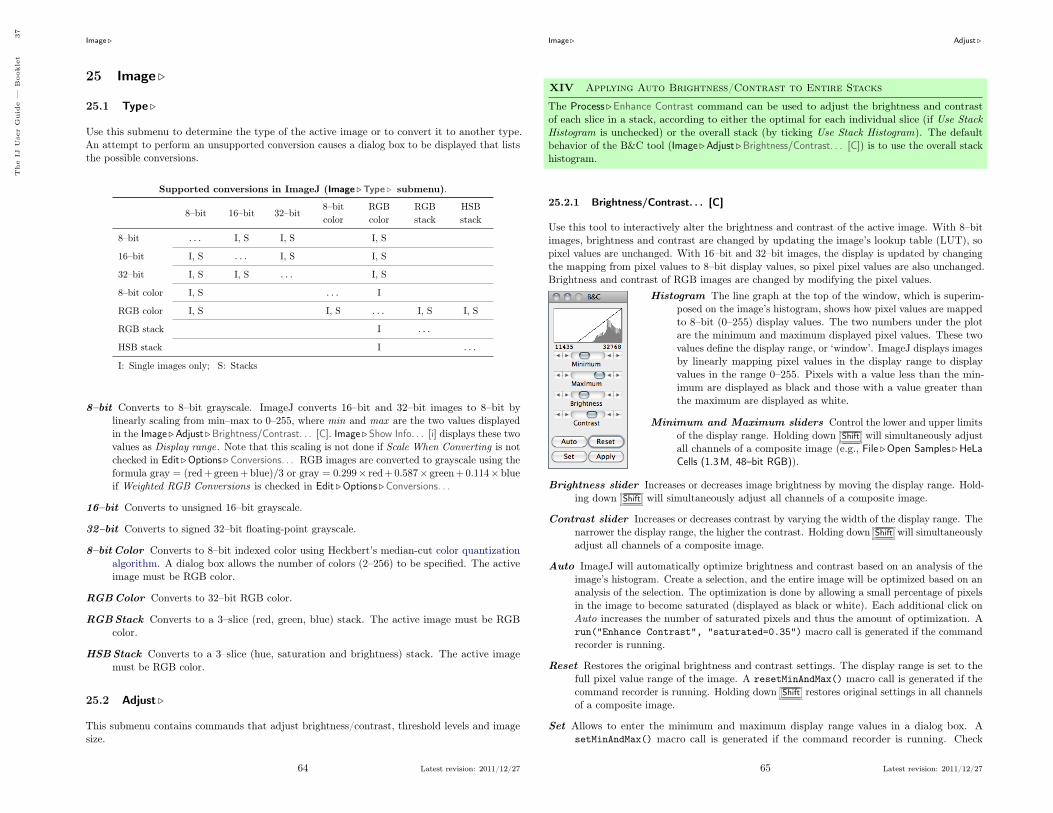
Image .

25 Image .

25.1 Type .

Use this submenu to determine the type of the active image or to convert it to another type.An attempt to perform an unsupported conversion causes a dialog box to be displayed that liststhe possible conversions.

Supported conversions in ImageJ (Image .Type . submenu).

8–bit 16–bit 32–bit8–bitcolor

RGBcolor

RGBstack

HSBstack

8–bit . . . I, S I, S I, S

16–bit I, S . . . I, S I, S

32–bit I, S I, S . . . I, S

8–bit color I, S . . . I

RGB color I, S I, S . . . I, S I, S

RGB stack I . . .

HSB stack I . . .

I: Single images only; S: Stacks

8–bit Converts to 8–bit grayscale. ImageJ converts 16–bit and 32–bit images to 8–bit bylinearly scaling from min–max to 0–255, where min and max are the two values displayedin the Image .Adjust .Brightness/Contrast. . . [C]. Image . Show Info. . . [i] displays these twovalues as Display range. Note that this scaling is not done if Scale When Converting is notchecked in Edit .Options .Conversions. . . RGB images are converted to grayscale using theformula gray = (red+ green+blue)/3 or gray = 0.299× red+0.587× green+0.114×blueif Weighted RGB Conversions is checked in Edit .Options .Conversions. . .

16–bit Converts to unsigned 16–bit grayscale.

32–bit Converts to signed 32–bit floating-point grayscale.

8–bit Color Converts to 8–bit indexed color using Heckbert’s median-cut color quantizationalgorithm. A dialog box allows the number of colors (2–256) to be specified. The activeimage must be RGB color.

RGBColor Converts to 32–bit RGB color.

RGBStack Converts to a 3–slice (red, green, blue) stack. The active image must be RGBcolor.

HSBStack Converts to a 3–slice (hue, saturation and brightness) stack. The active imagemust be RGB color.

25.2 Adjust .

This submenu contains commands that adjust brightness/contrast, threshold levels and imagesize.


Image . Adjust .

XIV Applying Auto Brightness/Contrast to Entire Stacks

The Process .Enhance Contrast command can be used to adjust the brightness and contrastof each slice in a stack, according to either the optimal for each individual slice (if Use StackHistogram is unchecked) or the overall stack (by ticking Use Stack Histogram). The defaultbehavior of the B&C tool (Image .Adjust .Brightness/Contrast. . . [C]) is to use the overall stackhistogram.

25.2.1 Brightness/Contrast. . . [C]

Use this tool to interactively alter the brightness and contrast of the active image. With 8–bitimages, brightness and contrast are changed by updating the image’s lookup table (LUT), sopixel values are unchanged. With 16–bit and 32–bit images, the display is updated by changingthe mapping from pixel values to 8–bit display values, so pixel pixel values are also unchanged.Brightness and contrast of RGB images are changed by modifying the pixel values.

Histogram The line graph at the top of the window, which is superim-posed on the image’s histogram, shows how pixel values are mappedto 8–bit (0–255) display values. The two numbers under the plotare the minimum and maximum displayed pixel values. These twovalues define the display range, or ‘window’. ImageJ displays imagesby linearly mapping pixel values in the display range to displayvalues in the range 0–255. Pixels with a value less than the min-imum are displayed as black and those with a value greater thanthe maximum are displayed as white.

Minimum and Maximum sliders Control the lower and upper limitsof the display range. Holding down Shift will simultaneously adjustall channels of a composite image (e.g., File .Open Samples .HeLaCells (1.3M, 48–bit RGB)).

Brightness slider Increases or decreases image brightness by moving the display range. Hold-ing down Shift will simultaneously adjust all channels of a composite image.

Contrast slider Increases or decreases contrast by varying the width of the display range. Thenarrower the display range, the higher the contrast. Holding down Shift will simultaneouslyadjust all channels of a composite image.

Auto ImageJ will automatically optimize brightness and contrast based on an analysis of theimage’s histogram. Create a selection, and the entire image will be optimized based on ananalysis of the selection. The optimization is done by allowing a small percentage of pixelsin the image to become saturated (displayed as black or white). Each additional click onAuto increases the number of saturated pixels and thus the amount of optimization. Arun("Enhance Contrast", "saturated=0.35") macro call is generated if the commandrecorder is running.

Reset Restores the original brightness and contrast settings. The display range is set to thefull pixel value range of the image. A resetMinAndMax() macro call is generated if thecommand recorder is running. Holding down Shift restores original settings in all channelsof a composite image.

Set Allows to enter the minimum and maximum display range values in a dialog box. AsetMinAndMax() macro call is generated if the command recorder is running. Check


The

IJUser

Guid

e—

Bookle

t37

Image . Adjust .

Propagate to all open images to apply these values to the rest of the images currentlyopen.

A 16–bit image consists of 65536 possible gray levels. Most of times, however, the relevantimage information is contained only within a narrow range of the grayscale. This is thecase, e.g., in low light microscopy, in which signal is restricted to the lower end of thegrayscale. The Set Display Range dialog allows you to choose how to scale the range ofgray levels of 16–bit images.

Automatic Automatically selects the best range given the intensity values of the imagebased on the percentage of the total number of pixel values from the lowest to highestpixel value.

8–bit (0–255) Gray level range of 0–255.




16–bit (0-65535) Gray level range of 0–65535.

Apply Applies the current display range mapping function to the pixel data. If there is aselection, only pixels within the selection are modified. This option currently only workswith 8–bit images and stacks and with RGB stacks. This is the only B&C optionthat alters the pixel data of non-RGB images.

See also: Window/Level. . . , Enhance Contrast, XIV Applying Auto Brightness/Contrast toEntire Stacks, XV Display Range of DICOM Images

25.2.2 Window/Level. . .

This command and Brightness/Contrast. . . [C](B&C ) are redundant, but Window/Level. . .(W&L) behaves in a manner closer to that imple-mented on medical image terminals by interactivelyadjusting the Window – range of minimum andmaximum (Contrast) – and Level – position of thatrange in the grayscale intensity space (Brightness).

If the B&C window is opened, it will be closedand the W&L window will be opened at the samelocation.


Image . Adjust .

XV Display Range of DICOM ImagesWith DICOM images, ImageJ sets the initial display range based on the Window Center(0028, 1050) and Window Width (0028, 1051) tags. Click Reset on the W&L (Image .Adjust .Window/Level. . . ) or B&C (Image .Adjust .Brightness/Contrast. . . [C]) window and the displayrange will be set to the minimum and maximum pixel values.

As an example, the File .Open Samples .CT (420K, 16–bit DICOM) image has a Window Centerof 50 and Window Width of 500, so the display range is set to -200 to 300 (center-width/2 tocenter+width/2). Click Reset and the display range is set to -719 to 1402. Press H (Analyze .Histogram [h]) and you will see that the minimum pixel value in the image is -719 and themaximum is 1402.

To display the DICOM tags, press I (Image .Show Info. . . [i]). Press R (File .Revert [r]) torevert to the initial display range.

XVI Brightness/Contrast of High Bit–Depth Images

When displayed, the intensity of each pixel that is written in the image file is converted into thegrayness of that pixel on the screen. How these intensities are interpreted is specified by theimage type. From the ImageJ website:

16–bit and 32–bit grayscale images are not directly displayable on computer monitors,which typically can show only display 256 shades of gray. Therefore, the data aremapped to 8–bit by windowing. The window defines the range of gray values thatare displayed: values below the window are made black, while values above thewindow are white. The window is defined by minimum and maximum values thatcan be modified using Image .Adjust .Brightness/Contrast. . . [C].

It may happen that the initial windowing performed by ImageJ on these high bit–depth (orHDR) images is suboptimal. Please note that windowing does not affect image data (cf. theHDRexplorerTool).

25.2.3 Color Balance. . .

This panel makes adjustments to the brightness and con-trast of a single color of a standard RGB image (8–bitper color channel). For multi-channels stacks and hyper-stacks it adjusts each of the color channels independently.Use the drop-down menu to specify which color / channelwill be adjusted (the histogram is drawn for the selectedcolor).

Maximum and Minimum sliders, Auto, Set and Applywork as described for Image .Adjust .Brightness/Contrast. . .[C]. Similarly to the Window/Level. . . tool, if the B&Cwindow is opened, it will be closed and the Color windowwill be opened at the same location.

NB: When switching from one color to another, thechanges made to one color will be lost unless Apply


The

IJUser

Guid

e—

Bookle

t38

Image . Adjust .

is clicked before. Also, note that for 48–bit color images that load as a stack, Brightness/Con-trast. . . [C] works on single stack slices, i.e., colors, and the color settings of the Color panel areignored.

See also: Brightness/Contrast. . . [C], Color . submenu

25.2.4 Threshold. . . [T]

Use this tool to automatically or interactively set lower and upper threshold values, segmentinggrayscale images into features of interest and background. Use Analyze .Measure. . . [m]) (withLimit to Threshold in Analyze . Set Measurements. . . checked) to measure the aggregate of theselected features. Use Analyze .Analyze Particles. . . to measure features individually. Use theWand Tool to outline a single feature.

Are objects in the image lighter than the background?

Auto-threshold methods Highlighted range

Min/Max values

Display mode

Holding moves a fixed-width thresholding window

Shift ⇪

Compute the whole stack or treat single slices independently?

Manual input

Image .Adjust .Threshold. . . [T] (ImageJ 1.45m).

Upper slider Adjusts the minimum threshold value. Hold Shift while adjusting the minimumto move a fixed-width thresholding window across the range of gray values.

Lower slider Adjusts the maximum threshold value.

Method Allows any of the 16 different automatic thresholding methods to be selected [15].These methods are described on Fiji’s Auto Threshold website. The Default method is themodified IsoData algorithm used by ImageJ 1.41 and earlier. Note that these are globalthresholding methods that typically cannot deal with unevenly illuminated images (suchas in brightfield microscopy). In these cases, local algorithms are more appropriated, byallowing the threshold to smoothly vary across the image.. These are implemented by theAuto Local Threshold plugin, pre-installed in Fiji.

Display Selects one of three display modes:

Red Displays the thresholded values in red.

B&W Features are displayed in black and background in white. This moderespects the Black background flag set in Process .Binary .Options. . .


Image . Adjust .

Over/Under Displays pixels below the lower threshold value in blue, thresholdedpixels in grayscale, and pixels above the upper threshold value ingreen. These colors can be changed from a macro by calling theImageProcessor.setOverColor() and setUnderColor() methods (ex-ample).

Dark background To be checked when features are lighter than the background. The state ofthe checkbox is remembered across restarts.

Stack histogram If checked, ImageJ will first compute the histogram of the whole stack (or New inIJ 1.45mNew inIJ 1.45m

hyperstack) and then compute the threshold based on that histogram. As such, all slicesare binarized using the single computed value. If unchecked, the threshold of each slice iscomputed separately.

Auto Uses the currently selected thresholding method to automatically set the threshold levelsbased on an analysis of the histogram of the current image or selection.

Apply Sets thresholded pixels to black and all other pixels to white. For 32–bit float imagesApply will also run Process .Math .NaN Background.

Reset Disables thresholding and updates the histogram.

Set New threshold levels can be entered into this dialog box.

See also: XX Creating Binary Masks and

25.2.5 Color Threshold. . .

Thresholds 24–bit RGB images based on Hue Saturation and Brightness (HSB), Red Greenand Blue (RGB), CIE Lab or YUV components. Ranges of the filters can be set manually orbased on the pixel value components of a user-defined ROI (experimental). This command,implemented in version 1.43l, is a built-in version of the Threshold Colour plugin [17]. Notethat the final thresholded image type is RGB, not 8–bit gray.

Segmentation of DAPI stained nuclei using Image .Adjust .Color Threshold. . .


The

IJUser

Guid

e—

Bookle

t39

Image . Adjust .

Pass If checked, values within range are thresholded and displayed (band-pass filter), otherwise,values outside the selected range are thresholded (band-reject filter).

Thresholding Method Allows any of the 16 different automatic thresholding methods to beselected (cf. Threshold. . . [T]).

Threshold Color Selects the threshold color: either Red, Black, White or Black & White (cf.Threshold. . . [T]).

Color space Selects the color space: HSB, RGB, CIE Lab or YUV.

Dark background To be checked when features are lighter than the background. With IJ 1.44iand later, the state of the checkbox is remembered across restarts.

Original Restores the original image and updates the buffer when switching to another image.

Filtered Shows the filtered image.

Select Creates a ROI selection based on the current settings. The selection is made accordingto the settings defined in the Process .Binary .Options. . . dialog.

Sample (Experimental) Sets the ranges of the filters based on the pixel value components in auser-defined ROI.

Stack Processes the rest of the slices in a stack (if any) using the current settings.

Macro Creates a macro based on the current settings which is sent to the Macro Recorderwindow (Plugins .Macros .Record. . . ) , if open.

Help Opens Color Threshold. . . ’s built-in help.

See also: 3D Color Inspector/Color Histogram

25.2.6 Size. . .Improvedin IJ 1.45mImprovedin IJ 1.45m

Scales the active image or selection to a specifiedWidth and Height in pixels.

Check Constrain aspect ratio and ImageJ willadjust either the Height or the Width to maintainthe original aspect ratio. When applicable, otherdimensions can also be resized: Depth (images)in stacks, Depth (slices) and Time (frames) inhyperstacks.

Check the Average when downsizing checkbox forbetter results when scaling down images [16]. Tworesampling methods are possible: Bilinear andBicubic interpolation. The implementation of thebicubic method (Catmull-Rom interpolation) isderived from Burger and Burge, 2008 [51].

See also: Image .Scale. . . [E]


Image . Show Info. . . [i]

25.2.7 Canvas Size. . .

Changes the canvas size of an image or stack withoutscaling the actual image. Width and Height may beeither expanded or contracted. If the canvas size is in-creased, the border is filled with the current backgroundcolor, or, if Zero Fill is checked, the border is filled withpixels that have a value of zero. The position of the oldimage within the new canvas may also be specified.

See also: Size. . . , Color Picker. . . [K], XVII EmbeddingColor Annotations in Grayscale Images

25.2.8 Line Width. . .

This widget is used to adjust the width of line selec-tions (in pixels). It is opened more easily by doubleclicking on the Line Selection Tools icon. CheckingSpline Fit fits a cubic spline curve to the points thatdefine the line.

See also: Edit .Options . Line Width. . . , Edit . Selection .Fit Spline

25.3 Show Info. . . [i]

Opens a text window containing information aboutthe active image (including the pixel or voxel size,since IJ 1.44k). For DICOM and FITS images, alsodisplays file header information. Use the popup menu(right-click in the Info window) to save the informa-tion to a text file or copy it to the system clipboard.

See also: Image .Properties. . . [P]


The

IJUser

Guid

e—

Bookle

t40

Image . Properties. . . [P]

25.4 Properties. . . [P]

Use this command to display and set various properties of thecurrent image or stack.

The number of Channels (c), Slices (z) and Frames (t) in the imagecan be changed as long as the product of c, z, and t is equal to thenumber of images in the stack.

The Unit of Length (a string describing the measuring unit), PixelWidth, Pixel Height and Voxel Depth (all in the Unit of Lengthunit) can be set.

Width, Height and Depth are automatically converted if Unit ofLength is changed from one known unit (‘nm’, ‘um’, ‘µm’, ‘micron’,‘mm’, ‘cm’, ‘meter’, ‘km’ or ‘inch’) to another. With t–series stacks,the Frame Interval in seconds (reciprocal of the frame rate) canbe viewed and set.

Since IJ 1.43, setting the Frame Interval sets the frame rate used by Animation Options. . . [Alt /]as long as the unit used is ‘sec’.

Origin (always in pixels) is the reference point (0, 0) of the image coordinate system (see alsoAnalyze . Set Measurements. . . ).

Check Global to make the current settings global (i.e., apply to all images opened during thecurrent session, cf. XXII Global Calibrations).

See also: Image .Show Info. . . [i], Image . Scale. . . [E], Analyze .Set Scale. . .

25.5 Color .

This submenu contains commands that deal with color images.

25.5.1 Split Channels

Splits an RGB image (or stack) into three 8–bit grayscale images containing the red, green andblue components of the original. The window names have an appended (red), (green) and (blue).With composite images and / or hyperstacks (e.g., File .Open Samples .Organ of Corti (2.8M, 4Dstack)) this command splits the stack into separate channels.

See also: Merge Channels. . .


Image . Color .

25.5.2 Merge Channels. . . Improvedin IJ 1.45mImprovedin IJ 1.45m

Merges 1–4 grayscale images or stacks into an RGB image or stack.Select *None* to keep a channel empty (filled with 0).

Check Keep Source Images if you wish to keep the originals. CheckCreate Composite to convert 2–4 grayscale images or stacks into acomposite image or hyperstack (see Color Composites).

Merge Channels. . . will preserve color LUTs and display ranges whencreating composite images (i.e., when Create Composite is chosen).You can avoid this behavior either by not checking Create compositein the dialog box, or by checking Ignore source LUTs checkbox.

See also: Channels Tool. . . [Z]

25.5.3 Channels Tool. . . [Z]

Alias for Image .Hyperstacks .Channels Tool. . . [Z].

25.5.4 Stack to RGB

Converts a two or three slice stack into an RGB image, assuming that the slices are in R, G, Border. The stack must be 8–bit or 16–bit grayscale. Also converts composite images (e.g., File .Open Samples .HeLa Cells (1.3M, 48-bit RGB)) into RGB.

25.5.5 Make Composite

Converts in place an RGB image, a 2–7 image stack or a 2–7channel hyperstack into a composite color image. Use theChannels Tool. . . [Z] tool ( Shift Z ) to enable and disablethe channels of a composite image. Use Brightness/Contrast. . .[C] ( Shift C ) to adjust the brightness and contrast of thecurrent channel.

25.5.6 Show LUT

Displays a plot of the active image’s lookup table(LUT) . The lookup table, or color table, describesthe color that is displayed for each of the 256 possiblepixel values. For 16 and 32–bit images, the rangeof displayed pixel values is mapped to 0–255. A barunder the plot displays the color representation of thepixel values. Note that RGB color images do not usea lookup table. Use the List. . . radio button to exportthe LUT as a CSV file.

See also: Edit LUT. . .


The

IJUser

Guid

e—

Bookle

t41

Image . Color .

25.5.7 Edit LUT. . .

Opens the ImageJ LUT (Lookup Table) Editor. Alookup table in ImageJ has up to 256 entries. Theentry index, and the three values (red, green and blue)associated with it, are displayed in the ImageJ statusbar as you move the cursor over the LUT Editor win-dow. Click on an entry to edit the red, green and bluevalues for that entry using a Color Selector window (cf.Color Picker. . . [K]).

See also: Show LUT

25.5.8 Color Picker. . . [K]

The Color Picker tool [14] enables the user to select foreground and background colors, whichaffect Edit .Fill [f], Edit .Draw [d] and other color drawing commands. It displays currentforeground and background colors in the selection boxes at the bottom of the window. It hastwo modes: Foreground and Background. To change modes, click on the desired selection box.Clicking on the Foreground/Background Switcher button sets the current foreground to thebackground and vice versa. The Black/White Reset button sets the foreground to black andthe background to white.

Black– White Ramp

Foreground Color

Background Color

Red

Yellow

Green

Blue

Cyan

Magenta

Foreground/Background Switcher

Black/White Reset

Color Selectors

Color Ramp Algorithm

◀B S▶ H

▼

The Color Picker. . . [K] tool.

The color palette is based on HSB (Hue, Saturation and Brightness) color model. Hue increasesas you go down the palette while saturation and brightness values are split horizontally. Theleft half of the palette varies only in brightness while the right half varies only in saturation. Atthe center of the color ramp are enlarged red, green, blue, cyan, magenta, and yellow colors forquick selection. To the left of the color palette is a grayscale ramp that goes from pure black topure white.

Double clicking on a color brings up one of the Color Selectors, shown on the right in theillustration. Use the sliders to specify the RGB values of the foreground or background color. Toget precise colors, manually change the values in the text boxes. The title of the Color Selectorwindow (Foreground Color or Background Color) indicates the current selection mode.


Image . Stacks .

See also: XVII Embedding Color Annotations in Grayscale Images, Draw [d], Fill [f], Clear,Clear Outside, Image Types and Formats

XVII Embedding Color Annotations in Grayscale ImagesColor marks are only available with color images or grayscale images that have been convertedto RGB (Image .Type . submenu). For non-RGB images, background / foreground color will bedrawn in equivalent gray levels, e.g.: For a 8–bit image, if the foreground color is red (RGB:255, 0, 0) intensity of drawn selections will be (255 + 0 + 0)/3 = 85.

Colored overlays (see Image .Overlay . ), on the other hand, can be created on all image typesbecoming the easiest way to annotate grayscale images.

25.6 Stacks .

This submenu contains commands that work with stacks.

25.6.1 Add Slice Improvedin IJ 1.45mImprovedin IJ 1.45m

Inserts a blank slice after the currently displayed slice (stacks) or channel (composite images).Holding Alt inserts a blank slice before the current slice / channel.

25.6.2 Delete Slice Improvedin IJ 1.45mImprovedin IJ 1.45m

Deletes the currently displayed slice / channel.

25.6.3 Next Slice [>]

Displays the slice that follows the currently displayed slice. Holding Alt > will skip nine slicesforward.

See also: Arrow Keys

25.6.4 Previous Slice [<]

Displays the slice that precedes the currently displayed slice. Holding Alt < will skip nineslices backward.

See also: Arrow Keys

25.6.5 Set Slice. . .

Displays a specified slice. The user must enter a slice numbergreater than or equal to one and less than or equal to the numberof slices in the stack.


The

IJUser

Guid

e—

Bookle

t42

Image . Stacks .

25.6.6 Images To Stack

Creates a new stack from images currently displayed in separate windows.

Method If images differ in size, a drop-down menu allows to choose a conversion method:

Copy (center) and Copy (top-left)Stack will have the width of the widestopen image and the height of the highestopen image. Smaller images will thenbe copied (either to the center or to theupper left corner) of the slice. Bordersare filled with pixels that have a valueof zero.

Scale (smallest) and Scale (largest)Stack will have the dimensions of thesmallest / largest open image. Otherimages are scaled to the new slicedimensions. Bicubic interpolation isused if Bicubic interpolation is checked(cf. Image .Size. . . and Image .Scale. . .[E]).

Name Specifies the title of the stack to be created.

Title Contains Enter a string into this field and ImageJ will only convert to stack imageswhose name contains that string.

Bicubic Interpolation If checked, bicubic interpolation (cf. Adjust .Size. . . ) will be used ifany of the Scale methods was previously chosen.

Use Title as Labels If checked, image titles (without extension) will be used as stack labels.As described in Stacks .Tools .Remove Slice Labels, these labels (up to 60 characters)correspond to the image subtitle, the line of information above the image.

Keep Source Images If checked, original images are kept.

25.6.7 Stack To Images

Converts the slices in the current stack to separate image windows.

See also: Stacks . Images To Stack

25.6.8 Make MontageImprovedin IJ 1.45mImprovedin IJ 1.45m

Produces a single image which contains the images from a stack displayed in a grid format. Thiscan be useful for visual comparisons of a series of images stored in a stack and to create ‘panelfigures’. With hyperstacks – that are not directly supported –, instructions are displayed thatexplain how to create c, z or t montages. A dialog box allows you to specify the magnificationlevel at which the images are copied, and to select the layout of the resulting grid.


Image . Stacks .

Label Slices If checked, montage panels are labelled with slice labels. Slice labels (up to 60characters) correspond to the image subtitle, the line of information above the image. Theselabels are part of the stack metadata, typically created by File . Import . Image Sequence. . .or Stacks . Images To Stack. If no slice metadata exists (the setMetadata("Label",string) macro function can be used to customize slice labels) images are labelled withslice numbers. Note that the Stacks . Label. . . command can be used to draw labels instack slices.

Use Foreground Color If checked, borders and labels are drawn in the foreground color andblank areas of the panel are filled with the background color.

See also: Stacks .Tools .Montage to Stack. . . , Stacks .Tools .Remove Slice Labels, RC Montageplugin, Magic Montage — a macro toolset to reorder and manipulate images in themontage (a video tutorial can be found here)

25.6.9 Reslice. . . [/]

Reconstructs one or more orthogonal slices through theimage volume represented by the current stack or hyper-stack [18].

The estimated size of the output stack and the amountof available memory are displayed at the bottom of thedialog. Increase Output spacing to reduce the size of theoutput stack.

A dialog allows you to specify the spacing of the recon-structed slices.

Output spacing Determines the number of orthogonal slices that will be reconstructed. In-creasing Output spacing reduces the size of the output stack.

Start at Determines the image edge (top, left, bottom or right) from which reconstruction starts.Start at is replaced by Slice count if there is a line selection. With lines selections, a stack iscreated by shifting (by Output spacing) the line down and to the left to generate additional


The

IJUser

Guid

e—

Bookle

t43

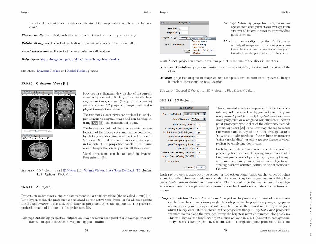
Image . Stacks .

slices for the output stack. In this case, the size of the output stack in determined by Slicecount.

Flip vertically If checked, each slice in the output stack will be flipped vertically.

Rotate 90 degrees If checked, each slice in the output stack will be rotated 90◦.

Avoid interpolation If checked, no interpolation will be done.

Help Opens http://imagej.nih.gov/ij/docs/menus/image.html#reslice.

See also: Dynamic Reslice and Radial Reslice plugins

25.6.10 Orthogonal Views [H]

Provides an orthogonal view display of the currentstack or hyperstack [19]. E.g., if a stack displayssagittal sections, coronal (YZ projection image)and transverse (XZ projection image) will be dis-played through the data-set.

The two extra planar views are displayed in ‘sticky’panels next to original image and can be toggledusing Shift H , the command shortcut.

The intersection point of the three views follows thelocation of the mouse click and can be controlledby clicking and dragging in either the XY, XZ orYZ view. XY and XZ coordinates are displayedin the title of the projection panels. The mousewheel changes the screen plane in all three views.

Voxel dimensions can be adjusted in Image .Properties. . . [P].

See also: 3D Project. . . , and 3D Viewer [13], Volume Viewer, Stack Slicer Display3_TP plugins,Edit .Options .DICOM. . .

25.6.11 Z Project. . .

Projects an image stack along the axis perpendicular to image plane (the so-called z axis) [18].With hyperstacks, the projection s performed on the active time frame, or for all time pointsif All Time Frames is checked. Five different projection types are supported. The preferredprojection method is stored in the preferences file.

Average Intensity projection outputs an image wherein each pixel stores average intensityover all images in stack at corresponding pixel location.


Image . Stacks .

Average Intensity projection outputs an im-age wherein each pixel stores average inten-sity over all images in stack at correspondingpixel location.

Maximum Intensity projection (MIP) createsan output image each of whose pixels con-tains the maximum value over all images inthe stack at the particular pixel location.

Sum Slices projection creates a real image that is the sum of the slices in the stack.

Standard Deviation projection creates a real image containing the standard deviation of theslices.

Median projection outputs an image wherein each pixel stores median intensity over all imagesin stack at corresponding pixel location.

See also: Grouped Z Project. . . , 3D Project. . . , Plot Z-axis Profile. . .

25.6.12 3D Project. . .

This command creates a sequence of projections of arotating volume (stack or hyperstack) onto a planeusing nearest-point (surface), brightest-point, or mean-value projection or a weighted combination of nearestpoint projection with either of the other two methods(partial opacity) [20]. The user may choose to rotatethe volume about any of the three orthogonal axes(x, y, or z), make portions of the volume transparent(using thresholding), or add a greater degree of visualrealism by employing depth cues.

Each frame in the animation sequence is the result ofprojecting from a different viewing angle. To visualizethis, imagine a field of parallel rays passing througha volume containing one or more solid objects andstriking a screen oriented normal to the directions ofthe rays.

Each ray projects a value onto the screen, or projection plane, based on the values of pointsalong its path. Three methods are available for calculating the projections onto this plane:nearest-point, brightest-point, and mean-value. The choice of projection method and the settingsof various visualization parameters determine how both surface and interior structures willappear.

Projection Method Select Nearest Point projection to produce an image of the surfacesvisible from the current viewing angle. At each point in the projection plane, a ray passesnormal to the plane through the volume. The value of the nearest non transparent pointwhich the ray encounters is stored in the projection image. Brightest Point projectionexamines points along the rays, projecting the brightest point encountered along each ray.This will display the brightest objects, such as bone in a CT (computed tomographic)study. Mean Value projection, a modification of brightest–point projection, sums the


The

IJUser

Guid

e—

Bookle

t44

Image . Stacks .

values of all transparent points along each ray and projects their mean value. It producesimages with softer edges and lower contrast, but can be useful when attempting to visualizeobjects contained within a structure of greater brightness (e.g. a skull).

Slice Spacing The interval, in pixels, between the slices that make up the volume. ImageJprojects the volume onto the viewing plane at each Rotation Angle Increment, beginningwith the volume rotated by Initial Angle and ending once the volume has been rotated byTotal Rotation.

Lower /Upper Transparency Bound Determine the transparency of structures in the vol-ume. Projection calculations disregard points having values less than the lower thresholdor greater than the upper threshold. Setting these thresholds permits making backgroundpoints (those not belonging to any structure) invisible. By setting appropriate thresholds,you can strip away layers having reasonably uniform and unique intensity values andhighlight (or make invisible) inner structures. Note that you can also use Image .Adjust .Threshold. . . [T] to set the transparency bounds.

Opacity Can be used to reveal hidden spatial relationships, specially on overlapping objects ofdifferent colors and dimensions. The (surface) Opacity parameter permits the display ofweighted combinations of nearest-point projection with either of the other two methods,often giving the observer the ability to view inner structures through translucent outersurfaces. To enable this feature, set Opacity to a value greater than zero and select eitherMean Value or Brightest Point projection.

Surface / Interior Depth–Cueing Depth cues can contribute to the three-dimensional qual-ity of projection images by giving perspective to projected structures. The depth-cueingparameters determine whether projected points originating near the viewer appear brighter,while points further away are dimmed linearly with distance. The trade-off for this in-creased realism is that data points shown in a depth-cued image no longer possess accuratedensitometric values. Two kinds of depth-cueing are available: Surface Depth-Cueing andInterior Depth-Cueing. Surface Depth-Cueing works only on nearest-point projectionsand the nearest-point component of other projections with opacity turned on. InteriorDepth-Cueing works only on brightest-point projections. For both kinds, depth-cueing isturned off when set to zero (i.e. 100% of intensity in back to 100% of intensity in front) andis on when set at 0 <n 100 (i.e. (100−n)% of intensity in back to 100% intensity in front).Having independent depth-cueing for surface (nearest-point) and interior (brightest-point)allows for more visualization possibilities.

Interpolate Check Interpolate to generate a temporary z-scaled stack that is used to generatethe projections. Z-scaling eliminates the gaps seen in projections of volumes with slicespacing greater than 1.0 pixels. This option is equivalent to using the Scale plugin fromthe TransformJ package to scale the stack in the z-dimension by the slice spacing (inpixels). This checkbox is ignored if the slice spacing is less than or equal to 1.0 pixels.

See also: Orthogonal Views [H], Z Project. . . , Grouped Z Project. . . and 3D Viewer [13], VolumeViewer plugins


Image . Stacks .

25.6.13 Plot Z-axis Profile. . .

Plots the ROI selection mean gray value versusslice number. Requires a point or area selection.

Coordinates of the upper left corner of theselection (or the bounding rectangle for non-rectangular selections) are displayed in the graphtitle.

See also: Profile Plot Options. . . , Plot Profile [k]

25.6.14 Label. . .

Adds a sequence of numbers (e.g., timestamps) and/or a labelto a stack or hyperstack. Numbers and label are drawn inthe current foreground color (cf. Image .Colors .Color Picker. . .[K]).

The initial X,Y location, and Font size of the label are basedon the existing rectangular selection, if any. Slices outside theRange are not affected.

Format Specifies the structure of the label. 0 : Un-padded sequence; 0000 : Pads each number with lead-ing zero(s); 00 : 00 : Converts the label into a min-utes : seconds timestamp; 00 : 00 : 00 Converts the labelinto a hours :minutes : seconds timestamp; Text : Stampsonly the contents of the Text field.

Starting value and Interval Specify the first value and the numeric steps to be applied.Note that with timestamps, metric time values must be used, e.g., an Interval of 3600 willcreate 1 hour increments.

Text The string to be drawn after each number when the Format chosen is either 0 or Text(label without numeric sequence).

Use overlay If checked, labels will be created as non-destructive image overlays. Note thatpreviously added overlays will be removed.

Use text tool font If checked, labels will be created using the type face and style specified inthe Fonts. . . widget.

Help Opens http://imagej.nih.gov/ij/docs/menus/image.html#label.

See also: Make Montage, Stacks .Tools . Insert. . .


The

IJUser

Guid

e—

Bookle

t45

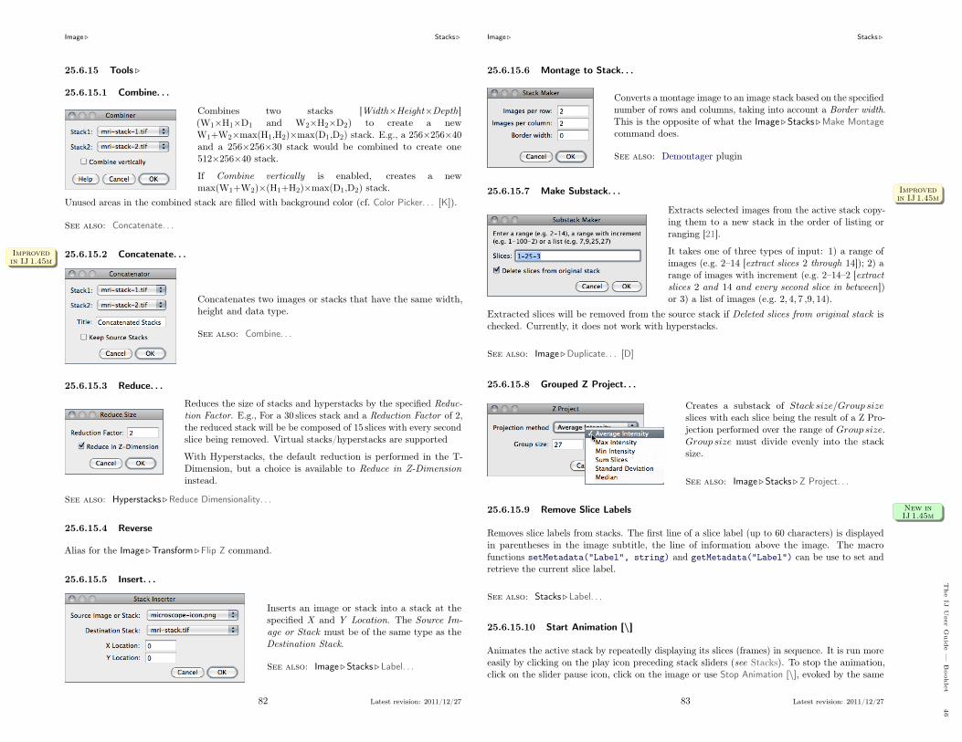
Image . Stacks .

25.6.15 Tools .

25.6.15.1 Combine. . .

Combines two stacks [Width×Height×Depth](W1×H1×D1 and W2×H2×D2) to create a newW1+W2×max(H1,H2)×max(D1,D2) stack. E.g., a 256×256×40and a 256×256×30 stack would be combined to create one512×256×40 stack.

If Combine vertically is enabled, creates a newmax(W1+W2)×(H1+H2)×max(D1,D2) stack.

Unused areas in the combined stack are filled with background color (cf. Color Picker. . . [K]).

See also: Concatenate. . .

25.6.15.2 Concatenate. . .Improvedin IJ 1.45mImprovedin IJ 1.45m

Concatenates two images or stacks that have the same width,height and data type.

See also: Combine. . .

25.6.15.3 Reduce. . .

Reduces the size of stacks and hyperstacks by the specified Reduc-tion Factor. E.g., For a 30 slices stack and a Reduction Factor of 2,the reduced stack will be be composed of 15 slices with every secondslice being removed. Virtual stacks/hyperstacks are supported

With Hyperstacks, the default reduction is performed in the T-Dimension, but a choice is available to Reduce in Z-Dimensioninstead.

See also: Hyperstacks .Reduce Dimensionality. . .

25.6.15.4 Reverse

Alias for the Image .Transform .Flip Z command.

25.6.15.5 Insert. . .

Inserts an image or stack into a stack at thespecified X and Y Location. The Source Im-age or Stack must be of the same type as theDestination Stack.

See also: Image . Stacks . Label. . .


Image . Stacks .

25.6.15.6 Montage to Stack. . .

Converts a montage image to an image stack based on the specifiednumber of rows and columns, taking into account a Border width.This is the opposite of what the Image .Stacks .Make Montagecommand does.

See also: Demontager plugin

25.6.15.7 Make Substack. . . Improvedin IJ 1.45mImprovedin IJ 1.45m

Extracts selected images from the active stack copy-ing them to a new stack in the order of listing orranging [21].

It takes one of three types of input: 1) a range ofimages (e.g. 2–14 [extract slices 2 through 14]); 2) arange of images with increment (e.g. 2–14–2 [extractslices 2 and 14 and every second slice in between])or 3) a list of images (e.g. 2, 4, 7 ,9, 14).

Extracted slices will be removed from the source stack if Deleted slices from original stack ischecked. Currently, it does not work with hyperstacks.

See also: Image .Duplicate. . . [D]

25.6.15.8 Grouped Z Project. . .

Creates a substack of Stack size/Group sizeslices with each slice being the result of a Z Pro-jection performed over the range of Group size.Group size must divide evenly into the stacksize.

See also: Image .Stacks .Z Project. . .

25.6.15.9 Remove Slice Labels New inIJ 1.45mNew inIJ 1.45m

Removes slice labels from stacks. The first line of a slice label (up to 60 characters) is displayedin parentheses in the image subtitle, the line of information above the image. The macrofunctions setMetadata("Label", string) and getMetadata("Label") can be use to set andretrieve the current slice label.

See also: Stacks . Label. . .

25.6.15.10 Start Animation [\]

Animates the active stack by repeatedly displaying its slices (frames) in sequence. It is run moreeasily by clicking on the play icon preceding stack sliders (see Stacks). To stop the animation,click on the slider pause icon, click on the image or use Stop Animation [\], evoked by the same


The

IJUser

Guid

e—

Bookle

t46

Image . Hyperstacks .

shortcut. As such, stacks animation can be toggled using \ . The frame rate is displayed inthe status bar. Open the Animation Options. . . [Alt /] dialog box to specify the animation speed(pressing Alt \ or right-clicking on the on the slider play/pause icon opens the AnimationOptions. . . dialog). Note that more than one stack can be animated at a time.

25.6.15.11 Stop Animation [\]

Terminates animation of the active stack (see Start Animation [\]).

25.6.15.12 Animation Options. . . [Alt /]

Use this dialog to set the animation speed in frames per second,the starting and ending frame, or to enable ‘oscillating’ animations.Selecting Start Animation animates the stack as soon as the dialogis dismissed.

Note that setting the Frame Interval in Image .Properties. . . [P]sets the animation speed as long as the unit used is ‘sec’.

This dialog can also be accessed by right-clicking on the play/pause icon that precedes the sliceslider in Stacks and frame slider in Hyperstacks (see Stacks and Hyperstacks).

See also: File .Save As .Gif. . . , AVI. . .

25.7 Hyperstacks .

This submenu contains commands that work with Hyperstacks, images that have four (4D) orfive (5D) dimensions.

25.7.1 New Hyperstack. . .

Creates a new hyperstack. Hyperstacks haveWidth, Height,Channels (c dimension), Slices (z dimension) and timeFrames (t dimension).

Image Type (see Image .Type . ) and Display Mode (seeChannels Tool. . . [Z]) can be specified.

Checking Label Images will draw the channel number, slicenumber and frame number on each image in the hyperstack.

File .New .Hyperstack. . . is an alias of this command.


Image . Crop [X]

25.7.2 Stack to Hyperstack. . .

Converts a stack into a hyperstack. RGB stacks areconverted into 3 channel hyperstacks.

Order is the order of the channels (c), slices (z ) andframes (t) within the stack. ImageJ hyperstacks arealways in czt order. Stacks not in czt order will beshuffled to be in czt order. The channel Display Modecan be Composite, Color or Grayscale (cf. ChannelsTool. . . [Z]).

See also: Hyperstack to Stack

25.7.3 Hyperstack to Stack

Converts a hyperstack into a stack (in czt order).

See also: Stack to Hyperstack. . .

25.7.4 Reduce Dimensionality. . .

This command [22] reduces the dimensionality of an hyperstack bycreating a new hyperstack with, for example, all the channels and timepoints at a given z position or all the z slices for the current channeland time point.

Uncheck Channels (n) to delete all but the current channel, Slices (n)to delete all but the current z slice and Frames (n) to delete all but thecurrent time point. Check Keep Source and the original stack will notbe deleted.

The expected dimensions and size of the reduced stack are displayed inthe dialog.

See also: Hyperstack to Stack

25.7.5 Channels Tool. . . [Z]

Opens the Channels. . . widget, or brings it to the front if it is already open. Shift Z is thekeyboard shortcut for this command. This tool allows to select the Display mode of compositeimages. In addition, several commands hosted in the Image .Color . submenu can easily beaccessed through the More� drop-down menu. The same drop-down menu also provides aconvenient list of primary colors (additive: red, green and blue, subtractive: cyan, magenta,yellow) that can be used to pseudocolor composite channels. Composite images are discussedwith more detail in Color Composites.

25.8 Crop [X]

Crops the image or stack based on the current rectangular selection.


The

IJUser

Guid

e—

Bookle

t47

Image . Duplicate. . . [D]

Channel manipulations in composite images using the Image .Color .Channels Tool. . . [Z]tool.

25.9 Duplicate. . . [D]

Creates a new window containing a copy of the active image orrectangular selection. For stacks and hyperstacks it is possible tospecify the range of Channels (c), Slices (z) and Frames (t) to beduplicated.

With single images, hold Alt to skip the dialog box.

25.10 Rename. . .

Renames the active image.

25.11 Scale. . . [E]Improvedin IJ 1.45mImprovedin IJ 1.45m

Resizes the image or current area selection by scale factorsentered into a dialog box. As with Image . Size. . . , two resam-pling methods are possible: Bilinear and Bicubic interpolation.

For the best looking results, particularly with graphics andtext, use integer scale factors (2, 3, 5, etc.) and check Averagewhen downsizing with scale factors less than 1.0 [16]. Also,when downsizing, smoothing the source image prior to scalingmay produce better looking results.

Scaled image/selection are copied to a new image named Titleif Create new window is checked. If scaling a selection thatwill not be copied to a new image check Fill with BackgroundColor to fill with the background color instead of zero.

Entire stacks (or hyperstacks in the Z Dimension) will bescaled if Process entire stack is checked.


Image . Transform .

25.12 Transform .

This submenu contains commands that perform geometrical image transformation on the activeimage or stack.

25.12.1 Flip Horizontally

Replaces the image or selection with a x-mirror image of the original.

25.12.2 Flip Vertically

Turns the image or selection upside down (y-mirror).

25.12.3 Flip Z

Reverses the order of the slices in a stack (z-mirror).

25.12.4 Rotate 90 Degrees Right

Rotates the entire image or stack clockwise 90◦.

25.12.5 Rotate 90 Degrees Left

Rotates the entire image or stack counter-clockwise 90◦.

25.12.6 Rotate. . .

Use this dialog to rotate the active im-age or selection clockwise the specifiednumber of degrees.

Set Grid Lines to a value greater thanzero to superimpose a grid on the im-age in Preview mode. Two resam-pling methods are possible: Bilinearand Bicubic interpolation (cf. Image .Size. . . ).

With 8–bit and RGB images, check Fill with Background Color to fill with the backgroundcolor instead of zero (cf. Color Picker. . . [K]). Check Enlarge to Fit Result and the image will beenlarged as needed to avoid clipping.

25.12.7 Translate. . .

Translates (moves) the image in the x and y directions by aspecified number of pixels. With stacks, you can translate eitherthe current image or all the images in the stack. Two resamplingmethods are possible: Bilinear and Bicubic interpolation (cf.Image . Size. . . ).

Check Preview to see how the translation will affect the image.The background at the edges of the image will be set to 0.


The

IJUser

Guid

e—

Bookle

t48

Image . Zoom .

See also: Align_Slice and Align_RGB_planes plugins

25.13 Zoom .

This submenu contains commands that control how the current image is displayed. The +

and − or ↑ and ↓ keys are the preferred way to use the In and Out commands. When aselection exists, zooming with the arrow keys requires holding down either Shift or Ctrl .

25.13.1 In [+]

Zooms in to next higher magnification level and, if possible, enlarges the window. There are21 possible levels (shown in the title bar): 3.1, 4.2, 6.3, 8.3, 12.5, 16.7, 25, 33.3, 50, 75, 100, 150,200, 300, 400, 600, 800, 1200, 1600, 2400 and 3200%.

XVIII Scrolling Zoomed ImagesHold down the space bar and drag to scroll a zoomed image.

25.13.2 Out [-]

Zooms out to next lower magnification level and, if needed, shrinks the window.

25.13.3 Original Scale [4]

Displays the image at the magnification used when the image was first opened. As a shortcut,double click on the magnifying glass tool.

25.13.4 View 100% [5]

Displays the image using 100% magnification (1 image pixel = 1 screen pixel). Enable OpenImages at 100% in the Edit .Options .Appearance. . . dialog to have images automaticallyopened at 100% magnification.

25.13.5 To Selection

Zooms in based on the current selection. Note that in the absence of a selection, this commandzooms the image to a ‘Fit to Screen’ level.

25.13.6 Set. . .Improvedin IJ 1.45mImprovedin IJ 1.45m

Zooms the active image to an exact value (e.g. 37.4%) overcoming thepredefined zoom steps described in Image .Zoom . 25.13.1. The zoomedcanvas will be centered at X,Y center (pixel coordinates) [23].


Image . Overlay .

25.14 Overlay .

This submenu contains commands for creating and working with non-destructive image overlays.An overlay consists of one or more selections: arrows, lines, points, shapes and text (see ImageJToolbar). Overlays can also be composed of image selections (imageROIs) that behave partiallyas regular selections (see Add Image. . . ).

Press B (Add Selection. . . [b]) to add the current selection to the overlay. Press Shift F(Flatten [F]) to create an RGB image with the overlay embedded in it. The overlay is preservedwhen an image is saved in TIFF format (cf. II Image Types: Lossy Compression and Metadata).

Non-destructive image overlays. Outputs from Grid_Overlay, MakeOverlay and ROI Color Coder,macros that exemplify the usage of most Image .Overlay . submenu commands.

25.14.1 Add Selection. . . [b]

Adds the current selection to the overlay, displaying the dialog boxdepicted on the left. Stroke Color, Stroke Width and Fill Colorto be set. Except for text selections, and as explained in Edit .Selection .Properties. . . [y], the stroke (line) color and width areignored if a fill color is specified.

Colors are specified using the name of one of the eight default colors(black, blue, cyan, green, magenta, red, white and yellow) or usinghex notation (see XIX Hexadecimal Color Values).

Holding Alt will immediately add the selection to the overlayskipping this dialog. Previously added overlays are removed if NewOverlay is checked.

See also: Selection .Properties. . . [y], ROI Manager. . . , XIX Hexadecimal Color Values, ROIColor Coder and RGBtoHEX macros

25.14.2 Add Image. . . Improvedin IJ 1.45mImprovedin IJ 1.45m

Adds an image to the overlay (Overlays two open images). A blending alpha value can bespecified in the Opacity (0–100%) field. The initial X,Y location is based on the existingrectangular selection, if any.


The

IJUser

Guid

e—

Bookle

t49

Image . Overlay .

Select Create image selection to create an overlay image thatcan be moved around the canvas. Opacity of image selec-tions (ImageROIs) can be adjusted at any time using Edit .Selection .Properties. . . [y]. Use Shift E (Edit .Selection .Restore Selection [E]) to recover the blending image after click-ing outside its limits. Use Shift F (Flatten [F]) to finallyembed the imageROI.

Note that image selections behave only partially as regularselections (e.g., can be added to the ROI Manager list, canbe moved beyond image boundaries but cannot be resized orrotated). In addition, image selections are not saved in theTIFF header.

See also: Paste Control. . . (Blend transfer mode), ROI Manager. . .

25.14.3 Hide Overlay

Causes ImageJ to stop displaying the overlay displayed by Show Overlay.

25.14.4 Show Overlay

Displays an overlay that was hidden by Hide Overlay.

25.14.5 From ROI Manager

Creates an overlay from the selections on the ROI Manager list (see ROI Manager. . . ). Notethat previously added overlays will be removed.

25.14.6 To ROI Manager

Copies the selections and images in the current overlay to the ROI Manager, where they can beedited (moved, resized or re-colored) (see ROI Manager. . . ). Note that previous items in theROI Manager list will be deleted.

25.14.7 Remove Overlay

Permanently clears the overlay so that it cannot be restored using Show Overlay.

25.14.8 Flatten [F]

Creates a new RGB image that has the overlay rendered as pixel data. The RGB image isthe same size as the active image, unlike Plugins .Utilities .Capture Image, which creates aWYSIWYG (What You See Is What You Get) image that is the same size as its window.


Image . Lookup Tables .

25.15 Lookup Tables .

This submenu contains a selection of color lookup tables that can be applied to grayscale imagesto produce false-color images. If no image is open, a 256×32 ramp image is created to display thecolor table. More than 100 additional lookup tables are available at imagej.nih.gov/ij/download/luts/ or, as a ZIP archive, at http://imagej.nih.gov/ij/download/luts/luts.zip.

See also: Toolset Switcher

25.15.1 Invert LUT

Inverts the current lookup table. For 8–bit images, the value (v) of each entry in the table isreplaced by 255− v. With inverted LUTs, pixels with a value of zero are white and pixels witha value 255 are black. Unlike the Edit . Invert [I] command, pixels values are not altered, only theway the image is displayed on the screen.

25.15.2 Apply LUT

Applies the current lookup table function to each pixel in the image or selection and restoresthe default identity function. This modifies the gray values so that when the image is viewedusing the default grayscale lookup table it will look the same as it did before. This command isequivalent to clicking on Apply in Image .Adjust .Brightness/Contrast. . . [C]. For thresholdedimages, it is equivalent to clicking on Apply in Image .Adjust .Threshold. . . [T].


The

IJUser

Guid

e—

Bookle

t50

Image . Lookup Tables .

XIX Hexadecimal Color Values

Hexadecimal (hex) notation is frequently used in computing to summarize binary code in ahuman-friendly manner. Here are some decimal/hexadecimal equivalents:

Dec 0 1 2 3 4 5 6 7 8 9 10 11 12 13 14 15 16 17 18 19 20 . . . 30 40 50 60 70 80 90 100 110 . . . 255Hex 0 1 2 3 4 5 6 7 8 9 A B C D E F 10 11 12 13 14 . . . 1E 28 32 3C 46 50 5A 64 6E . . . FF

Decimal RGB color values that typically range from 0 to 255 are succinctly represented bytwo hexadecimal digits ranging from 00 through FF. A hex color value is a 6–digit, three–bytehexadecimal number (hex triplet) in the form #RRGGBB, in which RR specifies the red, GGthe green and BB the blue value.

Opacity of hex triplets can be modified by an optional transparency (alpha) channel, givingrise to a 8–digit, four–byte hex number in the form #AARRGGBB with AA specifying thealpha blending value. In ImageJ, the alpha channel codes for opacity and ranges from 00 (fullytransparent) to FF (solid color). Alpha values can be omitted for fully opaque colors. The tablebelow provides some hexadecimal color values in 10% transparency increments.

Color RGB tripletOpacity value (optional)

Hex triplet0% 10% 20% 30% 40% 50% 60% 70% 80% 90% 100%

Blue 0, 0, 255 #FF #E5 #CC #B2 #99 #7F #66 #4C #33 #19 #00 00 00FFCyan 0, 255, 255 #FF #E5 #CC #B2 #99 #7F #66 #4C #33 #19 #00 00FFFFGreen 0, 255, 0 #FF #E5 #CC #B2 #99 #7F #66 #4C #33 #19 #00 00FF00Magenta 255, 0, 255 #FF #E5 #CC #B2 #99 #7F #66 #4C #33 #19 #00 FF00FFRed 255, 0, 0 #FF #E5 #CC #B2 #99 #7F #66 #4C #33 #19 #00 FF00 00Orange 255, 150, 0 #FF #E5 #CC #B2 #99 #7F #66 #4C #33 #19 #00 FF96 00Yellow 255, 255, 0 #FF #E5 #CC #B2 #99 #7F #66 #4C #33 #19 #00 FFFF00White 255, 255, 255 #FF #E5 #CC #B2 #99 #7F #66 #4C #33 #19 #00 FFFFFFGray 127, 127, 127 #FF #E5 #CC #B2 #99 #7F #66 #4C #33 #19 #00 7F 7F 7FBlack 0, 0, 0 #FF #E5 #CC #B2 #99 #7F #66 #4C #33 #19 #00 00 00 00

Alpha blending values can be added to the beginning of hex triplets to modulate the color transparency:e.g., #7FFF00 00 defines red at 50% opacity. In ImageJ the hash (#) prefix is optional when specifyingoverlay colors (see Image .Overlay . ).

The built-in macro function toHex() returns hexadecimal representations of decimal numbersand can be used to convert RGB color values into hex color notation (see RGBtoHEX macro).Several other macros (e.g., MakeOverlay) exemplify how to annotate images using hex colors.


Process .

26 Process .

This menu lists all commands related to image processing, including point operations, filters,and arithmetic operations between multiple images [51]. The File .Open Samples . .Blobs (25K)[B] image will be used in most of the illustrations of this section.

Process . submenu: Smooth [S], Sharpen, Find Edges and Enhance Contrast

26.1 Smooth [S]

Blurs the active image or selection. This filter replaces each pixel with the average of its 3×3neighborhood.

26.2 Sharpen

Increases contrast and accentuates detail in the image or selection, but may also accentuatenoise. This filter uses the following weighting factors to replace each pixel with a weightedaverage of the 3×3 neighborhood:

−1 −1 −1−1 12 −1−1 −1 −1

26.3 Find Edges

Uses a Sobel edge detector to highlight sharp changes in intensity in the active image orselection. Two 3×3 convolution kernels (shown below) are used to generate vertical andhorizontal derivatives. The final image is produced by combining the two derivatives using thesquare root of the sum of the squares.

1 2 1 1 0 −10 0 0 2 0 −2−1 −2 −1 1 0 −1

26.4 Find Maxima. . . Improvedin IJ 1.45mImprovedin IJ 1.45m

Determines the local maxima in an image and creates a binary (mask-like) image of the same sizewith the maxima, or one segmented particle per maximum, marked [24]. Analysis is performedon the existing rectangular selection or on the entire image if no selection is present.

For RGB images, maxima of luminance are selected, with the luminance defined as weighted orunweighted average of the colors depending on how Weighted RGB to Grayscale Conversion isset in Edit .Options .Conversions. . . .


The

IJUser

Guid

e—

Bookle

t51

Process . Find Maxima. . .

Noise Tolerance Maxima are ig-nored if they do not stand outfrom the surroundings by morethan this value (calibrated unitsfor calibrated images). In otherwords, a threshold is set at themaximum value minus noisetolerance and the contiguousarea around the maximum abovethe threshold is analyzed. Foraccepting a maximum, this areamust not contain any pointwith a value higher at than themaximum. Only one maximumwithin this area is accepted.

Output Type Can be (see Process .Find Maxima. . . outputs):

Single Points Results in one single point per maximum.Maxima Within Tolerance All points within the Noise Tolerance for each maximum.Segmented Particles Assumes that each maximum belongs to a particle and segments

the image by a watershed algorithm applied to the values of the image (in contrastto Process .Binary .Watershed, which uses the Euclidian distance map – EDM). SeeProcess .Binary .Voronoi for EDM-based segmentation of binary images.

Point Selection Displays a multi-point selection with a point at each maximum.List Displays the XY coordinates of each maximum in the Results window.Count Displays the number of maxima in the Results window.

Exclude Edge Maxima Excludes maxima if the area within the noise tolerance surroundinga maximum touches the edge of the image (edge of the selection does not matter).

Above Lower Threshold (Thresholded images only) Finds maxima above the lower thresholdonly. The upper threshold of the image is ignored. If Segmented Particles is selected asOutput Type, the area below the lower threshold is considered a background. This optioncannot be used when finding minima (image with light background and inverted LUT).

Light Background To be checked if the image background is brighter than the objects to befound, as it is in the Cell Colony image in the illustration below.

Help Opens http://imagej.nih.gov/ij/docs/menus/process.html#find-maxima.

Output is a binary image, with foreground 255 and background 0, using an inverted or normalLUT depending on the Black Background option in Process .Binary .Options. . . (see XXIInterpreting Binary Images).

The number of particles (as obtained by Analyze .Analyze Particles. . . ) in the output image doesnot depend on the selected Output Type. Note that Segmented Particles will usually result inparticles touching the edge if Exclude Edge Maxima is selected. Exclude Edge Maxima appliesto the maximum, not to the particle.

Find Maxima. . . does not work on stacks, but the FindStackMaxima macro runs it on all theimages in a stack and creates a second stack containing the output images. The FindMaxi-maRoiManager macro demonstrates how to add particles found by Find Maxima. . . to the ROIManager. . .


Process . Enhance Contrast

Process . Find Maxima. . . (ImageJ 1.43s). Six outputs are possible: Single Points, Maxima WithinTolerance, Segmented Particles, Point Selection, List and Count.

Points at maxima (Multi-point selection) Segmented Particles (ROIs obtained with Analyze .Analyze Particles. . . )

26.5 Enhance Contrast

Enhances image contrast by using either histogram stretching orhistogram equalization. Both methods are described in detail in theHypermedia Image Processing Reference – Contrast Stretching andHistogram Equalization.

This command does not alter pixel values as long as Normalize,Equalize Histogram or Normalize All n Slices (in the case of stacks)are not checked.

Saturated Pixels Determines the number of pixels in the image that are allowed to becomesaturated. Increasing this value will increase contrast. This value should be greater thanzero to prevent a few outlying pixel from causing the histogram stretch to not work asintended.

Normalize If checked, ImageJ will recalculate the pixel values of the image so the range isequal to the maximum range for the data type, or 0–1.0 for float images. The contraststretch performed on the image is similar to the ‘Auto’ option in the Brightness/Contrast. . .[C] window, except that with stacks, each slice in the stack is adjusted independently,according to the optimal for that slice alone (if Use Stack Histogram is unchecked). Themaximum range is 0–255 for 8–bit images and 0–65535 for 16–bit images.With stacks another checkbox, Normalize All n Slices, is displayed. If checked, normaliza-tion will be applied to all slices in the stack. Note that normalization of RGB images isnot supported, and thus this option will not be available on RGB images.

Equalize Histogram If checked, ImageJ will enhance the image using histogram equalization[25]. Create a selection and the equalization will be based on the histogram of the selection.Uses a modified algorithm that takes the square root of the histogram values. Hold Alt touse the standard histogram equalization algorithm. The Saturated Pixels and Normalizeparameters are ignored when Equalize Histogram is checked.


The

IJUser

Guid

e—

Bookle

t52

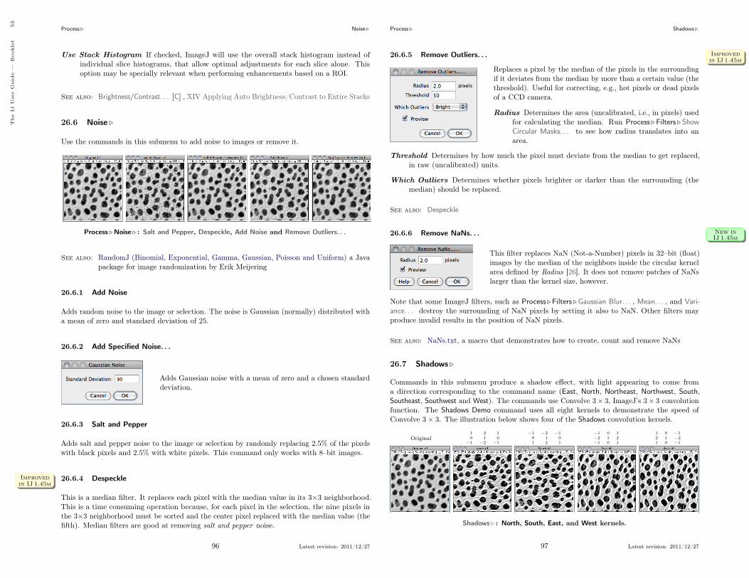
Process . Noise .

Use Stack Histogram If checked, ImageJ will use the overall stack histogram instead ofindividual slice histograms, that allow optimal adjustments for each slice alone. Thisoption may be specially relevant when performing enhancements based on a ROI.

See also: Brightness/Contrast. . . [C] , XIV Applying Auto Brightness/Contrast to Entire Stacks

26.6 Noise .

Use the commands in this submenu to add noise to images or remove it.

Process .Noise . : Salt and Pepper, Despeckle, Add Noise and Remove Outliers. . .

See also: RandomJ (Binomial, Exponential, Gamma, Gaussian, Poisson and Uniform) a Javapackage for image randomization by Erik Meijering

26.6.1 Add Noise

Adds random noise to the image or selection. The noise is Gaussian (normally) distributed witha mean of zero and standard deviation of 25.

26.6.2 Add Specified Noise. . .

Adds Gaussian noise with a mean of zero and a chosen standarddeviation.

26.6.3 Salt and Pepper

Adds salt and pepper noise to the image or selection by randomly replacing 2.5% of the pixelswith black pixels and 2.5% with white pixels. This command only works with 8–bit images.

26.6.4 DespeckleImprovedin IJ 1.45mImprovedin IJ 1.45m

This is a median filter. It replaces each pixel with the median value in its 3×3 neighborhood.This is a time consuming operation because, for each pixel in the selection, the nine pixels inthe 3×3 neighborhood must be sorted and the center pixel replaced with the median value (thefifth). Median filters are good at removing salt and pepper noise.


Process . Shadows .

26.6.5 Remove Outliers. . . Improvedin IJ 1.45mImprovedin IJ 1.45m

Replaces a pixel by the median of the pixels in the surroundingif it deviates from the median by more than a certain value (thethreshold). Useful for correcting, e.g., hot pixels or dead pixelsof a CCD camera.

Radius Determines the area (uncalibrated, i.e., in pixels) usedfor calculating the median. Run Process .Filters .ShowCircular Masks. . . to see how radius translates into anarea.

Threshold Determines by how much the pixel must deviate from the median to get replaced,in raw (uncalibrated) units.

Which Outliers Determines whether pixels brighter or darker than the surrounding (themedian) should be replaced.

See also: Despeckle

26.6.6 Remove NaNs. . . New inIJ 1.45mNew inIJ 1.45m

This filter replaces NaN (Not-a-Number) pixels in 32–bit (float)images by the median of the neighbors inside the circular kernelarea defined by Radius [26]. It does not remove patches of NaNslarger than the kernel size, however.

Note that some ImageJ filters, such as Process .Filters .Gaussian Blur. . . , Mean. . . , and Vari-ance. . . destroy the surrounding of NaN pixels by setting it also to NaN. Other filters mayproduce invalid results in the position of NaN pixels.

See also: NaNs.txt, a macro that demonstrates how to create, count and remove NaNs

26.7 Shadows .

Commands in this submenu produce a shadow effect, with light appearing to come froma direction corresponding to the command name (East, North, Northeast, Northwest, South,Southeast, Southwest and West). The commands use Convolve 3× 3, ImageJ’s 3× 3 convolutionfunction. The Shadows Demo command uses all eight kernels to demonstrate the speed ofConvolve 3× 3. The illustration below shows four of the Shadows convolution kernels.

Original1 2 10 1 0

−1 −2 −1

−1 −2 −10 1 01 2 1

−1 0 1−2 1 2−1 0 1

1 0 −12 1 −21 0 −1

Shadows . : North, South, East, and West kernels.


The

IJUser

Guid

e—

Bookle

t53

Process . Binary .

26.8 Binary .

This submenu contains commands that create or process binary (black and white) images. Theyassume that objects are black and background is white unless Black Background is checked inthe Process .Binary .Options. . . dialog box (see XXI Interpreting Binary Images).

Summary of morphological operators (Process .Binary . submenu).Original Make Binary Erode Dilate Open Close– Outline Skeletonize

Adjust .Threshold. . . [T] Minimum. . .(grayscale)

Maximum. . .(grayscale)

Erode thenDilate

Dilate thenErode

1 pixel wideoutline

1 pixel wideskeleton

26.8.1 Make Binary

Converts an image to black and white. If a threshold hasbeen set using the Image .Adjust .Threshold. . . [T] tool,the depicted dialog is displayed. The value of the Blackforeground, white background checkbox reflects and setsthe global Black Background value of Process .Binary .Options. . .

If a threshold has not been set, Make Binary will analyze the histogram of the current selection,or of the entire image if there is no selection is present and set an automatic threshold level tocreate the binary image (‘Auto-thresholding ’ is displayed in the Status bar, cf. Threshold. . . [T]).

With stacks the Convert to Mask dialog box is displayed. Note that for non-thresholded imagesand stacks Make Binary and Convert to Mask behave similarly.

See also: Edit .Selection .Convert to Mask, XX Creating Binary Masks, XXI InterpretingBinary Images

26.8.2 Convert to Mask

Converts an image to black and white.

The mask will have an inverting LUT (white is 0 and blackis 255) unless Black Background is checked in the Process .Binary .Options. . . dialog box. If a threshold has not beenset, automatic threshold levels will be calculated (cf. MakeBinary). Note that for non-thresholded images and stacksMake Binary and Convert to Mask behave similarly.

With stacks, the depicted dialog is displayed.

Calculate Threshold for Each Image If checked, threshold levels will be calculated foreach individual slice, otherwise the calculated threshold of the currently displayed slicewill be used for all slices

Black Background Defines whether the background is black and the foreground is white.Note that the value of this checkbox reflects and sets the global Black Background valueof Process .Binary .Options. . .

See also: Make Binary, Edit . Selection .Convert to Mask, XX Creating Binary Masks,


Process . Binary .

XX Creating Binary MasksFour ImageJ commands can be used to create binary masks:

1. Edit . Selection .Create Mask

2. Process .Binary .Make Binary

3. Process .Binary .Convert to Mask

4. Image .Adjust .Threshold. . . [T] (Apply)

By default these commands will produce binary images with inverted LUTs, so that black is 255and white is 0 (see Invert LUT). This behavior can be reversed by checking Black Backgroundin Process .Binary .Options. . . before running the above commands (i.e., an inverting LUTwill not be used: black will be 0 and white 255). This choice can be confirmed when runningMake Binary and Convert to Mask on thresholded images. It can also be imposed at startup (seeSettings and Preferences).

See also: XXI Interpreting Binary Images

26.8.3 Erode

Removes pixels from the edges of objects in a binary image. Use Filters .Minimum. . . to performgrayscale erosion on non-thresholded images.

See also: Binary .Options. . . , XXI Interpreting Binary Images

26.8.4 Dilate

Adds pixels to the edges of objects in a binary image. Use Filters .Maximum. . . to performgrayscale dilation on non-thresholded images.


26.8.5 Open

Performs an erosion operation, followed by dilation. This smoothes objects and removes isolatedpixels.


26.8.6 Close–

Performs a dilation operation, followed by erosion. This smoothes objects and fills in smallholes. The command has a tailing hyphen to differentiate it from File .Close [w] .



The

IJUser

Guid

e—

Bookle

t54

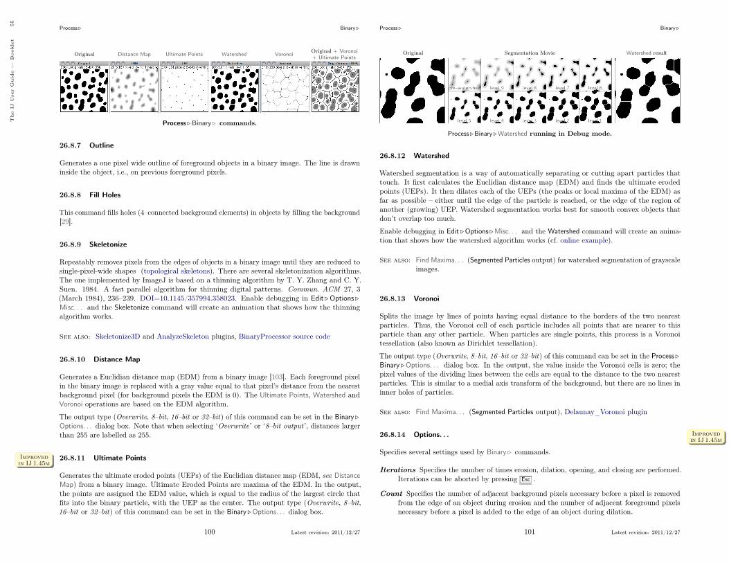
Process . Binary .

Original Distance Map Ultimate Points Watershed Voronoi Original + Voronoi+ Ultimate Points

Process .Binary . commands.

26.8.7 Outline

Generates a one pixel wide outline of foreground objects in a binary image. The line is drawninside the object, i.e., on previous foreground pixels.

26.8.8 Fill Holes

This command fills holes (4–connected background elements) in objects by filling the background[29].

26.8.9 Skeletonize

Repeatably removes pixels from the edges of objects in a binary image until they are reduced tosingle-pixel-wide shapes (topological skeletons). There are several skeletonization algorithms.The one implemented by ImageJ is based on a thinning algorithm by T. Y. Zhang and C. Y.Suen. 1984. A fast parallel algorithm for thinning digital patterns. Commun. ACM 27, 3(March 1984), 236–239. DOI=10.1145/357994.358023. Enable debugging in Edit .Options .Misc. . . and the Skeletonize command will create an animation that shows how the thinningalgorithm works.

See also: Skeletonize3D and AnalyzeSkeleton plugins, BinaryProcessor source code

26.8.10 Distance Map

Generates a Euclidian distance map (EDM) from a binary image [103]. Each foreground pixelin the binary image is replaced with a gray value equal to that pixel’s distance from the nearestbackground pixel (for background pixels the EDM is 0). The Ultimate Points, Watershed andVoronoi operations are based on the EDM algorithm.

The output type (Overwrite, 8–bit, 16–bit or 32–bit) of this command can be set in the Binary .Options. . . dialog box. Note that when selecting ‘Overwrite’ or ‘8–bit output ’, distances largerthan 255 are labelled as 255.

26.8.11 Ultimate PointsImprovedin IJ 1.45mImprovedin IJ 1.45m

Generates the ultimate eroded points (UEPs) of the Euclidian distance map (EDM, see DistanceMap) from a binary image. Ultimate Eroded Points are maxima of the EDM. In the output,the points are assigned the EDM value, which is equal to the radius of the largest circle thatfits into the binary particle, with the UEP as the center. The output type (Overwrite, 8–bit,16–bit or 32–bit) of this command can be set in the Binary .Options. . . dialog box.


Process . Binary .

Original Segmentation Movie Watershed result

Process .Binary .Watershed running in Debug mode.

26.8.12 Watershed

Watershed segmentation is a way of automatically separating or cutting apart particles thattouch. It first calculates the Euclidian distance map (EDM) and finds the ultimate erodedpoints (UEPs). It then dilates each of the UEPs (the peaks or local maxima of the EDM) asfar as possible – either until the edge of the particle is reached, or the edge of the region ofanother (growing) UEP. Watershed segmentation works best for smooth convex objects thatdon’t overlap too much.

Enable debugging in Edit .Options .Misc. . . and the Watershed command will create an anima-tion that shows how the watershed algorithm works (cf. online example).

See also: Find Maxima. . . (Segmented Particles output) for watershed segmentation of grayscaleimages.

26.8.13 Voronoi

Splits the image by lines of points having equal distance to the borders of the two nearestparticles. Thus, the Voronoi cell of each particle includes all points that are nearer to thisparticle than any other particle. When particles are single points, this process is a Voronoitessellation (also known as Dirichlet tessellation).

The output type (Overwrite, 8–bit, 16–bit or 32–bit) of this command can be set in the Process .Binary .Options. . . dialog box. In the output, the value inside the Voronoi cells is zero; thepixel values of the dividing lines between the cells are equal to the distance to the two nearestparticles. This is similar to a medial axis transform of the background, but there are no lines ininner holes of particles.

See also: Find Maxima. . . (Segmented Particles output), Delaunay_Voronoi plugin

26.8.14 Options. . . Improvedin IJ 1.45mImprovedin IJ 1.45m

Specifies several settings used by Binary . commands.

Iterations Specifies the number of times erosion, dilation, opening, and closing are performed.Iterations can be aborted by pressing Esc .

Count Specifies the number of adjacent background pixels necessary before a pixel is removedfrom the edge of an object during erosion and the number of adjacent foreground pixelsnecessary before a pixel is added to the edge of an object during dilation.


The

IJUser

Guid

e—

Bookle

t55

Process . Math .

Black background If checked, binary images willbe created without using an inverted LUT(cf. XX Creating Binary Masks) and com-mands in the Process .Binary . submenu willassume that images contain white objects ona black background (see XXI Interpreting Bi-nary Images). Macros can set this optionusing setOption("BlackBackground", true);(see XXI Interpreting Binary Images and Settingsand Preferences).

Pad edges when eroding If checked, Binary .Erodedoes not erode from the edges of the image. Thissetting also affects Binary .Close–, which erodesfrom the edges unless this checkbox is selected.

Black background If checked, binary images will be created without using an inverted LUT (cf.XX Creating Binary Masks) and commands in the Process .Binary . submenu will assumethat images contain white objects on a black background (see XXI Interpreting BinaryImages). Macros can set this option using setOption("BlackBackground", true); (seeXXI Interpreting Binary Images and Settings and Preferences).

Pad edges when eroding If checked, Binary .Erode does not erode from the edges of theimage. This setting also affects Binary .Close–, which erodes from the edges unless thischeckbox is selected.

EDM output Determines the output type for the Binary .Distance Map, Ultimate Points andVoronoi commands. Set it to ‘Overwrite’ for 8–bit output that overwrites the input image;‘8–bit ’, ‘16–bit ’ or ‘32–bit ’ for separate output images. 32–bit output has floating point(subpixel) distance resolution.

Do This drop-down menu allows to test the chosen settings by previewing each binary operationImprovedin IJ 1.45mImprovedin IJ 1.45m (Erode, Dilate, Open, Close–, Outline, Fill Holes, Skeletonize) on the active image. This

option is only available when the active image is binary.

Help Opens http://imagej.nih.gov/ij/docs/menus/process.html#options.

26.9 Math .

The commands in this submenu add (subtract, multiply, etc.) a constant to each pixel in theactive image or selection. A ‘Preview ’ option is available for most operations.

With stacks, the dialog depicted on the left is displayed.Choose ‘Yes’ to process entire stack or ‘No’ to process onlythe active slice. The dialog is not displayed if Hide "ProcessStack?" dialog is checked in Edit .Options .Misc. . .

See also: Memory & Threads. . .

26.9.1 Add. . .

Adds a constant to the image or selection. With 8–bit images, results greater than 255 are setto 255. With 16–bit signed images, results greater than 65,535 are set to 65,535.


Process . Math .

XXI Interpreting Binary ImagesBinary images are thresholded to only two values, typically 0 and 1, but often – as with ImageJ– 0 and 255, that represent black and white on an 8–bit scale (see Image Types and Formats).

The interpretation of binary images is not universal. While some software packages will alwaysperform binary operations on 255 values (or 1, or any non-zero value), ImageJ takes into accountthe foreground and background colors of the binary image.

0: Black (Background), 255:White

0:White (Background), 255: Black

In ImageJ, the Black background option in Process .Binary .Options. . . defines not only how new binary images will becreated (see XX Creating Binary Masks) but also how previouslycreated images are interpreted. This means object(s) will beinferred on a image-per-image basis. As such, inverting theLUT (see Invert LUT) of a binary image without updating theBlack background option may lead to unexpected results, such asthe aberrant thinning operation (Process .Binary .Skeletonize)depicted here. This issue can be avoided by imposing adequatepreferences at startup, as described in Settings and Preferences.

You can use the Process .Binary .Options. . . dialog to assess theimpact of the Black background option: Create a binary image,choose an operation from the Do drop-down menu, activate thepreview feature and toggle the Black background checkbox.

See also: Settings and Preferences, XX Creating BinaryMasks

26.9.2 Subtract. . .

Subtracts a constant from the image or selection. With 8–bit and 16–bit images, results lessthan 0 are set to 0.

26.9.3 Multiply. . .

Multiplies the image or selection by the specified real constant. With 8–bit images, resultsgreater than 255 are set to 255. With 16–bit signed images, results greater than 65, 535 are setto 65, 535.

26.9.4 Divide. . .

Divides the image or selection by the specified real constant. Except for 32–bit (float) images,attempts to divide by zero are ignored. With 32–bit images, dividing by zero results in Infinity,-Infinity or NaN (0/0) pixels when the source pixels are positive, negative or zero. Thedivide-by-zero value can be redefined using Edit .Options .Misc. . . .

26.9.5 AND. . .

Does a bitwise AND of the image and the specified binary constant.


The

IJUser

Guid

e—

Bookle

t56

Process . Math .

26.9.6 OR. . .

Does a bitwise OR of the image and the specified binary constant.

26.9.7 XOR. . .

Does a bitwise XOR of the image and the specified binary constant.

26.9.8 Min. . .

Pixels in the image with a value less than the specified constant are replaced by the constant.

26.9.9 Max. . .

Pixels in the image with a value greater than the specified constant are replaced by the constant.

26.9.10 Gamma. . .

Applies the function f(p) = (p/255)γ × 255 to each pixel (p) inthe image or selection, where 0.1 ≤ γ ≥ 5.0. For RGB images,this function is applied to all three color channels. For 16–bitimages, the image min and max are used for scaling instead of255.

See also: GammaCorrectionTool macro

26.9.11 Set. . .

Fills the image or selection with the specified value.

26.9.12 Log

For 8–bit images, applies the function f(p) = ln(p)× 255/ ln(255) to each pixel (p) in the imageor selection. For RGB images, this function is applied to all three color channels. For 16–bitimages, the image min and max are used for scaling instead of 255. For float images, no scaling isdone. To calculate log10 of the image, multiply the result of this operation by 0.4343 (1/ ln(10)).

26.9.13 Exp

Performs an exponential transform on the active image or selection.

26.9.14 Square

Performs a square transform on the active image or selection.

26.9.15 Square Root

Performs a square root transform on the active image or selection.


Process . FFT .

26.9.16 Reciprocal

Generates the reciprocal (multiplicative inverse) of the active image or selection, transformingeach pixel (p) into 1/p. Requires 32–bit float images (see Image Types and Formats).

26.9.17 NaN Background

Sets non-thresholded pixels in 32–bit float images to the NaN (Not a Number) value. For floatimages, the Apply option in Image .Adjust .Threshold. . . [T] runs this command.

Pixels with a value of Float.NaN (0f/0f), Float.POSITIVE_INFINITY (1f/0f) or Float. NEG-ATIVE_INFINITY (-1f/0f) are ignored when making measurements on 32–bit float images.

26.9.18 Abs

Generates the absolute value of the active image or selection. Works only with 32–bit float orsigned 16–bit image images.

26.9.19 Macro. . . Improvedin IJ 1.45mImprovedin IJ 1.45m

This command performs image arithmeticusing an expression specified by the user[27]. It can be used to create fully-syntheticimages or to perform precise pixel manip-ulations on existing images. The Math-MacroDemo macro demonstrates the usageof this command.

See also: Expression plugin

26.10 FFT .

The commands in this submenu support frequency domain display, editing and processing. Theyare based on an implementation of the 2D Fast Hartley Transform (FHT) contributed by ArloReeves, the author of the ImageFFT spinoff of NIH Image.1

The frequency domain image is stored as 32–bit float FHT attached to the 8–bit image thatdisplays the power spectrum. Commands in this submenu, such as Inverse FFT, operate onthe 32–bit FHT, not on the 8–bit power spectrum. All other ImageJ commands only ‘see’ thepower spectrum.

Two FFT dedicated tutorials are available on the ImageJ website: FFT Measurements and FFTFiltering.

26.10.1 FFT

Computes the Fourier transform and displays the power spectrum. Polar coordinates of measuredpoint selections are recorded by Analyze .Measure. . . [m].

1Bob Dougherty’s 3D Fast Hartley Transform plugin performs 3D FHTs


The

IJUser

Guid

e—

Bookle

t57

Process . FFT .

If the mouse is over an active frequency domain (FFT) window, its location is displayed in polarcoordinates. The angle is expressed in degrees, while the radius is expressed in pixels per cycle(p/c). The radius is expressed in [units] per cycle (e.g. mm/c) if the spatial scale of the imagewas defined using Image .Properties. . . [P] or Analyze . Set Scale. . .

26.10.2 Inverse FFT

Computes the inverse Fourier transform. You can filter or mask spots on the transformed(frequency domain) image and do an inverse transform to produce an image which only containsthe frequencies selected or which suppresses the frequencies selected. Use ImageJ’s selection toolsand fill / clear commands to draw black or white areas that mask portions of the transformedimage. Black areas (pixel value = 0) cause the corresponding frequencies to be filtered (removed)and white areas (pixel value = 255) cause the corresponding frequencies to be passed. It is not,however, possible to both filter and pass during the same inverse transform.

Note that areas to be filtered in the frequency domain image must be zero filled and areas to bepassed must be filled with 255. You can verify that this is the case by moving the cursor over afilled area and observing that the values displayed in the status bar are either 0 or 255.

OriginalPower spectrum withmask that filters low

frequencies

Result of inversetransform

Power spectrum withmask that passes low

frequencies

Result of inversetransform

FFT: Example of low frequencies filtering.

With off-center selections, the same spatial frequency appears twice in the power spectrum, atpoints opposite from the center. It is sufficient to fill / clear only one of these.

Original Edited powerspectrum Inverse transform Power spectrum after

filtering

FFT: Example of low frequencies filtering.

26.10.3 Redisplay Power Spectrum

Recomputes the power spectrum from the frequency domain image (32–bit FHT). This commandallows you to start over after mis-editing the 8–bit power spectrum image.


Process . FFT .

26.10.4 FFT Options. . .

Displays the FFT Options dialog box. The first group of check-boxes specifies which image(s) are created by the FFT com-mand:

Display FFT Window The standard output. It consists ofan 8–bit image of the power spectrum and the actual data,which remain invisible for the user. The power spectrumimage is displayed with logarithmic scaling, enhancingthe visibility of components that are weakly visible. Theactual data are used for the Inverse FFT command.

Display Raw Power Spectrum The power spectrum without logarithmic scaling.

Display Fast Hartley Transform The internal format used by the command, which is basedon a Hartley transform rather than Fourier transform.

Display Complex Fourier Transform A stack with two slices for the real and imaginaryparts of the FFT.

Do Forward Transform If checked, the current image is transformed immediately whenclosing the FFT Options dialog.

26.10.5 Bandpass Filter. . .

Removes high spatial frequencies (blurring theimage) and low spatial frequencies (similar tosubtracting a blurred image). It can also sup-press horizontal or vertical stripes that werecreated by scanning an image line by line [28].

The Bandpass Filter uses a special algorithm toreduce edge artifacts (before the Fourier trans-form, the image is extended in size by attachingmirrored copies of image parts outside the orig-inal image, thus no jumps occur at the edges).

Filter Large Structures Down to Smooth variations of the image with typical sizes of brightor dark patches larger than this value are suppressed (background).

Filter Large Structures Up to Determines the amount of smoothing. Objects in the imagesmaller than this size are strongly attenuated. Note that these values are both half thespatial frequencies of the actual cutoff. The cutoff is very soft, so the bandpass willnoticeably attenuate even spatial frequencies in the center of the bandpass unless thedifference of the two values is large (say, more than a factor of 5 or so).

Suppress Stripes Select whether to eliminate Horizontal or Vertical stripes. Removal ofhorizontal stripes is similar to subtracting an image that is only blurred in the horizontaldirection from the original.

Tolerance of Direction This is for Suppress Stripes; higher values remove shorter stripesand/or stripes that are running under an angle with respect to the horizontal (vertical)direction.


The

IJUser

Guid

e—

Bookle

t58

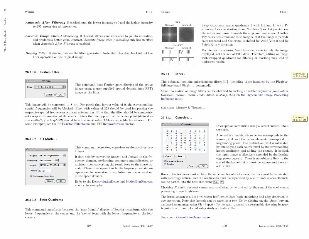
Process . FFT .

Autoscale After Filtering If checked, puts the lowest intensity to 0 and the highest intensityto 255, preserving all intensities.

Saturate Image when Autoscaling If checked, allows some intensities to go into saturation,and produces a better visual contrast. Saturate Image when Autoscaling only has an effectwhen Autoscale After Filtering is enabled.

Display Filter If checked, shows the filter generated. Note that this disables Undo of thefilter operation on the original image.

26.10.6 Custom Filter. . .

This command does Fourier space filtering of the activeimage using a user-supplied spatial domain (non-FFT)image as the filter.

This image will be converted to 8–bit. For pixels that have a value of 0, the correspondingspatial frequencies will be blocked. Pixel with values of 255 should be used for passing therespective spatial frequencies without attenuation. Note that the filter should be symmetricwith respect to inversion of the center: Points that are opposite of the center point (defined asx = width/2, y = height/2) should have the same value. Otherwise, artifacts can occur. Forsome examples, see the FFTCustomFilterDemo and FFTRemoveStreaks macros.

26.10.7 FD Math. . .

This command correlates, convolves or deconvolves twoimages.

It does this by converting Image1 and Image2 to the fre-quency domain, performing conjugate multiplication ordivision, then converting the result back to the space do-main. These three operations in the frequency domain areequivalent to correlation, convolution and deconvolutionin the space domain.

Refer to the DeconvolutionDemo and MotionBlurRemovalmacros for examples.

26.10.8 Swap Quadrants

This command transforms between the ‘user friendly’ display of Fourier transforms with thelowest frequencies at the center and the ‘native’ form with the lowest frequencies at the fourcorners.


Process . Filters .

FFTOriginal Swapped

Non-FFTOriginal Swapped

Swap Quadrants swaps quadrants I with III and II with IV(counter-clockwise starting from ‘Northeast’) so that points nearthe center are moved towards the edge and vice versa. Anotherway to see this command is to imagine that the image is periodi-cally repeated and the origin is shifted by width/2 in x and byheight/2 in y direction.

For Fourier transforms, Swap Quadrants affects only the imagedisplayed, not the actual FHT data. Therefore, editing an imagewith swapped quadrants for filtering or masking may lead toundesired results.

26.11 Filters . Improvedin IJ 1.45mImprovedin IJ 1.45m

This submenu contains miscellaneous filters [30] (including those installed by the Plugins .Utilities . Install Plugin. . . command).

More information on image filters can be obtained by looking up related keywords (convolution,Gaussian, median, mean, erode, dilate, unsharp, etc.) on the Hypermedia Image ProcessingReference index.

See also: Memory & Threads. . .

26.11.1 Convolve. . . Improvedin IJ 1.45mImprovedin IJ 1.45m

Does spatial convolution using a kernel entered into atext area.

A kernel is a matrix whose center corresponds to thesource pixel and the other elements correspond toneighboring pixels. The destination pixel is calculatedby multiplying each source pixel by its correspondingkernel coefficient and adding the results. If needed,the input image is effectively extended by duplicatingedge pixels outward. There is no arbitrary limit to thesize of the kernel but it must be square and have anodd width.

Rows in the text area must all have the same number of coefficients, the rows must be terminatedwith a carriage return, and the coefficients must be separated by one or more spaces. Kernelscan be pasted into the text area using Ctrl V .

Checking Normalize Kernel causes each coefficient to be divided by the sum of the coefficients,preserving image brightness.

The kernel shown is a 9× 9 “Mexican hat”, which does both smoothing and edge detection inone operation. Note that kernels can be saved as a text file by clicking on the ‘Save’ button,displayed as an image using File . Import .Text Image. . . , scaled to a reasonable size using Image .Adjust .Size. . . and plotted using Analyze . Surface Plot. . .

See also: ConvolutionDemo macro


The

IJUser

Guid

e—

Bookle

t59

Process . Filters .

26.11.2 Gaussian Blur. . .Improvedin IJ 1.45mImprovedin IJ 1.45m

This filter uses convolution with a Gaussian function for smoothing[31].

Sigma is the radius of decay to e−0.5 (≈ 61%), i.e., the standard devi-ation (σ) of the Gaussian (this is the same as in Adobe®Photoshop®,but different from ImageJ versions till 1.38q, in which radius was2.5×σ (cf. GaussianBlur.java).

Like all ImageJ convolution operations, it assumes that out-of-image pixels have a value equalto the nearest edge pixel. This gives higher weight to edge pixels than pixels inside the image,and higher weight to corner pixels than non-corner pixels at the edge. Thus, when smoothingwith very high blur radius, the output will be dominated by the edge pixels and especially thecorner pixels (in the extreme case, with a blur radius of e.g. 1020, the image will be replaced bythe average of the four corner pixels).

For increased speed, except for small blur radii, the lines (rows or columns of the image) aredownscaled before convolution and upscaled to their original length thereafter.

See also: Accurate Gaussian Blur plugin, AnimatedGaussianBlur macro

26.11.3 Median. . .Improvedin IJ 1.45mImprovedin IJ 1.45m

Reduces noise in the active image by replacing each pixel with the median of the neighboringpixel values.

26.11.4 Mean. . .Improvedin IJ 1.45mImprovedin IJ 1.45m

Smooths the current image by replacing each pixel with the neighborhood mean.

26.11.5 Minimum. . .Improvedin IJ 1.45mImprovedin IJ 1.45m

This filter does grayscale erosion by replacing each pixel in the image with the smallest pixelvalue in that pixel’s neighborhood.

See also: Binary .Erode

26.11.6 Maximum. . .Improvedin IJ 1.45mImprovedin IJ 1.45m

This filter does grayscale dilation by replacing each pixel in the image with the largest pixelvalue in that pixel’s neighborhood.

See also: Binary .Dilate


Process . Batch .

26.11.7 Unsharp Mask. . . Improvedin IJ 1.45mImprovedin IJ 1.45m

Sharpens and enhances edges by subtracting a blurredversion of the image (the unsharp mask) from the original.

Unsharp masking subtracts a blurred copy of the imageand rescales the image to obtain the same contrast of large(low-frequency) structures as in the input image. This isequivalent to adding a high-pass filtered image and thussharpens the image.

Radius The standard deviation (σ blur radius, cf. Gaussian Blur. . . ) of the Gaussian blur thatis subtracted. Increasing the Gaussian blur radius will increase contrast.

Mask Weight Determines the strength of filtering, whereby MaskWeight = 1 would be aninfinite weight of the high-pass filtered image that is added. Increasing the Mask Weightvalue will provide additional edge enhancement.

26.11.8 Variance. . . Improvedin IJ 1.45mImprovedin IJ 1.45m

Highlights edges in the image by replacing each pixel with the neighborhood variance.

26.11.9 Show Circular Masks. . .

Generates a stack containing examples of the circular masks used by the Median. . . , Mean. . . ,Minimum. . . , Maximum. . . , and Variance. . . filters for various neighborhood sizes.

26.12 Batch .

This submenu allows the execution of commands in a series of images without manual intervention.

Batch . commands are non-recursive, i.e., they are applied to all the images of the chosen Inputfolder but not its subfolders. Nevertheless a directory hierarchy can be transversed using ImageJmacro language (cf. BatchProcessFolders macro).

Three critical aspects to keep in mind when performing batch operations that modify processedimages:

– Files can be easily overwritten since the batch processor will silently override existing fileswith the same name.

– The destination Output folder should have adequate disk space to receive the createdimages.

– In the case of non-native formats, batch operations will be influenced by the behavior ofthe reader plugin or library (cf. Non–native Formats).


The

IJUser

Guid

e—

Bookle

t60

Process . Batch .

26.12.1 Measure. . .

This command measures all the images in a user-specified folder, by running the Analyze .Measure. . . [m] command in all images of the chosen directory.

Note that measurements are performed on non thresholded images. In the case of TIFF imagessaved with active selections measurements are performed on the ROI and not the whole image.

See also: Analyze . Set Measurements. . . , Batch .Macro. . .

26.12.2 Convert. . .Improvedin IJ 1.45mImprovedin IJ 1.45m

Batch converts and/or resizes multiple imagesfrom a specified folder.

Input... Selects the source folder containingthe images to be processed.

Output... Selects the destination folder wherethe processed images will be stored.

Output Format Specifies the output format that can be set to TIFF, 8–bit TIFF, JPEG,GIF, PNG, PGM, BMP, FITS, Text Image, ZIP or Raw (cf. Image Types and Formatsand File . Save As . submenu).

Interpolation The resampling method to be used in case Scale Factor is not 1.00 (see Im-age .Size. . . and Image .Scale. . . [E]). For better results, Average when downsizing isautomatically selected when scaling down images.

Scale Factor Specifies if images should be resized (see Image .Scale. . . [E]).

26.12.3 Macro. . .Improvedin IJ 1.45mImprovedin IJ 1.45m

Runs a macro over all the images in aspecified folder. The macro is stored inthe /ImageJ/macros/batchmacro.ijm file.

Input... Selects the source folder con-taining the images to be processed.

Output... Selects the destination folderwhere the processed images will bestored.

Output Format Specifies the outputformat that can be set to TIFF, 8–bit TIFF, JPEG, GIF, PNG, PGM,BMP, FITS, Text Image, ZIP orRaw (cf. Image Types and Formatsand File . Save As . submenu).


Process . Image Calculator. . .

Add Macro Code This drop-down menu contains macro snippets that can be combined tocreate the processing macro. Other statements can be pasted from the macro recorderor ImageJ’s editor while the dialog box is opened [32]. Previously written macros canbe imported using Open. . . When editing the macro beware of any statements that mayinterfere with the normal operation of the batch processor (such as Close() or Open()calls).

Test Tests the macro on the first image of the Input . . . folder (the processed image will bedisplayed).

Open. . . Imports previously written macros.

Save. . . Saves the assembled macro.

Help Opens http://imagej.nih.gov/ij/docs/menus/file.html#raw.

See also: Plugins .Macros .Record. . . , Batch .Virtual Stack. . .

26.12.4 Virtual Stack. . .

This command, that shares the same interface of Batch .Macro. . . (cf. BatchProcesser.java),allows virtual stack manipulations. E.g., Cropping a virtual stack can be performed by executingthe following steps:

1. Open a virtual stack

2. Run Process .Batch .Virtual Stack. . .

3. Select an Output folder and Output format

4. Select ‘Crop’ from the Add Macro Code drop-down menu

5. Edit the macro code as needed and press the Test button to verify the macro

6. Click Process to create the cropped virtual stack

Note that cropped images are not loaded into memory but are saved to disk as they are cropped(see Virtual Stacks).

26.13 Image Calculator. . .

Performs arithmetic and logical operations betweentwo images selected from popup menus.

Image1 or both Image1 and Image2 can be stacks.If both are stacks, they must have the same numberof slices. Image1 and Image2 do not have to bethe same data type or the same size.

With 32–bit (float) images, pixels resulting fromdivision by zero are set to Infinity, or to NaN(Not a Number) if a zero pixel is divided by zero.The divide-by-zero value can be redefined in Edit .Options .Misc. . .

Operation Selects one of the thirteen available op-erators (see Image Calculator. . . operations).


The

IJUser

Guid

e—

Bookle

t61

Process . Subtract Background. . .

Create New Window If checked, a new image or stack will be created to hold the result.Otherwise, the result of the operation replaces some or all of Image1.

32–bit (float) Result If checked, the source images will be converted to 32–bit floating pointbefore the specified operation is performed.

Help Opens http://imagej.nih.gov/ij/docs/menus/process.html#calculator.

Image Calculator. . . operations. On these examples source and destination images (8–bit grayscale)are displayed with inverted LUTs (White= 0; Black= 255) (cf. Lookup Tables . submenu). Note thatcalculations between images can also be performed using copy and paste and the Edit .Paste Control. . .command.

Source image (img1): Destination image (img2):

Operator Result Operator Result

Add: Min:img1 = img1 + img2 img1 = min(img1, img2)

Subtract: Max:img1 = img1− img2 img1 = max(img1, img2)

Multiply: Average:img1 = img1× img2 img1 = (img1 + img2)/2

Divide: Difference:img1 = img1÷ img2 img1 = |img1− img2|

AND: Copy:img1 = img1 ∧ img2 img1 = img2

OR: Transparent–zeroimg1 = img1 ∨ img2

XOR:img1 = img1⊕ img2

26.14 Subtract Background. . .

Removes smooth continuous backgrounds from gels andother images.

Based on the ‘rolling ball’ algorithm by Stanley Sternberg(see Sternberg S, Biomedical image processing, IEEE Com-puter, Jan 1983). Imagine a 3D surface with the pixel valuesof the image being the height, then a ball rolling over theback side of the surface creates the background. If SlidingParaboloid is checked, the command will use a more robustimplementation of the algorithm that uses an approximationof a paraboloid of rotation instead of a ball.


Process . Subtract Background. . .

Original Image Corrected Image

Process . Subtract Background. . . command. This command uses a ‘sliding paraboloid’ or a legacy‘rolling ball’ algorithm that can be used to correct for uneven illuminated background as shown in theprofiles (Analyze .Plot Profile [k]) below each image. The radius should be set to at least the size of thelargest object that is not part of the background.

Rolling Ball Radius The radius of curvature of the paraboloid. As a rule of thumb, for 8–bitor RGB images it should be at least as large as the radius of the largest object in the imagethat is not part of the background. Larger values will also work unless the background ofthe image is too uneven. For 16–bit and 32–bit images with pixel value ranges differentfrom 0–255, the radius should be inversely proportional to the pixel value range (e.g., for16–bit images (pixel values 0–65535), typical values of the radius are around 0.2 to 5).

Light Background Allows the processing of images with bright background and dark objects.

Separate Colors (RGB images only) If unchecked, the operation will only affect the brightness,leaving the hue and saturation untouched.

Create Background (Don’t Subtract) If checked, the output is not the image with thebackground subtracted but rather the background itself. This option is useful for examiningthe background created (in conjunction with the Preview option). Create Background canbe also used for custom background subtraction algorithms where the image is duplicatedand filtered (e.g. removing ‘holes’ in the background) before creating the background andfinally subtracting it with Process . Image Calculator. . .

Sliding Paraboloid If checked, the ‘rolling ball’ is replaced by a paraboloid that has thesame curvature at the apex as a ball of that radius. This option allows any value ofthe radius> 0.0001 (The ‘rolling ball’ algorithm requires a radius of at least 1). The‘sliding paraboloid’ typically produces more reliable corrections since the ‘rolling ball’,a legacy algorithm, is prone to edge artifacts. E.g., to reduce the computing time the‘rolling ball’ algorithm downscales the image in a way that is not really consistent. The‘sliding paraboloid’ algorithm does not use downscaling and thus produces no downscalingartifacts. Nevertheless, the ‘sliding paraboloid’ is also an approximation, since it does notreally use a paraboloid (an exact implementation would require a great computing effort)but it rather slides parabolae in different directions over the image.

Disable Smoothing For calculating the background (‘rolling the ball’), images are maximum-filtered (3×3 pixels) to remove outliers such as dust and then smoothed to reduce noise(average over (3×3 pixels). With Disable Smoothing checked, the unmodified image dataare used for creating the background. Check this option to make sure that the image dataafter subtraction will never be below the background.


The

IJUser

Guid

e—

Bookle

t62

Process . Repeat Command [R]

Help Opens http://imagej.nih.gov/ij/docs/menus/process.html#background.

See also: How to correct background illumination in brightfield microscopy by G. Landini,Auto Local Threshold, Background subtractor, Rolling Ball Background Subtraction(the plugin that implemented this command in versions up to 1.39e)

26.15 Repeat Command [R]

Reruns the previous command. The Edit .Undo and File .Open commands are skipped.

See also: Undo and Redo


Analyze .

27 Analyze .

This menu contains commands related to statistical measurements on image data, profile andhistogram plotting and plugins related to image analysis.

27.1 Measure. . . [m]

Based on the selection type, calculates and displays on the Results Table either area statistics,line lengths and angles, or point coordinates. Performed measurements can be specified in theSet Measurements. . . dialog box.

Area statistics are calculated for the complete image if there is no selection or for a selectedsubregion defined by one of the first four tools in the toolbar (cf. Area Selection Tools). For linearselections (Straight, Segmented and Freehand lines, cf. Line Selection Tools) length and angle(straight lines only) are also calculated. For Point selections (cf. Point Tool and Multi-pointTool), the X and Y coordinates are recorded. Note that Measure. . . [m] will paint (invasively) amark over the measured point in foreground color unless Mark Width in the Point Tool optionsdialog box is set to zero (cf. Point Tool).

With RGB images, results are calculated using brightness values. RGB pixels are convertedto brightness values using the formula value = (red + green + blue)/3 or value = 0.299 ×red+ 0.587× green+ 0.114× blue if Weighted RGB Conversions is checked in Edit .Options .Conversions. . . .

Intensity statistics (Mean, Modal, Median, Min. & Max. Gray Value, Standard Deviation andIntegrated Density) can be performed on area, line and multi-point selections.

With area selections, the following parameters can be recorded: Area, Center of Mass, Centroid,Perimeter, Bounding Rectangle, Shape Descriptors, Fitted Ellipse, Feret’s Diameter, Skewness,Kurtosis and Area Fraction.

With line selections, the following parameters can be recorded: Length, Angle (straight linesonly), and Bounding Rectangle. The mean, standard deviation, etc. are calculated from thevalues of the pixels along the line.

See also: Results Table, Analyze Particles. . . , Summarize, Distribution. . . , Set Measurements. . . ,Batch .Measure. . .

27.2 Analyze Particles. . .

This command counts and measures objects inbinary or thresholded images (Image .Adjust .Threshold. . . [T] or Color Threshold. . . ). Anal-ysis is performed on the existing area selectionor on the entire image if no selection is present.

It works by scanning the image or selectionuntil it finds the edge of an object. It then out-lines the object using the Wand Tool, measuresit using the Measure. . . [m] command, fills it tomake it invisible, then resumes scanning untilit reaches the end of the image or selection.Press Esc to abort this process.


The

IJUser

Guid

e—

Bookle

t63

Analyze . Analyze Particles. . .

Original (thresholded) Exclude on Edges Include Holes Size: 0–50 Circ.: 0.5–1.0

Size: 0–∞ Circ.: 0.0–0.5 Size: 0–∞ Circ.: 0.3–0.5 Size: 0–∞ Circ.: 0.0–0.3 Size: 50–∞ Circ.: 0.5–1.0

Particle Analyzer (Analyze .Analyze Particles. . . ). Features of thresholded images can be extractedby specifying suitable Size and Circularity ranges and/or by choosing if particles should be traced bytheir outer edge or by flood filling (Include Holes checkbox).

Size Particles with size (area) outside the range specified in this field are ignored. Values mayrange between 0 and ‘Infinity’. For spatial scaled images (cf. Set Scale. . . ) values areexpressed in physical size square units or in pixels if Pixel Units is checked. Enter a singlevalue and particles smaller than that value will be ignored.

Circularity Particles with size circularity values outside the range specified in this field are alsoignored. Circularity (4π × [Area]

[Perimeter]2, cf. Set Measurements. . . ) ranges from 0 (infinitely

elongated polygon) to 1 (perfect circle).

Show This drop-down menu specifies which image (or overlay) should ImageJ display afterthe analysis (see Display options of Particle Analyzer). Note that with IJ 1.44e andlater, the particle analyzer will display a blank image when the count of detected particlesis zero and Show is not Nothing. The font size and line width used can be change ina macro by using call("ij.plugin.filter.ParticleAnalyzer.setFontSize", size);and call("ij.plugin.filter.ParticleAnalyzer.setLineWidth", width); in a macroor ParticleAnalyzer.setFontSize(size); ParticleAnalyzer.setLineWidth(width);in a script or plugin.

Nothing Neither images nor overlays will be displayed.

Outlines 8–bit image containing numbered outlines of the measured particles (gray levels:Outlines : 0; Labels : 1; Background : 255). If In situ Show is checked, the original imagewill be replaced by this image.

Bare Outlines 8–bit image containing simple outlines of the measured particles withoutlabels (graylevels: Outlines: 0; Background : 255). If In situ Show is checked, theoriginal image will be replaced by this image.


Analyze . Analyze Particles. . .

Masks 8–bit binary image containing filled outlines of the measured particles (gray levels:Masks: 0; Background : 255). If In situ Show is checked, the original image will bereplaced by this image.

Ellipses 8–bit binary image containing the best fit ellipse (cf. Edit . Selection .Fit Ellipse)of each measured particle (gray levels: Ellipses: 0; Background : 255). If In situ Showis checked, the original image will be replaced by this image.

Count Masks 16–bit image containing filled outlines of the measured particles paintedwith a grayscale value corresponding to the particle number. If In situ Show ischecked, the original image will be replaced by this image.

Overlay Outlines Displays outlines of the measured particles in the image overlay,removing previously added overlays will be removed.

Overlay Masks Displays filled outlines of the measured particles in the image overlay,removing previously added overlays will be removed.

Display Results If checked, the measurements for each particle will be displayed in the ResultsTable.

Clear Results If checked, any previous measurements listed in the Results Table will becleared.

Summarize If checked, the particle count, total particle area, average particle size, areafraction and the mean of all parameters listed in the Set Measurements. . . dialog box willbe displayed in a separate Summary table. Note that while single images ‘Summaries’are output to the same Summary table, stack Summaries are printed in dedicated tables(named Summary of [stack title]). Also, note that descriptive statistics on Resultsmeasurements can be obtained at any time using the Summarize command.

Add to Manager If checked, the measured particles will be added to the ROI Manager. . .

Exclude on Edges If checked, particles touching the edge of the image (or selection) will beignored.

Include Holes If checked, interior holes will be included. Disable this option to excludeinterior holes and to measure particles enclosed by other particles. When this option isenabled, ImageJ finds the extent of each particle by tracing the outer edge. When it isdisabled, ImageJ finds the extent by flood filling.

Record Starts This option allows plugins and macros to recreate particle outlines using thedoWand(x,y) macro function. The CircularParticles macro demonstrates how to use thisfeature.

In situ Show If checked, the original image will be replaced by the binary mask specified inthe Show drop-down menu. Note that this option does not apply to Overlay Outlinesand Overlay Masks that are always displayed as non-destructive image overlays on themeasured image.

Help Opens http://imagej.nih.gov/ij/docs/menus/analyze.html#ap.

See also: Particle Remover plugin, 4/8–Connected Particle Analysis


The

IJUser

Guid

e—

Bookle

t64

Analyze . Summarize

Original (thresholded) Outlines Bare Outlines Masks

Ellipses Count Masks Overlay Outlines Overlay Masks

Display options of Particle Analyzer (Analyze .Analyze Particles. . . ), IJ 1.44l.

27.3 Summarize

For each column in the Results Table, calculates and displays the mean, standard deviation,minimum and maximum of the values in that column. This command is also available byright-clicking on the Results Table.

See also: Analyze Particles. . . , Distribution. . .

27.4 Distribution. . .

Produces a relative frequency histogram from the data of a chosen column of the Results table[33].

Use the List or Copy buttons to save the histogram data. Mouse over the histogram bars to readthe counts for each bin on the window’s lower right corner. Analyze .Histogram [h] describes inmore detail ImageJ’s histogram window.

This command is also available by right-clicking on the Results Table.


Analyze . Label

Parameter Specifies the parameter inthe Results Table to be analyzed.

Data points The number of rows thatwill be analyzed (informative).

Automatic binning If checked, ImageJwill use the method described byDavid Scott to assess the opti-mal histogram bin width (see ScottDW, Optimal and data-based his-tograms. Biometrika, 66(3):605–610,Jan 1979). If unchecked, the numberof bins can be set with Specify binsand the starting and ending limits ofthe histogram with range.

See also: Distribution Plotter, a macro that plots relative and cumulative frequencies on adouble Y-axis graph

27.5 Label

This command labels the active selection with the current measurement counter value, i.e.,the number of rows present in the Results Table. Selection outline and label (at the selectioncentroid) are drawn invasively using current foreground/background colors. As for Edit .Draw[d], Use the Edit .Options . Line Width. . . command, or double click on the line tool, to changethe width of selection’s outline.

Selections can be labelled if they were previously analyzed (Analyze Particles. . . or Measure. . .[m] commands) and the parameter Centroid (cf. Set Measurements. . . ) extracted in the Resultstable.

See also: Color Picker, XVII Embedding Color Annotations in Grayscale Images

27.6 Clear Results

Erases the results table and resets the measurement counter. This command is also available byright-clicking on the Results Table.

27.7 Set Measurements. . . Improvedin IJ 1.45mImprovedin IJ 1.45m

Use this dialog box to specify which measurements are recorded by Analyze .Measure. . . [m],ROI Manager’s Measure command (cf. ROI Manager. . . ) and Analyze .Analyze Particles. . .Measurements are performed on the current selection, the entire active image if no selection ispresent. For thresholded images, measurements can be restricted to highlighted pixels if Limitto Threshold is checked.

This command is also available by right-clicking on the Results Table.

The dialog contains two groups of checkboxes: The first group controls the type of measurementsthat are printed to the Results table. The second group controls measurement settings.


The

IJUser

Guid

e—

Bookle

t65

Analyze . Set Measurements. . .

The eighteen checkboxes of the first group are:

Area Area of selection in square pixels or in cali-brated square units (e.g., mm2, µm2, etc.) ifAnalyze .Set Scale. . . was used to spatiallycalibrate the image.

Mean gray value Average gray value within theselection. This is the sum of the gray val-ues of all the pixels in the selection dividedby the number of pixels. Reported in cali-brated units (e.g., optical density) if Analyze .Calibrate. . . was used to calibrate the im-age. For RGB images, the mean is calculatedby converting each pixel to grayscale usingthe formula gray = (red+ green+ blue)/3 orgray = 0.299×red+0.587×green+0.114×blueif Weighted RGB Conversions is checked inEdit .Options .Conversions. . .

Standard deviation Standard deviation of the gray values used to generate the mean grayvalue. Uses the Results Table heading StdDev.

Modal gray value Most frequently occurring gray value within the selection. Corresponds tothe highest peak in the histogram. Uses the heading Mode.

Min & max gray level Minimum and maximum gray values within the selection.

Centroid The center point of the selection. This is the average of the x and y coordinates ofall of the pixels in the image or selection. Uses the X and Y headings.

Center of mass This is the brightness-weighted average of the x and y coordinates all pixelsin the image or selection. Uses the XM and YM headings. These coordinates are thefirst order spatial moments.

Perimeter The length of the outside boundary of the selection. Uses the heading Perim.. WithIJ 1.44f and later, the perimeter of a composite selection is calculated by decomposing itinto individual selections. Note that the composite perimeter and the sum of the individualperimeters may be different due to use of different calculation methods.

Bounding rectangle The smallest rectangle enclosing the selection. Uses the headings BX,BY, Width and Height, where BX and BY are the coordinates of the upper left cornerof the rectangle.

Fit ellipse Fits an ellipse to the selection. Uses the headings Major, Minor and Angle.Major and Minor are the primary and secondary axis of the best fitting ellipse. Angleis the angle between the primary axis and a line parallel to the X-axis of the image. Thecoordinates of the center of the ellipse are displayed as X and Y if Centroid is checked.Note that ImageJ cannot calculate the major and minor axis lengths if Pixel Aspect Ratioin the Analyze .Set Scale. . . dialog is not 1.0. There are several ways to view the fittedellipse:

1. The Edit . Selection .Fit Ellipse command replaces an area selection with the best fitellipse.


Analyze . Set Measurements. . .

2. The DrawEllipse macro draws (destructively) the best fit ellipse and the major andminor axis.

3. Select Ellipses from the Show: drop-down menu in the particle analyzer (Analyze .Analyze Particles. . . ) and it will draw the ellipse for each particle in a separatewindow.

Shape descriptors Calculates and displays the following shape descriptors:

Circularity 4π × [Area][Perimeter]2

with a value of 1.0 indicating a perfect circle. As the valueapproaches 0.0, it indicates an increasingly elongated shape. Values may not be validfor very small particles. Uses the heading Circ.

Aspect ratio The aspect ratio of the particle’s fitted ellipse, i.e., [Major Axis][Minor Axis] . If Fit

Ellipse is selected the Major and Minor axis are displayed. Uses the heading AR.Roundness 4× [Area]

π×[Major axis]2or the inverse of Aspect Ratio. Uses the heading Round.

Solidity [Area][Convex area] ; Note that the Edit . Selection .Convex Hull command makes an area

selection convex.

Feret’s diameter The longest distance between any two points along the selection boundary, Improvedin IJ 1.45mImprovedin IJ 1.45malso known as maximum caliper. Uses the heading Feret. The angle (0–180 degrees) of

the Feret’s diameter is displayed as FeretAngle, as well as the minimum caliper diameter(MinFeret). The length of the object’s projection in the X (FeretX) and Y (FeretY)direction is also displayed (see also Feret’s Diameter macro and Chamfer distances andGeodesic diameters plugin).

Integrated density The sum of the values of the pixels in the image or selection. This isequivalent to the product of Area and Mean Gray Value. With IJ 1.44c and later, Rawintegrated density (sum of pixel values) is displayed under the heading RawIntDenwhen Integrated density is enabled. The Dot Blot Analysis tutorial demonstrates howto use this option to analyze a dot blot assay.

Median The median value of the pixels in the image or selection.

Skewness The third order moment about the mean. The documentation for the MomentCalculator plugin explains how to interpret spatial moments. Uses the heading Skew.

Kurtosis The fourth order moment about the mean. Uses the heading Kurt.

Area fraction For thresholded images is the percentage of pixels in the image or selection thathave been highlighted in red using Image .Adjust .Threshold. . . [T]. For non-thresholdedimages is the percentage of non-zero pixels. Uses the heading %Area.

Stack position The position (slice, channel and frame) in the stack or hyperstack of theselection. Uses the headings Slice, Ch and Frame.

n.b.: For line selections the heading Length is created. For straight line selections, Angle isrecorded even if Fit Ellipse is unchecked. Also, note that measurements that do notapply to certain selection types may be listed as NaN, Infinity or −Infinity.

The second part of the dialog controls measurement settings:

Limit to threshold If checked, only thresholded pixels are included in measurement calcula-tions. Use Image .Adjust .Threshold. . . [T] to set the threshold limits. This setting affectsonly thresholded images (see Settings and Preferences).


The

IJUser

Guid

e—

Bookle

t66

Analyze . Set Scale. . .

Display label If checked, the image name and slice number (for stacks) are recorded in thefirst column of the Results Table, e.g., mri-stack.tif:9. For renamed selections (Edit .Selection .Properties. . . [y]) or selections measured via ROI Manager’s measure com-mand (see ROI Manager. . . ), the selection label is appended, e.g., blobs.gif:0339-0163 orblobs.gif:mySelection.

Invert Y coordinates If checked, the XY origin is assumed to be the lower left corner of theimage window instead of the upper left corner (see also Image .Properties. . . [P]).

Scientific notation If checked, measurements are displayed in scientific notation, e.g., 1.48E2.

Add to Overlay If checked, measured ROIs are automatically added to the image overlay.New inIJ 1.45mNew inIJ 1.45m

Each measured selection will be displayed with an accompanying numeric label, matchingits row in the Results Table. Selections color can be changed in Edit .Options .Colors. . .or by double clicking on the Point Tool. The numeric label is defined by the “Show All”color in ROI Manager’s More�Options. . . widget.

Redirect to The image selected from this popup menu will be used as the target for statisticalcalculations done by Analyze .Measure. . . [m] and Analyze .Analyze Particles. . . commands.This feature allows you to outline a structure on one image and measure the intensity ofthe corresponding region in another image.

Decimal places This is the number of digits to the right of the decimal point in real numbersdisplayed in the Results Table and in Histogram windows (Analyze .Histogram [h]).

27.8 Set Scale. . .

Use this dialog to define the spatial scale of the active imageso measurement results can be presented in calibrated units,such as mm or µm.

Before using this command, use the straight line selection toolto make a line selection that corresponds to a known distance.Then, bring up the Set Scale. . . dialog, enter the KnownDistance and unit of measurement, then click ‘OK’.

ImageJ will have automatically filled in the Distance in Pixelsfield based on the length of the line selection.

Setting Pixel Aspect Ratio to a value other than 1.0 enables support for different horizontal andvertical spatial scales, e.g., 100 pixels/cm horizontally and 95 pixels/cm vertically. To set thePixel Aspect Ratio:

1. Measure the width and height (in pixels) of a digitized object with a known 1:1 aspectratio.

2. Enter the measured width (in pixels) in Distance in Pixels. Enter the known width inKnown Distance.

3. Calculate the aspect ratio by dividing the width by the height and enter it in Pixel AspectRatio

When Global is checked, the scale defined in this dialog is used for all opened images during thecurrent session instead of just the active image, see XXII Global Calibrations.


Analyze . Calibrate. . .

Click to Remove Scale resets Distance in Pixels field and Know Distance to zero and the Unitof Length to ‘pixel’.

See also: Three tutorials showing how to use this command: Examples of Image AnalysisUsing ImageJ by Larry Reinking, Measuring DNA Contour Lengths and SpatialCalibration (Fiji). The Copy_Pixel_Size plugin

27.9 Calibrate. . .

Use this dialog box to calibrate an image to a set of density standards, for example radioactiveisotope standards or a calibrated optical density step tablet.

Note that to create a calibration curve, the left column must contain a list of measured meanpixel values and the right column must contain the same number of calibration standard values.

The ImageJ web site has a tutorial on Optical Density Calibration explaining how to calibratean image to an optical density step tablet.

1. Before using this command, use Analyze .Clear Results to reset the measurement counterand use one of the selection tools and Analyze .Measure. . . [m] to record the mean grayvalue of each of the standards.

2. When finished making the measurements, select Analyze .Curve Fitting. . . to display theCalibrate dialog box. To calibrate the image, enter the known standard values in the rightcolumn. The left column will be already populated with the measured mean gray values.Select a curve fitting method from the popup menu, enter the unit of measurement, andclick ‘OK’. ImageJ will then display the calibration function on a separate window.

3. If the calibration function is not satisfactory, bring up the Calibrate. . . dialog box againand select a different curve fitting method.

In addition to the fourteen functions that can be chosen from the drop-down menu (describedin Curve Fitting. . . ) two other functions are available that do not require any measurement ofOD standards:


The

IJUser

Guid

e—

Bookle

t67

Analyze . Histogram [h]

Uncalibrated OD Causes ImageJ to convert gray values from 8–bit images to uncalibratedoptical density values using the function Unc. OD = log10(255/Pixel value).

Pixel Inverter Linear function defined by Inverted pixel = Bit-depth − 1−Pixel value, withBit-depth being 255 for 8–bit images or 65535 for 16–bit images.

See also: Global Calibrations, Image Types and Formats, Curve Fitting. . .

XXII Global Calibrations

Calibration settings related to spatial (pixel width, height and voxel depth), temporal (frameinterval) and luminance (brightness) information can be set globally, i.e., can be applied to allimages opened during the current session instead of just the active image. The Global flag canbe set in three dialog prompts:

1. Image .Properties. . . [P] (pixel width, height, voxel depth, frame interval)

2. Analyze . Set Scale. . . (pixel width and height)

3. Analyze .Calibrate. . . (pixel intensity)

Once Global calibration is set, a ‘(G)’ is displayed in all imagetitles until ImageJ is closed. A warning message is displayedwhen a calibrated image with conflicting calibration is openedand the Global option is enabled.

Choose Disable Global Calibration to stop using global set-tings or Disable these Messages to keep respecting globalsettings, ignoring the calibration of the newly open image.

27.10 Histogram [h]1

Calculates and displays a histogram of thedistribution of gray values in the active imageor selection.

The X-axis represents the possible gray val-ues and the Y-axis shows the number of pix-els found for each gray value. The horizontalLUT bar below the X-axis is scaled to reflectthe display range of the image [34]. The totalpixel Count is also calculated and displayed,as well as the Mean, standard deviation (Std-Dev), minimum (Min), maximum (Max ) andmodal (Mode) gray value.

Use the List or Copy buttons to save the histogram data. Click on Log to display a log-scaledversion of the histogram (overlaid in gray).

1This shortcut is shown on Windows and Linux but not on Mac OSX as it conflicts with the system wide ‘Hide’shortcut. However, the H shortcut (without holding down Cmd ) does work on OSX.


Analyze . Plot Profile [k]

Value /Count pairs (i.e., grayscale value corresponding to the X-axis cursor position / the numberof pixels that have that intensity) are displayed on the bottom right while mousing over thehistogram window.

With RGB images, the histogram is calculated by converting each pixel to grayscale using theformula gray = (red+ green+ blue)/3 or gray = 0.299× red+ 0.587× green+ 0.114× blue ifWeighted RGB Conversions is checked in Edit .Options .Conversions. . . . With 16–bit images,the range of gray values between the Min and Max values is divided into 256 bins. With 32–bitimages, the number of bins is specified in the depicted dialog box.

With any image type, an options dialog can be called with Alt H orby holding Alt while clicking on Analyze .Histogram [h].

Bins Specifies the number of bins.

Use min/max If checked, the X-axis range is determined by theminimum and maximum values in the image or selection. Ifunchecked, X Min and X Max values can be or specified to fixthe X-axis range.

Y Max Fixes the Y-axis range. Type ‘Auto’ to have the rangedetermined by the largest bin count.

The getHistogram() and Plot.getValues() macro functions can be used to get the ‘value’and ‘Count’ data displayed when you click the List button (cf. (6) Obtaining Histogram Lists).

(6) Obtaining Histogram Lists1 // 1. Single images:2 run("Blobs (25K)");3 getHistogram(values , counts , 256);4 for (i=0; i<values.length; i++)5 print(values[i], counts[i]);6

7 // 2. Entire stacks:8 run("T1 Head (2.4M , 16-bits)");9 run("Histogram", "stack");

10 Plot.getValues(values , counts);11 for (i=0; i<values.length; i++)12 print(values[i], counts[i]);

27.11 Plot Profile [k] Improvedin IJ 1.45mImprovedin IJ 1.45m

Displays a two-dimensional graph of the in-tensities of pixels along a line or rectangularselection. The X-axis represents distancealong the line and the Y-axis is the pixelintensity. NaNs values in 32–bit images (seeImage Types and Formats) are ignored.

For rectangular selections or line selectionswider than one pixel, displays a ‘columnaverage plot’, where the X-axis representsthe horizontal distance through the selectionand the Y-axis the vertically averaged pixelintensity.


The

IJUser

Guid

e—

Bookle

t68

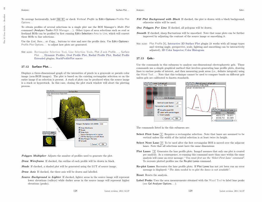
Analyze . Surface Plot. . .

To average horizontally, hold Alt K or check Vertical Profile in Edit .Options .Profile PlotOptions. . .

To obtain profiles of several selections in a single plot use the ROI Manager’s Multi Plotcommand (Analyze .Tools .ROI Manager. . . ). Other types of area selections such as oval orfreehand ROIs can be profiled by first running Edit . Selection .Area to Line, which will convertthese ROIs to line selections.

Use the List, Save... or Copy... buttons to view and save the profile data. Use Edit .Options .Profile Plot Options. . . to adjust how plots are generated.

See also: Rectangular Selection Tool, Line Selection Tools, Plot Z-axis Profile. . . , SurfacePlot. . . , Dynamic Profiler, Oval Profile Plot, Radial Profile Plot, Radial ProfileExtended plugins, StackProfilePlot macro

27.12 Surface Plot. . .

Displays a three-dimensional graph of the intensities of pixels in a grayscale or pseudo colorimage (non-RGB images). The plot is based on the existing rectangular selection or on theentire image if no selection is present. A stack of plots can be produced when the source imageis a stack or hyperstack. In this case, closing the plot stack window will abort the plottingprocess.

Polygon Multiplier Adjusts the number of profiles used to generate the plot.

Draw Wireframe If checked, the outline of each profile will be drawn in black.

Shade If checked, a shaded plot will be generated using the LUT of source image.

Draw Axis If checked, the three axis will be drawn and labelled.

Source Background is Lighter If checked, lighter areas in the source image will representlower elevations (valleys) while darker areas in the source image will represent higherelevations (peaks).


Analyze . Gels .

Fill Plot Background with Black If checked, the plot is drawn with a black background,otherwise white will be used.

One Polygon Per Line If checked, all polygons will be drawn.

Smooth If checked, sharp fluctuations will be smoothed. Note that some plots can be furtherimproved by adjusting the contrast of the source image or smoothing it.

See also: Plot Profile [k], Interactive 3D Surface Plot plugin (it works with all image typesand viewing angle, perspective, scale, lighting and smoothing can be interactivelyadjusted), 3D Color Inspector/Color Histogram

27.13 Gels .

Use the commands in this submenu to analyze one-dimensional electrophoretic gels. Thesecommands use a simple graphical method that involves generating lane profile plots, drawinglines to enclose peaks of interest, and then measuring peak areas (i.e., definite integrals) usingthe Wand Tool. . . . Note that this technique cannot be used to compare bands on different gelsunless gels are calibrated to known standards.

The commands listed in the this submenu are:

Select First Lane 1 Requires a rectangular selection. Note that lanes are assumed to bevertical unless the width of the initial selection is at least twice its height.

Select Next Lane 2 To be used after the first rectangular ROI is moved over the adjacentlanes. Note that all selections must have the same dimensions.

Plot Lanes 3 Generates the lane profile plots. ImageJ assumes that only one plot is createdper analysis. As a consequence, re-running this command more than once within the sameanalysis will cause an error message: “You must first use the ‘Select First Lane’ command ”.To recreate plotted profiles use the Re-plot Lanes command.

Re-plot Lanes Recreates the lane profile plots. If Plot Lanes has not yet been run an errormessage is displayed: “The data needed to re-plot the lanes is not available”.

Reset Resets the analysis.

Label Peaks Uses the area measurements obtained with the Wand Tool to label lane peaks(see Gel Analyzer Options. . . ).


The

IJUser

Guid

e—

Bookle

t69

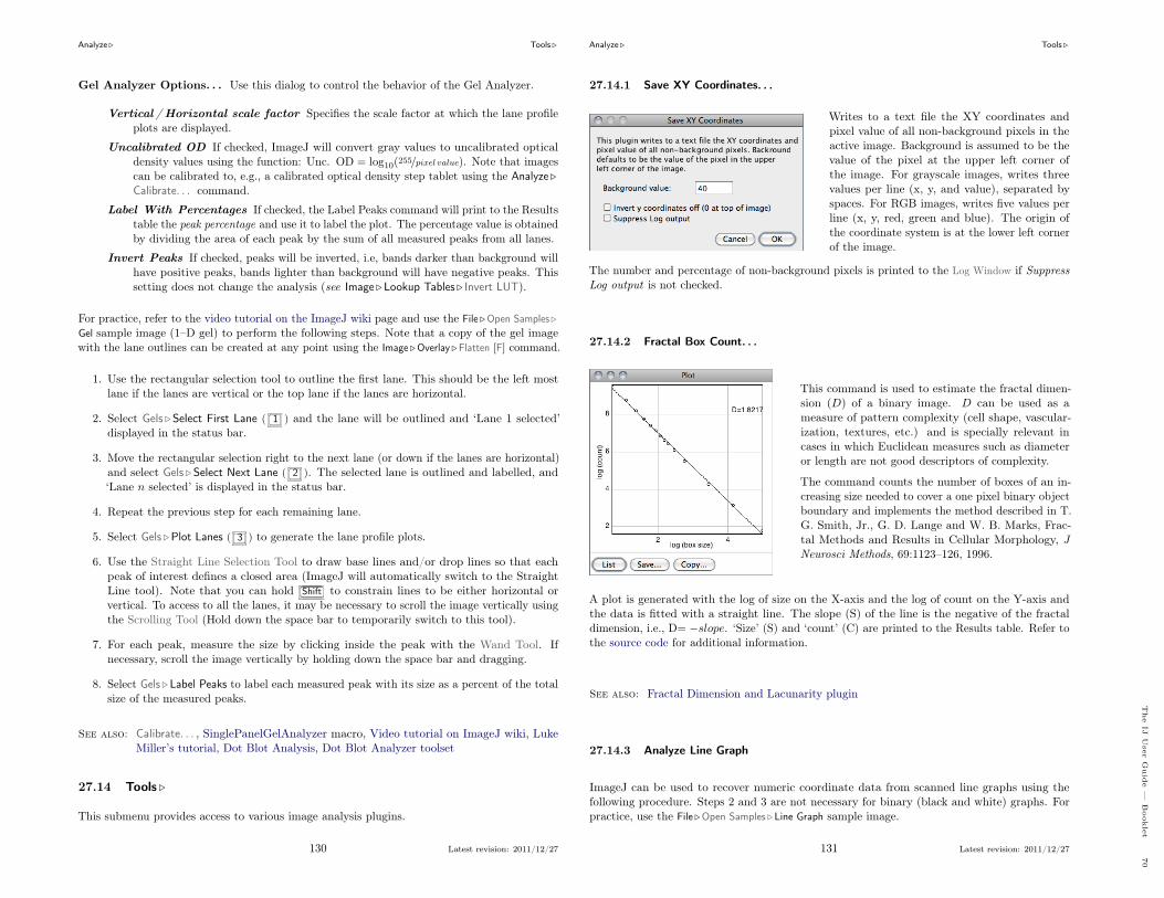
Analyze . Tools .

Gel Analyzer Options. . . Use this dialog to control the behavior of the Gel Analyzer.

Vertical /Horizontal scale factor Specifies the scale factor at which the lane profileplots are displayed.

Uncalibrated OD If checked, ImageJ will convert gray values to uncalibrated opticaldensity values using the function: Unc. OD = log10(255/pixel value). Note that imagescan be calibrated to, e.g., a calibrated optical density step tablet using the Analyze .Calibrate. . . command.

Label With Percentages If checked, the Label Peaks command will print to the Resultstable the peak percentage and use it to label the plot. The percentage value is obtainedby dividing the area of each peak by the sum of all measured peaks from all lanes.

Invert Peaks If checked, peaks will be inverted, i.e, bands darker than background willhave positive peaks, bands lighter than background will have negative peaks. Thissetting does not change the analysis (see Image . Lookup Tables . Invert LUT).

For practice, refer to the video tutorial on the ImageJ wiki page and use the File .Open Samples .Gel sample image (1–D gel) to perform the following steps. Note that a copy of the gel imagewith the lane outlines can be created at any point using the Image .Overlay .Flatten [F] command.

1. Use the rectangular selection tool to outline the first lane. This should be the left mostlane if the lanes are vertical or the top lane if the lanes are horizontal.

2. Select Gels .Select First Lane ( 1 ) and the lane will be outlined and ‘Lane 1 selected’displayed in the status bar.

3. Move the rectangular selection right to the next lane (or down if the lanes are horizontal)and select Gels .Select Next Lane ( 2 ). The selected lane is outlined and labelled, and‘Lane n selected’ is displayed in the status bar.

4. Repeat the previous step for each remaining lane.

5. Select Gels .Plot Lanes ( 3 ) to generate the lane profile plots.

6. Use the Straight Line Selection Tool to draw base lines and/or drop lines so that eachpeak of interest defines a closed area (ImageJ will automatically switch to the StraightLine tool). Note that you can hold Shift to constrain lines to be either horizontal orvertical. To access to all the lanes, it may be necessary to scroll the image vertically usingthe Scrolling Tool (Hold down the space bar to temporarily switch to this tool).

7. For each peak, measure the size by clicking inside the peak with the Wand Tool. Ifnecessary, scroll the image vertically by holding down the space bar and dragging.

8. Select Gels . Label Peaks to label each measured peak with its size as a percent of the totalsize of the measured peaks.

See also: Calibrate. . . , SinglePanelGelAnalyzer macro, Video tutorial on ImageJ wiki, LukeMiller’s tutorial, Dot Blot Analysis, Dot Blot Analyzer toolset

27.14 Tools .

This submenu provides access to various image analysis plugins.


Analyze . Tools .

27.14.1 Save XY Coordinates. . .

Writes to a text file the XY coordinates andpixel value of all non-background pixels in theactive image. Background is assumed to be thevalue of the pixel at the upper left corner ofthe image. For grayscale images, writes threevalues per line (x, y, and value), separated byspaces. For RGB images, writes five values perline (x, y, red, green and blue). The origin ofthe coordinate system is at the lower left cornerof the image.

The number and percentage of non-background pixels is printed to the Log Window if SuppressLog output is not checked.

27.14.2 Fractal Box Count. . .

This command is used to estimate the fractal dimen-sion (D) of a binary image. D can be used as ameasure of pattern complexity (cell shape, vascular-ization, textures, etc.) and is specially relevant incases in which Euclidean measures such as diameteror length are not good descriptors of complexity.

The command counts the number of boxes of an in-creasing size needed to cover a one pixel binary objectboundary and implements the method described in T.G. Smith, Jr., G. D. Lange and W. B. Marks, Frac-tal Methods and Results in Cellular Morphology, JNeurosci Methods, 69:1123–126, 1996.

A plot is generated with the log of size on the X-axis and the log of count on the Y-axis andthe data is fitted with a straight line. The slope (S) of the line is the negative of the fractaldimension, i.e., D= −slope. ‘Size’ (S) and ‘count’ (C) are printed to the Results table. Refer tothe source code for additional information.

See also: Fractal Dimension and Lacunarity plugin

27.14.3 Analyze Line Graph

ImageJ can be used to recover numeric coordinate data from scanned line graphs using thefollowing procedure. Steps 2 and 3 are not necessary for binary (black and white) graphs. Forpractice, use the File .Open Samples . Line Graph sample image.


The

IJUser

Guid

e—

Bookle

t70

Analyze . Tools .

1. Open the image containing the graph.

2. Open the Threshold. . . [T] tool ( Shift T ). Adjust thethreshold so the graph is highlighted in red.

3. Click on Apply (make sure foreground is black andbackground is white).

4. Use the Elliptical Selection Tool as an eraser (pressBackspace to erase) to isolate a single curve (NB:background color must be white, cf. Color Picker. . .[K]).

5. Select the curve by clicking to the left of it with theWand Tool.

6. Use Edit .Clear Outside to erase everything but the curve.

7. Use Analyze .Tools .Analyze Line Graph to get the XY coordinates.

ImageJ’s curve fitter (Analyze .Tools .Curve Fitting. . . ) – ImageJ 1.44l.

27.14.4 Curve Fitting. . .

ImageJ’s curve fitter provides a very simple tool for fitting various functions to X- and Y-data.The typical usage of this command is listed below.

1. Tabular data is entered or copied in the input window or alternatively, a two column textfile is opened by clicking on the Open button. Values may be separated by spaces, tabs,commas or semicolons.

2. The function to be fit is selected from the drop-down menu. Fourteen built-in functions areavailable. User defined functions with up to six parameters are also possible by choosing*User-defined*. In this case, Formula and Fitting Options must be specified by the user.

3. Once the Fit button is pressed, ImageJ displays a graph of the data with the fitted curveas well as a log window containing information about the fit and the values of the fittedparameters if Show Settings is checked.


Analyze . Tools .

Summary of ImageJ’s CurveFitter functions. The complete documentation for the CurveFitterclass is available at http://imagej.nih.gov/ij/developer/api/ij/measure/CurveFitter.html.

Function Formula Comments

Straight Line y = a+ bx cf. Pixel Inverter (Calibrate. . . )

2nd Degree Polynomial y = a+ bx+ cx2

3rd Degree Polynomial y = a+ bx+ cx2 + dx3

4th Degree Polynomial y = a+ bx+ cx2 + dx3 + ex4

5th Degree Polynomial y = a+ bx+ cx2 + dx3 + ex4 + fx5 Via the *User-defined* option

Exponential y = a× ebx

Power y = axb

Log y = a× ln(bx)

Gamma Variate y = a× (x− b)c × e−( x−bd )

Rodboard y = d+(a−d)1+( x

c )b [35]

Exponential with Offset y = a× e−(bx) + c

Gaussian y = a+ (b− a)× e−(x−c)2

2d2 [35]

Exponential Recovery y = a× (1− e(−bx)) + c cf. FRAP_Profiler plugin

4. Click Apply to create a 32–bit copy of the current image transformed with the chosenfunction.

See also: Profile Plot Options. . . , CurveFittingDemo, RodbardSigmoidFit and PlotSigmoid-Derivatives macros

27.14.5 ROI Manager. . . Improvedin IJ 1.45mImprovedin IJ 1.45m

The ROI (Region of Interest) Manager is a tool for working with multiple selections. Theselections can be from different locations on an image, from different slices of a stack or fromdifferent images. All selection types, including points, lines and text, are supported.

Add Click Add to add the current selection to the list, or press T , the keyboard shortcut forthe Edit . Selection .Add to Manager [t] command. The ROI manager creates a three partlabel. The first part (stacks only) is the slice number, the second is the Y-coordinate ofthe selection and the third is the X-coordinate. Click on a label to restore the associatedselection to the current image. With stacks, the selection is restored to the slice it camefrom. Hold down Shift while clicking Add to ‘Add and Draw’. Hold down Alt whileclicking Add to ‘Add and Rename’.Install the ROIManagerMacros macro set and you will be able to add a selection bypressing 1 , ‘add and rename’ by pressing 2 , ‘add and draw’ by pressing 3 and ‘addand advance to the next slice’ by pressing 4 .

Update Replaces the selected ROI on the list with the current selection. With IJ 1.45 it also Improvedin IJ 1.45mImprovedin IJ 1.45mupdates the z/t-position of the ROI in stacks/hyperstacks.


The

IJUser

Guid

e—

Bookle

t71

Analyze . Tools .

More » Options…

Show All with/ without labels

Show All

Show All in Edit Mode

Deselect/Select All

X-coordinate Y-coordinate Slice number

Misc. operations via drop down menu (also available when right

clicking on list area)

The ROI Manager (Analyze .Tools .ROI Manager. . . ) – ImageJ 1.45i.

Delete Deletes the selected ROIs from the list. Deletes all the ROIs if none is selected.

Rename. . . Renames the selected ROI. The chosen string will be used as Edit Mode label ifUse ROI names as labels is checked in the More�Options. . . dialog. The selected ROIcan also be renamed using the Properties. . . button.

Measure Measures the selected ROIs, or if none is selected, all ROIs on the list. Use Analyze .Set Measurements. . . to specify the parameters to measure.

Deselect Deselects any selected ROIs on the list. Delete, Measure, More�Save. . . , andMore�Combine work with all ROIs on the list when none are selected.

Properties. . . Opens a dialog box (depicted in ROI Manager) in which is possible to assign acontour color (Stroke color) of a certain Width or a Filling color. With text selections(see Text Tool), it is also possible to specify the Font size and Justification.As explained for Edit .Selection .Properties. . . [y], selections can be either filled or con-toured, but not both. The nine default selection colors (black, blue, cyan, green, magenta,orange, red, white, yellow) can be typed textually. Any other color must be specifiedusing hex notation (see XIX Hexadecimal Color Values). If multiple ROIs have beenselected from the Manager’s list (see XXIII Selecting Multiple ROIs in the ROI Manager),properties will be applied to the specified Range of selections.

Flatten [F] Alias for Image .Overlay .Flatten [F].

ShowAll Toggles a non-destructive overlay that outlines all ROI Manager selections. If EditMode is active selections will also be labelled. In this case, click on a label (selectionnumber) in the overlay to activate the corresponding selection. That selection can thenbe moved or edited and the overlay will be dynamically updated. The color and behaviorof the Show All overlay can be changed in the More�Options. . . dialog box.

EditMode Toggles selection labels displayed by Show All. As mentioned, clicking on a labelactivates its selection allowing edit operations.

More� Displays a drop-down menu with several additional commands (this menu is alsoavailable when right-clicking on the ROI Manager’s list area):


Analyze . Tools .

Open. . . Opens a .roi file and adds it to the list or opens a ZIP archive(.zip file) and adds all the selections contained in it to the list.Use the Open All macro to add all the .roi files in a folder.

Save. . . Saves the selected ROI as a .roi file. If no ROIs are selected,saves all the ROI Manager selections in a ZIP archive.

Fill Alias for Edit .Fill [f].

Draw Alias for Edit .Draw [d].

AND Uses the conjunction operator on the selected ROIs to create acomposite selection. All ROIs are considered if none is selected.

OR (Combine) Uses the union operator on the selected ROIs to createa composite selection. Combines all ROIs if none is selected.

XOR Uses the exclusive or operator on the selected ROIs to create a composite selection [36].All ROIs are considered if none is selected.

Split Splits the current selection (it must be a composite selection) into its component partsand adds them to the ROI Manager.

AddParticles Adds objects segmented by the particle analyzer to the ROI Manager. Requiresthat Record Starts be checked in the Analyze .Analyze Particles. . . dialog box. Particleanalyzer objects can also be added to the ROI Manager by checking Add to Manager inthe Analyze Particles dialog box.

MultiMeasure Measures all the ROIs on all slices in thestack, creating a Results table with either one row perslice (if One Row Per Slice is checked in the dialog) orone row per measurement [37].

Multi Plot Runs Analyze .Plot Profile [k] on the selected ROIs on a single graph [38]. All New inIJ 1.45mNew inIJ 1.45m

selections are plotted if none is selected. When plotting less than seven selections coloredlines are drawn: blue (ROI 1), green (ROI 2), magenta (ROI 3), red (ROI 4), cyan (ROI 5)and yellow (ROI 6). Profiles with more selections are drawn in gray tones.While Analyze .Plot Profile [k] requires a line or rectangular selection, Multi Plot acceptsall type of selections by first running Edit .Selection .Area to Line, which converts ovaland freehand ROIs to line selections.

Sort Sorts the list in alphanumeric order.

Specify. . . Alias for Edit . Selection . Specify. . .

Remove Slice Info Removes the information in the ROI names that associates them withparticular stack slices (see ROI Manager).

Help Opens http://imagej.nih.gov/ij/docs/menus/analyze.html#manager.

Options. . . Displays a dialog box (depicted in ROI Manager) that allows you to set severalROI Manager settings:


The

IJUser

Guid

e—

Bookle

t72

Analyze . Tools .

Logical operations using the ROI Manager (Analyze .Tools .ROI Manager. . . ).

"Show All" Color. . . Defines the color in which the ROIs are highlighted when ShowAll is pressed in ROI Manager panel.

Associate "Show All" ROIs with slices If checked, Show All will only reveal ROIswhen browsing their respective slice. If unchecked, ROIs are shown in all stack slices.

Restore ROIs centered If checked, ROIs opened by More�Open. . . are centered onthe image canvas. This option avoids loaded ROIs to be displayed out of boundarieswhen the image has been resized.

Use ROI names as labels If checked, ROI names are used as selection labels when inNew inIJ 1.45mNew inIJ 1.45m

Edit Mode. If unchecked, the ROI position in the Manager’s list is used. Selectionscan be renamed using either Rename or Properties. . .

See also: Edit . Selection . submenu, Image .Overlay . submenu, XIX Hexadecimal Color Val-ues, ROI Color Coder macro

XXIII Selecting Multiple ROIs in the ROI ManagerFor most ROI Manager operations Deselect works as a Select All button, e.g., to measure allROIs in manager one would press Deselect then Measure. In addition, it is possible to selectcontiguous ROIs with a single Shift–click. Non-contiguous ROIs can be selected by Control–click(Command–click on Mac OSX).

27.14.6 Scale Bar. . .Improvedin IJ 1.45mImprovedin IJ 1.45m

Draws a labelled spatial calibration bar.

Width Length of the bar in calibratedunits.

Height Height of the bar in pixels.

Font Size Adjusts the font size of thescale bar label.

Color Adjusts the text color (see XVIIEmbedding Color Annotations inGrayscale Images).

Background Adjusts the filling color ofthe label text box.


Analyze . Tools .

Location Adjusts the position of the calibration bar. If there is a selection, the bar is initiallydrawn at the selection.

Bold Text / Serif Font Specify if label should be typeset in boldface/serif typeface.

Hide Text If checked the bar is drawn without label.

Overlay If checked the bar is created as a non-destructive image overlay (see Image .Overlay .submenu). If unchecked, the scale bar is drawn invasively. Note that previously addedoverlays are removed when using this option.

See also: Analyze . Set Scale. . . , Image .Properties. . . [P], XXII Global Calibrations

27.14.7 Calibration Bar. . .

Creates an RGB copy of thecurrent image and displays a la-belled calibration bar on it.

Location Defines the positionof the bar. If an area se-lection is active, the baris initially drawn at thatselection.

Fill Color Defines the bar’sbackground color.

Label Color Adjusts the textcolor.

Number of Labels Adjusts the total number of values displayed.

Decimal Places Adjust the number of decimal places present in the labels.

Font Size Adjusts labels font size (labels are drawn bold if Bold Text is checked).

Zoom Factor Magnifies the entire calibration bar canvas. Enter a value less than 1 to reducethe bar size.

The Calibration Bar Macros can be used to add a calibration bar to a stack or to all the imagesand stacks in a folder.

See also: Calibrate. . . , XXII Global Calibrations


The

IJUser

Guid

e—

Bookle

t73

Plugins .

28 Plugins .

28.1 Macros .

This submenu contains commands for installing, running and recording macros, as well asany macro commands added by Plugins .Macros . Install. . . Macros contained in a file namedStartupMacros.txt, in the macros folder, are automatically added to this submenu when ImageJstarts up. By design, only one set of macros can be installed at a time. As such, the last set ofmacros installed by Plugins .Macros . Install. . . (or by the Toolset Switcher) will always replacepreviously installed macros.

28.1.1 Install. . .

Adds one or more macros contained in a file to the bottom of this submenu. To installa set of macros, and at the same time view their source code, open the macro file withFile .Open and use ImageJ Editor’s Macros . Install Macros command. Macros in the fileImageJ/macros/StartupMacros.txt are automatically installed when ImageJ starts up. Similarly,with ImageJ 1.44f and later, newly opened macro sets with two or more macros are alsoautomatically installed in this menu.

See also: Toolset Switcher

28.1.2 Run. . .

Loads and runs a macro without opening it in ImageJ Editor. To run a macro, and at thesame time view its source code, open it with File .Open and use the editor’s Macros .Run Macrocommand.

28.1.3 Startup Macros. . .

Opens ImageJ/macros/StartupMacros.txt. The same file can be opened by holding Shift whileselecting Startup Macros from the drop-down menu (see Toolset Switcher).

28.1.4 Record. . .

Opens the ImageJ command recorder. To create a macro, open the recorder, use one or moreImageJ commands, then click Create. When the recorder is open, each menu command you usegenerates a macro run() function call. The run() function has one or two string arguments.The first is the command name. The optional second argument contains dialog box parameters.Examples:

– Create a rectangular, oval or line selection and the recorder will generate a makeRectan-gle(), makeOval() or makeLine() function call.

– Click on Auto or Set in the Image .Adjust .Threshold. . . [T] window to generate asetThresold() call, and on Reset to generate a resetThresold() call.

– Select an image from the Window menu to generate a selectWindow() call.


Plugins . Shortcuts .

– Click in the Image .Color .Color Picker. . . [K] window to generate setForegroundColor()and setBackgroundColor() calls.

Note that you can interact with the recorder window by deleting or commenting lines of code orpasting text from ImageJ Editor. This may be specially useful when writing your own macrosor to generate simple ‘Session Logs’. In this case, you would start the Recorder and let ImageJkeep track of the performed actions by generating macro code.

See also: ImageJ Editor, Extending ImageJ, The ImageJ Macro Language — Programmer’sReference Guide, Fiji’s Introduction into Macro Programming

28.2 Shortcuts .

This submenu contains commands for creating keyboard shortcuts and for installing and removingplugins.

28.2.1 List Shortcuts. . .

This command generates a table with the ImageJ keyboard short-cuts in one column and the commands they call in another. Com-mands prefixed by ‘ * ’ refer to shortcuts created with Create Short-cuts. . . Commands prefixed by ‘ ^ ’ refer to installed macros (listedin Plugins .Macros . submenu) and override default ImageJ hot-keys.

Note that, as mentioned previously, you do not have to hold downCtrl to use a keyboard shortcut. E.g., to open an image press O(File .Open. . . ).

See also: Keyboard Shortcuts, Create Shortcuts. . .

28.2.2 Create Shortcuts. . .

Assigns a keyboard shortcut to an ImageJ menu com-mand and lists the shortcut in the Shortcuts submenu.

Select the command from the popup menu and enterthe shortcut in the text field. A shortcut can be a loweror uppercase letter or ‘F1’ through ‘F12’. Use Plugins .Utilities . List Shortcuts. . . to get a list of shortcuts thatare already being used.


The

IJUser

Guid

e—

Bookle

t74

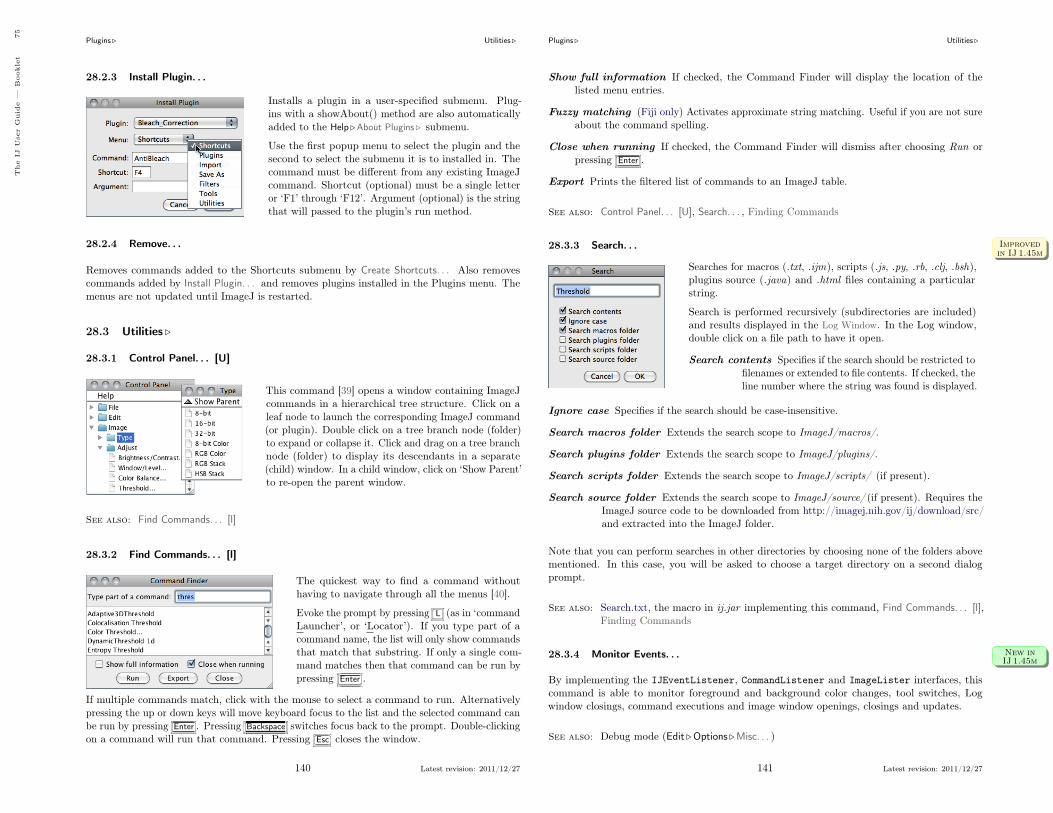
Plugins . Utilities .

28.2.3 Install Plugin. . .

Installs a plugin in a user-specified submenu. Plug-ins with a showAbout() method are also automaticallyadded to the Help .About Plugins . submenu.

Use the first popup menu to select the plugin and thesecond to select the submenu it is to installed in. Thecommand must be different from any existing ImageJcommand. Shortcut (optional) must be a single letteror ‘F1’ through ‘F12’. Argument (optional) is the stringthat will passed to the plugin’s run method.

28.2.4 Remove. . .

Removes commands added to the Shortcuts submenu by Create Shortcuts. . . Also removescommands added by Install Plugin. . . and removes plugins installed in the Plugins menu. Themenus are not updated until ImageJ is restarted.

28.3 Utilities .

28.3.1 Control Panel. . . [U]

This command [39] opens a window containing ImageJcommands in a hierarchical tree structure. Click on aleaf node to launch the corresponding ImageJ command(or plugin). Double click on a tree branch node (folder)to expand or collapse it. Click and drag on a tree branchnode (folder) to display its descendants in a separate(child) window. In a child window, click on ‘Show Parent’to re-open the parent window.

See also: Find Commands. . . [l]

28.3.2 Find Commands. . . [l]

The quickest way to find a command withouthaving to navigate through all the menus [40].

Evoke the prompt by pressing L (as in ‘commandLauncher’, or ‘Locator’). If you type part of acommand name, the list will only show commandsthat match that substring. If only a single com-mand matches then that command can be run bypressing Enter .

If multiple commands match, click with the mouse to select a command to run. Alternativelypressing the up or down keys will move keyboard focus to the list and the selected command canbe run by pressing Enter . Pressing Backspace switches focus back to the prompt. Double-clickingon a command will run that command. Pressing Esc closes the window.



Show full information If checked, the Command Finder will display the location of thelisted menu entries.

Fuzzy matching (Fiji only) Activates approximate string matching. Useful if you are not sureabout the command spelling.

Close when running If checked, the Command Finder will dismiss after choosing Run orpressing Enter .

Export Prints the filtered list of commands to an ImageJ table.

See also: Control Panel. . . [U], Search. . . , Finding Commands

28.3.3 Search. . . Improvedin IJ 1.45mImprovedin IJ 1.45m

Searches for macros (.txt, .ijm), scripts (.js, .py, .rb, .clj, .bsh),plugins source (.java) and .html files containing a particularstring.

Search is performed recursively (subdirectories are included)and results displayed in the Log Window. In the Log window,double click on a file path to have it open.

Search contents Specifies if the search should be restricted tofilenames or extended to file contents. If checked, theline number where the string was found is displayed.

Ignore case Specifies if the search should be case-insensitive.

Search macros folder Extends the search scope to ImageJ/macros/.

Search plugins folder Extends the search scope to ImageJ/plugins/.

Search scripts folder Extends the search scope to ImageJ/scripts/ (if present).

Search source folder Extends the search scope to ImageJ/source/ (if present). Requires theImageJ source code to be downloaded from http://imagej.nih.gov/ij/download/src/and extracted into the ImageJ folder.

Note that you can perform searches in other directories by choosing none of the folders abovementioned. In this case, you will be asked to choose a target directory on a second dialogprompt.

See also: Search.txt, the macro in ij.jar implementing this command, Find Commands. . . [l],Finding Commands

28.3.4 Monitor Events. . . New inIJ 1.45mNew inIJ 1.45m

By implementing the IJEventListener, CommandListener and ImageLister interfaces, thiscommand is able to monitor foreground and background color changes, tool switches, Logwindow closings, command executions and image window openings, closings and updates.

See also: Debug mode (Edit .Options .Misc. . . )


The

IJUser

Guid

e—

Bookle

t75


28.3.5 Monitor Memory. . .Improvedin IJ 1.45mImprovedin IJ 1.45m

Displays a continuously updated graph of ImageJ’s memoryutilization, which can be useful for detecting memory leaks.

Memory usage and running threads are displayed above thegraph. Clicking on the window will reclaim unused memoryby running the Java garbage collector (cf. Status bar).

Ideally you should be able to open several images, process them, close them, and the amount ofmemory used will be the same as when you started.

28.3.6 Capture Screen [g]

Copies the screen to an RGB image and displays that image a new window. Holding Ctrl ShiftG will capture the screen while a modal dialog box is active if the dialog is based on ImageJ’sGenericDialog class.

28.3.7 Capture Image

Copies a WYSIWYG version of active image to an RGB image and displays that image a newwindow.

See also: Flatten [F]

28.3.8 ImageJ Properties. . .

This command displays various ImageJ properties (Java version, OS name and version, pathseparator, location of directories, screen size, etc.) in a text window. Holding Alt lists all Javaproperties

See also: Status bar, Help .About ImageJ. . .

28.3.9 Threads. . .

This command lists, in a text window, the currently running threads and their priorities.

28.3.10 Benchmark

Runs 62 image processing operations on the current image and displays the elapsed time in theImageJ status bar. Additional benchmarks, test results, and source code are available in theBenchmarks package of plugins.

See also: FAQ’s on the ImageJ Documentation Wiki

28.3.11 Reset. . .

Use this command to unlock a locked Image, or to reclaimmemory used by the clipboard and undo buffers (cf. Undoand Redo).


Plugins . New .

28.4 New .

This submenu contains commands opening editor windows that can be used to edit and runmacros, scripts and plugins. It also has a command that opens a text window of a specified sizeand a command that opens a table that macros can write to. The editor windows opened byPlugin, Plugin Filter and Plugin Frame contain prototype Java code for the three types of pluginssupported by ImageJ.

See also: ImageJ Editor, Extending ImageJ

28.4.1 Macro

Opens a blank editor window with the title ‘Macro.txt’.

See also: Macros, ImageJ Editor, Text Window. . . , File .New .Text Window [N]

28.4.2 JavaScript

Opens a blank editor window with the title ‘Script.js’.

See also: Scripts, ImageJ Editor

28.4.3 Plugin

Opens an editor window containing a prototype plugin that implements the PlugIn interface.Plugins of this type open, capture or generate images. The prototype displays "Hello world!"in the ImageJ window. Press Ctrl R (File .Run Macro) to compile and run it. Note that thename you choose for the plugin should include at least one underscore. Another example is theStep Maker plugin.

28.4.4 Plugin Filter

Opens an editor window containing a prototype plugin that implements the PlugInFilterinterface. Plugins of this type process the active image. The prototype inverts the active imagetwice. Another example is the Image Inverter.

28.4.5 Plugin Frame

Opens an editor window containing a prototype plugin that extends the PlugInFrame class.Plugins of this type displays a window containing controls such as buttons and sliders. Theprototype opens a window containing a text area. Another example is the IP Demo plugin.


The

IJUser

Guid

e—

Bookle

t76

Plugins . Compile and Run. . .

28.4.6 Text Window. . .

Opens a text window of a specified size that macros can writeto. PrintToTextWindow, Clock and ProgressBar are examples ofmacros that write to a text window.

See also: Plugins .New .Macro, File .New .Text Window [N]

28.4.7 Table. . .

Opens a blank table, similar to the Results table, that macros canwrite to. SineCosineTable2 is an example of such a macro.

See also: Plugins .New .Text Window. . .

28.5 Compile and Run. . .

Compiles and runs a plugin. Runs a plugin if the name of the selected file ends in .class.Requires that ImageJ be running on a Java Virtual Machine that includes the javac compiler,which is contained in the Tools.jar archive. Tools.jar is included with the Windows and Linuxversions of ImageJ bundled with Java, and it is pre-installed on Mac OSX. Troubleshootinginformation can be found under ‘Compiling Plugins’ in the Linux and Windows release notes.

The Edit .Options .Compiler. . . command can be used to configure the javac compiler. SinceImageJ 1.44c and later, Compile and Run. . . adds the Bio-Formats plugin (loci_tools.jar) to theJava compiler’s classpath.


Window .

29 Window .

This menu contains four commands plus a list of open ImageJ windows. The currently activeimage will have a checkmark next to its name. To activate a window, pull down this menu andselect the window by name.

29.1 Show All [ ] ]

Makes all the windows associated with ImageJ visible.

29.2 Put Behind [tab]

Displays the next open image. Repeatedly press the tab key to cycle through all open images.Note that pressing Enter on any image will bring the ImageJ window to the foreground.

See also: I Frontmost Window and Windows Activation

29.3 Cascade

Moves all open images to the left side of the screen, slightly offset from each other, and displayedin the order they are listed at the bottom of this menu.

29.4 Tile

Shrinks all open image windows and repositions them to fit on the screen without overlapping.


The

IJUser

Guid

e—

Bookle

t77

Help .

30 Help .

Many of the commands in this menu use ImageJ’s BrowserLauncher to open a Web page usingthe user’s default browser. On Linux, BrowserLauncher looks for ‘netscape’, ‘firefox’, ‘konqueror’,‘mozilla’, ‘opera’, ‘epiphany’ or ‘lynx’ and uses the first one it finds.

30.1 ImageJ Website. . .

Opens the ImageJ home page.

30.2 ImageJ News. . .

Opens the News section of the ImageJ website.

30.3 Documentation. . .

Opens the Documentation section of the ImageJ website.

30.4 Installation. . .

Opens the Installation section of the ImageJ website specifically dedicated to the OS in whichImageJ is running, i.e either Linux, Mac OS 9, Mac OS X or Windows. Worth reading are thesections Known Problems and Troubleshooting.

30.5 Mailing List. . .Changedin IJ 1.45mChangedin IJ 1.45m

Opens the ImageJ Interest Group page on the NIH LISTSERV facility. Here you can search themailing list archives, post a message to the list, join or leave the list, or update options.

30.6 Dev. Resources. . .

Opens the Developer Resources section of the ImageJ website.

30.7 Plugins. . .

Opens the Plugins page on the ImageJ website, which lists more than 500 ImageJ plugins.

30.8 Macros. . .

Opens the macros directory on the ImageJ website, which contains more than 400 ImageJmacros.

30.9 Macro Functions. . .

Opens the Macro Functions reference page, an indispensable guide to the built in functions thatcan be called from the ImageJ macro language.

See also: Macros


Help . Update ImageJ. . .

30.10 Update ImageJ. . .

Upgrades ImageJ to the latest ij.jar at http://imagej.nih.gov/ij/upgrade/, or downgrades to one of the earlier versionsat http://imagej.nih.gov/ij/download/jars/. Select dailybuild from the drop-down menu and ImageJ will be upgradedto the latest daily build at http://imagej.nih.gov/ij/ij.jar.

See also: Installing and Maintaining ImageJ

30.11 Refresh Menus

Use this command to update ImageJ’s menus after adding (or removing) plugins or macros tothe plugins folder. Prior to ImageJ 1.44b this command was named ‘Update Menus’.

30.12 About Plugins .

This submenu displays information about some of the plugins in the ImageJ plugins folder. Tobe included in this submenu, a plugin must be packaged as a JAR file. There is an example atrsb.info.nih.gov/ij/plugins/jar-demo.html.

30.13 About ImageJ. . .

Opens an image containing informationabout the ImageJ version, the author, thewebsite, Java version and memory available.Note that clicking in the status bar is aquicker way to show this information.

See also: Plugins .Utilities . ImageJ Prop-erties. . . , Status bar


The

IJUser

Guid

e—

Bookle

t78

Part VI

Keyboard Shortcuts

The following table summarizes the keyboard shortcuts built into ImageJ. You can createadditional shortcuts, or override built-in ones, by creating simple macros and adding them tothe StartupMacros.txt. You can also assign a function key to a menu command using Plugins .Shortcuts .Create Shortcuts. . . .

Several of these shortcuts accept key modifiers as described in Key Modifiers. Also note that,except when using the text tool, you do not need to hold down the control key to use a keyboardshortcut (cf. Edit .Options .Misc. . . ).

See also: Using Keyboard Shortcuts, Finding Commands, Tools Shortcuts, KeyboardShort-cuts.txt macro, demonstrating how assign shortcuts to custom macros

List of ImageJ 1.45m built-in shortcuts. This table can be obtained within ImageJ using thePlugins . Shortcuts . List Shortcuts. . . command.

Command /Operation Shortcut Description

File .

New . Image. . . [n] N Create new image or stackNew .Text Window [N] Shift N Create new text windowNew . System Clipboard [V] Shift V Create image from system clipboardOpen. . . O Open file (any format recognized by ImageJ)Open Next [O] Shift O Open next image in folderOpen Samples .Blobs (25K) Shift B Opens the Blobs.gif example imageClose [w] W Close the active windowSave [s] S Save active image in Tiff formatRevert [r] R Revert to saved version of imagePrint. . . [p] P Print active image

Edit .

Undo [z] Z Undo last operationCut [x] X Copy selection to internal clipboard and clearCopy [c] C Copy selection to internal clipboardPaste [v] V Paste contents of internal clipboardClear Backspace Erase selection to background colorFill [f] F Fill selection in foreground colorDraw [d] D Draw selectionInvert [I] Shift I Invert image or selectionSelection .Select All [a] A Select entire imageSelection .Select None [A] Shift A Remove selectionSelection .Restore Selection [E] Shift E Restore previous selectionSelection .Properties. . . [y] Y Defines selection propertiesSelection .Add to Manager [t] T Add selection to ROI Manager

Image .

Adjust .Brightness/Contrast. . . [C] Shift C Adjust brightness and contrastAdjust .Threshold. . . [T] Shift T Adjust threshold levels

148

List of ImageJ 1.45m built-in shortcuts. This table can be obtained within ImageJ using thePlugins . Shortcuts . List Shortcuts. . . command.

Command /Operation Shortcut Description

Show Info. . . [i] I Display information about active imageProperties. . . [P] Shift P Display image propertiesColor .Color Picker. . . [K] Shift K Open Color PickerStacks .Next Slice [>] > or → Go to next stack sliceStacks .Previous Slice [<] < or ← Go to previous stack sliceStacks .Reslice. . . [/] / Reslice stackStacks .Orthogonal Views [H] Shift H Toggle orthogonal view displayStacks .Tools . Start Animation [\] \ Start/stop stack animationHyperstacks .Channels Tool. . . [Z] Shift Z Open the ‘Channels’ toolHyperstacks > or → Next hyperstack channelHyperstacks < or ← Previous hyperstack channelHyperstacks Ctrl > Next hyperstack sliceHyperstacks Ctrl < Previous hyperstack sliceHyperstacks Alt > Next hyperstack frameHyperstacks Alt < Previous hyperstack frameCrop [X] Shift X Crop active image or selectionDuplicate. . . [D] Shift D Duplicate active image or selectionScale. . . [E] E Scale image or selectionZoom . In [+] + or ↑ Make image largerZoom .Out [-] − or ↓ Make image smallerZoom .Original Scale [4] 4 Revert to original zoom levelZoom .View 100% [5] 5 Zoom to 1:1

Process .

Smooth [S] Shift S 3×3 unweighted smoothingRepeat Command [R] Shift R Repeat previous command

Analyze .

Measure. . . [m] M Display statistics of active image / selectionHistogram [h] H Display histogram of active image / selectionPlot Profile [k] K Display density profile plot of active selectionGels .Select First Lane 1 Select first gel laneGels .Select Next Lane 2 Select next gel lane

Plugins .

Utilities .Control Panel. . . [U] Shift U Open Control PanelUtilities .Capture Screen [g] Shift G Grab screenshotUtilities .Find Commands. . . [l] L List, find and launch commands

Window .

Show All [ ] ] ] Make all windows visiblePut Behind [tab] Tab Switch to next image windowImageJ window Enter Bring ImageJ window to front


The

IJUser

Guid

e—

Bookle

t79

Key Modifiers

31 Key Modifiers

31.1 Alt Key Modifications

File .Open Next Open previous

File .Revert Don’t show dialog

Edit .Copy Copy to system clipboard

Image .Color . Split Channels Keep original image

Image .Stacks .Add Slice Insert before current slice

Image .Stacks .Next Slice Skip nine slices

Image .Stacks .Previous Slice Skip nine slices

Image .Stacks . Start Animation Show options dialog

Image .Duplicate Don’t show dialog

Image .Overlay .Add Selection Don’t show dialog

Process .Equalize Do classic histogram equalization

Analyze .Histogram Show dialog

Analyze .Plot Profile For rectangular selections, generate row average plot

Analyze .Plot Profile For wide straight lines, display rotated contents

Analyze .Gels . Select First Lane Assume lanes are horizontal

Analyze .Tools .Analyze Line Graph Show intermediate image

Analyze .Tools .Roi Manager(Add) Name and add selection

Plugins .Utilities . ImageJ Properties List all Java properties

Any user plugin Load using new class loader

Area selection tools Subtract current selection from the previous one

Rectangle and Oval selection tools Current aspect ratio is maintained while resizing

Polygon selection tool Alt-click on a node to delete it

Straight line tool Keeps the line length fixed while moving either end of the line. Forces the twopoints that define the line to have integer coordinate values when creating a line on a zoomedimage

Segmented line tool Alt-click on a node to delete it

Point tool Alt-click on a point to delete it

Color picker tool Alt-click to ‘pick-up’ background color

All tools Show location and size in pixels

31.2 Shift Key Modifications

Image .Adjust .Threshold Adjusting Min also adjusts Max

Image .Adjust .Brightness/Contrast Apply adjustments to all channels of a composite image

Installed Macros and Scripts Open instead of run

Rectangle and Oval selection tools Forces 1:1 aspect ratio

Area selection tool Add this selection to previous one

Polygon selection tool Shift-click on a node to duplicate it

Straight line tool Forces line to be horizontal or vertical

Segmented line selection tool Shift-click on a node to duplicate it

Point selection tool Shift-click to add a point


Tools Shortcuts Ctrl Key (or Cmd) Modifications

31.3 Ctrl Key (or Cmd) Modifications

Rectangle and Oval selection tools (With Alt) Current aspect ratio is maintained while resizing

Rectangle and Oval selection tools Selection is resized around the center

Straight line tool Rotate/resize the line about its center

31.4 Space Bar

Any Tool Switch to the hand tool

31.5 Arrow Keys

Moving Selections The four arrow keys move selection outlines one pixel at a time

Resizing Selections Rectangular and oval selections are resized by holding Alt while using the arrowkeys

Stacks Navigation The ← and → keys substitute for < and > for moving through a stack. Ifthere is a selection, you must also hold Shift

Hyperstacks Navigation The ← and → keys change the channel. Hold Ctrl to move through theslices and Alt to move through the frames

Zooming The ↑ and ↓ keys zoom the image in and out. If there is a selection, you must also holdeither Shift or Ctrl

32 Tools Shortcuts

Keyboard shortcuts cannot be used directly to activate tools in the ImageJ toolbar (with theexception of the Magnifying Glass and the Scrolling Tool). However, shortcuts can be assignedto macros that use the setTool() function. Once copied to the to the ImageJ/macros/Startup-Macros.txt file ImageJ will automatically install them at start-up.

The set of macros listed below (taken from the Rename and Save ROI Sets toolset) exemplifythe use of the setTool() function by assigning the numeric keys 1–4 to the first four areaselection Area Selection Tools. The macro ‘Refine selection’ activates temporarily the brushselection tool when 5 is pressed. Once the mouse is released the previously selected tool isrestored.

(7) Assigning Keyboard Shortcuts to ImageJ Tools1 /* This set of macros exemplifies how to use the setTool () function to assign

hotkeys to ImageJ tools. */2

3 macro "Rectangle [1]" {setTool("rectangle");}4 macro "Ellipse [2]" {setTool("elliptical");}5 macro "Polygon [3]" {setTool("polygon");}6 macro "Freehand [4]" {setTool("freehand");}7 macro "Refine Area Selection [5]" {8 tool = IJ.getToolName;9 setTool("brush");

10 while (true) {11 getCursorLoc(x, y, z, flags);12 i f (flags&16!=0){setTool(tool); exit;}13 }14 }


The

IJUser

Guid

e—

Bookle

t80

Tools Shortcuts

This approach, however, requires the user to memorize as many shortcuts as the number of toolsin the toolbar. In addition, it may be difficult to assign so many hot-keys without conflictingwith previously defined ones (see List Shortcuts. . . ). Probably a more efficient way to control thetoolbar using the keyboard is to create macros that can cycle through all the tools in the ImageJtoolbar. The next example demonstrates such an approach. It is composed of two macrosactivated by F1 and F2 that iterate through the toolbar items from left to right (forward cycle)and right to left (reverse cycle).

(8) Cycling Through ImageJ Tools Using Keyboard Shortcuts1 /* These two macros loop through the tools listed in an array using "F1" and "

F2" as keyboard shortcuts (forward and reverse cycling). */2

3 var tIndx= 0;4 var tools= newArray("rectangle", "roundrect", "oval", "ellipse", "brush", "

polygon", "freehand", "line","freeline","polyline", "arrow", "wand", "dropper", "angle", "point","multipoint", "text");

5

6 macro "Cycle Tools Fwd [F1]"{7 setTool(tools[tIndx]);8 tIndx++;9 i f (tIndx==tools.length)

10 tIndx = 0;11 }12

13 macro "Cycle Tools Rwd [F2]" {14 tIndx--;15 i f (tIndx<0)16 tIndx = tools.length -1;17 setTool(tools[tIndx]);18 }


Credits

[C1] The ImageJ installer for Windows is created using the Inno Setup installer generator. ImageJ.exethe Windows that launches ImageJ (ij.jar) was contributed by George Silva.

[C2] Support for ZIP-compressed TIFFs was contributed by Jason Newton in IJ 1.45g.

[C3] The macro editor’s Function Finder (Macros .Find Functions...) was written by Jérôme Mutterer.

[C4] The Elliptical Selection Tool was contributed by Norbert Vischer.

[C5] The Brush Selection Tool is based on the ROI Brush Tool plugin from Tom Larkworthy andJohannes Schindelin.

[C6] Jean-Yves Tinevez and Johannes Schindelin (authors of the Fiji Arrow Tool) contributed code tothe Arrow Tool.

[C7] Michael Schmid, added 4–connected and 8–connected tracing with tolerance to the Wand Tool.

[C8] In IJ 1.43l and earlier, the File . Import .Results. . . command was based on Jérôme Mutterer’sImport_Results_Table macro.

[C9] Marcel van Herk added URLs support to the File . Import .Stack From List. . . command inIJ 1.45f.

[C10] Michael Schmid contributed improvements to the AVI reader and AVI writer plugins.

[C11] Karen Collins contributed improvements to the FITS_Writer (File . Save As .FITS. . . command).

[C12] The Edit .Selection .Fit Circle command, based on a MATLAB script by Nikolai Chernov, wascontributed by Michael Doube and Ved Sharma.

[C13] The Edit . Selection .Create Selection command is based on the Threshold_To_Selection pluginwritten by Johannes Schindelin.

[C14] The Color Picker (Image .Color .Color Picker. . . [K]) was written by Gali Baler, a 2003–2004intern from Bethesda-Chevy Chase High School.

[C15] The 16 different thresholding methods available in the Image .Adjust .Threshold. . . [T] tool wereimplemented by Gabriel Landini.

[C16] Michael Schmid contributed improvements to the downsizing kernel used by Image .Adjust .Size. . . and Image . Scale. . . [E] as well as undo support for Image . Scale. . . [E].

[C17] The Image .Adjust .Color Threshold. . . command implements Gabriel Landini’s Threshold Colourplugin.

[C18] The Reslice and the ZProject plugin (Image . Stacks .Reslice. . . [/] and Z Project. . . commands)were contributed by Patrick Kelly and Harvey Karten of the University of California, San Diego.

[C19] The Image . Stacks .Orthogonal Views [H] command is based on Dimiter Prodanov’s StackSlicerplugin and Albert Cardona’s Updater class. Michael Doube added support for XZ and YZ viewcontrol as well as mouse wheel control.

[C20] The Image .Stacks . 3D Project. . . was written by Michael Castle and Janice Keller of theUniversity of Michigan Mental Health Research Institute (MHRI). Bill Mohler added suport forhyperstacks and 16/32–bit images in IJ 1.44m.

[C21] The Image .Stacks .Tools .Make Substack. . . command is based on the Substack Maker pluginby Anthony Padua, Daniel Barboriak and Ved Sharma.

[C22] The Image .Hyperstacks .Reduce Dimensionality. . . command is based on Jérôme Mutterer’sReduce HyperStack macro.

[C23] The Image .Zoom . Set. . . command is based on Albert Cardona’s Zoom Exact plugin.

[C24] The Process .Find Maxima. . . command is based on a plugin contributed by Michael Schmid.

[C25] The equalization code implemented in Process .Enhance Contrast was contributed by RichardKirk.

153

The

IJUser

Guid

e—

Bookle

t81

[C26] The Process .Noise .Remove NaNs. . .was contributed by Michael Schmid.

[C27] The Process .Math .Macro. . . command is modeled after Ulf Dittmer’s Expression plugin.

[C28] The Process .FFT .Bandpass Filter. . . is a built in version of Joachim Walter’s FFT Filter plugin.

[C29] The Process .Binary .Fill Holes algorithm was contributed by Gabriel Landini.

[C30] Multi-threading support for all Process .Filters . commands was contributed by Stephan Saalfeldand Michael Schmid in ImageJ 1.45c.

[C31] The faster and more accurate version of Process .Filters .Gaussian Blur. . . implemented inImageJ 1.38r was contributed by Michael Schmid.

[C32] The NonBlockingGenericDialog.class used by the Process .Batch .Macro. . . command wasadded by Johannes Schindelin.

[C33] The Analyze .Distribution. . . command was written by Gabriel Landini.

[C34] The scaled color bar implemented in Analyze .Histogram [h] was contributed by Bob Dougherty.

[C35] The Rodboard and Gaussian functions implemented in (Analyze .Tools .Curve Fitting. . . ) werecontributed by David Rodbard (NIH) and Stefan Wörz (DKFZ), respectively.

[C36] The ROI Manager(XOR) command (Analyze .Tools .ROI Manager. . . ) was added by JohannesSchindelin.

[C37] The ROI Manager(Multi Measure) command (Analyze .Tools .ROI Manager. . . ) is based on BobDougherty’s Multi_Measure plugin.

[C38] The ROI Manager(Multi Plot) command (Analyze .Tools .ROI Manager. . . ) was contributed byPhilippe Gendre.

[C39] The Control Panel (Plugins .Utilities .Control Panel. . . [U]) was written by Cezar M. Tigare.

[C40] The Command Finder (Plugins .Utilities .Find Commands. . . [l]) was written by Mark Longair.

[C41] Other additions, improvements and bug fixes have been contributed by:Adrian Daerr, Albert Cardona, Alberto Duina, Alden Dima, Andreas Maier, Andrew French,Andrii Savchenko, Arttu Miettinen, Barry DeZonia, Bill Mohler, Bruno Vellutini, Carne Draug,Christian Moll, Daniel Kalthoff, Daniel Senff, David McDonald, Daniel Kalthoff, Dimiter Pro-danov, Divakar Ramachandran, Duncan Mak, Erik Meijering, Francis Burton, Frank Sprenger,Frederic Hessman, Gilles Carpentier, Gabriel Landini, Ingo Bartholomaeus, Jan Eglinger, JanFunke, Jarek Sacha, Jay Unruh, Jerome Mutterer, Joachim Wesner, Johannes Hermen, JohannesSchindelin, Johannes Weissmann, John Oreopoulos, John Pearl, Jonathan Silver, Juan Grande,Julian Cooper, Kai Uwe Barthel, Karen Collins, Kevin Moll, Kris Sheets, Mark Longair, MatAl-Tamimi, Matthew Smith, Michael Cammer, Michael Doube, Michael Ellis, Michael Schmid,Nico Stuurman, Norbert Vischer, Olaf Freyer, Peter Haub, Reinhard Mayr, Richard Cole, RobertDougherty, Shannon Stewman, Simon Roussel, Stefan Starke, Stephan Saalfeld, Tiago Ferreira,Tomas Karlsson, Tseng Qingzong, Ulf Dittmer, Uwe Walschus, Valerio Mussi, Ved Sharma, VytasBindokas, Wilhelm Burger.

[C42] Macro Toolsets distributed with ImageJ have been contributed by:Gilles Carpentier (Arrow Labelling Tools.txt, Scale Bar Tools for Microscopes.txt), JérômeMutterer (Example Icons.txt, Magic Montage.txt), Tiago Ferreira (Toolset Creator.txt).

154

ImageJ Related Publications

The following references are a small sample of the bibliography directly related to ImageJ, the standardin scientific image analysis. These publications include: 1) technical articles and books describing routinesimplemented in ImageJ, 2) research articles that have made extensive use of ImageJ as a scientifictool or 3) reviews that discuss ImageJ pertinently. This list appears in chronological order rather thanalphabetical and is particularly biased towards the life sciences.

To reference ImageJ one of the following citations is possible:

1. Rasband, W.S., ImageJ, U.S. National Institutes of Health, Bethesda, Maryland, USA, imagej.nih.gov/ij/, 1997–2011.

2. Abràmoff, M.D., Magalhães, P.J. and Ram, S.J. Image Processing with ImageJ. BiophotonicsInternational, 11(7):36–42, 2004 (PDF) [102].

To reference this document:

– Ferreira T. and Rasband W. (2010-2011) The mageJ User Guide — IJ 1.45, imagej.nih.gov/ij/docs/guide/.

[1] Janos Kriston-Vizi, Ng Wee Thong, Cheok Leong Poh, Kwo Chia Yee, Joan Sim Poh Ling, RachelKraut, and Martin Wasser. Gebiss: an imagej plugin for the specification of ground truth and theperformance evaluation of 3d segmentation algorithms. BMC Bioinformatics, 12:232, 2011.

[2] Michael Doube, Michal M Klosowski, Ignacio Arganda-Carreras, Fabrice P Cordelieres, Robert PDougherty, Jonathan S Jackson, Benjamin Schmid, John R Hutchinson, and Sandra J Shefelbine.BoneJ: Free and extensible bone image analysis in ImageJ. Bone, 47(6):1076–9, Dec 2010.

[3] Simon Andrews, Jonathan Gilley, and Michael P Coleman. Difference Tracker: ImageJ plugins forfully automated analysis of multiple axonal transport parameters. J Neurosci Methods, 193(2):281–7,Nov 2010.

[4] Arthur Edelstein, Nenad Amodaj, Karl Hoover, Ron Vale, and Nico Stuurman. Computer controlof microscopes using µManager. Curr Protoc Mol Biol, Chapter 14:Unit14.20, Oct 2010.

[5] Michael J M Fischer, Sae Uchida, and Karl Messlinger. Measurement of meningeal blood vesseldiameter in vivo with a plug-in for ImageJ. Microvasc Res, 80(2):258–66, Sep 2010.

[6] Ricardo Henriques, Mickael Lelek, Eugenio F Fornasiero, Flavia Valtorta, Christophe Zimmer,and Musa M Mhlanga. QuickPALM: 3D real-time photoactivation nanoscopy image processing inImageJ. Nat Methods, 7(5):339–40, May 2010.

[7] Thomas Walter, David W Shattuck, Richard Baldock, Mark E Bastin, Anne E Carpenter, SuzanneDuce, Jan Ellenberg, Adam Fraser, Nicholas Hamilton, Steve Pieper, Mark A Ragan, Jurgen ESchneider, Pavel Tomancak, and Jean-Karim Hériché. Visualization of image data from cells toorganisms. Nature Methods, 7(3 Suppl):S26–41, Mar 2010.

[8] Sascha Meyer Dos Santos, Ute Klinkhardt, Reinhard Schneppenheim, and Sebastian Harder. UsingImageJ for the quantitative analysis of flow-based adhesion assays in real-time under physiologicflow conditions. Platelets, 21(1):60–6, Feb 2010.

[9] Albert Cardona, Stephan Saalfeld, Stephan Preibisch, Benjamin Schmid, Anchi Cheng, Jim Pulokas,Pavel Tomancak, and Volker Hartenstein. An integrated micro- and macroarchitectural analysis ofthe Drosophila brain by computer-assisted serial section electron microscopy. PLoS Biol, 8(10),Jan 2010.

[10] Adam S Green, Paul R Ohmann, Nick E Leininger, and James A Kavanaugh. Polarization Imagingand Insect Vision. The Physics Teacher, 48:17, Jan 2010. (c) 2010: American Institute of Physics.

[11] E Iannuccelli, F Mompart, J Gellin, Y Lahbib-Mansais, M Yerle, and T Boudier. NEMO: a tool foranalyzing gene and chromosome territory distributions from 3D-FISH experiments. Bioinformatics(Oxford, England), Jan 2010.

155

The

IJUser

Guid

e—

Bookle

t82

[12] Christof Karmonik, Michele York, Robert Grossman, Ekta Kakkar, Krutina Patel, Hani Haykal,and David King. An image analysis pipeline for the semi-automated analysis of clinical fMRIimages based on freely available software. Computers in biology and medicine, Jan 2010.

[13] Benjamin Schmid, Johannes Schindelin, Albert Cardona, Mark Longair, and Martin Heisenberg. Ahigh-level 3D visualization API for Java and ImageJ. BMC Bioinformatics 2010 11:274, 11:274,Jan 2010.

[14] German Kilimnik, Abraham Kim, Junghyo Jo, Kevin Miller, and Manami Hara. Quantification ofpancreatic islet distribution in situ in mice. Am J Physiol Endocrinol Metab, 297(6):E1331–8, Dec2009.

[15] Atsuko Kobayashi, Takumi Fujigaya, Masayuki Itoh, Takahisa Taguchi, and Hiroshi Takano.Technical note: a tool for determining rotational tilt axis with or without fiducial markers.Ultramicroscopy, 110(1):1–6, Dec 2009.

[16] Philippe Mailly, Suzanne N Haber, Henk J Groenewegen, and Jean-Michel Deniau. A 3D multi-modal and multi-dimensional digital brain model as a framework for data sharing. J NeurosciMethods, Dec 2009.

[17] Richard L Mort. Quantitative analysis of patch patterns in mosaic tissues with ClonalTools software.J Anat, 215(6):698–704, Dec 2009.

[18] T Vrekoussis, V Chaniotis, I Navrozoglou, V Dousias, K Pavlakis, E N Stathopoulos, and O Zoras.Image analysis of breast cancer immunohistochemistry-stained sections using ImageJ: an RGB-basedmodel. Anticancer Res, 29(12):4995–8, Dec 2009.

[19] Emel Bulut and Bünyamin Sahin. A new method of assessing the size of mandibular cysts onorthopantomograms: projection area fraction. J Craniofac Surg, 20(6):2020–3, Nov 2009.

[20] J Hegyi, V Hegyi, G Messer, P Arenberger, T Ruzicka, and C Berking. Confocal laser-scanningcapillaroscopy: a novel approach to the analysis of skin capillaries in vivo. Skin Res Technol,15(4):476–81, Nov 2009.

[21] Jason R Swedlow and Kevin W Eliceiri. Open source bioimage informatics for cell biology. Trendsin Cell Biology, 19(11):656–60, Nov 2009.

[22] Clayton M Costa and Suann Yang. Counting pollen grains using readily available, free imageprocessing and analysis software. Ann Bot, 104(5):1005–10, Oct 2009.

[23] Nicola Goodall, Lilian Kisiswa, Ankush Prashar, Stuart Faulkner, Paweł Tokarczuk, Krish Singh,Jonathan T Erichsen, Jez Guggenheim, Willi Halfter, and Michael A Wride. 3-Dimensionalmodelling of chick embryo eye development and growth using high resolution magnetic resonanceimaging. Exp Eye Res, 89(4):511–21, Oct 2009.

[24] Fathima Shihana, Dhammika Menike Dissanayake, Nicholas Allan Buckley, and Andrew HamiltonDawson. A Simple Quantitative Bedside Test to Determine Methemoglobin. Ann Emerg Med, Oct2009.

[25] János Roszik, Duarte Lisboa, János Szöllosi, and György Vereb. Evaluation of intensity-basedratiometric FRET in image cytometry–approaches and a software solution. Cytometry A, 75(9):761–7, Sep 2009.

[26] Edmund Y Tong, Geoffrey C Collins, April E Greene-Colozzi, Julia L Chen, Philip D Manos,Kyle M Judkins, Joseph A Lee, Michael J Ophir, Farrah M Laliberte, and Timothy J Levesque.Motion-based angiogenesis analysis: a simple method to quantify blood vessel growth. Zebrafish,6(3):239–43, Sep 2009.

[27] Stephan Saalfeld, Albert Cardona, Volker Hartenstein, and Pavel Tomancák. CATMAID: collabo-rative annotation toolkit for massive amounts of image data. Bioinformatics (Oxford, England),25(15):1984–6, Aug 2009.

[28] David J Barry, Cecilia Chan, and Gwilym A Williams. Morphological quantification of filamentousfungal development using membrane immobilization and automatic image analysis. J Ind MicrobiolBiotechnol, 36(6):787–800, Jun 2009.

156

[29] Stephan Hegge, Mikhail Kudryashev, Ashley Smith, and Friedrich Frischknecht. Automatedclassification of Plasmodium sporozoite movement patterns reveals a shift towards productivemotility during salivary gland infection. Biotechnol J, 4(6):903–13, Jun 2009.

[30] G Landini and G Perryer. Digital enhancement of haematoxylin- and eosin-stained histologicalimages for red-green colour-blind observers. J Microsc, 234(3):293–301, Jun 2009.

[31] Richard M Lindley, Daniel B Hawcutt, M Gwen Connell, David H Edgar, and Simon E Kenny.Properties of secondary and tertiary human enteric nervous system neurospheres. J Pediatr Surg,44(6):1249–55; discussion 1255–6, Jun 2009.

[32] Stephan Preibisch, Stephan Saalfeld, and Pavel Tomancak. Globally optimal stitching of tiled 3Dmicroscopic image acquisitions. Bioinformatics (Oxford, England), 25(11):1463–5, Jun 2009.

[33] Delphine S A Beeckman, Geert Meesen, Patrick Van Oostveldt, and Daisy Vanrompay. Digitaltitration: automated image acquisition and analysis of load and growth of Chlamydophila psittaci.Microsc. Res. Tech., 72(5):398–402, May 2009.

[34] A J Hand, T Sun, D C Barber, D R Hose, and S MacNeil. Automated tracking of migrating cellsin phase-contrast video microscopy sequences using image registration. Journal of microscopy,234(1):62–79, Apr 2009.

[35] Tal Shprung and Illana Gozes. A novel method for analyzing mitochondrial movement: inhibitionby paclitaxel in a pheochromocytoma cell model. J Mol Neurosci, 37(3):254–62, Mar 2009.

[36] Evan C Crawford and James K Mortensen. An ImageJ plugin for the rapid morphologicalcharacterization of separated particles and an initial application to placer gold analysis. Computers& Geosciences, 35:347, Feb 2009.

[37] Manuel G Forero, Jenny A Pennack, Anabel R Learte, and Alicia Hidalgo. DeadEasy Caspase:Automatic Counting of Apoptotic Cells in Drosophila. Plos One, 4(5):e5441, Jan 2009.

[38] C Igathinathane, LO Pordesimo, and WD Batchelor. Major orthogonal dimensions measurementof food grains by machine vision using ImageJ. Food Res Int, 42(1):76–84, Jan 2009.

[39] Noel Jabbour, Priya D Krishna, James Osborne, and Clark A Rosen. A new approach to geometricalmeasurements in an animal model of vocal fold scar. J Voice, 23(1):88–94, Jan 2009.

[40] Yoonseok Kam, Audrey Karperien, Brandy Weidow, Lourdes Estrada, Alexander R Anderson,and Vito Quaranta. Nest expansion assay: a cancer systems biology approach to in vitro invasionmeasurements. BMC Res Notes, 2:130, Jan 2009.

[41] H M Macdonald, D M L Cooper, and H A McKay. Anterior-posterior bending strength at thetibial shaft increases with physical activity in boys: evidence for non-uniform geometric adaptation.Osteoporos Int, 20(1):61–70, Jan 2009.

[42] Peter A McAtee, Ian C Hallett, Jason W Johnston, and Robert J Schaffer. A rapid method offruit cell isolation for cell size and shape measurements. Plant Methods, 5:5, Jan 2009.

[43] Ricardo B Medeiros, Kate J Papenfuss, Brian Hoium, Kristen Coley, Joy Jadrich, Saik-Kia Goh,Anuratha Elayaperumal, Julio E Herrera, Ernesto Resnik, and Hsiao-Tzu Ni. Novel sequentialChIP and simplified basic ChIP protocols for promoter co-occupancy and target gene identificationin human embryonic stem cells. BMC Biotechnol, 9:59, Jan 2009.

[44] Christopher A Myrick. A low-cost system for capturing and analyzing the motion of aquaticorganisms. J N Am Benthol Soc, 28(1):101–109, Jan 2009.

[45] Jonathan Popko, Adelaide Fernandes, Dora Brites, and Lorene M Lanier. Automated Analysis ofNeuronJ Tracing Data. Cytom Part A, 75A(4):371–376, Jan 2009.

[46] Zhuang Tian, Li Qiang Liu, Chifang Peng, Zhenxing Chen, and Chuanlai Xu. A new developmentof measurement of 19-Nortestosterone by combining immunochromatographic strip assay andImageJ software. Food Agr Immunol, 20(1):1–10, Jan 2009.

[47] Jun Xu and Dong Chen. Desing and Implementation of the Image Format Batch-ConversionSoftware Based on ImageJ. Astronomical Research and Technology. Publications of NationalAstronomical Observatories of China (ISSN 1672-7673), 5:270, Sep 2008.

157

The

IJUser

Guid

e—

Bookle

t83

[48] David Hecker, Joachim Kappler, Alexander Glassmann, Karl Schilling, and Wolfgang Alt. Imageanalysis of time-lapse movies–a precision control guided approach to correct motion artefacts. JNeurosci Methods, 172(1):67–73, Jul 2008.

[49] Dilraj Grewal, Rajeev Jain, Gagandeep Singh Brar, and Satinder Pal Singh Grewal. Pentacamtomograms: a novel method for quantification of posterior capsule opacification. Invest OphthalmolVis Sci, 49(5):2004–8, May 2008.

[50] Madeline Pool, Joachim Thiemann, Amit Bar-Or, and Alyson E Fournier. NeuriteTracer: a novelImageJ plugin for automated quantification of neurite outgrowth. J Neurosci Methods, 168(1):134–9,Feb 2008.

[51] Wilhelm Burger and Mark James Burge. Digital image processing: An algorithmic introductionusing Java. ISBN 978-1-84628-379-6, Springer, Jan 2008.

[52] C Igathinathane, LO Pordesimo, EP Columbus, WD Batchelor, and SR Methuku. Shape identifi-cation and particles size distribution from basic shape parameters using ImageJ. Comput ElectronAgr, 63(2):168–182, Jan 2008.

[53] Anna Kirilova, Gina Lockwood, M Math, Perry Choi, Neelufer Bana, Masoom A Haider, Kristy KBrock, Cynthia Eccles, and Laura A Dawson. Three-dimensional motion of liver tumors usingcine-magnetic resonance imaging. Int J Radiat Oncol, 71(4):1189–1195, Jan 2008.

[54] Mahdad Noursadeghi, Jhen Tsang, Thomas Haustein, Robert F Miller, Benjamin M Chain, andDavid R Katz. Quantitative imaging assay for NF-κB nuclear translocation in primary humanmacrophages. J Immunol Methods, 329(1-2):194–200, Jan 2008.

[55] János Roszik, János Szöllosi, and György Vereb. AccPbFRET: an ImageJ plugin for semi-automatic,fully corrected analysis of acceptor photobleaching FRET images. BMC Bioinformatics, 9:346, Jan2008.

[56] Ruggero Scorcioni, Susan N Wright, JPatrick Card, Giorgio A Ascoli, and German Barrionuevo.Point analysis in Java applied to histological images of the perforant pathway: A user’s account,Jan 2008.

[57] S Sieuwerts, FAM de Bok, E Mols, WM de Vos, and JETvan Hylckama Vlieg. A simple and fastmethod for determining colony forming units. Lett Appl Microbiol, 47(4):275–278, Jan 2008.

[58] Simon A W G Dello, Ronald M van Dam, Jules J G Slangen, Marcel C G van de Poll, MarcH A Bemelmans, Jan Willem W M Greve, Regina G H Beets-Tan, Stephen J Wigmore, andCornelis H C Dejong. Liver volumetry plug and play: do it yourself with ImageJ. World J Surg,31(11):2215–21, Nov 2007.

[59] Stéphane Kerner, Daniel Etienne, Jacques Malet, Francis Mora, Virginie Monnet-Corti, andPhilippe Bouchard. Root coverage assessment: validity and reproducibility of an image analysissystem. J Clin Periodontol, 34(11):969–76, Nov 2007.

[60] Gary Chinga, Per Olav Johnsen, Robert Dougherty, Elisabeth Lunden Berli, and Joachim Walter.Quantification of the 3D microstructure of SC surfaces. Journal of microscopy, 227(Pt 3):254–65,Sep 2007.

[61] Eckard Picht, Aleksey V Zima, Lothar A Blatter, and Donald M Bers. SparkMaster: automatedcalcium spark analysis with ImageJ. Am J Physiol, Cell Physiol, 293(3):C1073–81, Sep 2007.

[62] A Solé, J Mas, and I Esteve. A new method based on image analysis for determining cyanobacterialbiomass by CLSM in stratified benthic sediments. Ultramicroscopy, 107(8):669–73, Aug 2007.

[63] David Stepensky. FRETcalc plugin for calculation of FRET in non-continuous intracellularcompartments. Biochem. Biophys. Res. Commun., 359(3):752–8, Aug 2007.

[64] Tony J Collins. ImageJ for microscopy. BioTechniques, 43(1 Suppl):25–30, Jul 2007.

[65] Martha L Narro, Fan Yang, Robert Kraft, Carola Wenk, Alon Efrat, and Linda L Restifo.NeuronMetrics: software for semi-automated processing of cultured neuron images. Brain Res.,1138:57–75, Mar 2007.

158

[66] Kevin M Schartz, Kevin S Berbaum, Robert T Caldwell, and Mark T Madsen. WorkstationJ:workstation emulation software for medical image perception and technology evaluation research.Medical Imaging 2007: Image Perception, 6515:49, Mar 2007.

[67] Brian A Irving, Judy Y Weltman, David W Brock, Christopher K Davis, Glenn A Gaesser, andArthur Weltman. NIH ImageJ and Slice-O-Matic computed tomography imaging software toquantify soft tissue. Obesity (Silver Spring), 15(2):370–6, Feb 2007.

[68] Philippe Thévenaz and Michael Unser. User-friendly semiautomated assembly of accurate imagemosaics in microscopy. Microsc. Res. Tech., 70(2):135–46, Feb 2007.

[69] Jonas G Wilson-Leedy and Rolf L Ingermann. Development of a novel CASA system based onopen source software for characterization of zebrafish sperm motility parameters. Theriogenology,67(3):661–72, Feb 2007.

[70] R Carmona, D Macías, J A Guadix, V Portillo, J M Pérez-Pomares, and R Muñoz-Chápuli. Asimple technique of image analysis for specific nuclear immunolocalization of proteins. Journal ofmicroscopy, 225(Pt 1):96–9, Jan 2007.

[71] R Cathelin, F Lopez, and Ch Klopp. AGScan: a pluggable microarray image quantification softwarebased on the ImageJ library. Bioinformatics, 23(2):247–248, Jan 2007.

[72] B Choi, C Nelson, Y Tsunashima, and P Balter. Open source, ImageJ based, web accessible toolfor treatment plan evaluation. Med Phys, 34(6):2477–2477, Jan 2007.

[73] L Ferrer, T Carlier, A Lisbona, and M Bardies. An imageJ plugin to create whole body transmissionscan using CT scanner: a validation study. Eur J Nucl Med Mol I, 34:S198–S198, Jan 2007.

[74] Charles A Lessman, Ravikanth Nathani, Rafique Uddin, Jamie Walker, and Jianxiong Liu.Computer-aided meiotic maturation assay (CAMMA) of zebrafish (Danio rerio) oocytes in vitro.Mol Reprod Dev, 74(1):97–107, Jan 2007.

[75] Cédric Messaoudii, Thomas Boudier, Carlos Oscar Sanchez Sorzano, and Sergio Marco. TomoJ:tomography software for three-dimensional reconstruction in transmission electron microscopy.BMC Bioinformatics, 8:288, Jan 2007.

[76] Francesca Papadopulos, Matthew Spinelli, Sabrina Valente, Laura Foroni, Catia Orrico, FrancescoAlviano, and Gianandrea Pasquinelli. Common tasks in microscopic and ultrastructural imageanalysis using ImageJ. Ultrastruct Pathol, 31(6):401–7, Jan 2007.

[77] Joel B Sheffield. ImageJ, a useful tool for biological image processing and analysis. MicroscMicroanal, 13:200–201, Jan 2007.

[78] Anne E Carpenter, Thouis R Jones, Michael R Lamprecht, Colin Clarke, In Han Kang, Ola Friman,David A Guertin, Joo Han Chang, Robert A Lindquist, Jason Moffat, Polina Golland, and David MSabatini. Cellprofiler: image analysis software for identifying and quantifying cell phenotypes.Genome Biol, 7(10):R100, Dec 2006.

[79] Muriel Hachet-Haas, Noël Converset, Olivier Marchal, Hans Matthes, Sophie Gioria, Jean-LucGalzi, and Sandra Lecat. FRET and colocalization analyzer–a method to validate measurementsof sensitized emission FRET acquired by confocal microscopy and available as an ImageJ Plug-in.Microsc. Res. Tech., 69(12):941–56, Dec 2006.

[80] R Ropolo, O Rampado, P Isoardi, A Izzo, L Savio, T Cammarota, O Davini, R De Lucchi, andG Gandini. Automated quality control in computed radiography. Radiol Med, 111(8):1156–67, Dec2006.

[81] S Bolte and F P Cordelières. A guided tour into subcellular colocalization analysis in lightmicroscopy. Journal of microscopy, 224(Pt 3):213–32, Nov 2006.

[82] J C Grochowsky, L W Alaways, R Siskey, E Most, and S M Kurtz. Digital photogrammetryfor quantitative wear analysis of retrieved TKA components. J Biomed Mater Res Part B ApplBiomater, 79(2):263–7, Nov 2006.

[83] Cédric Messaoudi, Nicole Garreau de Loubresse, Thomas Boudier, Pascale Dupuis-Williams, andSergio Marco. Multiple-axis tomography: applications to basal bodies from Paramecium tetraurelia.Biol Cell, 98(7):415–25, Jul 2006.

159

The

IJUser

Guid

e—

Bookle

t84

[84] John D Gottsch, Olof H Sundin, Erik V Rencs, David G Emmert, Walter J Stark, Clement JCheng, and Gregory W Schmidt. Analysis and documentation of progression of Fuchs cornealdystrophy with retroillumination photography. Cornea, 25(4):485–9, May 2006.

[85] Seth T Gammon, W Matthew Leevy, Shimon Gross, George W Gokel, and David Piwnica-Worms.Spectral unmixing of multicolored bioluminescence emitted from heterogeneous biological sources.Anal Chem, 78(5):1520–7, Mar 2006.

[86] XMa and MSHutson. Quantifying the intercellular forces during drosophila morphogenesis. Ameri-can Physical Society, page 29003, Mar 2006.

[87] W Bailer. Writing ImageJ Plugins–A Tutorial. Upper Austria University of Applied SciencesDept. of Media Technology and Design Hagenberg, Austria, http://www.gm.fh-koeln.de/~konen/WPF-BV/ tutorial-ImageJ_V1.71.pdf , Jan 2006.

[88] M Doube. ImageJ and analysis of correlated confocal and BSE-SEM imaging. Scanning, 28(2):93–94,Jan 2006.

[89] Y J Kim, B F M Romeike, J Uszkoreit, and W Feiden. Automated nuclear segmentation in thedetermination of the Ki-67 labeling index in meningiomas. Clin Neuropathol, 25(2):67–73, Jan2006.

[90] Jennifer L West and Ian D Cameron. Using the medical image processing package, ImageJ, forastronomy. arXiv, astro-ph, Jan 2006.

[91] A M Bell, K Parton, and E Smith. EarthTutor: An Interactive Intelligent Tutoring System forRemote Sensing. American Geophysical Union, 52:08, Dec 2005. (c) 2005: American GeophysicalUnion.

[92] Jérôme N Feige, Daniel Sage, Walter Wahli, Béatrice Desvergne, and Laurent Gelman. PixFRET, anImageJ plug-in for FRET calculation that can accommodate variations in spectral bleed-throughs.Microsc. Res. Tech., 68(1):51–8, Sep 2005.

[93] Daniel Sage, Franck R Neumann, Florence Hediger, Susan M Gasser, and Michael Unser. Automatictracking of individual fluorescence particles: application to the study of chromosome dynamics.IEEE Trans Image Process, 14(9):1372–83, Sep 2005.

[94] Daniel P Barboriak, Anthony O Padua, Gerald E York, and James R Macfall. Creation ofDICOM–aware applications using ImageJ. J Digit Imaging, 18(2):91–9, Jun 2005.

[95] Thomas Carlier, Ludovic Ferrer, Jean B Berruchon, Regis Cuissard, Adeline Martineau, PierreLoonis, and Olivier Couturier. Quality controls for gamma cameras and PET cameras: developmentof a free open-source ImageJ program. Medical Imaging 2005: Physics of Medical Imaging. Editedby Flynn, 5745:1237, Apr 2005.

[96] Derick Lau, Anthony Seibert, David Gandara, Luko Laptalo, Este Geraghty, and ChristopherCoulon. Computer-assisted image analysis of bronchioloalveolar carcinoma. Clin Lung Cancer,6(5):281–6, Mar 2005.

[97] Kerry M Brown, Duncan E Donohue, Giampaolo D’Alessandro, and Giorgio A Ascoli. A cross-platform freeware tool for digital reconstruction of neuronal arborizations from image stacks.Neuroinformatics, 3(4):343–60, Jan 2005.

[98] Eben Gering and Carter T Atkinson. A rapid method for counting nucleated erythrocytes onstained blood smears by digital image analysis. J Parasitol, 90(4):879–81, Aug 2004.

[99] E Meijering, M Jacob, J-C F Sarria, P Steiner, H Hirling, and M Unser. Design and validation ofa tool for neurite tracing and analysis in fluorescence microscopy images. Cytometry. Part A : thejournal of the International Society for Analytical Cytology, 58(2):167–76, Apr 2004.

[100] L Ferrer, Y Grealou, D Autret, S Gaudaire, G Brunet, G Delpon, A Lisbona, B Bridji, I Resche,C Rousseau, T Carlier, and M BardiAs. A new ImageJ plugin to correct for partial effect volume.Eur J Nucl Med Mol I, 31:S230–S230, Jan 2004.

[101] K Moodley and H Murrell. A colour-map plugin for the open source, Java based, image processingpackage, ImageJ. Computers & Geosciences, 30(6):609–618, Jan 2004.

160

[102] MD Abramoff, PJ Magalhaes, and S J Ram. Image Processing with ImageJ. BiophotonicsInternational (available at http://webeye.ophth.uiowa.edu/dept/biograph/abramoff/imagej.pdf),11(7):36–42, 2004.

[103] F. Leymarie and M. D. Levine. Fast raster scan distance propagation on the discrete rectangularlattice. CVGIP: Image Understanding, 55(1):84–94, 1992.

161

The

IJUser

Guid

e—

Bookle

t85

List of Abbreviations and Acronyms

Alt . . . . . . . . . . . Alt, Option or Meta key;

API . . . . . . . . . . . Application ProgrammingInterface;

ASCII . . . . . . . . American Standard Code forInformation Interchange;

bit . . . . . . . . . . . . Binary digit;

BMP . . . . . . . . . Bitmap Image File (DeviceIndependent Bitmap, DIB);

bpp . . . . . . . . . . . Bits per pixel;

CCD . . . . . . . . . . Charge-Coupled Device;

CP . . . . . . . . . . . Color Picker;

CSV . . . . . . . . . . Comma-Separated Values;

CT . . . . . . . . . . . Computed Tomography;

Ctrl . . . . . . . . . . . Control key. In this guide also theCommand key in Applekeyboards;

DICOM . . . . . . . Digital Imaging andCommunications in Medicine;

DPI . . . . . . . . . . . Dots Per Inch;

EDM . . . . . . . . . Euclidian Distance Map;

FAQ . . . . . . . . . . Frequently Asked Questions;

FFT . . . . . . . . . . Fast Fourier Transform;

FHT . . . . . . . . . . Fast Hartley Transform;

FIJI . . . . . . . . . . Fiji Is Just ImageJ;

FITS . . . . . . . . . Flexible Image Transport System;

fps . . . . . . . . . . . . Frames Per Second;

GIF . . . . . . . . . . . Graphics Interchange Format;

GUI . . . . . . . . . . Graphical User Interface;

HDR . . . . . . . . . . High Dynamic Range;

HEX . . . . . . . . . . Hexadecimal;

HIPR . . . . . . . . . Hypermedia Image ProcessingReference;

HSB . . . . . . . . . . Hue Saturation Brightness;

HTML . . . . . . . . HyperText Markup Language;

IJ . . . . . . . . . . . . . ImageJ;

JAR . . . . . . . . . . Java ARchive;

JPEG . . . . . . . . . Joint Photographic ExpertsGroup;

LUT . . . . . . . . . . Lookup table;

LZW . . . . . . . . . . Lempel-Ziv-Welch;

MIP . . . . . . . . . . Maximum Intensity Projection;

MJPG . . . . . . . . Motion-JPEG;

NaN . . . . . . . . . . Not a Number;

OS . . . . . . . . . . . . Operating System;

p/c . . . . . . . . . . . Pixels per cycle;

PBM . . . . . . . . . Portable BitMap;

PGM . . . . . . . . . Portable GrayMap;

pixel . . . . . . . . . . Picture element;

PNG . . . . . . . . . . Portable Network Graphics;

ppi . . . . . . . . . . . . Pixels per inch;

PPM . . . . . . . . . Portable PixMap;

RAM . . . . . . . . . Random-Access Memory;

regex . . . . . . . . . Regular expression;

RGB . . . . . . . . . . Red Green Blue;

ROI . . . . . . . . . . Region Of Interest;

Shift . . . . . . . . . . Shift key;

TIFF . . . . . . . . . Tagged Image File Format;

UEPs . . . . . . . . . Ultimate Eroded Points;

URL . . . . . . . . . . Uniform Resource Locator;

voxel . . . . . . . . . . Volumetric pixel;

WYSIWYG . . . What You See Is What You Get;

162

Index

AAcceptable manipulation, 5ActionBar, 22Add see Math, 102Add images see Image

calculator, 113Alpha blending value see

Blend, 92Analyze, 117AND see Logical operations,

114, 135Angle tool, 30Animation, 47, 84Annotations, 29, 31, 74

Grayscale images, 75Appearance, 59, 88Area, 122Area under the curve see

Definite integral, 129Arrows, 29Aspect ratio, 26, 27, 70, 123AutoRun, 19, 41AVI, 11, 46, 49

BBackground see Subtract

Background, 114Background pixels, 131Batch processing, 111, 138BeanShell, 22Benchmark, 142Bicubic interpolation see

Interpolation, 70Bilinear interpolation see

Interpolation, 70Binary, 98, 99Bio7, 4Bio-formats see LOCI, 11Bitwise operations, 103, 104Black background, 68, 99,

102Blend, 89, 92Bounding box, 53, 56Brightness/Contrast, 65–67,

95Brush selection tool, 27Bug (reporting) see also

Debug, 7

CCalibration, 126

Optical density, 125, 137Spatial, 72, 124, 136

Calibration bar, 137Caliper length see Feret, 123

Canvas, 71Capture image, 142Catmull-Rom see

Interpolation, 70CCD, 14, 97Cell Counter plugin, 30, 31CellProfiler see

Interoperability, 24Center of mass, 122Centroid, 122Channels, 72, 85CIE, 70CIE Lab, 14, 69Circularity, 118, 123Clipboard, 40, 51Clojure, 22CodeBar, 22Color

Background, 32, 74Balance, 67Blindness, 15Composites, 17Deconvolution, 15Foreground, 32, 74Models, 14Quantization, 64Separation see Color

Deconvolution, 15Settings, 17, 19, 52, 59,124

Threshold, 69Color filter array, 14Color palette see LUT, 14Color Picker, 32Combine, 82Command key, 8Command launcher, 9, 37,

39, 140, 141, 149, 154Compile, 61, 144Concatenate, 82Contextual Menu, 34Control Panel, 140Conversions, 45, 47, 60, 64,

93, 112, 117, 122, 127Convex hull, 54Convolution, 93, 97, 108, 109Coordinates, 25, 30, 49, 94,

124, 131Coronal see Orthogonal

views, 78Counting objects, 30, 93Crop, 85, 113CSV, 35, 45, 49CT, 67, 79Curve fitting, 132

DData mining see TrakEM2, 3Dead pixels, 97Debug, 37, 62, 63, 100, 101,

141Deconvolution see

Convolution, 93Deflate see Zip compression,

10Delaunay see

Voronoi,hyperpage, 101Despeckle, 96Developer resources, 146DICOM, 11, 62, 67Dilation, 99Dirichlet see Voronoi, 101Display range, 64Distribution, 121Divide see Math, 103Divide images see Image

calculator, 113Dot blot analysis, 123Downsizing, 70, 86DPI, 47, 50Drag & Drop, 41Duplicate, 83, 86

EEditor, 36EDM see Euclidian distance

map, 100Elliptical selection, 27Eroded points, 100Erosion, 99Ethics see Acceptable

manipulation,hyperpage,5

Euclidian distance map, 94,100, 101

Exponential transformation,104

Eye dropper, 32

FFast Fourier transform, 105Fast Hartley Transform, 105Feret, 123Fiji, 2, 3, 5, 15, 21, 22, 42Filters, 107, 109–111Find see Search, 140Fit

Circle, 54Cubic spline, 54, 56Curve see Curve fitting,132

163

The

IJUser

Guid

e—

Bookle

t86

Ellipse, 54, 122FITS, 11, 49Flatten, 90Fractal box count, 131Frame interval, 72Freehand area selection, 28Freehand line selection, 29Frequency domain, 105

GGamma correction, 104Gaussian Blur, 1101–D Gel analysis, 129GIF, 47

Transparency, 57Gift wrap algorithm see

Convex hull, 54Global calibration see

Calibration, 126Graph, 58, 128, 132Grayscale morphology, 99Grouped Z Projection, 79,

80, 83

HHandleExtraFileTypes, 42Hartnack see IJ icon, 167Heat-maps, 89Heckbert’s median cut

algorithm see Colorquantization, 64

Help resources, 4–6, 39, 146Hexadecimal (Hex colors), 92Histogram, 126, 127Histogram (measurements),

121Holes, 100, 119Hot pixels, 97HSB, 14, 64, 69, 70Huang see Threshold, 68Hyperstacks, 84

IIJ icon, 167Image calculator, 113Image formats

Native, 10Non–native, 11

Image processing (help), 5Image Selection see

ImageROI 89Image sequence, 42, 48Image types, 10, 13, 64ImageDev see ImageJ2, 4ImageJ for Microscopy see

MBF ImageJ, 3ImageJ2, 4ImageROI, 89, 90

Imaris, 24Immunohistochemistry see

Histochemical staining,15

Import, 42Installation, 147Integrated density, 123Interoperability, 24Interpolation, 70IsoData see Threshold, 68

JJava, 20, 21, 58, 60, 61, 142JavaScript, 20, 21JFileChooser, 58JPEG, 11, 13, 47

Quality, 57JPEG2000, 12Jython see Python, 22

KKeyboard see Shortcuts and

Modifier keys, 8Kurtosis, 123

LLabel (ROIs), 134, 136Lanes see 1–D Gel analysis,

129Layers see ImageROI,

Overlays, 89Levels see Brightness &

Contrast, 65, 66Li see Threshold, 68Linear regression see Curve

fitting, 132Linux, 2LOCI Bio-Formats, 2, 11Log, 104Logical operations

Images, 114ROIs, 135

Lossless compression, 10Lossy compression, 12, 47LUT, 14, 44, 49, 91LZW compression, 10

MMac OS X, 2Macro functions, 37, 146Macro recorder, 138Macro Tools, 33Macro Toolset Switcher, 33Macros, 20, 105, 112, 138

Install, 138Magenta Green Blue (MGB),

16Magnifying Glass Tool, 32

Mailing lists see Helpresources, 6

Mask, 54, 98, 99, 111Math, 102MATLAB see

Interoperability, 24Max, 104MaxEntropy see Threshold,

68Maxima, 93MBF ImageJ, 3, 6, 13Measure, 112, 117Measurements, 122Median cut algorithm see

Color quantization, 64Memory, 25, 60, 142Metadata, 12, 71µManager, 3MIJ see Interoperability, 24Min, 104MinError see Threshold, 68Minima, 94MIP see Projection, 79MJPG, 11Modeling see TrakEM2 and

Bio7, 3Modifier keys, 8, 148, 150Moments see Threshold, 68Montage see Stacks

(Montage), 76Morphological operators, 98Multi Plot, 135Multiplicative inverse see

Reciprocal, 105Multiply see Math, 103Multiply images see Image

calculator, 113Multi-point tool, 30

NNaN, 97, 105Noise, 93, 94, 96, 110, 114Non-background pixels, 131

OOpacity see Blend, 92Optical density see

Calibration (Opticaldensity), 125

Options see Settings, 19, 57OR see Logical operations,

114, 135Orthogonal views, 78Otsu see Threshold, 68Outliers, 97Outline, 100Oval selection, 27

164

Overlay, 89, 134, 136

PPackBits compression, 10Panel figures see Stacks

(Montage), 76Paste, 51Performance see

Memory,hyperpage, 9,25, 26, 43, 60, 102, 109,142

Perimeter, 122PGM, 11Pixel size, 72Planar views see Orthogonal

views, 78Plot profile, 58, 79, 81, 127,

128, 133, 135Plugins, 2, 20, 21, 146plugins.config, 39PNG, 11, 49

Transparency, 57Point tool, 30Polar coordinates, 105Polygon selection, 28Polynomial regression see

Curve fitting, 132Pop-up menu see Contextual

menu, 34Power spectrum, 106PPI, 50Preferences see Settings, 19,

57Print, 50Processing, 93Progress bar, 26Projection, 78–80, 83Proxy server, 61Python, 22

QQuit, 50

RR (GNU S) see

Interoperability, 4, 24RAM see Memory, 25, 60Raw, 48, 58Raw density, 123Reciprocal, 105Record see Macro recorder,

138Rectangular selection, 26Redo, 10Reduce, 82, 85Reflex angles, 30Regex, 42, 43Renyi see Threshold, 68

Resampling see Interpolation,70

Reset, 142Results table, 35Revert, 50RGB, 14, 64, 69, 70ROI see Selection, 17, 18ROI Manager, 90Rolling ball, 115Rotate, 87Rounded rectangle, 27Roundness, 123Ruby, 22

SSagittal see Orthogonal

views, 78SalsaJ, 4Sample Images, 41Scale, 86Scale bar, 136Scientific notation, 124Screenshot, 142Scrolling, 32Search, 141Segmented Line selection, 29Selection, 17

Composite, 18, 55Properties, 55Refine, 27Restore, 53ROI Manager, 133

Settings, 19, 57, 59, 62, 88,101, 107

Shadows, 97Shanbhag see Threshold, 68Shape descriptors, 123Sharpen, 93Shortcuts, 8, 139, 14864–bit, 61Skeleton, 100Skewness, 123Sliding paraboloid see

Rolling ball, 115Smooth, 93Sobel edge, 93Solidity, 123Spatial scale, 124Square root transformation,

104Square transformation, 104Stacks, 11

Brightness/Contrast, 65Export, 48, 49From List, 45Hyperstacks, 13, 84Labeling, 81, 82

Montage, 76, 77, 83Profile, 58, 79, 81, 128Projection see Projection,78, 79, 80, 83

Reduce, 79, 80, 82, 83, 85Substacks, 83Tools, 82Virtual, 13, 45, 113

StartupMacros, 33, 34, 41,138

Statistics, 119–121Status bar, 25Straight line selection, 28Straighten, 56Subtract see Math, 103Subtract Background, 114Subtract images see Image

calculator, 113Surface, 128Syntax highlighting, x, 23Synthetic images, 105

TTessellation see Voronoi, 101Text, 31Thinning, 100Threads, 1423D Projection, 793D viewer, 78Threshold, 68, 105, 123

Binary images, 98Color, 69

TIFF, 10, 46Time stamper, 81Tolerance (Wand Tool), 31Toolbar, 25Tools

Angle, 30Area Selection

Brush, 27Ellipse, 27Freehand, 28Oval, 27Polygon, 28Rectangle, 26Rounded Rectangle, 27Wand, 31

Color Picker, 32Line Selection

Arrow, 29Freehand Line, 29Segmented Line, 29Straight Line, 28

Macro Tools, 33Macro Toolset Switcher, 33Magnifying Glass, 32Multi-point, 30

165

The

IJUser

Guid

e—

Bookle

t87

Point, 30Scrolling, 32Text, 31

Toolset, 33Topological Skeleton see

Skeleton, 100Tracing see Wand tool, 31TrakEM2, 3Transform, 55, 87Translate, 87Transparency see Blend, 92Tutorials, 6

UUndo, 9, 50, 61Unsharp mask, 111Updates, 2, 147

VVariance, 111Virtual stacks see

Stacks (Virtual), 13Voronoi, 101Voxel depth, 72

WWand tool, 31Watershed, 94, 101Web browser, 146Window management, 145Windows (OS), 2

XXOR see Logical operations,

114, 135

YYen see Threshold, 68YUV, 11, 14, 69, 70

ZZ Profile, 58, 79, 81, 128Z Projection see Projection,

78, 79, 80, 83ZIP, 41, 47, 135

Archived TIFF files, 10Compressed TIFF, 47Lossless compression, 10

Zoom, 32, 88Fit to Screen, 88

166

Colophon

The initial contents of this guide have been retrieved in 2009 from the ImageJ website using html2text.Since then, it has been complemented and updated using informations posted on the ImageJ mailing list,ImageJ website, ImageJ Documentation Portal, Fiji webpage or Tony Collins ImageJ for Microscopymanual. Nevertheless, because there has never been accompanying documentation for some of the 300+described commands, several sections have been written from scratch based on the relevant ImageJsource code and authors own experience. Legacy nomenclature that became obsolete with version 1.45mhas been intentionally omitted.

The guide was typeset with TEXLive 2011 on Mac OS 10.6.8. All illustrations were created with Grab 1.5and Fiji/ImageJ 1.43–1.45m, loaded with G. Landini’s IJ Robot and J. Schindelin’s Tutorial Makerplugins.

The HTML version was produced with eLyXer 1.2 and formatted using CSS code from Alex Fernándezand Michael Hüneburg, JavaScript code from Stuart Langridge and Ciarán O’Kelly and icons from theTango Desktop Project.

Getting Involved

Your help is needed to improve ImageJ. Even if you are not a programmer, your participation is important:

– Are you a skilled ImageJ user?You might want to help out with the documentation effort: Write a FAQ, How-To, Tutorial orVideo Tutorial on the ImageJ Documentation Portal; Help us updating the ImageJ User Guide;Share the add-ons you may have created with the community; Subscribe the mailing list and helpanswering the questions raised by other users.

– Are you know knowledgeable in image processing?Please join the mailing list and participate in the discussions. You could also write a Tutorial onthe ImageJ Documentation Portal.

– Do you have a strong scientific background?Frequently, the most demanding tasks in scientific image processing relate to experimental design.Even if you do not have special expertise in image processing your experience may be valuable toothers.

– Do you want ImageJ to improve?You can report bugs or request new features using the mailing list.

– Do you have experience in graphic/web design?If you are able to to improve the look and feel of the guide we welcome your skills.

The ImageJ Icon

The Hartnack microscope (ca. 1870’s) depicted on the front page inspired the ImageJ icon for Mac OS X.It is based on a photograph by Tom Grill at arsmachina.com.

Edmund Hartnack (1826–1891) was a renown microscope manufacturer that pioneered the use ofcorrection collars in water-immersion lenses and the adoption of the substage condenser1. The precisionand robustness of Hartnack optics played a pivotal role in the groundbreaking research by the Nobellaureates Robert Koch2, Camillo Golgi3 and Santiago Ramón y Cajal4.

1Merico, G. Microscopy in Camillo Golgi’s times. J Hist Neurosci, (2003) 8(2):113–202Brock, TD. Robert Koch, A life in medicine and bacteriology. ASM, 19993Brenni P. Gli strumenti di fisica dell’Istituto Tecnico Toscano – Ottica. IMSS, 19954DeFelipe & Jones. Santiago Ramón y Cajal and methods in neurohistology. Trends Neurosci, (1992) 15(7):237–46

The

IJUser

Guid

e—

Bookle

t88

Document Revision History

Date Notes

01 September 2011 Updated for v 1.45Deeply revised edition with several new sections in Parts I–IVAvailable as printable bookletsHTML version completely redesigned

31 January 2011 Updated for v 1.44New sections on advanced ImageJ usage, Fiji Scripting, command lineusage and interoperability with other software packages

13 May 2010 First HTML version

17 April 2010 First edition covering v 1.43

Acknowledgments

We are extremely grateful to Alex Fernández for his wonderful eLyXer and Johannes Schindelin forfruitful discussions and assistance with the Git repository. We are also thankful to all of those whosubmitted material, criticisms, suggestions and encouragement to update this edition. But above all, ourthanks go to the extraordinary ImageJ community for its dedication to the project.

The

IJUser

Guid

e—

Bookle

t89

ImageJ User Guide · user-guide.zip. Printable booklets Two-sided booklets that can be printed on a...

Documents

Transcript of ImageJ User Guide · user-guide.zip. Printable booklets Two-sided booklets that can be printed on a...