Image Stitching Hong Shang & Jesus Avila EE225B, 1 April 2014

Outline • Motivation • Stitching Steps

• Coordinate System and Motion Modeling • Alignment: Direct and Featured-based • Compositing

• Summary

Why Mosaic? • Are you getting the whole picture?

• Compact Camera FOV = 50 x 35°

Slide from Brown & Lowe

Why Mosaic? • Are you getting the whole picture?

• Compact Camera FOV = 50 x 35° • Human FOV = 200 x 135°

Slide from Brown & Lowe

Why Mosaic? • Are you getting the whole picture?

• Compact Camera FOV = 50 x 35° • Human FOV = 200 x 135° • Panoramic Mosaic = 360 x 180°

Slide from Brown & Lowe

Outline • Motivation • Stitching Steps

• Coordinate System/Motion Modeling • Alignment: Direct and Featured-based • Compositing

• Conclusions

mosaic PP

Motion Modeling Image reprojection

• The mosaic has a natural interpretation in 3D • The images are reprojected onto a common plane • The mosaic is formed on this plane • Mosaic is a synthetic wide-angle camera

Alexei Efros, CMU

Motion Modeling: 2-D

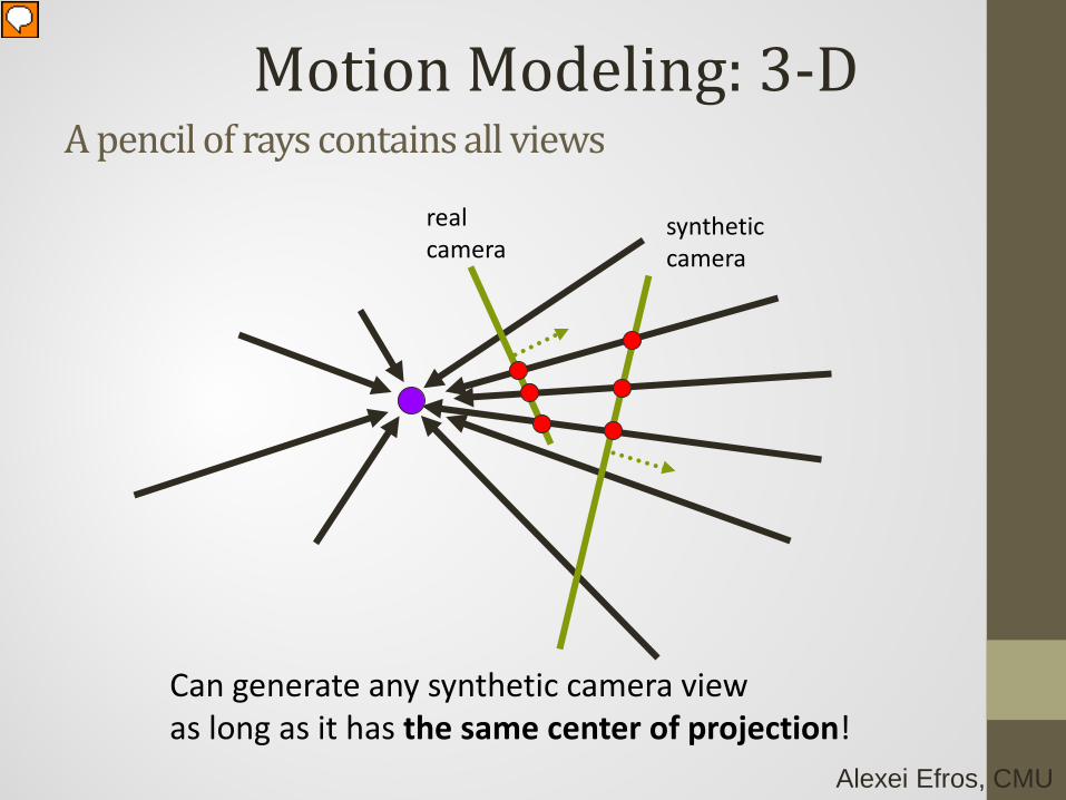
A pencil of rays contains all views

real camera

synthetic camera

Can generate any synthetic camera view as long as it has the same center of projection!

Alexei Efros, CMU

Motion Modeling: 3-D

Outline • Motivation • Stitching Steps

• Coordinate System and Motion Modeling • Alignment: Direct and Feature-based • Compositing

• Conclusions

Direct (Pixel-based) Alignment

Complexity of error metric depends on complexity of motion model

Determine Error Metric Use search technique to find possible alignments

Example of Simple Error Metric & Search Method • Maximum cross-correlation

• Do linear search over range of shifts in u to find maximum correlation

Feature-based approach 1. Detect local features 2. Extract feature descriptor 3. Match feature between two images 4. Estimate homography using RANSAC 5. Warping 6. compositing

http://www.di.ens.fr/willow/teaching/recvis10/assignment2/

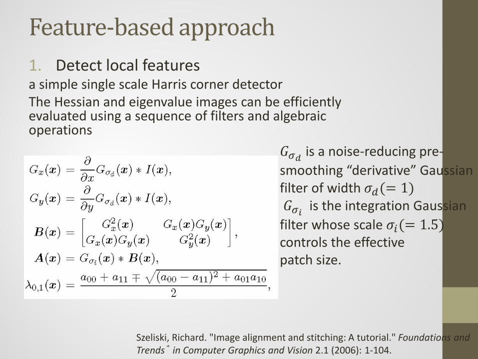
Feature-based approach 1. Detect local features a simple single scale Harris corner detector The Hessian and eigenvalue images can be efficiently evaluated using a sequence of filters and algebraic operations

Szeliski, Richard. "Image alignment and stitching: A tutorial." Foundations and Trends® in Computer Graphics and Vision 2.1 (2006): 1-104.

𝐺𝜎𝑑 is a noise-reducing pre-smoothing “derivative” Gaussian filter of width 𝜎𝑑(= 1) 𝐺𝜎𝑖 is the integration Gaussian filter whose scale 𝜎𝑖(= 1.5) controls the effective patch size.

Feature-based approach 1. Detect local features

Brown et.al, "Multi-image matching using multi-scale oriented patches." Computer Vision and Pattern Recognition, 2005. CVPR 2005. IEEE Computer Society Conference on. Vol. 1. IEEE, 2005.

𝑓𝐻𝐻 𝑥,𝑦 =det𝐴(𝑥,𝑦)𝑡𝑡 𝐴(𝑥,𝑦) =

𝜆1𝜆2𝜆1 + 𝜆2

• Interest point are located where corner strength is a local maximum in 3*3 neighbourhood

• Non-maximal supresion for spreading out interest points

Feature-based approach 2. Extract feature descriptor

Mikolajczyk et al, "A performance evaluation of local descriptors." Pattern Analysis and Machine Intelligence, IEEE Transactions on27.10 (2005): 1615-1630.

• 8x8 pixel patches patch around each detected feature to form a 64-dimensional descriptor (image intensity itself).

• sample from the larger 40x40 window to have a nice large blurred descriptor.

• bias/gain-normalize intensity. • Invariant to intensity change,

but sensitive to scale change, rotation, not a problem for the basic case.

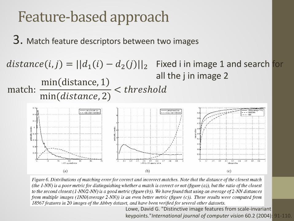
Feature-based approach 3. Match feature descriptors between two images

Lowe, David G. "Distinctive image features from scale-invariant keypoints."International journal of computer vision 60.2 (2004): 91-110.

𝑑𝑑𝑑𝑡𝑑𝑑𝑑𝑑(𝑑, 𝑗) = ||𝑑1(𝑑) − 𝑑2(𝑗)||2

match: min distance, 1min (𝑑𝑑𝑑𝑡𝑑𝑑𝑑𝑑, 2)

< 𝑡𝑡𝑡𝑑𝑑𝑡𝑡𝑡𝑑

Fixed i in image 1 and search for all the j in image 2

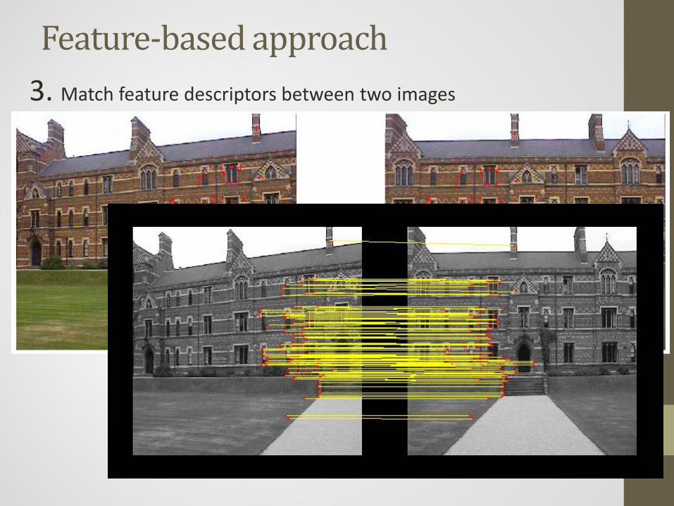
Feature-based approach 3. Match feature descriptors between two images

Feature-based approach 4. Estimate homography using RANSAC

note written by David Kriegman for Computer Vision I CSE 252A, UCSD, Winter 2007

𝐴𝑡 = 0 𝐴 = 𝑈Σ𝑉𝑇 𝑡 = 𝑣𝑛

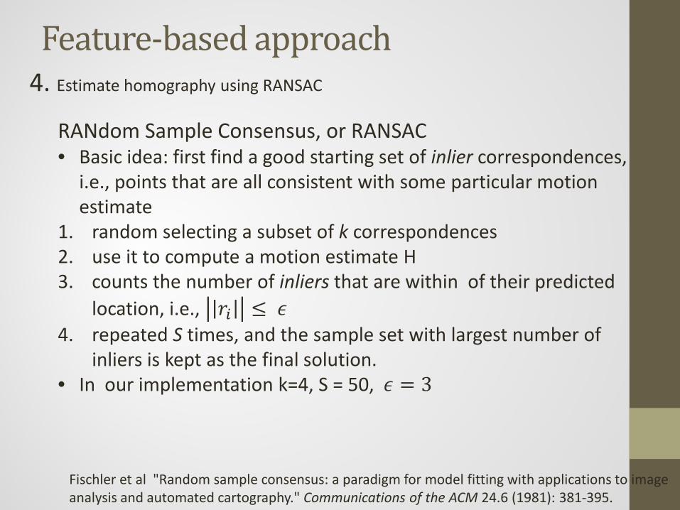
Feature-based approach 4. Estimate homography using RANSAC

RANdom Sample Consensus, or RANSAC • Basic idea: first find a good starting set of inlier correspondences,

i.e., points that are all consistent with some particular motion estimate

1. random selecting a subset of k correspondences 2. use it to compute a motion estimate H 3. counts the number of inliers that are within of their predicted

location, i.e., 𝑡𝑖 ≤ 𝜖 4. repeated S times, and the sample set with largest number of

inliers is kept as the final solution. • In our implementation k=4, S = 50, 𝜖 = 3

Fischler et al "Random sample consensus: a paradigm for model fitting with applications to image analysis and automated cartography." Communications of the ACM 24.6 (1981): 381-395.

Feature-based approach 4. Estimate homography using RANSAC

Note the robustness to pick out the real match features

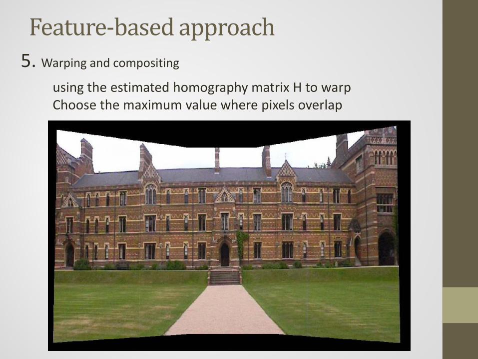
Feature-based approach 5. Warping and compositing

using the estimated homography matrix H to warp Choose the maximum value where pixels overlap

Feature-based approach 6. Speed up

Use the Adaptive Non-Maximal Suppression algorithm # of Features ~ 100 time: 8.97 s

Control (use all the features) # of Features ~ 5000 time: 128.85 s

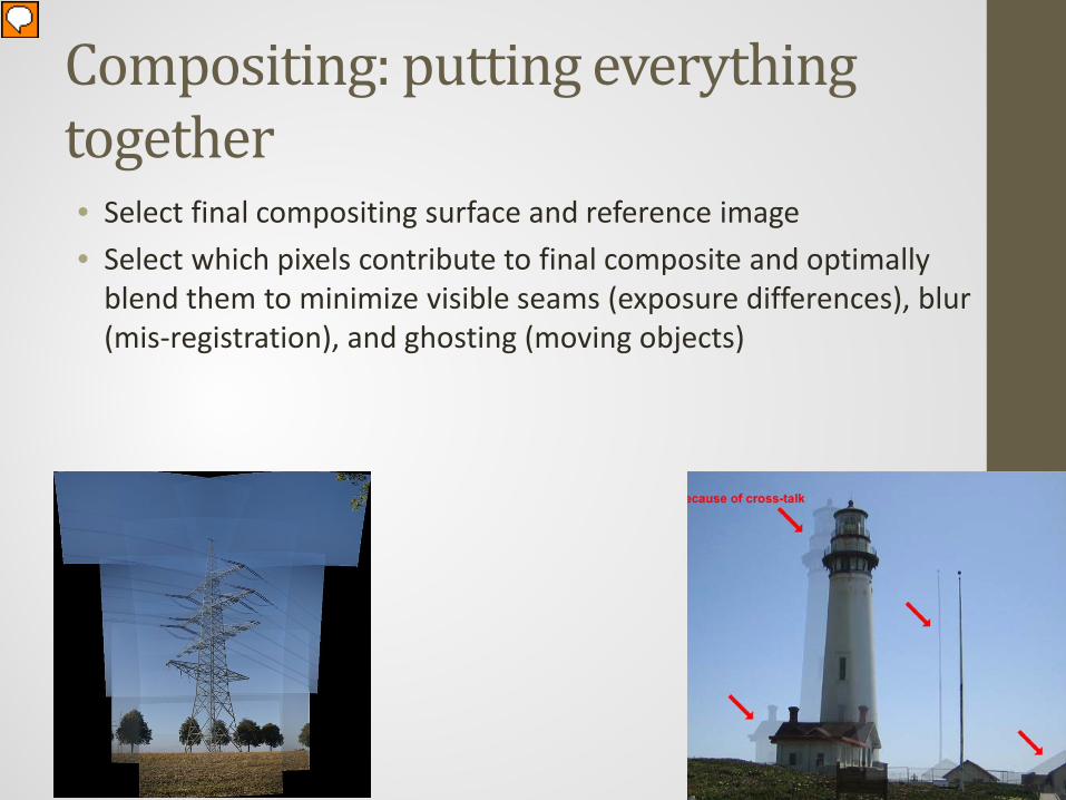
Compositing: putting everything together • Select final compositing surface and reference image • Select which pixels contribute to final composite and optimally

blend them to minimize visible seams (exposure differences), blur (mis-registration), and ghosting (moving objects)

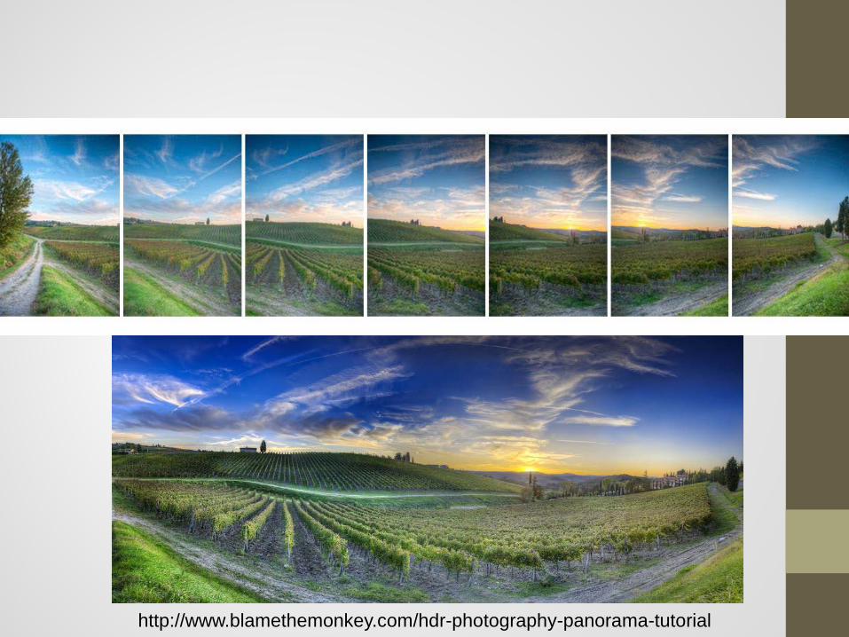
http://www.blamethemonkey.com/hdr-photography-panorama-tutorial

Summary • Image stitching • Choice of algorithms depends on complexity of image

differences • Trade off between robustness, accuracy, computation time