IMAGE SEQUENCE CLASSIFICATION VIA ANCHOR PRIMITIVES

by Gregory J. Clary

A dissertation submitted to the faculty of the University of North Carolina at Chapel Hill in partial fulfillment of the requirements for the degree of Doctor of Philosophy in the Department of Computer Science.

Chapel Hill

2003

Approved by

Advisor: Professor Stephen M. Pizer, Ph.D. Reader: Professor Stephen R. Aylward, Ph.D. Reader: Professor Steven W. Falen, M.D., Ph.D. Reader: Professor J.S. Marron, Ph.D. Reader: Dr. Krishna S. Nathan, Ph.D.

ii

© 2003 Gregory J. Clary

ALL RIGHTS RESERVED

iii

ABSTRACT GREGORY J. CLARY: Image Sequence Classification via Anchor Primitives

(Under the direction of Stephen M. Pizer, Kenan Professor)

I define a novel class of medial primitives called anchor primitives to provide a

stable framework for feature definition for statistical classification of image sequences of

closed objects in motion. Attributes of anchor primitives evolving over time are used as

inputs into statistical classifiers to classify object motion.

An anchor primitive model includes a center point location, landmark locations

exhibiting multiple symmetries, sub-models of landmarks, parameterized curvilinear

sections and relationships among all of these. Anchor primitives are placed using image

measurements in various parts of an image and using prior knowledge of the expected

geometric relationships between anchor primitive locations in time-adjacent images.

Hidden Markov models of time sequences of anchor primitive locations, scales and

nearby intensities and changes in those values are used for the classification of object

shape change across a sequence. The classification method is shown to be effective for

automatic left ventricular wall motion classification and computer lipreading.

Computer lipreading experiments were performed on a published database of

video sequences of subjects speaking isolated digits. Classification results comparable to

those found in the literature were achieved, using an anchor primitive based feature set

that was arguably more concise and intuitive than those of the literature. Automatic left

ventricular wall motion classification experiments were performed on gated blood pool

iv

scintigraphic image sequences. Classification results arguably comparable to human

performance on the same task were achieved, using a concise and intuitive anchor

primitive based feature set. For both driving problems, model parameters were tuned and

features were selected in order to minimize the classification error rate using leave-one-

out procedures.

v

To Julie, my first angel To Grandmother Clary, who blessed us with her outlook on life

To Grandmother Brown, who blessed us with her example

vi

ACKNOWLEDGEMENTS

I would like to express my sincere appreciation to all of the people who have

supported this research and this effort.

I begin by thanking Dr. Steve Pizer, whose patience and encouragement are truly

second to none. Dr. Pizer has been extremely supportive of my unusual process with its

highs and lows of various kinds, and I would not have finished this work without his

dedicated efforts. I would like to thank the other members of my dissertation committee,

Dr. Stephen Aylward, Dr. Steven Falen, Dr. J.S. Marron, and Dr. Krishna S. Nathan, all

of whom provided extremely useful input on both the document and the research. I

appreciate Krishna Nathan’s effort and willingness to travel from Zurich to the

dissertation defense.

I thank other friends in the Computer Science department of UNC for various

forms of support including Delphine Bull, Janet Jones, Stephen Aylward, Gary Bishop,

David Harrison, Leandra Vicci and Russ Taylor.

I thank members of the Radiology department of UNC for their support including

the late Dr. J. Randolph Perry, Rick Lonon, Dr. Stephen Aylward and Dr. Steven Falen.

A special thanks to Dr. Dan Fritsch and Yoni Fridman.

I would like to thank my former colleagues of IBM Research who provided

inspiration and friendship through many years including Jay Subrahmonia, Rob Stets,

Gene Ratzlaff, Tom Chefalas, and Krishna Nathan. I thank Krishna Nathan for having

very high standards that lead to valuable work product.

vii

I appreciate the support of my colleagues at Mi-Co who have taken on numerous

extra burdens as a result of my focus on this work in its later stages. They include Jim

Clary, Carolee Nail, Barrett Joyner, Jason Priebe, Chris DiPierro, David Nakamura,

Joseph Tate, Bill Henthorn and Bill Backus. You are a truly great team.

I thank my parents for more influence, goals, achievements, standards, values, and

examples than this space allows me to describe. Words cannot do their contributions to

my life justice.

Finally, I thank Julie, Mollie and James for their patience, support and most of all,

their love. And I thank God for His grace and mercy.

viii

TABLE OF CONTENTS

Page

LIST OF TABLES.........................................................................................................xi LIST OF FIGURES ..................................................................................................... xii Chapter 1. Introduction.................................................................................................................1 1.1. Contributions..................................................................................................9

2. Left Ventricular Regional Wall Motion Analysis.....................................................13 3. Computer Lipreading................................................................................................22 4. Background on Image Segmentation and Statistical Classification of Time Sequences...............................................................................................31 4.1. Deformable Model Based Segmentation Methods ......................................32 4.1.1. Landmark Methods ..........................................................................33 4.1.2. Boundary Based Methods for Segmentation ...................................35 4.1.3. Atlas Based Methods .......................................................................36 4.1.4. Deformable M-reps..........................................................................36 4.2. Hidden Markov Models ...............................................................................41 4.3. Summary ...................................................................................................43 5. Image Sequence Classification via Anchor Primitives.............................................47 5.1. Correspondence and Deformable Models....................................................47 5.2. Anchor Primitive Definition.........................................................................49

ix

5.3. Anchor Primitive Representing the Left Ventricle ......................................53 5.4. Approach to Fitting Anchor Primitives to the Left Ventricle ......................56 5.4.1. Objective Function...........................................................................57 5.4.2. Image Match Function .....................................................................57 5.4.3. Measuring Boundariness..................................................................58 5.4.4. Geometric Penalty Function for Left Ventricle Anchor Primitive..........................................................................................59 5.5. Anchor Primitive Based Segmentation of Lip Image Sequences ................60 5.5.1. Image Match Terms .........................................................................61 5.5.2. Geometric Penalty Terms ................................................................62 5.5.3. Tracking Approach for Lip Image Sequences .................................62 5.6. Classification of Image Sequences Using Anchor Primitives .....................64 6. Results and Conclusions ...........................................................................................66 6.1. Left Ventricular Regional Wall Motion Analysis........................................67 6.1.1. Anchor Primitive for Left Ventricle ................................................68

6.1.2. Left Ventricle’s Statistical Features Implied by the Anchor

Primitive Model ..............................................................................70 6.1.3. Left Ventricular Image Data ............................................................70 6.1.4. Semi-Automatic Segmentation of Left Ventricular Image Sequences........................................................................................79

6.1.5. Feature Selection and Hidden Markov Models for Left

Ventricular Regional Wall Motion Classification ..........................80 6.1.6. Comparison of Left Ventricular Classification Results to Other Work .................................................................................83 6.2. Computer Lipreading...................................................................................84 6.2.1. Anchor Primitive for Lips................................................................84

x

6.2.2. Lip’s Statistical Features Implied by the Anchor Primitive

Model ..............................................................................................85 6.2.3. Lip Image Data ................................................................................86 6.2.4. Semi-Automatic Segmentation of Lip Image Sequences ................87

6.2.5. Feature Selection and Hidden Markov Models for

Computer Lipreading......................................................................89

6.2.6. Comparison of Lip Image Sequence Classification Results to Other Work .................................................................................90

6.3. Conclusions Regarding Anchor Primitives..................................................92 6.4. Contributions................................................................................................96 7. Future Work ............................................................................................................100 BIBLIOGRAPHY.......................................................................................................109

xi

LIST OF TABLES

Table 6.1 Attributes of left ventricle anchor primitive model used as features for classification..........................................................................................70

Table 6.2 Cases where a consensus was reached by two human experts on

apical regional wall motion.........................................................................77

Table 6.3 Number of classification errors for each individual left ventricle anchor primitive feature ..............................................................................81

Table 6.4 Number of classification errors using a greedy selection of features based on Table 6.3 ......................................................................................81

Table 6.5 Number of classification errors for various combinations of features for various numbers of states per hidden Markov model ...........................83

Table 6.6 Features used for lip image sequence classification ....................................86 Table 6.7 Number of classification errors for each individual lip anchor primitive feature..........................................................................................90 Table 6.8 Number of classification errors using a greedy selection of features based on Table 6.7 without considering S2 and S4 ....................................90

xii

LIST OF FIGURES

Figure 2.1 A schematic of the human heart .................................................................14 Figure 4.1 A medial primitive in a 2D image object ...................................................37 Figure 4.2 Blood pool frames ......................................................................................38 Figure 4.3 A two state hidden Markov model .............................................................41

Figure 5.1 Medial primitives, including end primitives, may “slide” .........................48

Figure 5.2 A schematic of a salamander and its anchor primitive model....................51

Figure 5.3 The anchor primitive for left ventricular segmentation..............................54

Figure 5.4 The anchor primitive a values ....................................................................55

Figure 5.5 The distance S2 between the anchor primitive location and

the apex ......................................................................................................56

Figure 5.6 The normals to a partial ellipse determine a kernel area ............................58

Figure 5.7 Anchor primitive representing the lips .......................................................61

Figure 6.1 The regions of the left ventricle from a modified left anterior oblique viewpoint.......................................................................................68

Figure 6.2 The anchor primitive for left ventricular segmentation..............................69 Figure 6.3 An example ECG gated blood pool equilibrium 32 frame

image sequence ..........................................................................................71

Figure 6.4 P(W|A) for various values of P(R) .............................................................74 Figure 6.5 P(W|A) for various values of p...................................................................76 Figure 6.6 An example of automatic segmentation of the left ventricle

in an image sequence .................................................................................79

Figure 6.7 Schematic of the Lip Anchor Primitive......................................................85

xiii

Figure 6.8 An example of a sequence from the Tulips 1 lip image sequence database.......................................................................................................87

Figure 6.9 Anchor primitive based semi-automatic segmentation of a lip

image sequence “four”...............................................................................88

Figure 6.10 Comparison between numbers of errors and numbers of features.....................................................................................................91

Chapter 1

Introduction

In this the technology age, sequences of images are commonly captured and

displayed. Capture mechanisms include video and motion picture film cameras, medical

imaging devices such as those that image the heart, and radar. Many image sequences

portray objects in motion that undergo shape changes. Machines of the twenty-first century

will usefully automatically classify the motion of objects in image sequences. Example

applications will include security and medical diagnosis. Imagine a security system where

the act of shoplifting is automatically recognized by machines. Even imperfect systems

would save retailers millions of dollars! In an imperfect system, where the probability of

false alarms is non-zero, human security personnel could review recordings of acts that are

considered suspicious by the system and decide whether or not to take further action.

As another example application, consider a “hands-free” dialing system for a mobile

telephone unit in an automobile. Various noise types may corrupt an acoustic signal in the

car environment, including the sounds from passing cars, the engine, the fan, the tires, the

voices of passengers, and the radio to name a few. A small camera can be mounted

unobtrusively on the ceiling or mirror and focused on the driver. Video signals from the

camera can be sent to a SmartPhone or similar device to aid in the recognition of spoken

digits and commands.

2

Most automatic speech recognition research has focused on using the acoustic signal

to recover the linguistic information intended by the speaker. Recognition using the acoustic

signal has proven to be extremely difficult in noisy environments, where the speech portion

of the acoustic signal is distorted by background interference, possibly from a variety of

sources. Many types of noise are mid to high frequency in nature and thus interfere with the

mid to high frequency components of the acoustic signal. (The low frequency content of the

acoustic signal is often largely unaffected by noise.) The mid to high frequency content of

the acoustic signal is directly related to the positions of articulators like the lips, teeth and

tongue. Obviously, acoustic noise interference does not impact a video sequence of the

speaker. The positions of the lips, teeth and tongue are often clearly shown in such a

sequence.1 Thus, a video signal can be used effectively to augment the acoustic signal in

automatic speech recognition systems.

This dissertation explores a novel method for the classification of object shape

changes in image sequences. The method describes shape changes in image sequences

numerically and assigns the shape changes to categories.

At a high level, the approach to image sequence classification taken is to find the

object of interest in each frame of the image sequence, generate a numerical description of its

shape, accumulate the numerical descriptions of the object shape in each frame over time and

pass the numerical descriptions on to a statistical classifier. This work focuses on finding the

object in each frame (segmentation and tracking) and describing its shape numerically

(feature extraction). For a statistical classification system, numerical descriptions of shape

should be 1) concise enough to allow computational efficiency of statistical classification and

3

accurate model parameter estimation and 2) have the right precision to allow accurate

classification of data not previously encountered.

Statistical classifiers compute distances between models and new inputs

(equivalently, they compute the a posteriori probabilities of new inputs). The computational

expense of the distance calculations depends on the metric used but can increase as the

square of the number of extracted features. Thus, for computationally efficient statistical

classification, the number of extracted features should be kept small; that is, feature vectors

that describe object shape should be concise. Numerous concise ways to describe shape have

been proposed and explored in the literature, including Fourier coefficients of the object’s

intrinsic function and moments. Someone new to the field might be tempted to describe an

object’s shape in a digital picture by listing all of the pixels that fall within the object, but of

course this method is not at all concise. Duda and Hart put it well, “…completely specifying

the points in the figure does violence to our intuitive notion that a description of a complex

thing should be simpler in some sense than the thing being described.”2

Beyond computational efficiency, a further motivation for finding concise feature sets

is to allow creation of representative statistical models based on a finite set of training data,

as explained by the following argument. In statistical classifiers, model parameters such as

mean vectors and covariance matrices are estimated from training data. According to the

Laws of Large Numbers, sample based estimates of distribution parameters approach the true

distribution parameters as the sample size increases. The implication for statistical

classification is that more training samples result in more accurate model parameter

estimates. Accurate estimates of appropriately selected model parameters yield high

classification accuracy. In many cases, however, training data is scarce. Thus, a researcher

4

using a statistical classifier is motivated to try to estimate fewer well-chosen parameters, in

order to better estimate them and achieve better classifier accuracy.

Whether or not the features have the right precision is judged in part by estimates of

classification accuracy, obtained by presenting data to the classifier that was not presented

during training. Classifier performance is tuned by varying the number and choice of

parameters and using a technique like cross-validation, in order to avoid “over-training” to a

particular training set. The result of over-training is that the classifier has limited

generalization capability. That is, when an over-trained classifier sees an input not presented

during training, it is less likely to classify it correctly than another classifier that has not been

over-trained to the training set.

Intuitively, the challenge is to generate from image data a numerical description of

the object of interest in the image that is concise (like “cow” for the main object in a

photograph of a cow) but also has the right amount of precision for classification purposes.

“Right amount” is problem dependent. For example, if cows are to be classified into various

breeds (categories) like Holstein and Guernsey, more precise descriptions are needed. Such

descriptions could include “cow has black spots on a white background” or “cow is

completely brown.”

Methods previously applied by computer image analysts to shape description suffer

from sensitivity to subtle intensity variations within the object of interest, and many are not

invariant to translation, rotation and zoom. An intuitive way to think of invariance is to again

imagine a photograph that pictures a cow. Now imagine a second photograph that was taken

when the photographer stepped toward the cow (zoomed in), took a step to the right

(translated the camera) and tilted the camera (thereby rotating the cow in the photograph).

5

The description of the object of interest in the second photograph is invariant to the described

transformations in the sense that it is “cow” regardless of the fact that translation, rotation

and zooming took place.

Most of the methods for numerically describing object shape depend on knowing the

object’s boundaries as a prerequisite. Typically, they depend on a traditional boundary

finding technique such as a gradient based one, which is known to cause difficulty when

there is image noise or perturbations.

A method that overcomes some of the difficulties of other shape description methods

is based on the principle that a precise and concise way to describe an object is by describing

its middle or “medial track” and width along the middle. There is psychophysical evidence

to suggest that a fundamental mechanism underlying human object perception (and therefore

shape description) is the association of opposing boundaries, that is, the performance of

medial analysis.3 By the performance of medial analysis, a human or machine can concisely

summarize the shape of an object. In this dissertation, attributes of this medial summary

information are used as features for the classification of object shape change in image

sequences. Intuitively, a system that performs medial analysis assigns the position of an

object’s middle by “linking” boundaries, that is, gathering evidence for opposing boundaries.

Based on evidence of a boundary in one part of an image and evidence for a boundary in

another part of an image, the system assigns a “medial primitive” to a location in the image

between the two boundaries.

A way of describing an object’s shape and capturing its figural geometry was first

proposed by Blum4 and is known as the medial axis transform. The medial axis of an object

is a locus of middle (medial or skeletal) points and a radius (“half-width”) associated with

6

each of the middle points. The medial axis description of an object is complete in the sense

that an object’s boundary can be reconstructed if its medial points and associated radii are

known. The locus of medial points was defined by Blum to be the locus of centers of disks

that are tangent to the object boundary in two places. The associated radii are the radii of the

doubly tangent disks. Stephen Pizer and his colleagues at the University of North Carolina at

Chapel Hill (UNC) have introduced ways of finding medial loci in images in a manner which

is insensitive to image noise and small perturbations in the object’s boundary and which does

not depend on knowing the object’s boundary as a prerequisite. More will be said about the

UNC method in Chapter 4.

The central thesis of the dissertation is that novel medial representations called anchor

primitives are useful as a basis for feature extraction for object shape sequence classification,

because the resulting features are precise enough for classification and concise enough to

allow computational efficiency of statistical classifiers and accurate model parameter

estimation. An anchor primitive models only salient parts of an image object, and it uses

symmetries advantageously to produce a compact representation of the image object. The

anchor primitive based method is a general framework for image segmentation and statistical

feature definition. The framework is evaluated on 2D image segmentation and image

sequence classification problems in this work.

Image sequence classification problems considered here include left ventricular

regional wall motion classification and computer lipreading. What left ventricular wall

motion classification and computer lipreading have in common is that useful automatic

classifications can be made from 2D image sequences. In addition, the image sequences

capture a body in motion that can be viewed as consisting of a single figure. That is, within

7

each image of a sequence, the boundary of the object of interest, namely the left ventricle or

the mouth, is closed or nearly closed and there is a medial axis that provides an adequately

good approximation of the object. The medial topology of the object of interest is fixed over

the sequence. Although the high-level approach for image sequence classification described

in this dissertation is general, results will be demonstrated only for single figure objects that

are not occluded. Other problems of interest in the computer vision community include

classification of the motion of multi-figure objects that can be occluded or self-occluded, for

example, classification of human activities like walking or hand gestures (or the unfortunate

shoplifting activity!).

The focus of the dissertation is on representing image objects for statistical

classification rather than the search for engineering solutions to the example problems of left

ventricular wall motion classification and computer lipreading. Chapter 2 and Chapter 3

provide further background on these problems. Brief background on the driving

classification problems is given here.

The left ventricular chamber is of primary interest because it is the heart’s

workhorse—it contracts to pump oxygen-rich blood to the body. Because of its crucial role

in the circulatory system, analysis of the motion of its walls is sometimes undertaken as an

aid to heart disease diagnosis. Current practice for clinical interpretation relies on subjective

assessments based on observer training. Automatic classification of left ventricular regional

wall motion would 1) enable the computer as an observer in order to save costly human

observer time and 2) improve reproducibility and reliability.

The region of the left ventricular wall found roughly in the direction of the human

feet is known as the apex. Automatic classification of left ventricular apical motion into two

8

categories, “normal apical motion” and “abnormal apical motion,” is undertaken in this

research. Results indicate that wall motion classification using features based on attributes of

a novel anchor primitive model is efficient in terms of the number of features required by an

employed statistical classifier.

Automatic classification of the spoken digits “one” through “four” from video signals

is also undertaken in this research. Such computer lipreading is useful in automatic

recognition environments where the acoustic signal is corrupted by noise. Other researchers

have demonstrated that 1) for the studied digit recognition task high recognition accuracy is

achievable5 and 2) the errors made by audio and video based recognition schemes are

complementary.6 This dissertation will define an image sequence processing and

classification system that could be used in an audio-visual speech recognition system. The

defined anchor primitive based system is compared to systems of the literature that were

evaluated on the same spoken digit task and is found to offer arguably more concise and

intuitive statistical features than those of previous systems while maintaining comparable

classification accuracy.

At a high level, the approach taken to image sequence classification is typical. First,

images are segmented to find the object of interest. Features are extracted which represent

shape and shape change aspects of the segmented object. These features are accumulated

over time and used as input into a classifier that assigns a category to the image sequence.

At a more specific level, models that consist of my anchor primitive are used to

segment the images. Attributes of these models are used as features. They include distances

between model points; local estimates of width and radius of curvature; and the inter-frame

changes in those values. The features are inputs to a statistical classifier which outputs a

9

category assignment like “abnormal apical motion” in the case of the left ventricular wall

motion analysis problem or one of the digits “one” through “four” in the case of the computer

lipreading problem. It will be argued that the anchor primitive framework has the following

advantages:

• An anchor primitive uses a smaller number of parameters to represent an

image object than would be used by alternative representations.

• Anchor primitive distance attributes and changes in those distances when

captured over time can be used to adequately describe image object motion.

• Anchor primitives provide accurate statistical features for image sequence

classification.

• Anchor primitives provide concise features for statistical classification.

• Their attributes often have intuitive meaning, e.g., half-width of the mouth or

half-length of the long axis of the left ventricle.

• Anchor primitives can provide a rich statistical feature set.

• Anchor primitives are able to delineate image objects in noisy data.

1.1 Contributions

The contributions of the dissertation are the following:

• I describe a novel medial primitive called an anchor primitive. The anchor

primitive can represent boundary parts of an object with parametric curves.

There are symmetric relationships between represented parts. The anchor

primitive includes an object “center” location, information about locations of

the parts, and curve parameters. It will be shown that anchor primitives allow

consistent model placements relative to salient image object features that are

10

needed for accurately defining statistical features for image sequence

classification. Certain image object features that are found in every example

image object across a population are said to “correspond.” The anchor

primitive is a correspondence maintaining primitive placed in each frame of

an image sequence using the continuity of the sequence. Anchor primitives in

image sequences effectively generate shape parameter sequences that describe

object motion. Thus, attributes of anchor primitives can be effectively used as

features for image sequence classification.

• I show that anchor primitives supply features for statistical classification that

are intuitive and easy to compute.

• I introduce a method for classification of object shape change in image

sequences that combines anchor primitive attributes and hidden Markov

models.

• I demonstrate that anchor primitive attributes are useful for left ventricular

wall motion classification.

• I demonstrate that anchor primitive attributes are useful for computer

lipreading of spoken digits.

• I select particular anchor primitive attributes as features for statistical

classifiers.

The remainder of the dissertation is structured as follows. Chapter 2 reviews previous

approaches to left ventricular regional wall motion analysis and classification. Chapter 3

summarizes previous work on the computer lipreading problem. Chapter 4 presents the

theoretical details of previously employed (by this author and other authors) deformable

11

models and Hidden Markov Models. Chapter 5 presents the proposed anchor primitive based

methodology in detail with emphasis on the novel contributions of the work and theoretical

justifications for them. Chapter 6 gives evaluations of the methodology for left ventricular

apical motion classification and results for computer lipreading of the digits “one” through

“four.” Chapter 6 also presents those anchor primitive attributes selected as features for the

statistical classifiers. Chapter 6 finishes by discussing the results and drawing conclusions.

Chapter 7 presents ideas for future work.

12

1. N.M. Brooke, “Talking Heads and Speech Recognizers That Can See: The

Computer Processing of Visual Speech Signals,” in Speechreading by Humans and Machines: Models, Systems, and Applications, D.G. Stork and M.E. Hennecke, ed., Berlin: Springer-Verlag, 1996, pp. 351-371.

2. R.O. Duda and P.E. Hart, Pattern Classification and Scene Analysis, New York:

John Wiley & Sons, 1973, p. 341. 3. C.A. Burbeck, S.M. Pizer, B.S. Morse, D. Ariely, G.S. Zauberman, and J.P.

Rolland, “Linking object boundaries at scale: a common mechanism for size and shape judgments,” Vision Research, Vol. 36, pp. 361-372.

4. H. Blum, “A Transformation for Extracting New Descriptors of Shape,” in

Symposium on Models for Perception of Speech and Visual Form, W. Whaten-Dunn, ed., Cambridge, MA: MIT Press, 1967, pp. 362-380.

5. J. Luettin and N.A. Thacker, “Speechreading using Probabilistic Models,”

Computer Vision and Image Understanding, Vol. 65, No. 2, 1997, pp. 163-178. 6. E.D. Petajan, “Automatic Lipreading to Enhance Speech Recognition,” Ph.D.

thesis, Univ. of Illinois, Urbana-Champaign, 1984.

Chapter 2

Left Ventricular Regional Wall Motion Analysis

Recent cardiac image analysis work has focused on 3D image acquisition modalities

and analysis techniques. Frangi, Niessen, and Viergever give an excellent overview of model

based 3D cardiac image analysis approaches.1 In addition, recently, an issue of IEEE

Transactions on Medical Imaging was devoted entirely to 3D cardiovascular image analysis.2

The methods studied in this dissertation will apply to 3D image analysis, but their efficacy is

demonstrated herein on 2D images.

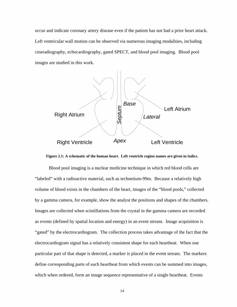
The left ventricle and the names of certain of its walls and regions are illustrated in

Figure 2.1. As was stated, because of the left ventricle’s crucial role in the circulatory

system, analysis of the motion of its walls is sometimes undertaken as an aid to heart disease

diagnosis, including evaluation of coronary artery disease, infarcts and ischemia. In addition,

certain chemotherapy regimens are toxic to the heart muscle. Such regimens are commonly

administered until wall motion analysis shows that muscle performance is significantly

degrading. Abnormal wall motion is most easily observed when a patient is subjected to

stress such as exercise. According to one source,3 “exercise-induced wall motion

abnormalities occur in approximately 50 percent of patients with coronary artery disease

without prior myocardial infarction.” That is, stress-induced wall motion abnormalities can

14

occur and indicate coronary artery disease even if the patient has not had a prior heart attack.

Left ventricular wall motion can be observed via numerous imaging modalities, including

cineradiography, echocardiography, gated SPECT, and blood pool imaging. Blood pool

images are studied in this work.

Left Ventricle

Left Atrium

Right Ventricle

Right Atrium

Apex

Base

LateralS

eptu

m

Figure 2.1: A schematic of the human heart. Left ventricle region names are given in italics.

Blood pool imaging is a nuclear medicine technique in which red blood cells are

“labeled” with a radioactive material, such as technetium-99m. Because a relatively high

volume of blood exists in the chambers of the heart, images of the “blood pools,” collected

by a gamma camera, for example, show the analyst the positions and shapes of the chambers.

Images are collected when scintillations from the crystal in the gamma camera are recorded

as events (defined by spatial location and energy) in an event stream. Image acquisition is

“gated” by the electrocardiogram. The collection process takes advantage of the fact that the

electrocardiogram signal has a relatively consistent shape for each heartbeat. When one

particular part of that shape is detected, a marker is placed in the event stream. The markers

define corresponding parts of each heartbeat from which events can be summed into images,

which when ordered, form an image sequence representative of a single heartbeat. Events

15

from irregular beats are ignored, and the fact that only a small amount of radioactive material

is introduced into the bloodstream is overcome by the gating and summing process.

“Equilibrium images” are captured when the radioactive material is uniformly distributed

throughout the blood stream. This research uses modified left anterior oblique (MLAO)

gated blood pool equilibrium image sequences from patient studies. The MLAO view is

used since it most clearly shows the left ventricular chamber.

Wall motion can be classified as normokinetic, mildly hypokinetic, moderately

hypokinetic, severely hypokinetic, akinetic or dyskinetic, that is, regions of the left

ventricular walls can exhibit various types and degrees of motion abnormalities. Current

practice for clinical interpretation relies on subjective assessments based on observer

training, which can sometimes result in significant intra-observer and inter-observer

variability. Reliable, automatic classification of left ventricular (LV) regional wall motion

would 1) enable the computer as an observer in order to save costly human observer time and

2) improve reproducibility and reliability. Presented in this work is a model based approach

to automatic left ventricular wall motion classification.

A commonly used method for quantifying LV regional wall motion is the “centerline

method” developed by Sheehan et al.4 This 2D method measures motion along chords

perpendicular to a “centerline.” The centerline is a curve that is halfway between the LV

end-diastolic and end-systolic boundary contours. The boundary contours are typically

chosen manually. The method does not require localization of the apex. Sheehan et al.

showed that the centerline method distinguishes normal patients from patients with

ventricular wall motion abnormalities associated with coronary artery disease. The motion

16

measurement it provides correlates well with the severity of stenosis, and the mean wall

motion abnormality it provides correlates well with area ejection fraction.

One example of early work to automatically classify LV regional wall motion is the

work by Sychra, et al.5 They form “Fourier Classification Images” by harmonic analysis of

pixel time activity curves from cardiac nuclear medicine images as a basis for feature

computation, Fisher’s linear discriminant analysis of the features, and Gaussian modeling of

8 wall motion classes. Wall motion classes are normal 1, normal 2, mildly hypokinetic,

hypokinetic, hypokinetic-akinetic, akinetic, akinetic-dyskinetic, and dyskinetic. Each pixel

in Sychra’s images is assigned a wall motion class based on analysis of its time activity

curve. They define “acceptable agreement” with the consensus of sequence analysis by

physicians as differing from the consensus by one class or less. With this definition of

“acceptable agreement,” they achieved an average of 86% pixel accuracy for normal classes

and 73.3% pixel accuracy for hypokinetic classes on their training set. They analyzed a total

of 70 cardiac studies.

More recently, Nastar and Ayache suggested a 3D model that they claim can be

applied to automatic diagnosis of heart disease.6 They define a deformation spectrum based

on modal analysis of a physically based deformable surface. They use the deformation

spectrum to compare deformations.

Gated myocardial perfusion SPECT imaging is commonly used to quantify left

ventricular performance, myocardial perfusion and regional function. Global measures of

performance accurately attainable from cardiac gated SPECT include left ventricular ejection

fraction, end-diastolic chamber volume and end-systolic chamber volume. Local

quantification of wall motion and wall thickening is possible as well. In addition, gated

17

SPECT can provide 3D visualizations of left ventricular wall motion.7 Software that

facilitates myocardial perfusion SPECT analysis and interpretation has been developed by

Emory University, Cedars-Sinai Medical Center, and the University of Michigan and has

been licensed to a number of major companies.

Automatic classification of LV regional wall motion has been attempted before by

Tsotsos using his ALVEN system.8 A description of ALVEN was first published in

Tsotsos’s dissertation in 1980. Other descriptions of the ALVEN system can be found in

Tsotsos.9,10,11

ALVEN used images obtained by left ventricular angiography, a process which was

state-of-the-art at that time, but suffered from limitations. Angiographic images are collected

by taking conventional X-ray images of a radio-opaque dye injected through a catheter into

the desired location. The catheter is inserted into an artery in the upper arm or upper leg, and

guided through the aorta into the area to be imaged, which may be one of the chambers of the

heart or any of the coronary arteries.

ALVEN is a system that produces output corresponding to the active and most certain

hypotheses of a knowledge base. Much of the terminology used to describe the hypotheses

and organization of the knowledge base is the same as that used to describe modern object-

oriented programming (e.g., “instance-of,” “aggregation,” “inheritance”) suggesting that a

modern object-oriented language might be used to straightforwardly implement the

knowledge base. Which hypotheses are activated (i.e., which objects are instantiated) is

determined using rules on image and inter-image descriptions. A relaxation labeling

procedure, which limits the search space based on active hypotheses pertaining to the motion

of the ventricle, is used to find boundaries of the ventricle. For example, if “contract” is an

18

active hypothesis, the speed and direction of contraction calculated from previous frames can

limit the area in the current frame in which to search for the boundaries. If the boundaries

are not found, the constraints on the search space can be relaxed by using a parent of the

hypothesis. For example, “beat” might be a parent of “contract” and “expand,” so speeds and

directions for both contraction and expansion could define a search space. A less constrained

default search is used if the more constrained one(s) fail(s) to find an appropriate boundary.

Low-level image and inter-image descriptions are produced from the boundaries.

Hypotheses are activated according to the descriptions. Hypotheses are ranked by certainty

factor. Certainty factors are initialized according to a simple scheme (for example, if one

hypothesis is active and causes another to become active, the two may share equally the

certainty factor of the first). The certainty factors are updated using a relaxation labeling

procedure introduced by Zucker.

Most of Tsotsos’s reported results pertain to the analysis of the dynamics of

implanted Tantalum markers.5 Markers were implanted in the left ventricular wall of patients

who had undergone coronary bypass surgery. Films of the left ventricle and the markers in

motion allowed the evaluation of the effectiveness of the surgery and drug interventions.

Nine markers were implanted around the left ventricular wall and two on the aortic valve

edges. After hypotheses guided image analysis (described above) using a modified Marr-

Hildreth operator to extract the markers from the images, low-level image and inter-image

descriptions were produced. Low-level image descriptions included “major and minor axes,

volumes, 2D areas of segments, segmental volume contributions, circumferential dimensions,

and changes in radial axis lengths.” Low-level inter-image descriptions included “relative

directions of motion and rates of change.” Rules on the image and inter-image descriptions

19

caused activation of hypotheses corresponding to anomalies and their degrees like

“asynchrony, hypokinesis, dyskinesis, too slow or fast rate of change of volume with respect

to LV phase, or too long or short phase duration.” In Tsotsos5, an example left ventricle that

was judged by a radiologist to exhibit hypokinesis of the anterior segment is given. ALVEN

gave output for each of the markers, segments, and left ventricle that included a “descriptive

term, possible referent, quantitative values, and a time interval or instant.” HYPOKINESIS

is a descriptive term corresponding to one of the motion hypotheses. Quite a number of

HYPOKINESIS instances were reported by ALVEN. Most were for the anterior segment, in

agreement with the radiologist’s opinion.

To summarize ALVEN’s massive textual output, a summary graphic display was

developed. Time was presented on the horizontal axis, marker and segment index were

presented on the vertical axis, and shading indicated how the segment was moving (inward,

outward, not at all, and degree of hypokinesis if present). Tsotsos concluded that for several

studied cases, ALVEN gave output that was more detailed than, but still consistent with, the

radiologist’s assessment.

Left ventricular regional wall motion classification was chosen in this work as a

driving problem for developing and testing a new method for classifying non-rigid object

motion in image sequences. The previously described methods of Tsotsos and Sychra et al.

operate using a knowledge based or pixel time activity curve based approach to the problem.

According to Wechsler, knowledge based computational vision systems suffer because they

depend on knowledge that “is empirical, narrowly focused, involves a large number of

heuristic rules of thumb, and cannot be easily extended.”12 Pixel based methods cannot

handle aspects of cardiac motion like global translation and twisting of the heart during its

20

beating, because those global motion effects introduce activity into a pixel from multiple

anatomical locations. Model based approaches to cardiac analysis and segmentation

overcome these difficulties and are currently popular. This work introduces a model based

approach to cardiac image segmentation based on anchor primitives. The anchor primitive

models yield features in each frame, and thus sequences of feature vectors across time, that

have intuitive meaning and are easy to compute. Sequences of feature vectors are often

classified using hidden Markov models, because of their robust statistical nature and their

ability to capture time dependence in a way that is representative of a training set, rather than

based on ad hoc rules. Hidden Markov models allow modeling of non-stationary stochastic

processes and model feature changes that may vary in duration across time. This work

introduces a hidden Markov model based classification approach using anchor primitive

implied features. Sychra achieved about 80% classification accuracy (70 cases) on his

training set when distinguishing normal motion from hypokinetic motion. In a comparable

task in this work, 80% classification accuracy (25 cases) is achieved when distinguishing

normal motion from abnormal motion in a leave-one-out analysis.

The method developed in this work for regional wall motion classification is

presented in Chapter 5. Chapter 3 gives background information on the other motivating

image sequence classification problem studied in this work, computer lipreading.

21

1. A.F. Frangi, W.J. Niessen, and M.A. Viergever, “Three-Dimensional Modeling

for Functional Analysis of Cardiac Images: A Review,” IEEE Transactions on Medical Imaging, Vol. 20, No. 1, Jan. 2001.

2. A.F. Frangi, D. Rueckert, and J.S. Duncan, “Three-Dimensional Cardiovascular

Image Analysis,” IEEE Transactions on Medical Imaging, Vol. 21, No. 9, Sept. 2002. 3. E.G. DePuey, “Evaluation of Ventricular Function,” in Clinical Practice of

Nuclear Medicine, A. Taylor and F.L. Datz, ed., New York: Churchill Livingstone, 1991, p. 72.

4. F.H. Sheehan, E.L. Bolson, H.T. Dodge, D.G. Mathey, J. Schofer, and H.W.

Woo, “Advantages and applications of the centerline method for characterizing regional ventricular function,” Circulation, Vol. 74, No. 2, Aug. 1986.

5. J.J. Sychra, D.G. Pavel, and E. Olea, “Fourier Classification Images in Cardiac

Nuclear Medicine,” IEEE Transactions on Medical Imaging, Vol. 8, No. 3, Sept. 1989. 6. C. Nastar and N. Ayache, “Frequency-Based Nonrigid Motion Analysis:

Application to Four Dimensional Medical Images,” IEEE Transactions on Pattern Analysis and Machine Intelligence, Vol. 18, No. 11, Nov. 1996.

7. E.G. DePuey, E.V. Garcia, and D.S. Berman, eds., Cardiac SPECT Imaging,

Second Edition, Philadelphia: Lippincott Williams and Wilkins, 2001. 8. J.K. Tsotsos, “A Framework for Visual Motion Understanding,” University of

Toronto, Computer Systems Research Group Technical Report CSRG-114, June, 1980. 9. J.K. Tsotsos, J. Mylopoulos, H.D. Covvey, and S.W. Zucker, “A Framework for

Visual Motion Understanding,” IEEE Transactions on Pattern Analysis and Machine Intelligence, Vol. 2, No. 6, Nov. 1980.

10. J.K. Tsotsos, “Knowledge organization and its role in representation and

interpretation for time-varying data: the ALVEN system,” Computational Intelligence, Vol. 1, 1985, pp. 16-32.

11. J.K. Tsotsos, “Computer Assessment of Left Ventricular Wall Motion: The

ALVEN Expert System,” Computers and Biomedical Research, Vol. 18, 1985, pp. 254-277.

12. H. Wechsler, Computational Vision, San Diego, CA: Academic Press, Inc.,

1990, p. 369.

Chapter 3

Computer Lipreading

This chapter presents a survey of the previous work on computer speechreading or

computer lipreading, with an emphasis on the most recent work. Throughout the chapter, the

terms speechreading and computer lipreading are used interchangeably.

Computer lipreading remains a largely unsolved problem. Recent results of

Matthews, Cootes, et al. suggest the difficulty of the task.1 They compared features based on

Active Shape Models, Active Appearance Models and scale-space analysis on a multi-

speaker (not speaker-independent), isolated word recognition task and achieved a maximum

recognition accuracy of 44.6% (260 word test set). However, they rightly point out that the

point of computer lipreading is to augment acoustic speech recognizers in noisy

environments, as was discussed in Chapter 1. Systems where computer lipreading is used to

augment and improve acoustic speech recognition are known as audio-visual systems.

Much important computer lipreading work has been done using gray-scale images by

Matthews and Luettin.1,6 In addition, Bregler and colleagues used a deformable model to

track the lips and used projections of gray-scale values collected based on the deformable

model positions onto principal components found by principal components analysis (PCA) as

inputs for a hidden Markov model classification system.2 Bregler showed a statistically

significant improvement for his audio-visual system over his acoustic system alone, on a

more challenging task than those discussed in Matthews’ or Luettin’s work. Both Bregler

23

and Matthews cite Petajan3 as the first author to show that audio-visual recognition systems

outperform acoustic recognition systems. Matthews cites Goldschen as the first author to

apply hidden Markov models to computer lipreading.4 As computer memory and processing

power continue to increase, color images could be used to improve results even further.

Color information has been shown to be useful for finding the lip boundaries in image

sequences by Liew, et al.5

Luettin and Thacker use models based on the Active Shape Models of Cootes, et al

for tracking the motion of the lips and extracting features for classification.6 Active Shape

Models7,8,9 are built by placing model points by hand along the boundaries of an object in a

set of training images. Intensity derivative profiles that are centered at each model point in a

direction perpendicular to the boundary are extracted. For each training image, the (x,y)

coordinates of the model points are grouped into a vector which represents the shape of the

modeled object. Similarly, the intensity derivative profiles for each model point are

concatenated into a vector that represents the intensity information for a training image.

(This is where the method of Luettin and Thacker differs slightly from the method of Cootes

et al. Cootes et al. treat the intensity derivative profile vectors for each model point

separately in their ASM work.) Statistics are computed for both the shape and the intensity

derivative profile vectors over the training images. Shape and intensity models consist of

mean vectors and eigenvectors resulting from principal components analysis. Principal

components analysis over the shape vectors yields a subspace to which the shape is

constrained during model fitting. The cost function for model fitting in a new image is based

on the match between the intensity derivative profile vector for a candidate position and the

intensity derivative profile model obtained from the training images. To initialize lip

24

tracking, the mean shape model is placed into the initial image of a sequence at a random

location. To perform tracking, the final model configuration in one frame becomes the initial

model configuration in the following frame.

Luettin and Thacker use the shape projection coefficients, the intensity derivative

profile projection coefficients, inter-frame changes in these values, and an inter-frame change

in scale as features for recognition. Scale is defined for their models to be the distance

between the corner points of the lips. The corner points are the places along the outer

boundaries where the upper and lower lips meet.

In one set of experiments, these features were used as inputs for six state hidden

Markov models. Each hidden Markov model represented one of the words “one” through

“four.” The database consisted of the first four English digits spoken twice by twelve

different speakers. Speaker-independent recognition experiments used a leave-one-speaker-

out technique. The same database was used for evaluations of the methods presented in this

work.

Two active shape models were constructed, one that modeled only the outer boundary

of the lips, and another that modeled both the inner and outer boundaries. For both models,

they used the shape features alone, the intensity features alone and the shape and intensity

features together. They found that the model that consisted of points along both the inner

and outer boundaries gave the best performance when both shape and intensity features were

used, along with inter-frame changes in the features (which they called delta features). They

then tested the recognition performance of each feature individually. Tests were then

performed using the five features (two shape features and three intensity features) that gave

the highest individual recognition accuracy, along with delta features and delta scale. Again

25

they found that the model that consisted of points along both the inner and outer boundaries

gave the best performance when both shape and intensity features, along with delta features,

were used. This limited feature set gave significantly higher recognition accuracy than the

full feature set used initially. These best results were similar to the performance of humans

not trained in the art of lipreading. They reported an average recognition accuracy of 90.6%.

Their results suggest that both shape and intensity information are important to performance,

inter-frame changes in feature values are important to performance, and feature selection

using a greedy approach improves results.

Movellan has conducted experiments to find features for visual speechreading. In

fact, Movellan provided the database used by Luettin and Thacker. In one set of

experiments, he defined a speaker-independent recognition task of the first four English

digits.10 Several image-preprocessing steps were taken. The first was a process he defined,

“symmetrizing” images, where corresponding pixels from the left and right sides of each

image were averaged. This reduced the number of relevant pixels to one-half of the original

number. The difference between each symmetrized image and the immediately prior one (in

time) was taken. Movellan referred to these as delta images. The symmetrized images and

the delta images were compressed and subsampled using Gaussian filters. The outputs of the

filters were fed through a logistic function and scaled. The processed symmetrized images

and the delta images were concatenated together and used as inputs to a hidden Markov

model based classifier. The best performance was obtained using models with three states

and three Gaussian mixtures per state. These models provided a recognition accuracy of

89.58% on average. Movellan compared the HMM performance to human performance on

the same task. Six people with normal hearing not trained to lip read achieved an average

26

recognition rate of 89.93%. Three people with profound hearing loss trained to lip read

achieved an average recognition rate of 95.49%. Movellan demonstrated in this work that

simple image based features can be used for recognition, that the performance on this task

was comparable to the performance of humans not trained to lip read and that the delta

images had a significant impact on recognition accuracy. This last point is consistent with

the conclusions reached by numerous researchers, namely that the explicit use of dynamic

information can have a great impact on classifier performance. Often dynamic information is

modeled and captured in two ways, via the feature set and the hidden Markov model states

and transition probabilities.

In more recent work, Movellan and his colleagues studied the use of different types of

dynamic information as features for recognition.11 Specifically, they compared performance

on the task described in the previous paragraph using four different feature sets. One feature

set was the same as that described in the previous paragraph, which they called “low-pass +

delta” in this paper. The second feature set was obtained by performing principal

components analysis on the symmetrized and delta images, rather than low-pass filtering and

subsampling them using Gaussians. The third feature set was a 140-dimensional input vector

representing the optic flow. The fourth feature set was the combination of the low-pass

filtered intensity values and the optic flow input vector. They found that the “low-pass +

delta” feature set gave the best performance—it outperformed both PCA and the feature sets

which incorporated optic flow. Those feature sets that used the delta images significantly

outperformed those that used optic flow. The authors speculate that the thresholding to

eliminate noisy estimates that is part of the optic flow computation may make the flow

27

representation too sparse. They also found that normalizing the images for differences in

rotation, translation, and scaling had a significant positive impact on recognition accuracy.

Movellan has also studied the issue of classifier fusion in audiovisual speech

recognition. He and his colleagues present results that suggest that the audio and visual

signals produced in human speech communication are conditionally independent. Such

results imply that probabilities produced by models for audio and models for video speech

recognition can be easily combined. This fact further motivates the study of computer

lipreading systems to augment acoustic speech recognizers.

Recently, Chalapathy Neti and his colleagues at IBM Research have demonstrated

promising results for audio-visual speech recognition. In fact, they showed the performance

of an audio-visual system to be significantly better than audio-only systems at certain audio

signal-to-noise ratios on a speaker-independent, large-vocabulary task (10,400 word

vocabulary, 1038 test utterances).12 Their visual features are based on a discrete cosine

transform of pixel values from a region of interest containing the mouth, followed by linear

discriminant analysis (LDA).

Several authors, including Goldschen, Matthews et al., Bregler et al., Luettin et al.,

and Movellan et al., have used hidden Markov models successfully for computer lipreading.

Several authors, including Bregler et al., Matthews et al., and Luettin et al., have used model

based approaches for image sequence segmentation and feature extraction. Shape and

intensity features and inter-frame changes in feature values were important to successful

computer lipreading in the previous work of Luettin et al. The approaches of Bregler et al.,

Matthews et al., Luettin et al., Movellan et al., and Neti et al. operate by performing PCA or

LDA on functions of image intensities to determine statistical features for classification.

28

Rather than perform PCA or LDA, which are linear methods and depend on having an

adequate amount of training data to correctly capture covariance across a population, in this

work, I introduce the anchor primitive model that provides intuitive, appropriately correlated

and easily computed geometric features.

Here, as in much of the work reviewed in this chapter, a model based approach is

taken to lip tracking (segmentation) and feature extraction. The model based approach

produces time sequences of feature vectors. As in much of the reviewed work, a hidden

Markov model based classification system using the time sequences of feature vectors as

inputs is used for classification experiments on the database provided by Movellan.10 I show

that given accurate segmentations of lip images by anchor primitive models, easily computed

intuitive geometric features (rather than PCA based features) are implied by the model and

yield accurate classification results. Anchor primitive based classification yielded 89.58%

(86/96 sequences correct) accuracy on Movellan’s task, equaling Movellan’s best results.

29

1. I. Matthews, T.F. Cootes, J.A. Bangham, S. Cox, and R. Harvey, “Extraction of

Visual Features for Lipreading,” IEEE Transactions on Pattern Analysis and Machine Intelligence, Vol. 24, No. 2, Feb. 2002.

2. C. Bregler and S.M. Omohundro, “Learning Visual Models for Lipreading,” in

Motion-Based Recognition, M. Shah and R. Jain, eds., Kluwer Academic Publishers, 1997.

3. E.D. Petajan, “Automatic Lipreading to Enhance Speech Recognition,” Ph.D.

thesis, Univ. of Illinois, Urbana-Champaign, 1984. 4. A.J. Goldschen, “Continuous Automatic Speech Recognition by Lipreading,”

Ph.D. thesis, George Washington Univ., 1993. 5. A.W.C. Liew, S.H. Leung, and W.H. Lau, “Lip contour extraction from color

images using a deformable model,” Pattern Recognition, Vol. 35, No. 12, Dec. 2002, pp. 2949-2962.

6. J. Luettin and N.A. Thacker, “Speechreading using Probabilistic Models,”

Computer Vision and Image Understanding, Vol. 65, No. 2, 1997, pp. 163-178. 7. T.F. Cootes and C.J. Taylor, “Active shape models—Smart snakes,” in

Proceedings of the British Machine Vision Conference, Berlin: Springer-Verlag, 1992, pp. 266-275.

8. T.F. Cootes, C.J. Taylor, A. Lanitis, D.H. Cooper, and J. Graham, “Building and

using flexible models incorporating grey-level information,” in Proceedings of the International Conference on Computer Vision, 1993, pp. 242-246.

9. T.F. Cootes, C.J. Taylor, D.H. Cooper, and J. Graham, “Active shape models—

Their training and application,” Computer Vision and Image Understanding, Vol. 61, No. 1, 1995, pp. 38-59.

10. J.R. Movellan, “Visual speech recognition with stochastic networks,” in

Advances in Neural Information Processing Systems, G. Tesauro, D.S. Touretzky, and T. Leen, eds., Vol. 7, Cambridge, MA: MIT Press, 1995, pp. 851-858.

11. M.S. Gray, J.R. Movellan, and T.J. Sejnowski, “Dynamic features for visual

speechreading: A systematic comparison,” in Advances in Neural Information Processing Systems, M.C. Mozer, M.I. Jordan, and T. Petsche, eds., Vol. 9, Cambridge, MA: MIT Press, 1997, pp. 751-757.

30

12. G. Potamianos, C. Neti, G. Iyengar and E. Helmuth, “Large-Vocabulary Audio-

Visual Speech Recognition by Machines and Humans,” Proceedings of EUROSPEECH, Aalborg, Denmark, September, 2001.

Chapter 4

Background on Image Segmentation and Statistical

Classification of Time Sequences

The system that performs image sequence classification evaluated in this work finds

the object of interest in each image, makes measurements of the object, groups measurements

across the image sequence over time, and passes those measurements to a statistical

classifier. The focus of this work is an anchor primitive based framework for statistical

feature definition for image objects in image sequences. Alternative approaches to statistical

feature definition for image sequence classification are, of course, possible; they include

performing 3D object finding (2 spatial dimensions plus time)—thereby performing spatio-

temporal analysis and making measurements based on that analysis. This chapter motivates

and provides background on the object finding and statistical classification methods of this

work.

Delineating the object of interest in an image is known as image segmentation. Many

approaches to automatic and interactive image segmentation have been developed.1 The

general approach taken in this work is deformable model based segmentation. Background

on these methods is given in this chapter. Deformable model based segmentation methods

use a combination of intensity information and a geometric model of the object sought. They

32

use a geometric model of the object in order to guide the segmentation process when

intensity information is unreliable. Intensity information may be unreliable in regions where

neighboring objects provide interfering information and the neighboring object location

varies. Also, intensity information may be inconsistent across the population of images of an

object. Several deformable model based segmentation methods are reviewed in this chapter,

with special attention given to medial methods, because they motivated some of the

contributions of this work.

There are many possible approaches to automatically classifying time sequences of

feature vectors including dynamic time warping, time-delay neural networks, knowledge

based approaches and statistical classification. According to Wechsler, knowledge based

computational vision systems suffer because they depend on knowledge that “is empirical,

narrowly focused, involves a large number of heuristic rules of thumb, and cannot be easily

extended.”2 Statistical approaches exhibit power and generalization capability by modeling

real world situations by learning their characteristics from a training population assuming one

can find a representative underlying model. A popular statistical model used to represent

time sequences is the hidden Markov model. Background from the literature on hidden

Markov models is given in this chapter as well. The previous work and background

theoretical material form the basis and motivation for the contributions presented in Chapter

5.

4.1. Deformable Model Based Segmentation Methods

Deformable model based approaches have gained widespread acceptance in the

medical image analysis community. The power of the approaches are summarized by

McInerney and Terzopoulos in the following:

33

The widely recognized potency of deformable models stems from their ability to segment, match, and track images of anatomic structures by exploiting (bottom-up) constraints derived from the image data together with (top-down) a priori knowledge about the location, size and shape of these structures. Deformable models are capable of accommodating the often significant variability of biological structures over time and across different individuals.1

Deformable model based segmentation methods include landmark based methods,

boundary based methods, atlas based methods and medial methods. To place deformable

models in an image (thereby delineating the object of interest and therefore “segmenting” the

image), typically a function is optimized that includes a measurement of model to image

match (“image match” based on intensity information) and a measurement of the consistency

of the model shape with the candidate shape in the image (“geometric typicality”).

4.1.1. Landmark Methods Landmarks are places on image objects that exhibit correspondence across instances

of images of the same anatomy. Landmarks are often homologous across instances as well.

Landmark based approaches have historically been used for image registration.

Image registration is often necessary to monitor the effects of disease treatment, therapy or

progression over time, quantify the effects of disease on abnormal versus normal patient

populations, or display information from multiple imaging modalities simultaneously. It is

common practice to choose landmarks manually when registering images. Some techniques

used in landmark based registration approaches can also be applied to landmark based

segmentation.

In landmark based segmentation, as is usual, algorithms seek an optimal combination

of image match given a landmark configuration and geometric typicality of the landmark

configuration. Landmark configuration to image match can be determined by measuring

34

salient features of the image that correspond to landmark locations using statistical template

based or analytic kernel approaches. Geometric typicality can be determined by measuring

the difference between a candidate configuration from a statistical model obtained from

training images or a configuration in a previous frame in the case of image sequence

segmentation.

Morphometric differences in landmark configurations can be measured by standard

techniques. One such technique is the Procrustes distance. When using the Procrustes

distance to measure the shape difference between landmark configurations, configurations

are normalized so that translation, rotation, and scaling differences are eliminated. The sum

of squared distances between corresponding landmarks is then used as a measure of the shape

difference between two landmark configurations and can be used as a measure of geometric

typicality for image segmentation.

Minimizing an energy function that has the following form (for 2D images):

))()(2)(()( 22

22

22

2

2

2 yv

yxv

Rx

vxv

∂∂

+∂∂

∂+

∂∂

= ∫∫

has been used to find v , a vector displacement field mapping one landmark configuration to

another. This energy has been called the “bending energy” or “thin-plate spline” energy,3

although it is based on the Frobenius norm rather than a physical law. The minimal bending

energy over all vector fields )(xv consistent with the known v values at the landmarks is a

measure of geometric typicality when comparing a new landmark configuration to a model

(“typical”) landmark configuration.

Alternatives to geometric measures on model deformation are measures based on

physical laws such as those governing fluid flow or matter deformation. The minimal fluid

35

flow energy between landmark configurations is a measure of the shape difference between

landmark configurations. As was proven by Joshi and Miller,4 fluid flow produces a

diffeomorphic map meaning that a transformation implied by fluid flow is smooth and will

not fold. Diffeomorphisms maintain topology, thus preserving connectivity of subregions

and neighbor relationships.5 These diffeomorphic properties ensure that landmarks warp into

sensible locations in a target image.

4.1.2. Boundary Based Methods for Segmentation

Boundary representations (b-reps) are used for image segmentation as well. Model to

image match is computed using statistical templates or analytic kernels placed relative to the

boundary model position and orientation. Correlation, sum of squared differences, or a

statistical comparison measure between templates or kernels and the image to be segmented

is summed along the boundary. Geometric typicality is computed by comparing geometric

representations between a candidate configuration and a statistical model. In the Point

Distribution Models (PDMs) of Taylor and Cootes, b-reps are lists of points and are

compared using the Procrustes distance (defined above). In b-rep mesh models, boundary

points are ordered and linked so that additional information like neighbor relationships and

curvature can be used to compare model configurations.6 Orthogonal basis function

decomposition has also been used to represent boundaries.7 Summed squared differences in

coefficients can be used as a measure of geometric typicality. Orthogonal basis function

boundary representations can be sampled so that locations along the boundary can be carried

along with the representation. The problem with b-rep models is that correspondence

between boundary points of models to be compared is usually difficult to establish and

36

maintain. This means that measures of geometric typicality can be unreliable and

inconsistent.

4.1.3. Atlas Based Methods Atlas based methods frequently model a larger set of anatomy than other methods

(e.g., “brain atlas” versus “corpus collosum b-rep”). In addition, atlas based methods usually

have a class label at every voxel in the model of the anatomy that can be carried into new

images. Again, both image match and geometric typicality can be optimized to perform atlas

based segmentation. Image match between the atlas model and a new image can be

measured by comparison to a statistical template, normalized cross-correlation with the

template, squared differences of template and target image pixel intensities, optic flow based

functions, and mutual information between template and target images. Geometric typicality

can be landmark based, curve based, displacement vector based, voxel based, or boundary

based to name a few possibilities.

4.1.4. Deformable M-reps

Based on evidence of a boundary in one part of an image and evidence for a boundary

in another part of an image, a model designer using deformable m-reps assigns “medial

primitives” to locations in the image between the two boundaries. A medial primitive

(pictured in Figure 4.1) is a spatial location on an image equidistant from two image object

boundaries together with local estimates of object width r, boundary normals n1 and n2,

object angle ? and medial track direction b.8,9,10 The local estimate of object width is

commonly referred to as the radius or scale of the primitive. The medial track direction

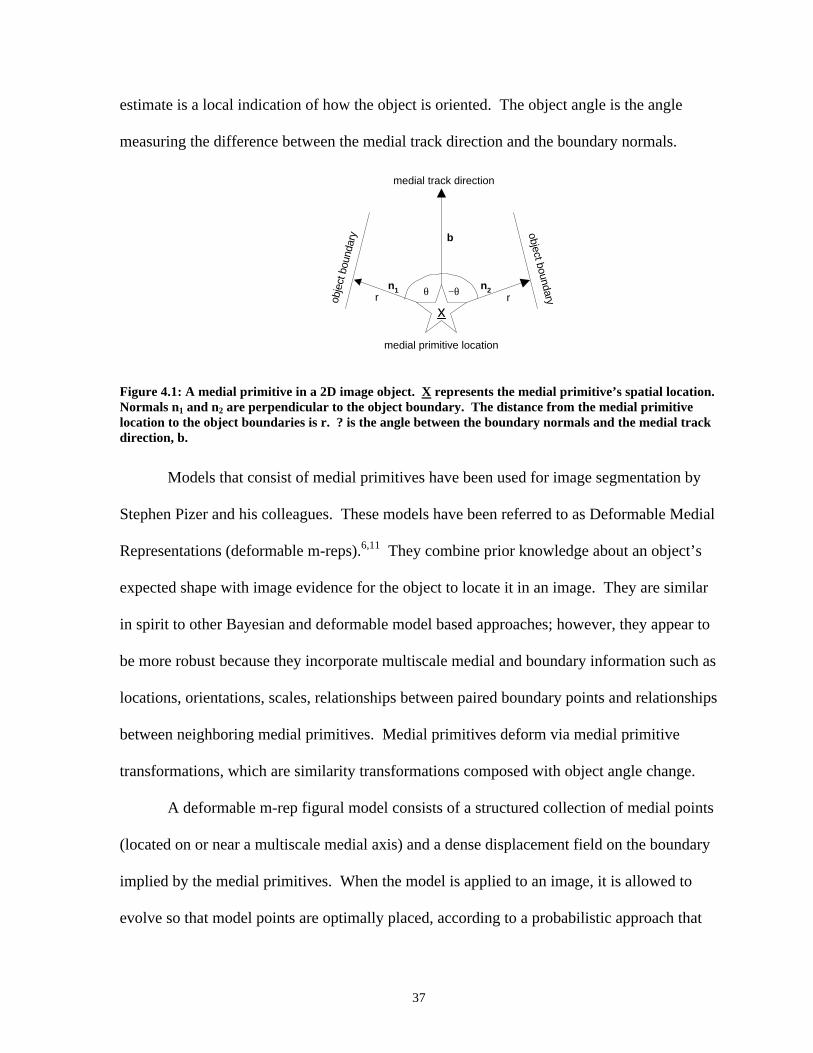
37

estimate is a local indication of how the object is oriented. The object angle is the angle

measuring the difference between the medial track direction and the boundary normals.

xob

ject

bou

ndar

y object boundary

medial primitive location

medial track direction

r rn2n1 θ −θ

b

Figure 4.1: A medial primitive in a 2D image object. X represents the medial primitive’s spatial location. Normals n1 and n2 are perpendicular to the object boundary. The distance from the medial primitive location to the object boundaries is r. ? is the angle between the boundary normals and the medial track direction, b.

Models that consist of medial primitives have been used for image segmentation by

Stephen Pizer and his colleagues. These models have been referred to as Deformable Medial

Representations (deformable m-reps).6,11 They combine prior knowledge about an object’s

expected shape with image evidence for the object to locate it in an image. They are similar

in spirit to other Bayesian and deformable model based approaches; however, they appear to

be more robust because they incorporate multiscale medial and boundary information such as

locations, orientations, scales, relationships between paired boundary points and relationships

between neighboring medial primitives. Medial primitives deform via medial primitive

transformations, which are similarity transformations composed with object angle change.

A deformable m-rep figural model consists of a structured collection of medial points

(located on or near a multiscale medial axis) and a dense displacement field on the boundary

implied by the medial primitives. When the model is applied to an image, it is allowed to

evolve so that model points are optimally placed, according to a probabilistic approach that

38

optimizes the position of the model with respect to the image information (image match),

weighted by the deviation of the overall shape from a model template (geometric typicality).

Deformable m-rep models are created by interactively generating initial medial primitives,

possibly through stimulated multiscale medial axis (core) generation, followed by iterative

refinement of medial primitives. Deformable m-rep models that consist of multiple figures

(that is, they have multiple distinct medial tracks) can be constructed and applied as well. An

example of a deformable M-rep model applied to images from a cardiac nuclear medicine

image sequence is shown in Figure 4.2.

Multiscale deformable m-reps allow a coarse-to-fine approach to image segmentation.

At each scale level, a probabilistic formulation says that a log posterior probability, namely

the log probability of the model given the image information, should be maximized over the

parameters of a geometric transformation appropriate to that scale level. This probability is

found in a Bayesian fashion, by taking the log of a prior of the model M and adding a log

likelihood function of the image information I given the model, and ignoring a term that is

Figure 4.2: The lefthand image is a blood pool frame, two frames after the frame used to create a deformable m-rep model. The middle image shows the deformable m-rep model manually

rotated and translated away (by 4 pixels and 20 degrees) from an optimal position. Following optimization, the deformable m-rep model nicely segments the left ventricle (righthand image).

39

independent of the model’s position and configuration (log(P(I))), as in the following

equation:

)).(log())(log())|(log()|(log( IPMPMIPIMP −+=

The log likelihood function can be defined at each scale level by correlation of the model’s

intensity templates (analytically or statistically defined) with intensity information based on

the implied boundary at the current scale in the image undergoing segmentation.

One example of defining the log priors for the multiscale m-rep segmentation

approach is as follows.9 At the coarsest level of scale, the object level, the log prior is

defined for a candidate similarity transformation as a Gaussian prior on boundary

displacement. At the medial primitive level, the log prior is defined for medial primitive

transformations of the primitive as a Gaussian prior on boundary displacement with a

Markov random field prior relative to the medial primitive transformations of neighboring

medial primitives at this level. At the boundary level of scale, the prior is a Markov random

field prior on the boundary displacement field relative to the displacements of neighboring

boundary points at this level.

Recently, alternatives for defining log priors (geometric typicality) for multiscale

deformable m-rep models have emerged based on the work of Fletcher et al.12 These are

based on the fact, used advantageously by Fletcher et al., that medial primitives are elements

of a Lie group. Based on this property, a distance metric has been defined allowing

comparison of two medial primitives along Lie group geodesics. The distance metric could

be used to measure geometric typicality of a candidate m-rep versus a template m-rep.

Furthermore, the Lie algebra allows definition of “principal geodesic analysis” on members

of a m-rep group. Candidate m-reps could be projected onto principal geodesics and squared

40

differences of projection coefficients between a candidate and a template summed to measure

geometric typicality. Finally, Fletcher et al. have defined Gaussian distributions on m-rep

Lie groups, allowing the definition of Gaussian priors for m-reps.

Deformable m-reps can be used to track the shape changes of an object in an image

sequence, as was shown in Clary et al.13 The final configuration of the deformable m-rep in

a frame is used as the initial configuration in the immediately subsequent frame. Extensions

to the deformable m-rep approach are introduced and evaluated in this work. Features based

on the attributes of special medial primitives known as anchor primitives are used as inputs

to a statistical classifier in order to perform image sequence classification.

Multiscale medial primitives include a width attribute. The width attribute is a local

estimate of object size and is also commonly referred to as the object’s radius. In the case of

medial primitives that are found at the end of medial tracks, that is, “endpoints,” the radius is

a local estimate of the radius of curvature of the boundary. The width attributes of anchor

primitives (detailed in Chapter 5), normalized by their maximum over an image sequence,

are in this work proposed and evaluated as features for classification for both the left

ventricular regional wall motion application and the computer lipreading problem. In

addition, the inter-frame change in the width attribute is used as a feature as well.

Because multiscale deformable m-rep models can robustly track the location of an

object’s middle, data specific to the object middle or near middle can be used as features as

well, if desired. For example, a Gaussian weighted intensity value or intensity profile values

taken near a medial point that corresponds to the middle of the mouth opening may be (a)

useful feature(s) for classification in the lipreading problem. This is due to the fact that, for

some speech, the visibility of the teeth and tongue is an important cue for human

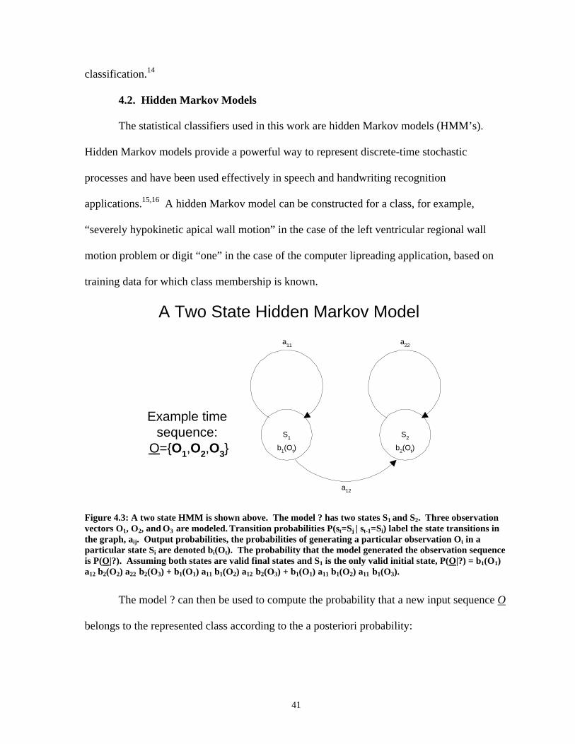
41

classification.14

4.2. Hidden Markov Models

The statistical classifiers used in this work are hidden Markov models (HMM’s).

Hidden Markov models provide a powerful way to represent discrete-time stochastic

processes and have been used effectively in speech and handwriting recognition

applications.15,16 A hidden Markov model can be constructed for a class, for example,

“severely hypokinetic apical wall motion” in the case of the left ventricular regional wall

motion problem or digit “one” in the case of the computer lipreading application, based on

training data for which class membership is known.

S1 S2

a12

a11 a22

A Two State Hidden Markov Model

Example timesequence:

O={O1,O2,O3} b1(Ot) b2(Ot)

Figure 4.3: A two state HMM is shown above. The model ? has two states S1 and S2. Three observation vectors O1, O2, and O3 are modeled. Transition probabilities P(st=Sj | st-1=Si) label the state transitions in the graph, aij. Output probabilities, the probabilities of generating a particular observation Ot in a particular state Si are denoted bi(Ot). The probability that the model generated the observation sequence is P(O|?). Assuming both states are valid final states and S1 is the only valid initial state, P(O|?) = b1(O1) a12 b2(O2) a22 b2(O3) + b1(O1) a11 b1(O2) a12 b2(O3) + b1(O1) a11 b1(O2) a11 b1(O3).

The model ? can then be used to compute the probability that a new input sequence O

belongs to the represented class according to the a posteriori probability:

42

)()()|(

)|(OP

POPOP

λλλ = .

To perform classification, the class assigned to an input sequence is that represented

by the model with the highest probability P(?|O). The prior probability of a particular model

is assumed to be uniformly distributed in this work. The prior probability of an input

sequence is independent of the models and can be ignored. Thus the model ? that maximizes

P(O| ?) is sought across all models. A hidden Markov model is graphically represented in

Figure 4.3 and an example of computing P(O| ?) is given.

A hidden Markov model consists of two components, a finite-state Markov chain and

a finite set of output probability density functions. Models are viewed as “generative,” that

is, the probability that a given model produced a given input sequence is computed. HMM’s

are called “hidden” because the state sequence which generates a particular observation

sequence is not directly observable. In general, either states or transitions in the Markov

chain may have output probability density functions associated with them. In this work, the

output probability densities are associated with the states.

The output probability densities can be used to compute the probability that a

particular state or transition generated a given “observation,” that is, input feature vector. In

the case of continuous parameter HMM’s, observations can be real-valued feature vectors.

Figure 4.3 illustrates a two state first order hidden Markov model that can generate three real-

valued feature vectors (in this example), O1, O2, and O3. aij is the probability of a transition

between states i and j, and p(Ot| Si) is the probability that feature vector at time t was

generated in state Si, bi(Ot). This example under the given assumptions, then, says that the

probability of the model generating the observation sequence O1, O2, and O3 is equal to the

probability of generating the feature vectors via all valid state sequences. The probability of

43

a feature vector given a state is often obtained in hidden Markov model applications from a

Gaussian distribution or a mixture of Gaussian distributions. Maximum likelihood (ML)

estimates of Gaussian distribution parameters can be made to estimate output probability

distribution parameters (and the ML estimates correspond to the usual definitions of

Gaussian model parameters). Maximum likelihood estimation assumes that the training

observations are independent.

Both the parameters of the output probability distributions and the state transition

probabilities for a set of models can be obtained using standard training algorithms, such as

the Baum-Welch re-estimation algorithm, and pre-classified data.17 Once a set of models is

in place, new inputs can be classified using a “decoding” algorithm known as the Viterbi

algorithm, which is based on dynamic programming and gives the value of P(O| ?) for each

model.18

4.3. Summary

Approaches to deformable model based segmentation have included landmark based

methods, boundary based methods, atlas based methods and medial methods. Medial

methods have shown particular promise because of their ability to establish an object-centric

coordinate system that allows correspondence between model points across image object

instances to be defined. Such correspondence is necessary for statistical feature extraction

and is one of the motivating aspects contributing to the definition of anchor primitives in this

work. The anchor primitive based segmentation framework introduced in this work is similar

to landmark based approaches, but it uses symmetries in an m-rep inspired way to reduce the

number of parameters required to represent an image object.

Hidden Markov models are widely used in a number of time sequence classification

44

applications. Features based on anchor primitives are used as inputs to hidden Markov

model based classifiers in this work to classify image sequences. Chapter 5 defines anchor

primitives and discusses specific example models for left ventricles and lips in 2D images.

45

1. T. McInerney and D. Terzopoulos, “Deformable Models in Medical Image

Analysis: A Survey,” Medical Image Analysis, Vol. 1, No. 2, 1996, pp. 91-108. 2. H. Wechsler, Computational Vision, San Diego, CA: Academic Press, Inc., 1990,

p. 369. 3. F.L. Bookstein, “Linear Methods for Nonlinear Maps: Procrustes Fits, Thin-Plate

Splines, and the Biometric Analysis of Shape Variability,” in Brain Warping, A.W. Toga, ed., San Diego: Academic Press, 1999.

4. S. Joshi and M.I. Miller, "Landmark Matching Via Large Deformation

Diffeomorphisms," IEEE Transactions on Image Processing, Vol. 9, No. 8, Aug. 2000, pp. 1357-1370.

5. G.E. Christensen, S.C. Joshi, and M.I. Miller, “Volumetric Transformation of

Brain Anatomy,” IEEE Transactions on Medical Imaging, Vol. 16, No. 6, Dec. 1997. 6. M. Hébert, H. Delingette, and K. Ikeuchi. Shape representation and image

segmentation using deformable surfaces. IEEE Transactions on Pattern Analysis and Machine Intelligence, Vol. 17, No. 7, June 1995.

7. G. Szekely, A. Kelemen, Ch. Brechbuehler and G. Gerig, “Segmentation of 3D

objects from MRI volume data using constrained elastic deformations of flexible Fourier surface models,” Medical Image Analysis (MEDIA), Vol. 1, No. 1, March 1996, pp. 19-34.

8. S.M. Pizer, D.S. Fritsch, P. Yushkevich, V. Johnson, and E. Chaney,

“Segmentation, Registration, and Measurement of Shape Variation via Image Object Shape,” IEEE Transactions on Medical Imaging, Vol. 18, No. 10, pp. 851-865.

9. S.M. Pizer, S. Joshi, P.T. Fletcher, M. Styner, G. Tracton, and J.Z. Chen,

“Segmentation of Single-Figure Objects by Deformable M-reps,” MICCAI 2001, W.J. Niessen and M.A. Viergever, eds., Lecture Notes in Computer Science, Vol. 2208, pp. 862-871.

10. S. Joshi, S.M. Pizer, P.T. Fletcher, P. Yushkevich, A. Thall, and J.S. Marron,

“Multiscale Deformable Model Segmentation and Statistical Shape Analysis Using Medial Descriptions,” IEEE Transactions on Medical Imaging, Vol. 21, No. 5, May 2002.

11. D.S. Fritsch, S.M. Pizer, L. Yu, V. Johnson, and E.L. Chaney, “Localization

and Segmentation of Medical Image objects using Deformable Shape Loci,” Information Processing in Medical Imaging 1997, Lecture Notes in Computer Science, Vol. 1230, pp. 127-140.

46

12. P.T. Fletcher, S. Joshi, C. Lu and S.M. Pizer, “Gaussian Distributions on Lie

Groups and Their Application to Statistical Shape Analysis,” Submitted to IPMI, 2003. 13. G.J. Clary, S.M. Pizer, D.S. Fritsch, and J.R. Perry, “Left Ventricular Wall

Motion Tracking via Deformable Shape Loci,” in Computer Assisted Radiology and Surgery, Proceedings of the 11th International Symposium and Exhibition, H.U. Lemke, M.W. Vannier, and K. Inamura, eds., Amsterdam: Elsevier Science B.V., 1997, pp. 271-276.

14. M. McGrath, A.Q. Summerfield, and N.M. Brooke, “Roles of lips and teeth in

lipreading vowels,” Proceedings of the Institute of Acoustics, Vol. 6, No. 4, pp. 401-408. 15. F. Jelinek, “Continuous speech recognition by statistical methods,” Proceedings

of the IEEE, Vol. 64, 1976, pp. 532-556. 16. K. S. Nathan, H. S. M. Beigi, J. Subrahmonia, G. J. Clary, and H. Maruyama,

"Real-Time On-Line Unconstrained Handwriting Recognition Using Statistical Methods," Proceedings of IEEE International Conference on Acoustics, Speech, and Signal Processing, 1995.

17. X.D. Huang, Y. Ariki, and M.A. Jack, Hidden Markov Models for Speech

Recognition, Edinburgh: Edinburgh University Press, 1990. 18. A.J. Viterbi, “Error bounds for convolutional codes and an asymptotically

optimum decoding algorithm,” IEEE Transactions on Information Theory, Vol. 13, 1967, pp. 260-269.

Chapter 5

Image Sequence Classification via Anchor Primitives

In this chapter, details of the approach to classifying image sequences using anchor

primitives are given. A general discussion of anchor primitives is followed by sections on

applying anchor primitives to heart image sequences and lip image sequences.

5.1. Correspondence and Deformable Models A problem with the deformable m-reps approach (and with other deformable model

based approaches) has been referred to as the correspondence problem.1 The correspondence

problem is that model points may not be consistently placed (with respect to salient image

features) by the optimization algorithm on different instances of an image object, because of

the sparse nature of the models. For example, medial points may slide toward one end of a

figure or the other along the medial track. Reliable measurements for statistical feature

extraction cannot be made unless model points are consistently placed.

One approach to enforcing correspondence is to penalize heavily for any sliding in

the medial track direction, assuming a reasonable initial model point. The problem is, what

does “heavily” mean? Another approach is to consider endpoints to exhibit correspondence,

and to sample uniformly between the two endpoints of a figure. The problem is that

48

endpoints exhibit sliding behavior as well (as illustrated in Figure 5.1), so considering them

to exhibit correspondence is dangerous.

Figure 5.1: Medial primitives, including end primitives, may “slide,” that is, change scale and location between frames of an image sequence, not because they are following a corresponding image object feature but because they begin to track a different image feature.

The approach taken here to combating the correspondence problem is to define and

use special primitives for image segmentation based on medial primitives. I begin by

defining correspondence more precisely. Primitives placed on multiple instances of an image

object are said to have correspondence if their attributes are consistent relative to some

repeated property of the image object, e.g., a salient image feature. My corresponding

primitives are called anchor primitives, which are placed using image measurements in

various parts of an image and prior knowledge of the expected geometric relationships

between the locations for the image measurements. To place anchor primitives, an objective

function is optimized that combines image measurements and geometric penalty terms that

incorporate the prior knowledge. To place deformable m-reps that include anchor primitives,

penalty terms that capture the expected relationships between attributes of the anchor

Object Boundary

End Primitive Location

49

primitives and between anchor primitives and other primitives are also included in the

objective function.

5.2. Anchor Primitive Definition

The central idea behind anchor primitives is that if the object is a closed object, it is

possible to keep the object’s model simple, in terms of the number of primitives. A single

anchor primitive may be used to represent a closed object. The “center point” may be found

by dividing the boundary into two pieces twice (e.g., a left and right piece and a top and

bottom piece) and measuring boundariness along each piece. Note that the pieces may

overlap—i.e., the left piece may share a portion of the top piece and a portion of the bottom

piece, etc. Each of the boundary pieces may be represented by arbitrarily complex curves,

but complexity is limited in practice by the increase in the size of the search space. The use

of anchor primitives simplifies deformable m-reps in terms of the number of primitives

required, but due to complex boundary representations the anchor primitives themselves may

be more complex than previously defined medial primitives. The locations for the anchor

primitive image measurements are chosen based on the expected locations of corresponding

geometric entities in the image.

The purpose of anchor primitives is to provide a stable framework for consistent and

concise statistical feature definition. Anchor primitives consist of the following:

• A center point location. Note that for a closed 2D object, a “center point” can

be defined by dividing the object boundary into pieces and specifying

symmetric relationships between the boundary pieces along the medial axis

(or axes). Equivalently, a closed 2D object can be blurred until its primary

medial axes emerge. The “center point” is typically medial at more than one

50

scale and in more than one medial track direction simultaneously. The anchor

primitive center point location provides a reference point for defining salient

image object feature locations and distances that are also attributes of the

anchor primitive model.

• Salient image object feature locations. Image object feature locations define

the locations of geometric entities including those boundary pieces

represented by parametric curves or deformable m-rep models. For example,

salient image object feature locations along the left ventricular wall are chosen

by the model builder (the author in this example) in the left ventricle’s anchor

primitive model--septal wall center, basal wall center, apical wall center, and

lateral wall center. Salient image object feature locations along the lips are

chosen in the lip anchor primitive model--upper left lip and lower left lip

corner, upper lip center, upper right lip and lower right lip corner.

• Curve parameters or deformable m-rep model parameters. Anchor primitives

represent geometric entities of the image object using parametric curves or

deformable m-rep models. The parametric curves or deformable m-rep

models can be arbitrarily complex. The salient image object feature

(geometric entity) locations may specify curve parameters or locations of

medial nodes. Parametric curves or deformable m-rep models constrain the

search space during anchor primitive fitting and define geometric models for

model to image match measurement making.

• Constraints on the relationships between image object feature locations.

Constraints may be hard or soft. A hard constraint specifies a fixed

51

relationship between two geometric entities. A soft constraint penalizes

model configurations that vary from the typical geometry of the entities.

Consider the top view of a salamander in motion captured by an image sequence. A

schematic of such a salamander is pictured in Figure 5.2 along with its anchor primitive.

Such an image sequence could be used to study the gait of the salamander.

(X, Y)

1

4

2

35

6

Figure 5.2: A schematic of a salamander and its anchor primitive model. The stars represent salient image object feature locations (geometric entity locations).

52

Consider the attributes of the salamander anchor primitive pictured in Figure 5.2:

• A center point location denoted by (X, Y). The salamander has a center that is

medial with respect to both the tip of its nose and the tip of its tail and the left

and right sides of its body.

• Salient image object feature locations denoted by (1,2,3,4,5,6). There are six

locations corresponding to salient image object features: head, tail, left front

leg, right front leg, left hind leg, right hind leg. Locations may be specified in

the most convenient coordinate system. Locations may consist of end points

of boundary pieces or medial tracks rather than single locations.

• Curve parameters. Supplemental parameters that specify control points or

curvatures may be used to specify curves representing the salamander’s salient

geometric entity boundaries. Such control points could be at the tips of the

legs, head and tail, for example. Alternatively, another parametric

representation such as a Fourier representation could be used for the salient

image object features (geometric entities).

• Constraints on the relationships between image object feature locations.

There are hard constraints on distances between adjacent legs on opposite

sides of the body (between “front legs” or “hind legs”) because the body is

considered to be rigid in cross-section by this example model. There are soft

constraints on distances between legs on the same side of the body (between

“right legs” or “left legs”) because the body is limited in the amount it can

turn between frames of an image sequence, assuming an appropriate frame

rate.

53

The anchor primitive attributes include the center location and the salient geometric

entity model definitions. The (X,Y) location of the center point is the (X, Y) attribute of an

anchor primitive. The remaining anchor primitive attributes are parameters used to define

curves or deformable m-rep models representing salient geometric entities of the object.

Such attributes may include angles, scales, and explicit locations relative to the center point.

In addition, constraints on the placement of and properties of the geometric entities and their

relationships to one another play an important role in anchor primitive placement. By fitting

models of the most important geometric entities of an object to local image data and

constraining their placement relative to one another, anchor primitives are placed in an image

and globally represent a closed image object.

Consistently placing anchor primitives on image objects from a population allows

statistical models of the population to be efficiently trained and to exhibit discriminatory

power. Anchor primitives are consistently placed because they utilize local image object

features corresponding to salient geometric entities in a globally optimal model placement

approach. By virtue of anchor primitives having long curve sequences to represent salient

geometric entities, and making image measurements only on salient geometric entities where

intensity variance is limited, the anchor primitive maintains correspondence more effectively

than many alternative geometric models. Thus, variance of statistical features defined by

anchor primitives due to model placement is significantly reduced.

5.3. Anchor Primitive Representing the Left Ventricle

For example, in the left ventricular wall motion tracking application (using MLAO

view ventriculograms), there is a point that is medial with respect to the left and right (i.e.,

54

septal and lateral) boundaries of the left ventricle (LV) and also medial with respect to the

top and bottom (i.e., basal and apical) boundaries of the ventricle.

Figure 5.3: The anchor primitive for left ventricular segmentation consists of a location, two different scales (the distances between the center location and each set of paired boundaries), two orientations (the directions of the rays along which the scales are measured) and four curvature values. Each boundary piece is approximated by a partial ellipse. The a values are curvature parameters of the partial ellipses.

The location of the anchor primitive is defined to be the point that serves as the basis

for measurement making where the objective function that combines model to image match

and geometric typicality is optimal. For example, the point that is medial with respect to the

septal and lateral and basal and apical boundaries is the anchor primitive location in the left

ventricular wall motion tracking application. Included in the LV anchor primitive (see

Figure 5.3) are two scales, s1 and s2, which are the distances between the anchor primitive

location and the boundaries. s1 corresponds to the distance to the septal and lateral

boundaries and s2 to the basal and apical boundaries. Also included in the primitive are two

orientation parameters, ?1 and ?2, which are the directions with respect to the horizontal of

the lateral and basal boundaries, respectively. α1, α2, α3, and α4 are parameters of four

Anchor Primitive for LV Segmentation

η1

η2 s1

s1

s2

s2

x, y

α1

α4

α3

α2

A={x, y, s1, s2, η1, η2, α1, α2, α3, α4}

55

independent ellipses (see Figure 5.4) that model the boundaries in the ?1, ?2, π+?1 and π+?2

directions, respectively. Each of these ellipses is used to define a kernel with partial elliptical

level sets that is used to measure boundariness according to the primitive parameters.

Partial ellipses are chosen to model the boundary pieces because of their relative

simplicity. The anchor primitive parameters are used to render each ellipse in a bitmap. The

Danielson Distance Transform is used to compute the distance from each pixel in the bitmap

to the rendered ellipse. These distances are then used as the radii for a derivative of a

Gaussian in polar form to compute the kernel values. More general curves could be chosen

that might make anchor primitives more powerful, including splines, curves generated using

Fourier descriptors and hodograph curves.

u

v

s

αs

u2 + v2 /α2 = s2

u2 + v2 /α12 = s1

2 /α12

Figure 5.4: The anchor primitive α values, the ratios of partial ellipse axis lengths, are defined as in this figure. The u and v coordinate axes lie along the axes of the ellipse. s and αs are the lengths of the axes of the ellipse. The second equation above shows the relationship between α1 and s1, for example, in the defined anchor primitive of Figure 3. The second equation above is obtained by letting s1=α1*s.

56

Anchor primitives make it possible to make an object measurement that is consistent

with the expected behavior of the object over an image sequence. Figure 5.5 shows how a

length measurement of the left ventricle changes as a function of time. The measured length

is the distance between the anchor primitive location and the location of the boundariness

measurement in the direction of the apex. As is shown, the length gets smaller as the heart

contracts and becomes larger again as the ventricle expands. The length changes are

consistent with the expected behavior of the left ventricle in a ventriculogram.

Figure 5.5: The distance S2 between the anchor primitive location and the apex decreases as the

heart contracts and then increases as the heart expands. 5.4. Approach to Fitting Anchor Primitives to the Left Ventricle

The approach to image sequence classification is to find optimal anchor primitives for

each frame of the sequence and then use geometric features based on the anchor primitives

0 5 10 15 20 25 30 35 6.5

7

7.5

8

8.5

9

9.5

10 S2 Vs. Time

Time (Frame Number)

S2

57

and other anchor primitive implied features across the sequence as the basis for statistical

classification. Anchor primitive segmentation of each frame in the sequence proceeds as

follows. Parameters of an anchor primitive may be manually initialized for the first frame by

adjusting the size, location and shape of the anchor primitive to visually match the image

object. For each image of the sequence beyond the first frame, the initial parameters of the

anchor primitive are the optimal parameters of the primitive for the previous frame. (Finding

optimal anchor primitive parameters is described below.) Parameters of the template anchor

primitive on which geometric penalty calculations are based are the optimal anchor primitive

parameters for the previous frame as well.

In any given frame, an evolutionary optimization strategy is used to find optimal

parameters for an anchor primitive with respect to the image object to be segmented.

5.4.1. Objective Function

The objective function optimized by the evolutionary strategy consists of the

combination of an image match function and a geometric penalty function. The objective

function tends to have local optima, so a stochastic optimization method such as evolutionary

optimization is useful. When the objective function is evaluated, the image match function

and the penalty function are computed as outlined in the next section.

5.4.2. Image Match Function

The anchor primitive for the left ventricle specifies that boundariness measurements

should be made in four directions specified by two orientation angles. (Two of the four

directions are π radians from the directions specified by the two orientation angles.) The

orientation angles, anchor primitive scales and axis length ratios determine partial ellipses

along which boundariness measurements are made. A weighted sum of the four

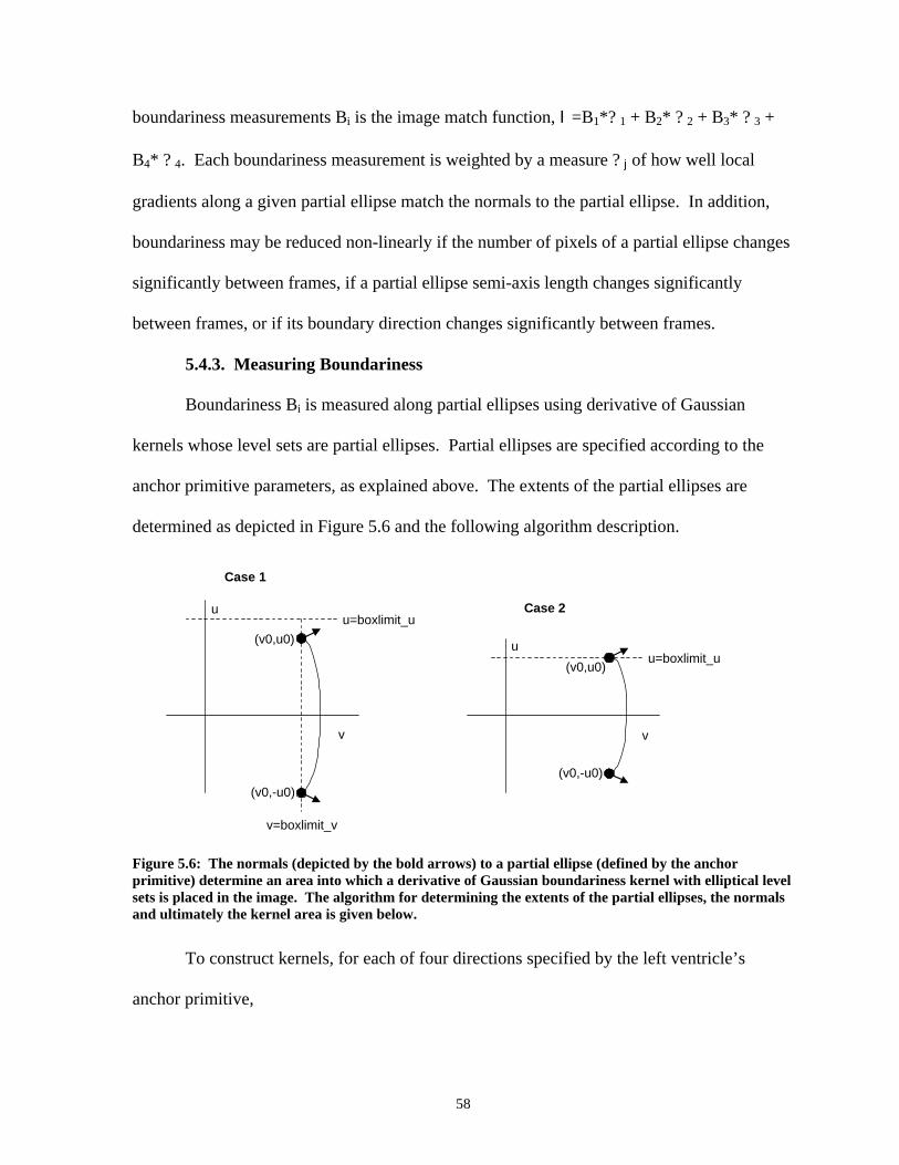
58

boundariness measurements Bi is the image match function, I =B1*? 1 + B2* ? 2 + B3* ? 3 +

B4* ? 4. Each boundariness measurement is weighted by a measure ? j of how well local

gradients along a given partial ellipse match the normals to the partial ellipse. In addition,

boundariness may be reduced non-linearly if the number of pixels of a partial ellipse changes

significantly between frames, if a partial ellipse semi-axis length changes significantly

between frames, or if its boundary direction changes significantly between frames.

5.4.3. Measuring Boundariness

Boundariness Bi is measured along partial ellipses using derivative of Gaussian

kernels whose level sets are partial ellipses. Partial ellipses are specified according to the

anchor primitive parameters, as explained above. The extents of the partial ellipses are

determined as depicted in Figure 5.6 and the following algorithm description.

v

u

u

v

u=boxlimit_u

v=boxlimit_v

u=boxlimit_u

Case 1

Case 2

(v0,u0)

(v0,-u0)(v0,-u0)

(v0,u0)

Figure 5.6: The normals (depicted by the bold arrows) to a partial ellipse (defined by the anchor primitive) determine an area into which a derivative of Gaussian boundariness kernel with elliptical level sets is placed in the image. The algorithm for determining the extents of the partial ellipses, the normals and ultimately the kernel area is given below.

To construct kernels, for each of four directions specified by the left ventricle’s

anchor primitive,

59

− boxlimit_v = Beta * r (r is semi-axis length for current partial ellipse axis along the current direction – r and “current direction” are anchor primitive parameters. Beta is a hyperparameter.)

− boxlimit_u = Beta * os (os is semi-axis length for ellipse corresponding to the other direction.)

− find intersection of ellipse with line v = boxlimit_v, call it (v0, u0) (Case 1 of Figure 5.6)

− if (u0 > boxlimit_u) (then apply Case 2 of Figure 5.6) − u0 = boxlimit_u − v0 comes from intersection of ellipse and line u = boxlimit_u

− Compute normals to ellipse at (v0, u0) and (v0, -u0) − If point (v,u) falls within area between normals and is less than 3*sigma (sigma =

ρ*r) from the ellipse then the kernel is non-zero at (v,u). Each kernel value is computed as a derivative of a Gaussian with standard deviation sigma along a line perpendicular to the partial ellipse.

The image data is convolved with such a kernel to get a boundariness value for each

of the four partial ellipses specified by the anchor primitive parameters.

5.4.4. Geometric Penalty Function for Left Ventricle Anchor Primitive

A penalty is imposed when the direction of the left-most boundary point as defined by

the anchor primitive differs from the direction of the center of the boundary of the left partial

ellipse. A similar penalty is imposed when the direction of the southern-most boundary point

as defined by the anchor primitive differs from the direction of the center of the boundary of

the bottom partial ellipse. Another term penalizes variation in the difference between the two

orientation parameters from π/2. These model configuration penalties reflect prior

knowledge that the position of the left ventricle is largely consistent between frames and

across patients.

Most geometric penalty function terms penalize changes in the anchor primitives

between the current frame and the previous frame. The more change in any anchor primitive

value from frame-to-frame, the stiffer the penalty. This reflects prior knowledge of the

60

physics of the contraction and expansion of the left ventricle; only limited motion is possible

between frames of the image sequence.

5.5. Anchor Primitive Based Segmentation of Lip Image Sequences

To segment the lip image sequences, anchor primitives are placed in each frame by

optimizing an objective function composed of image match terms and geometric penalty

terms. Image measurements are made at places that have correspondence between different

frames—different frames across time and across speakers. Corresponding places are three

boundary segments: the left edge of the upper lip boundary, the right edge of the upper lip

boundary and the lower lip boundary. The shape of each of the three boundary segments is

modeled by a quadratic of the form:

222 222)( scsbsasbsaasf +−++−=

a

b

c

where a, b, and c are control points. For each of the boundary segments, a and c

correspond to the end points of the segments. b does not necessarily lie on the curve; it is

similar to a B-spline control point. A quadratic was chosen because it is simple to

compute and it models the boundary segment shapes well.

The anchor primitive model used to segment lip images is pictured below.

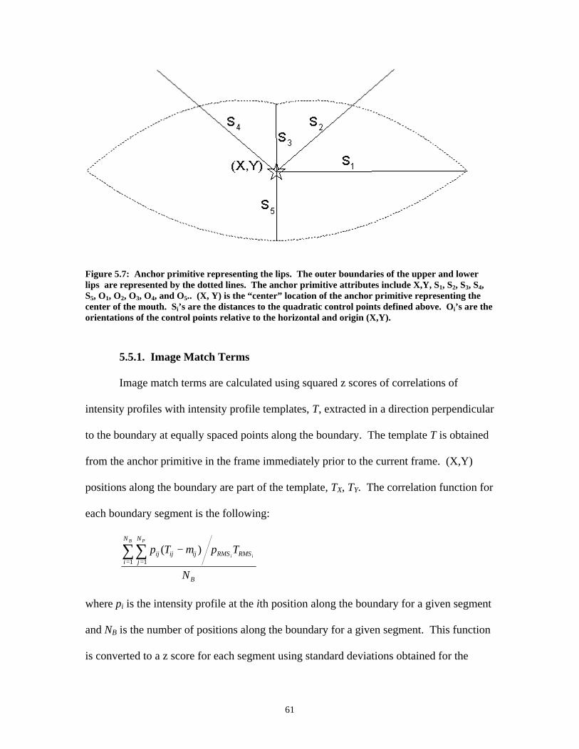
61

Figure 5.7: Anchor primitive representing the lips. The outer boundaries of the upper and lower lips are represented by the dotted lines. The anchor primitive attributes include X,Y, S1, S2, S3, S4, S5, O1, O2, O3, O4, and O5.. (X, Y) is the “center” location of the anchor primitive representing the center of the mouth. Si’s are the distances to the quadratic control points defined above. Oi’s are the orientations of the control points relative to the horizontal and origin (X,Y).

5.5.1. Image Match Terms

Image match terms are calculated using squared z scores of correlations of

intensity profiles with intensity profile templates, T, extracted in a direction perpendicular

to the boundary at equally spaced points along the boundary. The template T is obtained

from the anchor primitive in the frame immediately prior to the current frame. (X,Y)

positions along the boundary are part of the template, TX, TY. The correlation function for

each boundary segment is the following:

B

N

iRMSRMSij

N

jijij

N

TpTpB

ii

P

∑∑= =

−1 1

)( µ

where pi is the intensity profile at the ith position along the boundary for a given segment

and NB is the number of positions along the boundary for a given segment. This function

is converted to a z score for each segment using standard deviations obtained for the

62

correlation values from training sequences. The means for the z scores are taken to be

the maximum possible correlation value for each boundary segment. Thus, the more a

correlation value is below the maximum possible value, the worse (larger) the z score.

The squared z score is the image match term for a given boundary segment.

5.5.2. Geometric Penalty Terms

A geometric penalty reflects that the movement of the mouth is limited between

frames. The penalty measures the consistency of the shape of the mouth in the current

frame with the previous frame and ensures that the shape is “lip-like.” The geometric

penalty terms are added to the objective function for each boundary segment. For a

particular boundary segment, the penalty is the following:

BT

N

iYiXi

NS

TYTXB

ii∑=

−+−1

22 )()(

where (X , Y) are positions along the boundary in the current frame, and (TX , TY ) are the

boundary positions of the template (boundary positions in the previous frame). ST is the

scale parameter of the template anchor primitive for this particular boundary segment.

Geometric penalties are converted to squared z scores for combining with the image

match terms in the objective function. Conjugate gradient optimization minimizes

accumulated squared z scores to find optimal anchor primitive parameters.

The following chapter discusses the results of classifying image sequences when

the anchor primitive based segmentation method is combined with a statistical classifier.

5.5.3. Tracking Approach for Lip Image Sequences

In the experiments reported in the next chapter, the first and last frames of the lip

image sequences are segmented manually. The manual segmentations are used to

63

initialize the tracking process for both forward in time and backwards in time tracking.

Templates, including intensity profiles and boundary positions, are defined for the first

and last frames using the manual segmentations, and templates are defined for the

remaining frames by the optimal model position in each frame. Templates are used in

immediately subsequent frames to compute model to image match and geometric

typicality in either the forward or backwards in time directions.

The algorithm for picking the best segmentation of each frame is the following for

the considered digit classification problem. Start from the beginning of the sequence.

For each frame, if the score corresponding to forward in time tracking is better, choose

the model configuration for forward in time tracking. If the score corresponding to

backwards in time tracking is better, choose the model configuration for backwards in

time tracking for all of the remaining frames. In other words, once the switch is made to

the model configuration for backwards in time tracking, never switch back to the forward

in time model configurations. The motivation for this algorithm is in tracking a digit like

“four,” the lower lip dramatically accelerates when the voiceless plosive /ph/ is released

and the image sequence capture process undersamples the motion in the studied data set.

Forward tracking correctly tracks lip motion up to the time of the release. Backwards

tracking correctly tracks lip motion from the end of the sequence to the frame

immediately following the release. This approach only allows for one dramatic

acceleration per word. Detecting these discontinuity events is a subject for future

research.

64

5.6. Classification of Image Sequences Using Anchor Primitives

Anchor primitives have been applied to statistical feature extraction for image

sequence classification to show that they provide concise and consistent statistical

features. For both the left ventricular wall motion classification problem and the

computer lipreading problem, anchor primitive attributes and functions of anchor

primitive attributes are selected in each frame of each image sequence to form a time

sequence of feature vectors. The time sequences of feature vectors are used for hidden

Markov model based classification of the image sequences. The features selected for

statistical classification, classification results and conclusions about anchor primitives are

detailed in the following chapter.

65

1. S.M. Pizer, D.S. Fritsch, P. Yushkevich, V. Johnson, and E. Chaney,

“Segmentation, Registration, and Measurement of Shape Variation via Image Object Shape.” IEEE Transactions on Medical Imaging, Vol. 18, No. 10, pp. 851-865.

Chapter 6

Results and Conclusions

“An interesting early application of setting the optimal criterion is seen in Pascal’s famous “wager.” In 1670, Blaise Pascal, a French mathematician, claimed that to believe in God was rational. He noted that there are two possibilities, existence of God or nonexistence of God, and two possible responses, belief in God or disbelief in God. Pascal argued that, even if the probability of God’s existence is extremely small, the gain (value) of asserting His existence and the cost of denying it make belief in God the rational choice. In [Theory of Signal Detection] terms, the decision criterion should be set infinitely low because the value of a hit is infinitely high as is the cost of a miss, and at the same time there is no cost to a false alarm and no value to a correct rejection. Thus, `If you gain, you gain all; if you lose, you lose nothing. Wager, then, without hesitation that He is’ (Pensee No. 233, Pascal, 1958).” --from Psychophysics: The Fundamentals, pp. 112-113.

To evaluate the performance of the anchor primitive based image sequence

classification methodology, classification experiments were designed that used attributes of

anchor primitives as features. For each of the two driving problems of this dissertation, left

ventricular wall motion classification and computer lipreading, several aspects will be

discussed in this chapter. They include the following:

• a brief review of the motivation and background for the classification

application,

• the anchor primitive model used to represent the image objects,

• a summary of possible features for statistical classification implied by the

anchor primitives,

• the database used for classification experiments,

67

• results of semi-automatically segmenting the image objects through the image

sequences,

• the assumptions made about sequence segmentation when performing

classification experiments,

• properties of the statistical classifiers used for classification experiments,

• the approach to feature selection from the population of features implied by

the anchor primitives, and

• results of this work compared to other classification results. Bases for

comparison include automatic classification results of other researchers on the

same task in the case of the lipreading results and results of human expert

observers in the case of the left ventricular wall motion task.

The chapter finishes with conclusions that can be drawn from the results and

summarizes how the results support the contributions of the work outlined in Chapter 1.

6.1. Left Ventricular Regional Wall Motion Analysis

As was stated in Chapter 2, analysis of the motion of the left ventricle’s walls can be

performed using blood pool image sequences to aid in the diagnosis of coronary artery

disease and determine the impact of chemotherapy on the heart muscle. Human experts

watch “movie loops” (thirty-two frame image sequences) of the left ventricle’s blood pool.

The volume of the blood pool decreases and increases as the left ventricle contracts and

expands. What this means in image terms is that the area of the bright spot representing the

left ventricle decreases and increases over time. Human experts watch for irregularities of

motion of the regions of the left ventricle. If a region moves irregularly, the coronary artery

supplying blood to it may be blocked or partially blocked or the muscle tissue may be

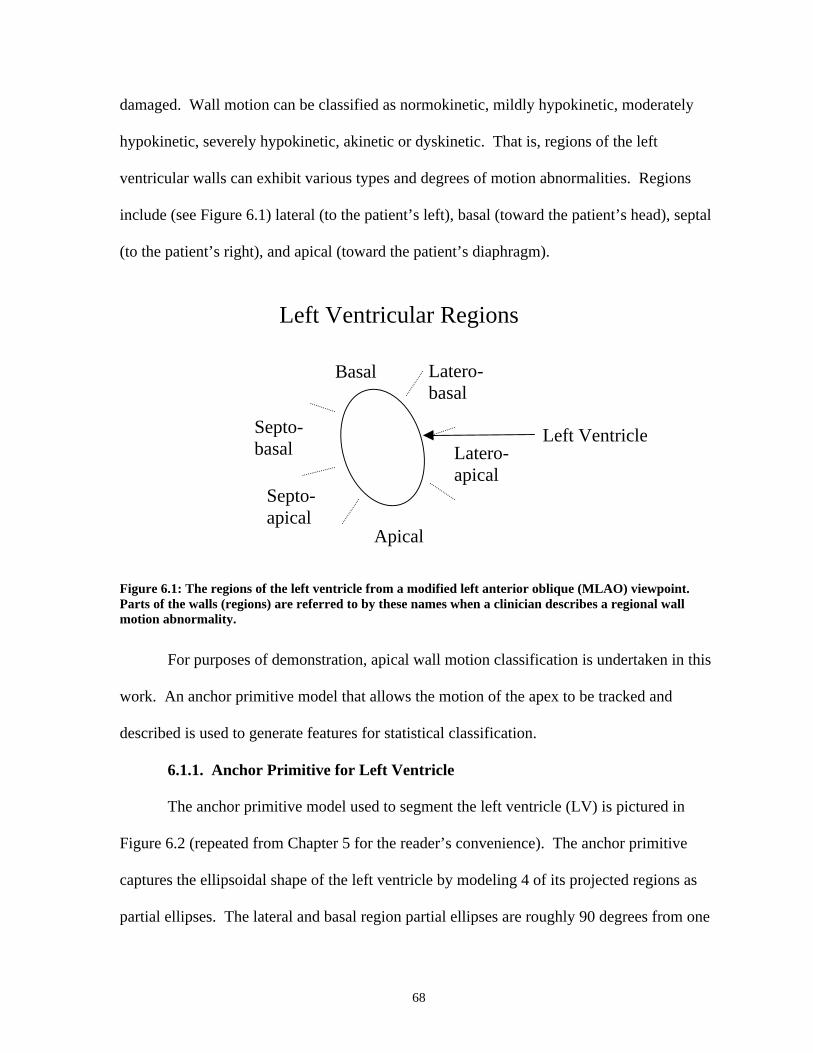
68

damaged. Wall motion can be classified as normokinetic, mildly hypokinetic, moderately

hypokinetic, severely hypokinetic, akinetic or dyskinetic. That is, regions of the left

ventricular walls can exhibit various types and degrees of motion abnormalities. Regions

include (see Figure 6.1) lateral (to the patient’s left), basal (toward the patient’s head), septal

(to the patient’s right), and apical (toward the patient’s diaphragm).

Figure 6.1: The regions of the left ventricle from a modified left anterior oblique (MLAO) viewpoint. Parts of the walls (regions) are referred to by these names when a clinician describes a regional wall motion abnormality.

For purposes of demonstration, apical wall motion classification is undertaken in this

work. An anchor primitive model that allows the motion of the apex to be tracked and

described is used to generate features for statistical classification.

6.1.1. Anchor Primitive for Left Ventricle

The anchor primitive model used to segment the left ventricle (LV) is pictured in

Figure 6.2 (repeated from Chapter 5 for the reader’s convenience). The anchor primitive

captures the ellipsoidal shape of the left ventricle by modeling 4 of its projected regions as

partial ellipses. The lateral and basal region partial ellipses are roughly 90 degrees from one

Left Ventricle

Basal

Apical

Septo- apical

Latero- apical

Latero- basal

Septo- basal

Left Ventricular Regions

69

another. The septal and apical partial ellipses are 180 degrees from the lateral and basal

partial ellipses, respectively. The nature of the partial ellipse based anchor primitive is

detailed in Chapter 5.

Figure 6.2: The anchor primitive for left ventricular segmentation consists of a location, two different scales (the distances between the center location and the boundaries), two orientations (the directions of the rays along which the scales are measured) and four curvature values. Each boundary piece is approximated by a partial ellipse. The a values are curvature parameters of the partial ellipses. The length of each partial ellipse is determined by its a and scale values according to an algorithm given in Chapter 5.

Attributes of the anchor primitive model are given in the Figure 6.2 and are used as a

basis for defining statistical features for left ventricular apical motion classification. The

attributes include an (x,y) anchor primitive location, distances from the anchor primitive

location to the lateral and septal and basal and apical regions, respectively, orientations

relative to the horizontal of the lateral and basal regions (the septal and apical regions are 180

degrees from the lateral and basal regions, respectively) and curvature parameters of each

region’s partial ellipse.

Anchor Primitive for LV Segmentation

η1

η2 s1

s1

s2

s2

x, y

α1

α4

α3

α2

A={x, y, s1, s2, η1, η2, α1, α2, α3, α4}

70

6.1.2. Left Ventricle’s Statistical Features Implied by the Anchor Primitive Model

With the exception of the anchor primitive position and orientations, I experimented

with each of the attributes of the anchor primitive model as statistical features for

classification. In addition, inter-frame changes in attributes were used as features as well.

Table 6.1 summarizes the left ventricle anchor primitive attributes that were used as features

for statistical classification. Some of these are actual attributes, and others, with names

starting with “d,” are inter-frame differences in the designated attribute. For example, dα3 is

the frame-to-frame change in curvature α3. Position and orientation were not considered

because apical wall motion should be independent of absolute left ventricle position and

rotation. Because the number of anchor primitive attributes is relatively small, it was

possible to evaluate all of the remaining attributes as potential statistical features for

classification, as discussed in the section below on feature selection.

Feature S1 S2 α1 α2 α3 α4 dS1 dS2 dα1 dα2 dα3 dα4

Table 6.1: Attributes of left ventricle anchor primitive model used as features for classification. Names of features correspond to the names given in Figure 6.2. dx is defined as the inter-frame change in attribute x.

6.1.3. Left Ventricular Image Data

Forty ECG gated blood pool equilibrium stress cases were selected for this study by a

single radiologist who specializes in cardiac nuclear medicine. Abnormal wall motion

typically is observed when the patient is subjected to exercise or medicinally induced stress.

Figure 6.3 shows one of the cases. An automatic classifier was designed to distinguish

between normal and abnormal apical motion. “Truth” was defined as a consensus of the

opinions of two human experts on the motion of the apex. The experts’ diagnoses with

respect to the motion of the apex were the same in 28 of the 40 cases. The 28 cases on which

the experts agreed were studied in this work. The remaining 12 cases were discarded. Any

71

abnormalities affecting the septal-apical, apical, or latero-apical regions were considered to

be apical motion abnormalities. The utility of defining a consensus of two experts as “truth”

is given by the following argument.

Figure 6.3: An example ECG gated blood pool equilibrium 32 frame image sequence. The camera is at the MLAO viewpoint, thus the left ventricular chamber is in the lower right portion of each frame. Frame at time 0 is at the upper left corner. Time increases from left-to-right and from top-to-bottom.

72

Assume that a “golden truth” exists for each case. The probability that the experts are

wrong (event “W”—they disagree with golden truth) given they agree (event “A”) should be

as low as possible to justify using a consensus of two experts as truth. Using Bayes’ Rule,

)()()|(

)(AP

WPWAPAWP = .

P(A) can be obtained using a frequency based estimate: 28/40=0.7 is the frequency

based probability of the experts’ agreement. Also,

.)(

),()|(

WPWAP

WAP =

P(A,W) = P(A) – P(A,R), where R is the event that both experts agree with golden

truth.

Also, ),(),(),( RalBothAbnormPRBothNormalPRAP += , where “BothNormal” and

“BothAbnormal” are the events where the experts agreed on the same normal or abnormal

diagnosis. Continuing,

).|()()|()(),( alBothAbnormRPalBothAbnormPBothNormalRPBothNormalPRAP +=

To reflect a lack of information about the relationship between the experts’ agreement

on normality or abnormality and their agreement with golden truth, I use the relationship

P(R|BothNormal)=P(R|BothAbnormal)=P(R|A). Again using Bayes’ Rule,

.)()(

)()()|(

)|(APRP

APRPRAP

ARP ==

P(A|R)=1 by the definitions of event R and event A. Substituting gives the following

equation for P(W|A) (the probability the experts are wrong given that they agree):

73

)(

))()(

)()()(

)(()()|(

APAPRP

alBothAbnormPAPRP

BothNormalPAPAWP

+−= .

Also, the expression above for P(W|A) reduces to the following:

)()()(

)|(AP

RPAPAWP

−= .

This simplification is due to the fact that P(A)=P(BothNormal) + P(BothAbnormal).

Also, this simplification corresponds to the argument made above that P(A|R)=1, so

P(A,R)=P(R).

A plot of P(W|A) versus P(R) for the estimated value of P(A) is given in the

following figure.

74

Figure 6.4: P(W|A) for various values of P(R), using the frequency based estimate of P(A)=0.7. This shows that given reasonable expertise on the part of the experts (reasonable values of P(R)), the probability that they are wrong given they agree is low.

The plot of Figure 6.4 shows that assuming reasonably good expertise on the part of

the experts, e.g., they both agree with golden truth in over 65% of cases, the probability of

the consensus being incorrect is low. Furthermore, assuming P(A) is 0.7, and assuming the

experts’ performance is maximal (P(W|A)=0), the maximum probability of both of them

agreeing with golden truth is 0.7. P(A), an estimate of the probability that the experts agree,

is the value of P(A,R)=P(R) (the probability that both agree with golden truth) that gives the

minimum value of P(W|A)=0, the probability that the experts are wrong given they agree.

75

Because an assumption of reasonably good expertise yields a low probability of an incorrect

consensus, it was decided to use the consensus of two experts as truth in the experiments

below.

To estimate the probability that an individual expert’s diagnosis agrees with golden

truth, I assume that both experts have the same degree of expertise. Let the probability that

an expert’s regional wall motion classification is the same as “golden truth” equal p. The

probability that the expert’s regional wall motion classification is different from “golden

truth” equals q=1-p. A contingency table based chi-square test of independence shows that

the experts’ observations are highly unlikely to be independent (P<0.0005). The degree of

dependence of the experts’ observations lies somewhere between the extremes of total

dependence (P(R)=p) and independence (P(R)=p2). Considering the extreme case where

their observations are independent,

.)(

)()|(

2

APpAP

AWP−

=

P(W|A) for this case is plotted in Figure 6.5.

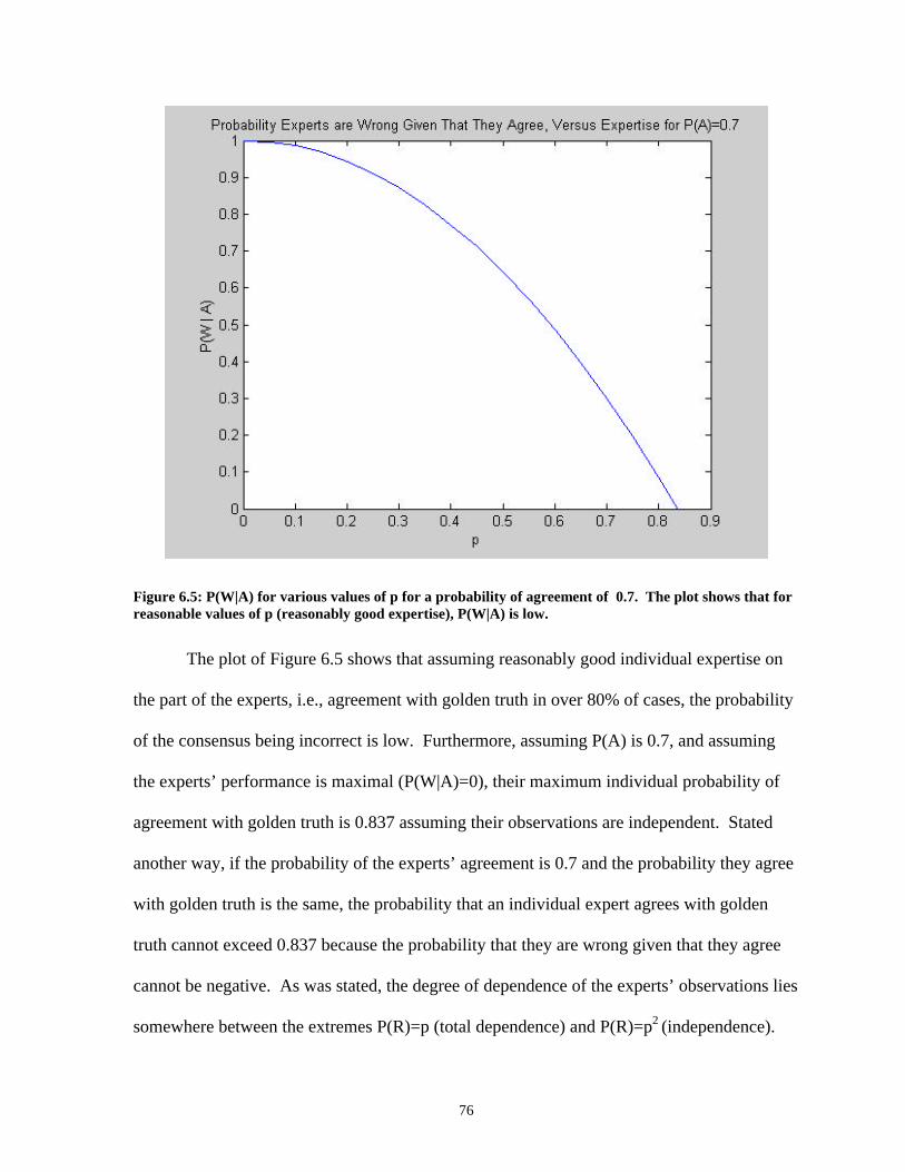
76

Figure 6.5: P(W|A) for various values of p for a probability of agreement of 0.7. The plot shows that for reasonable values of p (reasonably good expertise), P(W|A) is low.

The plot of Figure 6.5 shows that assuming reasonably good individual expertise on

the part of the experts, i.e., agreement with golden truth in over 80% of cases, the probability

of the consensus being incorrect is low. Furthermore, assuming P(A) is 0.7, and assuming

the experts’ performance is maximal (P(W|A)=0), their maximum individual probability of

agreement with golden truth is 0.837 assuming their observations are independent. Stated

another way, if the probability of the experts’ agreement is 0.7 and the probability they agree

with golden truth is the same, the probability that an individual expert agrees with golden

truth cannot exceed 0.837 because the probability that they are wrong given that they agree

cannot be negative. As was stated, the degree of dependence of the experts’ observations lies

somewhere between the extremes P(R)=p (total dependence) and P(R)=p2 (independence).

77

For example, if P(R)=p3/2, then the maximum value of p is 0.788 assuming P(A)=0.7 and

letting P(W|A)=0. The probability p=0.837 will be used as a measure of human performance

on this task for comparison with the classification results presented below because it is an

upper bound on the experts’ individual performance.

Table 6.2: Cases where a consensus was reached by two human experts on apical regional wall motion. Their detailed analyses are given in columns 2 and 3, and the consensus is given in column 4. Column 5 is the apical wall motion class used in statistical classification experiments. The experts evaluated the cases blindly and their consensus was defined by independent analysis of their independent results.

Case Number

Physician 1 Diagnosis

Physician 2 Diagnosis

Consensus Apical Wall Motion Class

5781 Normal Normal Normal Normal 57811 Normal Normal Normal Normal 57831 Normal Normal Normal Normal 5784 Normal Normal Normal Normal 57853 Normal Normal Normal Normal 57858 Latero-Basal Mild

Hypokinesis Normal Normal Apical Normal

57862 Normal Normal Normal Normal 57922 Normal Normal Normal Normal 57926 Latero-Apical

Mild Hypokinesis Infero-Apical Severe Hypokinesis Septal-Apical Mild Hypokinesis

Apical Hypokinesis

Apical Hypokinesis

Abnormal

57946 Normal Normal Normal Normal 5799 Latero-Apical

Moderate Hypokinesis

Apical Hypokinesis Lateral Akinesis

Apical Hypokinesis

Abnormal

58016 Infero-Apical Moderate Hypokinesis

Apical Hypokinesis

Apical Hypokinesis

Abnormal

5803 Normal Normal Normal Normal 58040 Latero-Apical

Severe Hypokinesis

Mild Global Hypokinesis

Apical Hypokinesis

Abnormal

58042 Latero-Apical Severe Hypokinesis

Mild Global Hypokinesis, most prominent at Apex

Apical Hypokinesis

Abnormal

58056 Septal-Apical Moderate Hypokinesis

Apical and Septal Hypokinesis

Apical Hypokinesis

Abnormal

58061 Septal-Apical Moderate

Mild Apical Hypokinesis

Apical Hypokinesis

Abnormal

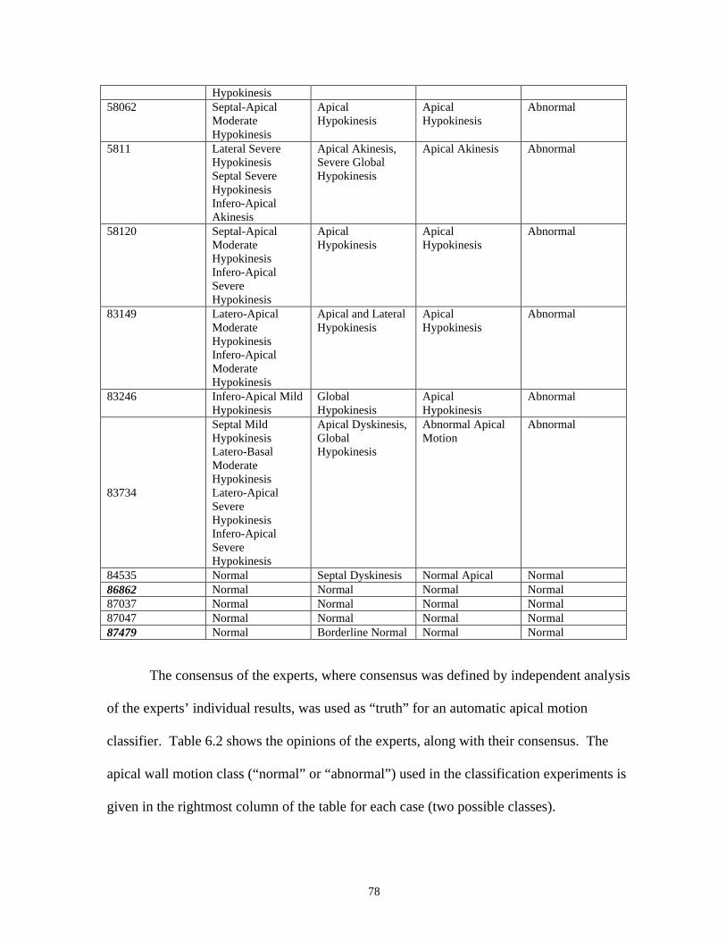
78

Hypokinesis 58062 Septal-Apical

Moderate Hypokinesis

Apical Hypokinesis

Apical Hypokinesis

Abnormal

5811 Lateral Severe Hypokinesis Septal Severe Hypokinesis Infero-Apical Akinesis

Apical Akinesis, Severe Global Hypokinesis

Apical Akinesis Abnormal

58120 Septal-Apical Moderate Hypokinesis Infero-Apical Severe Hypokinesis

Apical Hypokinesis

Apical Hypokinesis

Abnormal

83149 Latero-Apical Moderate Hypokinesis Infero-Apical Moderate Hypokinesis

Apical and Lateral Hypokinesis

Apical Hypokinesis

Abnormal

83246 Infero-Apical Mild Hypokinesis

Global Hypokinesis

Apical Hypokinesis

Abnormal

83734

Septal Mild Hypokinesis Latero-Basal Moderate Hypokinesis Latero-Apical Severe Hypokinesis Infero-Apical Severe Hypokinesis

Apical Dyskinesis, Global Hypokinesis

Abnormal Apical Motion

Abnormal

84535 Normal Septal Dyskinesis Normal Apical Normal 86862 Normal Normal Normal Normal 87037 Normal Normal Normal Normal 87047 Normal Normal Normal Normal 87479 Normal Borderline Normal Normal Normal

The consensus of the experts, where consensus was defined by independent analysis

of the experts’ individual results, was used as “truth” for an automatic apical motion

classifier. Table 6.2 shows the opinions of the experts, along with their consensus. The

apical wall motion class (“normal” or “abnormal”) used in the classification experiments is

given in the rightmost column of the table for each case (two possible classes).

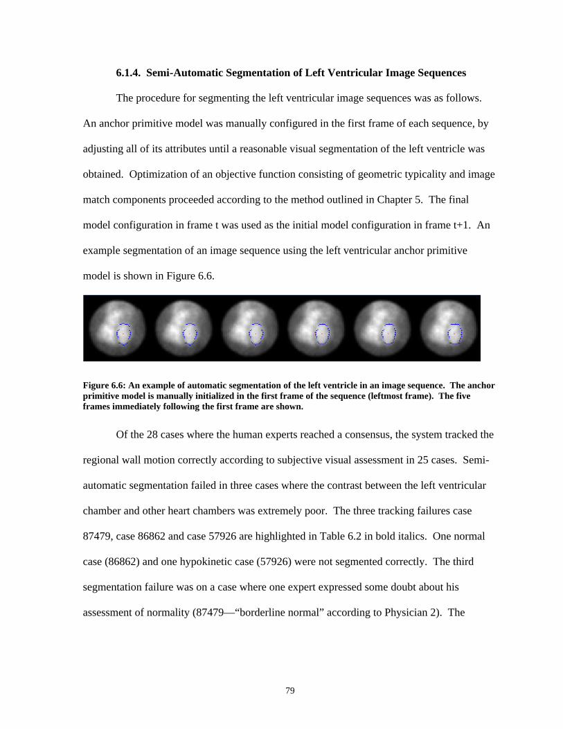
79

6.1.4. Semi-Automatic Segmentation of Left Ventricular Image Sequences

The procedure for segmenting the left ventricular image sequences was as follows.

An anchor primitive model was manually configured in the first frame of each sequence, by

adjusting all of its attributes until a reasonable visual segmentation of the left ventricle was

obtained. Optimization of an objective function consisting of geometric typicality and image

match components proceeded according to the method outlined in Chapter 5. The final

model configuration in frame t was used as the initial model configuration in frame t+1. An

example segmentation of an image sequence using the left ventricular anchor primitive

model is shown in Figure 6.6.

Figure 6.6: An example of automatic segmentation of the left ventricle in an image sequence. The anchor primitive model is manually initialized in the first frame of the sequence (leftmost frame). The five frames immediately following the first frame are shown.

Of the 28 cases where the human experts reached a consensus, the system tracked the

regional wall motion correctly according to subjective visual assessment in 25 cases. Semi-

automatic segmentation failed in three cases where the contrast between the left ventricular

chamber and other heart chambers was extremely poor. The three tracking failures case

87479, case 86862 and case 57926 are highlighted in Table 6.2 in bold italics. One normal

case (86862) and one hypokinetic case (57926) were not segmented correctly. The third

segmentation failure was on a case where one expert expressed some doubt about his

assessment of normality (87479—“borderline normal” according to Physician 2). The

80

classification experiments discussed below were on the 25 cases where semi-automatic

anchor primitive based segmentation was successful.

6.1.5. Feature Selection and Hidden Markov Models for Left Ventricular Regional Wall Motion Classification

A hidden Markov model (HMM) was used to represent each class, one for “normal

apical motion” and one for “abnormal apical motion.” (HMM’s are described in more detail

in Chapter 4.) Using the “truth” shown in Table 6.2, models were trained using a leave-one-

out training procedure. It is not possible to make precise statements about the generalization

capability of the system based on the leave-one-out analysis because of the following

limitations. The leave-one-out set is relatively small, so there may be aspects of the general

population not seen in the leave-one-out set. Thus, training and testing on larger populations

may yield different performance. Also, feature selection was tuned based on the leave-one-

out set, so it may not generalize. This is because selected features yield different models for

each leave-one-out case, and the models corresponding to the selected features could be

different for a different (larger) training population. That said, the leave-one-out results are

good for the data at hand, which is suggestive of good capability in general.

To select features for recognition, classification experiments were run on each feature

in isolation (a single feature extracted per frame). Results for the single feature per frame

experiments are presented in Table 6.3. For the results of Table 6.3, hidden Markov models

with a small number of parameters were chosen to represent each class, namely models with

three states and two Gaussian mixture components per state. The intuition behind choosing

three states was that one would represent systole (left ventricle contraction), one would

represent diastole (left ventricle expansion), and one would represent the transition between

systole and diastole (end-systole). Two Gaussian mixture components per state were chosen

81

to keep the number of model parameters small because of the relatively small number of

training cases considered. It is typical in sequence classification applications like speech and

handwriting recognition to use more than one Gaussian per state—often many Gaussians per

state are used.

Feature S1 S2 α1 α2 α3 α4 dS1 dS2 dα1 dα2 dα3 dα4 Errors 9 20 15 12 13 14 12 9 18 10 6 14

Table 6.3: Number of classification errors for each individual left ventricle anchor primitive feature. Hidden Markov Model Number of States = 3, Number of Gaussians per State = 2.

A greedy approach to combining individual features into feature vectors was taken based on

the single feature experiments. The greedy approach selected the features with the best

classification performance when taken alone and combined them into multidimensional

feature vectors. The features with the minimal number of classification errors were

combined, according to Table 6.4.

Features Errors S1, dS2 7 S1, dS2, dα3 10 dS2, dα3 9 S1, dα3 8

Table 6.4: Number of classification errors using a greedy selection of features based on Table 6.3. Hidden Markov Model Number of States = 3, Number of Gaussians per State = 2.

The conclusion from the experiments of Table 6.4 was that the greedy choice of S1,

dS2, dα3 did not yield good results because of insufficient training data (too many model

parameters given the training set size). It was thus decided to decrease the complexity of the

models of each state by reducing the number of Gaussians per state from two to one. Because

this choice reduces the number of mixture model parameters by one half, the number of

states in each hidden Markov model can be doubled without substantially increasing the

number of model parameters found when there are two Gaussians per state.

82

Table 6.5 presents the results for various combinations of features, using one

Gaussian per state, for various numbers of states. The best result achieved was 5 errors out

of 25 sequences. This was achieved using (dS2, S1) feature vectors from each frame with

each model having 9 states or 15 states, and also achieved using (S1) alone from each frame

with each model having 12 states or 13 states. It was expected that a feature vector involving

dS2 would yield good apical motion classification. It is somewhat surprising that S1 alone

yields good apical motion classification; however, the apical, septal, and lateral walls are of

course connected by muscle tissue thus motion in one region influences motion in others.

Most of the abnormal apical motion cases correspond to some degree of hypokinetic

motion. Thus, it was observed that cases 5811 and 83734 were potential outliers with respect

to the abnormal motion class. In case 5811, both physicians suspected apical akinesis. In

case 83734, one physician suspected apical dyskinesis, in addition to global hypokinesis.

However, in all experiments reported in Table 6.5 for various numbers of hidden Markov

model states for the (dS2, S1) feature set, cases 5811 and 83734 were classified correctly.

This suggests that based on case 5811, akinesis was better represented by the “abnormal

apical motion” model, formed mainly on the basis of hypokinetic cases, because it always

yielded a higher probability of case 5811 given the abnormal apical motion model in the

leave-one-out experiments. This corresponds to intuition that says that akinesis—no wall

motion—is more like hypokinesis—sluggish motion—than it is like normal motion. The fact

that the physician who mentioned dyskinesis of case 83734’s apical motion also gave an

observation of global (for all regions) hypokinesis indicates he could have been admitting the

possibility of hypokinetic apical motion rather than dyskinetic apical motion. Hypokinetic

apical motion is suggested by the classifier because case 83734 was never misclassified for

83

the (dS2, S1) feature set; thus case 83734 agreed well with the “abnormal apical motion”

class trained mainly on cases where there was a consensus of experts of apical hypokinesis.

Features # States

dS2, S1 dS2, S1, dα3

DS2, dα3 S1, dα3 dS2 dα3 S1

3 8 4 8 10 5 10 9 6 8 7 7 7 11 8 6 7

9 5 8 11 10 16 8 6 10 6 6 11 8 6 12 7 5 13 7 5 14 6

6 15 5 10 10 16 6 16 7 17 9

Table 6.5: Number of classification errors for various combinations of features for various numbers of states per hidden Markov model. Best classification performance is 5 errors, achieved in several different ways. Number of Gaussians per state = 1.

6.1.6. Comparison of Left Ventricular Classification Results to Other Work

As in this work, Sychra attempted to automate classification of left ventricular

regional wall motion in gated blood pool images.1 Sychra achieved about 80% classification

accuracy (70 cases) on his training set when distinguishing normal motion from hypokinetic

motion. Two of his classes represented normal motion and three of his classes represented

degrees of hypokinesis. He defined “acceptable agreement” with the physician consensus as

a maximum of one class difference from the consensus. Using this definition of acceptable

agreement, he achieved an average of 86% pixel accuracy for normal cases and an average of

73% accuracy for hypokinetic cases. These reported accuracies are classification accuracies

on his training set.

84

Based on the upper bound derived above, the maximal theoretical performance of

each expert who classified the data used in this study was p=0.837. 80% classification

accuracy (25 cases) where truth is taken to be consensus of two experts is achieved by the

anchor primitive/hidden Markov model system in a leave-one-out analysis when

distinguishing normal apical motion from abnormal apical motion. The human’s task was

more detailed that the system’s task, however, because the number of regions and the number

of wall motion classes considered by the experts were larger than those considered by the

system. As was noted, because of the small set size, leave-one-out analysis is suggestive of

good performance but does not give a precise indication of generalization capability.

6.2. Computer Lipreading

Computer lipreading is automatic classification of lip image sequences. Computer

lipreading was discussed in Chapter 3. The point of computer lipreading is to augment

acoustic speech recognizers in noisy environments, as was discussed in Chapter 1 and in

Chapter 3. It has been shown that systems that combine computer lipreading and acoustic

speech recognition outperform acoustic speech recognition systems in noisy environments.

6.2.1. Anchor Primitive for Lips

An anchor primitive was designed to represent the lips. The lip anchor primitive used

three parametric curves. One parametric curve each for the two halves of the upper lip and

one parametric curve for the lower lip were used. Anchor primitive attributes include the

distances, represented by Si, i=1,…,5, in Figure 6.7 (repeated from Chapter 5 for the reader’s

convenience), to the parametric curve control points from the center point. Other attributes

include the (X,Y) location of the center of the anchor primitive representing the middle of the

mouth, and angles that when combined with the distances specify the locations of each of the

85

control points. There are 12 lip anchor primitive attributes. The Ik values, k=1,…,3, of

Figure 6.7 are intensity features implied by the anchor primitive model, not geometric

attributes of the model. They are not used for anchor primitive based segmentation but are

candidate statistical features for anchor primitive based classification.

(X,Y) S1

S2S4S3

S5

I1 I2I3

a

b

c

Figure 6.7: Schematic of the Lip Anchor Primitive. S1 and S3 are distances from the center of the primitive to points on the mouth (center to corners – S1, center to midpoint of upper lip – S3). S2, S4, and S5 are distances from the center of the primitive to control points for parametric curves representing the lip boundaries. Example control points for the quadratic representing the upper right portion of the lip boundary are given by a, b, and c. Similar quadratics defined by the anchor primitive attributes represent the upper left and lower boundaries as well. Angles O1, O2, O3, O4 and O5 (not pictured) corresponding to S1, S2, S3, S4 and S5 precisely locate the control points for the 3 parametric curves representing the lip boundaries. I1, I2 and I3 are intensity values at the center of the mouth (I1) and a +/- offset from the center of the mouth that is proportional to S1 (I2 and I3).

6.2.2. Lip’s Statistical Features Implied by the Anchor Primitive Model

Because it was assumed that lip image sequence classification should be independent

of the translation and global rotations of the mouth during speech, the position and angle

attributes of the lip anchor primitive were not used as features for classification. Instead it

was felt that the control point distances from the center of the anchor primitive and intensity

values around the center of the mouth would be most useful for classification. Inter-frame

changes in these values were used as features for statistical classification as well. A list of

the features used for classification is given in Table 6.6.

86

Feature S1 S2 S3 S4 S5 I1 I2 I3 dS1 dS3 dS5 dI1 dI2 dI3

Table 6.6: Features used for lip image sequence classification. SX denotes distance to a parametric curve control point as indicated in Figure 6.7 above. dx is the inter-frame change in x. I1, I2, and I3 are intensity values collected based on the anchor primitive location, as illustrated in the figure above.

6.2.3. Lip Image Data

The Tulips 1 database of isolated digits2 was used for all computer lipreading

experiments. It is composed of image sequences from 12 speakers speaking each of the first

four English digits (“one,” “two,” “three,” “four”) twice, for a total of 96 sequences. Speaker

independent recognition experiments were performed using a cross-validated, “leave-one-

speaker-out,” procedure. From Luettin’s description of the database:3

The subjects were asked to talk into a video camera and to position themselves so that their lips were roughly centered in a feed-back display. The gray-scale images were digitized at 30 frames/s, 100x75 pixels, 8 bits per pixel. The database contains a total of 934 images and consists of speakers with different ethnic origins, [9 males and 3 females], some with makeup or facial hair and different illumination. An example of a sequence from the database is shown in Figure 6.8. The low

contrast between the lower lip boundary and the face is typical of images in the database.

This database was of interest because other researchers have published classification

performance results on it.

87

Figure 6.8: An example of a sequence from the Tulips 1 lip image sequence database. The low contrast between the lower lip boundary and the face is typical of image sequences from the database. Time 0 is at the upper left corner of the figure. Time increases from left to right and from top to bottom.

6.2.4. Semi-Automatic Segmentation of Lip Image Sequences

Semi-automatic segmentation of the lip image sequences using anchor primitives was

attempted. The procedure was to find initial segmentations of the first and last frame of each

sequence manually by adjusting the anchor primitive parameters (there are 12 parameters-2

positional parameters, 5 scales and 5 orientations). Optimization of an objective function

consisting of geometric typicality and image match components proceeded according to the

method outlined in Chapter 5. After initial manual adjustment of all anchor primitive

parameters, optimization was run only over distances between the anchor primitive center

88

point and control points. The final anchor primitive configuration in frame t was used as the

initial configuration in frame t+1. Segmentation was also run backwards so that the optimal

anchor primitive configuration in frame t was the initial anchor primitive configuration in

frame t-1, using the manual segmentation of the last frame as the starting point for the

backwards sequence segmentation. For each frame, the forward or backwards segmentation

was selected according to the algorithm given in Chapter 5. An example of semi-automatic

segmentation achieved when using this method is given in Figure 6.9.

Figure 6.9: Anchor primitive based semi-automatic segmentation of a lip image sequence “four” from talker “Anthony.” The discontinuity observed between frames 3 and 4 above (upper right corner) is typical of the digit “four” for many speakers, because the lower lip accelerates rapidly following release of the plosive.

89

For the classification experiments discussed below, 74 semi-automatic segmentations

were used and 22 manual segmentations were used, where the anchor primitives were

manually placed in each frame of 22 image sequences. Semi-automatic segmentation was

hindered by the facts that shadows severely limited contrast between the lower lip and the

face in many images and that the lower lip boundary extended beyond the image boundary in

some cases.

6.2.5. Feature Selection and Hidden Markov Models for Computer Lipreading

All classification experiments described below were speaker independent, leave-one-

speaker-out experiments, which were the same as those conducted by Luettin. To select

features for recognition, classification experiments were run on each feature in isolation (a

single feature extracted per frame). Results for the single feature experiments are presented

in Table 6.7. Then a greedy approach to combining individual features into feature vectors

was taken. The features with the minimal number of classification errors were combined

(ignoring S2 and S4), according to Table 6.8. Classification results for various feature

vectors are presented in Table 6.8. The best result of 10 out of 96 errors was achieved using

(S1, dS1, S3, dS3, S5, dS5, I1) from each frame. The selected set of features correspond well

to intuition that says normalized distances from the center of the mouth to the middle of the

upper lip, middle of the lower lip, and corners of the mouth and inter-frame changes in those

values describe lip movement during speaking. In addition, normalized intensity feature I1

from the anchor primitive center location was an important feature as well, as was expected

based on the literature that showed the importance of the visibility of the teeth and tongue to

lipreading.

90

Feature S1 S2 S3 S4 S5 I1 I2 I3 dS1 dS3 dS5 dI1 dI2 dI3 Errors 45 49 52 47 42 42 53 56 50 51 50 57 57 53

Table 6.7: Number of classification errors for each individual lip anchor primitive feature. Leave-one-speaker-out classification experiments were run using a single feature extracted from each frame of each image sequence. Number of States = 4, Number of Gaussians per State = 2.

Features Errors

(4 States) Errors

(3 States) Errors

(5 States) S5, I1 28 S5, I1, S1 16 S5, I1, S1, dS1 14 S5, I1, S1, dS1, dS5 13 S5, I1, S1, dS1, dS5, dS3 12

S5, I1, S1, dS1, dS5, dS3, S3 10 16 16 S5, I1, S1, dS1, dS5, dS3, S3, dI3 14 S5, I1, S1, dS1, dS5, dS3, S3, dI3, I2 15

Table 6.8: Number of classification errors using a greedy selection of features based on Table 6.7 without considering S2 and S4. Number of Gaussians per State = 2.

6.2.6. Comparison of Lip Image Sequence Classification Results to Other Work

The 10 out of 96 errors result is not very different from the 9 out of 96 errors

achieved as their best-reported result by Luettin and Thacker on the same database using the

same leave-one-speaker-out analysis technique.2 The result using the lip anchor primitive

based approach was achieved using 7 features including shape and intensity features and

inter-frame changes in shape features. Luettin’s best-reported result was achieved using 10

features including shape and intensity features and their inter-frame changes. The number of

errors of the two approaches with 95% confidence intervals are shown in Figure 6.10. It

should also be noted that Luettin and Thacker were able to achieve 10 errors on the task

using 3 intensity features only using an approach based on the work of Taylor and Cootes.

However, on a more difficult task, an intensity-only approach might not yield good

performance.

91

Number of Errors with 95% Confidence Intervals

02468

1012141618

10 Features (Luettin) 7 Features (Clary)

Figure 6.10: Comparison between numbers of classification errors on the Tulips 1 database (with 95% confidence intervals) and numbers of features for Luettin’s shape and intensity based approach and Clary’s anchor primitive based approach.

The lip anchor primitive result is also similar to the 89.93% classification accuracy

achieved by humans with no lipreading knowledge who were asked to classify the same

sequences. Hearing impaired humans with lipreading knowledge achieved 95.49% accuracy

on this database.1,2

The approach of Luettin and Thacker includes a more automated lip segmentation

solution. The purpose of this work was to evaluate the anchor primitive model itself as a

basis for feature extraction, rather than any particular combination of model to image match

and geometric typicality. To produce an automated segmentation and classification method,

aspects of Luettin’s segmentation approach could be combined with the anchor primitive

model, including the use of a more robust statistical model of boundary intensities for model

to image match measurement, following the work of Taylor and Cootes. More will be said

about this in Chapter 7, Future Work. The limitations discussed previously of leave-one-out

92

analysis regarding conclusions about generalization capability also apply to the computer

lipreading results.

6.3. Conclusions Regarding Anchor Primitives

Anchor primitive attributes can be used as intuitive and easy to compute geometric

features for statistical classification of image object evolution in image sequences. The

features are intuitive because they are based directly on geometric aspects of the anchor

primitive model. The features are easy to compute after image segmentation because they

are obtained directly from anchor primitive attributes or differences in those attributes over

time. These features are more intuitive and easier to compute than pixel based features like,

for example, those based on filtering (derivative of Gaussian, etc.), optic flow features, other

functions of pixel time activity, or principal components analysis on functions of intensity

values.

The anchor primitive model provides a global representation of an object by modeling

its landmarks and by providing local representations of object parts via the use of analytic

boundary representations. Anchor primitives are designed to be used to establish

correspondence at large spatial scale. As was explained, using naturally occurring

symmetries between corresponding locations allows anchor primitives to be consistently

placed across a population of image objects.

While global, anchor primitives can allow consistent placement of associated sub-

models that model an image object in a more detailed way. For example, if anchor primitives

are used in conjunction with m-reps, it may be useful to constrain a medial atom to have the

same location as the anchor primitive center point location (the “anchor primitive medial

atom”). If an m-rep is used to model an image object in more detail in the direction of one of

93

the anchor primitive’s corresponding locations, it may be useful to place a constant number

of equally spaced medial atoms between the anchor primitive medial atom and the anchor

primitive corresponding location along the distance and direction to the corresponding

location. (Assume the distance and direction of each of the anchor primitive’s corresponding

locations is given by the anchor primitive model.) This constraint during m-rep placement

would provide useful correspondence between medial atoms if the important

correspondences are captured by the anchor primitive.

Because anchor primitives take advantage of object symmetry to define a center point

location, if a reference direction is defined, then an object-centric coordinate system can be

defined for 2D image objects. The object-centric coordinate system is useful for making

shape comparisons among image objects segmented via anchor primitives. The reference

direction could be defined based on the location of the most stable corresponding place based

on a training population for the image object under consideration. Defining the most stable

corresponding place is discussed further in Chapter 7.

Given accurate image segmentations, a small number of anchor primitive implied

features—a concise feature set—can provide accurate hidden Markov model based

classification of image sequences in leave-one-out analysis. A small number of features

means that a smaller training set can potentially yield accurately estimated models that have

good generalization performance. Also, the computational complexity of estimating

Gaussian distributions with full covariance matrices is quadratic in the dimensionality of the

feature space. Thus, the fact that anchor primitives can yield useful features in a feature

space of low dimensionality means more computationally efficient training and potentially

more accurate statistical classification using hidden Markov models.

94

Using hidden Markov models for time series modeling has implications for time scale

selection. With a constant number of Gaussians per state, if a representation with a large

number of states gives good classification performance, it is suggested that fine temporal

scale details are important to classification. However, care must be taken to ensure that all

states are truly useful to the representation by examining the sequence of visited states using

standard techniques. It may be necessary to interpolate the training data to produce a larger

number of frames to ensure that an adequate amount of training data is available for a

representation with a large number of states. If a representation with a smaller number of

states gives good classification performance, then fine temporal scale details may not be

relevant for classification. In this case, one might consider windowing the data across time

to yield a smaller number of input frames.

Because a segment-then-recognize approach was taken to classification in this work,

with segmentation considered separately from classification, semi-automatic segmentation

results presented in this chapter have implications for segmentation using anchor primitives

of static images, not only time sequences of images. The studied blood pool images are quite

noisy, and anchor primitive based segmentation of them was largely successful. Because

image measurements are made at places where intensity information is likely to be consistent

with a training set, model to image match is likely to be maximal where expected. Because

geometric typicality involves relationships between corresponding places that are likely to be

consistent across different image objects and because anchor primitives use analytic

representations of curvilinear segments, deformable model based segmentation is adequately

constrained.

95

It has been shown that anchor primitives can provide an efficient image object

representation for deformable model based image segmentation. Anchor primitives make it

possible to compute model to image match function values only in corresponding locations

rather than around the entire boundary of an image object as is the case for many b-rep

deformable models. The left ventricle anchor primitive of this work required image

measurements in four key locations only. In addition, anchor primitives via the use of

symmetries can provide a search space of lower dimensionality for deformable model

placement than other representations. The best performing b-rep in terms of classification

accuracy used by Luettin and Thacker to model the lips required a search space of 14

dimensions for model placement. The anchor primitive for the lips evaluated in this work

has 12 parameters. However, Luettin’s best b-rep modeled both the inner and outer contour

of the lips.

What has been shown is that carefully designed anchor primitives where center

locations and corresponding locations are hand selected can provide useful features for

statistical classification. Methods for computer aided anchor primitive design should be

developed and evaluated. This subject will be addressed more fully in Chapter 7.

In summary, it has been shown that anchor primitives can provide concise and

accurate statistical features for image sequence classification, producing reasonable

classification accuracy in leave-one-out analysis and computationally efficient statistical

classification. Anchor primitives could be useful for image segmentation and image object

comparison in general, a statement that can be more thoroughly studied in future research.

96

6.4. Contributions

A summary of how the contributions of the dissertation outlined in Chapter 1 are

supported by the experimental results is given here.

• A novel medial primitive called an anchor primitive has been introduced. The

anchor primitive is a correspondence maintaining primitive placed in each

frame of an image sequence using the continuity of the sequence. Semi-

automatic segmentation of image sequences using anchor primitives was

successful in the majority of cases considered in this work. It was shown that

given accurate image segmentations, classification performance using anchor

primitives as a basis for statistical features was similar to that found in the

literature for the computer lipreading task. Anchor primitives in image

sequences effectively generate shape parameter sequences. Thus, accurately

placed anchor primitives provide consistent model to image object feature

correspondence needed for the analysis of the shapes found in the example

image sequences and classification of their evolution. There are obvious

segmentation techniques for model to image match and geometric typicality

measurement that should be incorporated into the anchor primitive framework

to yield automatic segmentation. Some of these are discussed in Chapter 7.

• Because statistical features for classification can come directly from anchor

primitive attributes or inter-frame changes in attributes, anchor primitives

supply features for statistical classification that are easy to compute. Because

anchor primitives capture the geometry of the modeled shape in a holistic and

natural way in a few parameters, anchor primitive attributes are intuitive.

97

Intuitive geometric features enable discussion of classification results in

medically relevant terms.

• A method was described that uses anchor primitive based features as inputs to

hidden Markov models for statistical classification.

• For 25 example cases, anchor primitive based features and hidden Markov

models provided left ventricular regional wall motion classification accuracy

in leave-one-out analysis suggestive of similarity to that of human experts.

The human experts agreed with one another 70% of the time, and the semi-

automatic classification method agreed with the experts on 80% of cases

where the human experts agreed. It should be noted, however, that the

analysis of the human experts was more challenging than the semi-automatic

analysis because the experts considered more “classes”—more wall regions

and types and degrees of abnormality.

• For 96 example image sequences, and given accurate image sequence

segmentations, anchor primitive based features and hidden Markov models

provided computer lipreading accuracy similar to that found in the literature

using leave-one-speaker-out analysis.

• Distances from the anchor primitive center point location and anchor primitive

model point locations and changes in those distances were useful features for

statistical classification via leave-one-out analysis of image object shape

evolution.

Through empirical studies of anchor primitive based segmentation and statistical

classification using anchor primitive implied features, the contributions of the dissertation

98

outlined in Chapter 1 have been supported. The following chapter makes suggestions for

interesting future research directions.

99

1. J.J. Sychra, D.G. Pavel, and E. Olea, “Fourier Classification Images in Cardiac

Nuclear Medicine,” IEEE Transactions on Medical Imaging, Vol. 8, No. 3, Sept. 1989. 2. J.R. Movellan, “Visual Speech Recognition with Stochastic Networks,” in

Advances in Neural Information Processing Systems, G. Tesauro, D. Touretzky, and T. Leen, eds., Vol. 7, Cambridge, MA: MIT Press, 1995.

3. J. Luettin and N.A. Thacker, “Speechreading using Probabilistic Models,”

Computer Vision and Image Understanding, Vol. 65, No. 2, 1997, pp. 163-178.

Chapter 7

Future Work

There are many promising directions based on this work that can be explored. The

directions fall into two major categories: 1) improving the current implementations of anchor

primitives including by extension of the theory of anchor primitives and 2) further

applications of anchor primitives. Both categories apply to static image segmentation and

statistical feature extraction as well as image sequence segmentation and feature extraction

using anchor primitives.

Because a segment-then-recognize approach was taken to classification in this work,

with segmentation considered separately from classification, semi-automatic segmentation

results presented in Chapter 6 are suggestive of capability for segmentation of static images

in general using anchor primitives. As was stated in Chapter 6, because image measurements

are made at places where intensity information is likely to be consistent with a training set,

model to image match is likely to be maximal where expected. Because geometric typicality

involves relationships between corresponding places that are likely to be consistent across

different image objects, segmentation is adequately constrained. Research on improved

segmentation methods based on this idea might incorporate the aspects discussed in this

chapter.

101

Image segmentation in many cases in this work involved manual steps, including

initializing the object tracking algorithms. The purpose of the work was to prove that anchor

primitives could produce useful statistical features for classification of shape evolution in

time sequences of images, rather than to prove that automatic anchor primitive based image

segmentation could be accomplished. Some, if not all, of the manual steps could be

eliminated by using more robust model to image match measures. Following the active

appearance model approach of Cootes and Taylor to computing model to image match would

be useful. An alternative, and perhaps more effective, approach is the multiscale boundary

profile approach of Ho and Gerig.1 The first place this author saw multiscale model to image

match measurement was in the work of Coggins, and it was inspirational in this regard.

Anchor primitives were defined in Chapter 5. They consist of a center point location,

deformable models of corresponding locations, and relationships between the models of

corresponding locations. An interesting future study is to identify ways to build anchor

primitive models. Two issues are critical. One is identifying the anchor primitive center

point location. The other is identifying corresponding places across training populations of

image objects. Anchor primitives model corresponding places using parametric curves or

deformable m-reps and use the geometric relationships between the corresponding places to

measure geometric typicality.

Identifying a center point location can be performed manually by the model builder.

The model builder can choose to examine the largest scale medial tracks of a representative

image object or mean object representing a training population. The center point location

can be specified as the spatial intersection point of the largest scale medial tracks.

Alternatively, the model builder may examine extremal boundary points of a representative

102

image object or mean object representing a training population and specify the center point as

the centroid of the extremal points.

Identifying corresponding places across training populations is a significant area for

further research that has implications not only for anchor primitive model building but also

for deformable model based segmentation in general. By definition, places that are said to

exhibit correspondence have unique but consistent intensity and shape properties across

populations of image objects. To find corresponding places, I recommend that an

unsupervised statistical technique such as K-Means clustering be performed on shape and

intensity features and neighboring primitive (boundary or medial) relationships of a training

population of image objects. The most compact clusters represent the corresponding places.

An algorithm could proceed as follows:

• Perform deformable m-rep segmentation using a dense sampling of the medial

manifold(s) of a training population.

• Run k-means clustering (or another statistical clustering technique) on the

medial atom attributes together with intensity features that correspond to the

medial atoms and neighboring medial atom relationships. The k-means

algorithm will need to be modified to incorporate the Lie group geodesic

distance metric and Lie group based Gaussian distribution definitions for m-

reps.

• Scatter plot medial atom locations corresponding to the most compact clusters

on a representative object of the training population. Use the cluster labels as

labels on the scatter plot. Viewing the scatter plot is to account for cases

where multiple corresponding locations have shape, intensity and neighbor

103

relationship properties similar enough to cause them to belong to the same

cluster.

• If the scatter plot of the medial atom locations from the training population

corresponding to the most compact clusters produces a reasonable number of

corresponding places, select those places to model with anchor primitive

parametric curves or deformable m-reps.

• In a place where the neighboring corresponding locations are relatively far

apart, use parametric curves to model the corresponding location, because

immediately neighboring locations do not exhibit correspondence by the

cluster analysis implying that boundary information is potentially more

consistent in the area versus medial information.

• In a place where there is a dense collection of neighboring corresponding

locations, use a deformable m-rep to model the corresponding location

because the dense collection of neighboring corresponding locations

represents a stable figure.

• In addition, if the trace of the covariance matrix of the intensity features from

a particular corresponding location is smaller than the trace of the covariance

matrix of the m-rep features, consider using a curve to model the

corresponding place. If covariance matrices from the intensity features of the

two boundary places corresponding to the medial atom at the corresponding

location are considered separately, it could be decided to use a curve to

represent one boundary place but not the other based on the traces of the

covariance matrices.

104

• If the trace of the covariance matrix of the m-rep features is smaller than the

trace of the covariance matrix of the intensity features, consider using an m-

rep to model the corresponding place.

Correspondence of modeled locations across image objects is critical to consistent

statistical feature extraction. Pizer et al. have made a major contribution by referring to any

location in a 3D image in object medial manifold relative (u,v,t) coordinates. (u,v,t) are

consistently defined across image objects based on a medial surface. A similar formalism

can be developed for anchor primitives. A reference direction can be defined (?=0) based on

the most stable corresponding place given by the cluster analysis above. Any place in a 2D

image with an object defined by an anchor primitive can then be described in terms of an

object-centric angle ?. Because there may not be a 1-to-1 correspondence between ? and the

boundary of an image object, a multi-scale approach to using the anchor primitive based

coordinate system for object comparisons could be taken. For example, ? could be used to

make global comparisons between corresponding figures (corresponding places) in an anchor

primitive model (i.e., comparison of figure locations), and m-rep (u,t) coordinates could then

be used to make figure-to-figure boundary comparisons between corresponding features.

As was mentioned, an approach to spatio-temporal image segmentation is to consider

an N+1 dimensional image segmentation technique for N-D image objects evolving over

time, basically treating time as another dimension. Another way to incorporate time

information into the segmentation process is to make segmentation dependent on class

membership. That is, for each class there is a separate segmentation procedure. This

procedure could involve including the probability that a particular hidden Markov model

(representing a particular class) generated an observation sequence up to the current frame in

105

the objective function for image segmentation. The training algorithm would proceed as

follows. Start with a segmentation algorithm that is the same for all classes (as before)—

optimize image match and geometric typicality. Use the segmentations produced by the

algorithm to train initial hidden Markov models for each class. Re-segment using class

dependent segmentation, by including the probability that the class’s initial HMM generated

the observation sequence up to the current frame in the objective function. Using the new

segmentations for every class, re-train HMM’s for each class. Iterate until performance is

optimized. I call this new term in the posterior function to be maximized “evolution

typicality.” When a new sequence is to be classified, it is automatically segmented a number

of times that is equal to the number of classes, because segmentation is class dependent.

A massive amount of research is being conducted on 3D medical image analysis.

This is because modern imaging modalities provide information over 3 spatial dimensions

that allows accurate and more complete understanding of the imaged anatomy. Defining

anchor primitives for 3D image objects would provide a stable basis for measuring them and

extracting statistical features from them. The same principles used to define 2D anchor

primitives in this work will apply, including defining the following:

• A center point location

• Salient image object feature locations

• Curve, surface, or medial mesh model parameters

• Constraints on the relationships between image object feature locations.

Many computer vision problems of interest involve occlusion. An image object’s

parts (figures) may move in and out of the view of the imaging device. Occlusion could be

handled by anchor primitive based models by building explicit models of occluded and non-

106

occluded figures. During segmentation, all of the occluded and non-occluded models could

be applied and the chosen model would be the one with the highest posterior probability.

Handling occlusion by building anchor primitives to explicitly model situations when

occlusion occurs is an interesting direction.

Although the anchor primitives considered in this work modeled single figure objects,

anchor primitives can be defined for multi-figure objects. In fact, m-reps for each of the

figures can be linked to an anchor primitive defined object center point location to form a

multi-figure anchor primitive. Building multi-figure anchor primitives would aid in time

sequence applications like gait analysis or gesture recognition.

Because complex motions of the heart like twisting cannot be captured in a single

view by a 2D imaging device, left ventricular analysis is typically performed using a 3D plus

time imaging modality. 3D anchor primitives could provide a stable basis for left ventricular

measurement making, left ventricular wall motion quantification, and left ventricular wall

motion classification from typical 3D plus time cardiac imaging modalities such as gated

SPECT.

Analyzing time sequences of images of anatomical structures to determine the effect

of drug or radiation therapies on them is an interesting direction. It is becoming common

practice to image areas of the anatomy that are expected to undergo change as a result of

therapy. Anchor primitive based techniques can be used to measure and classify shape

changes in these images. Recently an entire issue of IEEE Transactions on Medical Imaging

was devoted to image analysis in drug development.2

Performing independent components analysis or independent geodesic analysis on

attributes of anchor primitive models of lips in motion may have useful applications to facial

107

motion synthesis during synthetic speech. Computer animations of “talking heads” have

recently been used to help deaf children learn to speak and to read lips. See

http://abcnews.go.com/sections/primetime/2020/PRIMETIME_010315_baldi_feature.html for more

information on this application of lip motion modeling.

It has been shown by at least two authors that color information aids lip image

segmentation. Color information could easily be incorporated into anchor primitive models

for lips to improve the model to image match function.

Using a “non-linear principal components analysis” technique like principal geodesic

analysis3 as a basis for statistical feature extraction will prove valuable to many image

oriented classification problems, including image sequence classification. Building statistical

models of features from non-Euclidean space will be important as well.4

This dissertation showed that m-rep inspired primitives known as anchor primitives

provide a useful basis for statistical feature extraction for image sequence classification and

thus suggested significant future research directions. Directions include extensions of the

theory of anchor primitives to interactively build anchor primitive models, handle new

situations and incorporate more powerful statistical techniques, and empirical evaluations of

anchor primitive methods in additional image analysis applications.

108

1. S. Ho and G. Gerig, “Scale-Space on Image Profiles About an Object Boundary,”

Scale Space Conference, July, 2003. 2. M. Sonka and M. Grunkin, “Image Processing and Analysis in Drug Discovery

and Clinical Trials,” IEEE Transactions on Medical Imaging, Vol. 21, No. 10, Oct. 2002. 3. P.T. Fletcher, C. Lu and S. Joshi, “Statistics of Shape via Principal Component

Analysis on Lie Groups,” To Appear in CVPR, 2003. 4. P.T. Fletcher, S. Joshi, C. Lu and S.M. Pizer, “Gaussian Distributions on Lie

Groups and Their Application to Statistical Shape Analysis,” Submitted to IPMI, 2003.

109

BIBLIOGRAPHY H. Blum, “A Transformation for Extracting New Descriptors of Shape,” in Symposium on

Models for Perception of Speech and Visual Form, W. Whaten-Dunn, ed., Cambridge, MA: MIT Press, 1967, pp. 362-380.

F.L. Bookstein, “Linear Methods for Nonlinear Maps: Procrustes Fits, Thin-Plate

Splines, and the Biometric Analysis of Shape Variability,” in Brain Warping, A.W. Toga, ed., San Diego: Academic Press, 1999.

C. Bregler and S.M. Omohundro, “Learning Visual Models for Lipreading,” in Motion-

Based Recognition, M. Shah and R. Jain, eds., Kluwer Academic Publishers, 1997. N.M. Brooke, “Talking Heads and Speech Recognizers That Can See: The Computer

Processing of Visual Speech Signals,” in Speechreading by Humans and Machines: Models, Systems, and Applications, D.G. Stork and M.E. Hennecke, ed., Berlin: Springer-Verlag, 1996, pp. 351-371.

C.A. Burbeck, S.M. Pizer, B.S. Morse, D. Ariely, G.S. Zauberman, and J.P. Rolland,

“Linking object boundaries at scale: a common mechanism for size and shape judgments,” Vision Research, Vol. 36, pp. 361-372.

G.E. Christensen, S.C. Joshi, and M.I. Miller, “Volumetric Transformation of Brain

Anatomy,” IEEE Transactions on Medical Imaging, Vol. 16, No. 6, Dec. 1997. G.J. Clary, S.M. Pizer, D.S. Fritsch, and J.R. Perry, “Left Ventricular Wall Motion

Tracking via Deformable Shape Loci,” in Computer Assisted Radiology and Surgery, Proceedings of the 11th International Symposium and Exhibition, H.U. Lemke, M.W. Vannier, and K. Inamura, eds., Amsterdam: Elsevier Science B.V., 1997, pp. 271-276.

T.F. Cootes and C.J. Taylor, “Active shape models—Smart snakes,” in Proceedings of

the British Machine Vision Conference, Berlin: Springer-Verlag, 1992, pp. 266-275. T.F. Cootes, C.J. Taylor, D.H. Cooper, and J. Graham, “Active shape models—Their

training and application,” Computer Vision and Image Understanding, Vol. 61, No. 1, 1995, pp. 38-59.

T.F. Cootes, C.J. Taylor, A. Lanitis, D.H. Cooper, and J. Graham, “Building and using

flexible models incorporating grey-level information,” in Proceedings of the International Conference on Computer Vision, 1993, pp. 242-246.

E.G. DePuey, “Evaluation of Ventricular Function,” in Clinical Practice of Nuclear

Medicine, A. Taylor and F.L. Datz, ed., New York: Churchill Livingstone, 1991, p. 72.

110

E.G. DePuey, E.V. Garcia, and D.S. Berman, eds., Cardiac SPECT Imaging, Second Edition, Philadelphia: Lippincott Williams and Wilkins, 2001.

R.O. Duda and P.E. Hart, Pattern Classification and Scene Analysis, New York: John

Wiley & Sons, 1973, p. 341. P.T. Fletcher, S. Joshi, C. Lu and S.M. Pizer, “Gaussian Distributions on Lie Groups and

Their Application to Statistical Shape Analysis,” Submitted to IPMI, 2003. P.T. Fletcher, C. Lu and S. Joshi, “Statistics of Shape via Principal Component Analysis

on Lie Groups,” To Appear in CVPR, 2003. A.F. Frangi, W.J. Niessen, and M.A. Viergever, “Three-Dimensional Modeling for

Functional Analysis of Cardiac Images: A Review,” IEEE Transactions on Medical Imaging, Vol. 20, No. 1, Jan. 2001.

A.F. Frangi, D. Rueckert, and J.S. Duncan, “Three-Dimensional Cardiovascular Image

Analysis,” IEEE Transactions on Medical Imaging, Vol. 21, No. 9, Sept. 2002. D.S. Fritsch, S.M. Pizer, L. Yu, V. Johnson, and E.L. Chaney, “Localization and

Segmentation of Medical Image objects using Deformable Shape Loci,” Information Processing in Medical Imaging 1997, Lecture Notes in Computer Science, Vol. 1230, pp. 127-140.

A.J. Goldschen, “Continuous Automatic Speech Recognition by Lipreading,” Ph.D.

thesis, George Washington Univ., 1993. M.S. Gray, J.R. Movellan, and T.J. Sejnowski, “Dynamic features for visual

speechreading: A systematic comparison,” in Advances in Neural Information Processing Systems, M.C. Mozer, M.I. Jordan, and T. Petsche, eds., Vol. 9, Cambridge, MA: MIT Press, 1997, pp. 751-757.

M. Hébert, H. Delingette, and K. Ikeuchi. Shape representation and image segmentation

using deformable surfaces. IEEE Transactions on Pattern Analysis and Machine Intelligence, Vol. 17, No. 7, June 1995.

S. Ho and G. Gerig, “Scale-Space on Image Profiles About an Object Boundary,” Scale

Space Conference, July, 2003. X.D. Huang, Y. Ariki, and M.A. Jack, Hidden Markov Models for Speech Recognition,

Edinburgh: Edinburgh University Press, 1990. F. Jelinek, “Continuous speech recognition by statistical methods,” Proceedings of the

IEEE, Vol. 64, 1976, pp. 532-556.

111

S. Joshi and M.I. Miller, "Landmark Matching Via Large Deformation Diffeomorphisms," IEEE Transactions on Image Processing, Vol. 9, No. 8, Aug. 2000, pp. 1357-1370.

S. Joshi, S.M. Pizer, P.T. Fletcher, P. Yushkevich, A. Thall, and J.S. Marron, “Multiscale

Deformable Model Segmentation and Statistical Shape Analysis Using Medial Descriptions,” IEEE Transactions on Medical Imaging, Vol. 21, No. 5, May 2002.

A.W.C. Liew, S.H. Leung, and W.H. Lau, “Lip contour extraction from color images

using a deformable model,” Pattern Recognition, Vol. 35, No. 12, Dec. 2002, pp. 2949-2962.

J. Luettin and N.A. Thacker, “Speechreading using Probabilistic Models,” Computer

Vision and Image Understanding, Vol. 65, No. 2, 1997, pp. 163-178. I. Matthews, T.F. Cootes, J.A. Bangham, S. Cox, and R. Harvey, “Extraction of Visual

Features for Lipreading,” IEEE Transactions on Pattern Analysis and Machine Intelligence, Vol. 24, No. 2, Feb. 2002.

M. McGrath, A.Q. Summerfield, and N.M. Brooke, “Roles of lips and teeth in lipreading

vowels,” Proceedings of the Institute of Acoustics, Vol. 6, No. 4, pp. 401-408. T. McInerney and D. Terzopoulos, “Deformable Models in Medical Image Analysis: A

Survey,” Medical Image Analysis, Vol. 1, No. 2, 1996, pp. 91-108. J.R. Movellan, “Visual speech recognition with stochastic networks,” in Advances in

Neural Information Processing Systems, G. Tesauro, D.S. Touretzky, and T. Leen, eds., Vol. 7, Cambridge, MA: MIT Press, 1995, pp. 851-858.

C. Nastar and N. Ayache, “Frequency-Based Nonrigid Motion Analysis: Application to

Four Dimensional Medical Images,” IEEE Transactions on Pattern Analysis and Machine Intelligence, Vol. 18, No. 11, Nov. 1996.

K. S. Nathan, H. S. M. Beigi, J. Subrahmonia, G. J. Clary, and H. Maruyama, "Real-Time

On-Line Unconstrained Handwriting Recognition Using Statistical Methods," Proceedings of IEEE International Conference on Acoustics, Speech, and Signal Processing, 1995.

E.D. Petajan, “Automatic Lipreading to Enhance Speech Recognition,” Ph.D. thesis,

Univ. of Illinois, Urbana-Champaign, 1984. S.M. Pizer, D.S. Fritsch, P. Yushkevich, V. Johnson, and E. Chaney, “Segmentation,

Registration, and Measurement of Shape Variation via Image Object Shape,” IEEE Transactions on Medical Imaging, Vol. 18, No. 10, pp. 851-865.

112

S.M. Pizer, S. Joshi, P.T. Fletcher, M. Styner, G. Tracton, and J.Z. Chen, “Segmentation of Single-Figure Objects by Deformable M-reps,” MICCAI 2001, W.J. Niessen and M.A. Viergever, eds., Lecture Notes in Computer Science, Vol. 2208, pp. 862-871.

G. Potamianos, C. Neti, G. Iyengar and E. Helmuth, “Large-Vocabulary Audio-Visual

Speech Recognition by Machines and Humans,” Proceedings of EUROSPEECH, Aalborg, Denmark, September, 2001.

F.H. Sheehan, E.L. Bolson, H.T. Dodge, D.G. Mathey, J. Schofer, and H.W. Woo,

“Advantages and applications of the centerline method for characterizing regional ventricular function,” Circulation, Vol. 74, No. 2, Aug. 1986.

M. Sonka and M. Grunkin, “Image Processing and Analysis in Drug Discovery and

Clinical Trials,” IEEE Transactions on Medical Imaging, Vol. 21, No. 10, Oct. 2002.

J.J. Sychra, D.G. Pavel, and E. Olea, “Fourier Classification Images in Cardiac Nuclear

Medicine,” IEEE Transactions on Medical Imaging, Vol. 8, No. 3, Sept. 1989. G. Szekely, A. Kelemen, Ch. Brechbuehler and G. Gerig, “Segmentation of 3D objects

from MRI volume data using constrained elastic deformations of flexible Fourier surface models,” Medical Image Analysis (MEDIA), Vol. 1, No. 1, March 1996, pp. 19-34.

J.K. Tsotsos, “A Framework for Visual Motion Understanding,” University of Toronto,

Computer Systems Research Group Technical Report CSRG-114, June, 1980. J.K. Tsotsos, “Knowledge organization and its role in representation and interpretation

for time-varying data: the ALVEN system,” Computational Intelligence, Vol. 1, 1985, pp. 16-32.

J.K. Tsotsos, “Computer Assessment of Left Ventricular Wall Motion: The ALVEN

Expert System,” Computers and Biomedical Research, Vol. 18, 1985, pp. 254-277. J.K. Tsotsos, J. Mylopoulos, H.D. Covvey, and S.W. Zucker, “A Framework for Visual

Motion Understanding,” IEEE Transactions on Pattern Analysis and Machine Intelligence, Vol. 2, No. 6, Nov. 1980.

A.J. Viterbi, “Error bounds for convolutional codes and an asymptotically optimum

decoding algorithm,” IEEE Transactions on Information Theory, Vol. 13, 1967, pp. 260-269.

H. Wechsler, Computational Vision, San Diego, CA: Academic Press, Inc., 1990, p. 369.