1

Image Segmentation Using Higher-OrderCorrelation Clustering

Sungwoong Kim, Member, IEEE, Chang D. Yoo, Senior Member, IEEE, Sebastian Nowozin,and Pushmeet Kohli

Abstract—In this paper, a hypergraph-based image segmentation framework is formulated in a supervised manner for manyhigh-level computer vision tasks. To consider short- and long-range dependency among various regions of an image andalso to incorporate wider selection of features, a higher-order correlation clustering (HO-CC) is incorporated in the framework.Correlation clustering (CC), which is a graph-partitioning algorithm, was recently shown to be effective in a number of applicationssuch as natural language processing, document clustering, and image segmentation. It derives its partitioning result from apairwise graph by optimizing a global objective function such that it simultaneously maximizes both intra-cluster similarity andinter-cluster dissimilarity. In the HO-CC, the pairwise graph which is used in the CC is generalized to a hypergraph which canalleviate local boundary ambiguities that can occur in the CC. Fast inference is possible by linear programming relaxation, andeffective parameter learning by structured support vector machine is also possible by incorporating a decomposable structuredloss function. Experimental results on various datasets show that the proposed HO-CC outperforms other state-of-the-art imagesegmentation algorithms. The HO-CC framework is therefore an efficient and flexible image segmentation framework.

Index Terms—Image segmentation, correlation clustering, structural learning.

F

1 INTRODUCTION

Image segmentation which can defined as a clusteringof image pixels into disjoint coherent regions is cur-rently being used in many of the state-of-the-art high-level image/scene understanding tasks such as objectclass segmentation, scene segmentation, surface lay-out labeling, and single view 3D reconstruction [1]–[5]. Its use provides the following three benefits: (1)coherent support regions, commonly assumed to be ofa single label, serve as a good prior for many labelingtasks; (2) these coherent regions allow extraction ofa more consistent feature that provides surroundingcontextual information through pooling many featureresponses over the region; and (3) a small number oflarger coherent regions, compared to large number ofpixels, significantly reduces the computational cost fora labeling task.

Many segmentation algorithms have been proposedin the literature that can be broadly classified into twogroups – graph based (examples include min-cuts [6],normalized cuts [7] and Felzenszwalb-Huttenlocher(FH) segmentation algorithm [8]) and non graph

• S. Kim is with Qualcomm Research Korea, 119 Nonhyeon Dong,Gangnam Gu, Seoul 135-820, South Korea.E-mail: sungwoong.kim01@gmail.com

• C. Yoo is with the Department of Electrical Engineering, KoreaAdvanced Institute of Science and Technology, 373-1 Guseong Dong,Yuseong Gu, Daejeon 305-701, South Korea.E-mail: cdyoo@ee.kaist.ac.kr

• S. Nowozin and P. Kohli are with Microsoft Research Cambridge.E-mail: Sebastian.Nowozin@microsoft.com, pkohli@microsoft.com

This work was supported by the National Research Foundation of Korea(NRF) grant funded by the Korea government (MSIP) (No. NRF-2011-0017202 and No. NRF-2010-0028680).

based (examples include K-means [9], mean-shift [10],and EM [11]). Compared to non-graph-based segmen-tations, graph-based segmentations have been shownto produce more consistent segmentations by adap-tively balancing local judgements of similarity [12].Graph-based image segmentation algorithms can befurther categorized into either node-labeling or edge-labeling algorithms. In contrast to the node-labelingframework of the min-cuts and normalized cuts, theedge-labeling framework of the FH algorithm does notrequire a pre-specified number of segmentations in animage.

Correlation clustering (CC) is a graph-partitioningalgorithm [13] that infers the edge labels of the graphby simultaneously maximizing intra-cluster similarityand inter-cluster dissimilarity by optimization of aglobal objective (discriminant) function. Furthermore,the CC can be formulated as a linear discriminantfunction which allows for approximate polynomial-time inference by linear programming (LP) and alsoallows large margin training based on structured sup-port vector machine (S-SVM) [14]. Finley et al. [15]consider a framework that uses the S-SVM for trainingthe parameters in the CC for noun-phrase clusteringand news article clustering. Taskar derived a max-margin formulation, different from the S-SVM, forlearning the edge scores in the CC [16] for applicationsinvolving two different segmentations of a singleimage. No experimental comparisons or quantitativeresults are provided in [16].

We have recently explored a supervised CC overa pairwise superpixel graph for task-specific imagesegmentation [17], and it has been shown to perform

2

better than other state-of-the-art image segmentationalgorithms.

Although it derives its segmentation result by op-timizing a global objective function, which leads toa discriminatively-trained discriminant function, thepairwise CC (PW-CC) is restricted to resolving seg-ment boundary ambiguities corresponding to onlylocal pairwise edge labels of a graph. Therefore, tocapture long-range dependencies of distant nodes ina global context, this paper proposes higher-order corre-lation clustering (HO-CC) to incorporate higher-orderrelations. Generalizing the PW-CC over a pairwisesuperpixel graph, we develop a HO-CC over a hy-pergraph that considers higher-order relations amongsuperpixels. An edge in the hypergraph of the pro-posed HO-CC can connect to two or more nodesrepresenting the superpixels as in [18].

Hypergraphs have been previously used to liftcertain limitations of conventional pairwise graphs[19]–[21]. However, previously proposed hypergraphsfor image segmentation are restricted to partition-ing based on the generalization of a normalized-cutframework, which suffer from the following threedifficulties. First, inference is slow and difficult espe-cially with increasing graph size. To approximate theinference process, a number of algorithms have beenintroduced based on the coarsening algorithm [20]and the hypergraph Laplacian matrices [19]. These areheuristic approaches and therefore sub-optimal. Sec-ond, incorporating a supervised learning algorithm forparameter estimation under the spectral hypergraphpartitioning framework is difficult. This is in line withthe difficulties in learning spectral graph partitioning.This requires a complex and unstable eigenvectorapproximation which must be differentiable [22], [23].Third, region-based features are utilized in a restrictedmanner. Almost all previous hypergraph-based imagesegmentation algorithms have been restricted to colorvariances as region features.

The proposed HO-CC framework alleviates all ofthe above difficulties by generalizing the PW-CC andmaking use of the hypergraph. The hypergraph whichis constructed based on the correlation information ofthe superpixels can be equivalently formulated as alinear discriminant function. A richer feature vectorinvolving higher-order relations among visual cues ofthe superpixels can be utilized. For fast inference, a LPrelaxation is used, and for tractable S-SVM trainingof the parameters with unbalance class labeled data,a decomposable structured-loss function is defined,which allows the efficient use of the cutting-planealgorithm to approximately solve the constrained op-timization. Experimental results on various datasetsshow that the proposed HO-CC outperforms otherstate-of-the-art image segmentation algorithms.

An earlier version of this paper appeared as Kim etal. [24]. This paper provides a more detailed descrip-tion of the proposed HO-CC, additional empirical

results, and in-depth analysis of the performances onimage segmentation tasks.

Our main contributions can be summarized as fol-lows: (1) the hypergraph-based HO-CC approach thattakes into account higher-order relationships betweensuper-pixels; (2) inference using a LP relaxation of theproblem; (3) using supervised learning for discrimi-native clustering via a cutting plane algorithm thatcan handle a decomposable loss function; and (4) thedemonstration of segmentation results that improveon those obtained by state-of-the-art segmentationsmethods.

The rest of the paper is organized as follows. Section2 describes the PW-CC in [17], and Section 3 presentsthe proposed HO-CC. Section 4 describes structurallearning for supervised image segmentation based onthe S-SVM and cutting plane algorithm. A number ofexperimental and comparative results are presentedand discussed in Section 5, followed by a conclusionin Section 6.

2 PAIRWISE CORRELATION CLUSTERING

As alluded earlier, the CC is basically an algorithmto partition a pairwise graph into disjoint groups ofcoherent nodes [13], and it has been used in naturallanguage processing and document clustering [15],[25], [26]. This section presents the PW-CC that hasbeen developed to solve an image segmentation taskby partitioning a pairwise superpixel graph [17].

2.1 Superpixels

The proposed image segmentation is based on super-pixels which are small coherent regions preservingalmost all boundaries between different regions. Thisis an advantage since superpixels significantly reducecomputational cost and allow feature extraction tobe conducted from a larger coherent region. Boththe pairwise and higher-order CC merges superpixelsinto disjoint coherent regions over a superpixel graph.Therefore, the proposed CC is not a replacementto existing superpixel algorithms, and performancesmight be influenced by baseline superpixels.

2.2 Pairwise Correlation Clustering over a Pair-wise Superpixel Graph

Define a pairwise undirected graph G = (V, E) wherea node corresponds to a superpixel and a link betweenadjacent superpixels corresponds to an edge (see Fig-ure 1.(a)). A binary label yjk for an edge (j, k) ∈ Ebetween nodes j and k is defined such that

yjk =

{1, if j and k belong to the same region,0, otherwise. (1)

3

(a)

(b)

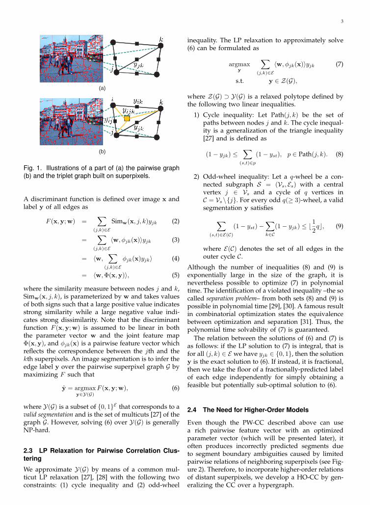
Fig. 1. Illustrations of a part of (a) the pairwise graph(b) and the triplet graph built on superpixels.

A discriminant function is defined over image x andlabel y of all edges as

F (x,y;w) =∑

(j,k)∈E

Simw(x, j, k)yjk (2)

=∑

(j,k)∈E

⟨w, ϕjk(x)⟩yjk (3)

= ⟨w,∑

(j,k)∈E

ϕjk(x)yjk⟩ (4)

= ⟨w,Φ(x,y)⟩, (5)

where the similarity measure between nodes j and k,Simw(x, j, k), is parameterized by w and takes valuesof both signs such that a large positive value indicatesstrong similarity while a large negative value indi-cates strong dissimilarity. Note that the discriminantfunction F (x,y;w) is assumed to be linear in boththe parameter vector w and the joint feature mapΦ(x,y), and ϕjk(x) is a pairwise feature vector whichreflects the correspondence between the jth and thekth superpixels. An image segmentation is to infer theedge label y over the pairwise superpixel graph G bymaximizing F such that

y = argmaxy∈Y(G)

F (x,y;w), (6)

where Y(G) is a subset of {0, 1}E that corresponds to avalid segmentation and is the set of multicuts [27] of thegraph G. However, solving (6) over Y(G) is generallyNP-hard.

2.3 LP Relaxation for Pairwise Correlation Clus-tering

We approximate Y(G) by means of a common mul-ticut LP relaxation [27], [28] with the following twoconstraints: (1) cycle inequality and (2) odd-wheel

inequality. The LP relaxation to approximately solve(6) can be formulated as

argmaxy

∑(j,k)∈E

⟨w, ϕjk(x)⟩yjk (7)

s.t. y ∈ Z(G),

where Z(G) ⊃ Y(G) is a relaxed polytope defined bythe following two linear inequalities.

1) Cycle inequality: Let Path(j, k) be the set ofpaths between nodes j and k. The cycle inequal-ity is a generalization of the triangle inequality[27] and is defined as

(1− yjk) ≤∑

(s,t)∈p

(1− yst), p ∈ Path(j, k). (8)

2) Odd-wheel inequality: Let a q-wheel be a con-nected subgraph S = (Vs, Es) with a centralvertex j ∈ Vs and a cycle of q vertices inC = Vs\{j}. For every odd q(≥ 3)-wheel, a validsegmentation y satisfies∑

(s,t)∈E(C)

(1− yst)−∑k∈C

(1− yjk) ≤ ⌊1

2q⌋, (9)

where E(C) denotes the set of all edges in theouter cycle C.

Although the number of inequalities (8) and (9) isexponentially large in the size of the graph, it isnevertheless possible to optimize (7) in polynomialtime. The identification of a violated inequality –the socalled separation problem– from both sets (8) and (9) ispossible in polynomial time [29], [30]. A famous resultin combinatorial optimization states the equivalencebetween optimization and separation [31]. Thus, thepolynomial time solvability of (7) is guaranteed.

The relation between the solutions of (6) and (7) isas follows: if the LP solution to (7) is integral, that isfor all (j, k) ∈ E we have yjk ∈ {0, 1}, then the solutiony is the exact solution to (6). If instead, it is fractional,then we take the floor of a fractionally-predicted labelof each edge independently for simply obtaining afeasible but potentially sub-optimal solution to (6).

2.4 The Need for Higher-Order Models

Even though the PW-CC described above can usea rich pairwise feature vector with an optimizedparameter vector (which will be presented later), itoften produces incorrectly predicted segments dueto segment boundary ambiguities caused by limitedpairwise relations of neighboring superpixels (see Fig-ure 2). Therefore, to incorporate higher-order relationsof distant superpixels, we develop a HO-CC by gen-eralizing the CC over a hypergraph.

4

(a) (b)

(c) (d)

Fig. 2. Example of segmentation result by PW-CC. (a)Original image. (b) Ground-truth. (c) Superpixels. (d)Segments obtained by PW-CC.

3 HIGHER-ORDER CORRELATION CLUS-TERING

This section describes the proposed HO-CC for imagesegmentation in three steps. In the first step, we definethe hypergraph representation. Second, we generalizethe LP relaxation (7) for hypergraphs. Finally, a featurevector consisting of pairwise and higher-order featurevectors to characterize relationship among superpixelsover a hypergraph is presented.

3.1 Hypergraph

The proposed HO-CC is defined over a hypergraphin which an edge referred to as hyperedge can connectto two or more nodes. For example, as shown inFigure 1.(b), one can introduce binary labels for eachadjacent vertices forming a triplet such that yijk = 1if all vertices in {i, j, k} are in the same cluster;otherwise, yijk = 0. Define a hypergraph HG = (V, E)where V is the set of all nodes (superpixels) and Eis the set of all hyperedges (subsets of V) such that∪

e∈E = V . Here, a hyperedge e has at least twonodes, i.e. |e| ≥ 2. Therefore, the hyperedge set Ecan be divided into two disjoint subsets: pairwiseedge set Ep = {e ∈ E | |e| = 2} and higher-order edge set Eh = {e ∈ E | |e| > 2} such thatEp

∪Eh = E . Note that in the proposed hypergraph

for HO-CC all hyperedges containing just two nodes(∀ep ∈ Ep) are linked between adjacent superpixels.The pairwise superpixel graph is a special hypergraphwhere all hyperedges contain just two (neighboring)superpixels: Ep = E . A binary label ye for a hyperedgee ∈ E is defined such that

ye =

{1, if all nodes in e belong to the same region,0, otherwise.

(10)

3.2 Higher-Order Correlation Clustering over aHypergraph

Similar to the PW-CC, a linear discriminant functionis defined over image x and label y of all hyperedgesas

F (x,y;w)

=∑e∈E

Homw(x, e)ye (11)

=∑e∈E

⟨w, ϕe(x)⟩ye (12)

=∑

ep∈Ep

⟨wp, ϕep(x)⟩yep +∑

eh∈Eh

⟨wh, ϕeh(x)⟩yeh (13)

= ⟨w,Φ(x,y)⟩, (14)

where the homogeneity measure among nodes in e,Homw(x, e), is also the inner product of the parametervector w and the feature vector ϕe(x) and takes valuesof both signs such that a large positive value indicatesstrong homogeneity while a large negative value in-dicates high degree of non-homogeneity. Note thatthe proposed discriminant function for the HO-CCis decomposed into two terms by assigning differentparameter vectors to the pairwise edge set Ep and thehigher-order edge set Eh such that w = [wp;wh]. Thus,in addition to the pairwise similarity between neigh-boring superpixels, the proposed HO-CC considersa broad homogeneous region reflecting higher-orderrelations among superpixels.

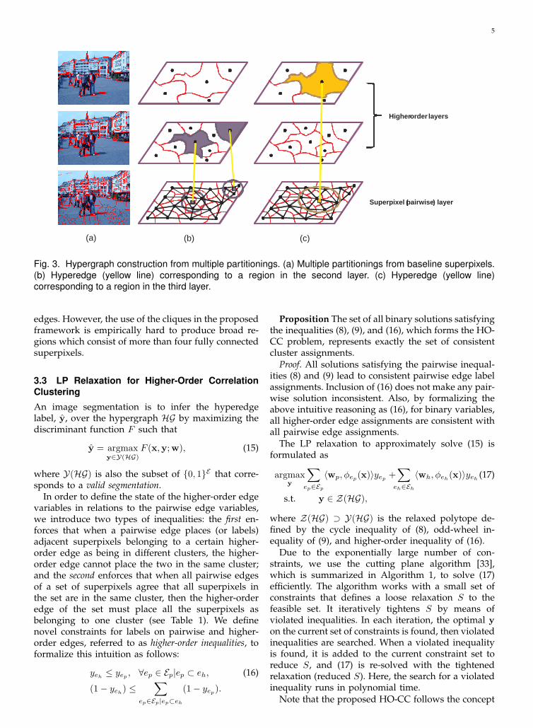
From a given image, a hypergraph is constructed asfollows. First, unsupervised multiple partitionings areobtained by merging not pixels but superpixels withdifferent image quantizations using the ultrametriccontour maps [32]. Then, the obtained regions areused to define hyperedges of the hypergraph. Forexample, in Figure 3, there are three region layers,one superpixel (pairwise) layer and two higher-orderlayers. All edges (black line) in the pairwise super-pixel graph from the first layer are incorporated intothe pairwise edge set Ep. Hyperedges (yellow line)corresponding to regions (groups of superpixels) inthe second and third layers are included in the higher-order edge set Eh. Note that we can further decom-pose the higher-order term in (13) into two terms asso-ciated with the second and third layers, respectively,by assigning different parameter vectors; howeverfor simplicity, this paper aggregates all higher-orderedges from all higher-order layers into a single higher-order edge set assigning the same parameter vector.

The use of unsupervised multiple partitioningsenables to obtain reasonable candidate regions fordefining higher-order edges. Other methods to definehigher-order edges are also possible. For instance,from the baseline pairwise superpixel graph, the fullyconnected subgraphs referred to as cliques whichhave more than two nodes can be obtained, andthese cliques can be associated to the higher-order

5

Superpixel ( pairwise ) layer

Higher - order layers

(a) (b) (c)

Fig. 3. Hypergraph construction from multiple partitionings. (a) Multiple partitionings from baseline superpixels.(b) Hyperedge (yellow line) corresponding to a region in the second layer. (c) Hyperedge (yellow line)corresponding to a region in the third layer.

edges. However, the use of the cliques in the proposedframework is empirically hard to produce broad re-gions which consist of more than four fully connectedsuperpixels.

3.3 LP Relaxation for Higher-Order CorrelationClustering

An image segmentation is to infer the hyperedgelabel, y, over the hypergraph HG by maximizing thediscriminant function F such that

y = argmaxy∈Y(HG)

F (x,y;w), (15)

where Y(HG) is also the subset of {0, 1}E that corre-sponds to a valid segmentation.

In order to define the state of the higher-order edgevariables in relations to the pairwise edge variables,we introduce two types of inequalities: the first en-forces that when a pairwise edge places (or labels)adjacent superpixels belonging to a certain higher-order edge as being in different clusters, the higher-order edge cannot place the two in the same cluster;and the second enforces that when all pairwise edgesof a set of superpixels agree that all superpixels inthe set are in the same cluster, then the higher-orderedge of the set must place all the superpixels asbelonging to one cluster (see Table 1). We definenovel constraints for labels on pairwise and higher-order edges, referred to as higher-order inequalities, toformalize this intuition as follows:

yeh ≤ yep , ∀ep ∈ Ep|ep ⊂ eh, (16)

(1− yeh) ≤∑

ep∈Ep|ep⊂eh

(1− yep).

Proposition The set of all binary solutions satisfyingthe inequalities (8), (9), and (16), which forms the HO-CC problem, represents exactly the set of consistentcluster assignments.

Proof. All solutions satisfying the pairwise inequal-ities (8) and (9) lead to consistent pairwise edge labelassignments. Inclusion of (16) does not make any pair-wise solution inconsistent. Also, by formalizing theabove intuitive reasoning as (16), for binary variables,all higher-order edge assignments are consistent withall pairwise edge assignments.

The LP relaxation to approximately solve (15) isformulated as

argmaxy

∑ep∈Ep

⟨wp, ϕep(x)⟩yep +∑

eh∈Eh

⟨wh, ϕeh(x)⟩yeh (17)

s.t. y ∈ Z(HG),

where Z(HG) ⊃ Y(HG) is the relaxed polytope de-fined by the cycle inequality of (8), odd-wheel in-equality of (9), and higher-order inequality of (16).

Due to the exponentially large number of con-straints, we use the cutting plane algorithm [33],which is summarized in Algorithm 1, to solve (17)efficiently. The algorithm works with a small set ofconstraints that defines a loose relaxation S to thefeasible set. It iteratively tightens S by means ofviolated inequalities. In each iteration, the optimal yon the current set of constraints is found, then violatedinequalities are searched. When a violated inequalityis found, it is added to the current constraint set toreduce S, and (17) is re-solved with the tightenedrelaxation (reduced S). Here, the search for a violatedinequality runs in polynomial time.

Note that the proposed HO-CC follows the concept

6

TABLE 1Label validity for segmentation from the hypergraph (triplet graph) in Figure 1.(b).

yijk 0 0 0 0 0 0 0 0yij 0 0 0 0 1 1 1 1yjk 0 0 1 1 0 0 1 1yik 0 1 0 1 0 1 0 1

Validity valid valid valid invalid valid invalid invalid invalidyijk 1 1 1 1 1 1 1 1yij 0 0 0 0 1 1 1 1yjk 0 0 1 1 0 0 1 1yik 0 1 0 1 0 1 0 1

Validity invalid invalid invalid invalid invalid invalid invalid valid

Algorithm 1 Cutting Plane Algorithm for Inference

Input: w, S ← [0, 1]E

repeatSolve LP relaxation on the current constraint set:

y← argmaxy∈S

∑ep∈Ep

⟨wp, ϕep(x)⟩yep+∑

eh∈Eh

⟨wh, ϕeh(x)⟩yeh

Sviolated ← VIOLATE CYCLE INEQUALITIES (y):check (8)if no violated inequality found thenSviolated ← VIOLATE HIGHER-ORDER IN-EQUALITIES (y): check (16)if no violated inequality found then

Integrality checkif no fractional-predicted label then

breakelseSviolated ← VIOLATE ODD-WHEEL IN-EQUALITIES (y): check (9)

end ifend if

end ifS ← S ∩ Sviolated

until no S has changed

of soft constraints: superpixels belonging to a hyper-edge are not forced but encouraged to merge if ahyperedge is highly homogeneous. This is in linewith recent higher-order models for high-level imageunderstanding [1], [34], [35].

3.4 Feature VectorWe construct a 481-dimensional feature vector ϕe(x) =[ϕep(x);ϕeh(x)] by concatenating several visual cueswith different quantization levels and thresholds.The pairwise feature vector ϕep(x) reflects the cor-respondence between neighboring superpixels, andthe higher-order feature vector ϕeh(x) characterizesa more complex relations among superpixels in abroader region to measure homogeneity. The magni-tude of w determines the importance of each feature,and this importance is task-dependent. Thus, w is

estimated by supervised training described in Section4.

3.4.1 Pairwise feature vectorWe extract several visual cues from a superpixel,including brightness (intensity), color, texture, andshape. Based on these visual cues, we construct a 321-dimensional pairwise feature vector ϕep by concate-nating a color difference feature ϕc, texture differencefeature ϕt, shape/location difference feature ϕs, edgestrength feature ϕe, joint visual word posterior featureϕv , and bias as follows:

ϕep = [ϕcep ;ϕ

tep ;ϕ

sep ;ϕ

eep ;ϕ

vep ; 1]. (18)

• Color difference feature ϕcep : The color difference

feature ϕcep is composed of 26 color distances

between two adjacent superpixels based on RGBand HSV channels. Specifically, we calculate 18earth mover’s distances (EMDs) [36] between twocolor histograms extracted from each superpixelwith various numbers of bins and thresholdsfor ground distance. In addition, six absolutedifferences (one for each color channel) betweenthe means of the two superpixels and two χ2-distances between hue/saturation histograms ofthe two superpixels are concatenated in ϕc

ep .• Texture difference feature ϕt

ep : The 64-dimensional texture difference feature ϕt

ep iscomposed of 15 absolute differences (one foreach texture-response) between the means of twosuperpixels using 15 Leung-Malik (LM) filterbanks [37] and one χ2-distance and 48 EMDs(from various numbers of bins and thresholdsfor ground distance) between texture histogramsof the two superpixels.

• Shape/location difference feature ϕsep : The 5-

dimensional shape/location difference featureϕsep is composed of two absolute differences be-

tween the normalized (x/y) center positions ofthe two superpixels, the ratio of the size of thesmaller superpixel to that of the larger super-pixel, the percentage of boundary with respectto the smaller superpixel, and the straightness ofboundary [4].

7

• Edge strength feature ϕeep : The 15-dimensional

edge strength feature ϕeep is a 1-of-15 coding of the

quantized edge strength proposed by Arbelaez etal. [32].

• Joint visual word posterior feature ϕvep : The 210-

dimensional joint visual word posterior featureϕvep is defined as the vector holding the joint

visual word posteriors for a pair of neighboringsuperpixels using 20 visual words [38] as follows.First, a 52-dimensional raw feature vector xj

based on color, texture, location, and shape fea-tures described in [4] is extracted from the jthsuperpixel. Then, the visual word posterior distri-bution P (vi|xj) is computed using the GaussianRBF kernel where vi denotes the ith visual word.Let Vjk(x) be a 20-by-20 matrix whose elementsare the joint visual word posteriors betweennodes j and k defined such that

Vjk(x)

=

P (v1|xj)P (v1|xk) · · · P (v1|xj)P (v20|xk)P (v2|xj)P (v1|xk) · · · P (v2|xj)P (v20|xk)

.... . .

...P (v20|xj)P (v1|xk)· · ·P (v20|xj)P (v20|xk)

. (19)

The joint visual word posterior feature betweennodes j and k, ϕv

jk(x), is defined as

ϕvjk(x) = vec

(Vjk(x)

)+ vec

(V Tjk(x)

), (20)

where vec(V ) be the 210(= 20 × 21/2)-dimensional vector whose elements are from theupper triangular part of V .This joint visual word posterior feature couldovercome the weakness of class-agnostic featuresand incorporate the contextual information.

3.4.2 Higher-order feature vectorWe construct a 160-dimensional higher-order featurevector ϕeh by concatenating the variance feature ϕva

eh,

edge strength feature ϕeeh

, template matching featureϕtmeh

and bias as follows:

ϕeh = [ϕvaeh;ϕe

eh;ϕtm

eh; 1]. (21)

• Variance feature ϕvaeh

: The 44-dimensional vari-ance feature is a generalized version of thecolor/texture difference feature used in the pair-wise graph. We calculate 14 color variancesamong superpixels in a hyperedge based onthe average RGB and HSV values and thehue/saturation histograms with 8 bins. In addi-tion, 30 texture variances from 15 mean textureresponses and texture response histogram with15 bins are incorporated into the variance featurevector.

• Edge strength feature ϕeeh

: The 15-dimensionaledge strength feature ϕe

ehis a ℓ1-normalized his-

togram of the quantized edge strengths of neigh-boring superpixels in eh.

• Template matching feature ϕtmeh

: The 44-dimensional color/texture features and 5-dimensional shape/location features of all (task-specific ground truth) regions in the trainingimages are clustered using k-means with k = 100to obtain 100 representative templates of distinctregions. The 100-dimensional template matchingfeature vector is composed of the matchingscores between a region defined by hyperedgeand these templates using the Gaussian RBFkernel.

Note that in each feature vector, the bias (=1)is augmented in order to obtain a proper similar-ity/homogeneity measure which can either be posi-tive or negative.

4 STRUCTURAL LEARNING

The proposed discriminant function is defined overthe superpixel graph, and therefore, the ground-truthsegmentation needs to be transformed to the ground-truth edge labels in the superpixel graph. For this, wefirst assign a single dominant segment label to eachsuperpixel by majority voting over the superpixel’sconstituent pixels and then obtain the ground-truthedge labels according to whether dominant labels ofsuperpixels in a hyperedge are equal or not.

Using this ground-truth edge labels of the trainingdata, we use the S-SVM to estimate the parametervector for task-specific CC. We use the cutting planealgorithm with LP relaxation (17) for loss-augmentedinference to solve the optimization problem of theS-SVM, since fast convergence and high robustnessof the cutting plane algorithm in handling a largenumber of margin constraints are well-known [14].

4.1 Structured Support Vector MachineGiven N training samples {(xn,yn)}Nn=1 where yn

is the ground-truth edge labels for the nth trainingimage xn, the S-SVM [14] optimizes w by minimizinga quadratic objective function subject to a set of linearmargin constraints:

minw,ξ

1

2∥w∥2 + C

N∑n=1

ξn (22)

s.t. ∀n,y ∈ Z(HG),⟨w,∆Φ(xn,y)⟩ ≥ ∆(yn,y)− ξn,

∀n, ξn ≥ 0,

where ∆Φ(xn,y) = Φ(xn,yn)−Φ(xn,y), and C > 0 isa constant that controls the trade-off between marginmaximization and training error minimization. In theS-SVM, the margin is scaled with a loss ∆(yn,y),which is the difference measure between predictiony and ground-truth label yn of the nth image. The S-SVM offers good generalization ability as well as theflexibility to choose any loss function [14].

8

Algorithm 2 Cutting Plane Algorithm for S-SVMChoose: w0, C, R, ϵSn ← ø, ∀n, w← w0, ξ ← 0repeat

for n = 1, ..., N doPerform the loss-augmented inference by LPrelaxation:

yn = argmaxy∈Z(HG)

(⟨w,Φ(xn,y)⟩+∆(yn,y)

)if −⟨w, δΦ(xn, yn)⟩+∆(yn, yn) > ξn + ϵ thenSn ← Sn ∪ {yn}

end ifend forSolve the restricted problem of (22) on the currentset of constraints:

(w∗, ξ∗) = argminw′,ξ′

1

2∥w′∥2 + C

N∑n=1

ξ′n

s.t. ⟨w′, δΦ(xn,y)⟩ ≥ ∆(yn,y)− ξ′n, ∀n,y ∈ Sn,

ξ′n ≥ 0, ∀n

Update: w← w∗, ξ ← ξ∗

until no Sn has changed

4.2 Cutting Plane AlgorithmThe exponentially large number of margin constraintsand the intractability of the loss-augmented inferenceproblem make it difficult to solve the constrainedoptimization problem of (22). Therefore, we apply thecutting plane algorithm [14] to approximately solvethe constrained optimization problem. The cuttingplane algorithm is summarized in Algorithm 2. Ineach iteration, the most violated constraint for eachtraining sample is approximately found by perform-ing the loss-augmented inference using the LP re-laxation. The computational cost for inference canbe greatly reduced when a decomposable loss suchas the Hamming loss is used. When a loss functioncan be decomposed in the same manner as the jointfeature map, it can be added to each edge score inthe inference. It can then be checked whether theconstraint found tightens the feasible set of (22) ornot, and when it does, then the parameter vector wand ξ are updated by solving the restricted problemof (22) on the current set of active constraints thatincludes it. The theoretical convergence and robust-ness of the cutting plane algorithm was studied byTsochantaridis et al. [14]. The LP relaxations for loss-augmented inferences are considered to be well suitedto structured learning [39]–[41].

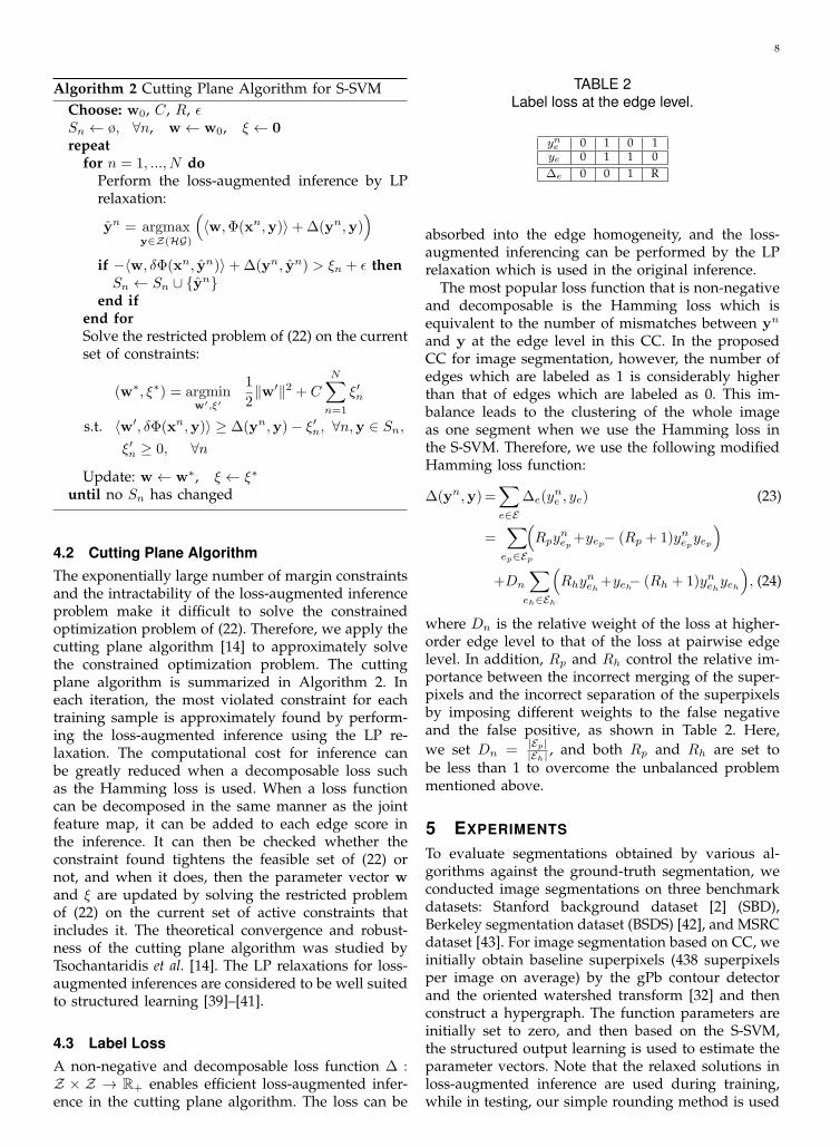
4.3 Label LossA non-negative and decomposable loss function ∆ :Z × Z → R+ enables efficient loss-augmented infer-ence in the cutting plane algorithm. The loss can be

TABLE 2Label loss at the edge level.

yne 0 1 0 1ye 0 1 1 0∆e 0 0 1 R

absorbed into the edge homogeneity, and the loss-augmented inferencing can be performed by the LPrelaxation which is used in the original inference.

The most popular loss function that is non-negativeand decomposable is the Hamming loss which isequivalent to the number of mismatches between yn

and y at the edge level in this CC. In the proposedCC for image segmentation, however, the number ofedges which are labeled as 1 is considerably higherthan that of edges which are labeled as 0. This im-balance leads to the clustering of the whole imageas one segment when we use the Hamming loss inthe S-SVM. Therefore, we use the following modifiedHamming loss function:

∆(yn,y)=∑e∈E

∆e(yne , ye) (23)

=∑

ep∈Ep

(Rpy

nep+yep− (Rp + 1)ynepyep

)+Dn

∑eh∈Eh

(Rhy

neh+yeh− (Rh + 1)ynehyeh

), (24)

where Dn is the relative weight of the loss at higher-order edge level to that of the loss at pairwise edgelevel. In addition, Rp and Rh control the relative im-portance between the incorrect merging of the super-pixels and the incorrect separation of the superpixelsby imposing different weights to the false negativeand the false positive, as shown in Table 2. Here,we set Dn =

|Ep||Eh| , and both Rp and Rh are set to

be less than 1 to overcome the unbalanced problemmentioned above.

5 EXPERIMENTS

To evaluate segmentations obtained by various al-gorithms against the ground-truth segmentation, weconducted image segmentations on three benchmarkdatasets: Stanford background dataset [2] (SBD),Berkeley segmentation dataset (BSDS) [42], and MSRCdataset [43]. For image segmentation based on CC, weinitially obtain baseline superpixels (438 superpixelsper image on average) by the gPb contour detectorand the oriented watershed transform [32] and thenconstruct a hypergraph. The function parameters areinitially set to zero, and then based on the S-SVM,the structured output learning is used to estimate theparameter vectors. Note that the relaxed solutions inloss-augmented inference are used during training,while in testing, our simple rounding method is used

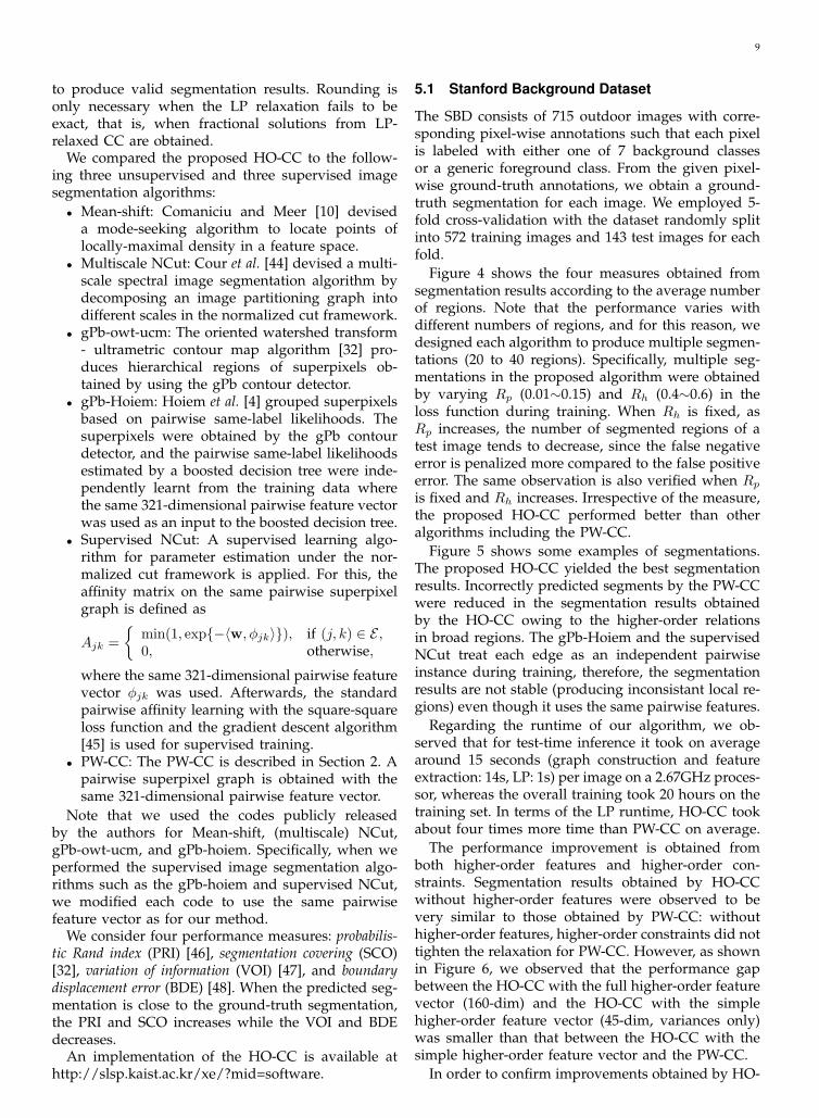
9

to produce valid segmentation results. Rounding isonly necessary when the LP relaxation fails to beexact, that is, when fractional solutions from LP-relaxed CC are obtained.

We compared the proposed HO-CC to the follow-ing three unsupervised and three supervised imagesegmentation algorithms:

• Mean-shift: Comaniciu and Meer [10] deviseda mode-seeking algorithm to locate points oflocally-maximal density in a feature space.

• Multiscale NCut: Cour et al. [44] devised a multi-scale spectral image segmentation algorithm bydecomposing an image partitioning graph intodifferent scales in the normalized cut framework.

• gPb-owt-ucm: The oriented watershed transform- ultrametric contour map algorithm [32] pro-duces hierarchical regions of superpixels ob-tained by using the gPb contour detector.

• gPb-Hoiem: Hoiem et al. [4] grouped superpixelsbased on pairwise same-label likelihoods. Thesuperpixels were obtained by the gPb contourdetector, and the pairwise same-label likelihoodsestimated by a boosted decision tree were inde-pendently learnt from the training data wherethe same 321-dimensional pairwise feature vectorwas used as an input to the boosted decision tree.

• Supervised NCut: A supervised learning algo-rithm for parameter estimation under the nor-malized cut framework is applied. For this, theaffinity matrix on the same pairwise superpixelgraph is defined as

Ajk =

{min(1, exp{−⟨w, ϕjk⟩}), if (j, k) ∈ E ,0, otherwise,

where the same 321-dimensional pairwise featurevector ϕjk was used. Afterwards, the standardpairwise affinity learning with the square-squareloss function and the gradient descent algorithm[45] is used for supervised training.

• PW-CC: The PW-CC is described in Section 2. Apairwise superpixel graph is obtained with thesame 321-dimensional pairwise feature vector.

Note that we used the codes publicly releasedby the authors for Mean-shift, (multiscale) NCut,gPb-owt-ucm, and gPb-hoiem. Specifically, when weperformed the supervised image segmentation algo-rithms such as the gPb-hoiem and supervised NCut,we modified each code to use the same pairwisefeature vector as for our method.

We consider four performance measures: probabilis-tic Rand index (PRI) [46], segmentation covering (SCO)[32], variation of information (VOI) [47], and boundarydisplacement error (BDE) [48]. When the predicted seg-mentation is close to the ground-truth segmentation,the PRI and SCO increases while the VOI and BDEdecreases.

An implementation of the HO-CC is available athttp://slsp.kaist.ac.kr/xe/?mid=software.

5.1 Stanford Background Dataset

The SBD consists of 715 outdoor images with corre-sponding pixel-wise annotations such that each pixelis labeled with either one of 7 background classesor a generic foreground class. From the given pixel-wise ground-truth annotations, we obtain a ground-truth segmentation for each image. We employed 5-fold cross-validation with the dataset randomly splitinto 572 training images and 143 test images for eachfold.

Figure 4 shows the four measures obtained fromsegmentation results according to the average numberof regions. Note that the performance varies withdifferent numbers of regions, and for this reason, wedesigned each algorithm to produce multiple segmen-tations (20 to 40 regions). Specifically, multiple seg-mentations in the proposed algorithm were obtainedby varying Rp (0.01∼0.15) and Rh (0.4∼0.6) in theloss function during training. When Rh is fixed, asRp increases, the number of segmented regions of atest image tends to decrease, since the false negativeerror is penalized more compared to the false positiveerror. The same observation is also verified when Rp

is fixed and Rh increases. Irrespective of the measure,the proposed HO-CC performed better than otheralgorithms including the PW-CC.

Figure 5 shows some examples of segmentations.The proposed HO-CC yielded the best segmentationresults. Incorrectly predicted segments by the PW-CCwere reduced in the segmentation results obtainedby the HO-CC owing to the higher-order relationsin broad regions. The gPb-Hoiem and the supervisedNCut treat each edge as an independent pairwiseinstance during training, therefore, the segmentationresults are not stable (producing inconsistant local re-gions) even though it uses the same pairwise features.

Regarding the runtime of our algorithm, we ob-served that for test-time inference it took on averagearound 15 seconds (graph construction and featureextraction: 14s, LP: 1s) per image on a 2.67GHz proces-sor, whereas the overall training took 20 hours on thetraining set. In terms of the LP runtime, HO-CC tookabout four times more time than PW-CC on average.

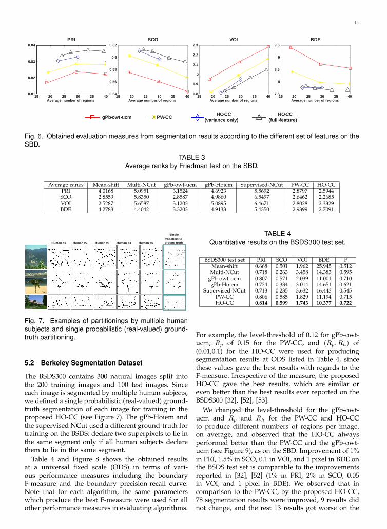
The performance improvement is obtained fromboth higher-order features and higher-order con-straints. Segmentation results obtained by HO-CCwithout higher-order features were observed to bevery similar to those obtained by PW-CC: withouthigher-order features, higher-order constraints did nottighten the relaxation for PW-CC. However, as shownin Figure 6, we observed that the performance gapbetween the HO-CC with the full higher-order featurevector (160-dim) and the HO-CC with the simplehigher-order feature vector (45-dim, variances only)was smaller than that between the HO-CC with thesimple higher-order feature vector and the PW-CC.

In order to confirm improvements obtained by HO-

10

20 25 30 35 40 0.74

0.76

0.78

0.8

0.82

0.84

Average number of regions

PRI

20 25 30 35 40

0.3

0.4

0.5

0.6

Average number of regions

SCO

Mean - Shift Multi - NCut gPb - owt - ucm

gPb - Hoiem Supervised - NCut PW - CC HO - CC

20 25 30 35 40

2

2.5

3

Average number of regions

VOI

20 25 30 35 40

8

9

10

11

12

Average number of regions

BDE

Fig. 4. Obtained evaluation measures from segmentation results on the SBD.

Ground - truth Multi - NCut gPb - Hoiem gPb - owt - ucm Original image Mean - Shift Supervised -

NCut PW - CC HO - CC

Fig. 5. Results of image segmentation on the SBD.

CC are statistically significant, we performed statis-tical hypothesis tests for each performance measure.The Friedman test [49], [50] was used to evaluatethe null-hypothesis that all the algorithms performequally well. Table 3 shows the obtained averageranks. Under the null-hypothesis, all average ranksshould be equal. However, as shown in Table 3, theranks are different, and the null-hypothesis is rejectedfor all the four measures. This is also verified bythe obtained p-values which are numerically equal tozeros for all the four measures. Furthermore, we per-formed a post-hoc test, called Nemenyi test [50], [51]for pairwise comparison of algorithms, testing for thenull-hypothesis of pairwise equal performance. The

Nemenyi test is based on the difference of the averageperformance ranks achieved by the algorithms; if thedifference between two ranks exceeds a critical value,the null-hypothesis is refuted. As a result, at the levelα = 0.05, with the PRI and BDE measures, the HO-CC is statistically significantly superior to all otheralgorithms except PW-CC, with the VOI measures,the HO-CC is statistically significantly superior toall other algorithms except Mean-shift, and with theSCO measures, the HO-CC is statistically significantlysuperior to all other algorithms.

11

15 20 25 30 35 40 0.81

0.82

0.83

0.84

Average number of regions

PRI

15 20 25 30 35 40 1.8

1.9

2

2.1

2.2

2.3

Average number of regions

VOI

15 20 25 30 35 40 0.54

0.56

0.58

0.6

0.62

Average number of regions

SCO

15 20 25 30 35 40 7.5

8

8.5

9

9.5

Average number of regions

BDE

gPb - owt - ucm PW - CC HO - CC

(full - feature) HO - CC

(variance only)

Fig. 6. Obtained evaluation measures from segmentation results according to the different set of features on theSBD.

TABLE 3Average ranks by Friedman test on the SBD.

Average ranks Mean-shift Multi-NCut gPb-owt-ucm gPb-Hoiem Supervised-NCut PW-CC HO-CCPRI 4.0168 5.0951 3.1524 4.6923 5.5692 2.8797 2.5944SCO 2.8559 5.8350 2.8587 4.9860 6.5497 2.6462 2.2685VOI 2.5287 5.6587 3.1203 5.0895 6.4671 2.8028 2.3329BDE 4.2783 4.4042 3.3203 4.9133 5.4350 2.9399 2.7091

Human #1 Human #2 Human #3 Human #4 Human #5

Single p robabilistic ground truth

Fig. 7. Examples of partitionings by multiple humansubjects and single probabilistic (real-valued) ground-truth partitioning.

5.2 Berkeley Segmentation Dataset

The BSDS300 contains 300 natural images split intothe 200 training images and 100 test images. Sinceeach image is segmented by multiple human subjects,we defined a single probabilistic (real-valued) ground-truth segmentation of each image for training in theproposed HO-CC (see Figure 7). The gPb-Hoiem andthe supervised NCut used a different ground-truth fortraining on the BSDS: declare two superpixels to lie inthe same segment only if all human subjects declarethem to lie in the same segment.

Table 4 and Figure 8 shows the obtained resultsat a universal fixed scale (ODS) in terms of vari-ous performance measures including the boundaryF-measure and the boundary precision-recall curve.Note that for each algorithm, the same parameterswhich produce the best F-measure were used for allother performance measures in evaluating algorithms.

TABLE 4Quantitative results on the BSDS300 test set.

BSDS300 test set PRI SCO VOI BDE FMean-shift 0.668 0.501 1.962 25.945 0.512Multi-NCut 0.718 0.263 3.458 14.383 0.595

gPb-owt-ucm 0.807 0.571 2.039 11.001 0.710gPb-Hoiem 0.724 0.334 3.014 14.651 0.621

Supervised-NCut 0.713 0.235 3.632 16.443 0.545PW-CC 0.806 0.585 1.829 11.194 0.715HO-CC 0.814 0.599 1.743 10.377 0.722

For example, the level-threshold of 0.12 for gPb-owt-ucm, Rp of 0.15 for the PW-CC, and (Rp, Rh) of(0.01,0.1) for the HO-CC were used for producingsegmentation results at ODS listed in Table 4, sincethese values gave the best results with regards to theF-measure. Irrespective of the measure, the proposedHO-CC gave the best results, which are similar oreven better than the best results ever reported on theBSDS300 [32], [52], [53].

We changed the level-threshold for the gPb-owt-ucm and Rp and Rh for the PW-CC and HO-CCto produce different numbers of regions per image,on average, and observed that the HO-CC alwaysperformed better than the PW-CC and the gPb-owt-ucm (see Figure 9), as on the SBD. Improvement of 1%in PRI, 1.5% in SCO, 0.1 in VOI, and 1 pixel in BDE onthe BSDS test set is comparable to the improvementsreported in [32], [52] (1% in PRI, 2% in SCO, 0.05in VOI, and 1 pixel in BDE). We observed that incomparison to the PW-CC, by the proposed HO-CC,78 segmentation results were improved, 9 results didnot change, and the rest 13 results got worse on the

12

0.4 0.5 0.6 0.7 0.8 0.9 10.4

0.5

0.6

0.7

0.8

0.9

1

Recall

Pre

cisi

on

Mean−ShiftMulti−NcutgPb−owt−ucmgPb−HoiemSupervised−NCutPW−CCHO−CC

Fig. 8. Boundary precision-recall curve on theBSDS300 test set.

15 20 25 30 35 40 0.78

0.8

0.82

0.84

0.86

Average number of regions

PRI

15 20 25 30 35 40 1.6

1.7

1.8

1.9

2

Average number of regions

VOI

15 20 25 30 35 40

0.58

0.6

0.62

0.64

Average number of regions

SCO

15 20 25 30 35 40 10

10.5

11

11.5

12

12.5

Average number of regions

BDE

gPb - owt - ucm PW - CC HO - CC

Fig. 9. Obtained evaluation measures from segmen-tation results of gPb-owt-ucm, PW-CC, and HO-CC onthe BSDS300 test set according to the average numberof regions.

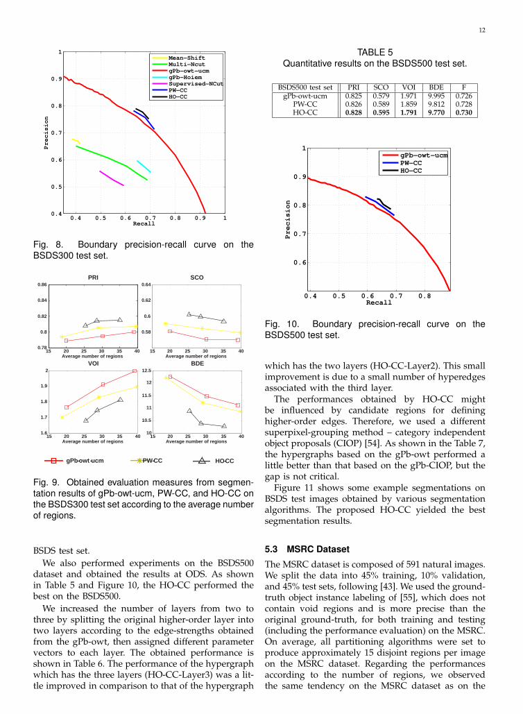
BSDS test set.We also performed experiments on the BSDS500

dataset and obtained the results at ODS. As shownin Table 5 and Figure 10, the HO-CC performed thebest on the BSDS500.

We increased the number of layers from two tothree by splitting the original higher-order layer intotwo layers according to the edge-strengths obtainedfrom the gPb-owt, then assigned different parametervectors to each layer. The obtained performance isshown in Table 6. The performance of the hypergraphwhich has the three layers (HO-CC-Layer3) was a lit-tle improved in comparison to that of the hypergraph

TABLE 5Quantitative results on the BSDS500 test set.

BSDS500 test set PRI SCO VOI BDE FgPb-owt-ucm 0.825 0.579 1.971 9.995 0.726

PW-CC 0.826 0.589 1.859 9.812 0.728HO-CC 0.828 0.595 1.791 9.770 0.730

0.4 0.5 0.6 0.7 0.8

0.6

0.7

0.8

0.9

1

Recall

Pre

cisi

on

gPb−owt−ucmPW−CCHO−CC

Fig. 10. Boundary precision-recall curve on theBSDS500 test set.

which has the two layers (HO-CC-Layer2). This smallimprovement is due to a small number of hyperedgesassociated with the third layer.

The performances obtained by HO-CC mightbe influenced by candidate regions for defininghigher-order edges. Therefore, we used a differentsuperpixel-grouping method – category independentobject proposals (CIOP) [54]. As shown in the Table 7,the hypergraphs based on the gPb-owt performed alittle better than that based on the gPb-CIOP, but thegap is not critical.

Figure 11 shows some example segmentations onBSDS test images obtained by various segmentationalgorithms. The proposed HO-CC yielded the bestsegmentation results.

5.3 MSRC Dataset

The MSRC dataset is composed of 591 natural images.We split the data into 45% training, 10% validation,and 45% test sets, following [43]. We used the ground-truth object instance labeling of [55], which does notcontain void regions and is more precise than theoriginal ground-truth, for both training and testing(including the performance evaluation) on the MSRC.On average, all partitioning algorithms were set toproduce approximately 15 disjoint regions per imageon the MSRC dataset. Regarding the performancesaccording to the number of regions, we observedthe same tendency on the MSRC dataset as on the

13

Original Image Multi - NCut gPb - Hoiem gPb - owt - ucm PW - CC Mean - Shift Supervised -

NCut HO - CC

Fig. 11. Results of image segmentation on the BSDS test set.

TABLE 6Quantitative results on the BSDS500 test set

according to the number of layers.

BSDS500 test set PRI SCO VOI BDE FHO-CC-Layer2 0.828 0.595 1.791 9.770 0.730HO-CC-Layer3 0.829 0.599 1.786 9.764 0.730

TABLE 7Quantitative results on the BSDS500 test setaccording to different superpixel-groupings for

hypergraph construction.

BSDS500 test set PRI SCO VOI BDE FHO-CC-gPb-owt 0.828 0.595 1.791 9.770 0.730

HO-CC-gPb-CIOP 0.826 0.592 1.801 9.797 0.728

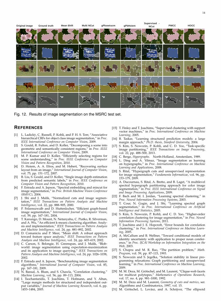
BSDS dataset. As shown in Table 8 and Figure 12, theproposed HO-CC gave the best results on the test set.

We also trained on the MSRC dataset and testedon the BSDS dataset. This decreases the performanceover training and testing on the BSDS dataset. Thisobservation is also true in the reverse direction, i.e.when training on the BSDS dataset and testing onthe MSRC dataset. Overall, this suggests that the twodatasets have different statistics, and the proposedframework allows the segmentation to be tuned tothe particular dataset at hand.

TABLE 8Quantitative results on the MSRC test set.

MSRC test set PRI SCO VOI BDEMean-shift 0.734 0.606 1.649 13.944Multi-NCut 0.628 0.341 2.765 11.941

gPb-owt-ucm 0.779 0.628 1.675 9.800gPb-Hoiem 0.614 0.353 2.847 13.533

Supervised-NCut 0.601 0.287 3.101 13.498PW-CC 0.773 0.632 1.648 9.194HO-CC 0.784 0.648 1.594 9.040

6 CONCLUSION

This paper proposed the HO-CC over a hypergraphto merge superpixels into homogeneous regions. TheLP relaxation was used to approximately solve theinference problem over a hypergraph where a richfeature vector was defined based on several visualcues involving higher-order relations among super-pixels. The S-SVM was used for supervised trainingof parameters in CC, and the cutting plane algo-rithm with LP-relaxed inference was applied to solvethe optimization problem of S-SVM. Experimentalresults showed that the proposed HO-CC outper-formed other image segmentation algorithms on var-ious datasets. The proposed framework is applicableto a variety of other tasks.

14

Ground - truth Multi - NCut gPb - Hoiem gPb - owt - ucm Original image Mean - Shift Supervised -

NCut PW - CC HO - CC

Fig. 12. Results of image segmentation on the MSRC test set.

REFERENCES

[1] L. Ladicky, C. Russell, P. Kohli, and P. H. S. Torr, “Associativehierarchical CRFs for object class image segmentation,” in Proc.IEEE International Conference on Computer Vision, 2009.

[2] S. Gould, R. Fulton, and D. Koller, “Decomposing a scene intogeometric and semantically consistent regions,” in Proc. IEEEInternational Conference on Computer Vision, 2009.

[3] M. P. Kumar and D. Koller, “Efficiently selecting regions forscene understanding,” in Proc. IEEE Conference on ComputerVision and Pattern Recognition, 2010.

[4] D. Hoiem, A. A. Efros, and M. Hebert, “Recovering surfacelayout from an image,” International Journal of Computer Vision,vol. 75, pp. 151–172, 2007.

[5] B. Liu, S. Gould, and D. Koller, “Single image depth estimationfrom predicted semantic labels,” in Proc. IEEE Conference onComputer Vision and Pattern Recognition, 2010.

[6] F. Estrada and A. Jepson, “Spectral embedding and mincut forimage segmentation,” in Proc. British Machine Vision Conference(BMVC), 2004.

[7] J. Shi and J. Malik, “Normalized cuts and image segmen-tation,” IEEE Transactions on Pattern Analysis and MachineIntelligence, vol. 22, pp. 888–905, 2000.

[8] P. Felzenszwalb and D. Huttenlocher, “Efficient graph-basedimage segmentation,” International Journal of Computer Vision,vol. 59, pp. 167–181, 2004.

[9] T. Kanungo, D. Mount, N. Netanyahu, C. Piatko, R. Silverman,and A. Wu, “An efficient k-means clustering algorithm: Analy-sis and implementation,” IEEE Transactions on Pattern Analysisand Machine Intelligence, vol. 24, pp. 881–892, 2002.

[10] D. Comaniciu and P. Meer, “Mean shift: A robust approachtoward feature space analysis,” IEEE Transactions on PatternAnalysis and Machine Intelligence, vol. 24, pp. 603–619, 2002.

[11] C. Carson, S. Belongie, H. Greenspan, and J. Malik, “Blob-world: image segmentation using expectation-maximizationand its application to image querying,” IEEE Transactions onPattern Analysis and Machine Intelligence, vol. 24, pp. 1026–1038,2002.

[12] F. Estrada and A. Jepson, “Benchmarking image segmentationalgorithms,” International Journal of Computer Vision, vol. 85,pp. 167–181, 2009.

[13] N. Bansal, A. Blum, and S. Chawla, “Correlation clustering,”Machine Learning, vol. 56, pp. 89–113, 2004.

[14] I. Tsochantaridis, T. Joachims, T. Hofmann, and Y. Altun,“Large margin methods for structured and independent out-put variables,” Journal of Machine Learning Research, vol. 6, pp.1453–1484, 2005.

[15] T. Finley and T. Joachims, “Supervised clustering with supportvector machines,” in Proc. International Conference on MachineLearning, 2005.

[16] B. Taskar, “Learning structured prediction models: a largemargin approach,” Ph.D. thesis, Stanford University, 2004.

[17] S. Kim, S. Nowozin, P. Kohli, and C. D. Yoo, “Task-specificimage partitioning,” IEEE Transactions on Image Processing,vol. 22, pp. 488–500, 2013.

[18] C. Berge, Hypergraphs. North-Holland, Amsterdam, 1989.[19] L. Ding and A. Yilmaz, “Image segmentation as learning

on hypergraphs,” in Proc. International Conference on MachineLearning and Applications, 2008.

[20] S. Rital, “Hypergraph cuts and unsupervised representationfor image segmentation,” Fundamenta Informaticae, vol. 96, pp.153–179, 2009.

[21] A. Ducournau, S. Rital, A. Bretto, and B. Laget, “A multilevelspectral hypergraph partitioning approach for color imagesegmentation,” in Proc. IEEE International Conference on Signaland Image Processing Applications, 2009.

[22] F. Bach and M. I. Jordan, “Learning spectral clustering,” inProc. Neural Information Processing Systems, 2003.

[23] T. Cour, N. Gogin, and J. Shi, “Learning spectral graphsegmentation,” in Proc. International Conference on ArtificialIntelligence and Statistics, 2005.

[24] S. Kim, S. Nowozin, P. Kohli, and C. D. Yoo, “Higher-ordercorrelation clustering for image segmentation,” in Proc. NeuralInformation Processing Systems, 2011.

[25] T. Joachims and J. E. Hopcroft, “Error bounds for correlationclustering,” in Proc. International Conference on Machine Learn-ing, 2005.

[26] A. McCallum and B. Wellner, “Toward conditional models ofidentity uncertainty with application to proper noun corefer-ence,” in Proc. IJCAI Workshop on Information Integration on theWeb, 2003.

[27] S. Chopra and M. R. Rao, “The partition problem,” Math.Program, vol. 59, pp. 87–115, 1993.

[28] S. Nowozin and S. Jegelka, “Solution stability in linear pro-gramming relaxations: Graph partitioning and unsupervisedlearning,” in Proc. International Conference on Machine Learning,2009.

[29] M. M. Deza, M. Grotschel, and M. Laurent, “Clique-web facetsfor multicut polytopes,” Mathematics of Operations Research,vol. 17, no. 4, pp. 981–1000, 1992.

[30] M. M. Deza and M. Laurent, Geometry of cuts and metrics, ser.Algorithms and Combinatorics, 1997, vol. 15.

[31] M. Grotschel, L. Lovasz, and A. Schrijver, “The ellipsoid

15

method and its consequences in combinatorial optimization,”Combinatorica, vol. 1, pp. 169–197, 1981.

[32] P. Arbelaez, M. Maire, C. Fowlkes, and J. Malik, “Contourdetection and hierarchical image segmentation,” IEEE Trans-actions on Pattern Analysis and Machine Intelligence, vol. 33, pp.898–916, 2011.

[33] L. Wolsey, Integer programming. John Wiley, 1998.[34] P. Kohli, L. Ladicky, and P. H. S. Torr, “Robust higher order

potentials for enforcing label consistency,” International Journalof Computer Vision, vol. 82, pp. 302–324, 2009.

[35] L. Ding and A. Yilmaz, “Interactive image segmentation usingprobabilistic hypergraphs,” Pattern Recognition, vol. 43, pp.1863–1873, 2010.

[36] O. Pele and M. Werman, “Fast and robust earth mover’sdistances,” in Proc. IEEE International Conference on ComputerVision, 2009.

[37] T. Leung and J. Malik, “Representing and recognizing the vi-sual appearance of materials using three-dimensional textons,”International Journal of Computer Vision, vol. 43, pp. 29–44, 2001.

[38] D. Batra, R. Sukthankar, and T. Chen, “Learning class-specificaffinities for image labelling,” in Proc. IEEE Conference onComputer Vision and Pattern Recognition, 2008.

[39] T. Finley and T. Joachims, “Training structural SVMs whenexact inference is intractable,” in Proc. International Conferenceon Machine Learning, 2008.

[40] A. Kulesza and F. Pereira, “Structured learning with approxi-mate inference,” in Proc. Neural Information Processing Systems,2007.

[41] A. F. T. Martins, N. A. Smith, and E. P. Xing, “Polyhedral outerapproximations with application to natural language parsing,”in Proc. International Conference on Machine Learning, 2009.

[42] C. Fowlkes, D. Martin, and J. Malik, The Berke-ley Segmentation Dataset and Benchmark (BSDB),http://www.cs.berkeley.edu/projects/vision/grouping/.

[43] J. Shotton, J. Winn, C. Rother, and A. Criminisi, “Textonboost:joint appearence, shape and context modeling for multi-classobject recognition and segmentation,” in Proc. European Con-ference on Computer Vision (ECCV), 2006.

[44] T. Cour, F. Benezit, and J. Shi, “Spectral segmentation withmultiscale graph decomposition,” in Proc. IEEE Conference onComputer Vision and Pattern Recognition, 2005.

[45] S. Turaga, K. Briggman, M. Helmstaedter, W. Denk, andH. Seung, “Maximin affinity learning of image segmentation,”in Proc. Neural Information Processing Systems, 2009.

[46] W. M. Rand, “Objective criteria for the evaluation of clusteringmethods,” Journal of the American Statistical Association, vol. 66,pp. 846–850, 1971.

[47] M. Meila, “Computing clusterings: An axiomatic view,” inProc. International Conference on Machine Learning, 2005.

[48] J. Freixenet, X. Munoz, D. Raba, J. Marti, and X. Cufi, “Yetanother survey on image segmentation: Region and bound-ary information integration,” in Proc. European Conference onComputer Vision (ECCV), 2002.

[49] M. Friedman, “A comparison of alternative tests of signifi-cance for the problem of m rankings,” Annals of MathematicalStatistics, vol. 11, pp. 86–92, 1940.

[50] J. Demsar, “Statistical comparisons of classifiers over multipledata sets,” Journal of Machine Learning Research, vol. 7, pp. 1–30,2006.

[51] P. B. Nemenyi, “Distribution-free multiple comparisons,”Ph.D. thesis, Princeton University, 1963.

[52] T. Kim, K. Lee, and S. Lee, “Learning full pairwise affinities forspectral segmentation,” in Proc. IEEE Conference on ComputerVision and Pattern Recognition, 2010.

[53] S. R. Rao, H. Mobahi, A. Y. Yang, S. S. Sastry, and Y. Ma, “Nat-ural image segmentation with adaptive texture and bound-ary encoding,” in Proc. Asian Conference on Computer Vision(ACCV), 2009.

[54] I. Endres and D. Hoiem, “Category independent object propos-als,” in Proc. European Conference on Computer Vision (ECCV),2010.

[55] T. Malisiewicz and A. A. Efros, “Improving spatial support forobjects via multiple segmentations,” in Proc. British MachineVision Conference (BMVC), 2007.

Sungwoong Kim (S’07-M’12) received theB.S. and Ph.D. degrees in electrical engi-neering from Korea Advanced Institute ofScience and Technology (KAIST), Daejeon,Korea, in 2004 and 2011, respectively. Since2012 he is with Qualcomm Research Koreawhere he is a senior engineer. His researchinterests include machine learning for multi-media signal processing, discriminative train-ing, and graphical modeling.

Chang D. Yoo (S’92-M’96-SM’11) receivedthe B.S. degree in Engineering and AppliedScience from California Institute of Technol-ogy in 1986, the M.S. degree in Electrical En-gineering from Cornell University in 1988 andthe Ph.D. degree in Electrical Engineeringfrom Massachusetts Institute of Technologyin 1996. From January 1997 to March 1999he worked at Korea Telecom as a SeniorResearcher. He joined the Department ofElectrical Engineering at Korea Advanced

Institute of Science and Technology in April 1999. From March 2005to March 2006, he was with Research Laboratory of Electronics atMIT. His current research interests are in the application of machinelearning and digital signal processing in multimedia.

Sebastian Nowozin is a researcher in theMachine Learning and Perception group atMicrosoft Research Cambridge. He receivedhis Master of Engineering degree from theShanghai Jiaotong University (SJTU) and hisdiploma degree in computer science withdistinction from the Technical University ofBerlin in 2006. He received his PhD degreesumma cum laude in 2009 for his thesison learning with structured data in computervision, completed at the Max Planck Institute

for Biological Cybernetics, Tubingen and the Technical Universityof Berlin. His research interest is at the intersection of computervision and machine learning. He regularly serves as PC-memberand reviewer for machine learning (NIPS, ICML, AISTATS, UAI,ECML, JMLR) and computer vision (CVPR, ICCV, ECCV, PAMI,IJCV) conferences and journals.

Pushmeet Kohli is a senior research scien-tist in the Machine Learning and Perceptiongroup at Microsoft Research Cambridge, andis a part of the Association for ComputingMachinery’s (ACM) Distinguished SpeakerProgram. His research has appeared in con-ferences and journals in Computer Vision,Machine Learning, Robotics, AI, ComputerGraphics, and HCI conferences. He has wonbest paper awards in ICVGIP 2006, 2010,ECCV 2010 and ISMAR 2011. His PhD the-

sis, titled ”Minimizing Dynamic and Higher Order Energy Functionsusing Graph Cuts”, was the winner of the British Machine VisionAssociation’s ”Sullivan Doctoral Thesis Award”, and was a runner-up for the British Computer Society’s ”Distinguished DissertationAward”. Dr. Kohli’s research has also been featured in popular mediaoutlets such as Forbes, The Economic Times, New Scientist and MITTechnology Review.