
Edge Detection Selim Aksoy Department of Computer Engineering Bilkent University [email protected].
Upload
julie-fordCategory
view
214download
0
CS 484, Spring 2008 ©2008, Selim Aksoy 2
Image segmentation

CS 484, Spring 2008 ©2008, Selim Aksoy 3
Image segmentation
CS 484, Spring 2008 ©2008, Selim Aksoy 4
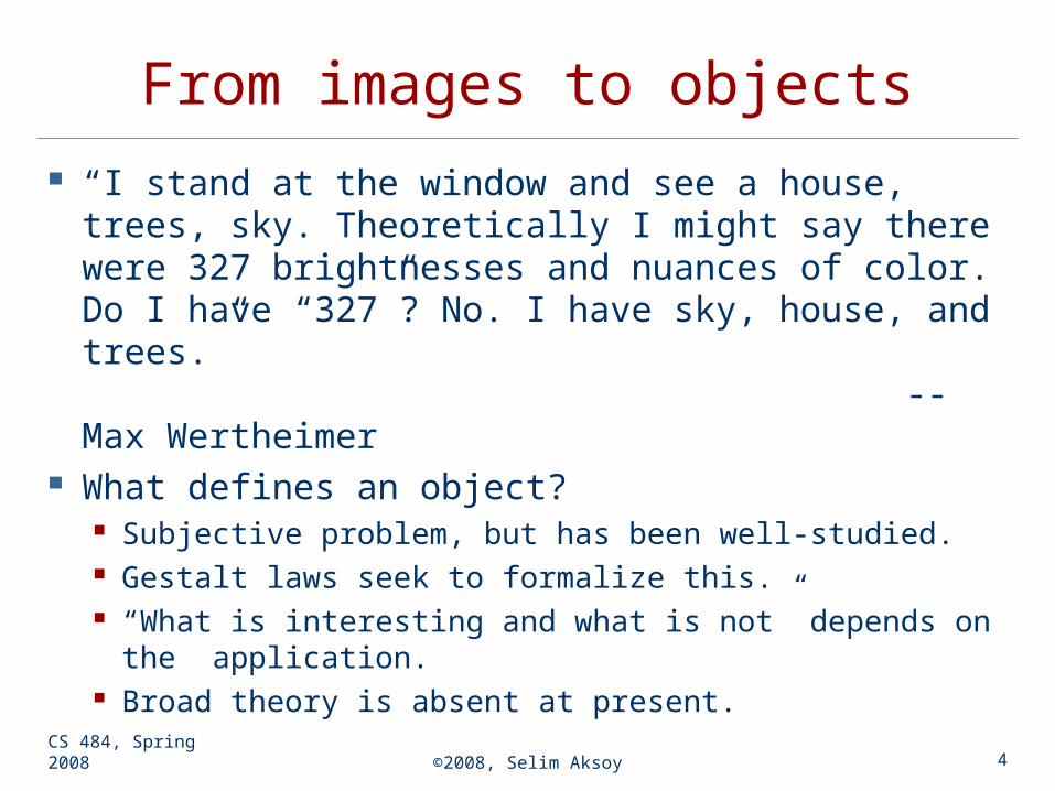
From images to objects
“I stand at the window and see a house, trees, sky. Theoretically I might say there were 327 brightnesses and nuances of color. Do I have “327”? No. I have sky, house, and trees.” -- Max Wertheimer
What defines an object? Subjective problem, but has been well-studied. Gestalt laws seek to formalize this. “What is interesting and what is not” depends on
the application. Broad theory is absent at present.

CS 484, Spring 2008 ©2008, Selim Aksoy 5
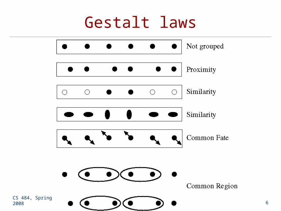
Gestalt laws A series of factors affect whether elements should
be grouped together. Proximity: tokens that are nearby tend to be grouped. Similarity: similar tokens tend to be grouped together. Common fate: tokens that have coherent motion tend to
be grouped together. Common region: tokens that lie inside the same closed
region tend to be grouped together. Parallelism: parallel curves or tokens tend to be grouped
together. Closure: tokens or curves that tend to lead to closed
curves tend to be grouped together. Symmetry: curves that lead to symmetric groups are
grouped together. Continuity: tokens that lead to “continuous” curves tend to
be grouped. Familiar configuration: tokens that, when grouped, lead to
a familiar object, tend to be grouped together.
CS 484, Spring 2008 ©2008, Selim Aksoy 6
Gestalt laws

CS 484, Spring 2008 ©2008, Selim Aksoy 7
Gestalt laws
CS 484, Spring 2008 ©2008, Selim Aksoy 8
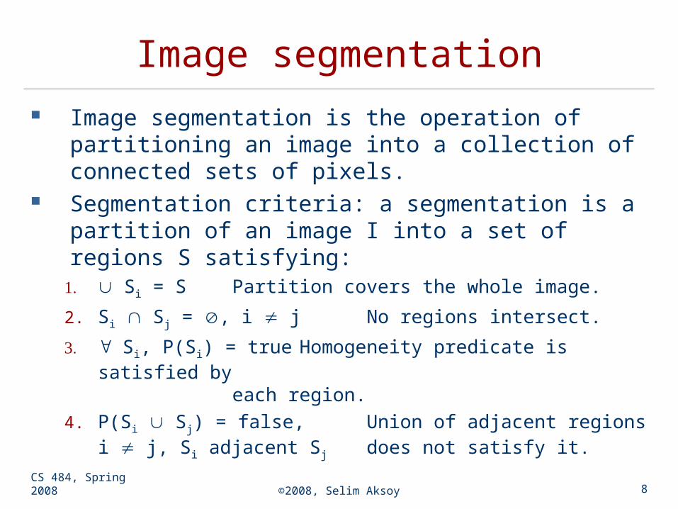
Image segmentation Image segmentation is the operation of
partitioning an image into a collection of connected sets of pixels.
Segmentation criteria: a segmentation is a partition of an image I into a set of regions S satisfying:1. Si = S Partition covers the whole image.
2. Si Sj = , i j No regions intersect.
3. Si, P(Si) = true Homogeneity predicate is satisfied by
each region.4. P(Si Sj) = false, Union of adjacent regions
i j, Si adjacent Sj does not satisfy it.

CS 484, Spring 2008 ©2008, Selim Aksoy 9
Image segmentation So, all we have to do is to define and
implement the similarity predicate. But, what do we want to be similar in each region? Is there any property that will cause the regions to
be meaningful objects? Example approaches:
Histogram-based Clustering-based Region growing Split-and-merge Morphological Graph-based

CS 484, Spring 2008 ©2008, Selim Aksoy 10
Histogram-based segmentation How many “orange” pixels are
in this image? This type of question can be answered
by looking at the histogram.

CS 484, Spring 2008 ©2008, Selim Aksoy 11
Histogram-based segmentation
How many modes are there? Solve this by reducing the number of colors to K
and mapping each pixel to the closest color. Here’s what it looks like if we use two colors.

CS 484, Spring 2008 ©2008, Selim Aksoy 12
Clustering-based segmentation
How to choose the representative colors? This is a clustering problem!
K-means algorithm can be used for clustering.
CS 484, Spring 2008 ©2008, Selim Aksoy 13
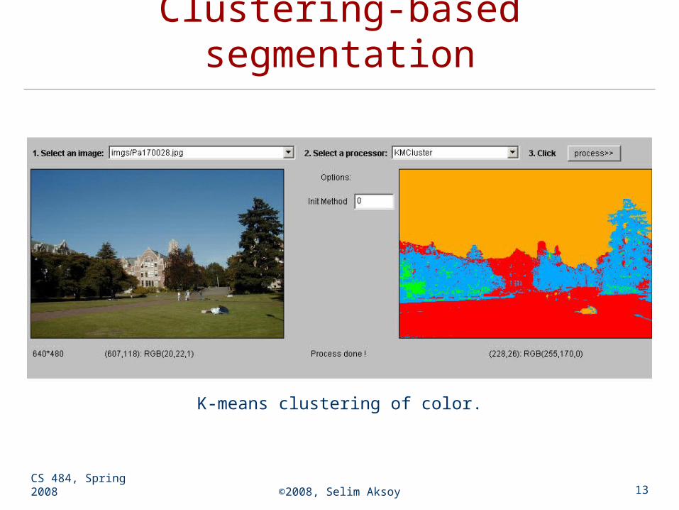
Clustering-based segmentation
K-means clustering of color.

CS 484, Spring 2008 ©2008, Selim Aksoy 14
Clustering-based segmentation
K-means clustering of color.

CS 484, Spring 2008 ©2008, Selim Aksoy 15
Clustering-based segmentation
Clustering can also be used with other features (e.g., texture) in addition to color.
Original Images
Color Regions
Texture Regions

CS 484, Spring 2008 ©2008, Selim Aksoy 16
Clustering-based segmentation
K-means variants: Different ways to initialize the means. Different stopping criteria. Dynamic methods for determining the right
number of clusters (K) for a given image. Problem: histogram-based and clustering-
based segmentation using color/texture/etc can produce messy regions. (Why?)
How can these be fixed?

CS 484, Spring 2008 ©2008, Selim Aksoy 17
Clustering-based segmentation
Expectation-Maximization (EM) algorithm can be used as a probabilistic clustering method where each cluster is modeled using a Gaussian.
The clusters are updated iteratively by computing the parameters of the Gaussians.
Example from the UC Berkeley’s Blobworld system.
CS 484, Spring 2008 ©2008, Selim Aksoy 18
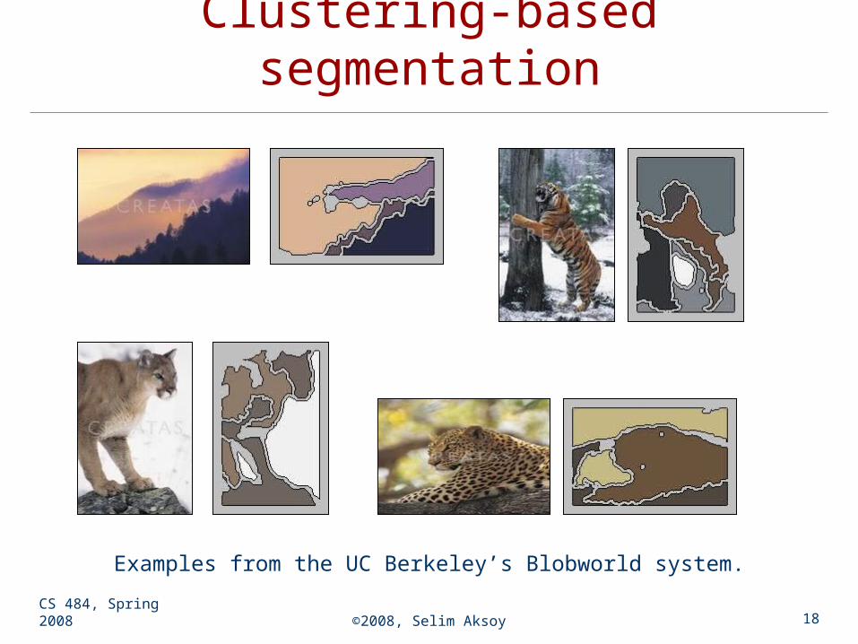
Clustering-based segmentation
Examples from the UC Berkeley’s Blobworld system.

CS 484, Spring 2008 ©2008, Selim Aksoy 19
Region growing Region growing techniques start with one
pixel of a potential region and try to grow it by adding adjacent pixels till the pixels being compared are too dissimilar.
The first pixel selected can be just the first unlabeled pixel in the image or a set of seed pixels can be chosen from the image.
Usually a statistical test is used to decide which pixels can be added to a region. Region is a population with similar statistics. Use statistical test to see if neighbor on border
fits into the region population.
CS 484, Spring 2008 ©2008, Selim Aksoy 20
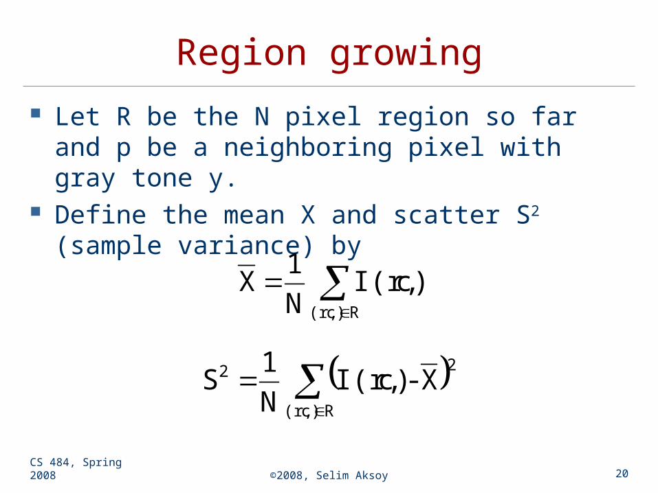
Region growing
Let R be the N pixel region so far and p be a neighboring pixel with gray tone y.
Define the mean X and scatter S2 (sample variance) by
Rc)(r,
c)I(r,N1
X
2
Rc)(r,
2 X-c)I(r,N1
S

CS 484, Spring 2008 ©2008, Selim Aksoy 21
Region growing
The T statistic is defined by
It has a TN-1 distribution if all the pixels in R and the test pixel p are independent and identically distributed Gaussians (i.i.d. assumption).
1/2
22 /S)X(p1)(N
1)N(NT

CS 484, Spring 2008 ©2008, Selim Aksoy 22
Region growing
For the T distribution, statistical tables give us the probability Pr(T ≤ t) for a given degrees of freedom and a confidence level. From this, pick a suitable threshold t.
If the computed T ≤ t for desired confidence level, add p to region R and update the mean and scatter using p.
If T is too high, the value p is not likely to have arisen from the population of pixels in R. Start a new region.
CS 484, Spring 2008 ©2008, Selim Aksoy 23
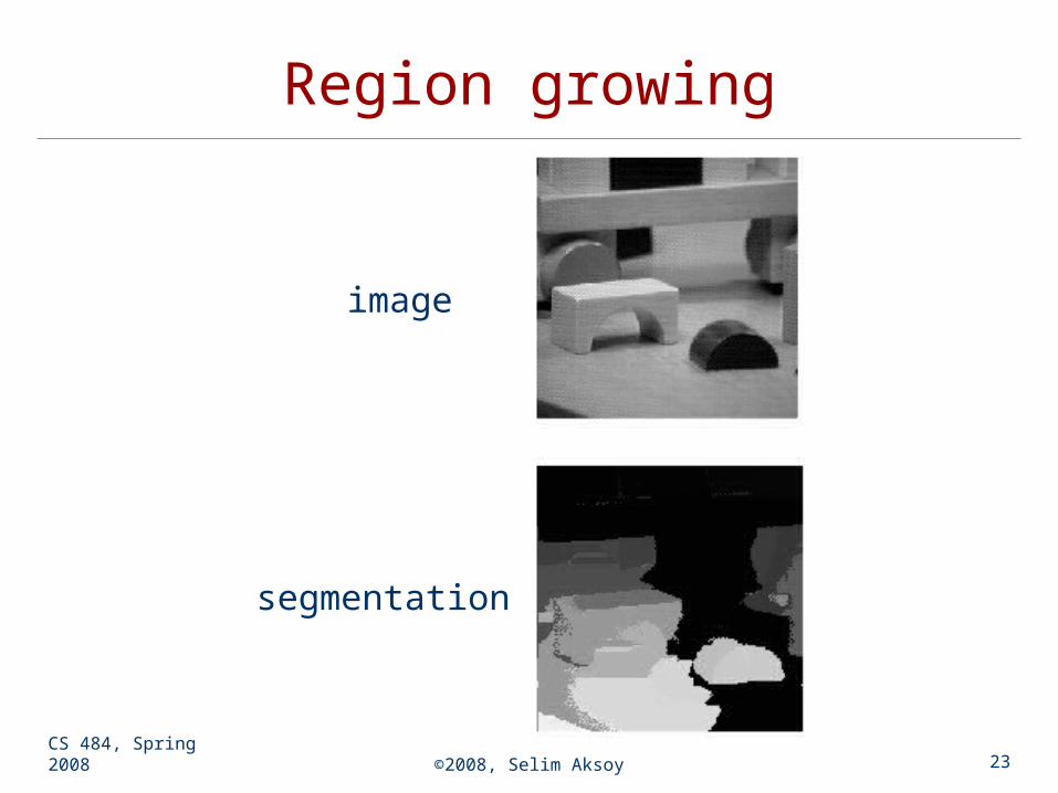
Region growing
image
segmentation

CS 484, Spring 2008 ©2008, Selim Aksoy 24
Split-and-merge
1. Start with the whole image.2. If the variance is too high, break into
quadrants.3. Merge any adjacent regions that are
similar enough.4. Repeat steps 2 and 3, iteratively until no
more splitting or merging occur.
Idea: goodResults: blocky

CS 484, Spring 2008 ©2008, Selim Aksoy 25
Split-and-merge

CS 484, Spring 2008 ©2008, Selim Aksoy 26
Split-and-merge
CS 484, Spring 2008 ©2008, Selim Aksoy 27
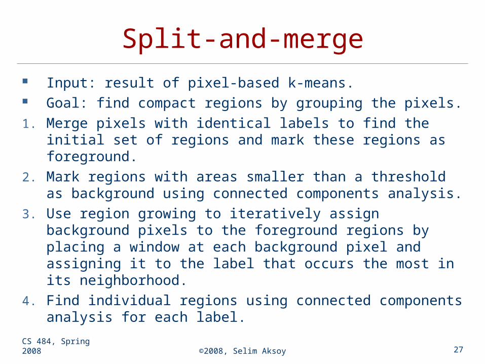
Split-and-merge Input: result of pixel-based k-means. Goal: find compact regions by grouping the pixels.1. Merge pixels with identical labels to find the initial
set of regions and mark these regions as foreground.
2. Mark regions with areas smaller than a threshold as background using connected components analysis.
3. Use region growing to iteratively assign background pixels to the foreground regions by placing a window at each background pixel and assigning it to the label that occurs the most in its neighborhood.
4. Find individual regions using connected components analysis for each label.
CS 484, Spring 2008 ©2008, Selim Aksoy 28
Split-and-merge
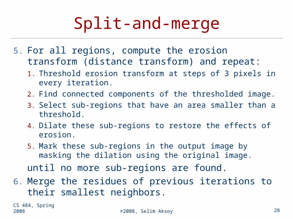
5. For all regions, compute the erosion transform (distance transform) and repeat:1. Threshold erosion transform at steps of 3 pixels in every
iteration.2. Find connected components of the thresholded image.3. Select sub-regions that have an area smaller than a
threshold.4. Dilate these sub-regions to restore the effects of erosion.5. Mark these sub-regions in the output image by masking
the dilation using the original image.
until no more sub-regions are found.6. Merge the residues of previous iterations to their
smallest neighbors.

CS 484, Spring 2008 ©2008, Selim Aksoy 29
Split-and-merge
A large connected region formed by
merging pixels labeled as residential after
classification.
A satellite image. More compact sub-regions after the split-and-merge procedure.
CS 484, Spring 2008 ©2008, Selim Aksoy 30
Watershed segmentation
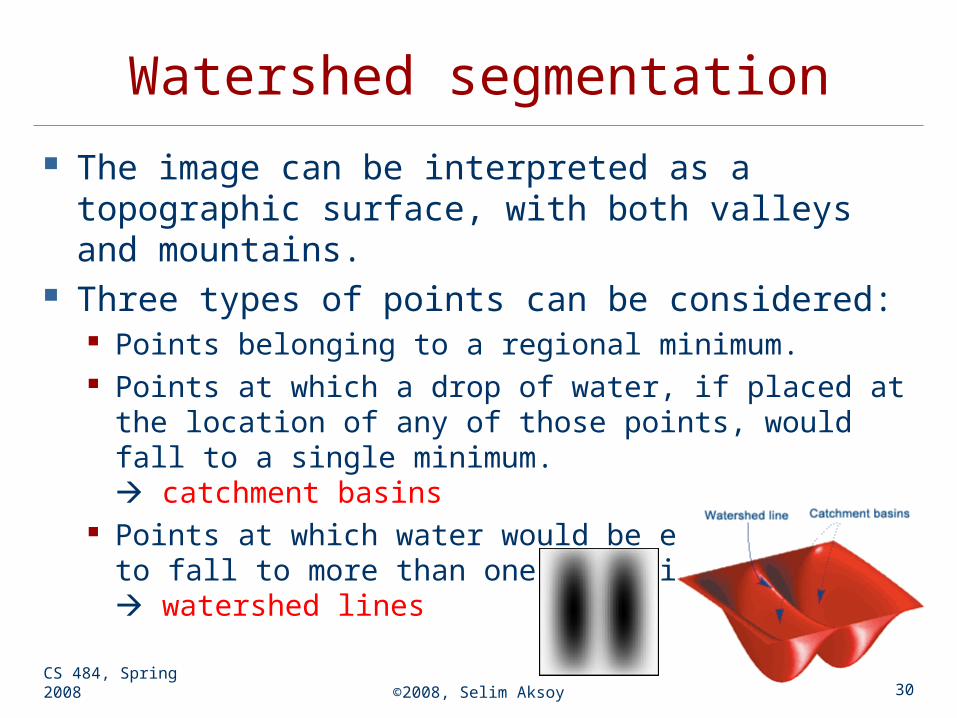
The image can be interpreted as a topographic surface, with both valleys and mountains.
Three types of points can be considered: Points belonging to a regional minimum. Points at which a drop of water, if placed at the
location of any of those points, would fall to a single minimum. catchment basins
Points at which water would be equally likely to fall to more than one such minimum. watershed lines

CS 484, Spring 2008 ©2008, Selim Aksoy 31
Watershed segmentation
Assume that there is a hole in each minima and the surface is immersed into a lake.
The water will enter through the holes at the minima and flood the surface.
To avoid the water coming from two different minima to meet, a dam is build whenever there would be a merge of the water.
Finally, the only thing visible of the surface would be the dams. These dam walls are called the watershed lines.

CS 484, Spring 2008 ©2008, Selim Aksoy 32
Watershed segmentation
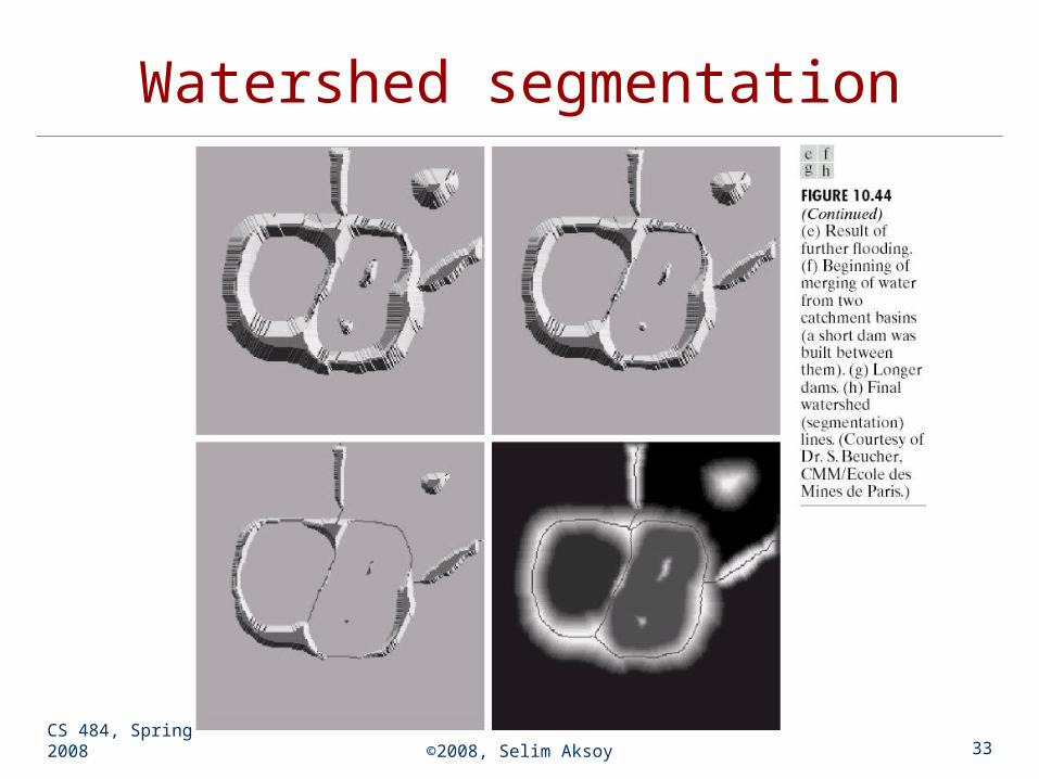
CS 484, Spring 2008 ©2008, Selim Aksoy 33
Watershed segmentation

CS 484, Spring 2008 ©2008, Selim Aksoy 34
Watershed segmentation

CS 484, Spring 2008 ©2008, Selim Aksoy 35
Watershed segmentation The key behind using the watershed transform
for segmentation is this: change your image into another image whose catchment basins are the objects you want to identify.
Examples: Distance transform can be used with binary images
where the catchment basins correspond to the foreground components of interest.
Gradient can be used with grayscale images where the catchment basins should theoretically correspond to the homogeneous grey level regions of the image.

CS 484, Spring 2008 ©2008, Selim Aksoy 36
Watershed segmentationbw Distance transform of ~bw Watershed transform of D
Binary image. Distance transform of the complement of the binary image.
Watershed transform after complementing the distance transform, and forcing pixels that do not belong to the objects to be at –Inf.

CS 484, Spring 2008 ©2008, Selim Aksoy 37
Watershed segmentation

CS 484, Spring 2008 ©2008, Selim Aksoy 38
Watershed segmentation

CS 484, Spring 2008 ©2008, Selim Aksoy 39
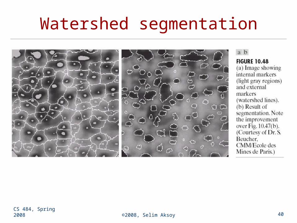
Watershed segmentation
A major enhancement of the watershed transformation consists in flooding the topographic surface from a
previously defined set of markers.
CS 484, Spring 2008 ©2008, Selim Aksoy 40
Watershed segmentation

CS 484, Spring 2008 ©2008, Selim Aksoy 41
Graph-based segmentation
An image is represented by a graph whose nodes are pixels or small groups of pixels.
The goal is to partition the nodes into disjoint sets so that the similarity within each set is high and across different sets is low.

CS 484, Spring 2008 ©2008, Selim Aksoy 42
Graph-based segmentation
Let G = (V,E) be a graph. Each edge (u,v) has a weight w(u,v) that represents the similarity between u and v.
Graph G can be broken into 2 disjoint graphs with node sets A and B by removing edges that connect these sets.
Let cut(A,B) = w(u,v).
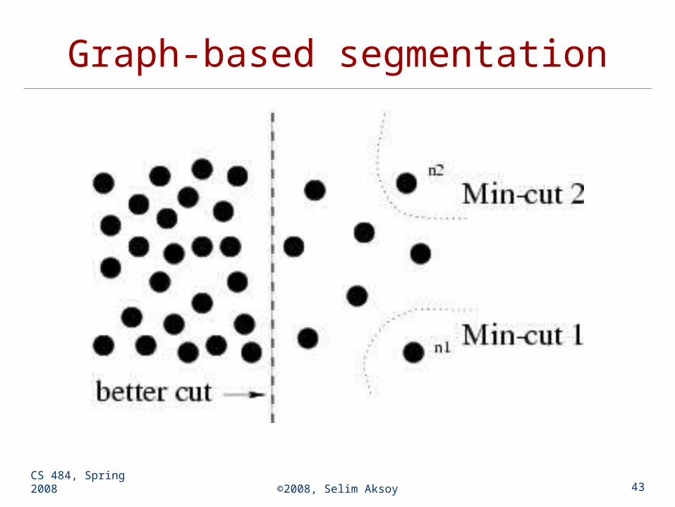
One way to segment G is to find the minimal cut.
uA, vB
CS 484, Spring 2008 ©2008, Selim Aksoy 43
Graph-based segmentation

CS 484, Spring 2008 ©2008, Selim Aksoy 44
Graph-based segmentation
Minimal cut favors cutting off small node groups, so Shi and Malik proposed the normalized cut. cut(A,B) cut(A,B)Ncut(A,B) = --------------- + --------------- assoc(A,V) assoc(B,V)
assoc(A,V) = w(u,t) uA, tV
How much is A connectedto the graph as a whole
Normalizedcut

CS 484, Spring 2008 ©2008, Selim Aksoy 45
Graph-based segmentation
2
2 2
2 2
41 3
2
2 2
3
2
2
2
1
3 3Ncut(A,B) = ------- + ------ 21 16
A B

CS 484, Spring 2008 ©2008, Selim Aksoy 46
Graph-based segmentation
Shi and Malik turned graph cuts into an eigenvector/eigenvalue problem.
Set up a weighted graph G=(V,E). V is the set of (N) pixels. E is a set of weighted edges (weight wij gives the
similarity between nodes i and j). Length N vector d: di is the sum of the weights
from node i to all other nodes. N x N matrix D: D is a diagonal matrix with d on
its diagonal. N x N symmetric matrix W: Wij = wij.

CS 484, Spring 2008 ©2008, Selim Aksoy 47
Graph-based segmentation Let x be a characteristic vector of a set A of nodes.
xi = 1 if node i is in a set A xi = -1 otherwise
Let y be a continuous approximation to x
Solve the system of equations(D – W) y = D y
for the eigenvectors y and eigenvalues . Use the eigenvector y with second smallest
eigenvalue to bipartition the graph (y x A). If further subdivision is merited, repeat recursively.

CS 484, Spring 2008 ©2008, Selim Aksoy 48
Graph-based segmentation
Edge weights w(i,j) can be defined by
w(i,j) = e *
where X(i) is the spatial location of node I F(i) is the feature vector for node I
which can be intensity, color, texture, motion… The formula is set up so that w(i,j) is 0 for
nodes that are too far apart.
||F(i)-F(j)||2 / I2 e if ||X(i)-X(j)||2 < r
0 otherwise
||X(i)-X(j)||2 / X2

CS 484, Spring 2008 ©2008, Selim Aksoy 49
Graph-based segmentation