Image Segmentation for Animal Images using Finite … · Image Segmentation for Animal Images using...

© 2014. K. Srinivasa Rao, P. Chandra Sekhar & P. Srinivasa Rao. This is a research/review paper, distributed under the terms of the Creative Commons Attribution-Noncommercial 3.0 Unported License http://creativecommons.org/licenses/by-nc/3.0/), permitting all non-commercial use, distribution, and reproduction inany medium, provided the original work is properly cited.

Global Journal of Computer Science and Technology: F Graphics & Vision Volume 14 Issue 3 Version 1.0 Year 2014 Type: Double Blind Peer Reviewed International Research Journal Publisher: Global Journals Inc. (USA) Online ISSN: 0975-4172 & Print ISSN: 0975-4350

Image Segmentation for Animal Images using Finite Mixture of Pearson type VI Distribution

By K. Srinivasa Rao, P. Chandra Sekhar & P. Srinivasa Rao GITAM University, India

Abstract- Image Segmentation is one of the significant tool for analyzing images, the feature vector of the images are different for different types of images. In remote sensing, Environmental ecological systems, forest studies, conservation of rare animals, the animal images are more important. In this paper we developed and analyze an image segmentation algorithm using mixture of Pearson Type VI Distribution. The Pearsonian Type VI Distribution will characterize the image regions of animal images. The appropriateness Pearsonian Type VI distribution for the pixel intensities of image region in animal images is carried by fitting Pearsonian Type VI Distribution to set of animal images taken from Berkeley image data set. The image segmentation algorithm is developed using EM algorithm for estimating the parameters of the model and maximum likelihood for image component under Bayesian framework. For fast convergence of EM algorithm the initial estimates of the model parameters are obtained by dividing the whole image into K image regions using K-means and Hierarchical clustering algorithm and utilizing the moment method of estimates. The performance of proposed algorithm is studied by conducting an experiment with set of animal images and computing image quality metrics such as PRI, GCE and VOI.

Keywords: EM algorithm, image segmentation, performance measures, type VI pearsonian.

GJCST-F Classification :

ImageSegmentationforAnimalImagesusingFiniteMxtureofPearsontypeVIDistribution

Strictly as per the compliance and regulations of:

I.4.0


K. Srinivasa Rao α, P. Chandra Sekhar σ & P. Srinivasa Rao ρ

Abstract- Image Segmentation is one of the significant tool for analyzing images, the feature vector of the images are different for different types of images. In remote sensing, Environmental ecological systems, forest studies, conservation of rare animals, the animal images are more important. In this paper we developed and analyze an image segmentation algorithm using mixture of Pearson Type VI Distribution. The Pearsonian Type VI Distribution will characterize the image regions of animal images. The appropriateness Pearsonian Type VI distribution for the pixel intensities of image region in animal images is carried by fitting Pearsonian Type VI Distribution to set of animal images taken from Berkeley image data set. The image segmentation algorithm is developed using EM algorithm for estimating the parameters of the model and maximum likelihood for image component under Bayesian framework. For fast convergence of EM algorithm the initial estimates of the model parameters are obtained by dividing the whole image into K image regions using K-means and Hierarchical clustering algorithm and utilizing the moment method of estimates. The performance of proposed algorithm is studied by conducting an experiment with set of animal images and computing image quality metrics such as PRI, GCE and VOI. A comparative study of developed image segmentation by Gaussian Mixture model and found the proposed algorithm performed better for animal images due to asymmetrically distributed nature of pixel intensities in the image regions. Keywords: EM algorithm, image segmentation, performance measures, type VI pearsonian.

I. Introduction

n image processing and retrievals image analysis plays a dominant role. The major task in image analysis is extracting useful information using

features of the image. Generally image analysis techniques broadly grouping into groups namely (1) Structural methods (2) Statistical methods Raj Kumar et al (2011), among these two groups statistical methods are much popular. In Statistical methods one of the prime considerations is dividing whole image into different image regions using probability distributions. This type of method is usually referred as image

Author

α:

Department of Statistics, Andhra University, Visakhapatnam. e-mail: [email protected]

Author

σ:

Department of IT, GITAM University, Visakhapatnam.

e-mail: [email protected]

Author

ρ:

Department of CS&SE, Andhra University, Visakhapatnam.

e-mail: [email protected]

Pal

N.

R.

(1993), Cheng

et

al

(2001),

Srinivasa

et

al

(2007), Srinivas Y et al (2010), Prasad Reddy et al (2007) have reviewed the image segmentation methods. There is no unique image segmentation method available for analyzing all images. The image segmentation is basically dependent on type of images. The image broadly categorized into four types of categories . They are (1) Images on Earth (2) images of Humans and animals (3) images on sky (4) images on Water and (5) images of Nature. Among these categories the images of Human beings and Animals are in different in nature and features are associated with these images are different from others in some statistical sense. These images are Skewed in nature. Hence the image segmentation methods based on Gaussian mixture model given by Cheng et al (2001), Yamazaki T. et al (1998), Zhang Z.H et al (2003), Lie T. et al (1993) may not suit well. Even the methods given by Sesha sayee et al (2011), Srinivasa et al (2011) are also may not suit since these methods also focus on symmetry of the pixel intensities in the image region. Hence to have suitable and more appropriate image segmentation methods for animals, an image segmentation method using a mixture of Pearsonian Type VI Distribution is developed and analyzed. Here it is assumed that whole image is characterized by a mixture of Pearsonian Type VI probability model. The Pearsonian Type VI Distribution is skewed in nature having long upper tails. This distribution also includes several distributions as particular case. From the Berkeley image data set collected over animal images. It is evident that the pixel intensities of these images are well categorized by mixture of Pearsonian Type VI Distribution. The model parameters are estimated by updated equations of EM algorithm. The initial values of the model parameters of EM Algorithm are carried using Histograms of the whole image and K-means and Hierarchical clustering Algorithm and moment method of estimates. The image segmentation algorithm is developed through Maximum Likelihood component under Bayesian frame. The performance of image segmentation algorithm is skewed using image quality metrics and ground truth values. The comparative study of proposed algorithm with that of Gaussian Mixture Model is also carried.

I

Segmentation.Much work has been reported in literature

regarding image segmentation methods. Pal S.K and

© 2014 Global Journals Inc. (US)

Globa

l Jo

urna

l of C

ompu

ter Sc

ienc

e an

d Te

chno

logy

Volum

e XIV

Issu

e III

Versio

n I

1

(DDDD DDDD

)Year

2014

F

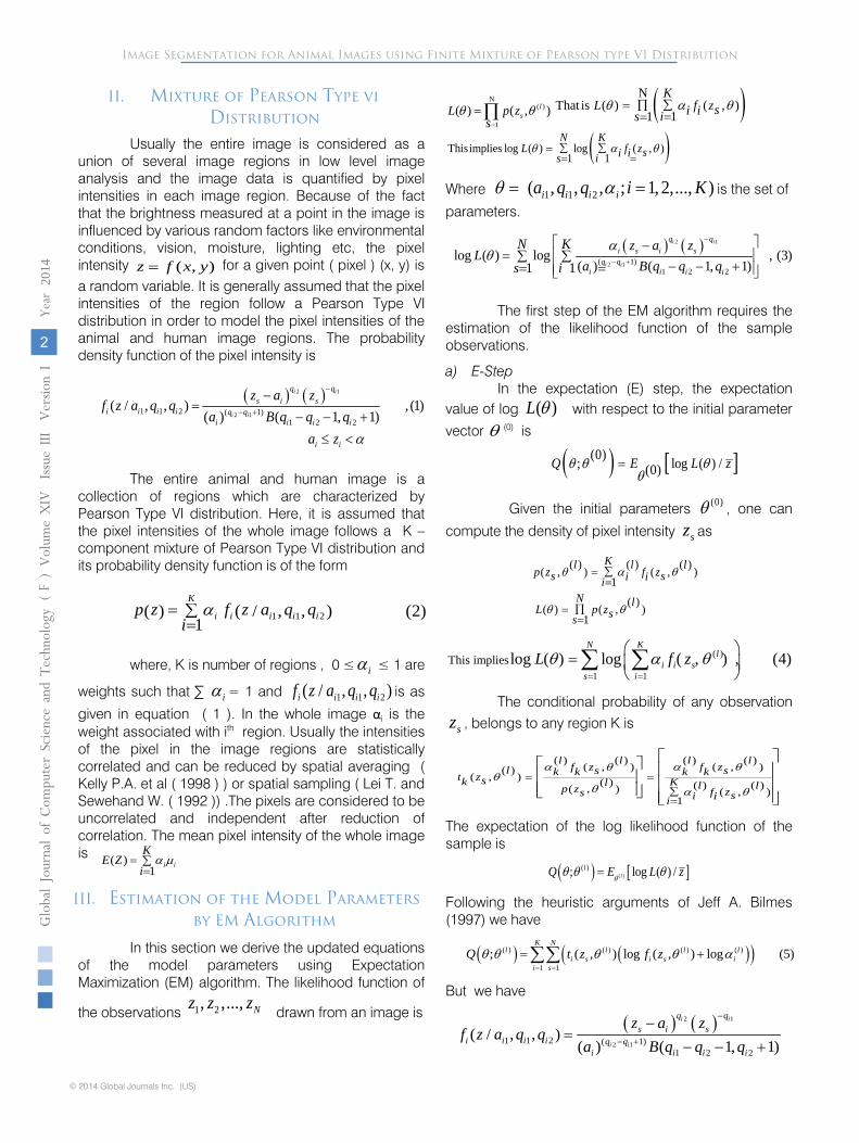
Usually the entire image is considered as a

union of several image regions

in low level image analysis and the image data is quantified by pixel intensities in each image region. Because of the fact that the brightness measured at a point in the image is influenced by various random factors like environmental conditions, vision,

moisture, lighting etc, the pixel

intensity ( , )z f x y= for a given point ( pixel ) (x, y) is

a random variable. It is generally assumed that the pixel intensities of the region follow a Pearson Type VI distribution in order to model the pixel intensities of the animal and human image regions.

The probability

density function of the pixel intensity is

( ) ( )2 1

2 11 1 2 ( 1)1 2 2

( / , , )( ) ( 1, 1)

i i

i i

q qs i s

i i i i q qi i i i

i i

z a zf z a q q

a B q q qa z α

−

− +

−=

− − +≤ <

The entire animal and human image is a

collection of regions which are characterized by Pearson Type VI distribution. Here, it is assumed that the pixel intensities of the whole image follows a K – component mixture of Pearson Type VI distribution and its probability density function is of the form

1 1 2( ) ( / , , ) (2)1

K

i i i i ip z f z a q qi

α= ∑=

where, K is number of regions , 0 ≤ iα ≤ 1 are

weights such that ∑ iα = 1 and 1 1 2( / , , )i i i if z a q q is as

given in equation ( 1 ). In the whole image αi is the weight associated with ith region. Usually the intensities of the pixel in the image regions are statistically correlated and can be reduced by spatial averaging ( Kelly P.A. et al ( 1998 ) ) or spatial sampling ( Lei T. and Sewehand W. ( 1992 )) .The pixels are considered to be uncorrelated and independent after reduction of correlation. The mean pixel intensity of the whole image is ( )

1 i i

KE Z

iα µ= ∑

=

III. Estimation of the Model Parameters by EM Algorithm

In this section we derive the updated equations of the model parameters using Expectation Maximization (EM) algorithm. The likelihood function of

the observations 1 2, ,..., Nz z z drawn from an image is

N( )

1

( ) ( , )lsL p z

sθ θ

=

=∏ ( )NThat is ( ) ( , )

11∑∏===

KL f zsi iisθ α θ

( )Thisimplies log ( ) log ( , )1 1

∑ ∑== =

N KL f zsi is iθ α θ

Where 1 1 2 ( , , , ; 1, 2,..., )i i i ia q q i Kθ α= = is the set of

parameters.

( ) ( )2 1

2 1( 1)1 2 2

log ( ) log , (3)( ) ( 1, 1)1 1

i i

i i

q qi s i s

q qi i i i

N K z a zL

a B q q qs iα

θ−

− +

−= ∑ ∑

− − += =

The first step of the EM algorithm requires the estimation of the likelihood function of the sample observations.

a) E-Step In the expectation (E) step, the expectation

value of log ( )L θ with respect to the initial parameter

vector θ (0) is

( ) [ ](0); log ( ) /(0)=Q E L zθ θ θθ

Given the initial parameters (0)θ , one can

compute the density of pixel intensity sz as

( ) ( ) ( )( , ) ( , ) 1

( ) ( ) ( , )1

Kl l lp z f zs si iiN lL p zss

θ α θ

θ θ

∑==

∏==

( )

1 1This implieslog ( ) log ( , ) , (4)

= =

=

∑ ∑N K

li i s

s iL f zθ α θ

The conditional probability of any observation

sz , belongs to any region K is

( ) ( ) ( ) ( )( , ) ( , )( )( , ) ( ) ( ) ( )( , ) ( , )1

= =∑=

l l l lf z f zl s sk k k kt zsk Kl l lp z f zs si ii

α θ α θθ

θ α θ

The expectation of the log likelihood function of the sample is

( ) [ ]( )( ); log ( ) /llQ E L z

θθ θ θ=

Following the heuristic arguments of Jeff A. Bilmes (1997) we have

( ) ( )( )( ) ( ) ( ) ( )

1 1; ( , ) log ( , ) log (5)

= =

= +∑∑K N

l l l li s i s i

i sQ t z f zθ θ θ θ α

But we have

( ) ( )2 1

2 11 1 2 ( 1)1 2 2

( / , , )( ) ( 1, 1)

i i

i i

q qs i s

i i i i q qi i i i

z a zf z a q q

a B q q q

−

− +

−=

− − +



, (1)

Globa

l Jo

urna

l of C

ompu

ter Sc

ienc

e an

d Te

chno

logy

V

olum

e XIV

Issu

e III

Versio

n I

2

(

DDDD)

Year

2014

F

II. Mixture of Pearson Type viDistribution

( ) ( )( )( ) ( ) ( ) ( ); ( , ) log ( , ) log1 1

K Nl l l lQ t z f zs si i ii sθ θ θ θ α∑ ∑= +

= =

b) M-Step

For obtaining the estimation of the model parameters one has to maximize ( )( ); lQ θ θ such that

∑αi= 1. This can be solved by applying the standard solution method for constrained maximum by constructing the first order Lagrange type

function,

( )( ) ( )(log ( )) 1 (6)1

Kl lS E L iiθ λ α∑= + −

=

where, λ is Lagrangian multiplier combining the constraint with the log likelihood function to be maximized.

Hence,

0∂

=∂

Siα

. This implies

( ) ( )2 1

2 1

( )i ( 1)

1 1 1 2 2

1

( , ) log log ( ) ( 1, 1)

1 0

i i

i i

q qK Ns i sl

i s q qi si i i i i

K

ii

z a zt z

a B q q qθ α

α

λ α

−

− += =

=

−∂ + ∂ − − +

+ − =

∑∑

∑

This implies1

1 ( )( , ) 0i si

N lt zi

θ λα

+ =∑=

Summing both sides over all observations, we

get λ = -N Therefore ( )

1

1 ( , )∧

=

= ∑N

li i s

st z

Nα θ The updated

equation of iα for ( l +1)th iteration is

( )1 ( )

1

1 ( , )N

l li i s

st z

Nα θ+

=

= ∑

( )1( ) ( )

( , )1

( ) ( )1 ( , )1

li

l lN f zi i sK l lsN f zi i si

α θ

α θα +

∑= ∑

=

=

(7)

Therefore ( )( ); 0l

i

Qa

θ θ∂=

∂ implies ( )

1

log ( ; ) 0l

i

LEaθ θ ∂

= ∂

( )( )( ) ( ) ( )

1 1( , ) log ( , ) log 0

K Nl l l

i s i s ii si

t z f za

θ θ α= =

∂ + =∂ ∑∑

The updated equation of ia at ( l +1)th iteration is

( )2 1

2

( ) ( ) ( ) ( )( 1)

( ) ( )1

( 1) ( , )

( , )i i i

i

i

l l l lNs i sll l

s i s

q q z a t za

t z q

θ

θ+

=

− − + − =

∑

For updating the parameter 1iq , i = 1, 2, …, K

we consider the derivative of ( )( ); lQ θ θ with respect to

1iq and equate it to zero. We have

( )( ) ( ); log ( ; )l lQ E Lθ θ θ θ =

Therefore ( )( )

1

; 0l

i

Qq

θ θ∂=

∂

implies ( )

1

log ( ; ) 0l

i

LEqθ θ ∂

= ∂

( )( )( ) ( ) ( )

1 11

( , ) log ( , ) log 0K N

l l li s i s i

i si

t z f zq

θ θ α= =

∂ + = ∂ ∑∑

( )

11 ( )

0 1 2 0 1

( , )1 (8)log ( 2 1) ( 1) ( , )

lNi s

is li

i i i i ss

t zqa q q q t zz

θ

ψ ψ θ=

= − − − − + + −

∑

The updated equation of 1iq at ( l +1)th

iteration is

1

1 2 1

( )( 1)

1 ( ) ( ) ( ) ( )0 0

( , )1 (9)log ( 2 1) ( 1) ( , )

i

i i i

lNl i s

s l l l lii s

s

t zqa q q q t zz

θ

ψ ψ θ

+

=

= − − − − + + −

∑

For updating the parameter 2iq , i = 1, 2, …,

K we consider the derivative of ( )( ); lQ θ θ with respect

to 2iq and equate it to zero. We have

( )( ) ( ); log ( ; )l lQ E Lθ θ θ θ =

Therefore ( )( )

2

; 0l

i

Qq

θ θ∂=

∂implies ( )

2

log ( ; ) 0l

i

LEqθ θ ∂

= ∂

( )( )( ) ( ) ( )

1 12

( , ) log ( , ) log 0K N

l l li s i s i

i si

t z f zq

θ θ α= =

∂ + = ∂ ∑∑

( )

12

( )0 1 2 0 2

1

( , )(10)

( )log ( 2 1) ( ) ( , )

Nl

i ss

i Nls i

i i i i ss i

t zq

z a q q q t za

θ

ψ ψ θ

=

=

= −

+ − − + −

∑

∑

The updated equation of 2iq at ( l +1)th iteration is

2

1 2 2

( )

( 1) 1

( ) ( ) ( ) ( )0 0

1

( , )(11)

( )log ( 2 1) ( ) ( , )i

i i i

Nl

i sl s

Nl l l ls i

i ss i

t zq

z a q q q t za

θ

ψ ψ θ

+ =

=

= −

+ − − + −

∑

∑

Where ( ) ( )

( )

( ) ( )

1

( , )( , )( , )

l ll i i s

i s Kl l

i i si

f zt zf z

α θθα θ

=

=

∑

IV. Initialization of the Parameters by k

– Means and Hierarchical Algorithm

Generally the efficiency of the EM algorithm depends upon the count of the regions in the image, during the estimation of the parameters. The number of



Globa

l Jo

urna

l of C

ompu

ter Sc

ienc

e an

d Te

chno

logy

V

olum

e XIV

Issu

e III

Versio

n I

3

(DDDD DDDD

)Year

2014

F

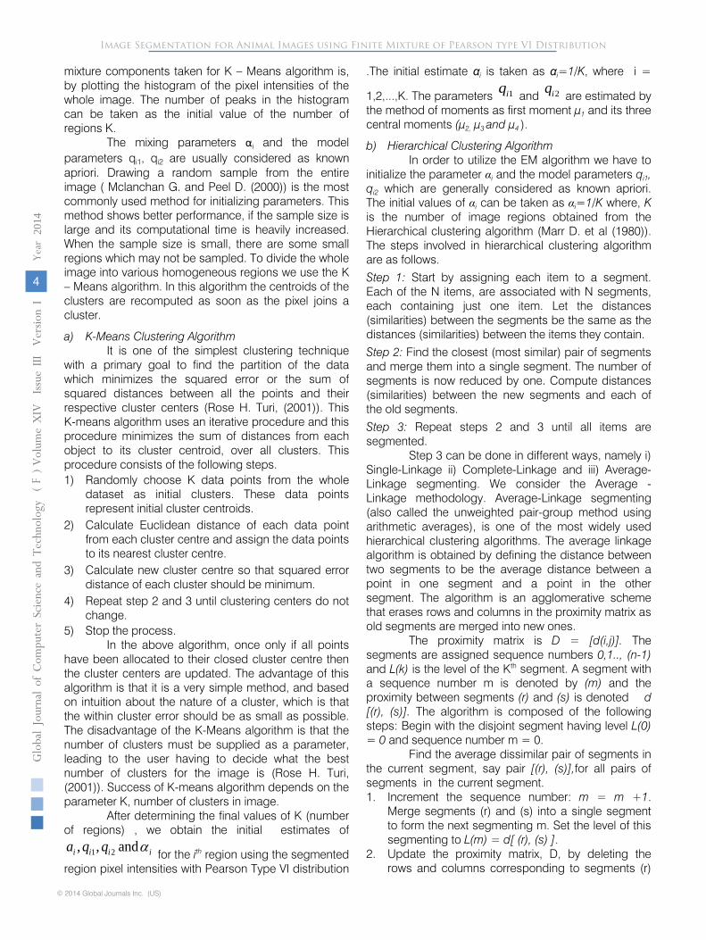
mixture components taken for K – Means algorithm is, by plotting the histogram of the pixel intensities of the whole image. The number of peaks in the histogram can be taken as the initial value of the number of regions K.

The mixing parameters αi and the model parameters qi1, qi2 are usually considered as known apriori. Drawing a random sample from the entire image ( Mclanchan G. and Peel D. (2000)) is the most commonly used method for initializing parameters. This method shows better performance, if the sample size is large and its computational time is heavily increased. When the sample size is small, there are some small regions which may not be sampled. To divide the whole image into various homogeneous regions we use the K – Means algorithm. In this algorithm the centroids of the clusters are recomputed as soon as the pixel joins a cluster.

a) K-Means Clustering Algorithm It is one of the simplest clustering technique

with a primary goal to find the partition of the data which minimizes the squared error or the sum of squared distances between all the points and their respective cluster centers (Rose H. Turi, (2001)). This K-means algorithm uses an iterative procedure and this procedure minimizes the sum of distances from each object to its cluster centroid, over all clusters. This procedure consists of the following steps. 1) Randomly choose K data points from the whole

dataset as initial clusters. These data points represent initial cluster centroids.

2) Calculate Euclidean distance of each data point from each cluster centre and assign the data points to its nearest cluster centre.

3) Calculate new cluster centre so that squared error distance of each cluster should be minimum.

4)

Repeat step 2 and 3 until clustering centers do not change.

5)

Stop the process.

In the above algorithm, once only if all points have been allocated to their closed cluster centre then the cluster centers are updated. The advantage of this algorithm is that it is a very simple method, and based on intuition about the nature of a cluster, which is that the within cluster error should be as small as possible. The disadvantage of the K-Means algorithm is that the number of clusters must be supplied as a parameter, leading to the user having to decide what the best number of clusters for the image is (Rose H. Turi, (2001)). Success of K-means algorithm depends on the parameter K, number of clusters in image.

After determining the final values of K (number of regions) , we obtain the initial estimates of

1 2, , andi i i ia q q α for the ith

region using the segmented

region pixel intensities with Pearson Type VI distribution

.The initial estimate αi is taken as αi=1/K, where i =

1,2,...,K. The parameters 1iq and 2iq

are estimated by the method of moments as first moment µ1 and its three central moments (µ2, µ3 and µ4 ).

b) Hierarchical Clustering Algorithm In order to utilize the EM algorithm we have to

initialize the parameter αi and the model parameters qi1, qi2 which are generally considered as known apriori. The initial values of αi can be taken as αi=1/K where, K is the number of image regions obtained from the Hierarchical clustering algorithm (Marr D. et al (1980)). The steps involved in hierarchical clustering algorithm are as follows. Step 1: Start by assigning each item to a segment. Each of the N items, are associated with N segments, each containing just one item. Let the distances (similarities) between the segments be the same as the distances (similarities) between the items they contain. Step 2: Find the closest (most similar) pair of segments and merge them into a single segment. The number of segments is now reduced by one. Compute distances (similarities) between the new segments and each of the old segments. Step 3: Repeat steps 2 and 3 until all items are segmented.

Step 3 can be done in different ways, namely i) Single-Linkage ii) Complete-Linkage and iii) Average-Linkage segmenting. We consider the Average -Linkage methodology. Average-Linkage segmenting (also called the unweighted pair-group method using arithmetic averages), is one of the most widely used hierarchical clustering algorithms. The average linkage algorithm is obtained by defining the distance between two segments to be the average distance between a point in one segment and a point in the other segment. The algorithm is an agglomerative scheme that erases rows and columns in the proximity matrix as old segments are merged into new ones.

The proximity matrix is D = [d(i,j)]. The segments are assigned sequence numbers 0,1.., (n-1) and L(k) is the level of the Kth segment. A segment with a sequence number m is denoted by (m) and the proximity between segments (r) and (s) is denoted d [(r), (s)]. The algorithm is composed of the following steps: Begin with the disjoint segment having level L(0) = 0 and sequence number m = 0.

Find the average dissimilar pair of segments in the current segment, say pair [(r), (s)],for all pairs of segments in the current segment. 1. Increment the sequence number: m = m +1.

Merge segments (r) and (s) into a single segment to form the next segmenting m. Set the level of this segmenting to L(m) = d[ (r), (s) ].

2. Update the proximity matrix, D, by deleting the rows and columns corresponding to segments (r)



Globa

l Jo

urna

l of C

ompu

ter Sc

ienc

e an

d Te

chno

logy

V

olum

e XIV

Issu

e III

Versio

n I

4

(DDDD

)Year

2014

F

and (s) and adding a row and column corresponding to the newly formed segment. The proximity between the new segment, denoted (r, s) and old segment( K )is defined in this way.

i j

(r,s) K

(r,s) K

d(i,j)

N Nd =

∑∑

where d(i, j) is the distance between object i in the cluster ( r, s ) and object j in the cluster K, and N(r,s) and N(k) are the number of items in the clusters ( r, s ) and K respectively. The above procedure is repeated till the distance between two clusters is less than the specified threshold value.

We obtain the initial estimates of qi1, qi2 and αi for the ith region using the segmented region pixel intensities with the moment method given by Pearsonian Type VI distribution, only after determining the final values of K (number of regions). After getting these initial estimates, the final refined estimates of the parameters through EM algorithm given in section (III) is obtained.

V. Segmentation Algorithm

In this section, the characteristics of the image segmentation algorithm are projected. After refining the parameters, the first step in image segmentation is allocating the pixels to the segments of the image. This operation is performed by Segmentation Algorithm which consists of four steps. Step 1: Plot the histogram of the whole image. Step 2: Obtain the initial estimates of the model parameters using K-Means algorithm and moment estimates for each image region as discussed in section IV. Step 3: Obtain the refined estimates of the model parameters qi1,qi2 and αi for i=1, 2, ..., K using the EM algorithm with the updated equations given by (7), (9) and (11) respectively in section III. Step 4: Assign each pixel into the corresponding jth region (segment) according to the maximum likelihood of the jth component Lj. That is

,

( ) ( )2 1

2 1j ( 1) 1 2 2

L ( ) ( 1, 1) max

j j

j j

q qs i s

q qj k j j j j

z a za q q qβ

−

− +∈

−=

− − +

1 2, .i i j ja z q qα≤ < −∞ < < ∞

VI. Experimental Results

The performance of the developed a segmentation method for the natural images, which are considered on the earth. For implementing this algorithm, we need to initialize the model parameters, which are usually done by using moment method of estimations. Initially the feature vector is divided into

different segmented regions by making use of non-parametric methods of segmentation namely K-means algorithm and Hierarchical clustering algorithms.

An experiment is conducted with four images taken from Berkeley images dataset (http:// www. eecs. berkeley.edu/Research/Projects/CS/Vision/bsds/BSDS300/html). The images FACE, EAGLE, NEST BIRD and TIGER, are considered for image segmentation in order to demonstrate the utility of the image segmentation algorithm. The pixel intensities of the whole image are taken as feature. The pixel intensities of the image are always assumed to follow a mixture of Pearson Type VI distribution.

That is, the image contains K regions and pixel intensities in each image region follow a Pearson Type VI distribution with different parameters. The number of segments in each of the four images considered for experimentation are determined by the histogram of pixel intensities. The histograms of the pixel intensities of the four images are shown in Figure 1.

TIGER

EAGLE

NEST BIRD

FACE

Figure 1 : Histograms Of The Images

The initial estimates of the number of the regions K in each image are obtained and given in Table 1.

Table 1 : Initial Estimates Of K

IMAGE

TIGER

EAGLE NEST

BIRD FACE

Estimate of K 2

3

4

4

From Table 1, we observe that the image TIGER has two segments, images EAGLE has three segments and images NEST BIRD AND FACE have four segments each. The initial values of the model parameters mi1,mi2, qi1,qi2 and αi for i = 1, 2, …, K , for each image region are computed by the method given in section III.

By making use of these initial estimates and the updated equations of the EM Algorithm given in Section III, the final estimates of the model parameters for each image

are obtained and presented in Tables 2.a,2.b, 2.c, and 2.d for different images.



Globa

l Jo

urna

l of C

ompu

ter Sc

ienc

e an

d Te

chno

logy

V

olum

e XIV

Issu

e III

Versio

n I

5

(DDDD DDDD

)Year

2014

F

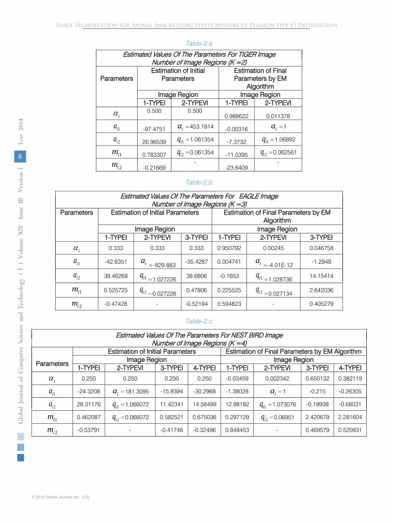
Estimated Values Of The Parameters For EAGLE Image

Number of Image Regions (K =3)

Parameters

Estimation of Initial Parameters

Estimation of Final Parameters by EM Algorithm

Image Region

Image Region

1-TYPEI

2-TYPEVI

3-TYPEI

1-TYPEI

2-TYPEVI

3-TYPEI

iα

0.333

0.333

0.333

0.950792

0.00245

0.046758

1ia

-42.6351

ia=-829.883

-35.4287

0.004741

ia=-4.01E-12

-1.2948

2ia

38.46268

1iq=1.027226

38.6806

-0.1653

1iq=1.028736

14.15414

1im

0.525725

2iq=0.027226

0.47806

0.225525

2iq=0.027134

2.642036

2im

-0.47428

-

-0.52194

0.594823

-

0.405279

Estimated Values Of The Parameters For TIGER Image


Parameters

Estimation of Initial

Parameters

Estimation of Final Parameters by EM

Algorithm

Image Region

Image Region

1-TYPEI

2-TYPEVI

1-TYPEI

2-TYPEVI

iα

0.500

0.500

0.988622

0.011378

1ia

-97.4751

ia =453.1814

-0.00316

ia =1

2ia

26.96539

1iq =1.061354

-7.3732

1iq =1.06892

1im

0.783307

2iq =0.061354

-11.0395

2iq =0.062561

2im

-0.21669

-

-23.8409

-

Estimated Values Of The Parameters For NEST BIRD Image


Parameters

Estimation of Initial Parameters


Image Region

Image Region

1-TYPEI

2-TYPEVI

3-TYPEI

4-TYPEI

1-TYPEI

2-TYPEVI

3-TYPEI

4-TYPEI

iα

0.250

0.250

0.250

0.250

-0.03459

0.002342

0.650132

0.382119

1ia

-24.3208

ia =181.3095

-15.9394

-30.2968

-1.38028

ia =1

-0.215

-0.26305

2ia

28.31176

1iq =1.066072

11.42341

14.58499

12.98182

1iq =1.073076

-0.19938

-0.68031

1im

0.462087

2iq =0.066072

0.582521

0.675036

0.297129

2iq =0.06951

2.420679

2.281604

2im

-0.53791

-

-0.41748

-0.32496

0.848453

-

0.469579

0.520931



Globa

l Jo

urna

l of C

ompu

ter Sc

ienc

e an

d Te

chno

logy

V

olum

e XIV

Issu

e III

Versio

n I

6

(

DDDD)

Year

2014

F

Table-2.a

Table-2.b

Table-2.c

The probability density function of pixel

intensities of each image is estimated by substituting the final estimates of the model parameters. The estimated probability density function of the pixel intensities of the image TIGER is

( ) ( )

11.04 23.8411.04 23.84

11.0395 23.8409

0.06256

( ) ( )

( )(

1 1.

1)

06892

0.988622 0.00316 7.370.0032 7.

( )( ) ( ) 1 1( , )

( ) ( 1, 1)

( ) 1.

3730.

000(1.

00316 7.3732 11.0395 23.841

0.011378

i i

ls

s s

z z

f z

z z

θβ+ +

−

− −− −

− −

− −− −

−

+ − = +

+

−

− +− −

0.0626 1.06892( 1) 1.06892 0.06256000) ( 1 0.06 6, 2 1)β− + − − +

The estimated probability density function of the pixelintensities of the image EAGLE is

( )

( )

( ) ( )( ) (

0.226 0.5950.226 0.5948)

0.2255 0.( )

5948

0.06

1)

1

(

256

0.950792 0.005 0.16530.005 0.1653

0.0047 0.1653 0.225525 0

( )( ) ( ) 1 1,

( ) ( 1, 1)

( )

.5948

0.00245 4.01 1

2

i i

ls

s

z z

f z

zEz

θβ+ +

+ − =

+ + +

−+

−−

−

− ( )( 1)

( ) ( )( )

1.028736

0.027134 1.028736

2.6421 0.412.64204 0.41

2.642036 0.40527

)

( 1)9

(

4.01 12 1.028736 0.027134 0.02713

0.046758 1.2948 14.

( ) ( 1, 1)

( )( ) 1541.2948 14.154

1.2948 14.154

( ) 1 1

( ) 2(

s

i iz z

E β

β

− +

+ +

− − +

+ −

−

+

+ 1,.642036 0.405 13 )+ +

The estimated probability density function of the pixel intensities of the image NEST BIRD is

( )

( )

(0.2971) (0.849)(0.29713) (0.8485)

( )(0.29713 0.8485 1)

0.06951

(-0.03459)(-1.38) (12.982) 1 1-1.381 12.982

, (-1.38028 12.98182) (0.2972 1,0.849 1)

(0.002342) 1.000

i i

ls

s

z z

f z

z z

θβ+ +

+ −

=+ + +

−+

( )1.073076

(0.06951 1.073076 1)

(2.4207) (0.469)(2.421) (0.4696)

(2.420679 0.4696 1)

(1.000) (0.06951 1,0.06951 1)

(0.650132)(-0.215) (-0.1994) 1 1-0.215 -0.1994

(-0.215-0.19938

0.

) (2.42

062561s

i iz z

β

β

− +

+ +

− − +

+ − +

(2.282) (0.521)(2.282) (0.521)

(2.281604 0.520931 1)

0679 1,0.4696 1)

(0.382119)(-0.2631) (-0.680) 1 1-0.263 -0.68031

(-0.26305-0.68031) (2.281604 1,0.5209 1)

i iz z

β+ +

+ +

+ − +

+ +

The estimated probability density function of the pixel intensities of the image FACE is

( )

(-0.028) (-0.082)(-0.0283) (-0.0819)

( )(-0.0283-0.0819 1)

(2.4305)

(0.0068)(20.61) (493.75) 1 120.607 493.75,

(20.6072 493.753) (-0.0283 1, -0.082 1)

(0.9772)(-0.1116) (

i i

ls

z z

f z θβ+

+ − =

+ + +

+

( ) ( )

(2.431) (0.47)(0.47)

(2.4305 0.4662 1)

0.0475 1.055

(0.0475 1.055 1)

-0.3840) 1 1-0.1116 -0.384

(-0.1116-0.3840) (2.4305 1,0.4662 1)

(0.0078) 1.000 (1.000) (1.055 0.0475 1,0.0475 1)

(0.008

i i

s s

z z

z z

β

β

+ +

− +

+ −

+ +

−+

− − +

+

(2.664) (0.3995)(2.664) (0.3995)

(2.664 0.3995 1)

2)(-2.29) (15.58) 1 1-2.290 15.58

(-2.290 15.58) (2.664 1,0.3995 1)

i iz z

β+ +

+ −

+ + +

Using the estimated probability density function and image segmentation algorithm given in section III, the image segmentation is done for the five images under consideration. The original and

segmented images are shown in Figure 2

Figure 2 :

Original and Segmented Images

ORIGINAL IMAGES

SEGMENTED

IMAGES

Estimated Values Of The Parameters For FACE Image


Parameters Estimation of Initial Parameters Estimation of Final Parameters by EM

Algorithm Image Region Image Region

1-TYPEI 2-TYPEI 3-TYPEVI 4-TYPEI 1-TYPEI 2-TYPEI 3-TYPEVI 4-TYPEI

iα 0.250 0.250 0.250 0.250 0.0068 0.9772 0.0078 0.0082

1ia

-18.965 -24.176 ia = -468.346 -16.528 20.6072 -0.1116 ia =1.000 -2.290

2ia

22.946 17.734 1iq = 1.047 18.557 493.753 -0.3840 1iq =-1.055 15.577

1im 0.4525 0.5768 2iq = 0.0471 0.4710 -0.0283 2.4305 2iq =0.0475 2.664

2im

-0.5474

-0.423

-

-0.5289

-0.0819

0.4662

-

0.3995



Globa

l Jo

urna

l of C

ompu

ter Sc

ienc

e an

d Te

chno

logy

V

olum

e XIV

Issu

e III

Versio

n I

7

(DDDD DDDD

)Year

2014

F

Table-2.d

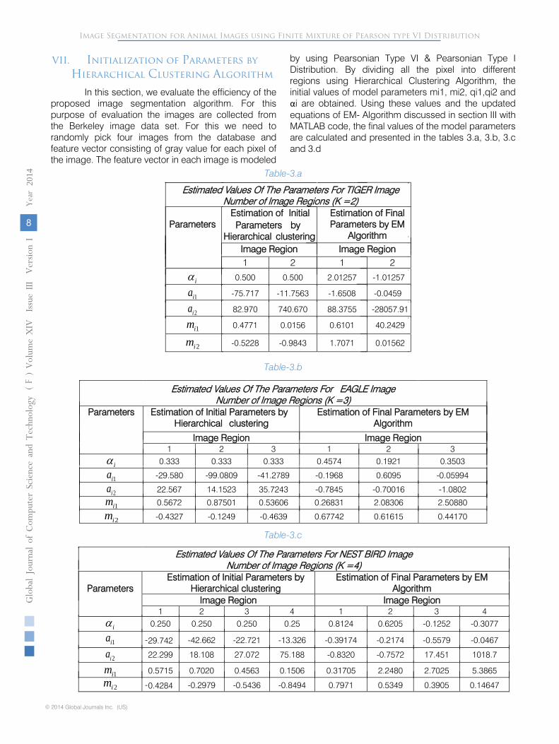
VII. Initialization of Parameters by

Hierarchical Clustering Algorithm

In this section, we evaluate the efficiency of the proposed image segmentation algorithm. For this purpose of evaluation the images are collected from the Berkeley image data set. For this we need to randomly pick four images from the database and feature vector consisting of gray value for each pixel of the image. The feature vector in each image is modeled

by using Pearsonian Type VI & Pearsonian Type I Distribution. By dividing all the pixel into different regions using Hierarchical Clustering Algorithm, the initial values of model parameters mi1, mi2, qi1,qi2 and αi are obtained. Using these values and the updated equations of EM- Algorithm discussed in section III with MATLAB code, the final values of the model parameters are calculated and presented in the tables 3.a, 3.b, 3.c and 3.d

Estimated Values Of The Parameters For TIGER Image Number of Image Regions (K =2)

Parameters

Estimation of Initial Parameters by

Hierarchical clustering

Estimation of Final Parameters by EM

Algorithm Image Region

Image Region

1

2

1

2

iα

0.500

0.500

2.01257

-1.01257

1ia

-75.717

-11.7563

-1.6508

-0.0459

2ia

82.970

740.670

88.3755

-28057.91

1im

0.4771

0.0156

0.6101

40.2429

2im

-0.5228

-0.9843

1.7071

0.01562

Estimated Values Of The Parameters For EAGLE Image


Parameters

Estimation of Initial Parameters byHierarchical clustering


Image Region

Image Region

1

2

3

1

2

3

iα

0.333

0.333

0.333

0.4574

0.1921

0.3503

1ia

-29.580

-99.0809

-41.2789

-0.1968

0.6095

-0.05994

2ia

22.567

14.1523

35.7243

-0.7845

-0.70016

-1.0802

1im

0.5672

0.87501

0.53606

0.26831

2.08306

2.50880

2im

-0.4327

-0.1249

-0.4639

0.67742

0.61615

0.44170


Estimated Values Of The Parameters For NEST BIRD ImageNumber of Image Regions (K =4)

ParametersEstimation of Initial Parameters by

Hierarchical clusteringEstimation of Final Parameters by EM

AlgorithmImage Region Image Region

1 2 3 4 1 2 3 4

iα 0.250 0.250 0.250 0.25 0.8124 0.6205 -0.1252 -0.3077

1ia -29.742 -42.662 -22.721 -13.326 -0.39174 -0.2174 -0.5579 -0.0467

2ia 22.299 18.108 27.072 75.188 -0.8320 -0.7572 17.451 1018.7

1im 0.5715 0.7020 0.4563 0.1506 0.31705 2.2480 2.7025 5.3865

2im -0.4284 -0.2979 -0.5436 -0.8494 0.7971 0.5349 0.3905 0.14647


Globa

l Jo

urna

l of C

ompu

ter Sc

ienc

e an

d Te

chno

logy

V

olum

e XIV

Issu

e III

Versio

n I

8

(

DDDD)

Year

2014

F

Table-3.a

Table-3.b

Table-3.c

Substituting the final estimates of the model parameters, the probability density function of pixel intensities of each image is estimated.

The estimated probability density function of the pixel intensities of the image TIGER is

( )

(0.6101) (1.7071)(0.6101) (1.7071)

( )(0.6101 1.7071 1)

(2.01257)(-1.6508) (88.3755) 1 1-1.6508 88.3755,

(-1.6508 88.3755) (0.6101 1,1.7071 1)

(-1.01257)(-0.0459

i i

ls

z z

f z θβ+ +

+ − =

+ + +

+

(40.2429) (0.01562)(40.2429) (0.01562)

(40.2429 0.01562 1)

) (-28057.91) 1 1-0.0459 -28057.91

(--0.0459 -28057.91) (40.2429 1,0.01562 1)

i iz z

β+ +

+ −

+ + +

The estimated probability density function of the pixel intensities of the image EAGLE is

The estimated probability density function of the pixel intensities of the image NEST BIRD is

( )

(0.31705) (0.7971)(0.31705) (0.7971)

( )(0.31705 0.7971 1)

(

(0.8124)(-0.39174) (-0.8320) 1 1-0.39174 -0.8320,

(-0.39174 -0.8320) (0.31705 1,0.7971 1)

(0.6205)(-0.2174)

i i

ls

z z

f z θβ+ +

+ − =

+ + +

+

(2.2480) (0.5349)2.2480) (0.5349)

(2.2480 0.5349 1)

(2.7025)(2.7025) (0.39047)

(-0.7572) 1 1-0.2174 -0.7572

(-0.2174 -0.7572) (2.2480 1,0.5349 1)

(-0.1252)(-0.5579) (17.4509) 1 1-0.5579

i i

i

z z

z

β+ +

+ −

+ + +

+ +

(0.39047)

(2.7025 0.39047 1)

(5.3865) (0.14647)(5.3865) (0.14647)

(5.38

17.4509(-0.5579 17.4509) (2.7025 1,0.39047 1)

(-0.30771)(-0.04669) (1018.7) 1 1-0.04669 1018.7

(-0.04669 1018.7)

i

i i

z

z z

β+ +

−

+ + +

+ − +

+ 65 0.14647 1) (5.3865 1,0.14647 1)β+ + + +

( )

(0.2683) (0.6774)(0.2683) (0.6774)

( )(0.26831 0.6774 1)

(2.0831

(0.4574)(-0.1968) (-0.7845) 1 1-0.1968 -0.7845,

(-0.1968 -0.7845) (0.26831 1,0.6774 1)

(0.1921)(0.6095)

i i

ls

z z

f z θβ+ +

+ − =

+ + +

+

(2.0831) (0.6162)) (0.6162)

(2.08306 0.61615 1)

(2.5088)(2.5088) (0.442)

(-0.70016) 1 10.6095 -0.70016

(0.6095 -0.70016) (2.08306 1,0.6162 1)

(0.3503)(-0.05994) (-1.0802) 1 1-0.05994

i i

i i

z z

z z

β+ +

+ −

+ + +

+ − +

(0.4417)

(2.5088 0.4417 1)-1.0802

(-0.05994 -1.0802) (2.5088 1,0.4417 1)β+ +

+ + +

Estimated Values Of The Parameters For FACE Image


Parameters

Estimation of Initial Parameters by Hierarchical clustering


Image Region

Image Region

1 2 3 4 1 2 3 4

iα

0.250

0.250

0.250

0.250

0.3736

0.2847

0.2526

0.0891

1ia

-12.244

-12.556

-14.509

-68.801

-0.0611

-0.1155

-0.0811

1.5517

2ia

71.505

11.0781

9.1209

57.659

2536.35

0.3296

0.1468

-5.4401

1im

0.1462

0.5312

0.6140

0.544

-0.3232

2.5188

2.3684

2.4925

2im

- 0.8537

-0.4687

-0.3859

-0.4559

-2.3224

0.4387

0.4876

0.4465


( )

(4.1042) (13.844)(4.1042) (13.844)

( )(4.1042 13.844 1)

(2.987

(-0.6508)(-0.2402) (1504.84) 1 1-0.2402 1504.84,

(-0.2402 1504.84) (4.1042 1,13.844 1)

(-0.2327)(-0.1752)

i i

ls

z z

f z θβ+ +

+ − =

+ + +

+

(2.9874) (0.3331)4) (0.3331)

(2.9874 0.3331 1)

(2.3041)(2.3041) (0.51185)

(-622.13) 1 1-0.1752 -622.13

(-0.1752 -622.13) (2.9874 1,0.3331 1)

(0.7248)(-96.5481) (-5.9734) 1 1-96.5481 -

i i

i i

z z

z z

β+ +

+ −

+ + +

+ − +

(0.51185)

(2.3041 0.51185 1)

(2.34037) (0.4979)(2.34037) (0.4979)

(2.34037 0

5.9734(-96.5481 -5.9734) (2.3041 1,0.51185 1)

(1.1587)(-0.3530) (-0.7436) 1 1-0.3530 -0.7436

(-0.3530 -0.7436)

i iz z

β+ +

+

+ + +

+ − +

+ .4979 1) (2.34037 1,0.4979 1)β+ + +

( )

(4.1042) (13.844)(4.1042) (13.844)

( )(4.1042 13.844 1)

(2.987

(-0.6508)(-0.2402) (1504.84) 1 1-0.2402 1504.84,

(-0.2402 1504.84) (4.1042 1,13.844 1)

(-0.2327)(-0.1752)

i i

ls

z z

f z θβ+ +

+ − =

+ + +

+

(2.9874) (0.3331)4) (0.3331)

(2.9874 0.3331 1)

(2.3041)(2.3041) (0.51185)

(-622.13) 1 1-0.1752 -622.13

(-0.1752 -622.13) (2.9874 1,0.3331 1)

(0.7248)(-96.5481) (-5.9734) 1 1-96.5481 -

i i

i i

z z

z z

β+ +

+ −

+ + +

+ − +

(0.51185)

(2.3041 0.51185 1)

(2.34037) (0.4979)(2.34037) (0.4979)

(2.34037 0

5.9734(-96.5481 -5.9734) (2.3041 1,0.51185 1)

(1.1587)(-0.3530) (-0.7436) 1 1-0.3530 -0.7436

(-0.3530 -0.7436)

i iz z

β+ +

+

+ + +

+ − +

+ .4979 1) (2.34037 1,0.4979 1)β+ + +

The estimated probability density function of the pixel intensities of the image FACE is

( )

(-0.3232) (1.0010)(-0.3232) (1.0010)

( )(-0.3232 1.0010 1)

(2.5

(0.3736)(-0.0611) (2536.35) 1 1-0.0611 2536.35,

(-0.0611 2536.35) (-0.3232 1,1.0010 1)

(0.2847)(-0.1155)

i i

ls

z z

f z θβ+ +

+ − =

+ + +

+

(2.5188) (0.4387)188) (0.4387)

(2.5188 0.4387 1)

(2.3684)(2.3684) (0.4876)

(0.3296) 1 1-0.1155 0.3296

(-0.1155 0.3296) (2.5188 1,0.4387 1)

(0.2526)(-0.0811) (0.1468) 1 1-0.0811 0.1468

i i

i i

z z

z z

β+ +

+ −

+ + +

+ − +

(0.4876)

(2.3684 0.4876 1)

(2.4925) (0.4465)(2.4925) (0.4465)

(2.4925 0.4465 1)

(-0.0811 0.1468) (2.3684 1,0.4876 1)

(0.0891)(1.5517) (-5.4401) 1 11.5517 -5.4401

(1.5517 -5.4401) (2.4925

i iz z

β

β

+ +

+ +

+ + +

+ − +

+ +1,0.4465 1)+

The estimated probability density function of the pixel intensities of the image BIRD is

Using the estimated probability density function and image segmentation algorithm given in section V, the image segmentation is done for the four images under consideration. The original and segmented images are shown in Figure 3.


Globa

l Jo

urna

l of C

ompu

ter Sc

ienc

e an

d Te

chno

logy

V

olum

e XIV

Issu

e III

Versio

n I

9

(DDDD DDDD

)Year

2014

F

Table-3.d

Figure 3 :

Original and Segmented Images

ORIGINAL IMAGES

SEGMENTED

IMAGES

VIII.

Performance

Evalution

In this paper we have conducted the experiment and also examined its performance by making use of the image segmentation algorithm. The performance evaluation of this segmentation technique is carried by obtaining the three performance measures

From Table 4 it is identified that the PRI values of the existing algorithm based on finite Gaussian Mixture model for the five images considered for experimentation are less than the values from the segmentation algorithm based Pearsonian Type VI Distribution with K-means. Similarly GCE and VOI values of the proposed algorithm are less than that of finite Gaussian mixture model. This reveals the fact that the proposed algorithm outperforms the existing algorithm based on the finite Gaussian mixture model.

After developing the image segmentation method , it is required to verify the utility of segmentation in model building of the image for image retrieval. By subjective image quality testing or by objective image quality testing the performance evaluation

of the retrieved image can be done. Since the numerical results of an objective measure allow a consistent comparison of different algorithms the objective image quality testing methods are often used. There are several image quality measures available for performance evaluation of the image segmentation method. An extensive survey of quality measures is given by Eskicioglu A.M. and Fisher P.S. (1995).

Using the estimated probability density functions of the images under consideration the


retrieved images are obtained and are shown in Figure 4.

namely, (i) probabilistic rand index (PRI), (ii) global consistence error (GCE) and (iii) variation of information (VOI). By computing the segmentation performance measures namely VOI, PRI and GCE for the five images under study using Pearsonian Type VI Distribution (PTVID-K), the performance of the developed algorithm is studied. The computed values of the performance measures for the developed algorithm and the earlier existing finite Gaussian mixture model(GMM) with K-means algorithm and Hierarchical algorithm are presented in Table 4 for a comparative study.

Table 4 : Segmentation Performace Measures

IMAGES METHODPERFORMACE

MEASURESPRI GCE VOI

TIGERGMM 0.8234 0.4956 2.568

PTVID-K 0.9896 0.4742 1.921PTVID-H 0.9897 0.4762 1.920

EAGLEGMM 0.8423 0.7006 8.354

PTVID-K 0.8505 0.7109 7.577PTVID-H 0.8627 0.7054 7.2002

Figure 4 : The Original and Retrieved Images

ORIGINAL IMAGES

RETRIEVED IMAGES

NEST BIRD

GMM 0.9793 0.9142 8.8837PTVID-K 0.0258 0.0124 6.7136PTVID-H 0.0074 0.0001 7.2132

FACEGMM 0.0201 0.0891 7.2546

PTVID-K 0.0223 0.0134 7.1556PTID-K 0.9559 0.8584 8.8772


Globa

l Jo

urna

l of C

ompu

ter Sc

ienc

e an

d Te

chno

logy

V

olum

e XIV

Issu

e III

Versio

n I

10

(

DDDD)

Year

2014

F

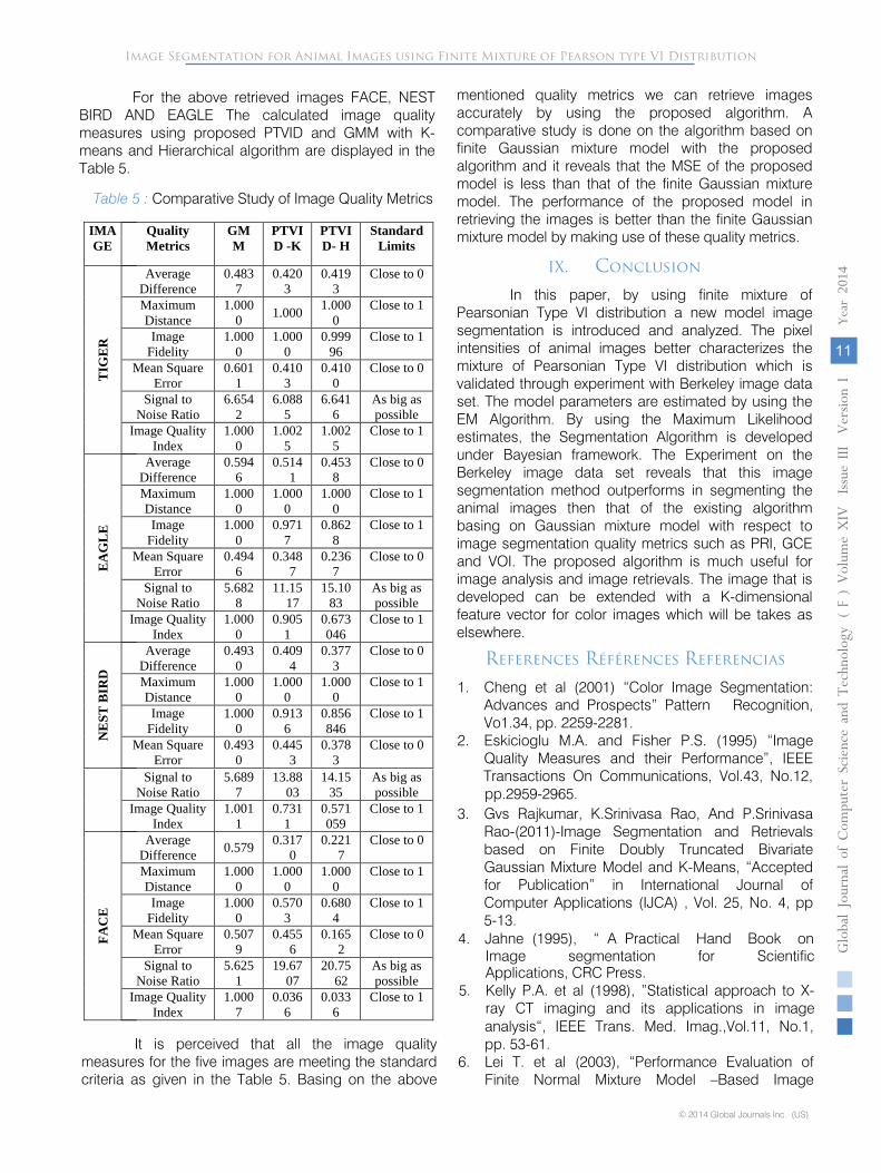
For the above retrieved images FACE, NEST BIRD AND EAGLE The calculated image quality measures using proposed PTVID and GMM with K-means and Hierarchical algorithm are displayed in the Table 5.

Table 5 :

Comparative Study of Image Quality Metrics


mentioned quality metrics we can retrieve images accurately by using the proposed algorithm. A comparative study is done on the algorithm based on finite Gaussian mixture model with the proposed algorithm and it reveals that the MSE of the proposed model is less than that of the finite Gaussian mixture model. The performance of the proposed model in retrieving the images is better than the finite Gaussian mixture model by making use of these quality metrics.

IX. Conclusion

In this paper, by using finite mixture of Pearsonian Type VI distribution a new model image segmentation is introduced and analyzed. The pixel intensities of animal images better characterizes the mixture of Pearsonian Type VI distribution which is validated through experiment with Berkeley image data set. The model parameters are estimated by using the EM Algorithm. By using the Maximum Likelihood estimates, the Segmentation Algorithm is developed under Bayesian framework. The Experiment on the Berkeley image data set reveals that this image segmentation method outperforms in segmenting the animal images then that of the existing algorithm basing on Gaussian mixture model with respect to image segmentation quality metrics such as PRI, GCE and VOI. The proposed algorithm is much useful for image analysis and image retrievals. The image that is developed can be extended with a K-dimensional feature vector for color images which will be takes as elsewhere.

IMAGE

Quality Metrics

GMM

PTVID -K

PTVID- H

Standard Limits

TIG

ER

Average Difference

0.4837

0.4203

0.4193

Close to 0

Maximum Distance

1.0000 1.000 1.000

0Close to 1

Image Fidelity

1.0000

1.0000

0.99996

Close to 1

Mean Square Error

0.6011

0.4103

0.4100

Close to 0

Signal to Noise Ratio

6.6542

6.0885

6.6416

As big as possible

Image Quality Index

1.0000

1.0025

1.0025

Close to 1

EA

GL

E

Average Difference

0.5946

0.5141

0.4538

Close to 0

Maximum Distance

1.0000

1.0000

1.0000

Close to 1

Image Fidelity

1.0000

0.9717

0.8628

Close to 1

Mean Square Error

0.4946

0.3487

0.2367

Close to 0


5.6828

11.1517

15.1083

As big as possible

Image Quality Index

1.0000

0.9051

0.673046

Close to 1

NE

ST B

IRD

Average Difference

0.4930

0.4094

0.3773

Close to 0

Maximum Distance

1.0000

1.0000

1.0000

Close to 1

Image Fidelity

1.0000

0.9136

0.856846

Close to 1

Mean Square Error

0.4930

0.4453

0.3783

Close to 0


5.6897

13.8803

14.1535

As big as possible

Image Quality Index

1.0011

0.7311

0.571059

Close to 1

FAC

E

AverageDifference 0.579 0.317

00.221

7Close to 0

Maximum Distance

1.0000

1.0000

1.0000

Close to 1

Image Fidelity

1.0000

0.5703

0.6804

Close to 1

Mean Square Error

0.5079

0.4556

0.1652

Close to 0


5.6251

19.6707

20.7562

As big as possible

Image Quality Index

1.0007

0.0366

0.0336

Close to 1

It is perceived that all the image quality measures for the five images are meeting the standard criteria as given in the Table 5. Basing on the above

References Références Referencias

1. Cheng et al (2001) “Color Image Segmentation: Advances and Prospects” Pattern Recognition, Vo1.34, pp. 2259-2281.

2. Eskicioglu M.A. and Fisher P.S. (1995) “Image Quality Measures and their Performance”, IEEE Transactions On Communications, Vol.43, No.12, pp.2959-2965.

3. Gvs Rajkumar, K.Srinivasa Rao, And P.Srinivasa Rao-(2011)-Image Segmentation and Retrievals based on Finite Doubly Truncated Bivariate Gaussian Mixture Model and K-Means, “Accepted for Publication” in International Journal of Computer Applications (IJCA) , Vol. 25, No. 4, pp 5-13.

4. Jahne (1995), “ A Practical Hand Book on Image segmentation for Scientific Applications, CRC Press.

5. Kelly P.A. et al (1998), ”Statistical approach to X-ray CT imaging and its applications in image analysis“, IEEE Trans. Med. Imag.,Vol.11, No.1, pp. 53-61.

6. Lei T. et al (2003), “Performance Evaluation of Finite Normal Mixture Model –Based Image


Globa

l Jo

urna

l of C

ompu

ter Sc

ienc

e an

d Te

chno

logy

V

olum

e XIV

Issu

e III

Versio

n I

11

(DDDD DDDD

)Year

2014

F

Segmentation Techniques”, IEEE Transactions On Image Processing, Vol-12, No.10, pp. 1153-1169.

7.

Mantas Paulinas and Andrius Usinskas (2007), “A survey of genentic algorithms applications for image enhancement and segmentation”, Information Technology and control, Vol.36, No.3, pp. 278-284.

8.

Marr D. et al (1980), “Theory of Edge Detection” Proceedings of Royal Society London, B207, pp. 187-217.

9.

M. Seshashayee, K. Srinivasa Rao, Ch. Satyanarayana And P.Srinivasa Rao- (2011) -Image Segmentation Based on a Finite Generalized New Symmetric Mixture Model with K – Means, International journal of Computer Science Issues,Vol.8, No.3, pp.324-331.

10.

M.

Seshashayee, K. Srinivasa Rao, Ch.Satyanarayana And P.Srinivasa Rao- (2011) –Studies on Image Segmentation method Based on a New Symmetric Mixture Model with K – Means, Global journal of Computer Science and Technology, Vol.11, No.18, pp.51-58.


conference on Adv. Computer control, pp.420-424. 19. Srinivas Yerramalle, K .Srinivasa Rao,

P.V.G.D.Prasad Reddy-(2010), Unsupervised image segmentation using generalized Gaussian distribution with hierarchical clustering, Journal of advanced research in computer engineering, Vol.4, No.1 pp. 43-51.

20. Srinivas Yerramalle And K .Srinivasa Rao (2007), Unsupervised image classification using finite truncated Gaussian mixture model, Journal of Ultra Science for Physical Sciences, Vol.19, No.1, pp 107-114.

21. Rose H. Turi, (2001),” Cluster Based Image Segmentation”, Ph.d Thesis, Monash University, Australia.

11. Mclanchan G. and Peel D. (2000)), ”The EM Algorithm For Parameter Estimations ”, John Wiley and Sons, New York.

12. Meila (2005), “Comparing Clustering – An axiomatic view”, in proceedings of the 22nd International Conference on Machine Learning, pp. 577-584.

13. Nasios N. and Bors A.G. (2006), “Variational learning for Gaussian Mixtures”, IEEE Transactions on Systems, Man and Cybernetics, Part B : Cybernetics, Vol.36(4), pp. 849-862.

14. Pal S.K. and Pal N.R. (1993), “A Review On Image Segmentation Techniques”, Pattern Recognition, Vol.26, No.9, pp. 1277-1294.

15. P.V.G.D.Prasad Reddy, K. Srinivasa Rao And Srinivas Yerramalle-(2007), supervised image segmentation using finite Generalized Gaussian mixture model with EM & K-Means algorithm, International Journal of Computer Science and Network Security, Vol. 7, No.4. Pp. 317-321.

16. P.V.G.D.Prasad Reddy, K. Srinivasa Rao And Srinivas Yerramalle-(2007), supervised image segmentation using finite Generalized Gaussian mixture model with EM & K-Means algorithm, International Journal of Computer Science and Network Security, Vol. 7, No.4. Pp. 317-321.

17. Srinivas Y. et al (2007), “Unsupervised Image Segmentation based on Finite Doubly Truncated Gaussian Mixture model with K-Means algorithm”, International Journal of Physical Sciences, Vol. 19, pp. 107-114.

18. Shital Raut et al (2009), “Image segmentation- A State-Of-Art survey for Prediction”, International


Globa

l Jo

urna

l of C

ompu

ter Sc

ienc

e an

d Te

chno

logy

V

olum

e XIV

Issu

e III

Versio

n I

12

(

DDDD)

Year

2014

F

Image Segmentation for Animal Images using Finite … · Image Segmentation for Animal Images using...

Documents

Transcript of Image Segmentation for Animal Images using Finite … · Image Segmentation for Animal Images using...