Image Processing Protocol for Regional Assessments of

Lake Water Quality

50 0 50 100 150 200 Miles

Revised, October 2001

Leif G. Olmanson, Steven M. Kloiber, Marvin E. Bauer and Patrick L. Brezonik

Water Resources Center and Remote Sensing Laboratory University of Minnesota

St. Paul, MN 55108

Public Report Series #14 October 2001

Image Processing Protocol for Regional Assessments of Lake Water Quality

by Leif G. Olmanson, Steven M. Kloiber, Marvin E. Bauer and Patrick L. Brezonik Water Resources Center and Remote Sensing Laboratory University of Minnesota St. Paul, MN 55108

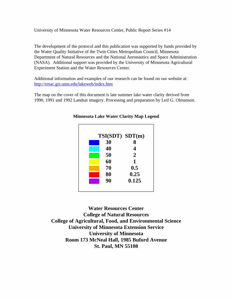
University of Minnesota Water Resources Center, Public Report Series #14 The development of the protocol and this publication was supported by funds provided by the Water Quality Initiative of the Twin Cities Metropolitan Council, Minnesota Department of Natural Resources and the National Aeronautics and Space Administration (NASA). Additional support was provided by the University of Minnesota Agricultural Experiment Station and the Water Resources Center. Additional information and examples of our research can be found on our website at: http://resac.gis.umn.edu/lakeweb/index.htm The map on the cover of this document is late summer lake water clarity derived from 1990, 1991 and 1992 Landsat imagery. Processing and preparation by Leif G. Olmanson.

Minnesota Lake Water Clarity Map Legend

Water Resources Center

College of Natural Resources College of Agricultural, Food, and Environmental Science

University of Minnesota Extension Service University of Minnesota

Room 173 McNeal Hall, 1985 Buford Avenue St. Paul, MN 55108

TSI(SDT)30405060708090

SDT(m)

0.1250.250.51248

Contents 1. Introduction ................................................................................................................ 1 2. Lake Reference Data ................................................................................................... 1 3. Hardware, Software and Images .................................................................................. 3

3.1 Hardware............................................................................................................... 3 3.2 Software................................................................................................................ 3 3.3 Satellite Image Data............................................................................................... 3

4. Classification Process .................................................................................................. 4 4.1 Image Pre-Processing ............................................................................................ 4 4.2 Water-Only Image ................................................................................................. 4 4.3 Unsupervised Classification of Water-Only Image.................................................. 5 4.4 Signature Acquisition............................................................................................. 7 4.5 Multiple Regression ............................................................................................. 10 4.6 Lake water clarity/trophic condition map ............................................................. 11

5. Conclusions............................................................................................................... 12

Figures

Figure 1. Normalized mean brightness values from unsupervised classification map.......... 6 Figure 2. September 4, 1991 unsupervised classification lake map used as a guide to avoid

vegetation and other effects when selecting area of interest locations. ...................... 6 Figure 3. AOI selection in ERDAS Imagine. .................................................................... 8 Figure 4. Pixel-level lake clarity map for Lake Minnetonka area (Hennepin Co. MN). ........ 11 Figure 5. September 4, 1991 lake-level water clarity/trophic condition map for lakes in

the Twin Cities Metropolitan Area, Minnesota, USA. ............................................ 12

Appendix

User’s Notes for Get_Hist (version 5)

1

1. Introduction This report describes methods for applying Landsat imagery to regional-scale assessment of lake water quality. The methods were developed from work initiated by Olmanson (1997) and continued in three subsequent studies conducted by the University of Minnesota Water Resources Center and Remote Sensing Laboratory: (1) a multi-year regional-scale lake water quality assessment of the seven-county Twin Cities Metropolitan Area (TCMA) funded by the Water Quality Initiative of the Twin Cities Metropolitan Council, (2) a study of cumulative impacts of land development on lakes in the north-central hardwood forest ecoregion funded by the Minnesota Department of Natural Resources and (3) a regional (Minnesota, Wisconsin and Michigan) assessment of lake clarity conducted as part of the Upper Midwest Regional Earth Science Applications Center (RESAC) funded by the NASA Earth Science Applications Program. This protocol is intended as a technical guide for image-processing analysts working on regional lake water clarity mapping. The image processing procedures were developed for Minnesota, but with appropriate modifications to reflect local programmatic interests and pre-existing geographic information and other data sources these procedures should work equally well for other regions. They are currently being used for classification of lakes in Minnesota, Wisconsin and Michigan. Because the protocol is written for image analysts performing image classification, as well as others involved in similar projects, it focuses on “how-to” technical procedures for image processing and includes references to specific ERDAS Imagine and ArcView commands and processes.

2. Lake Reference Data The principal objective is to perform regional assessments of lake water quality, in particular to estimate variables related to key management indicators, such as the trophic state indices of Carlson (1977). The three water quality variables that have been most commonly used to indicate trophic state are total phosphorus (TP), chlorophyll-a (Chl), and Secchi disk transparency (SDT) depth. Measurements of these water quality variables, along with various transformations such as the trophic state indices (TSIs), have been widely used by lake management agencies and organizations. Secchi disk transparency, a measure of water clarity, is strongly related to satellite spectral-radiometric observations of lakes. For lakes whose clarity is dominated by phytoplankton abundance, chlorophyll will be highly correlated with the satellite observations. Because phosphorus is the limiting nutrient for most lakes, it is generally correlated to chlorophyll in multi-lake analyses. However, phosphorus is not directly measurable by optical instruments such as the Landsat Thematic Mapper, and there are enough exceptions and deviations in the relationships between phosphorus, chlorophyll-a,

2

and SDT that we do not recommend estimating TP values for lakes from Landsat imagery at this time. The availability of lake reference data varies both over time and space in most study areas. Ideally, there should be at least 20 ground observation points for each image, and they should be distributed over a wide range of water quality/clarity. Contemporary studies usually can be designed to meet this criterion, but collecting the necessary ground observation data in remote areas may be difficult. In retrospective analyses, one must work within the confines of historical sampling programs. SDT measurements are the most consistently collected data and have been found to correlate well with Landsat data (Olmanson 1997, Kloiber et al. 2000). Because SDT measurements are inexpensive to collect and are conducive to volunteer monitoring programs, these measurements are collected on a regular basis throughout Minnesota and many other areas. For historical analyses, in situ water quality data can be acquired from local or state agencies or the U.S. Environmental Protection Agency's STORET national water-quality database. Information about STORET and available water quality data can be found at http://www.epa.gov/owow/storet/, or data can be requested by calling 1-800-424-9067. Reference data should be collected as close to the Landsat overpass date as possible. In the Twin Cities Metropolitan Area, where lake water clarity data are abundant, SDT measurements taken within one day of the Landsat overpass had somewhat better correlations with Landsat TM data than SDT measurements collected within seven days of the Landsat overpass (Kloiber et al. 2001). However, in more rural areas where fewer data are available, we have used data within 10 days of the Landsat overpass. Ideally reference data would be collected at the same time as the Landsat overpass and collected from a number of different lakes with varying water qualities. Most of our studies have calibrated Landsat TM data with ground-based SDT measurements and inferred SDT for all lakes in a Landsat image from the regression equation developed in the calibration step. The results then can be mapped directly as distributions of SDT in the lakes, or the estimated SDT values can be converted to Carlson’s (1977) trophic state index based on transparency TSI(SDT):

TSI(SDT) = 60 – 14.41 ln(SDT(m)) It is important to recognize that other factors aside from algal turbidity (as indicated by chlorophyll levels) may affect SDT in lakes. Most important of these (non-trophic-state) factors is humic color, but non-algal turbidity (e.g., soil-derived suspended sediment) also may be important in some lakes. For this reason, it is preferable to report Landsat results based on SDT calibrations directly as satellite-estimated SDT values or to use the explicit term, TSI(SDT), which identifies the value as an index based on transparency, rather than the generic term, TSI.

3

Because chlorophyll levels exhibit greater short-term variability within lakes than does SDT (Stadelmann et al. 2000), well-fitting predictive relationships probably will need to be based on ground-based measurements taken close in time (e.g., + 1-2 days) to the collection of a satellite image. This likely poses severe limitations on the use of historical data but should not be a major barrier in designing data collection efforts for current and future studies. Additional studies are necessary to develop an operational protocol for Landsat-based assessment of lake chlorophyll levels. In areas where in-situ data are not available, alternative methods for classification may need to be employed. These methods may include using data from an adjacent Landsat scene or from a different time period for the same scene to develop a regression relationship. Preliminary work on the latter method indicates that it is feasible as long as some method of radiometric calibration is applied. However, the resulting predictions from this method have a greater uncertainty than those obtained using in-situ data to develop a scene-specific regression relationship. Therefore, it is preferable to develop scene-specific relationships with in-situ data whenever possible. In the future, as better atmospheric correction technologies become available, other approaches may prove to be nearly as accurate.

3. Hardware, Software and Images 3.1 Hardware The computer platforms that we have used include Silicon Graphics Indigo workstations and Windows-based personal computers. With recent advances in computer hardware either system will work well. We recommend using the Windows NT or 2000 operating system on Pentium III computer or equivalent workstation with at least a 20 gigabyte hard drive and 128 megabytes of RAM. 3.2 Software The geographical information system (GIS) ArcView and ERDAS Imagine image (8.4) processing software were used in our work and are recommended for future studies. Other software packages such as PCI or ENVI could be used, but we did not evaluate them. 3.3 Satellite Image Data Satellite image data from a variety of sensors can be used for water quality assessment. We have had good success with Landsat TM and MSS imagery for regional assessments and with IKONOS for smaller city-scale assessments. Images selected for water quality assessment should be high-quality, cloud-free images selected from a late summer index period (July 15 - September 15, with a preference for August). This period was found to

4

be the best index period for remote sensing of water clarity in Minnesota (Kloiber et al. 2000; Stadelmann et al. 2001). There are at least two major advantages for using images from this period: (1) short-term variability in lake water clarity is at a seasonal minimum, and (2) most lakes have their minimum water clarity during this period. In addition, for trend analysis, it is preferable to have images from near anniversary dates. Landsat 5 and 7 images can be purchased for $600 from the United States Geological Surveys EROS Data Center, Sioux Falls, SD 57198 (http://edcwww.cr.usgs.gov/eros-home.html). IKONOS imagery can be purchased from Space Imaging (http://www.spaceimaging.com) for $13/km2 panchromatic and $13/km2 multispectral, with a minimum order of $3000.

4. Classification Process The image processing methods described below are designed to maximize the accuracy of the resulting lake classification. The classification process consists of a number of steps that are described in sections 4.1 through 4.6. 4.1 Image Pre-Processing The images should be registered to the Universal Transverse Mercator (UTM) projection system using the NAD 83 datum (or appropriate coordinate system for your area) and nearest neighbor resampling. Through careful selection of numerous (~40), well-defined, and well-distributed ground control points (GCPs), the positional accuracy (RMSE) should be on the order of ± 0.25 pixels, or 7.5 m. Images with RMSE values in excess of ± 1 pixel should be re-registered. We found that in Minnesota the Minnesota Department of Transportation highway map (available in ArcInfo GIS format) is an efficient and effective means of easily finding a large number of well-distributed GCPs. Atmospheric correction or normalization of the Landsat data is not necessary for the regression method described here, but would be necessary if in-situ data are not available for a particular image. 4.2 Water-Only Image A water-only image is created to reduce the file size of the Landsat image by removing unneeded data and to create a guide (unsupervised classification lake map) for development of an open-water image and selection of the area of interests (AOI) or sample locations. The water-only image also can be used to create a pixel-level lake condition map from the final regression model. To conserve file space, the run-length compression option should be used in ERDAS Imagine’s model-maker preferences for all image processing.

5

4.2.1 Unsupervised classification of the Landsat image: An unsupervised classification of the Landsat image is performed first to differentiate water from terrestrial areas. All seven Landsat bands are used for the classification, and ten classes should be specified. Because the spectral-radiometric response from water is significantly different from terrestrial features, water should be given its own, easily identifiable class or classes. 4.2.2 Mask terrestrial areas: Once the water class has been identified, the unsupervised classification map can be used as a binary mask to remove terrestrial areas from the original Landsat image. The resulting water-only image is used for further processing. 4.2.3 Cloud shadows, haze and other distortions: Once the water-only image has been created, it should be checked to determine whether cloud shadows, haze or other distortions such as image edge effects are included with the water pixels. If these effects are present, the affected areas should be cropped using an area of interest (AOI) and the subset option in ERDAS. An alternative or additional method uses an unsupervised classification of the water-only image to allow these effects to be differentiated from the water, and as above, they can be removed by masking. 4.3 Unsupervised Classification of Water-Only Image One of the most important steps when classifying lake water quality is acquiring a representative sample from each lake. Ideally the sample should represent the center portion of the lake in at least 15 feet of water (or twice the SDT measurement) where reflectance from vegetation, the shoreline, or the lake bottom will not affect the resulting spectral signature. An unsupervised classification of the water-only image is performed to differentiate water affected by varying concentrations of algae from water affected by vegetation, shoreline and/or bottom effects. This is achieved using the following steps: • Conduct an unsupervised classification of the water-only image using 10 classes. • In the Signature Editor open the water-only signature file and in (view/columns/statistics/) select “mean”,

then apply. Select “signature name, mean (layer 1) through mean (layer 7)” columns. Export the spectral signatures for the seven TM bands from this classification into a "dat" file.

• Import the file into a spreadsheet program and make a graph of the mean brightness measurement for each band. Normalize the data by subtracting the lowest mean brightness value for each band.

• Areas that have vegetation, shoreline and/or bottom effects can be inferred from signatures with elevated near infrared (band 4) and/or middle infrared (band 5) responses, as shown in Figure 1.

• Color code the map to identify the variations in water quality and highlight features that are affected by vegetation, shoreline and/or bottom effects. These areas should be avoided when acquiring samples. An example of an unsupervised classification lake map is presented as Figure 2.

• Review locations of pixels from the different affected classes and verify the inferred classification. Note that class 1 has elevated near infrared (band 4) and middle infrared (band 5) responses but occurs in deep water areas of clear lakes. Therefore, class 1 is not affected by vegetation, shoreline and/or bottom effects.

6

0

5

10

15

20

25

TM 1 TM 2 TM 3 TM 4 TM 5 TM 7

Landsat Band

Bri

ghtn

ess

Class 1Class 2Class 3Class 4Class 5Class 6Class 7Class 8Class 9Class 10

Figure 1. Normalized mean brightness values from unsupervised classification map.

Figure 2. September 4, 1991 unsupervised classification lake map used as a guide to avoid vegetation and other effects when selecting area of interest locations.

7

4.4 Signature Acquisition Another important issue is to determine what lakes to acquire spectral radiometric data from. If the goal is to simply create a pixel-level water clarity map, then data need to be acquired only from those lakes with reference data which will be use to develop a water clarity model. However, if the desired output is to develop a database of water clarity for all lakes of a certain criteria, then samples need to be acquired from all lakes of interest. This approach gives a water clarity (SDT) value for each lake and has the advantage of enabling one to use the data in other studies while also allowing the creation of lake-level or pixel-level water clarity or trophic condition maps. In Minnesota we acquired spectral radiometric data from all open water lakes that were � 20 acres and from lakes < 20 acres if reference water clarity data were available for the lake. To avoid vegetation, shoreline and bottom effects lake bathymetric maps, if available, and an unsupervised classification of the water-only image (discussed in 4.3) can be used as guides when selecting area of interest (AOI) locations. Both provide important information regarding pixels that may be affected by these interference factors. 4.4.1 AOI signature acquisition method: Open two viewers in ERDAS Imagine. Open the water-only image in one of the viewers and the unsupervised classification of the water-only image in the other. Link the viewers. With the AOI tool select AOI locations in the water-only viewer that best represent each lake while avoiding areas that may be affected by vegetation, shoreline and/or bottom effects, as shown in Figure 3. For best results, AOIs should contain at least eight pixels in smaller lakes and may be up to 1000 pixels in size in larger lakes (Kloiber et al. 2001). This approach allows for a larger sample while avoiding areas with differing transparencies and areas affected by vegetation or bottom effects. Larger samples such as the interior sample method evaluated by Lillesand et al. (1983) were determined to have the best correlation with reference data due to the smoothing of radiometric noise. More than one AOI may be needed in complex lake systems with multiple bays. Once the AOI location has been selected, a signature can be acquired from the AOI in the Signature Editor and labeled with the appropriate lake identification number. This can be done in the following steps: • Select AOI location. • In the Signature Editor select, create new signatures from AOI. Label with appropriate lake identification

number. Repeat until all lake signatures have been acquired. • In the Signature Editor (view/columns/statistics/) select “mean”, then apply. Select “signature name, count

and mean (layer 1) through mean (layer 7) columns”. Export the columns into a “dat” file for subsequent analysis.

8

Figure 3. AOI selection in ERDAS Imagine.

4.4.2 Alternative signature acquisition method: A more efficient approach to use when there are a large number of lakes, or when samples are being acquired from the same lakes from a number of different images is to use the modified histogram method. The modified histogram method uses the lake polygons to extract data from all unaffected water pixels. The “GetHist” program (Appendix) then is used to calculate the mean of the darkest specified percent of each bands radiometric histogram. This method has given results similar to the AOI method and can be more efficient for some studies. The use of this method depends on a good quality lake polygon layer that has unique lake identification numbers for all lakes and sub-basins. The modified histogram method is described in more detail in sections 4.4.2.1 through 4.4.2.3.

9

4.4.2.1 Create the study lakes polygon coverage: The exact procedure to create this coverage may vary with the availability of GIS coverages. In Minnesota we used a tagged (DOW lake number) GIS surface hydrography coverage linked with the DNR Waters Lake List as the basis for the lakes polygon coverage. The basic steps used to create this coverage in ArcView are: • Create polygon coverage of lakes from surface hydrography layer (remove non-lake features). • Link DNR Lake List with lake attributes to lake polygon coverage using the unique lake identification (ID)

number as the “join field” and save as a new lakes polygon coverage. • Edit lake polygon coverage as necessary. If lake area attribute is not already present in the lake coverage,

create it in ArcView by adding a numeric field. Using the field calculator, submit the following request "[Shape].ReturnArea" followed by the appropriate units conversion to convert square map units into acres.

• Select lakes of interest (� 20 acres) and create study lakes coverage from the selected lake fe atures. Verify that all study lakes have the appropriate unique lake ID number. Add lake ID numbers if necessary. Lakes with sub-basins need to be split and identified with unique lake sub-basin identification.

4.4.2.2 Open water image: To avoid vegetation, shoreline and bottom effects, the unsupervised classification of the water-only image (discussed in 4.3) is used as a binary mask to remove affected pixels from the water-only image. In the example above class 7, class 8, class 9, and class 10 are masked. The resulting open water image is used for further processing. 4.4.2.3 Extract lake signatures in ERDAS Imagine: • Open a Viewer. • In the Viewer, choose File/Open/Raster Layer and open the Open Water image. • In the same Viewer, choose File/Open/Vector Layer and open the study lakes coverage. • Choose Vector/Viewing Properties. In the Properties dialog box, deselect “Arcs” and select “Polygon” to

display polygons (the default is to display vectors as arcs). Click “Apply” and then “Close”. • Choose Vector/Tools. Use the selection rectangle tool to select all lake polygons that are included in the

Open Water image. • Choose AOI/Copy Selection to AOI. An AOI coverage will be created with the same polygons from the

vector coverage. If there are many polygons in the vector coverage, this can take a while. • Choose File/Save/AOI Layer to save the AOI layer. • While the polygons are still selected, choose Vector/Attributes. In the Attributes dialog box, select the

column containing unique lake names or DNR lake ID codes. Right click in the gray panel at the top of this column for column properties, and choose “Export”. Save the lake ID column to a text file. Close the Attributes dialog box.

• Open a Signature Editor. • In the Viewer, choose AOI/Tools. Use the selection rectangle tool to select all lake AOIs. • In the Signature Editor, create new signatures from AOIs. If there are many lake AOIs, this can take a

while. • In the Signature Editor, choose File/Report. Check “Histograms” and “All Signatures”. • When the report appears in a text editor window, choose File/Save As.

10

4.4.2.4 Processing histogram data and importing into a spreadsheet: • Run the program GetHist.exe. • Select ignore zeros. • Choose the percentage of the histogram to include (when using the Open Water image we have found that

50 percent works well). • Select bottom N% (the darkest pixels). Note these selections must be made before proceeding to the next

step. • Click on “Read Histograms from Text File”, and choose the signature report you created in 4.4.2.3 above.

The GetHist window should show the number of signatures (n) and the number of spectral bands (b) for each signature.

• Click on “Save Statistics” to save the data to a comma-delimited text file, then “Exit”. • Import the comma-delimited text file into a spreadsheet (e.g., Microsoft Excel).

Signature: will be the signature number (0 to n-1). Total Pixel: will be the total number of pixels in the original signature, including zeros. Error Flag: will identify signatures that used less than one pixel to calculate the signature. B [b] Mean: The mean of the selected portion of the histogram, for band b. B [b] Count: The number of pixels used to compute this mean, for band b.

• Import the text file with DNR lake ID numbers into the spreadsheet. The lake ID numbers and the histogram statistics should be in the same order.

• Copy DNR lake ID numbers column. • Paste to signature column. • Make sure DNR lake ID numbers line up with the right lake signature (this can be done to a degree by

verifying the number of pixels). • Edit spreadsheet to removing flagged signatures and signatures when fewer than 8 pixels were used to

calculate the mean. • Edit spreadsheet to remove multiple signatures for a given lake identification number. Lakes with more

than one polygon for a given lake either need to be given unique identification sub-basin numbers for each polygon. The signature that best represents the lake (usually the signature with the largest number of pixels) should be selected, and the remaining signatures should be removed.

• Review original Landsat image and identify any lakes that have cloud shadows or haze. The signatures extracted from these lakes will be affected by the cloud shadows or haze and should not be used. If a lake is only partially affected an AOI lake sample (which was described in section 4.4.1) can be acquired from an unaffected area.

4.5 Multiple Regression In initial studies we used a reverse stepwise regression to find the bands that were significant, followed by a complete, multiple regression for only the significant bands to determine the relationship for each image. For routine application of the procedure on a regional scale, the same band combinations should be used over time to facilitate comparability of results. Based on results from Klobier et al. (2001), we recommend using the TM1:TM3 ratio, along with TM1 for the lake water clarity regression model. The TM1:TM3 ratio was the most significant factor for all ten images analyzed, accounting for most of the variability in observed lake water clarity. The TM1 variable improved the regression relationship slightly. This analysis also found that a semi-log relationship between the mean brightness values of the Landsat TM bands for the AOIs and the log of SDT met the basic assumptions for the regression model for all ten images analyzed. The basic steps of the regression analysis are outlined below.

11

• Import the text signature file generated in step 4.4.1 or 4.4.2.4 into a spreadsheet such as Microsoft Excel. • Input all available SDT data within a specified time 1-2 days of the image date into the spreadsheet or

create a new SDT spreadsheet. • Import the two spreadsheets into a database tool, such as Microsoft Access. Perform a table join

between the two data sets using the unique lake ID number as the “join field.” • Export the results of the “table join” to a format that can be imported into a statistical analysis software

package (tab delimited text, DBF, or Excel formats are fairly common). • Import the data into a statistical analysis package. • Perform a natural log transformation on SDT and calculate the TM1:TM3 ratio. • Run a complete multiple regression analysis with ln(SDT) as the dependent variable and TM1:TM3 ratio

and TM1 as independent variables . • Review the R2, standard error, outlier report and residual plot. Our studies have found R2 = ~ 0.8 and

standard error = ~ 0.3 for images within the index period (July 15 – September 15). • Evaluate any statistical outliers, if present. If the data seem obviously biased or if there is possible

interference in the satellite data, the outlier should be removed. Outlier removal is a matter of professional judgement and is discussed in basic statistical reference books.

• After screening the relationship for outliers and removing any of these, if appropriate, the regression model should be re-run to produce the final regression model equation.

4.6 Lake water clarity/trophic condition map With the relationship that was determined in section 4.5, lake water clarity or trophic condition maps can be created using one of two methods. The first method uses the ERDAS modeler to create a pixel-level lake map. With this map all water pixels will be classified and intra-lake differences can be evaluated. An example of a pixel-level water clarity/trophic condition map for the Lake Minnetonka area (Hennepin County, Minnesota) is presented in Figure 4.

N

EW

S

(SDT)

30405060708090

(m)

0.1250.250.51248

TSI SDT

1 0 1 Miles

Figure 4. Pixel-level lake clarity map for Lake Minnetonka area (Hennepin Co. MN).

12

The other method uses ArcView to create a lake-level water clarity or trophic condition map. An example of a lake-level water clarity/trophic condition map for the TCMA is presented in Figure 5. This type of map can be created using the following steps: • Using the final regression equation, calculate Landsat-estimated SDT or the log-transformed index,

TSI(SDT), in the reformatted signature file created in step 4.5. • Import the results from the previous step into ArcView and perform a table join to the study lake polygon

coverage using the unique lake ID number as the “join field”. • Use the ArcView Legend Editor to create a lake water clarity (SDT) or TSI(SDT) map by selecting the

graduated color legend type and using the estimated clarity (SDT in m) or TSI(SDT) field as the classification field. Figure 4 or 5 may be used as a guide for developing the legend.

N

EW

S

(SDT)30405060708090

(m)

0.1250.250.51248

TSI SDT

5 0 5 Miles

Figure 5. September 4, 1991 lake-level water clarity/trophic condition map for lakes in the Twin Cities Metropolitan Area, Minnesota, USA.

5. Conclusions This document describes the image processing procedures we used for a multi-year (1973-1998) assessment of over 500 lakes in the Twin Cities Metropolitan Area, as well as for statewide classification of over 10,000 lakes in Minnesota. We expect that the techniques will evolve and improve as new data sources and methods become available, but believe that this document provides an objective and repeatable approach for classification of lake clarity.

13

References Carlson, R.E. 1977. A trophic state index for lakes. Limnology and Oceanography. 22(2):p 361-369. Kloiber, S.M., T. Anderle, P.L. Brezonik, L.G. Olmanson, M.E. Bauer, and D.A. Brown. 2000. Trophic state assessment of lakes in the Twin Cities (Minnesota, USA) region by satellite imagery. Arch. Hydrobiol. Ergebn. Limnol. 55:p 137-151. Kloiber, S.M., Brezonik, P.L., Olmanson, L.G., and Bauer, M.E, 2001. Development of a remote sensing method for synoptic, regional water quality assessment. Remote Sens. Environ. (in review). Lillesand, T.M., W.L. Johnson, R.L. Deuell, O.M. Lindstrom, and D.E. Meisner. 1983. Use of Landsat data to predict the trophic state of Minnesota Lakes. Photogramm. Eng. Remote Sens. 49(2): 219-229. Olmanson, L.G. 1997. Satellite remote sensing of the trophic state conditions of the lakes in the Twin Cities metropolitan area. Masters paper, Water Resources Science Graduate Program, University of Minnesota, St. Paul, MN. Stadelmann, T.H., Brezonik, P.L., and Kloiber, S.M. 2001. Seasonal patterns of chlorophyll a and Secchi disk transparency in lakes of east-central Minnesota: implications for design of ground- and satellite-based monitoring programs. Lake Reserv. Manage. 17: (in press).

Acknowledgement Jonathan W. Chipman, Environmental Remote Sensing Center, Institute for Environmental Studies, University of Wisconsin-Madison – For development of the “GetHist” program.

Appendix

User’s Notes for Get_Hist (version 5)

Jonathan W. Chipman Environmental Remote Sensing Center

Institute for Environmental Studies University of Wisconsin-Madison

About Get_Hist The GetHist program will read an ASCII text report generated by the ERDAS Imagine Signature Editor, perform various calculations, and write the results out to a comma-delimited text file suitable for use with Microsoft Excel or any similar spreadsheet. The calculations that Get_Hist performs involve finding the mean of a particular user-specified portion of the histograms in one or more spectral bands, for one or more spectral signatures. Please address questions regarding Get_Hist to Jonathan W. Chipman, by email at jchipman@students.wisc.edu or by phone at the Environmental Remote Sensing Center, 608-263-6584 or 608-262-1585.

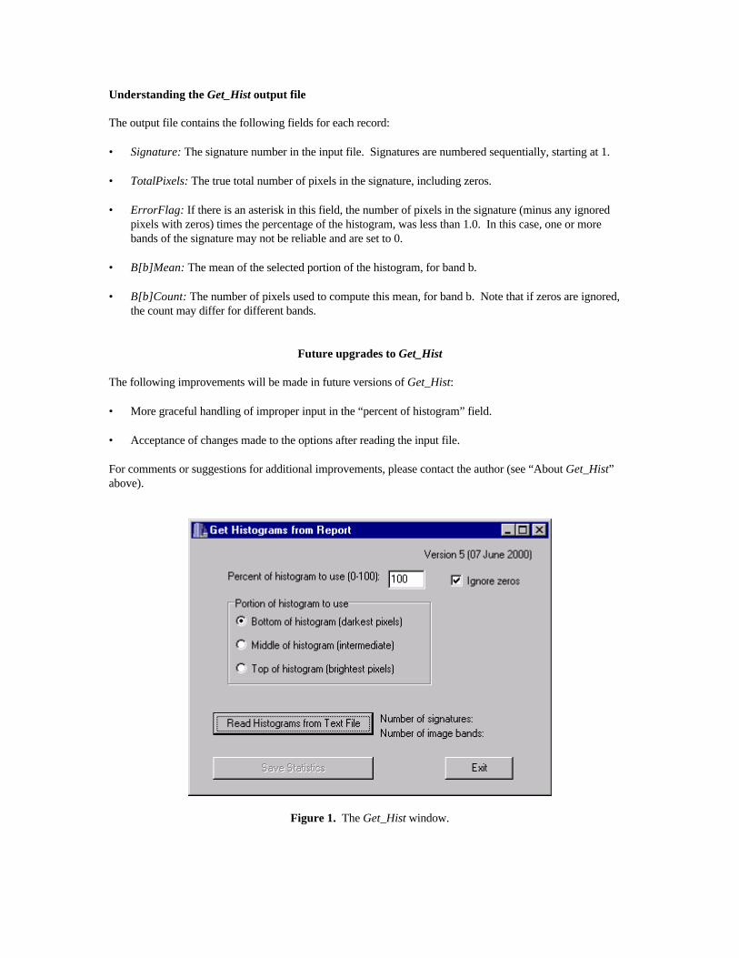
Compatibility The format of the report files generated by the Imagine Signature Editor is slightly different in Imagine v. 8.3 and v. 8.4. Get_Hist is compatible with both formats. The output file generated by Get_Hist is an ASCII text file with comma-delimited fields. The first record contains the field names. This format should be usable with Microsoft Excel or any similar spreadsheet software. Running Get_Hist The Get_Hist window is shown in Figure 1. There are three options that must be set before reading the input file: • Ignore zeros: If this box is checked, Get_Hist will ignore any zeros in the histogram. • Percentage of histogram to use (0-100): This specifies the percentage of the histogram that will be used,

minus any “ignored” pixels (see above). Numbers below 0 will be set to 0%, and numbers above 100 will be set to 100%. Any non-numeric characters in this field may cause Get_Hist to become unhappy (this should be changed in a future version).

• Portion of histogram to use: There are three choices – use the bottom N% of the histogram (the darkest

pixels), the middle N% of the histogram, or the upper N% of the histogram (the brightest pixels). Choosing the middle N% will have the effect of excluding the two tails of the histogram, each tail having [(100-N)/2]% of the histogram.

Be sure to set all three options before reading the input file. Changes made to the options after reading the input file will not be reflected in the output file (this should be changed in a future version).

Understanding the Get_Hist output file The output file contains the following fields for each record: • Signature: The signature number in the input file. Signatures are numbered sequentially, starting at 1. • TotalPixels: The true total number of pixels in the signature, including zeros. • ErrorFlag: If there is an asterisk in this field, the number of pixels in the signature (minus any ignored

pixels with zeros) times the percentage of the histogram, was less than 1.0. In this case, one or more bands of the signature may not be reliable and are set to 0.

• B[b]Mean: The mean of the selected portion of the histogram, for band b. • B[b]Count: The number of pixels used to compute this mean, for band b. Note that if zeros are ignored,

the count may differ for different bands.

Future upgrades to Get_Hist The following improvements will be made in future versions of Get_Hist: • More graceful handling of improper input in the “percent of histogram” field. • Acceptance of changes made to the options after reading the input file. For comments or suggestions for additional improvements, please contact the author (see “About Get_Hist” above).

Figure 1. The Get_Hist window.