Image Processing Compression and Reconstruction by Using New Approach Artificial Neural Network

K.Siva Nagi Reddy, Dr.B.R.Vikram, L.Koteswara Rao, B.Sudheer Reddy

International Journal of Image Processing (IJIP), Volume (6) : Issue (2) : 2012 68

Image Compression and Reconstruction Using a New Approach by Artificial Neural Network

K.Siva Nagi Reddy [email protected] Associate Professor, Dept of ECE, Montessori Siva Sivani Institute of Science and Technology, College of Engineering, Mylavaram, Vijayawada, Andhra Pradesh, INDIA.

Dr.B.R.Vikram [email protected] Professor, Dept of ECE, Vijay Rural Engineering College, Nizamabad, Nizamabad (D.t), Andhra- Pradesh, INDIA.

L. Koteswara Rao [email protected] Asst. Professor, Dept of ECE, Faculty of Science & Technology, IFHE (University), Hyderabad, India

B.Sudheer Reddy [email protected] Associate Professor, Dept of CSE, Montessori Siva Sivani Institute of Science and Technology, College of Engineering, Mylavaram, Vijayawada, Andhra Pradesh, INDIA.

Abstract

In this paper a neural network based image compression method is presented. Neural networks offer the potential for providing a novel solution to the problem of data compression by its ability to generate an internal data representation. This network, which is an application of back propagation network, accepts a large amount of image data, compresses it for storage or transmission, and subsequently restores it when desired. A new approach for reducing training time by reconstructing representative vectors has also been proposed. Performance of the network has been evaluated using some standard real world images. It is shown that the development architecture and training algorithm provide high compression ratio and low distortion while maintaining the ability to generalize and is very robust as well.

Key words: Artificial Neural Network, Image Processing (ANN), Multilayer Perception (MLP) and Radial Basis Functions (RBF),Normalization, Levenberg-Marquardt, Jacobian

1. INTRODUCTION Artificial Neural networks are simplified models of the biological neuron system and therefore have drawn their motivation from the computing performed by a human brain. A neural network, in general, is a highly interconnected network of a large number of processing elements called neurons in an architecture inspired by the brain. Artificial neural networks are massively parallel adaptive networks of simple nonlinear computing elements called neurons which are intended to abstract and model some of the functionality of the human nervous system in an attempt to partially capture some of its computational strengths. A neural network can be viewed as comprising eight components which are neurons, activation state vector, signal function, pattern of connectivity, activity aggregation rule, activation rule, learning rule and environment.



Recently, artificial neural networks [1] are increasingly being examined and considered as possible solutions to problems and for application in many fields where high computation rates are required [2]. Many People have proposed several kinds of image compression methods [3]. Using Artificial neural network (ANN) technique with various ways [4, 5, 6, 7]. A detail survey of about how ANN can be applied for compression purpose is reported in [8,9,10,11].Broadly, two different categories for improving the compression methods and performance have been suggested. Firstly, develop the existence method of compression by use of ANN technology so that improvement in the design of existing method can be achieved. Secondly, apply neural network to develop the compression scheme itself, so that new methods can be developed and further research and possibilities can be explored for future. The typical image compression methods are based on BPNN techniques. The Back propagation Neural Network (BPNN) is the most widely used multi layer feed forward ANN. The BPNN consists of three or more fully interconnected layers of neurons. The BP training can be applied to any multilayer NN that uses differentiable activation function and supervised training [12].

The BPNN has the simplest architecture of ANN that has been developed for image compression but its drawback is very slow convergence. In [13] suggested mapping the gray levels of the image pixels and their neighbors in such a way that the difference in gray levels of the neighbors with the pixel is minimized and then the CR and network convergence can be improved. They achieved this by estimating a Cumulative Distribution Function (CDF) for the image. They used CDF to map the image pixels, then, the BPNN yields high CR and converges quickly. In [14] used BPNN for image compression and developed algorithm based on improved BP. The blocks of original image are classified into three classes: background blocks, object blocks and edge blocks, considering the features of intensity change and visual discrimination Finally, In [15] presented an adaptive method based on BPNN for image compression/decompression based on complexity level of the image by dividing image into blocks, computing the complexity of each block and then selecting one network for each block according to its complexity value. They used three complexity measure methods such as: entropy, activity and pattern-based to determine the level of complexity in image blocks. This paper is organized as follows. In section II we discuss Methodology (Image compression using ANN) III Describes the Neural network models. IV Describes the multi-layer perception neural network and its approach that is directly developed for image compression. In section V describe the Process steps for compression. VI explains the experimental results of our implementation are discussed and finally in section VII we conclude this research and give a summary on it.

2. METHODOLOGY (IMAGE COMPRESSION USING ANN) 2.1 Introduction to Image Compression Image Processing is a very interesting and a hot area where day-to-day improvement is quite inexplicable and has become an integral part of own lives. Image processing is the analysis, manipulation, storage, and display of graphical images. An image is digitized to convert it to a form which can be stored in a computer's memory or on some form of storage media such as a hard disk. This digitization procedure can be done by a scanner, or by a video camera connected to a frame grabber board in a computer. Once the image has been digitized, it can be operated upon by various image processing operations. Image processing is a module that is primarily used to enhance the quality and appearance of black and white images. It also enhances the quality of the scanned or faxed document, by performing operations that remove imperfections. Image processing operations can be roughly divided into three major categories, Image Enhancement, Image Restoration and Image Compression. Image compression is familiar to most people. It involves reducing the amount of memory needed to store a digital image.



Digital image presentation requires a large amount of data and its transmission over communication channels is time consuming. To rectify that problem , large number of techniques to compress the amount of data for representing a digital image have been developed to make its storage and transmission economical. One of the major difficulties encountered in image processing is the huge amount of data used to store an image. Thus, there is a pressing need to limit the resulting data volume. Image compression techniques aim to remove the redundancy present in data in a way, which makes image reconstruction possible. Image compression continues to be an important subject in many areas such as communication, data storage, computation etc. In order to achieve useful compression various algorithms were developed in past. A compression algorithm has a corresponding decompression algorithm that, given the compressed file, reproduces the original file. There have been many types of compression algorithms developed. These algorithms fall into two broad types, 1) Loss less algorithms, and 2) Lossy algorithms. A lossless algorithm reproduces the original exactly. Whereas, a lossy algorithm, as its name implies, loses some data. Data loss may be unacceptable in many applications. For example, text compression must be lossless because a very small difference can result in statements with totally different meanings. There are also many situations where loss may be either Unnoticeable or acceptable. But various applications require accurate retrieval of image, wherein one such application is medical processing. So Image Compression enhances the progress of the world in communication.

2.2 NETWORK Selection for Compression (Back propagation) The first step to solve the problem is to find the size of the network that will perform the desired data compression. We would like to select a network architecture that provides a reasonable data reduction factor while still enabling us to recover a close approximation of the original image from the encoded form. This network used is a feed forward network consists of three layers, one Input Layer (IL) with N neurons, one Output Layer (OL) with N neurons and one (or more) Hidden Layer (HL) with Y neurons. All connections are from units in one layer to the other. The hidden layer consists of fewer units than the input layer, thus compress the image. The size of the output and the input layer is same and is used to recover the compressed image. The network is trained using a training set of patterns with desired outputs being same as the inputs using back propagation of error measures. Using the back-propagation process the network will develop the internal weight coding so that the image is compressed for ratio of number of input layer nodes to the number of hidden layer nodes equal to four. If we then read out the values produced by the hidden layer units in our network and transmit those values to our receiving station, we can reconstruct the original image by propagating the compressed image to the output units in identical networks. The number of connections between each two layers in NN is calculated by multiplying the total number of neurons of the two layers, then adding the number of bias neurons connections of the second layer (bias connections of a layer is equal to the number of layer neurons). If there are Ni neurons in the input layer, Nh neurons in the hidden layer and No neurons in the output layer, the total number of connections is given by equation:

Network Size:(Nw)= [(Ni*Nh)+Nh]+[(Nh*No)+No]



FIGURE 1: Neural Networks Architecture

2.3 IMAGE PRE-PROCESSING 2.3.1 RGB to Y Cb Cr and back to RGB.

The Y, Cb, and Cr components of one color image are defined in YUV color coordinate, where Y is commonly called the luminance and Cb, Cr are commonly called the chrominance. The meaning of luminance and chrominance is described as follows

� Luminance: received brightness of the light, which is proportional to the total energy in the visible band.

� Chrominance: describe the perceived color tone of a light, which depends on the wavelength composition of light chrominance is in turn characterized by two attributes – hue and saturation.

1. hue: Specify the color tone, which depends on the peak wavelength of the light 2. saturation: Describe how pure the color is, which depends on the spread or bandwidth of

the light spectrum 3.

The RGB primary commonly used for color display mixes the luminance and chrominance attributes of a light. In many applications, it is desirable to describe a color in terms of its luminance and chrominance content separately, to enable more efficient processing and transmission of color signals. Towards this goal, various three-component color coordinates have been developed, in which one component reflects the luminance and the other two collectively characterize hue and saturation. One such coordinate is the YUV color space. The [Y Cb Cr]

T

values in the YUV coordinate are related to the [R G B]T values in the RGB coordinate by

+

−−

−−=

128

128

16

071.0368.0439.0

439.0291.0148.0

098.0504.0257.0

B

G

R

Cr

Cb

Y

−

−

−

−−=

128

128

16

000.0017.2164.1

813.0392.0164.1

596.1000.0164.1

Cr

Cb

Y

B

G

R

FIGURE 2: Color conversion matrices for RGB and Y Cb Cr



Similarly, if we would like to transform the YUV coordinate back to RGB coordinate, the inverse matrix can be calculated from (1.1), and the inverse transform is taken to obtain the corresponding RGB components. 2.3.2 Spatial Sampling of Color Component

FIGURE 3: Three different chrominance down sampling format

Because the eyes of human are more sensitive to the luminance than the chrominance, the sampling rate of chrominance components is half that of the luminance component. This will result in good performance in image compression with almost no loss of characteristics in visual perception of the new up sampled image. There are three color formats in the baseline system: � 4:4:4 formats: The sampling rate of the luminance component is the same as those of the chrominance. � 4:2:2 formats: There are 2 Cb samples and 2 Cr samples for every 4 Y samples. This leads to half number of pixels in each line, but the same number of lines per frame. � 4:2:0 formats: Sample the Cb and Cr components by half in both the horizontal and vertical directions. In this format, there are also 1 Cb sample and 1 Cr sample for every 4 Y samples.

At the decoder, the down sampled chrominance components of 4:2:2 and 4:2:0 formats should be up sampled back to 4:4:4 formats.

2.3.3 Image Normalization and Segmentation The image data is represented by the pixel value function f(X,Y) where X and Y correspond to the spatial coordinates within the image with pixel values between 0 and 2k-1, where k is the number of bits which represent each pixel in the image, usually k = 8, then the pixel values would lie within the range [0-255]. The ANN requires inputs with real type and the sigmoid function of each ANN neuron requires the input data to be in the range [0-1]. For this reason the image data values must be normalized. The normalization is the process of linearly transformation of image values from the range [0-255] into another range that is appropriate for ANN requirements to obtain valuable results and to speed up the learning .In this paper, the image is linearly transformed from range [0-255] to range [0-1]. Image segmentation is the process of dividing the image into sub images, each of which is considered to be a new separate image. In this paper, the image is segmented by dividing it into non overlapping blocks with equal size to simplify the learning/compressing processes. The input layer units of ANN are represented by one-dimensional vector. Image rasterization is the process of converting each sub image from a two-dimensional block in to a one dimensional vector. 2.4 Initialization of ANN Learning Parameters The weight connections of the ANN are represented by two weight matrices. The first matrix is V which represents the weight connections between the input and hidden layer units and the second matrix is W which represents the weight connections between the hidden and output layer



units. These two weight matrices must be initialized to small random numbers because the network may be saturated by large values of the weights. The learning rate value usually reflects the rate of network learning and its value (between 0.1 and 0.9) is chosen by the user of the network. Values that are very large can lead to instability in the network and unsatisfactory learning, while values that are too small can lead to excessively slow learning. 2.5 Training the ANN The input image is split up into blocks or vectors of 4×4, 8 ×8 or 16×16 pixels. These vectors are used as inputs to the network. The network is provide by the expected (or the desired) output, and it is trained so that the coupling weights, {wij}, scale the input vector of N -dimension into a narrow channel of Y -dimension (Y < N) at the hidden layer and produce the optimum output value which makes the quadratic error between output and the desired one minimum. In fact this part represents the learning phase, where the network will learn how to perform the task. In this process of leering a training algorithm is used to update network weights by comparing the result that was obtained and the results that was expected. It then uses this information to systematically modify the weight throughout the network till it finds the optimum weights matrix.

FIGURE 4: Block diagram of ANN training

2.6 Encoding The trained network is now ready to be used for image compression which, is achieved by dividing or input images into normalization and segmentation. The segmented image blocks to rasterization and that vector is given to input layer then the output of hidden layer renormalized to represent the compressed image.

FIGURE 5: Block diagram of the Encoding Steps

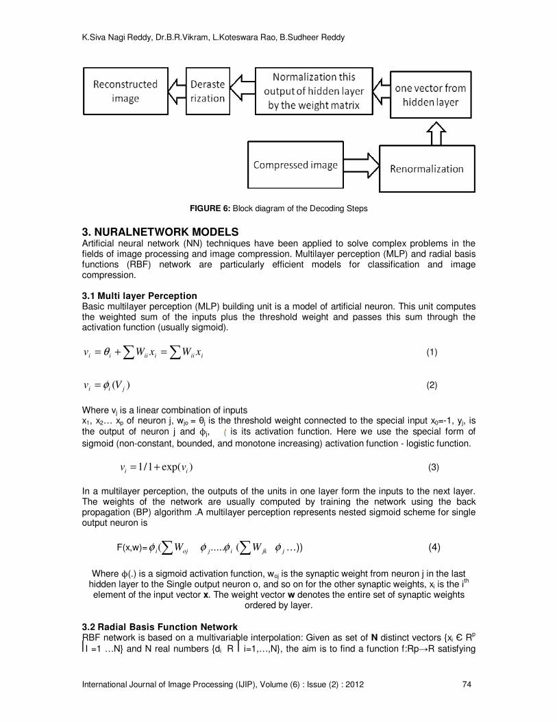
2.7 Decoding To decompress the image; first the compressed image is renormalized then applies it to the output of the hidden layer and get the one vector of the hidden layer output is normalized then it rasterization to represent the reconstruct the image. Fig. 6 show the decoder block diagram.



FIGURE 6: Block diagram of the Decoding Steps

3. NURALNETWORK MODELS Artificial neural network (NN) techniques have been applied to solve complex problems in the fields of image processing and image compression. Multilayer perception (MLP) and radial basis functions (RBF) network are particularly efficient models for classification and image compression. 3.1 Multi layer Perception Basic multilayer perception (MLP) building unit is a model of artificial neuron. This unit computes the weighted sum of the inputs plus the threshold weight and passes this sum through the activation function (usually sigmoid).

iiiiiiii xWxWv ∑∑ =+= θ (1)

)( jii Vv φ= (2)

Where vj is a linear combination of inputs x1, x2… xp of neuron j, wjo = θj is the threshold weight connected to the special input x0=-1, yj, is the output of neuron j and ϕj, is its activation function. Here we use the special form of

sigmoid (non-constant, bounded, and monotone increasing) activation function - logistic function.

)exp(1/1ii

vv += (3)

In a multilayer perception, the outputs of the units in one layer form the inputs to the next layer. The weights of the network are usually computed by training the network using the back propagation (BP) algorithm .A multilayer perception represents nested sigmoid scheme for single output neuron is

F(x,w)= ∑ oji W(φ ij φφ ..... ∑ jkW( jφ …)) (4)

Where ϕ(.) is a sigmoid activation function, woj is the synaptic weight from neuron j in the last

hidden layer to the Single output neuron o, and so on for the other synaptic weights, xi is the ith

element of the input vector x. The weight vector w denotes the entire set of synaptic weights ordered by layer.

3.2 Radial Basis Function Network RBF network is based on a multivariable interpolation: Given as set of N distinct vectors {xi Є R

p

⎢I =1 …N} and N real numbers {di R ⎜i=1,…,N}, the aim is to find a function f:Rp→R satisfying



the condition f(xi)= di, i=1, ,N. RBF approach works with N radial basis functions (RBF) Φj where

Φi: Rp→R, i=1, ,N and Φj = Φ (|| x- Ci ||), where Φ:R+→R, xi Є Rp, || || is a norm on Rp, Ci Rp

are centers of RBFs. Centers are set to Ci=xi Rp, i=1,…,N. Very often used form of RBF is the Gaussian function Φi (x)=exp(-x

2/2σ2), where σ is a width (parameter). Functions

F(x) = φ∑ iiW( (|| x-i

v ||) (5)

i=1,…,N form the basis of a liner space and interpolation function f is their linear combination Interpolation problem is simple to solve, in contrast to approximation problem (there is N given points and n0 functions Φ, where n0<N.), which is more complicated. Then it is a problem to set centers Ci i=1…n0, also parameter σ of each RBF can be not the same for all RBFs. One possible solution for RBF approximation problem is a neural network solution. RBF network is a feed forward network consisting of input, one hidden and output layer. Input layer distributes input vectors into the network, hidden layer represents RBFs Φ. The linear output neurons compute linear combinations of their inputs. The RBF model is suitable for data interpolation and classification. For this work, the RBF model was trained from the selected input vectors producing the synaptic weight vectors.

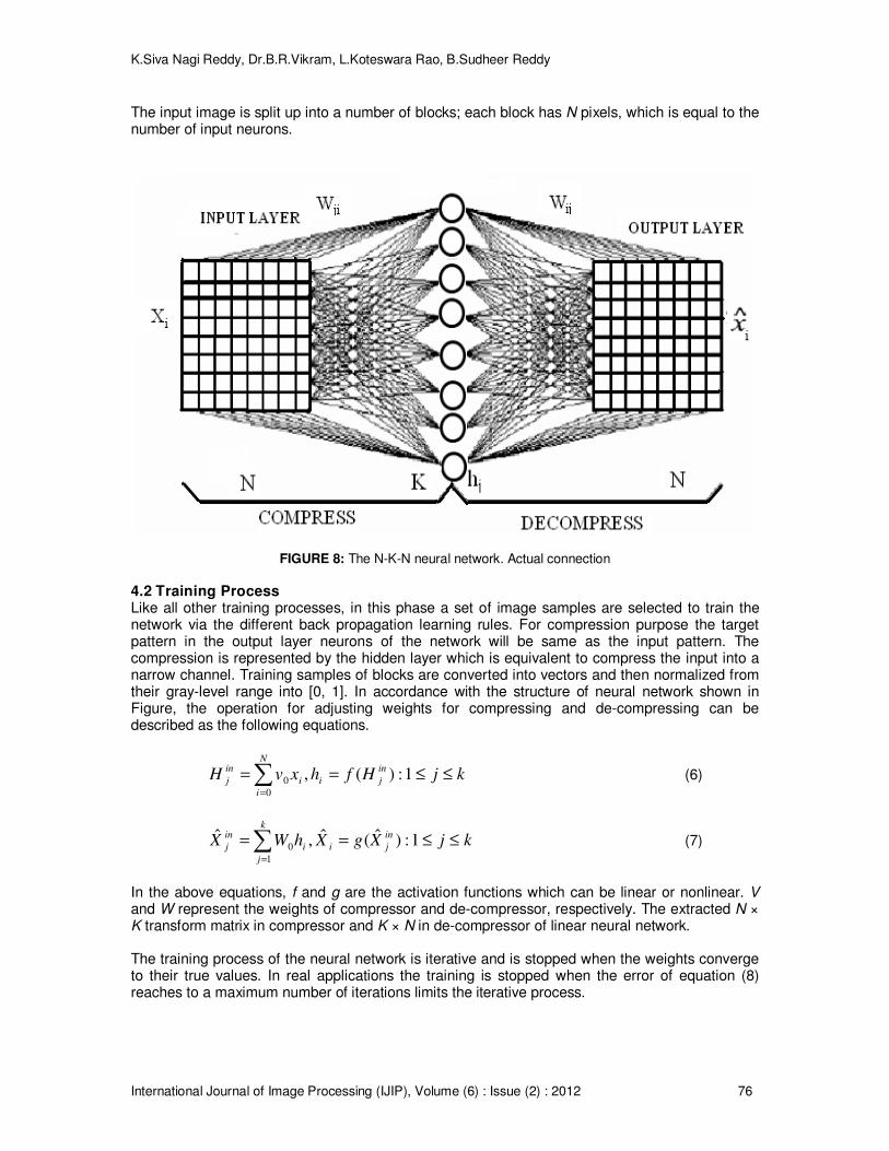
4. MULTI-LAYER NEURAL NETWORKS FOR IMAGE COMPRESSION Multi-Layer neural networks with back-propagation algorithm can directly be applied to image compression. The simplest neural network structure for this purpose is illustrated in Fig. 7. This network has three layers, input, hidden and output layer. Both the input and output layers are fully connected to the hidden layer and have the same number of neurons, N. Compression can be achieved by allowing the value of the number of neurons at the hidden layer, K, to be less than that of neurons at both input and output layers ( K ≤ N ). As in most compression methods, the input image is divided apart into blocks, for example with 8×8, 4× 4 or 16 ×16 pixels. These block sizes determine the number of neurons in the input/output layers which convert to a column vector and fed to the input layer of network; one neuron per pixel. With this basic MLP neural network, compression is conducted in training and application phases as follow.

FIGURE 7: Neural Network Structure

4.1 The Neural Network Architecture The Back propagation (BP) is one of neural networks, which are directly applied to image compression. The network structure is shown in Figure 8. This structure referred to feed forward auto associative type network. The input layer and output layer are fully connected to the hidden layer. Compression is achieved by estimating the value of K, the number of neurons at the hidden layer less than that of neurons at both input and the output layers. In the given Architecture “N” is number of neurons in input or output layer and the K is the number of neurons of hidden layer.



The input image is split up into a number of blocks; each block has N pixels, which is equal to the number of input neurons.

FIGURE 8: The N-K-N neural network. Actual connection

4.2 Training Process Like all other training processes, in this phase a set of image samples are selected to train the network via the different back propagation learning rules. For compression purpose the target pattern in the output layer neurons of the network will be same as the input pattern. The compression is represented by the hidden layer which is equivalent to compress the input into a narrow channel. Training samples of blocks are converted into vectors and then normalized from their gray-level range into [0, 1]. In accordance with the structure of neural network shown in Figure, the operation for adjusting weights for compressing and de-compressing can be described as the following equations.

kjHfhxvHin

ji

N

i

i

in

j ≤≤==∑=

1:)(,0

0 (6)

kjXgXhWX in

j

k

j

ii

in

j≤≤==∑

=

1:)ˆ(ˆ,ˆ

1

0 (7)

In the above equations, f and g are the activation functions which can be linear or nonlinear. V and W represent the weights of compressor and de-compressor, respectively. The extracted N × K transform matrix in compressor and K × N in de-compressor of linear neural network. The training process of the neural network is iterative and is stopped when the weights converge to their true values. In real applications the training is stopped when the error of equation (8) reaches to a maximum number of iterations limits the iterative process.



FIGURE 9: Architecture of Neural Network Structure at the time of Training

Preparation of NN Training/testing Set A testing set consists of sub images that are not included in the training set and it is used to assess the NN performance after training. The preparation of training/testing set includes the following steps: Step 1: Apply the segmentation process on the image to be used in learning/testing processes. Step 2: Apply rasterization and normalization on every block segment. Step 3: Store the results in the training set file. Step 4: Repeat from Step 1 while there are more images to be used in training process. 4.3 Learning Algorithms

4.3.1 Levenberg-Marquardt Algorithm (LM) For LM algorithm [16, 17], the performance index to be optimized is defined as

F (w) =∑ [∑ (dkp- okp) 2] (8)

Where w= [w1 w2 …. wN]

T consists of all weights of the network, dkp is the desired value of the k

th

output and the pth pattern, okp is the actual value of k

th output and the p

th pattern is the number of

the weights, P is the number of patterns, and K is the number of network outputs. Equation (8) can be written as

F (w) = ET E (9)

In above equation E is the Cumulative Error Vector (for all patterns)

E= [e11… ek1 e12... ek2 … ekp]T ekp= dkp- okp, k=1...K, p=1.…P

From equation (9) the Jacobin matrix is defined as



J (w) =

∂

∂

∂

∂

∂

∂

∂

∂

∂

∂

∂

∂∂

∂

∂

∂

∂

∂

∂

∂

∂

∂

∂

∂

∂

∂

∂

∂

∂

∂∂

∂

∂

∂

∂

∂

N

kpkpkp

N

ppp

N

ppp

N

kkk

N

N

w

e

w

e

w

e

w

e

w

e

w

e

w

e

w

e

w

e

w

e

w

e

w

e

w

e

w

e

w

e

w

e

w

e

w

e

L

MLMM

L

L

MLMM

L

MMMM

L

L

21

2

2

2

1

2

1

2

1

1

1

1

2

1

1

1

21

2

21

1

21

11

2

11

1

11

(10)

And the weights are calculated using the following equation using Newton method

)())()(1

1

k

T

ttktk

T

tk

wjIwJwJk ww

−+−+ = α (11)

Where “I” is identity unit matrix, “α” is a learning factor and “J” is Jacobin of m output errors with respect to n weights of the neural network. For α=0 it becomes the Gauss-Newton method. If “α” is very large The LM algorithm becomes the steepest decent or the EBP algorithm. The “α” parameter is automatically adjusted for all iterations in order to secure convergence. The LM algorithm requires computing of the Jacobin J Matrix at each iteration step and the inversion of J

TJ square matrix. Note that in the LM algorithm an N by N matrix must be inverted for all

iterations. This is the reason why for large size neural networks the LM algorithm is not practical. We are proposing another method that provides a similar performance, while lacks the inconveniences of LM, and is more stable. 4.3.2 Modification of the LM Algorithm Instead of the performance index given by (8), the following new performing index is introduced

2

1

2

1

])([)( ∑ ∑= =

−=k

k

p

p

kpkp odwF (12)

This form of the index, which represents a global error, will later lead to a significant reduction of the size of a matrix to be inverted at each iteration step. Equation (12) can be also written as:

EEwFT ∧

=)( (13)

Where E = [ 1e , 2e ,…. Ke ]T

, Ke ==∑=

−P

P

kpkp od1

2 ])( At k=1……k

Now the modified Jacobin matrix can be defined as



∂

∂

∂

∂

∂

∂

∂

∂

∂

∂

∂

∂∂

∂

∂

∂

∂

∂

=

N

kkk

N

N

w

e

w

e

w

e

w

e

w

e

w

e

w

e

w

e

w

e

wj

)

L

))MLMM

)

L

))

)

L

))

21

1

2

2

1

2

1

2

1

1

1

)(ˆ (14)

And the equation (11) can be written using modified Jacobin matrix

wk+1= wk-(T

tJ ( )kw1

))(ˆ −+ IwJ tkt α T

tJ ( )kw tE (15)

Note is a K by N matrix, and it leads to inverting an N by N matrix. Here N is the number of weights. This problem can be further simplified using the matrix Inversion. This states that if a matrix O satisfies

O=P-1

+QR-1

RT (16)

O-1

=P-PQ(R+QTPQ)

-1Q

TP (17)

O = tJ ( )kwT

tJ ( )kw + Itα (18)

P= Itα

1 (19)

Q = T

tJ ( )kw (20)

R=I (21)

By Substituting equations (18), (19), (20) and (21) into equation (17), that can obtain

(T

tJ ( )kw )(ˆkt wJ +I)

1−= I

tα

1-

2

1

tαT

tJ ( )kw (1+

tα

1)(ˆ

kt wJT

tJ ( )kw )-1 )(ˆ

kt wJ (22)

Note that in the right side of equation (22), the matrix to be inverted is of size K by K. In every application, N, which is the number of weights, is much greater than K, which is number of outputs. By inserting equation (22) into equation (15) one may have

Ik

tk

ww α

11

−+ = -2

1

tαT

tJ ( )kw (1+

tα

1)(ˆ

kt wJT

tJ ( )kw )-1 )(ˆ

kt wJ ] (T

tJ ( )kw tE (23)

For single output networks, equation (17) becomes

∧∧

+

<−−=+ EwJww

tk

T

tk

T

tktt

k

T

tkt

i

kkwJwJ

JwJI )(]

)(ˆ)(ˆ

)(ˆ)(ˆ[

11 αα

(24)

As known learning factor, “α” is illustrator of actual output movement to desired output. In the standard LM Method”α” is a constant number. In this method “α” is been modified as “0.01 E

TE”,

Where E is a k x 1 matrix therefore ETE is a 1 x 1 therefore [J

TJ + αI] is invertible. From the

equation (24) matrix inversion is not required at all. Therefore if actual output is far than desired output or similarly, errors are large so it converges to desired output with large steps. Likewise when measurement of error is small then actual output approaches to desired output.



NN learning Algorithm Steps Step 1: Initialization of network weights, learning rate and Threshold error. Set iterations to zero. Step 2: Total error = zero; iterations → iterations+1. Step 3: Feed one vector to the input layer. Step 4: Initialize the target output of that vector. Step 5: Calculate the outputs of hidden layer units. Step 6: Calculate the outputs of output layer units. Step 7: Calculate error (desired output - actual output) and calculate total error. Step 8: Calculate New Error of output layer units and adjust weights between output and hidden layer. Step 9: Calculate New Error of hidden layer units and adjust weights between hidden and input layer. Step 10: While there are more vectors, go to Step 3. Step 11: If Threshold error >= Total error then stop, otherwise go to Step 2.

5. NN COMPRESSION PROCESS The compression process Step 1: Read image pixels and then normalize it by converting it from range [0-255] to range [0-1]. Step 2: Divide the image into non-overlapping blocks. Step 3: Rasterizing the image blocks. Step 4: Apply the rasterized vector into input layer units Step 5: Compute the outputs of hidden layer units by multiplying the input vector by the weight matrix (V). Step 6: Store the outputs of hidden layer units after renormalizing them in a compressed file. Step 7: If there are more image vectors go to Step 4.

FIGURE10: Neural Network Structure Compression

Decompression Process Step 1: Take one by one vector from the compressed image. Step 2: Normalize this vector (it represents the outputs of hidden layer units). Step 3: The outputs of output layer units by multiplying outputs of hidden layer units by the weight matrix



Step 4: Derasterize the outputs of output layer units to build the sub image Step 5: Return this sub image to its proper location Step 6: Renormalize this block and store it in the reconstructed file. Step 7: If there are more vectors go to Step 1.

FIGURE 11: Neural Network Structure Decompressions

6. EXPERIMENT RESULTS The quality of an image is measured using the parameters like Mean Square Error (MSE) and Peak Signal to Noise ratio (PSNR). MSE and PSNR are the parameters which define the quality of an image reconstructed at the output layer of neural network. The MSE between the target image and reconstructed image should be as small as possible so that the quality of reconstructed image should be near to the target image. Ideally, the mean square error should be zero for ideal decompression. The compression-decompression error is evaluated by comparing the input image and decompressed image using normalized mean square error formulas. In ANN image compression system, the CR is defined by the ratio of the data fed to the input layer Neurons (Ni) to the data out from the hidden layer neurons (Nh). Also the Compression Ratio Performance can be computed by the equation:

%100))/1( XNNCR ih−= (25)

Transmission Time is the ratio of number of pixel × number of bits pixel / Modem Speed (Kilo bytes/sec). The MSE metric is most widely used for it is simple to calculate, having clear physical interpretation and mathematically convenient. MSE is computed by averaging the squared intensity difference of reconstructed image ŷ and the original image, y. Then from it the PSNR is calculated. Mathematically,

2][

1

yyk

kCDMSE

∧−= (26)



In this section, the implementation results of the compression algorithms with structure are studied and compared with Levenberg-Marquardt Algorithm and Modified Levenberg-Marquardt Algorithm Evaluation criteria used for comparison, is compression ratio and the PSNR. For an Image with C rows and D columns PSNR is defined as follow:

)](/255[10 2

10log dbMSEPSNR = (27)

Where C is Row D is Column .In above equation 255 represents maximum gray level value in an 8-bit image. This criterion is an acceptable measurement for assessing the quality of the reconstructed image. In both structures image blocks of size 8×8 were used and as a result both input and output layer have 64 neurons. In a structure 1, 016 neurons were used in the hidden layer .so it will results in the fixed 4:1 compression ratio. This structure was trained with the 64× 64,128×128,256×256 with standard Image which Includes 1024 training pattern. The experimental results are shown in Table1, 2and 3. One can easily conclude that this structure has a favorable result on the trained Images.

64 x 64 Modified Levenberg-Marquardt

Algorithm Levenberg-Marquardt Algorithm

Images PSNR MSE TIME PSNR MSE TIME

Lena 32.749 13.8412 312.69 31.1650 14.2209 950.047

Crowd 18.8411 33.9374 297.61 16.369 35.1832 908.957

Pepper 26.9293 17.4648 323.91 23.5447 18.5536 1006.22

Cameraman 22.2501 58.4495 303.02 20.2811 62.6332 876.423

TABLE 1: Performance and comparison of existing and proposed technique for image size 64 X 64

128 x128 Modified Levenberg-Marquardt



Lena 35.3545 20.6128 1270.701 33.9659 20.2829 3869.427

Crowd 22.4568 33.5796 3515.639 18.6568 35.2746 3635.639

Pepper 28.3607 28.2945 3683.412 27.2607 20.3975 3883.412

Cameraman 29.1466 16.5404 3542.444 28.2466 18.0402 3742.444




256 x256 Modified Levenberg-Marquardt



Lena 38.6035 20.1279 3270.10

1 36.6596 21.1839 3669.274

Crowd 23.4564 30.2496 3115.33

9 21.5686 35.1796 3515.396

Pepper 32.1603 24.2945 3983.11

2 28.6076 30.3454 3783.124

Cameraman 34.5466 28.3043 4042.26

4 30.4662 30.104 3342.444




FIGURE 12: Neural Network compressions FIGURE 13: Neural Network Reconstruction

7. CONCLUSION In this paper the use of Multi -Layer Perception Neural Networks for image compression is reviewed. Since acceptable result is not resulted by compression with one network, a new approach is used by changing the Training algorithm of the network with modified LM Method. The proposed technique is used for image compression. The algorithm is tested on varieties of benchmark images. Simulation results for standard test images with different sizes are presented. These results are compared with L-M method. Several performance measures are used to test the reconstructed image quality. According to the experimental results, the proposed technique with modified L-M method outperformed the existing method. It can be inferred from experimental results as shown in Table 1, 2 and 3 that the proposed method performed well and results higher compression ratio. Besides higher compression ratio it also preserves the quality of the image. It can be concluded that the integration of classical with soft computing based image compression enables a new way for achieving higher compression ratio.

REFERENCES [1] R. P. Lippmann, “An introduction to computing with neural network”, IEEE ASSP mag., pp. 36-54,

1987. [2] M.M. Polycarpou, P. A. Ioannou, “Learning and Convergence Analysis of Neural Type Structured

Networks”, IEEE Transactions on Neural Network, Vol 2, Jan 1992, pp.39-50. [3] K. R Rao, P. Yip, Discrete Cosine Transform Algorithms, Advantages, Applications, Academic Press,

1990 [4] Rao, P.V. Madhusudana, S.Nachiketh,S.S.Keerthi, K. “image compression using artificial neural

network”.EEE, ICMLC 2010, PP: 121-124. [5] Dutta, D.P.; Choudhury, S.D.; Hussain, M.A.; Majumder, S.; ”Digital image compression using

neural network” .IEEE, international Conference on Advances in Computing, Control, Telecommunication Technologies, 2009. ACT '09.

[6] N.M.Rahim, T.Yahagi, “Image Compression by new sub-image bloc Classification techniques using

Neural Networks”, IEICE Trans. On Fundamentals, Vol. E83-A, No.10, pp 2040-2043, 2000. [7] M. S. Rahim, "Image compression by new sub- image block Classification techniques using

neural network. IEICE Trans. On Fundamentals of Electronics, Communications, and Computer Sciences, E83-A (10), (2000), pp. 2040- 2043.



[8] D. Anthony, E. Hines, D. Taylor and J. Barham, “A study of data compression using neural networks

and principal component analysis, “in Colloquium on Biomedical Applications of Digital Signal Processing,1989, pp. 1–5.

[9] G. L. Sicuranzi, G. Ramponi, and S. Marsi, “Artificial neural network for image compression,”

Electronics Letters, vol. 26, no. 7, pp. 477– 479, March 29 1990. [10] M.Egmont-Petersen, D.de.Ridder, Handels, “Image Processing with Neural Networks – a review”,

Pattern Recognition 35(2002) 2279-2301 [11] M. H. Hassoun, Fundamentals of Artificial Neural Networks, MIT Press, Cambridge, MA, 1995.

[12] Wasserman, P.D., 1989. Neural Computing: Theory and Practice. Coriolis Group, New York, USA,

ISBN: 10: 0442207433, pp: 230. [13] Durai S.A. And E.A. Saro, 2006. Image compression with back-propagation neural network using

cumulative distribution function. World Acad. Sci. Eng. Technol., 17: 60-64. [14] Xianghong, T. And L. Yang, 2008. An image compressing algorithm based on classified blocks

with BP neural networks. Proceeding of the International Conference on Computer Science and Software Engineering, Dec. 12-14, IEEE Computer Society, and Wuhan, Hubei pp: 819-822.

[15] Veisi, H. And M. Jamzad, 2009. A complexity-based approach in image compression using neural

networks. Int. J. Sign. Process. 5: 82-92. [16] B. M. Wilamowski, Y. Chen, A. Malinowski, “Efficient algorithm for training neural networks with one

hidden layer,” In Proc. IJCNN, vol.3, pp.1725-728, 1999. [17] T. Cong Chen, D. Jian Han, F. T. K. Au, L. G.Than, “Acceleration of Levenberg-Marquardt training of

neural networks with variable decay rate”, IEEE Trans. on Neural Net., vol. 3, no. 6, pp. 1873 - 1878, 2003. World Academy of Science, Engineering and Technology 6 2005.

Image Processing Compression and Reconstruction by Using New Approach Artificial Neural Network

Education

Transcript of Image Processing Compression and Reconstruction by Using New Approach Artificial Neural Network