![A Simple Model for Intrinsic Image Decomposition with ...vladlen.info/papers/intrinsic-RGBD.pdfviewpoint [34, 24, 23], using manual annotation to guide thedecomposition[10,27], andusingcollectionsofimages](https://static.fdocuments.in/doc/165x107/5f9d249d5c536c27d32c3479/a-simple-model-for-intrinsic-image-decomposition-with-viewpoint-34-24-23.jpg)
Image Holistic Scene Understanding Based on Image Intrinsic ...
20
International Journal of Signal Processing, Image Processing and Pattern Recognition Vol.9, No.3 (2016), pp.17-36 http://dx.doi.org/10.14257/ijsip.2016.9.3.03 ISSN: 2005-4254 IJSIP Copyright ⓒ 2016 SERSC Image Holistic Scene Understanding Based on Image Intrinsic Characteristics and Conditional Random Fields Lin Li Institute of Intelligent Computing and Information Technology, Chengdu Normal University, Chengdu, 611130, China [email protected] Abstract Image holistic scene understanding based on image intrinsic characteristics and conditional random fields is proposed. The model integrates image scene classification, image semantic segmentation and object detection. 1) For the scene classification, we use method of PHOW feature extraction plus KPCA dimensional reduction to obtain feature information for each image. 2) For object detection section, saliency detection and segmentation characteristics of the image object detection is useful. We propose the method by integrating image segmentation information got by the method proposed in literature [1]. 3) For the semantic segmentation: (1) For the unary potentials, we incorporating HOG, RGB color histogram and LBP features by the methods proposed in literature [2]; (2) The image manifold structural features can better reflect the importance between hyper-pixel regions and eventually boost accuracy. Therefore, we add the higher-order potential item to reflect inherent manifold image feature of each super pixel region. The experiments testify that model performance has raised on all three sub-tasks. Keywords: image holistic scene understanding, scene understanding, conditional random fields, image intrinsic characteristics, probabilistic graphical model 1. Introduction One main purpose of computer vision is to let the computer understand the real world by the digital signal processing, this is the so-called visual perception. However, there is an ill-posed problem that the solution is not unique for a lot of problems, and continuous dependent on the initial data[3]. The undirected graph model has its unique advantages to reveal spatial dependence relationship of a real scene in the field of image understanding. It has a wide range of applications such as image annotation, segmentation, de-noising, etc.[4]. The typical representatives of the undirected graph are MRF (Markov Random Fields) and CRF (Conditional Random Fields) models. The image understanding based on the undirected graph model can be formulated by a mathematical description[5]. The assumption that D represents the observing data, x is the problem solution vector for related visual perception, so the problem of visual perception can be seen as the mapping from D to x that is an inverse problem solved by optimization, as shown in equation(1). arg min (, | ) opt x E x xDw (1) Where, w is the model parameter, (, , ) E xDw is the potential function (so called cost or object function) that is a quality measure function in solution space with the observing data D , and parameter configuration w and x . Thus, visual problems are related to modeling (establishing suitable potential energy function), parameter learning (finding the
Transcript of Image Holistic Scene Understanding Based on Image Intrinsic ...

International Journal of Signal Processing, Image Processing and Pattern Recognition
Vol.9, No.3 (2016), pp.17-36
http://dx.doi.org/10.14257/ijsip.2016.9.3.03
ISSN: 2005-4254 IJSIP
Copyright ⓒ 2016 SERSC
Image Holistic Scene Understanding Based on Image Intrinsic
Characteristics and Conditional Random Fields
Lin Li
Institute of Intelligent Computing and Information Technology, Chengdu Normal
University, Chengdu, 611130, China
Abstract
Image holistic scene understanding based on image intrinsic characteristics and
conditional random fields is proposed. The model integrates image scene classification,
image semantic segmentation and object detection. 1) For the scene classification, we use
method of PHOW feature extraction plus KPCA dimensional reduction to obtain feature
information for each image. 2) For object detection section, saliency detection and
segmentation characteristics of the image object detection is useful. We propose the
method by integrating image segmentation information got by the method proposed in
literature [1]. 3) For the semantic segmentation: (1) For the unary potentials, we
incorporating HOG, RGB color histogram and LBP features by the methods proposed in
literature [2]; (2) The image manifold structural features can better reflect the
importance between hyper-pixel regions and eventually boost accuracy. Therefore, we
add the higher-order potential item to reflect inherent manifold image feature of each
super pixel region. The experiments testify that model performance has raised on all three
sub-tasks.
Keywords: image holistic scene understanding, scene understanding, conditional
random fields, image intrinsic characteristics, probabilistic graphical model
1. Introduction
One main purpose of computer vision is to let the computer understand the real world
by the digital signal processing, this is the so-called visual perception. However, there is
an ill-posed problem that the solution is not unique for a lot of problems, and continuous
dependent on the initial data[3]. The undirected graph model has its unique advantages to
reveal spatial dependence relationship of a real scene in the field of image understanding.
It has a wide range of applications such as image annotation, segmentation, de-noising,
etc.[4]. The typical representatives of the undirected graph are MRF (Markov Random
Fields) and CRF (Conditional Random Fields) models.
The image understanding based on the undirected graph model can be formulated by a
mathematical description[5]. The assumption that D represents the observing data, x is
the problem solution vector for related visual perception, so the problem of visual
perception can be seen as the mapping from D to x that is an inverse problem solved by
optimization, as shown in equation(1).
argmin ( , | )opt
xEx x D w (1)
Where, w is the model parameter, ( , , )E x D w is the potential function (so called cost
or object function) that is a quality measure function in solution space with the observing
data D , and parameter configuration w and x . Thus, visual problems are related to
modeling (establishing suitable potential energy function), parameter learning (finding the
International Journal of Signal Processing, Image Processing and Pattern Recognition
Vol.9, No.3 (2016)
18 Copyright ⓒ 2016 SERSC
optimal configuration through the training data) and model reasoning (solving
optimization optx ).
The undirected graph model has obvious advantages[5]: 1) MRF provides a modular,
flexible and principled approach which can integrates the normalized data (with a prior
information), the data likelihood and other useful clues including continuous and discrete
information in the graphical models; 2) Graph theory provides a simple visual model
structure easy for model parameter selection and design; 3)The reasoning problem of joint
probability graph model is solved by graph factorization, especially based on discrete
optimization inference, enhanced discrete MRF potential, significantly expanded the
scope of application of the perception problem; 4) Finally, from a probability perspective
MRF has great advantages of parameter learning, the classical variation method for
uncertainties problems.
Currently, the undirected graph model in computer vision and image understanding is
very common. There is a lot of very successful model [6-12], and some based on the
holistic scene understanding CRF model also achieving notable success[13, 14]. However,
there is still many problems need to be solved in the image understanding system based
on the undirected graph model.
First, from the modeling perspective, in theory, a lot of image understanding and
inverse problems are ill-posed problem, which requires a lot of observed variables implied
to express expectation change of perceptual problem. In addition, observations are usually
noisy, imperfect, and may provide only partial information. Therefore, the model needs to
have a good regularization, robust data metrics and compact structure variables to reflect
the relationship between them, and this relationship is often unknown. So there are a lot of
problems needed to be addressed and solved.
Second, the complexity of the model reasoning traceability, the optimization quality
and etc. also need further study.
Third, the feature representation of undirected graph has many research content, there
are currently no universally accepted theory and architecture system.
Finally, the image holistic scene understanding based on undirected graph is still in the
inception stage, there are many shortcomings that need further research.
2. Related Works
The key motivation behind the holistic scene understanding, tracing back to the
seminal work of Barrow in the 70s [15], is that ambiguities in visual information can only
be resolved when many visual processes are working collaboratively. There are few
efforts on the joint reasoning of the various recognition tasks. Combining contextual
scene information, object detection and segmentation has also been tackled in the past.
The contextual information is incorporated into a CRF leading to improved object
detection by Torralba [16]. Spatial contextual interactions between objects have also been
modeled[17, 18]. Joint estimation of depth, scene type, and object locations is performed
in [19]. Image segmentation and object detection are jointly modeled in [7, 20].
A more holistic approach to combine detection and segmentation is proposed in [21],
defining the joint inference within a CRF framework. However, their joint inference does
not improve performance significantly and/or rely on complex merging/splitting moves.
The literature [10] is the most comprehensive understanding of the holistic scene model
based on the CRF, simultaneously achieving three tasks of object detection, classification
and semantic scene segmentation. However, its own shortcomings affect the performance:
1) the representation of unit potential and classification feature of the model is not fully
explored; 2) The image super-pixel local features also need further research such as image
intrinsic manifold structure.
Inspired by [15], In this study, we explore the intrinsic characteristics of the image, in
order to improve and enhance the holistic image scene understanding.

International Journal of Signal Processing, Image Processing and Pattern Recognition
Vol.9, No.3 (2016)
Copyright ⓒ 2016 SERSC 19
3. Our Holistic Scene Understanding Framework
We present a new framework for image holistic understanding of the image holistic
scene understanding and exploration of image intrinsic characteristics in this section: first,
we build a whole scene understanding CRF model, which defines a unified semantic CRF
integrating three sub-tasks of semantic segmentation, object detection and scene
classification.
As shown in Figure 1, the random field contains variables representing the class labels
of image segments at two levels in a segmentation hierarchy (segments and larger super-
segments) as well as binary variables indicating the correctness of candidate object
detections.
Let 1,...,ix C be a random variable representing the class label of the i-th segment in
the lower level of the hierarchy. 1,...,jy C is a random variable associated with the
class label of the j-th segment of the second level of the hierarchy. 0,1lb is be a binary
random variable associated with a candidate detection, taking value 0 when the detection
is a false detection.
We define the holistic understanding of the CRF model as follows:
1
( , , , , ) type
type
p
x y z b s AZ
(2)
Here, type
encodes potential functions over sets of variables. For clarity, we describe
the potentials in the log domain, i.e., logtype
typew . We employ a different weight
for each type of potential, and share the weights across cliques. We learn the weights from
training data using the structure prediction framework of literature [22] by defining
appropriate loss functions for the holistic task.
Scene
Class
Object
class
Object
detecion
PHOW+KPCA feature
Saliency segmentation
Superpexel
segmentation
Building
Grass
Sign
Biycle
Aeroplane
Road
Mountains
Car
Chair
Body
Cow
Car
Aeroplane
Face
Tree
Bird
Chair
Grass
Boat
Book
Image
Image intrinsic manifold
(a)
(c)
(d)
100 200 300 400 500 600 700 800
200
400
600
HOG feature
Color histogram feature
0 10 20 30 40 50 600
2
4
6x 10
4 LBP feature
(e)
(b)
(f)
ix
jy
lb
s
kz On
Off
Figure 1. The Holistic Scene Understanding Framework
International Journal of Signal Processing, Image Processing and Pattern Recognition
Vol.9, No.3 (2016)
20 Copyright ⓒ 2016 SERSC
The main difference between the our proposed holistic scene understanding based on
CRFs with literature [10] is that, according to the image intrinsic characteristics, the
model incorporates three aspects of information as follows:
1) For scene classification section: We incorporate the overall image feature
information by using the method of literature [23] PHOW plus KPCA dimensionality
reduction to obtain each image feature information, as shown in Figure 1 (a).
2) For the object detecting section: saliency detection and segmentation characteristic
has important roles in the object detection. We use the method of literature [1] in order to
find more accurate object position, shown in Figure 1 (b).
3) For the semantic segmentation parts: (1) we improve unary potential representation
by incorporating HOG features, RGB color histogram features and LBP features, with
similar way as literature [2] to get unary potential based on super-pixel region, as shown
in Figure 1 (c-e). (2) We believe that the inherent manifold features within an image can
better reflect the importance of superpixel areas that will improve the final segmentation
accuracy. Thus we add higher-order potential items for the inherent manifold feature of
each super-pixel area within the image, as shown in Figure 1 (f).
It must be said that Figure 1 doesn't show all of the information, we only render our
added or emphasized feature information for improving the three sub-tasks.
4. Image Intrinsic Feature Fusion
4.1. Unary Potential Feature Information
As the unary potential for semantic segmentation, the features we incorporated are as
follows:
1) Image texton features have been proven effective in the general classification and
object detection. The texton dictionary is obtained by the K-means clustering with 17-
dimensional filter banks on training samples. Each pixel in the image is assigned to its
nearest cluster center, eventually forming texton map.
2) Shape filter is composed by a set of rectangular regions RN , which are the four
corners of the image in more than half of the area of a bounding box arbitrarily selected.
For a particular texton t, the feature response at the location i is the count of instances of
that texton under the offset rectangle mask.
3) HOG feature information: The core idea of HOG is that local object shape can be
detected or described by the distribution of light intensity gradient or edge direction. The
feature reflects the inherent characteristics of the image, which has a positive effect on
image segmentation, as shown in Figure 1 (c).
4) RGB histogram feature information is got by separating the color image into three
channels, as shown in Figure 1 (d).
5) LBP feature information is an effective texture feature representation which has the
characterization of robust illumination, rotation invariation as shown in Figure 1 (e).
The unary potential feature information is acquired through learning a multi-class
classifier by using an adapted version of the joint boosting algorithm of literature[24].
The algorithm iteratively builds a strong classifier as a sum of ‘weak classifiers’,
simultaneously selecting discriminative features. Each weak classifier is a decision stump
based on a threshold feature response, and is shared among a set of classes, allowing a
single feature to help classify several classes at once.
International Journal of Signal Processing, Image Processing and Pattern Recognition
Vol.9, No.3 (2016)
Copyright ⓒ 2016 SERSC 21
4.2. Image Manifold Feature Information
Image manifold feature information is very important in exploring the intrinsic
characteristics within the image. In this study, we add superpixel potential based on
manifold ranking for semantic segmentation.
The graph-based ranking problem is described as follows: given a node as a query, the
remaining nodes are ranked based on their relevance to the given query. The goal is to
learn a ranking function, which defines the relevance between unlabeled nodes and
queries.
4.2.1. Manifold Ranking: Given a dataset 1 1,..., , ,..., n
l l nx x x x X R some data points
are labelled queries and the rest need to be ranked according to their relevance to the
queries. Let : nf X R denote a ranking function which assigns a ranking value if to
each point ix . f can be viewed as a vector 1,...,T
nf ff . Let 1 2, ,...,T
ny y yy denote
an indication vector, in which 1iy , if ix is a query, and 0iy otherwise. Let
,G V E denote a graph on dataset, where notes v are the dataset, and the edges E are
weighted by an affinity matrix ij n nw
w . The degree matrix is 11,..., nndiag d dD
where ii ijjd w . Similar to the PageRank
[25], the optimal ranking of queries is
computed by solving the following optimization problem:
2, 1 1
2
1* argmin
2
n nji
ij i if i j iii jj
fff w f y
d d
(3)
Where the parameter controls the balance of the smoothness constraint (the first
term) and the fitting constraint (the second term). The minimum solution is computed by
setting the derivative of the above function to be zero. The resulted ranking function can
be written as:
1
*
f D W y (4)
where I is an identity matrix, 1/ 1 and S is the normalized Laplacian matrix,
1/2 1/2/ s d wd .
4.2.2. Superpixel segmentation: In this study, we use the UCM (Ultrametric Contour
Map) [26]
for superpixel segmentation.
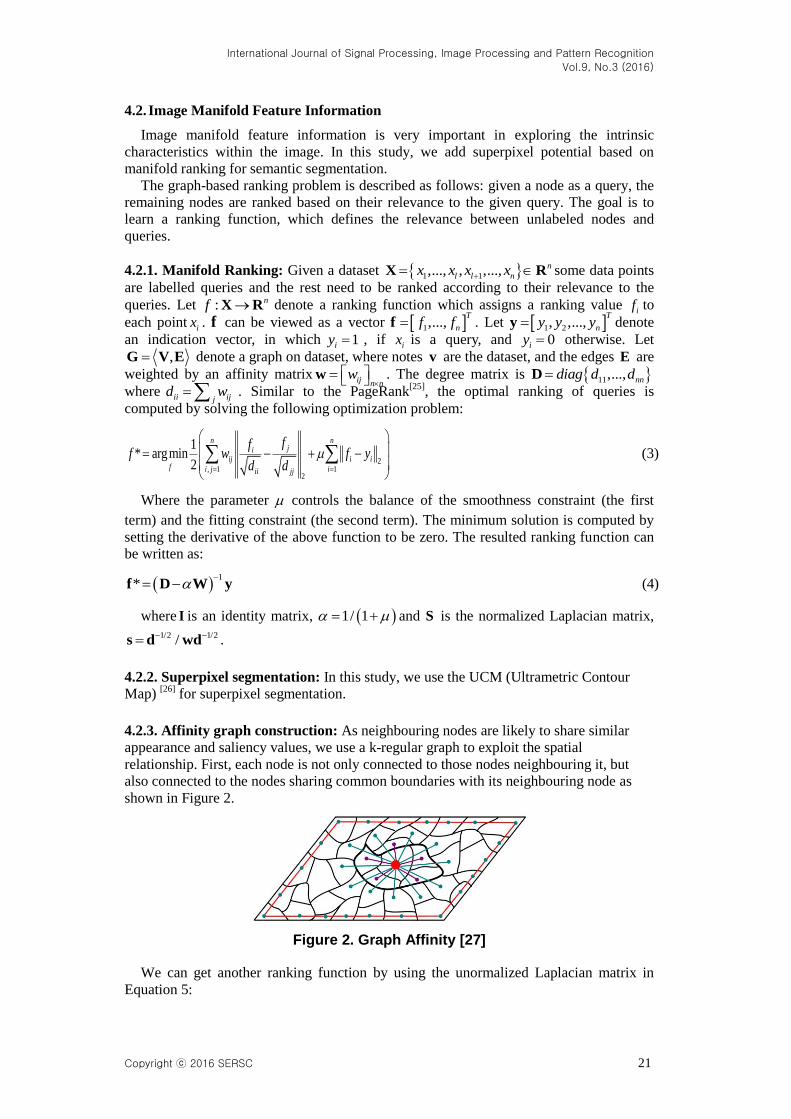
4.2.3. Affinity graph construction: As neighbouring nodes are likely to share similar
appearance and saliency values, we use a k-regular graph to exploit the spatial
relationship. First, each node is not only connected to those nodes neighbouring it, but
also connected to the nodes sharing common boundaries with its neighbouring node as
shown in Figure 2.
Figure 2. Graph Affinity [27]
We can get another ranking function by using the unormalized Laplacian matrix in
Equation 5:
International Journal of Signal Processing, Image Processing and Pattern Recognition
Vol.9, No.3 (2016)
22 Copyright ⓒ 2016 SERSC
2,
i j
ij
c cw e i j
V (5)
Where ic and jc denote the mean of the superpixels corresponding to two nodes in the
CIE LAB color space, and is a constant that controls the strength of the weight.
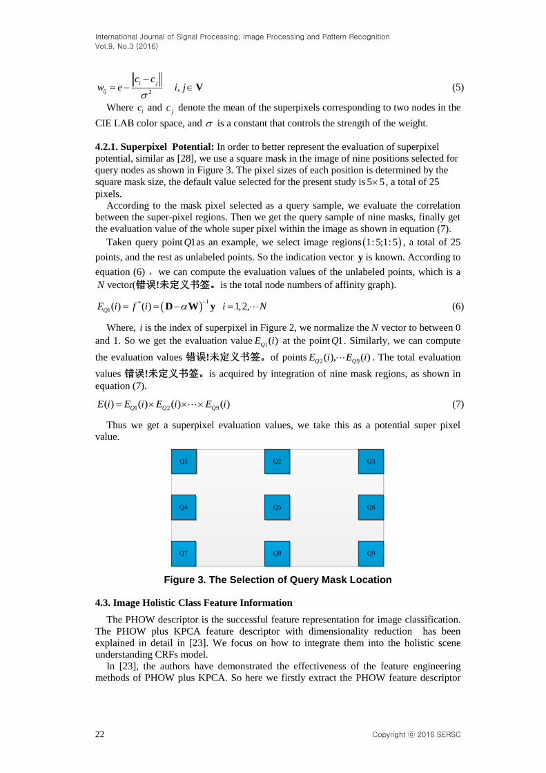
4.2.1. Superpixel Potential: In order to better represent the evaluation of superpixel
potential, similar as [28], we use a square mask in the image of nine positions selected for
query nodes as shown in Figure 3. The pixel sizes of each position is determined by the
square mask size, the default value selected for the present study is 5 5 , a total of 25
pixels.
According to the mask pixel selected as a query sample, we evaluate the correlation
between the super-pixel regions. Then we get the query sample of nine masks, finally get
the evaluation value of the whole super pixel within the image as shown in equation (7).
Taken query point 1Q as an example, we select image regions 1:5;1:5 , a total of 25
points, and the rest as unlabeled points. So the indication vector y is known. According to
equation (6) ,we can compute the evaluation values of the unlabeled points, which is a
N vector(错误!未定义书签。is the total node numbers of affinity graph).
1*
1( ) ( ) 1,2,QE i f i i N
D W y (6)
Where, i is the index of superpixel in Figure 2, we normalize the N vector to between 0
and 1. So we get the evaluation value 1( )QE i at the point 1Q . Similarly, we can compute
the evaluation values 错误!未定义书签。of points 2 9( ), ( )Q QE i E i . The total evaluation
values 错误!未定义书签。is acquired by integration of nine mask regions, as shown in
equation (7).
1 2 9( ) ( ) ( ) ( )Q Q QE i E i E i E i (7)
Thus we get a superpixel evaluation values, we take this as a potential super pixel
value.
Q1 Q2 Q3
Q4 Q5 Q6
Q7 Q8 Q9
Figure 3. The Selection of Query Mask Location
4.3. Image Holistic Class Feature Information
The PHOW descriptor is the successful feature representation for image classification.
The PHOW plus KPCA feature descriptor with dimensionality reduction has been
explained in detail in [23]. We focus on how to integrate them into the holistic scene
understanding CRFs model.
In [23], the authors have demonstrated the effectiveness of the feature engineering
methods of PHOW plus KPCA. So here we firstly extract the PHOW feature descriptor

International Journal of Signal Processing, Image Processing and Pattern Recognition
Vol.9, No.3 (2016)
Copyright ⓒ 2016 SERSC 23
plus KPCA dimensionality reduction of each image. Secondly, we train the SVM
classifier with hyper-parameter optimization and random kernel function selection.
Finally, the assessed value of each scene node is got by SVM classifier.
4.3. Image Saliency Detection Information
The bounding box detected by the model DPM (Deformed Part Model) [29]
, will always
exist non-object pixels. If the bounding box is directly used in the overall model to define
the potential entry, this will affect the final results of object detection.
We use the DPM method in the literature [29] to erase the interference of no-object
within bounding box.
(a)
(b)
Figure 4. The Schematic Diagram of Image Saliency Segmentation on Msrc-v2 Dataset
We use the method of direct saliency detection and segmentation proposed by Li et. al., [1]
as shown in Figure 4. The extraction object area is very accurate. However, the saliency
segmentation method does not accurately extract each object in region detection box, and
sometimes only a partial object segmentation, especially with DPM erroneous detection,
saliency segmentation method to extract the wrong area, this impacts the final
segmentation result. In experiments we find that the saliency segmentation region is often
only a small proportion of the rectangular bounding box area when this happens.
Therefore, similar to literature [1], when an area of saliency segmentation method is less
than 50% of the area of the bounding box, then ignore the detection bounding box. We
enhance the accuracy of the detection bounding box by this method. We select the largest
bounding box generated from the DPM candidate border, and then extract the real target
area, thus avoid interference of non-target pixel information for final object detection. We
define object detecting potential by using the detected saliency area, add a factor in
detecting potential. The factor is the boundary box saliency proportion of the entire
area of the object for reflecting the correlation of the object detection, the greater factor ,
and the higher is the correlation of detection.
5. Feature Engineering of Holistic Scene Understanding
Now, we describe the feature engineering. The segmentation potential, class presence
potential and scene potential are similar to literature [10]. The main difference is
manifested in higher order potential.
5.1. Segmentation Potential
5.1.1. Unary Segmentation Potential: We compute the unary potential for each region at
segment and super-segment level by averaging the TextonBoost[2]
pixel potentials inside
each region. This is done by training by TextonBoost method with texture feature, shape
filter, HOG, LBP and RGB. So, the segmentation potential ( | )s ix I and ( | )s jy I are
only dependent on Image I itself.
International Journal of Signal Processing, Image Processing and Pattern Recognition
Vol.9, No.3 (2016)
24 Copyright ⓒ 2016 SERSC
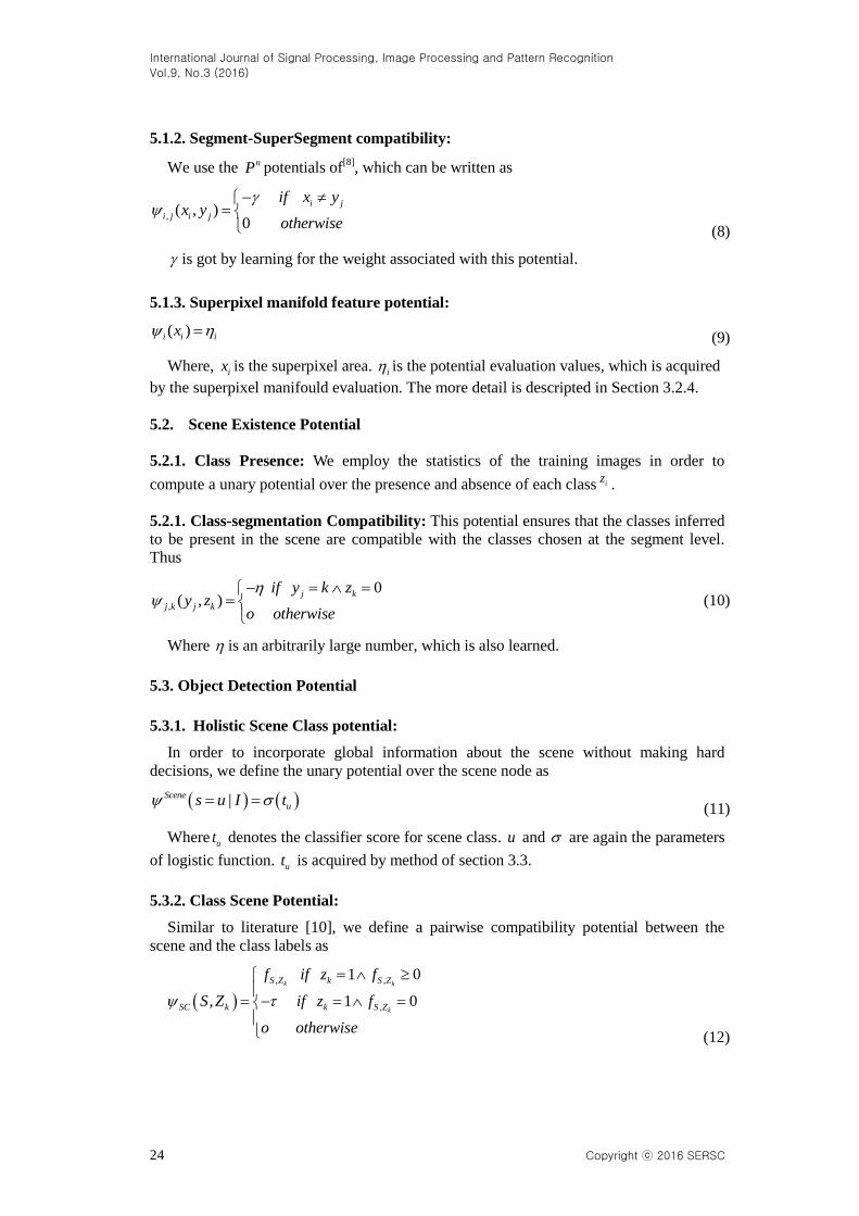
5.1.2. Segment-SuperSegment compatibility:
We use the nP potentials of[8]
, which can be written as
, ( , )0
i j
i j i j
if x yx y
otherwise
(8)
is got by learning for the weight associated with this potential.
5.1.3. Superpixel manifold feature potential:
( )i i ix (9)
Where, ix is the superpixel area. i is the potential evaluation values, which is acquired
by the superpixel manifould evaluation. The more detail is descripted in Section 3.2.4.
5.2. Scene Existence Potential
5.2.1. Class Presence: We employ the statistics of the training images in order to
compute a unary potential over the presence and absence of each class iz .
5.2.1. Class-segmentation Compatibility: This potential ensures that the classes inferred
to be present in the scene are compatible with the classes chosen at the segment level.
Thus
,
0( , )
j k
j k j k
if y k zy z
o otherwise
(10)
Where is an arbitrarily large number, which is also learned.
5.3. Object Detection Potential
5.3.1. Holistic Scene Class potential:
In order to incorporate global information about the scene without making hard
decisions, we define the unary potential over the scene node as
|Scene
us u I t (11)
Where ut denotes the classifier score for scene class. u and are again the parameters
of logistic function. ut is acquired by method of section 3.3.
5.3.2. Class Scene Potential:
Similar to literature [10], we define a pairwise compatibility potential between the
scene and the class labels as
, ,
,
1 0
, 1 0
k k
k
S Z k S Z
SC k k S Z
f if z f
S Z if z f
o otherwise
(12)

International Journal of Signal Processing, Image Processing and Pattern Recognition
Vol.9, No.3 (2016)
Copyright ⓒ 2016 SERSC 25
Where , ks zf represents the probability of occurrence of class kz for scene type s ,
which is estimated empirically from the training data. This potential boosts classes that
frequently co-occur with a scene type, and suppresses the classes that never co-occur with
it.
5.4. Object Detection Potential
We use DPM[29]
to generate candidate object hypotheses. Each object hypothesis
comes with a bounding box, a class, a score and mixture component ID. In order to keep
detections and segmentation coherent, each box lb is connected to the segments
ix that it
intersects with. Furthermore, each lb is connected to z to ensure coherence at the image
level.
5.4.1. Object Candidate Evaluation : We employ DPM[29]
as a detector. It uses a class-
specific threshold that accepts only the highest scoring hypotheses. We reduce these
thresholds to ensure that at least one box per class is available for each image.
1
|0
l l lBBox
cls l
r if b c clsb I
otherwise
(13)
Where, lc is the class of detection,
1
11 exp
x
x
is the logical function.
is the percentage of object regions to bounding box areas of saliency segmentation, which
is acquired by the evaluation values at section 3.4. The reflects the significance of
saliency detection. In our model, we use different evaluation values for each class for
contextual evaluation roles.
5.4.2. Class Detection Compatibility: This term allows the bounding box to be on only
when the class label of that object is also detected as present in the scene. Thus
,
0 1,
0
k l lBClass
l k l k
if z c k bb z
otherwise
(14)
Where is a very large number estimated during learning.
5.4.3. Shape Potential: According to literature [10], , |sh
cls i lx b I is shape potential, each
class has its own.
( ) 1( , | )
i l i lsh
cls i l
x if b x c clsx b I
o otherwise
(15)
Where iA is the set of pixels in the i-th segment, iAis the cardinality of this set, and
( , )lp m is the value of the mean mask for component lm at point p .
5.4.4. Model Learning and Inference: Inference in this model is typically NP-hard. We
rely on approximated algorithms based on LP relaxations. In particular, we employ the
distributed convex belief propagation algorithm[30]
to compute marginal. For learning, we
employ the primal-dual algorithm[22]
and optimize the log-loss. Following literature [10],
we utilize a holistic loss which is the sum of the losses of the individual tasks. Intersection
over union is used for detection, 0-1 loss for classification and pixel-wise labeling for
segmentation

International Journal of Signal Processing, Image Processing and Pattern Recognition
Vol.9, No.3 (2016)
26 Copyright ⓒ 2016 SERSC
Due to the many factors CRF model features formed, we use the large-scale graph
model and distributed message passing algorithm for model reasoning[30]
.
6. Experimental Design
We test our new model on Msrc-v2 data set[2]
for semantic segmentation, object
detection and scene classification.
6.1. Datasets
The detail of Msrc-v2 data set is as shown in Table 1. The Msrc-v2 data set is currently
used for testing the semantic segmentation and classification. The original database
consists of 591 images, of which the statistics of scene classification, semantic annotation
statistics is as shown in Table 1. The number of training set is 335 images, and 256
images for the testing. The image annotation class is the first 7 classes, a total of 22
classes (including the background).
Table 1. The Statistics of Msrc-v2data Set
The class of semantic segmentation The class of scene classification The class of object detection
A total of 22 classes: Building, Grass, Tree,
Cow, Sheep, Sky, Aero plane, Water, Face,
Car, Bicycle, Flower, Sign, Bird, Book, Chair,
Road, Cat, Dog, Body, Boat, Background
A total of 21 classes: Sign, Bir, Dog,
Cat, Bicycle, Tree, Water, Sheep, Perso,
Building, Cow, Chai, Aero plane, Grass,
City, Flower, Book, Boat, Nature, Car,
Face
A total of 15 classes: Cow, Sheep,
Aero plane, Face, Car, Bicycle,
Flower, Sign, Bird, Book, Chair,
Cat, Dog, Body, Boat
6.2. Experimental Platforms
We test our model on the Msrc-v2 dataset. The testing hardware environment is the
CPU of Intel P6100, 2.00 GHZ and memory of 6 GB RAM. Our development and testing
platform is Ubuntu12.04 operating system with Matlab2013b and gc ++ development.
6.3. Experimental Settings
In order to compare to literature [10], our testing setting is same as literature [10].
1) Superpixel size
There is a threshold for UCM [26]
. In our experiments we set the threshold to be 0.08
and 0.16 for the two layers in the hierarchy of MSRC-21 data set. The number and size of
the output regions is range from 22 to 65.
2) Object detection
Our method is same as literature [29] for object detection.
3) Evaluation method
The evaluation method is similar to literature [20] as shown in Figure 5.
In the sub-graph (a), gtB is the bounding box of ground truth, dtB is the bounding box of
detection value. The overlapping of ,gt dtB B is computed as formulation 16.
( , ) 0.5gt dt
gt dt
gt dt
B BB B
B B
Over l appi ng (16)
International Journal of Signal Processing, Image Processing and Pattern Recognition
Vol.9, No.3 (2016)
Copyright ⓒ 2016 SERSC 27
Groundtruth
Detection
Overlap( , )
gtB
dtB
gtBdtB
(a) (b)
0 0.5 10
0.2
0.4
0.6
0.8
1
recall
pre
cisi
on
PR (AP: 93.26%)
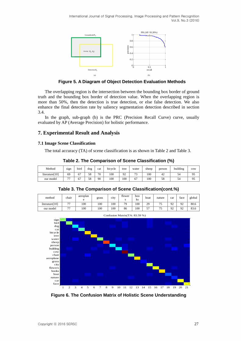
Figure 5. A Diagram of Object Detection Evaluation Methods
The overlapping region is the intersection between the bounding box border of ground
truth and the bounding box border of detection value. When the overlapping region is
more than 50%, then the detection is true detection, or else false detection. We also
enhance the final detection rate by saliency segmentation detection described in section
3.4.
In the graph, sub-graph (b) is the PRC (Precision Recall Curve) curve, usually
evaluated by AP (Average Precision) for holistic performance.
7. Experimental Result and Analysis
7.1 Image Scene Classification
The total accuracy (TA) of scene classification is as shown in Table 2 and Table 3.
Table 2. The Comparison of Scene Classification (%)
Method sign bird dog cat bicycle tree water sheep person building cow
literature[10] 69 67 58 70 100 92 73 100 42 54 95
our model 77 67 58 90 100 100 67 100 58 54 95
Table 3. The Comparison of Scene Classification(cont.%)
method chair aeroplan
e grass city
flower
s
boo
ks boat nature car face global
literature[10] 77 100 100 100 79 100 29 75 92 92 80.6
our model 77 100 100 100 86 100 57 75 92 92 83.6
Confusion Matrix(TA: 83.59 %)
1 2 3 4 5 6 7 8 9 10 11 12 13 14 15 16 17 18 19 20 21
sign
bird
dog
cat
bicycle
tree
water
sheep
person
building
cow
chair
aeroplane
grass
city
flowers
books
boat
nature
car
face
Figure 6. The Confusion Matrix of Holistic Scene Understanding

International Journal of Signal Processing, Image Processing and Pattern Recognition
Vol.9, No.3 (2016)
28 Copyright ⓒ 2016 SERSC
From Table 2 and Table 3, we can see that:
1) From the total classification accuracy, our model is apparently superior to
literature [10] that the total accuracy is boosted from 80.6% to 83.6%.
2) For each class accuracy, except water and flower, the other class is better or at least
same as literature [10]. The classes of performance boosted greatly are cat class from 70%
to 90%, person from 42% to 58%, boat from 29% to 57%.
3) As shown before, it’s implicitly effective to add global information for better scene
classification.
4) The Figure 6 is the confusion matrix for scene classification. We clearly see
erroneous classification of each class. For example, the sign class has been misclassified
as bird, building and city.
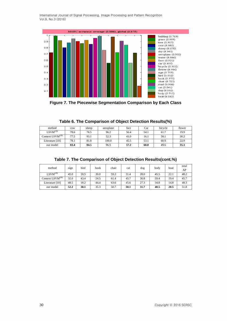
7.2 Image Semantic Segmentation
The comparisons of each classification accuracy, average accuracy and global
accuracy of semantic segmentation is shown in Table 4 and Table 5. The Figure 7 is the
piecewise segmentation comparison by each class. From Table 4, 5 and Figure 7, we can
see that:
1) From the global semantic segmentation accuracy in terms of our model compared
with literature [10] The model has been some improvement, increased from 86.2% to
87.5%, an increase of 1.3%.
2) From the circumstances of each classification accuracy rate of view, our model is
beyond literature [10] The accuracy rate in each class, of course, the overall rate of
increase is still relatively small.
3) From the above analysis, we can see two images of popular features to increase the
information we put forward to improve the semantic segmentation is effective.
Figure 7 is the piecewise segmentation comparison by each class. From Figure 7, we
can clearly see that the semantic segmentation accuracy of each class, the highest of
which is 98.9% of grass, of the lowest is 18.3% of the ship.
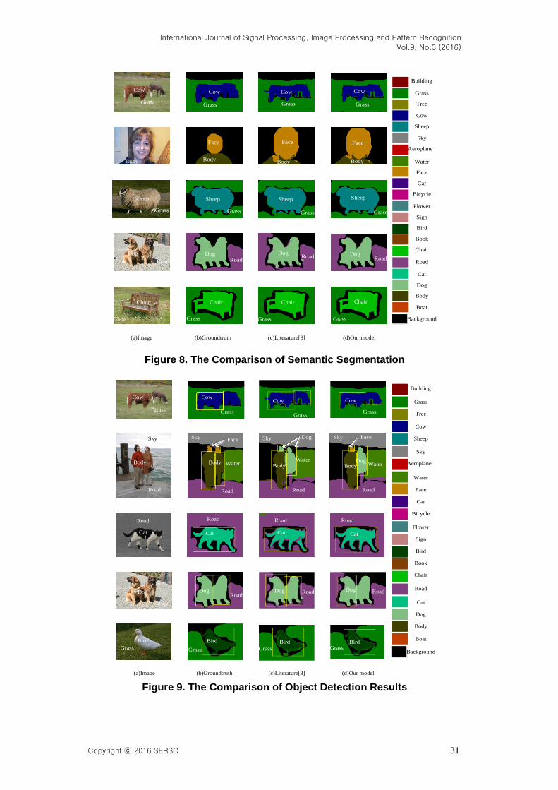
Figure 8, the column (a) is the original image, the column (b) is the ground truth of
the data set, the column (c) is segmentation results of a literature [10], the column (d) is
segmentation results of our model.
From the Figure 8, we can more clearly see that our model semantic segmentation is
significantly better than the original literature [10] model at the corners and edges. For
example, at the first line, our model does not have the ox tail, which is consistent with the
ground truth. On the second line, the head and hair part of neck in our model is
significantly better than that of literature [10]. The last three lines are mainly some
improvements in fine detail.
7.3 Object Detection
The comparison of average accuracy by each class and total precision accuracy for
object detection is shown in Table 6 and Table 7 below. From Table 6 and Table 7, we can
see that:
1) The object detection accuracy of our model compared with literature [10] is
increased from 49.3% to 51.8%, an increase of 1.5%.
2) In the detection classes of cows, sheep, face, cars, flowers, logo, birds, cats, dogs,
humans and the boat, our model goes beyond the model of literature [10]. The accuracy
performance, cow increases from 78.1% to 83.4%, an increase of 5.3%, sheep from 81.8
to 84.5%, an increase of 2.7%, human face from 45.5 percent to 57.2, an increase of
11.7%, cars from 53.1% to 60%, an increase of 6.9 %, flowers from 22.9% to 35.3%, an
increase of 12.4%, sign from 48.5% to 52.2%, an increase of 3.7%, birds from 18.2% to
30.1%, an increase of 11.9%; cat from 45.6% to 50.1%, an increase of 4.5%, dogs from
27.3% to 31.7%, an increase of 4.4%, the body from 34.8% to 40.5%, an increase of
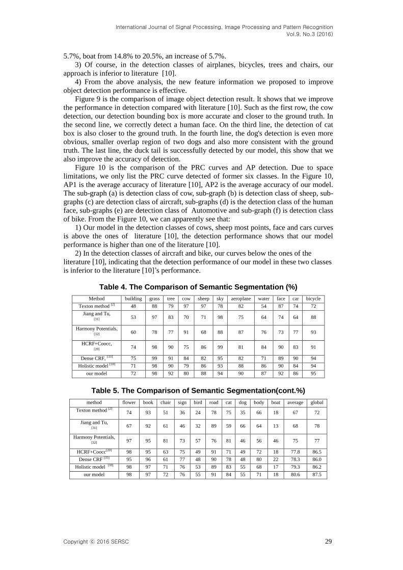
International Journal of Signal Processing, Image Processing and Pattern Recognition
Vol.9, No.3 (2016)
Copyright ⓒ 2016 SERSC 29
5.7%, boat from 14.8% to 20.5%, an increase of 5.7%.
3) Of course, in the detection classes of airplanes, bicycles, trees and chairs, our
approach is inferior to literature [10].
4) From the above analysis, the new feature information we proposed to improve
object detection performance is effective.
Figure 9 is the comparison of image object detection result. It shows that we improve
the performance in detection compared with literature [10]. Such as the first row, the cow
detection, our detection bounding box is more accurate and closer to the ground truth. In
the second line, we correctly detect a human face. On the third line, the detection of cat
box is also closer to the ground truth. In the fourth line, the dog's detection is even more
obvious, smaller overlap region of two dogs and also more consistent with the ground
truth. The last line, the duck tail is successfully detected by our model, this show that we
also improve the accuracy of detection.
Figure 10 is the comparison of the PRC curves and AP detection. Due to space
limitations, we only list the PRC curve detected of former six classes. In the Figure 10,
AP1 is the average accuracy of literature [10], AP2 is the average accuracy of our model.
The sub-graph (a) is detection class of cow, sub-graph (b) is detection class of sheep, sub-
graphs (c) are detection class of aircraft, sub-graphs (d) is the detection class of the human
face, sub-graphs (e) are detection class of Automotive and sub-graph (f) is detection class
of bike. From the Figure 10, we can apparently see that:
1) Our model in the detection classes of cows, sheep most points, face and cars curves
is above the ones of literature [10], the detection performance shows that our model
performance is higher than one of the literature [10].
2) In the detection classes of aircraft and bike, our curves below the ones of the
literature [10], indicating that the detection performance of our model in these two classes
is inferior to the literature [10]’s performance.
Table 4. The Comparison of Semantic Segmentation (%)
Method building grass tree cow sheep sky aeroplane water face car bicycle
Texton method [2]
48 88 79 97 97 78 82 54 87 74 72
Jiang and Tu, [31]
53 97 83 70 71 98 75 64 74 64 88
Harmony Potentials, [32]
60 78 77 91 68 88 87 76 73 77 93
HCRF+Coocc, [20]
74 98 90 75 86 99 81 84 90 83 91
Dense CRF, [33]
75 99 91 84 82 95 82 71 89 90 94
Holistic model [10]
71 98 90 79 86 93 88 86 90 84 94
our model 72 98 92 80 88 94 90 87 92 86 95
Table 5. The Comparison of Semantic Segmentation(cont.%)
method flower book chair sign bird road cat dog body boat average global
Texton method [2]
74 93 51 36 24 78 75 35 66 18 67 72
Jiang and Tu, [31]
67 92 61 46 32 89 59 66 64 13 68 78
Harmony Potentials, [32]
97 95 81 73 57 76 81 46 56 46 75 77
HCRF+Coocc[20]
98 95 63 75 49 91 71 49 72 18 77.8 86.5
Dense CRF [33]
95 96 61 77 48 90 78 48 80 22 78.3 86.0
Holistic model [10]
98 97 71 76 53 89 83 55 68 17 79.3 86.2
our model 98 97 72 76 55 91 84 55 71 18 80.6 87.5
International Journal of Signal Processing, Image Processing and Pattern Recognition
Vol.9, No.3 (2016)
30 Copyright ⓒ 2016 SERSC
Figure 7. The Piecewise Segmentation Comparison by Each Class
Table 6. The Comparison of Object Detection Results(%)
method cow sheep aeroplane face Car bicycle flower
LSVM[29]
78.6 76.5 96.2 56.4 54.1 61.7 19.9
Context LSVM[29]
77.5 93.1 52.3 41.0 16.1 58.1 30.2
Literature [10] 78.1 81.8 100.0 45.5 53.1 60.9 22.9
our model 83.4 84.5 96.5 57.2 60.0 49.6 35.3
Table 7. The Comparison of Object Detection Results(cont.%)
method sign bird book chair cat dog body boat total
AP
LSVM[29]
45.0 18.5 30.0 59.2 31.4 28.0 45.5 22.1 48.2
Context LSVM[29]
32.0 43.4 24.5 61.4 45.7 30.8 59.4 19.4 45.7
Literature [10] 48.5 18.2 44.4 63.6 45.6 27.3 34.8 14.8 49.3
our model 52.2 30.1 35.3 50.7 50.1 31.7 40.5 20.5 51.8
International Journal of Signal Processing, Image Processing and Pattern Recognition
Vol.9, No.3 (2016)
Copyright ⓒ 2016 SERSC 31
(a)Image (b)Groundtruth (c)Literature[8] (d)Our model
Cow Cow Cow Cow
GrassGrassGrassGrass
Body Body Body
FaceFaceFaceFace
Body
Sheep Sheep Sheep Sheep
GrassGrassGrassGrass
DogDogDogDog
Chair Chair Chair Chair
GrassGrassGrassGrass
Road RoadRoad Road
Building
Grass
Tree
Cow
Sheep
Aeroplane
Sky
Water
Face
Car
Bicycle
Flower
Sign
Bird
Book
Chair
Road
Cat
Dog
Body
Boat
Background
Figure 8. The Comparison of Semantic Segmentation
Figure 9. The Comparison of Object Detection Results
(a)Image (b)Groundtruth (c)Literature[8] (d)Our model
Building
Grass
Tree
Cow
Sheep
Aeroplane
Sky
Water
Face
Car
Bicycle
Flower
Sign
Bird
Book
Chair
Road
Cat
Dog
Body
Boat
Background
GrassGrass
Grass
Grass Grass GrassGrass
grass
Bird Bird Bird Bird
DogDogDogDog
Dog
Dog
Road
RoadRoad Road
Road RoadRoadRoad
Road Road Road Road
BodyBodyBodyBody
SkySkySkySky
CowCowCowCow
FaceFace
WaterWater
Water
Cat Cat Cat Cat
Face

International Journal of Signal Processing, Image Processing and Pattern Recognition
Vol.9, No.3 (2016)
32 Copyright ⓒ 2016 SERSC
(a) (b)
(c) (d)
(e) (f)
Figure 10. The Comparison of PRC Curve of Six Classes Object Detection

International Journal of Signal Processing, Image Processing and Pattern Recognition
Vol.9, No.3 (2016)
Copyright ⓒ 2016 SERSC 33
7.4 The Impact Analysis of Mask Size
In section 4.2.4 the size of mask square will affect the final results. We tested the
final segmentation semantic influence by different mask sizes, as shown in Table 8.
Table 8. The Impact Analysis of Mask Size
Mask size 2 2 3 3 4 4 5 5 6 6 7 7 8 8 9 9 10 10
Total accuracy(%) 85.4 86.0 86.6 87.5 87.4 87.5 87.5 87.3 87.1
From Table 8 we can find that, with the increase of the mask size, the overall accuracy
increases at the initial stage, but the increasing tendency is stopped at the size of 5 5, and
then begin to decrease when the mask size is 6 6. The phenomenon shows that it’s not
always effective for increase the mask size. So in our study, we selected 5 5 as the
default mask size.
8 Conclusion and future work
For the image feature engineering problems of overall understanding based on
conditional random fields, we propose methods to improve the classification performance
based on PHOW and KPCA dimensionality reduction characteristics, significantly
improve segmentation and semantic segmentation by image manifold features and
saliency segmentation. The experiments show that the proposed model has higher overall
performance compared with literature [10] in three areas of scene classification, semantic
segmentation and object detection. We summarize as follows:
1) Scene Classification: This paper studies feature fusion problem of the holistic scene
model. We propose the feature transformation method based on PHOW feature with
KPCA kernel transformation which effectively reduces the dimension processing features,
but without losing accuracy. The experiments show that the accuracy of the overall
classification increased from the original 80.6% to 83.6%, an increase of 2%.
2) Semantic Segmentation: We use two ways to improve the model performance (1)
new unary potential by incorporating HOG features, LBP features and RGB color
histogram feature information to enhance the classifier training; (2) adding higher order
potential to reflect the image inherent manifold features. The experiments show that the
overall performance of the semantic segmentation is increased from the original 86.2% to
87.5%, an increase of 1.3%.
3) Object detection: We propose a method to improve the object detection results by
more accurately selecting the detection bounding box based on saliency segmentation
information. The Experiments show that the integrity of the object detection is increased
from the original 49.3% to 51.8%, an increase of 1.5%.
Lastly, to conclude, the future issues are described below:
1) The only way for holistic scene understanding is to adopt a more rational and
reasonable architecture. Because, there are many factors affecting the holistic scene
understanding, and having the mutual influence and constraints. The model framework
with rational and scientific consideration will directly affect the performance of the
holistic scene understanding.
2) We need more in-depth or more appropriate theory to reveal the relationship within
the image for holistic scene understanding by probabilistic graphical models. This has a
long way to go.
3) The development of the image holistic scene understanding depends on people's
further understanding of cognitive theory. Because it’s a very simple understanding for the
people, but machine requires very complex calculation process, how to use the computer
to represent and simulate human holistic scene understanding is particularly important.
4) Both directed graph and undirected graph have demonstrated their success in image
International Journal of Signal Processing, Image Processing and Pattern Recognition
Vol.9, No.3 (2016)
34 Copyright ⓒ 2016 SERSC
understanding, each has its own advantages and disadvantages. The combination of
Bayesian model base on directed graph and CRF based on undirected graph model is the
more rational and effective way to understand the nature scene and reveal the holistic
image characteristics. This should be worthy of further exploration.
Acknowledgements
This work was supported in part by the Scientific Research Fund of Sichuan
Provincial Education Department of China (No. 15TD0038).
References [1] L. Li, Y. Wu and M. Ye, "A New Framework for Direct Saliency Detection and Segmentation Based on
Graph Methods[J]", International Journal of Signal Processing, Image Processing and Pattern
Recognition, vol. 7, no. 1, (2014), pp. 379-392.
[2] J. Shotton, J. Winn and C. Rother, "Textonboost: Joint appearance, shape and context modeling for
multi-class object recognition and segmentation[C]", Proceedings of the 9th European Conference on
Computer Vision, ECCV, Graz, Austria, (2006), pp. 1-15.
[3] J. Besag, "Spatial interaction and the statistical analysis of lattice systems[J]", Journal of the Royal
Statistical Society. Series B (Methodological), (1974), vol. 36, no. 2, pp. 192-236.
[4] R. Szeliski, "Computer vision: Algorithms and applications[M]", Germany: Springer, (2010), pp. 11-19.
[5] C. Wang, N. Komodakis and N. Paragios, "Markov Random Field modeling, inference & learning in
computer vision & image understanding: A survey[J]", Computer Vision and Image Understanding,
(2013), vol. 117, no. 11, pp. 1610-1627.
[6] K. Park and S. Gould, "On learning higher-order consistency potentials for multi-class pixel
labeling[C]", Proceedings of the 12th European Conference on Computer Vision–ECCV 2012, Florence,
Italy, (2012), pp. 202-215.
[7] S. Gould, T. Gao and D. Koller, "Region-based Segmentation and Object Detection[C]", Proceedings of
the Advances in Neural Information Processing Systems, Vancouver, BC, Canada, (2009), pp. 655-663.
[8] P. Kohli, M. P. Kumar and P. H. Torr, "P3 & beyond: Solving energies with higher order cliques[C]",
Proceedings of the 2007 IEEE Computer Society Conference on Computer Vision and Pattern
Recognition, Minneapolis, MN, United states, (2007), pp. 1-8.
[9] V. Vineet, C. Rother and P. Torr, "Higher Order Priors for Joint Intrinsic Image, Objects, and Attributes
Estimation[C]", Proceedings of the Advances in Neural Information Processing Systems, Lake Tahoe,
Nevada, United States, (2013), pp. 557-565.
[10] J. Yao, S. Fidler and R. Urtasun,. "Describing the scene as a whole: Joint object detection, scene
classification and semantic segmentation[C]", Proceedings of the 2012 IEEE Conference on Computer
Vision and Pattern Recognition, Providence, RI, United states, (2012), pp. 702-709.
[11] P. Kohli, L. Ladicky and P. Torr, "Graph cuts for minimizing robust higher order potentials[J]",
International Journal of Computer Vision, vol. 82, no. 3, (2009), pp. 302-324.
[12] P. Kohli and P. H. Torr, "Robust higher order potentials for enforcing label consistency[J]",
International Journal of Computer Vision, vol. 82, no. 3, (2009), pp. 302-324.
[13] D. Lin, S. Fidler and R. Urtasun, "Holistic scene understanding for 3d object detection with rgbd
cameras[C]", Proceedings of the 14th IEEE International Conference on Computer Vision, Sydney,
NSW, Australia, (2013), pp. 1417-1424.
[14] R. Mottaghi, S. Fidler and J. Yao, "Analyzing Semantic Segmentation Using Hybrid Human-Machine
CRFs[C]", Proceedings of the 26th IEEE Conference on Computer Vision and Pattern Recognition,
Portland, OR, United states, (2013), pp. 3012-3019.
[15] H. G. Barrow and J. M. Tenenbaum, "Recovering Intrinsic Scene Characteristics from Images[M]",
(1978), pp. 3-26.
[16] A. Torralba, K. P. Murphy and W. T. Freeman, "Contextual Models for Object Detection Using Boosted
Random Fields[C]", Proceedings of the Advances in neural information processing systems, Vancouver,
BC, Canada, (2004), pp. 1401-1408.
[17] S. Kumar and M. Hebert, "A hierarchical field framework for unified context-based classification[C]",
Proceedings of the 10th IEEE International Conference on Computer Vision, ICCV 2005, Beijing,
China, (2005), pp. 1284-1291.
[18] A. Rabinovich, A. Vedaldi and C. Galleguillos, "Objects in context[C]", Proceedings of the 11th IEEE
International Conference on Computer vision, ICCV 2007, Janeiro, Brazil, (2007), pp. 1-8.
[19] C. Liu, J. Yuen and A. Torralba, "Nonparametric scene parsing: Label transfer via dense scene
alignment[C]", Proceedings of the IEEE Conference on 2009 Computer Vision and Pattern Recognition,
Miami, FL, United states, (2009), pp. 1972-1979.
International Journal of Signal Processing, Image Processing and Pattern Recognition
Vol.9, No.3 (2016)
Copyright ⓒ 2016 SERSC 35
[20] Ľ. Ladický, P. Sturgess and K. Alahari, "What, where and how many? combining object detectors and
crfs[C]", Proceedings of the 11th European Conference on Computer Vision, ECCV 2010, Heraklion,
Crete, Greece, (2010), pp. 424-437.
[21] C. Wojek and B. Schiele, "A dynamic conditional random field model for joint labeling of object and
scene classes[C]", Proceedings of the 9th European Conference on Computer Vision, ECCV 2008,
Marseille, France, (2008), pp. 733-747.
[22] T. Hazan and R. Urtasun, "A primal-dual message-passing algorithm for approximated large scale
structured prediction[C]", Proceedings of the Advances in Neural Information Processing Systems,
Vancouver, BC, Canada, (2010), pp. 838-846.
[23] L. Li, J. Lian and Y. Wu, "Image Classification Based on KPCA and SVM with Randomized Hyper-
parameter Optimization[J]", International Journal of Signal Processing, Image Processing and Pattern
Recognition, vol. 7, no. 4, (2014), pp. 303-316.
[24] A. Torralba, K. P. Murphy and W. T. Freeman, "Sharing features: efficient boosting procedures for
multiclass object detection[C]", Proceedings of the Proceedings of the 2004 IEEE Computer Society
Conference on Computer Vision and Pattern Recognition., Washington, DC, USA, (2004), pp. 762-769.
[25] S. Brin and L. Page, "The anatomy of a large-scale hypertextual Web search engine[J]", Computer
networks and ISDN systems, vol. 30, no. 1, (1998), pp. 107-117.
[26] P. Arbelaez, M. Maire and C. Fowlkes, "Contour detection and hierarchical image segmentation[J]",
IEEE Transactions on Pattern Analysis and Machine Intelligence, vol. 33, no. 5, (2011), pp. 898-916.
[27] C. Yang, L. Zhang and H. Lu, "Saliency Detection via Graph-Based Manifold Ranking[C]",
Proceedings of the 2013 IEEE Conference on Computer Vision and Pattern Recognition (CVPR),
Portland, OR, United states, (2013), pp. 3166-3173.
[28] D. Zhou, J. Weston and A. Gretton, "Ranking on data manifolds[C]", Proceedings of the Advances in
Neural Information Processing Systems, Whistler, British Columbia, Canada, (2003), pp. 398-405.
[29] P. F. Felzenszwalb, R. B. Girshick and D. McAllester, "Object detection with discriminatively trained
part-based models[J]", IEEE Transactions on Pattern Analysis and Machine Intelligence, vol. 32, no. 9,
(2010), pp. 1627-1645.
[30] A. Schwing, T. Hazan and M. Pollefeys, "Distributed message passing for large scale graphical
models[C]", Proceedings of the 2011 IEEE Conference on Computer Vision and Pattern Recognition
(CVPR), Colorado Springs, CO, United States, (2011), pp. 1833-1840.
[31] J. Jiang and Z. Tu, "Efficient scale space auto-context for image segmentation and labeling[C]",
Proceedings of the IEEE Conference on Computer Vision and Pattern Recognition, CVPR 2009, Miami,
FL, United States,( 2009), pp. 1810-1817.
[32] J. M. Gonfaus, X. Boix and J. Van De Weijer, "Harmony potentials for joint classification and
segmentation[C]", Proceedings of the 2010 IEEE Conference on Computer Vision and Pattern
Recognition (CVPR), San Francisco, CA, United states, (2010), pp. 3280-3287.
[33] P. Krähenbühl, V. Koltun. Efficient inference in fully connected crfs with gaussian edge potentials[C].
Proceedings of the Advances in Neural Information Processing Systems, Lake Tahoe, Nevada, USA,
(2012), pp. 406-414.
Authors
Lin Li, He is a Ph.D and an associate professor at department of
Computer Science and technology, Chengdu Normal University.
He is also a system analyser of computer and software technology
of P.R. China and member of China Computer Federation. His
research interest covers machine learning and its application in
image processing and computer vision. He is the corresponding
author of this paper.

International Journal of Signal Processing, Image Processing and Pattern Recognition
Vol.9, No.3 (2016)
36 Copyright ⓒ 2016 SERSC