Image formation and fundamentals - Università degli Studi di … · 2009-02-03 · – CMOS...
52
1 Image formation and fundamentals
Transcript of Image formation and fundamentals - Università degli Studi di … · 2009-02-03 · – CMOS...

1
Image formation and fundamentals

2
IP frameworkNatural scene Digital image
15 25 44 100
Image Processing
System
filteringtransformscoding....
Image rendering
capturesamplingquantizationcolor space
Is this good quality
How can I protect
my data?
What is the best I can get over my
phone line?
How much will it cost?
NetworkNetwork

3
IP: basic steps
{15,1,2} {25,44,1}….
A/D conversion
Sampling (2D) Quantization
Analog image
Digital image
(capturing device)

4
Digital Image AcquisitionSensor array
• When photons strike, electron-hole pairs are generated on sensor sites.
• Electrons generated are collected over a certain period of time.
• The number of electrons are converted to pixel values. (Pixel is short for picture element.)

5
Object(surface element)
Surface reflectance Radiance
Optical axis
Light source
N
IrradianceCAMERA
Sensors
theta
Image capture
VM1

Slide 5
VM1 - radianza: energia che viene emessa dall'elemento di superficie- irradianza: energia che colpisce la camera e dipende da lo spettro della luce, la riflettanza della superficie (che cambia lo spettro) e la sensibilità spettraledel sensoreswan; 14/01/2004

6
Digital Image Acquisition
Two types of discretization:1. There are finite number of pixels.
(sampling → Spatial resolution)2. The amplitude of pixel is
represented by a finite number of bits. (Quantization → Gray-scale resolution)

7
Digital Image Acquisition
Take a look at this cross section

8
Digital Image Acquisition
• 256x256 - Found on very cheap cameras, this resolution is so low that the picture quality is almost always unacceptable. This is 65,000 total pixels.
• 640x480 - This is the low end on most "real" cameras. This resolution is ideal for e-mailing pictures or posting pictures on a Web site.
• 1216x912 - This is a "megapixel" image size -- 1,109,000 total pixels -- good for printing pictures.
• 1600x1200 - With almost 2 million total pixels, this is "high resolution." You can print a 4x5 inch print taken at this resolution with the same quality that you would get from a photo lab.
• 2240x1680 - Found on 4 megapixelcameras -- the current standard -- this allows even larger printed photos, with good quality for prints up to 16x20 inches.
• 4064x2704 - A top-of-the-line digital camera with 11.1 megapixels takes pictures at this resolution. At this setting, you can create 13.5x9 inch prints with no loss of picture quality.
9
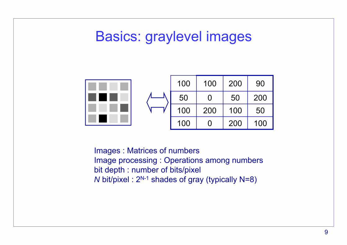
Basics: graylevel images
10020001005010020010020050050
90200100100
Images : Matrices of numbersImage processing : Operations among numbersbit depth : number of bits/pixelN bit/pixel : 2N-1 shades of gray (typically N=8)
10
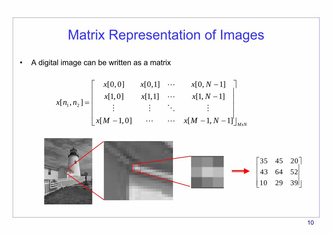
Matrix Representation of Images
• A digital image can be written as a matrix
1 2
[0, 0] [0,1] [0, 1][1, 0] [1,1] [1, 1]
[ , ]
[ 1, 0] [ 1, 1] MxN
x x x Nx x x N
x n n
x M x M N
−⎡ ⎤⎢ ⎥−⎢ ⎥=⎢ ⎥⎢ ⎥− − −⎣ ⎦
35 45 2043 64 5210 29 39
⎡ ⎤⎢ ⎥⎢ ⎥⎢ ⎥⎣ ⎦

11
Digital images acquisition
• Analog camera+A/D converter
• Digital cameras– CCDs (Charge Coupled Devices)– CMOS technology
• In both cases: optics– lenses, diaphrams
Matrices of photo sensors collecting photons of given wavelength
Features of the capture devices:
• Size and number of photosites• Noise• Transfer function of the optical filter

12
Color images
• Each colored pixel corresponds to a vector of three values {C1,C2,C3}
• The characteristics of the components depend on the chosen colorspace (RGB, YUV, CIELab,..)
C1 C2 C3

13
Digital Color Images
• 1 2[ , ]Rx n n1 2[ , ]Gx n n1 2[ , ]Bx n n

14
Color channels
Red Green Blue

15
Color channels
Red Green Blue

16
The physical perspective

17
The perceptual perspective
Simultaneous contrast

18
Color
• Chromatic induction

19
Color
• Human vision– Color encoding (receptor level)– Color perception (post-receptoral
level)– Color semantics (cognitive level)
• Colorimetry– Spectral properties of radiation– Physical properties of materials
Color vision(Seeing colors)
Colorimetry(Measuring colors)
Color categorization and naming (understanding
colors)
MODELS

20
Bayer matrix
Typical sensor topology in CCD devices. The green is twice as numerous as red and blue.

21
Displays
LCD
CRT

22
Color Displays
CRT
LCD
Polarize to control the amount of light passed.

23
Color imaging
• Color reproduction– Printing, rendering
• Digital photography– High dynamic range images– Mosaicking– Compensation for differences in illuminant (CAT: chromatic adaptation
transforms)
• Post-processing– Image enhancement
• Coding– Quantization based on color CFSs (contrast sensitivity function)– Downsampling of chromatic channels with respect to luminance

24
Some definitions
• Digital images– Sampling+quantization
• Sampling– Determines the graylevel value of each pixel
• Pixel = picture element
• Quantization– Reduces the resolution in the graylevel value to that set by the
machine precision
• Images are stored as matrices of unisigned chars

25
Resolution
• Sensor resolution (CCD): Dots Per Inch (DPI)– Number of individual dots that can be placed within the span of one linear inch
(2.54 cm)
• Image resolution– Pixel resolution: NxM– Spatial resolution: Pixels Per Inch (PPI)– Spectral resolution: bandwidth of each spectral component of the image
• Color images: 3 components (R,G,B channels)• Multispectral images: many components (ex. SAR images)
– Radiometric resolution: Bits Per Pixel (bpp)• Graylevel images: 8, 12, 16 bpp• Color images: 24bpp (8 bpp/channel)
– Temporal resolution: for movies, number of frames/sec• Typically 25 Hz (=25 frames/sec)
VM2

Slide 25
VM2 da book Shapiroswan; 10/04/2003

26
Example: pixel resolution

27
Image ResolutionDon’t confuse image size and resolution.
28
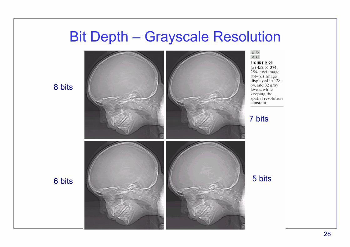
Bit Depth – Grayscale Resolution
8 bits
7 bits
6 bits 5 bits

29
Bit Depth – Grayscale Resolution4 bits
3 bits
2 bits 1 bit

30
File format
• Many image formats (about 44)
• BMP, lossless
• TIFF, lossless/lossy
• GIF (Graphics Interchange Format)– Lossless, 256 colors, copyright protected
• JPEG (Joint Photographic Expert Group)– Lossless and lossy compression– 8 bits per color (red, green, blue) for a 24-bit total
• PNG (Portable Network Graphics)– Freewere– supports truecolor (16 million colours)

31
Sampling in 2D

32
Sampling in 1D
t
f(t)
( )[ ] ( ) ( )s sk
f k f kT f t t kTδ= = −∑
k
f(t)
Continuous time signal
Discrete time signal
comb

33
Nyquist theorem (1D)
At least 2 sample/period are needed to represent a periodic signal
max
max
1 222 2
s
ss
T
T
πωπω ω
≤
= ≥

34
Delta pulse

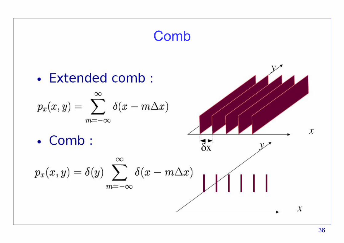
35
Dirac brush
36
Comb

37
Brush

38
Nyquist theorem
• Sampling in p-dimensions
• Nyquist theorem
)()()(
)()(
xsxfxf
kTxxs
TT
ZkT
p
=
−= ∑∈
δTs
y
2D spatial domain
2D Fourier domain
ω x
ωy
ωxmax
ωymax
max max
max
max
122 2
12 22
sxs
x x xs
sy yy
y
T
T
πω ω ωω ω π
ω
⎧ ≤⎪⎧ ≥⎪ ⎪⇒⎨ ⎨≥⎪⎩ ⎪ ≤⎪⎩
Tsx

39
Spatial aliasing

40
Resampling
• Change of the sampling rate– Increase of sampling rate: Interpolation or upsampling
• Blurring, low visual resolution– Decrease of sampling rate: Rate reduction or downsampling
• Aliasing and/or loss of spatial details

41
Downsampling

42
Upsampling
nearest neighbor (NN)

43
Upsampling
bilinear

44
Upsampling
bicubic

45
Quantization

46
Quantization
• A/D conversion quantization
Quantizer
f in L2(R) discrete functionf in L2(Z)
fq=Q{f}
ftk tk+1
uniform perceptual
rk
fq=Q{f}
fThe sensitivity of the eye decreases increasing the background intensity (Weber law)

47
QuantizationSignal before (blue) and after quantization (red) Q
Equivalent noise: n=fq- f
additive noise model: fq=f+n

48
Quantization
original 5 levels
10 levels 50 levels

49
Distortion measure
• Distortion measure
– The distortion is measured as the expectation of the mean square error (MSE) difference between the original and quantized signals.
• Lack of correlation with perceived image quality– Even though this is a very natural way for the quantification of the quantization
artifacts, it is not representative of the visual annoyance due to the majority of common artifacts.
• Visual models are used to define perception-based image quality assessment metrics
( )[ ] ( )∑ ∫=
+
−=−Ε=K
k
t
tQQ
k
k
dffpffffD0
221
)(

50
Example
• The PSNR does not allow to distinguish among different types of distortions leading to the same RMS error between images
• The MSE between images (b) and (c) is the same, so it is the PSNR. However, the visual annoyance of the artifacts is different