Image De-noising by Various Filters for Different Noise using MATLAB Winter Training 2012

Mentor-Mr. MANJEET KUMAR

Submitted By-Jitesh Gupta(54/EC/10)

Karan Choudhary(56/EC/10)

Kovil Singh(57/EC/10)

ABSTRACT Image processing is basically the use of computer algorithms to perform image processing on digital images. Digital image processing is a part of digital signal processing. Digital image processing has many significant advantages over analog image processing. Image processing allows a much wider range of algorithms to be applied to the input data and can avoid problems such as the build-up of noise and signal distortion during processing of images. Wavelet transforms have become a very powerful tool for de-noising an image. One of the most popular methods is wiener filter. In this report four types of noise (Gaussian noise , Salt & Pepper noise, Speckle noise and Poisson noise) is used and image de-noising performed for different noise by Mean filter, Median filter and Wiener filter . Further results have been compared for all noises.

INTRODUCTION Image de-noising is an vital image processing task i.e. as a process itself as well as a component in other processes. There are many ways to de-noise an image or a set of data and methods exists. The important property of a good image denoising model is that it should completely remove noise as far as possible as well as preserve edges. Traditionally, there are two types of models i.e. linear model and non-liner model. Generally, linear models are used. The benefits of linear noise removing models is the speed and the limitations of the linear models is, the models are not able to preserve edges of the images in a efficient manner i.e the edges, which are recognized as discontinuities in the image, are smeared out. On the other hand, Non-linear models can handle edges in a much better way than linear models. One popular model for nonlinear image denoising is the Total Variation (TV)-filter.We suggest to de-noise a degraded image X given by X = S + N, where S is the original image and N is an Additive White Gaussian noise with unknown variance.

MEAN FILTER We can use linear filtering to remove certain types of noise. Certain filters, such as averaging or Gaussian filters, are appropriate for this purpose. For example, an averaging filter is useful for removing grain noise from a photograph. Because each pixel gets set to the average of the pixels in its neighborhood, local variations caused by grain are reduced. Conventionally linear filtering Algorithms were applied for image processing. The fundamental and the simplest of these algorithms is the Mean Filter .The Mean Filter is a linear filter which uses a mask over each pixel in the signal. Each of the components of the pixels which fall under the mask are averaged together to form a single pixel. This filter is also called as average filter. The Mean Filter is poor in edge preserving.The Mean Filter can be defined as- Mean filter (x1…..xN) = ─ Σ xi/N where (x1 ….. xN) is the image pixel range. Generally linear filters are used for noise suppression.

The idea of mean filtering is simply to replace each pixel value in an image with the mean (`average') value of its neighbors, including itself. This has the effect of eliminating pixel values which are unrepresentative of their surroundings. Mean filtering is usually thought of as a convolution filter. Like other convolutions it is based around a kernel, which represents the shape and size of the neighborhood to be sampled when calculating the mean. Often a 3×3 square kernel is used, as shown in Figure 1, although larger kernels (e.g. 5×5 squares) can be used for more severe smoothing. (Note that a small kernel can be applied more than once in order to produce a similar but not identical effect as a single pass with a large kernel.)

3×3 averaging kernel often used in mean filtering

Computing the straightforward convolution of an image with this kernel carries out the mean filtering process.

MATLAB FUNCTION

B=imfilter(A,h) filters the multidimensional array A with the multidimensional filter h. The array A can belogical or a nonsparse numeric array of any class and dimension. The result B has the same size and class as A. imfilter computes each element of the output, B, using double-precision floating point. If A is an integer or logical array, imfilter truncates output elements that exceed the range of the given type, and rounds fractional values.

MEDIAN FILTER The Median filter is a nonlinear digital filtering technique, often used to remove noise. Such noise reduction is a typical preprocessing step to improve the results of later processing (for example, edge detection on an image). Median filtering is very widely used in digital image processing because under certain conditions, it preserves edges whilst removing noise. The main idea of the median filter is to run through the signal entry by entry, replacing each entry with the median of neighboring entries. Note that if the window has an odd number of entries,then the median is simple to define: it is just the middle value after all the entries in the window are sorted numerically. For an even number of entries, there is more than one possible median. The median filter is a robust filter . Median filters are widely used as smoothers for image processing, as well as in signal processing and time series processing. A major advantage of the median filter over linear filters is that the median filter can eliminate the effect of input noise values with extremely large magnitudes. (In contrast, linear filters are sensitive to this type of noise - that is, the output may be degraded severely by even by a small fraction of anomalous noise values) . The output y of the median filter at the moment t is calculated as the median of the input values corresponding to the moments adjacent to t: y(t) = median((x(t-T/2),x(t-T1+1),…,x(t),…,x(t +T/2)) where t is the size of the window of the median filter. Besides the one-dimensional median filter described above, there are two-dimensional filters used in image processing .Normally images are represented in discrete form as two dimensional arrays of image elements, or "pixels" - i.e. sets of non-negative values Bij ordered by two indexes – i =1,…, Ny (rows) and j = 1,…,Ny (column) where the elements Bij are scalar values, there are methods for processing color images, where each pixel is represented by several values, e.g. by its "red", "green", "blue" values determining the color of the pixel.

Like the mean filter, the median filter considers each pixel in the image in turn and looks at its nearby neighbors to decide whether or not it is representative of its surroundings. Instead of simply replacing the pixel value with the mean of neighboring pixel values, it replaces it with the median of those values. The median is calculated by first sorting all the pixel values from the surrounding neighborhood into numerical order and then replacing

the pixel being considered with the middle pixel value. (If the neighborhood under consideration contains an even number of pixels, the average of the two middle pixel values is used.) Figure 1 illustrates an example calculation.

Calculating the median value of a pixel neighborhood. As can be seen, the central pixel value of 150 is rather unrepresentative of the surrounding pixels and is replaced with the median value: 124. A 3×3 square neighborhood is used here --- larger neighborhoods will produce more severe smoothing.

ADVANTAGES

By calculating the median value of a neighborhood rather than the mean filter, the median filter has two main advantages over the mean filter:

The median is a more robust average than the mean and so a single very unrepresentative pixel in a neighborhood will not affect the median value significantly.

Since the median value must actually be the value of one of the pixels in the neighborhood, the median filter does not create new unrealistic pixel values when the filter straddles an edge. For this reason the median filter is much better at preserving sharp edges than the mean filter.

MATLAB FUNCTION

Median filtering is a nonlinear operation often used in image processing to reduce "salt and pepper" noise. A median filter is more effective than convolution when the goal is to simultaneously reduce noise and preserve edges.

B = medfilt2(A, [m n]) performs median filtering of the matrix A in two dimensions. Each output pixel contains the median value in the m-by-n neighborhood around the corresponding pixel in the input image. medfilt2 pads the image with 0s on the

edges, so the median values for the points within [m n]/2 of the edges might appear distorted.

B = medfilt2(A) performs median filtering of the matrix A using the default 3-by-3 neighborhood.

B = medfilt2(A, 'indexed', ...) processes A as an indexed image, padding with 0s if the class of A is uint8, or 1s if the class of Ais double.

WIENER FILTER

The goal of the Wiener filter is to filter out noise that has corrupted a signal. It is based on a statistical approach. Typical filters are designed for a desired frequency response. The Wiener filter approaches filtering from a different angle. One is assumed to have knowledge of the spectral properties of the original signal and the noise, and one seeks the LTI filter whose output would come as close to the original signal as possible . Wiener filters are characterized by the following: a. Assumption: signal and (additive) noise are stationary linear random processes with known spectral characteristics. b. Requirement: the filter must be physically realizable, i.e. causal (this requirement can be dropped, resulting in a non-causal solution) c. Performance criteria: minimum mean-square error MATLAB FUNCTION wiener2 lowpass-filters a grayscale image that has been degraded by constant power additive noise. wiener2 uses a pixelwise adaptive Wiener method based on statistics estimated from a local neighborhood of each pixel. J = wiener2(I,[m n],noise) filters the image I using pixelwise adaptive Wiener filtering, using neighborhoods of size m-by-n to estimate the local image mean and standard deviation. If you omit the [m n] argument, m and n default to 3. The additive noise (Gaussian white noise) power is assumed to be noise. [J,noise] = wiener2(I,[m n]) also estimates the additive noise power before doing the filtering. wiener2 returns this estimate innoise.

UNDERSTANDING SOURCES OF NOISE IN DIGITAL IMAGES

Digital images are prone to a variety of types of noise. Noise is the result of errors in the image acquisition process that result in pixel values that do not reflect the true intensities of the real scene. There are several ways that noise can be introduced into an image, depending on how the image is created. For example:

• If the image is scanned from a photograph made on film, the film grain is a source of noise. Noise can also be the result of damage to the film, or be introduced by the scanner itself.

• If the image is acquired directly in a digital format, the mechanism for gathering the data (such as a CCD detector) can introduce noise.

• Electronic transmission of image data can introduce noise.

To simulate the effects of some of the problems listed above, the toolbox provides the imnoise function, which we can use to add various types of noise to an image.

IMAGE NOISE Image noise is the random variation of brightness or color information in images produced by the sensor and circuitry of a scanner or digital camera. Image noise can also originate in film grain and in the unavoidable shot noise of an ideal photon detector .Image noise is generally regarded as an undesirable by-product of image capture. Although these unwanted fluctuations became known as "noise" by analogy with unwanted sound they are inaudible and such as dithering. The types of Noise are following:- • Amplifier noise (Gaussian noise) • Salt-and-pepper noise • Shot noise(Poisson noise) • Speckle noise Amplifier noise (Gaussian noise) The standard model of amplifier noise is additive, Gaussian, independent at each pixel and independent of the signal intensity.In color cameras where more amplification is used in the blue color channel than in the green or red channel, there can be more noise in the blue channel .Amplifier noise is a major part of the "read noise" of an image sensor, that is, of the constant noise level in dark areas of the image . Salt-and-pepper noise An image containing salt-and-pepper noise will have dark pixels in bright regions and bright pixels in dark regions . This type of noise can be caused by dead pixels, analog-to-digital converter errors, bit errors in transmission, etc. This can be eliminated in large part by using dark frame subtraction and by interpolating around dark/bright pixels. Poisson noise

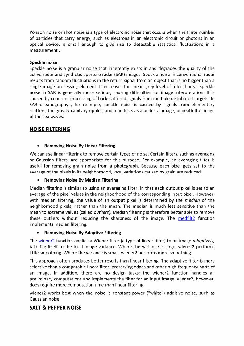
Poisson noise or shot noise is a type of electronic noise that occurs when the finite number of particles that carry energy, such as electrons in an electronic circuit or photons in an optical device, is small enough to give rise to detectable statistical fluctuations in a measurement . Speckle noise Speckle noise is a granular noise that inherently exists in and degrades the quality of the active radar and synthetic aperture radar (SAR) images. Speckle noise in conventional radar results from random fluctuations in the return signal from an object that is no bigger than a single image-processing element. It increases the mean grey level of a local area. Speckle noise in SAR is generally more serious, causing difficulties for image interpretation. It is caused by coherent processing of backscattered signals from multiple distributed targets. In SAR oceanography , for example, speckle noise is caused by signals from elementary scatters, the gravity-capillary ripples, and manifests as a pedestal image, beneath the image of the sea waves.

NOISE FILTERING

• Removing Noise By Linear Filtering

We can use linear filtering to remove certain types of noise. Certain filters, such as averaging or Gaussian filters, are appropriate for this purpose. For example, an averaging filter is useful for removing grain noise from a photograph. Because each pixel gets set to the average of the pixels in its neighborhood, local variations caused by grain are reduced.

• Removing Noise By Median Filtering

Median filtering is similar to using an averaging filter, in that each output pixel is set to an average of the pixel values in the neighborhood of the corresponding input pixel. However, with median filtering, the value of an output pixel is determined by the median of the neighborhood pixels, rather than the mean. The median is much less sensitive than the mean to extreme values (called outliers). Median filtering is therefore better able to remove these outliers without reducing the sharpness of the image. The medfilt2 function implements median filtering.

Removing Noise By Adaptive Filtering

The wiener2 function applies a Wiener filter (a type of linear filter) to an image adaptively, tailoring itself to the local image variance. Where the variance is large, wiener2 performs little smoothing. Where the variance is small, wiener2 performs more smoothing.

This approach often produces better results than linear filtering. The adaptive filter is more selective than a comparable linear filter, preserving edges and other high-frequency parts of an image. In addition, there are no design tasks; the wiener2 function handles all preliminary computations and implements the filter for an input image. wiener2, however, does require more computation time than linear filtering.

wiener2 works best when the noise is constant-power ("white") additive noise, such as Gaussian noise

SALT & PEPPER NOISE

Matlab Code-

f=imread('C:\Users\Jitesh\Desktop\tst.gif'); imshow(f),title('original image'); g=imnoise(f,'salt & pepper',0.05); figure,imshow(g),title('noisy image') h = fspecial('unsharp'); j=imfilter(g,h); figure,imshow(j),title(' linear filtered image') k = filter2(fspecial('average',3),g)/255; figure,imshow(k),title('FIR filtered image') l = medfilt2(g,[3 3]); figure,imshow(l),title(' median filtered image') m= wiener2(g,[5 5]); figure, imshow(m),title('adaptive filtered image')

GAUSSIAN NOISE

Matlab Code-

f=imread('C:\Users\Jitesh\Desktop\tst.gif'); imshow(f),title('original image'); g=imnoise(f,'gaussian',0,0.05); figure,imshow(g),title('noisy image') h = fspecial('unsharp'); j=imfilter(g,h); figure,imshow(j),title(' linear filtered image') k = filter2(fspecial('average',3),g)/255; figure,imshow(k),title('FIR filtered image') l = medfilt2(g,[3 3]); figure,imshow(l),title(' median filtered image') m= wiener2(g,[5 5]); figure, imshow(m),title('adaptive filtered image')

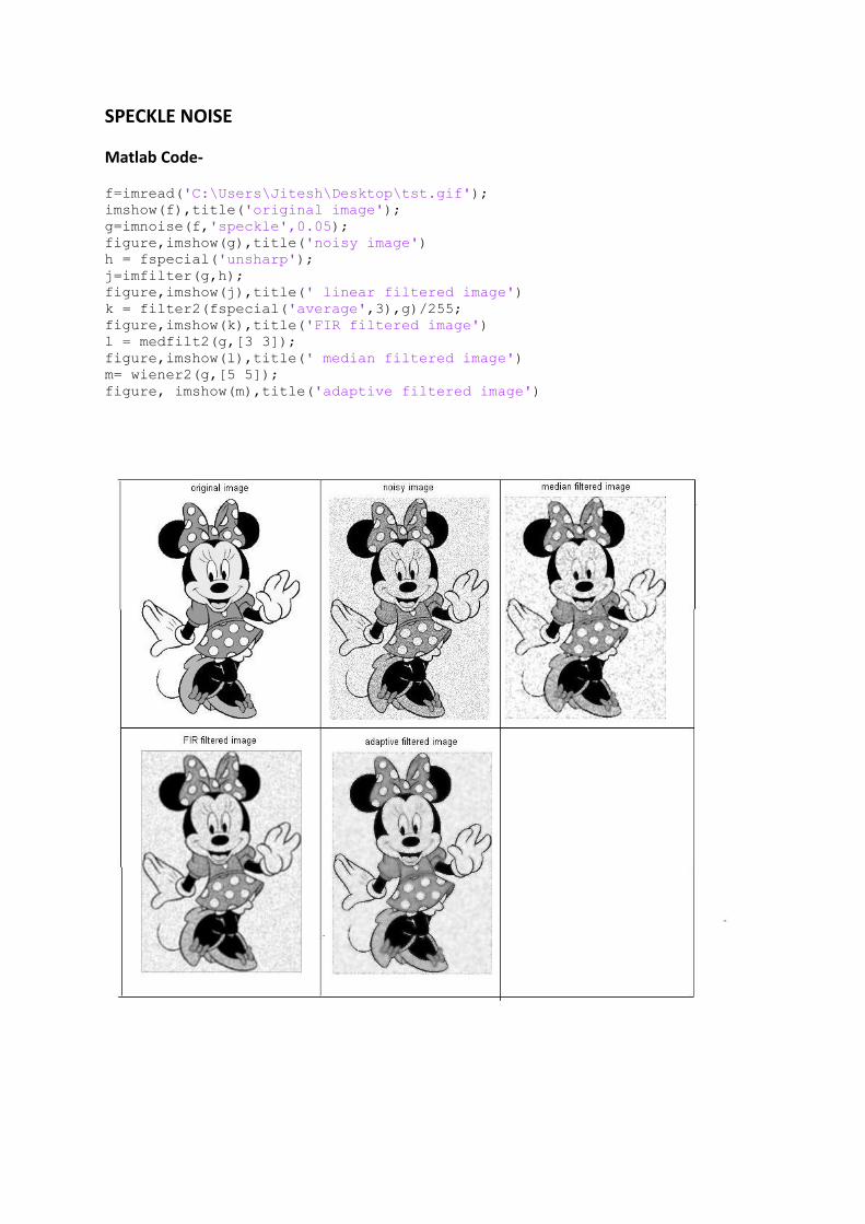
SPECKLE NOISE

Matlab Code-

f=imread('C:\Users\Jitesh\Desktop\tst.gif'); imshow(f),title('original image'); g=imnoise(f,'speckle',0.05); figure,imshow(g),title('noisy image') h = fspecial('unsharp'); j=imfilter(g,h); figure,imshow(j),title(' linear filtered image') k = filter2(fspecial('average',3),g)/255; figure,imshow(k),title('FIR filtered image') l = medfilt2(g,[3 3]); figure,imshow(l),title(' median filtered image') m= wiener2(g,[5 5]); figure, imshow(m),title('adaptive filtered image')

CONCLUSION

We used the Mini mouse Image in “gif” format ,adding four noise (Speckle, Gaussian ,Poisson and Salt & Pepper) in original image with standard deviation(0.025),De-noised all noisy images by all filters and conclude from the results that: (a)The performance of the Wiener Filter after de-noising for all Speckle, Poisson and Gaussian noise is better than Mean filter and Median filter. (b)The performance of the Median filter after de-noising for all Salt & Pepper noise is better than Mean filter and Wiener filter.

SCOPE FOR FUTURE WORK There are a couple of areas which we would like to improve on. One area is in improving the de-noising along the edges as the method we used did not perform so well along the edges. Another area of improvement would be to develop a better optimality criterion as the MSE is not always the best optimality criterion. The future work of research would be to implement Wiener Filter in Wavelet Domain, applying the methods in which the noise variance is known & in which the noise variance is unknown i.e. the MAD method.