1/33

�

�

�

�

�

�

College of the Redwoodshttp://online.redwoods.cc.ca.us/instruct/darnold/laproj/fall2002/ames/

Image Compression Using theHaar Wavelet Transform

Greg AmesCollege of the RedwoodsMath 45 Linear AlgebraInstructor - David Arnoldemail: freesoup@hotmail.com

2/33

�

�

�

�

�

�

Purpose

Digital images require large amounts of memory to store and, when

retrieved from the internet, can take a considerable amount of time to

download. The Haar wavelet transform provides a method of compress-

ing image data so that it takes up less memory. Today I will discuss the

implementation of the Haar wavelet transform and some of its applica-

tions.

3/33

�

�

�

�

�

�

Background

The files that comprise these images can be quite large and can quickly

take up precious memory space on the computer’s hard drive. A gray

scale image that is 256 x 256 pixels has 65, 536 elements to store, and a

typical 640 x 480 color image has nearly a million! The size of these files

can also make downloading from the internet a lengthy process. The

Haar wavelet transform provides a means by which we can compress

the image so that it takes up much less storage space, and therefore

transmits faster electronically and in progressive levels of detail.

4/33

�

�

�

�

�

�

How Images are Stored

Before we can understand how to manipulate an image, it is important

to understand exactly how the computer stores the image. A 256 x 256

pixel gray scale image is stored as a 256 x 256 matrix, with each element

of the matrix being a number ranging from zero (for black) to some

positive whole number (for white). A 256 x 256 color image is stored

as three 256 x 256 matrices (One each for the colors red, green, and

blue). We can use this matrix, and some linear algebra to maximize

compression while maintaining a suitable level of detail.

5/33

�

�

�

�

�

�

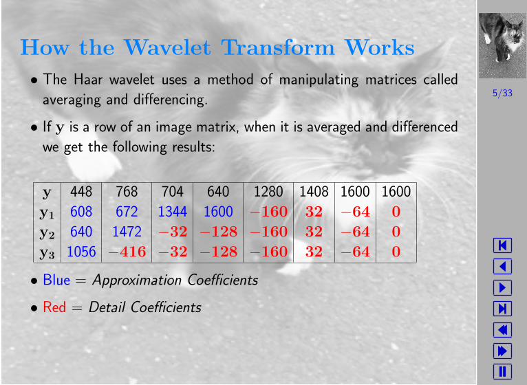
How the Wavelet Transform Works

• The Haar wavelet uses a method of manipulating matrices called

averaging and differencing.

• If y is a row of an image matrix, when it is averaged and differenced

we get the following results:

y 448 768 704 640 1280 1408 1600 1600

y1 608 672 1344 1600 −160 32 −64 0

y2 640 1472 −32 −128 −160 32 −64 0

y3 1056 −416 −32 −128 −160 32 −64 0

• Blue = Approximation Coefficients

• Red = Detail Coefficients

6/33

�

�

�

�

�

�

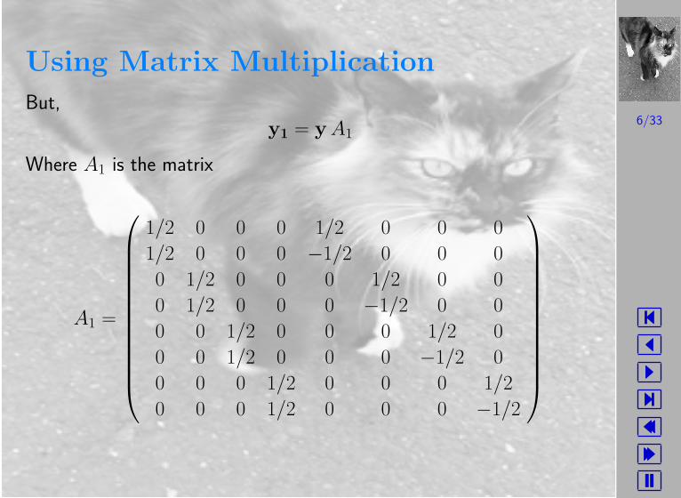
Using Matrix Multiplication

But,

y1 = y A1

Where A1 is the matrix

A1 =

1/2 0 0 0 1/2 0 0 0

1/2 0 0 0 −1/2 0 0 0

0 1/2 0 0 0 1/2 0 0

0 1/2 0 0 0 −1/2 0 0

0 0 1/2 0 0 0 1/2 0

0 0 1/2 0 0 0 −1/2 0

0 0 0 1/2 0 0 0 1/2

0 0 0 1/2 0 0 0 −1/2

7/33

�

�

�

�

�

�

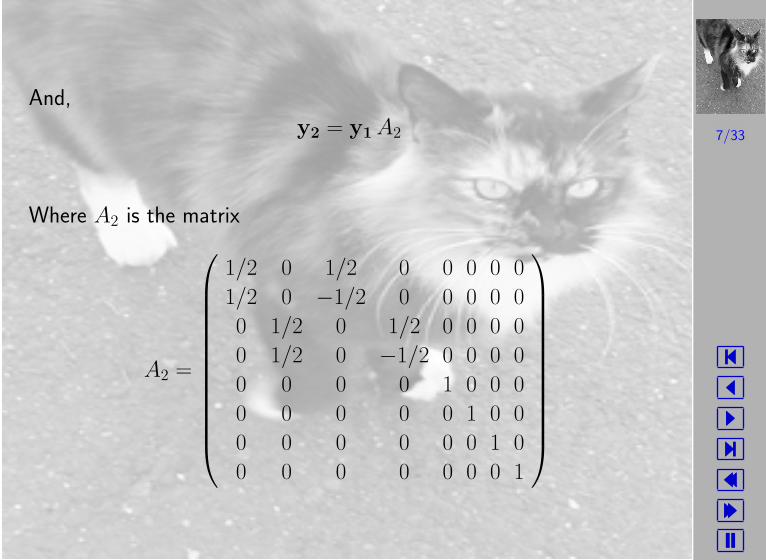
And,

y2 = y1 A2

Where A2 is the matrix

A2 =

1/2 0 1/2 0 0 0 0 0

1/2 0 −1/2 0 0 0 0 0

0 1/2 0 1/2 0 0 0 0

0 1/2 0 −1/2 0 0 0 0

0 0 0 0 1 0 0 0

0 0 0 0 0 1 0 0

0 0 0 0 0 0 1 0

0 0 0 0 0 0 0 1

8/33

�

�

�

�

�

�

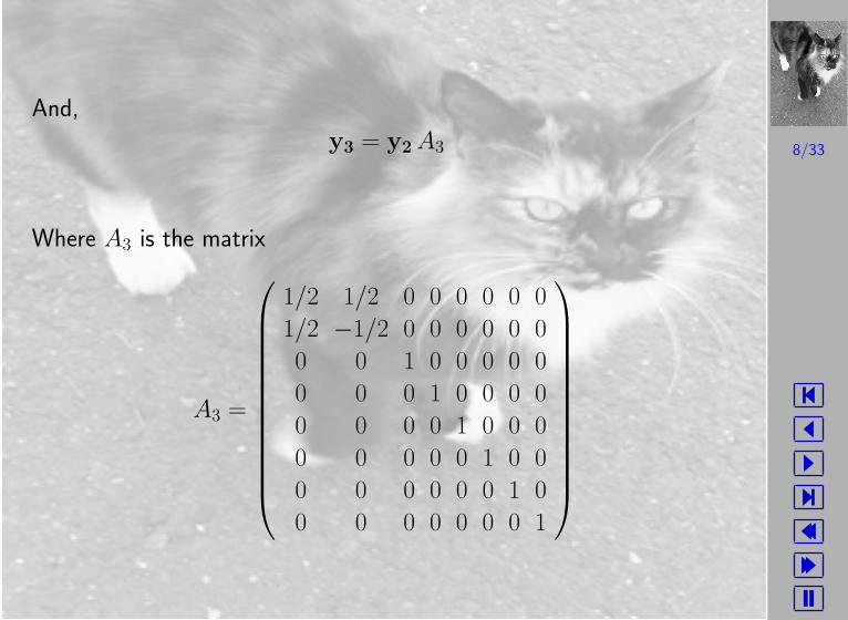
And,

y3 = y2 A3

Where A3 is the matrix

A3 =

1/2 1/2 0 0 0 0 0 0

1/2 −1/2 0 0 0 0 0 0

0 0 1 0 0 0 0 0

0 0 0 1 0 0 0 0

0 0 0 0 1 0 0 0

0 0 0 0 0 1 0 0

0 0 0 0 0 0 1 0

0 0 0 0 0 0 0 1

9/33

�

�

�

�

�

�

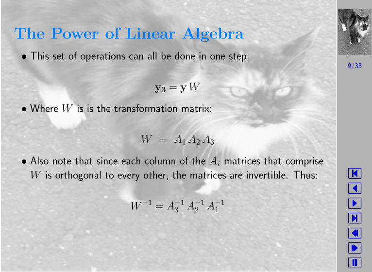
The Power of Linear Algebra

• This set of operations can all be done in one step:

y3 = y W

• Where W is is the transformation matrix:

W = A1 A2 A3

• Also note that since each column of the Ai matrices that comprise

W is orthogonal to every other, the matrices are invertible. Thus:

W−1 = A−13 A−1

2 A−11

10/33

�

�

�

�

�

�

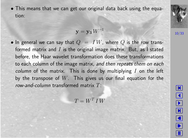
• This means that we can get our original data back using the equa-

tion:

y = y3 W−1

• In general we can say that Q = I W , where Q is the row trans-

formed matrix and I is the original image matrix. But, as I stated

before, the Haar wavelet transformation does these transformations

to each column of the image matrix, and then repeats them on each

column of the matrix. This is done by multiplying I on the left

by the transpose of W . This gives us our final equation for the

row-and-column transformed matrix T :

T = W T I W

11/33

�

�

�

�

�

�

• It also follows from this that we can get back to our original image

matrix I using the following equation:

I = (W T )−1 T W−1

12/33

�

�

�

�

�

�

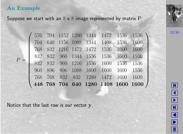
An Example

Suppose we start with an 8 x 8 image represented by matrix P:

P =

576 704 1152 1280 1344 1472 1536 1536

704 640 1156 1088 1344 1408 1536 1600

768 832 1216 1472 1472 1536 1600 1600

832 832 960 1344 1536 1536 1600 1536

832 832 960 1216 1536 1600 1536 1536

960 896 896 1088 1600 1600 1600 1536

768 768 832 832 1280 1472 1600 1600

448 768 704 640 1280 1408 1600 1600

Notice that the last row is our vector y.

13/33

�

�

�

�

�

�

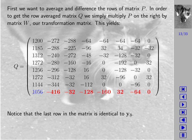
First we want to average and difference the rows of matrix P . In order

to get the row averaged matrix Q we simply multiply P on the right by

matrix W , our transformation matrix. This yields:

Q =

1200 −272 −288 −64 −64 −64 −64 0

1185 −288 −225 −96 32 34 −32 −32

1312 −240 −272 −48 −32 −128 −32 0

1272 −280 −160 −16 0 −192 0 32

1256 −296 −128 16 0 −128 −32 0

1272 −312 −32 16 32 −96 0 32

1144 −344 −32 −112 0 0 −96 0

1056 −416 −32 −128 −160 32 −64 0

Notice that the last row in the matrix is identical to y3.

14/33

�

�

�

�

�

�

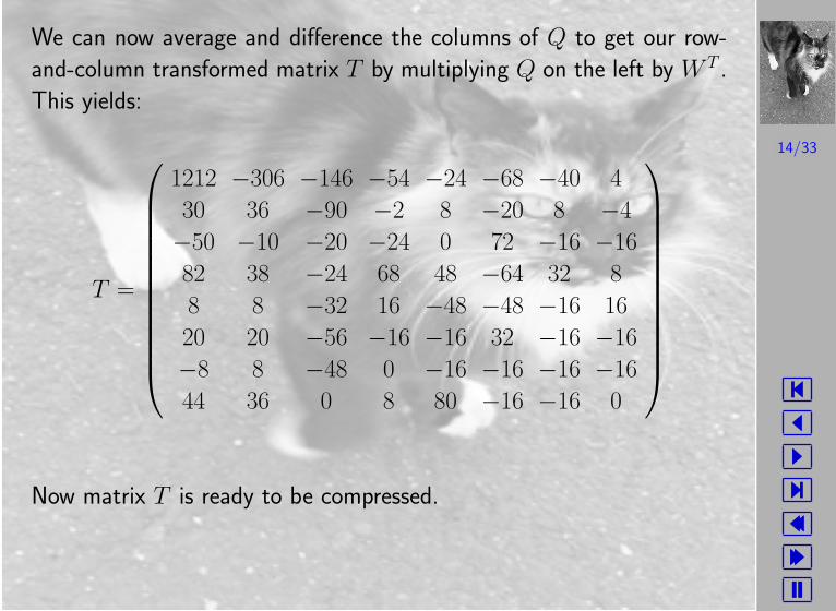
We can now average and difference the columns of Q to get our row-

and-column transformed matrix T by multiplying Q on the left by W T .

This yields:

T =

1212 −306 −146 −54 −24 −68 −40 4

30 36 −90 −2 8 −20 8 −4

−50 −10 −20 −24 0 72 −16 −16

82 38 −24 68 48 −64 32 8

8 8 −32 16 −48 −48 −16 16

20 20 −56 −16 −16 32 −16 −16

−8 8 −48 0 −16 −16 −16 −16

44 36 0 8 80 −16 −16 0

Now matrix T is ready to be compressed.

15/33

�

�

�

�

�

�

Even More Power

Another way to make these transformation matrices more powerful is to

normalize our transformation matrix W by dividing each column of W

by its length. The result is that W is orthogonal, meaning that each

column of the matrix is length one, and orthogonal to each other column

of the matrix. This is called a normalized wavelet transform. Having an

orthogonal transformation matrix has two major benefits:

1. First, because the inverse of an orthogonal matrix is equal to its

transpose, this greatly increases the speed at which we can perform

the calculations that reconstitute our image matrix.

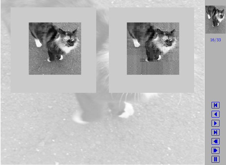
2. Second, as you can see from the following figure (compressed to

5.5 : 1), normalized transformations tend be closer to the original

image.

16/33

�

�

�

�

�

�

17/33

�

�

�

�

�

�

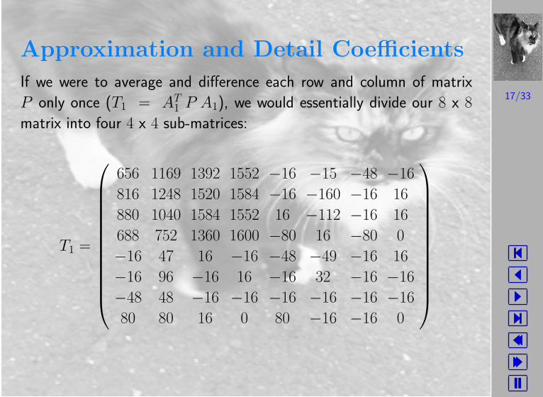
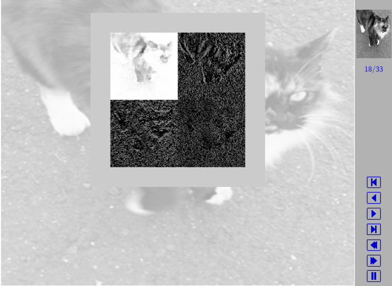
Approximation and Detail Coefficients

If we were to average and difference each row and column of matrix

P only once (T1 = AT1 P A1), we would essentially divide our 8 x 8

matrix into four 4 x 4 sub-matrices:

T1 =

656 1169 1392 1552 −16 −15 −48 −16

816 1248 1520 1584 −16 −160 −16 16

880 1040 1584 1552 16 −112 −16 16

688 752 1360 1600 −80 16 −80 0

−16 47 16 −16 −48 −49 −16 16

−16 96 −16 16 −16 32 −16 −16

−48 48 −16 −16 −16 −16 −16 −16

80 80 16 0 80 −16 −16 0

18/33

�

�

�

�

�

�

19/33

�

�

�

�

�

�

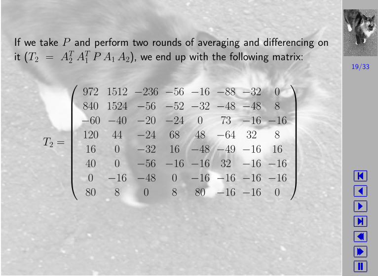
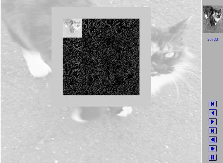
If we take P and perform two rounds of averaging and differencing on

it (T2 = AT2 AT

1 P A1 A2), we end up with the following matrix:

T2 =

972 1512 −236 −56 −16 −88 −32 0

840 1524 −56 −52 −32 −48 −48 8

−60 −40 −20 −24 0 73 −16 −16

120 44 −24 68 48 −64 32 8

16 0 −32 16 −48 −49 −16 16

40 0 −56 −16 −16 32 −16 −16

0 −16 −48 0 −16 −16 −16 −16

80 8 0 8 80 −16 −16 0

20/33

�

�

�

�

�

�

21/33

�

�

�

�

�

�

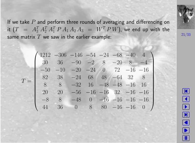
If we take P and perform three rounds of averaging and differencing on

it (T = AT3 AT

2 AT1 P A1 A2 A3 = W T P W ), we end up with the

same matrix T we saw in the earlier example:

T =

1212 −306 −146 −54 −24 −68 −40 4

30 36 −90 −2 8 −20 8 −4

−50 −10 −20 −24 0 72 −16 −16

82 38 −24 68 48 −64 32 8

8 8 −32 16 −48 −48 −16 16

20 20 −56 −16 −16 32 −16 −16

−8 8 −48 0 −16 −16 −16 −16

44 36 0 8 80 −16 −16 0

22/33

�

�

�

�

�

�

23/33

�

�

�

�

�

�

Wavelet CompressionImage compression using the Haar wavelet transform can be summed

up in a few simple steps.

1. Convert the image into a matrix format(I).

2. Calculate the row-and-column transformed matrix (T ) using T =

W T I W . The transformed matrix should be relatively sparse.

3. Select a threshold value ε, and replace any element of T less than ε

with a zero. This will result in a sparse matrix denoted as S.

4. To get our reconstructed matrix R from matrix S, we use an equa-

tion similar to I = (W T )−1 T W−1, but, because the inverse of an

orthogonal matrix is equal to its transpose, we modify the equation

as follows:

R = WSW−1

24/33

�

�

�

�

�

�

• If ε = 0, then S = T and therefore R = I . This is called

lossless compression.

• If ε > 0, then elements of T are reset to zero, and some original

data is lost. The reconstituted image will contain distortions. This

is called lossy compression.

• The secret of optimal compression is to choose ε so that compres-

sion is maximized while distortions in the reconstituted image are

minimized.

• The level of compression is measured by the compression ratio, which

is the ratio of nonzero entries in the transformed matrix T to the

number of nonzero entries in the compressed matrix S. According

to Dr. Colm Mulcahy of Spelman University, a compression ratio of

10 : 1 or greater means that S is sparse enough to have a significant

savings in terms of storage and transmission time.

25/33

�

�

�

�

�

�

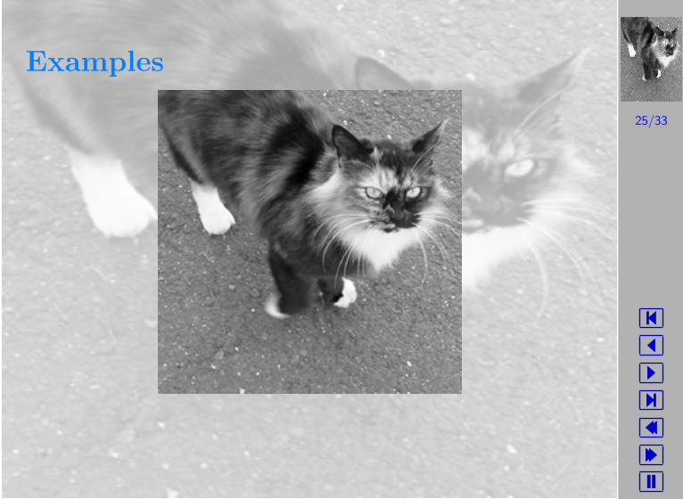
Examples

26/33

�

�

�

�

�

�

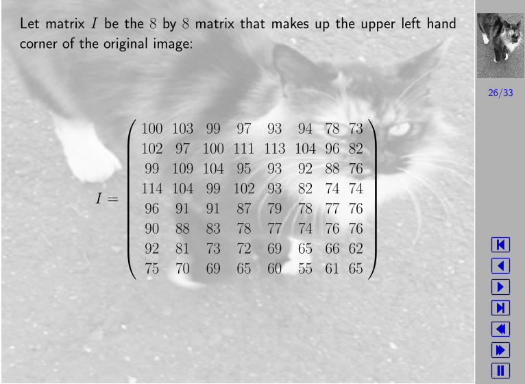
Let matrix I be the 8 by 8 matrix that makes up the upper left hand

corner of the original image:

I =

100 103 99 97 93 94 78 73

102 97 100 111 113 104 96 82

99 109 104 95 93 92 88 76

114 104 99 102 93 82 74 74

96 91 91 87 79 78 77 76

90 88 83 78 77 74 76 76

92 81 73 72 69 65 66 62

75 70 69 65 60 55 61 65

27/33

�

�

�

�

�

�

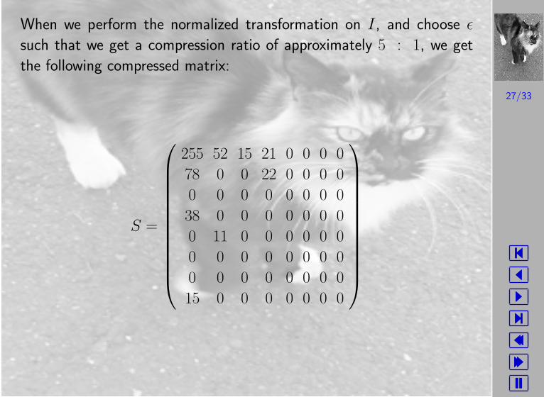
When we perform the normalized transformation on I , and choose ε

such that we get a compression ratio of approximately 5 : 1, we get

the following compressed matrix:

S =

255 52 15 21 0 0 0 0

78 0 0 22 0 0 0 0

0 0 0 0 0 0 0 0

38 0 0 0 0 0 0 0

0 11 0 0 0 0 0 0

0 0 0 0 0 0 0 0

0 0 0 0 0 0 0 0

15 0 0 0 0 0 0 0

28/33

�

�

�

�

�

�

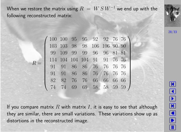
When we restore the matrix using R = W S W−1 we end up with the

following reconstructed matrix:

R =

100 100 95 95 92 92 76 76

103 103 98 98 106 106 90 90

99 109 99 99 96 96 81 81

114 104 104 104 91 91 76 76

91 91 86 86 76 76 76 76

91 91 86 86 76 76 76 76

82 82 76 76 66 66 66 66

74 74 69 69 58 58 59 59

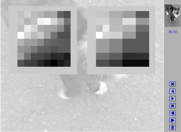
If you compare matrix R with matrix I , it is easy to see that although

they are similar, there are small variations. These variations show up as

distortions in the reconstructed image.

29/33

�

�

�

�

�

�

30/33

�

�

�

�

�

�

Electronic Transmission

People frequently download images from the internet, a few of which

are not even pornographic. Wavelet transforms enhance electronic trans-

fers of images in two ways:

• Because a compressed image file is significantly smaller it takes far

less time to download.

• Progressive Transmission - When an image is requested, the source

computer first sends the overall approximation coefficient and larger

detail coefficients, and then the progressively smaller detail coef-

ficients. As your computer receives this information it begins to

reconstruct the image in progressively greater detail until the origi-

nal image is fully reconstructed. This process can be interrupted at

any time. Otherwise an user would only be able to see an image

after the entire image file had been downloaded.

31/33

�

�

�

�

�

�

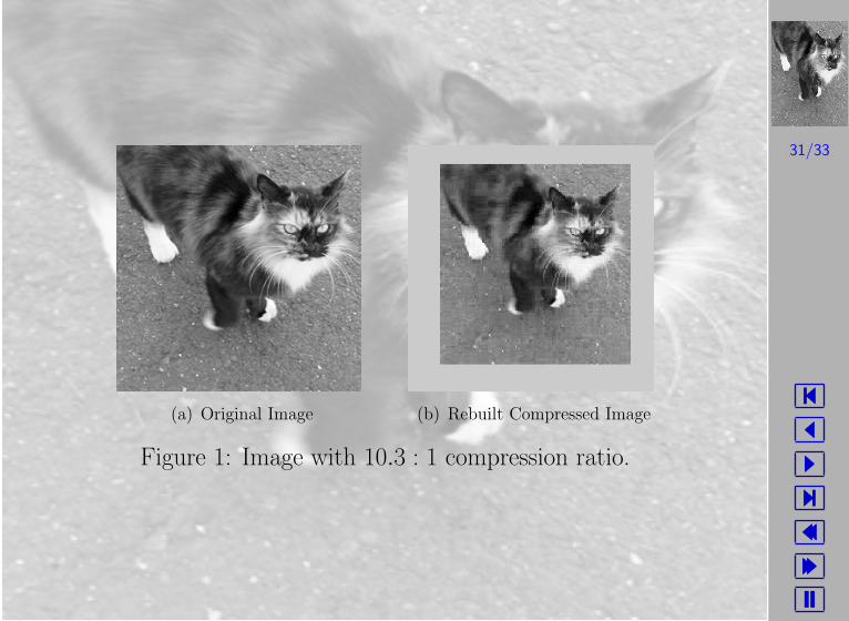
(a) Original Image (b) Rebuilt Compressed Image

Figure 1: Image with 10.3 : 1 compression ratio.

32/33

�

�

�

�

�

�

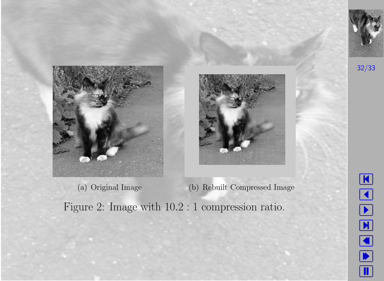
(a) Original Image (b) Rebuilt Compressed Image

Figure 2: Image with 10.2 : 1 compression ratio.

33/33

�

�

�

�

�

�

References

[1] Ames, Rebecca For instruction in Adobe Photoshop

[2] Arnold, Dave College of the Redwoods

[3] Huang, LiHong For his help in constructing the Matlab M-Files

[4] Mulcahy, Colm Image Compression Using the Haar Wavelet Trans-

form

[5] Strang, Gilbert Introduction to Linear Algebra