Image Compression Using BinDCT For Dynamic Hardware FPGA’s · 2008-02-13 · Image Compression...
208
Image Compression Using BinDCT For Dynamic Hardware FPGA’s Mahmoud Fawaz Khalil Al-Gherify A thesis submitted in partial fulfilment of the requirements of Liverpool John Moores University for the degree of Doctor of Philosophy General Engineering Research Institute (GERI), Liverpool John Moores University. May 2007
Transcript of Image Compression Using BinDCT For Dynamic Hardware FPGA’s · 2008-02-13 · Image Compression...

Image Compression Using BinDCT For Dynamic Hardware FPGA’s
Mahmoud Fawaz Khalil Al-Gherify
A thesis submitted in partial fulfilment of the requirements of Liverpool John Moores
University for the degree of Doctor of Philosophy
General Engineering Research Institute (GERI), Liverpool John Moores University. May 2007

Abstract
ABSTRACT
____________________________________________________________ This thesis investigates the prospect of using a Binary Discrete Cosine Transform as an
integral component of an image compression system. The Discrete Cosine Transform
(DCT) algorithm is well known and commonly used for image compression. Various
compression techniques are actively being researched as they are attractive for many
industrial applications. The particular compression technique focused on was still image
compression using the DCT. The recent expansion of image compression algorithms
and multimedia based mobile, including many wireless communication applications,
handheld devices, digital cameras, videophones, and PDAs has furthered the need for
more efficient ways to compress both digital signals and images.
The objective of this research to find a generic model to be used for image compression
was met. This software model uses the BinDCT algorithm and also develops a detection
system that is accurate and efficient for implementation in hardware, particularly to run
in real-time. This model once loaded on to any dynamic hardware should update by
reconfiguring the FPGA automatically, during run time with different BinDCT
processors. Such a model will enhance our understanding of the dynamic BinDCT
processor in image compression.
Image analysis involves examination of the image data for a specific application. The
characteristic of an image decides the most efficient algorithm. Selection techniques
were designed centred on use of the entropy calculation for each 8 x 8 tile. However
many other techniques were analysed such as homogeneity. Selection of the most
efficient BinDCT algorithm for each tile was a challenge met by analysis of the entropy
data. For the BinDCT different configurations were analysed with standard grey scale
photographic images.
Upgrading the available technology to the point where the most suitable BinDCT
configuration for each image tile input stream will be continuously configured all the
time, will lead to significant coding advantage in image analysis and traditional
i

Abstract
compression process. Hence, great performance can be achieved if the FPGA can
dynamically switch between the different configurations of the BinDCT transform.
ii

Acknowledgement
ACKNOWLEDGEMENT
____________________________________________________________
I am deeply indebted to my advisor team, Professor Dave Harvey, Doctor Ciaron
Murphy, Professor Dave Burton for their constant support. Without their help, this work
would not be possible. I would also like to thank all GERI group for the lovely work
environment they provided and whom always been their when I needed them.
I would like to thank all my friends for the outstanding advice throughout the years.
Special thanks to my best friends and colleagues in GERI Salah and Hussein for the
good time I spent with them and for the help they provided. I am also indebted to IMG
technologies LTD who give me the time and space when I needed it.
Lastly, I would like to thank my family for their support. I am greatly indebted to my
brother Ali who always pushed me further to finish this work efficiently. Above all, I
would like to express my deepest gratitude for the constant support, understanding and
love that I received from my parents, brothers and sisters.
I dedicate this thesis to my mother Amnah and father Fawaz.
iii

List of Figures
LIST OF FIGURES
____________________________________________________________
Chapter 2 Fig. 2.1 Chen Version of The Fast DCT [33]
Fig. 2.2: (a) Scaled Steps (b) General Butterfly
Fig. 2.3 (a) Lifting Structure (b) Scaled Lifting Structure
Fig. 2.4 Field Programmable Gate Array (FPGA) Internal Basic Structure
Fig. 2.5 Illustration of FPGA Based Architecture on Colour Processing Task
Chapter 3 Fig. 3.1 Basic Data Compression System
Fig. 3.2 Coordinate Rotation for Blocks of Two Sample (x, y) Domain and
(C1, C2) Domain.
Fig. 3.3 Output of The (8×8) 2-D DCT
Fig. 3.4 Common Lossless\ Lossy Signal Image Encoder Blocks
Fig. 3.5 Forward BinDCT [7]
Fig. 3.6 Inverse BinDCT [7]
Fig. 3.7 Ramp Function Input Stream
Fig. 3.8 Constant Function Input Stream
Fig. 3.9 Mexican Hat Function Input Stream
Fig. 3.10 Step Function Input Stream
Fig. 3.11 Spike Function Input Stream
Fig. 3.12 Ramp Function RMSE Values For Nine BinDCT Configurations
Fig. 3.13 Constant Function RMSE Values For Nine BinDCT Configurations
Fig. 3.14 Mexican Hat Function RMSE Values For Nine BinDCT Configurations
Fig. 3.15 Step Function RMSE Values For Nine BinDCT Configurations
Fig. 3.16 Spike Function RMSE Values For Nine BinDCT Configurations
Fig. 3.17 Lossless Compression Ratio For Nine Configurations And The Dynamic
BinDCT For Lena Image
Fig. 3.18 Lossless Zero Coefficients For Nine Configurations And The Dynamic
BinDCT For Lena Image.
iv

List of Figures
Fig. 3.19 Lossless RMSE Values For Nine Configurations And The Dynamic
BinDCT For Lena Image.
Fig. 3.20 Lossy Compression Ratio For Nine Configurations And The Dynamic
BinDCT For Lena Image
Fig. 3.21 Lossy RMSE Values For Nine Configurations And The Dynamic BinDCT
For Lena Image
Chapter 4 Fig. 4.1 The Flow Graph of The Entropy Operation
Fig. 4.2 Entropy Average For 20 Images
Fig. 4.3 Comparison Between The Two Average Sets
Fig. 4.4 Differences Between The Entropy Values And The Average For the Same
Points
Fig. 4.5 Forward Data Flow Diagram Processing Using Entropy Pre-processing
Stage
Fig. 4.6 Inverse Data Flow Diagram Processing Using Pre-processing Stage
Fig. 4.7 Forward Data Flow Diagram Processing Using Homogeneity Pre-
processing Stage
Fig. 4.8 Homogeneity Average For 20 Tested Images
Fig. 4.9 The New Calculated Average When Average Between Neighboured Points
Fig. 4.10 Reconstructed Lena Image Processed With Entropy Selection Technique
Fig. 4.11 Reconstructed Lena Image Processed With BinDCT-C1
Fig. 4.12 Reconstructed Lena Image Processed With BinDCT-C9
Fig. 4.13 Reconstructed Lena Image Processed With Entropy Selection Technique
Fig. 4.14 Reconstructed Tile Image Processed With Entropy Selection Technique
Fig. 4.15 Reconstructed Lena Not Quantized Image Processed With Homogeneity
Selection Technique
Fig. 4.16 Reconstructed Lena Quantized Image Processed With Homogeneity
Selection Technique
Fig. 4.17 Reconstructed Vegi Image Processed With Homogeneity Selection
Technique
Fig. 4.18 Reconstructed Vegi Image Processed With BinDCT -C1
Fig. 4.19 Reconstructed Lena Image Processed With BinDCT-C9
Fig. 4.20 Reconstructed Tile Image Processed With Homogeneity Selection
v

List of Figures
Technique.
Chapter 5 Fig. 5.1 Selection Technique Test Bench Structure
Fig. 5.2 Selection Technique connected to Dynamic Forward BinDCT Structure
Fig. 5.3 Selection Technique Pipe Line Structure
Fig. 5.4 Save Incoming Tile Block Structure
Fig. 5.5 Binary Shift Operation
Fig. 5.6 Timing Simulation of Stage One
Fig. 5.7 Selection Technique GLCM Block Structure
Fig. 5.8 GLCM Internal Block Structure
Fig. 5.9 Simulation of Stage Two
Fig. 5.10 Selection Technique Normalised GLCM Block Structure
Fig. 5.11 Timing Simulation of Stage Three
Fig. 5.12 Selection Technique Log Function Block Structure
Fig. 5.13 Creating The Two Input Port From α
Fig. 5.14 Timing Simulation of Stage Four
Fig. 5.15 CORDIC IP Core With The Index Interface
Fig. 5.16 The Operational Procedures of The Multiplier Design
Fig. 5.17 Timing Simulations For Stage Five
Chapter 6 Fig. 6.1 Two Dimensional BinDCT Processor Blocks
Fig. 6.2 1D BinDCT Transform Function Implementation Stages
Fig. 6.3 Stage One Circuit Diagram
Fig. 6.4 A 15 Bits Registers
Fig. 6.5 BinDCT Stage Two Circuit Diagram
Fig. 6.6 Stage Four Circuit Diagram
Fig. 6.7 Stage Four Circuit Diagram
Fig. 6.8 Stage Five Circuit Diagram
Fig. 6.9 Static BinDCT Implementation
Fig. 6.10 Simulated Five Stages of The Two-Dimensional BinDCT
Fig. 6.11 Design FloorPlanner
Fig. 6.12 The Generic FBinDCT With Configuration Lookup Table
vi

List of Figures
Fig. 6.13 Genric FBinDCT Chip Interface Ports
Fig. 6.14 FBinDCT RTL Sub-Blocks Design
Fig. 6.15 Generic FBinDCT Design FloorPlanner
Fig. 6.16 Generic InvBinDCT Chip Interface Ports
Fig. 6.17 InvBinDCT RTL Sub-Blocks Design
Fig. 6.18 Generic InvBinDCT Design FloorPlanner
Fig. 6.19 Dynamic BinDCT Sub-Block Design
Fig. 6.20 Dynamic BinDCT Connected RTLdesign
Fig. 6.21 Timing Simulation For Lena During Forward Transformation Operation
Fig. 6.22 Timing Simulation For Lena During Inverse Transformation Operation
Fig. 6.23 Lena Tile Based Verification Result
Fig. 6.24 Reconstructed Lena Image Using VHDL Reconfigurable Design
Fig. 6.25 Timing Simulation For Tile Image during Forward Transformation
Operation
Fig. 6.26 Timing Simulation for Tile Image during Inverse Transformation
Operation
Fig. 6.27 Last Tile of Tile Image Verification Result
Fig. 6.28 Reconstructed Tile Image Using VHDL Reconfigurable Design
Chapter 7 Fig. 7.1 The Generic System Components.
Fig. 7.2 PC405 to Calculate The Selection Technique And FPGA to Calculate The
BinDCT Algorithm.
Fig. 7.3 Multi-FPGA System to Calculate The Combined Entropy Selection
Technique And The FBinDCT Processor
Fig. 7.4 Proposed Dynamic Loosy-Lossless Image Compression System
vii

List of Tables
LIST OF TABLES
____________________________________________________________
Chapter 2 Table 2.1 Popular FDCT Algorithms Computation When N=8
Chapter 3 Table 3.1 Different Dyadic Parameters Values For All BinDCT Configurations
Table 3.2 Forward BinDCT Scaling Factor Table 3.3 Reverse BinDCT Scaling
Factor
Table 3.4 RMSE Value Results From Processing The Five Functions Using All
BinDCT Configurations
Table 3.5 Input Streams With Most Suitable Algorithm
Table 3.6 Results of Lossless Compression on Lena Image.
Table 3.6 Quantization Matrix Used
Table 3.7 Quantized Lena Image For Loosy Image Compression
Chapter 4 Table 4.1 GLCM Operation
Table 4.2 GLCM Grey Level Combination
Table 4.3 GLCM Matrix
Table 4.5 Normalization Operation
Table 4.6 Entropy Values Results from Processing 20 Images For Nine BinDCT
Configurations
Table 4.8 Homogeneity Values Results from Processing 20 Images For Nine
BinDCT Configurations
Table 4.9 Software C Code Simulation Results When Entropy Pre-processing
Stage Operates on Lena Image
Table 4.10 Reconstruction RMSE for Lena ImageWwith Entropy Technique
Table 4.11 Software C Code Simulation Results When Entropy Pre-processing
Stage Operates On Tile Image
Table 4.12 Reconstruction RMSE For Tile Image with Entropy Technique
viii

List of Tables
Table 4.13 Software C Code Simulation Results When Homogeneity Pre-
processing Stage Operates on Lena Image
Table 4.14 Reconstruction RMSE Lena Image With Homogeneity Technique
Table 4.15 Software C Code Simulation Results When Homogeneity Pre-
processing Stage Operates on Vegi Image
Table 4.16 Reconstruction RMSE For Vegi Image with Homogeneity Technique
Table 4.17 Comparison Between Results of The Two Proposed Selection
Techniques
Chapter 5 Table 5.1 Stage One Interface Port Map
Table 5.2 Stage Two Interface Port Map
Table 5.3 The Calculation of the GLCM for STORE_IMAGE_PIXEL Grey Levels
(2, 2)
Table 5.4 The Whole GLCM Table For This Particular Tile
Table 5.5 Stage Three Interface Port Map
Table 5.6 Division Algorithm Working Example
Table 5.7 Stage Four Log Function Interface Port Map
Table 5.8 Input Data Representation
Table 5.9 Output Data Representation
Table 5.10 Stage Five Index Interface Port Map
Table 5.11 Fractional Portion of The Entropy Boundaries
Table 5.12 Entropy Boundaries For All Configurations
Chapter 6 Table 6.1 Stage One Interface Ports Operations
Table 6.2 Stage Two Interface Ports Operations
Table 6.3 Stage Three Port Interface Operations
Table 6.4 Stage Four Operations
Table 6.5 Stage Five Operations
Table 6.6 FPGA Resources Needed When Implementing Pipeline Static BinDCT
Using VHDL
Table 6.7 Distribution of The Components Inside Configurations C1 And C9.
ix

List of Tables
Table 6.8 Percentage of The Area Occupied From The FPGA For All
Configurations
Table 6.9 Hardware Resources For The Generic FBinDCT System
Table 6.10 Dynamic FBinDCT Design Macro Statistics
Table 6.11 Device Utilisation Summary Inv 2D BinDCT
Table 6.12 Dynamic InvBinDCT Design Macro Statistics
x

List of Abbreviations
LIST OF ABBREVIATIONS
____________________________________________________________ BinDCT Binary Discrete Cosine Transform
BinDCT-C1..C9 Binary Discrete Cosine Transform configuration 1 to 9
FBinDCT Forward Binary Discrete Cosine Transform
INVBINDCT Inverse Binary Discrete Cosine Transform
DCT Discrete Cosine Transfer
GLCM Gray Level Co-occurrences Matrix
RMSE Root Mean Square Error
ID Identity
C Software Programming Language
VHDL Vary high speed integrated circuit Hardware Description
Language
IP Intellectual Property
1D One Dimension
2D Two Dimension
FIFO First In First Out
DIN Data in
Xa0_Xa7 Input sample 0 to 7
CLK Clock signal
RST Reset signal
CNTR Counter signal
MSB Most Significant Bit
LSB Least Significant Bit
I/O Input or Output signal
FPGA Field Programmable Gate Array
MATLAB Matrix Laboratory (software environment)
IDL Interactive Data Language (software environment)
RAM Read And write Memory
ROM Read Only Memory
MHZ MegaHertz (Million hertz)
ns nano second
xi

List of Abbreviations
LUT Look Up Table
RTL Register Transfer Level
RTR Run Time Reconfigurable System
JTAG Joint Test Action Group
ASIC Application Specific Integrated Circuit
CORDIC Coordinate Rotation Digital Computer
Ceiling Truncation function in C
Floor Truncation function in C
Loc0 Location 0
IC Integrated Circuit
WL Word Length
Ln Natural logarithmic function
LOG Logarithmic function to base 2.
RDY Ready
Reg Register
PDA Personal Digital Assistant
ISO International Standards Organisation
IEC International Electro-Technical Commission
MPEG Moving Picture Experts Group
JPEG Joint Photographic Expert Group
DSP Digital Signal Processing
MP3 MPEG Audio Layer III
VLIW Very Long Instruction Word
TV Television
CCD Charge Couple Device
PC Personal Computer
VCR Videocassette Recorder
VPX Video Pixel Decoder
USB Universal Serial Bus
DC Direct Current
AC Alternative current
DA Distributed Arithmetic
SS Subexpression Sharing
CSD Canonic Signed Digit
xii
List of Abbreviations
IDCT Inverse Discrete Cosine Transform
FDCT Forward Discrete Cosine Transform
MMM Matrix-Matrix Multiplication
FFT Fast Fourier Transform
WHT Walsh-Hadamard Transform
PLD Programmable Logic Devices
HDL Hardware Description Language
CSW Context Switching
PRFPGAs Partially Reconfigurable Field Programmable Gate Arrays
RLE Run Length Encoding
Tiff Tagged Image File Format
RGB Red, Green, Blue
SNR Signal to Noise Ratio
PSNR Peak Signal to Noise Ratio
C DCT Coefficient R
ZIP Zoning Improvement Plan, file contains one or more files
that have been compressed
PNG Portable Network Graphics, a format designed for
transferring images on the Internet
GIF Graphics Interchange Format, an 8 bit per pixel bitmap
image format
Fig Figure GUI General User Interfeace
xiii

List of Symbols
LIST OF SYMBOLS
____________________________________________________________ P(E) Probability of event E
I(E) Unit or quantity of information
E Entropy
N1 Information carrying units in first data set
N2 Information carrying units in second set
V Vertical axes
H Horizontal axis
X(h,v) Sample in horizontal and vertical axes of the image under test
∞ Infinity value
E Energy for original spatial domain O
E Energy for new Frequency domain N
QI Integer part of the fix point number notation
QF Fractional part of the fix point number notation
xiv

List of Symbols
TABLE OF CONTENTS
____________________________________________________________
ABSTRAC ………………………………………………………………………. i ACKNOWLEDGEMENT …………………………………………………… Iii LIST OF FIGURES …………………………………………………………... iv LIST OF TABLES ……………………………………………………………. viii LIST OF ABBREVIATIONS ……………………………………………….. xi LIST OF SYMBOLS …………………………………………..……………… xiv TABLE OF CONTENTS…………………………………………………....... xv
1. INTRODUCTION…………………………………………………………. 1 1.1. Primary Remarks …………………………………………………… 1
1.2. Research Objectives …………………………………………….. 3
1.3. Research Methodology …………………………………………… 4
1.3.1 Problem Defined…………………………………………. 4
1.3.1.1 Hardware Implementations……………………… 4
1.3.1.2 Software Implantations………………………….. 4
1.3.2 Proposed Solution……………………………………….. 5
1.3.3 Development of Solution…………………………………. 6
1.3.4 Experimental Evaluation……………………………….. 6
1.4 Originality of The Research………………………………………. 6
1.5 Organisation of The Thesis……………………………………….. 8
2. LITETURE REVIEW …………………………………………………….. 10 2.1 Introduction………………………………………………………… 10
2.2 Review on The DCT Algorithms ………………………………… 11
2.2.1 DCT Back ground ………………………………………. 11
2.2.2 Fast DCT Algorithms …………………………………… 12
2.2.3 BinDCT Algorithms ……………………………………. 15
xv

List of Symbols
2.3 Review on The Architecture of The DCT ………………………. 18
2.3.1 Distributed Arithmetic (DA) ……………………………. 18
2.3.2 Canonical Signed Digit (CSD) ………………………… ….. 19
2.3.3 Subexpression Sharing (SS) ……………………………… 20
2.4 Review on The Implementation of The DCT/IDCT …………….. 20
2.4.1 DCT Hardware’s Platforms ………………………………. 20
2.5 FPGA Based Architectures ……………………………………… 23
2.5.1 Static FPGA Configuration……………………………….. 25
2.5.1.1 Serial Implementation…………………………….. 25
2.5.1.2 Parallel Implementation………………………….. 26
2.5.2 Dynamic FPGA Configuration ………………….. 27
2.5.3 Context Switching FPGA Configuration ………… 28
2.6 Summary ………………………………………………… 29
3. BINDCT TRANSFORM INTEGRATED PART OF IMAGE
COMPRESSION ………………………………………………………..
30
3.1 Introduction to Basic Principals of Image Compression…… 30
3.2 Inheritance Information Redundancy ……………………. 31
3.3 Types of Image Compression …………………………….. 33
3.4 Implementations of The Transformation Part …………….. 33
3.5 Reconfigurable BinDCT Transform Approach …………… 37
3.5.1 Preliminary Investigations …………………….. 38
3.5.2 Lossless Compression ……………………………. 48
3.5.3 Lossy Compression ……………………………….. 52
3.6 Implementations of Lossless Compression ………………. 55
3.7 Implementations of Lossy Compression ………………….. 56
3.8 Summary …………………………………………………. 56
4. MODELLING AND SELECTION TECHNIQUES ALGORTHIMS.. 59
4.1 Introduction…………………………………………………….. 59
4.2 Methods to Exploit Information From The Source Image…….… 60
4.2.1 Elements of Information Theory ………………………… 60
4.2.2 Gray Level Co-occurrence Matrix (GLCM) …………… 60
xvi

List of Symbols
4.2.2.1 Construction of The GLCM …………………. 61
4.2.3 Normalisation …………………………………………. 64
4.2.4 Entropy ……………………………………………….. 65
4.2.5 Homogeneity …………………………………………… 65
4.3 Entropy Operational Procedures …………………………….. 66
4.4 Experimental Work on Entropy Selection Technique………….. 78
4.4.1 Lena Image ……………………………………………… 78
4.4.2 Repeated Constant Tiles Image ………………………….. 82
4.5 Experimental Work on Homogeneity Selection Technique ……. 84
4.5.1 Lena Image ……………………………………………….. 84
4.5.2 Vegi Image ………………………………………………. 86
4.5.3 Repeated Constant Tiles ………………………………… 89
4.6 Summary ………………………………………………………… 89
5 . ENTROPY SELECTION HARDWARE DESIGN ………………… 91 5.1 Introduction ………………………………………………………. 91
5.2 VHDL Features …………………………………………………. 91
5.2.1 VHDL as a Simulation Modelling Tool ………………. 92
5.2.2 VHDL as Design Entry Tool ………………………….. 92
5.2.3 VHDL as Netlist Generator Tool …………………….. 92
5.2.4 VHDL as Verification Tool …………………………… 92
5.3 Selection Technique Sub-Blocks ………………………………… 93
5.3.1 Storing The Incoming Tile Stage ………………………. 96
5.3.2 Functional Description ………………………………… 97
5.3.3 Timing Simulation……………………………………….. 98
5.4 GLCM Calculator Design Stage …………………………………. 99
5.4.1 Functional Description……………………………………… 100
5.4.2 Timing Simulation Test…………………………………….. 102
5.5 Normalising The GLCM Stage ……………………………………. 105
5.5.1 Functional Description ……………………………………. 106
5.5.1.1 Division Algorithm …………………………….. 107
5.5.2 Timing Simulation Test ………………………………….. 111
5.6 Log function And Index Design…………………………………… 112
xvii

List of Symbols
5.6.1 Functional Description ………………………………….. 113
5.6.1.1 Input Port Calculations………………………… 114
5.6.1.2 Output Port Calculation ………………………… 116
5.6.2 Timing Simulation Test ……………………………………. 116
5.7 Index Design ……………………………………………………… 119
5.7.1 Functional Description …………………………………….. 120
5.7.2 Multiplication Algorithm ………………………………….. 121
5.7.3 Timing Simulation Test…………………………………… 124
5.8 Summary ………………………………………………………… 124
6. DYNAMIC BINDCT HARDWARE DESIGN ……………………….. 126 6.1 Introduction………………………………….……………………… 126
6.2 BinDCT Architecture Design ………………………………….. 127
6.3 1D BinDCT Stages Design ……………………………………. 130
6.3.1 Stage One ……………………………………………… 130
6.3.2 Stage Two ……………………………………………… 132
6.3.3 Stage Three …………………………………………….. 136
6.3.4 Stage Four of The BinDCT Data Flow Design ………. .. 137
6.3.5 Stage Five ……………………………………………… 138
6.3.6 Memory Block ………………………………………….. 140
6.3.7 2D BinDCT ……………………………………………… 140
6.3.8 InvBinDCT ……………………………………………. 141
6.4 Static BinDCT System Implementation ……………………….. 141
6.4.1 VHDL BinDCT Processor Experimental work ……….. 142
6.5 The New Dynamic Forward BinDCT Algorithm ………………. 146
6.6 Dynamic BinDCT System Implementation ……………………. 147
6.6.1 Generic 2D FBinDCT ………………………………….. 147
6.6.2 Generic 2D InvBinDCT…………………………………. 150
6.7 Selection module synthesis results ……………………………… 156
6.8 Verification And Implementation Results………………………. 157
6.8.1 Lena Image ……………………………………………… 157
6 .8.2 Tiles Image ……… …………………………………….. 160
6.8. 3 FPGA Hardware Implementation……………………….. 162
xviii

List of Symbols
6.9 Summary …………………………………………………………. 162
7. RECOMMENDATIONS FOR FUTURE WORK AND CONCLUSIONS 164 7.1 Introduction ……………………………………………………… 164
7.2 Hardware Implementation ………………………………………. 164
7.2.1 System Overview ………………………………………… 165
7.2.2 Power Processor-FPGA System Development Board to
Implement The Suggested Coupled Dynamic BinDCT
System…………………………………………………..
167
7.2.3 Multi-FPGA System Development Board ……………. 168
7.3 Software Implementation…………………………………………. 169
7.4 Proposing New System ……………………………………….. 170
7.5 Conclusion …………………………………………………………. 171
Appendix ………………………………………………………………………. 172
References……………………………………………………………………… 181
xix

1. INTRODUCTION
Chapter 1
INTRODUCTION
____________________________________________________________ 1. Primary Remarks The recent expansion of image compression algorithms and multimedia based mobile
and web applications, associated with the emerging new technologies has increased the
needs for more efficient ways to compress digital signals and images. The needs for
developing more powerful processor architectures to satisfy this requirement push
further for application diversity. Many wireless communication applications such as
handheld devices, digital cameras, videophones, multimedia mobiles, and the Personal
Digital Assistant PDAs suffer from both limited memory capacity and power resources.
The best implementations of image compression and decompression for these devices
therefore would be the one having maximum throughputs with minimum power
consumption.
An image is a two dimensional array of numbers. Each number corresponds to one
small area of the visual image, and the number gives the level of darkness or lightness
of that area. Each small area to which a number is assigned is called pixel. The size of
the physical area represented by a pixel is called the spatial resolution of the pixel. The
minimum value a pixel can have is typically 0 and the maximum value depends on how
the number is stored in the computer. The most common way is to store the pixel as a
byte, in which the pixel maximum value is 255. In byte format, pixels’ values can only
be integers. There are many image compression standards which exist, such as the still-
image compression standard JPEG ‘Joint Photo graphics Experts Group’ [1], a standard
established in 1992 by ISO (International Standards Organisation), IEC (International
Electro-Technical Commission), H.261 and H.263 videoconferencing standards and
MPEG-1, MPEG-2 and MPEG-4 digital video standards. Digital image compression
applications are common today. They can be found in our daily life from simple to very
complicated systems, such as the analogue and digital TV, computers, Internet,
multimedia mobile phones, MP3 players, and machine vision systems.
1

1. INTRODUCTION
The data collected from the sensors of all digital devices must first undergo a
mathematical transformation to perform data compression. Since it invented in 1974[2]
DCT has been successfully applied to the coding of high resolution [3 – 5]. It can be
regarded as a discrete time version of the Fourier Cosine series, a technique for
converting a signal into elementary frequency components. DCT implemented in a
single integrated circuit packing the most information into the fewest coefficients.
Because DCT require highly, complex computational and intensive calculations, a more
efficient algorithm to simplify and reduce number of arithmetic operation are needed.
Fast Discrete Cosine Transform (FDCT) consisting of alternating cosine/sine butterfly
matrices to reorder the matrix elements to a form which preserves a recognizable bit
reversed pattern at every node is set by Chen paper in 1977 [6].
All proposed FDCT algorithms produce or require floating point multiplications and
addition units. Floating point computation requires either large process die areas, or
slow software emulation which consider less efficient and not compatible to use with
the wireless and limited power devices. To achieve faster implementation the floating
point can be replace by fixed point, with cost of introducing results with rounding error.
Reports show that speed –up gained when implementing direct fixed-point execution
compared to emulating floating point varies between 20 for traditional DSP
architectures and 400 for deeply pipelined VLIW architectures. As well as fixed point
numbers require fewer bits than floating point numbers [7]. Designing Fast-DCT that
can be implemented with narrower bus width and simpler arithmetic operations, such as
shift and addition, remain a very rich research topic.
BinDCT one of the newest published Fast-DCT by Trans and Liang .The proposed new
algorithm that suited the fixed point multiplications with narrower data buses’ widths by
using a multiplier-less approximation of Chen’s Fast-DCT. They replaced all plane
rotations by a series of hardware friendly integer dyadic lifting-steps value. Since the
lifting values vary in there accuracy they proposed nine dyadic lifting configurations
BinDCT1 to BinDCT9 with varying degree of complexity to approximate the true
DCT[8]. The best use of the nine Binary Discrete Cosine Transform as an integral
component of any image compression system will be investigated in this research.
2

1. INTRODUCTION
1.2 Research Objectives Research novelty and objectives undertaken in this project are highlighted in this
section as follows:
1- Investigate, design, simulate and develop a novel selection control system for the
image compression transformation stage to improve the throughput and reduce the
timing.
2- Investigate, design and develop a dynamic reconfigurable BinDCT system to be
used with the FPGA environment to dynamically switch between different BinDCT
configurations during run-time forward and inverse transformation of the image.The
need for such model is very important for the following reasons:
1-Until now no satisfactory generic model other than the proposed work within
this thesis can automatically run to optimise for all BinDCT configurations,
with the ability to detect the best configuration for each incoming row tile of
the image in real time.
2- A number of advantages gained from this model will be:
• This model will yield to great savings in transmission time, and storage
capacity during both encoding and decoding the signal.
• Increase in compression ratio and coding gain.
• Real-time image compression.
• This model can be used for simulation purposes as part of other larger
designs.
3

1. INTRODUCTION
1.3 Research Methodology To understand the research novelty and objectives presented in the previous section, the
researches work is executed and formed according to the following subjects:
1.3.1 Problem Definition
On the basis of a relevant literature review, comprehensive study that cover the DCT
and BinDCT algorithms in terms of mathematical derivations and hardware
implementations, image compression techniques suffer from both hardware and
software implementations.
1.3.1.1 Hardware Implementations
The persist demand for data storage capacity and data transmission bandwidth continues
to exceed the rapid progress made in producing mass-storage density, processor speeds,
and greater digital communication system performance. The recent growth of image
compression algorithms and data intensive multimedia based web applications have not
only sustained the need for more efficient ways to encode signals and images but have
made compression of such signal central to storage and communication technology.
The problem investigated in this research is based on the fact that current image
compression techniques mainly depend on dedicated and rigid silicon hardware. This
causes inflexibility when implementing the DCT algorithms using both Digital Signal
Processors (DSPs) and Application Specific Integrated Circuits (ASICs). System
engineers face limitations because these devices are not flexible enough to continue to
follow the changes with new generations of the image compression algorithms.
1.3.1.2 Software Implantations
Most of the international image compression standard such JPEG, H.261 and H.263
software tools and hardware devices, uses only one transform algorithm to code the
complete image. If the BinDCT processor continues unchanging on the same
configuration, while the input image data stream frequency contents vary, coding gain
and throughput cannot be maximised as it will be discussed later in the next chapter.
4

1. INTRODUCTION
The software problem has been identified through the following questions:
a) How is it possible to improve the throughput, and which configuration give the most
efficient architecture?
b) How is it possible to combine use of more than one BinDCT algorithm to transform
the same image?
The first question defines the problem in the transform part of the compression system.
That will affect the processing time and storage space. This question takes into
consideration the knowledge in the image compression algorithms and falls under the
implementations of the image compression development methodology, while the second
question defines a general pre-processing control problem. It takes into consideration
the knowledge in the field of the image processing techniques.
1.3.2 Proposed Solution
The proposed solution for the first problem is to test each one of the nine BinDCT
configurations separately and compare the results between all of them in terms of
RMSE and the quality of the reconstructed image. The investigation is developed,
analysed and simulated with the aid of C, IDL, MATLAB and VHDL programming
languages.
The second proposed solution for the second problem is by developing and designing a
selection technique control system to switch between different configurations of the
BinDCT during run-time operation.
Upgrading the available technology to the point where the most suitable BinDCT
configuration for each image tile (8×8), or each 8-point input stream will be
continuously configured all the time, will lead to significant coding advantage and
processing speed up. Investigation done so far shows that great advantages in
performance can be achieved when dynamically switching between different
configurations of the BinDCT transforms is used.
5

1. INTRODUCTION
1.3.3 Development of Solution
The investigation carried out to appreciate the effect of use each BinDCT configuration
on reconstructing the image and on a tile based leads to believe that a model must
present to switch between different configurations. The novel arbitration like circuit
Entropy selection technique and Homogeneity selection technique developed
mathematically using texture analysis methods of the digital signal processing. The
mathematical relationship between different pixels of the same tile in terms of
frequency content variation was used to identify the best configuration to process each
tile. The proposed selection mechanism was coupled with the forward BinDCT
algorithm to form the dynamic reconfigurable BinDCT system.
1.3.4 Experimental evaluation
This proposed coupling system for both entropy and homogeneity was developed, tested
and analysed using C Language. the reconstructed images displayed with aid of IDL.
The entropy selection technique functional description coupled with the forward
BinDCT then developed in VHDL and the reconstructed images are also displayed with
IDL image processing software environment.
1.5 Originality of The Research The theory behind using the Binary Discrete Cosine Transform (BinDCT) in image
compression is discussed in detail in section 3.1.1. To meet the objectives of this
research initially we will investigate the existing dynamically switching between
BinDCT type 1 and type 9 processor systems done by [3-5]. His operational mechanism
depends on calculating the Root Mean Square Error (RMSE). His post processing
operation take place right after using both configurations first then decide which one to
use later on. The investigation carried out in this research aims to identify parameters
other than the RMSE. This research attempts to simplify the problem by investigating
the operation on pre processing ground. In [9] the authors compared the area, the power
consumption and the distortion of Loeffler DCT, DAA and BinDCT respectively. They
proposed a Hybrid DCT processing architecture which combines the Loeffler DCT and
the BinDCT in terms of special property on luminance and chrominance difference.
They assign Loffler DCT to handle the luminance stream and BinDCT to handle the
6

1. INTRODUCTION
chrominance stream due to quality issue, since the human visual system is less sensitive
to chrominance resolution than luminance resolution. But this work did not choose
between different types of BinDCT algorithm and also there work done on coloured
images.
In order to construct a generic system, this model should be able to run and switch
between the different BinDCT configurations within a reconfigurable Field
Programmable Gate Array (FPGA) environment. Previous work designs the BinDCT as
coprocessor, in which another processing element involves formally in calculating the
RMSE value for each tile. During this work the investigation to the selection
mechanism on fly time operation based. Also RMSE value does not highlight the
variation in the frequency content of each tile like the homogeneity, entropy and
variance. The homogeneity can show how uniform the pixels are within the same tile,
while entropy shows the amount of the information contained within the tile. The
variance work out as the average squared deviation of each pixel from its tile mean; it
represents a measure of how the pixels are spread out. Variance can show the distance
distribution of the pixels inside each tile with related to the mean of the tile. Therefore
further investigation on the relationship between the pixels of the same tile need to be
conducting.
In general the characteristics of the image determine the most effective algorithm. Each
image will be unique, with its own characteristics. Matching the compressing algorithm
to the image characteristics gives the most efficient solution. Different international
compression standards use different tile sizes. For still image compression JPEG uses
64 pixels (8×8), for moving image compression H.26L uses (4×4). This research
conducted with (8×8) size for each tile .
7
1. INTRODUCTION
1.6 Organisation of The Thesis Here a short summary about each chapter that composed this thesis:
Chapter 1 presents the introductory to this thesis. It outlines the main reasons behind
driving the image compression techniques continually for more efficient algorithms and
implementations. It also gives an introduction to the part of image compression used in
this research. Moreover it outlines the research objectives, and the methodology this
research used to find the proposed solution. Novelty and the basic history to the
proposed dynamic BinDCT system are outlined.
Chapter 2 presents a literature review related to the DCT algorithm in terms of the basic
algorithm derivative, the improvement done to speed up the calculation of the
algorithm, review on the realization of the best suitable architecture to calculate the
DCT and on the best implementation of the DCT algorithm from hardware
implementations perspective point, the hardware platforms used to implement the
algorithm is also discussed. Finally a brief introduction about the capability and
limitations of the current technology of the reconfigurable FPGA devices is outlined.
Chapter 3 is devoted to present the theoretical background required by the research to
be undertaken. It gives an idea about the data image compression theory and explaining
the transform part of a typical image compression system. The reconfigurable BinDCT
transform approach as an integrated part of the loosy and lossless image compression
techniques were analysed. The exiting research activity related to this topic is discussed
and the lack of knowledge within this activity is defined. The lack of the knowledge,
which is covered in this research, is devised into a problem and suggested solution is
presented.
Chapter 4 presents theoretical background and mathematical modelling of the novel
proposed selection techniques for switching between different configurations of the
BinDCT. Detail explanation of the Homogeneity and Entropy selection techniques
different stages of the design is outlined. Moreover, it shows how to model, design and
8

1. INTRODUCTION
develop the required pre-processing stage. Also, it shows results obtained from testing
both novel selection techniques in C programming on different images.
Chapter 5 presents the implementation of the proposed novel Entropy selection
technique in hardware programming language to suit the FPGA environment. It shows
the development of the five stages involved in the design. Each stage simulations and
hardware resource utilization are outlined. Furthermore detail the functional description
of each block. These modules make up a vital part of this chapter as they demonstrate
the new technique. Modelling, simulation and experimental results of the Entropy
selection techniques in VHDL are presented and analysed in this chapter as well.
Chapter 6 presents and discusses the functional description of the static
FBinDCT/InvBinDCT algorithm and the Dynamic FBinDCT/InvBinDCT system in
VHDL. Moreover the simulation and experimental results that verify and validate the
operation of the both implementation are presented. The test results for coupled
Dynamic FBinDCT/InvBinDCT system with the Entropy selection technique
introduced and implemented in chapter 4 and chapter 6 are outlined. The
implementation and the process of mapping the design to the FPGA environment are
also included.
Chapter 7 is the final Chapter, and it provides a discussion for the conclusion derived
through this research and the future work that is required for expanding the presented
research concept. Also it gives a summary of the overall work carried out in this
research concept and highlights its novel concepts.
9

2. LITERATURE REVIEW
___________________________________________________________
Chapter 2
LITERATURE REVIEW
____________________________________________________________
2.1 Introduction
The base of this work is to develop a novel pre-processing stage to be used with the
transform part of the still digital image compression system that uses DCT. The main
derivation, architectural implementation and the advance hardware being used to
implement the DCT algorithms were reviewed in this chapter. Advanced systems
implementations of the BinDCT algorithm present a number of modifications to the
basic DCT processor system; each of these modifications could solve certain
limitations, and therefore improve and ease the image compression process.
Still image data can be compressed by 10 to 50 times. The amount of compression and
quality of the compressed image is highly dependent and varies widely according to the
image characteristics. During the review, a number of potential inaccuracies were
identified and comments were made describing the limitations, inaccuracies, and other
relevant issues. Suggestions to improve certain aspects of these systems were also
proposed. The review chapter consist from three main sections:
1- Review of the DCT algorithms (section 2.2): Mainly concerned with the discrete
cosine transform used in the image compression and the latest improvement
done on the DCT algorithms in terms of:
• DCT Background
• Fast DCT Algorithms
• BinDCT Algorithms
10

2. LITERATURE REVIEW
2- Review of the realization of the best suitable architectures (section 2.3) to
calculate the DCT
such as:
• Distributed Arithmetic (DA) architecture.
• Subexpression Sharing (SS) architecture.
• Canonic Signed Digit (CSD) architecture.
4- Review of the best implementation of the DCT/IDCT algorithms from hardware
implementations prospective in section 2.4 consisting from:
• DCT hardware’s target platforms
• Serial implementations
• Parallel implementations
• Re-configurable approach.
2.2 Review on The DCT Algorithms
2.2.1 DCT Background
The Discrete Cosine Transform (DCT) algorithm is well known and commonly used for
image compression operation. It can be looked upon as a discrete time edition of the
Fourier Cosine series. DCT transforms the pixels in an image, into sets of spatial
frequencies. It has been chosen because it is the best estimation of the Karhunen Loeve
transform that provides the best compression ratio [10]. A comprehensive review of
various DCT algorithms is given in [11]. The transformed image needs to be broken
into 8×8 blocks. Each block (tile) contains 64 pixels. When the process of converting an
image into basic frequency elements completed, image with gradually varying patterns
will have low spatial frequencies, and those with much detail and sharp edges will have
high spatial frequencies. DCT uses cosine waves to represent the signal. Each 8×8
block will result in an 8×8 spectrum that is the amplitude of each cosine term in its basic
function. However many algorithms have been studied [10], [11]. The computation of
the one dimensional 8-point DCT can be obtained by:
11

2. LITERATURE REVIEW
( )∑−
= ⎭⎬⎫
⎩⎨⎧ +
=1
0 212cos).(.2).()(
N
n Nknnx
NkkX πβ (2.1)
where k=0,1….N-1, n=0,1…..N-1
21 k= 0,
1 otherwise
The DCT is by nature inherently computationally intensive. Therefore direct
computation of the Equation 1 required N multiplications where N is the number of
samples transformed. The two dimensional DCT can be calculated using Eq. (2.2).
However many others prefer solve Eq. (2.3), by implementing matrix-matrix
multiplication (MMM).
2
F =kn( ) ( )
⎭⎬⎫
⎩⎨⎧ +
⎭⎬⎫
⎩⎨⎧ +∑∑
== Nny
NkxyxxCC
N
n
N
knk 2
12cos.2
12cos),(41
00
ππ (2.2)
( )kX = T. X(n . −−
) T (2.3)
Where T is cos coefficients matrix and −−
T is the transpose of T matrix
Implementing Eq. (2.3) means multiplying the horizontal set of the 1-D 8-point basic
functions by the vertical set of the same functions. The 2-D cosine basic function
created for the 8×8 pixels groups end up with the DC term of the horizontal frequency
to the left, and the DCT term of the vertical frequency on the top.
2.2.2 Fast DCT Algorithms
To overcome the extensive computation of the true DCT Chen et al [6], proposed fast
DCT (FDCT). Chen used the Fast Fourier Transform (FFT) method to propose more
efficient algorithm involving only real operation for computing what he called the Fast
Discrete Cosine Transform algorithm (FDCT). He produced a new form which
( )∑−
= ⎭⎬⎫
⎩⎨⎧ +
=1
0 212cos).().(.2)(
N
n NknkBnX
Nkx π
β(k )=
12

2. LITERATURE REVIEW
conserves a specific bit reversed pattern at every node. This form consists of alternating
cosine/sine butterfly matrices to reorder the matrix elements. The matrices operation of
the design was implemented in terms of a plot for the signal-flow. The Chen fast DCT
signal-flow, shown in Fig. 2.1, can dramatically reduce the number of computations
needed from N 2 to NlogN, which results in improving the important issues related to
the DCT operation environment such as medium bandwidth, transmission speed and
torage capacity.
Fig. 2.1 Chen Version of The Fast DCT
alculations required to perform the transformation
operation were listed in Table 2.1.
s
Many versions of the fast DCT algorithms were proposed [6] [9] and [12 - 23]. The
most successful proposed FDCT c
C7π/16
S7π/16
-S7π/16
C7π/16
C3π/16
S3π/16
-S3π/16
C3π/16
Cπ/4
Sπ/4
Sπ/4
-Cπ/4
C3π/8
S3π/8
-S3π/8
C3π/8
-Cπ/4
Sπ/4
Sπ/4
Cπ/4 X[0]
X[4]
X[2]
X[7]
X[3]
X[5]
X[6]
X[1]
x[7]
x[6]
x[5]
x[4]
x[3]
x[2]
x[1]
x[0]
13

2. LITERATURE REVIEW
Table 2.1 Popular FDCT Algorithms Computation When N=8
Fast algorithms for computing the DCT can be classified into one of the following
categories based on their methods:
a) Direct Factorization [6],[9] ,[12 - 16]:
Direct factorization methods use sparse matrix factorization. The speed gain when using
and necessitate a
additions. The fast DCT algorithm presented by
order DCTs from lower order
CTs. Kashef and Habibi derived a new recursive DCT [22], but they included the use
a tri-diagonal matrix in the recursive
Author Multiplications Additions
this method comes from the unitary matrix used to represent the data. These direct
factorization algorithms have been customized to DCT matrices
smaller number of multiplications or
Wang [16] requires the use of a different type of DCT in addition to the ordinary DCT.
DCT algorithm by Lee [9] requires inversion or division of the cosine coefficients. By
improving upon the factorization methods of Wang. Suehiro and Hatori [12] recently
demonstrated a faster DCT algorithm too.
b) Indirect Computation [17 -21]:
The indirect computational methods use the Fast Fourier Transforms (FFT’s) and
Walsh-Hadamard Transforms (WHT) to derive and obtain the DCT.
c) Recursive Computation [22 - 23]:
The recursive approach intended to generate higher
D
of the Nth-order DCT matrix by calculating
formulation. HOU proposed a numerically stable, fast, and recursive algorithm for
computing the DCT [23]. This algorithm allows us to generate subsequently higher
order DCTs from two identical lower order DCTs. Direct factorization algorithms use
the given DCT matrices for factorization. In this algorithm, the higher order DCT
Chen[6] 16 26
Lee[9] 12 29
Suehiro[12] 12 29
Vetterli[14] 12 29
Loeffler[15] 11 29
Wang[16] 13 29
Hou[23] 7 18
14

2. LITERATURE REVIEW
)sin(φ−)sin(φ
matrices are generated directly from the lower order DCT matrices and it does not need
to execute coefficient inversions or divisions as in [9].
2.2.3 BinDCT Algorithms
Although all researchers agreed that the FDCT algorithms previously mentioned are
very useful for the image compression, but their direct hardware implementations is still
ot efficient. FDCT algorithms consist of floating-point multiplication and addition
tations (e.g. C3
n
units. In other words it cannot map integer to integer without losses. Floating-point
hardware implementations necessitate more areas, slow software and hardware
implementations, and consume more power. To overcome this limitation and attain
faster implementation, the floating point can be changed to fixed point processing. This
however results in introducing outputs with rounding error. BinDCT is one of the
newest Fast-DCT algorithms published by Trans and liang [8]. They succeeded in
proposing a new algorithm that suited fixed-point multiplications with narrower data
bus width, by using a multiplier-less approximation of Chen’s Fast-DCT [6].
The new algorithms replaced all plane ro π /8, -S π /4) by a series of
hardwa
fix-point implementation friendly values of format k/ where k,m are integers. These
lifting-steps can be implemented using successive shift and addition operations instead
of multiplication and division operations. The lifting values vary in their accuracy. They
also pr pos
having varying degrees of complexity to approximate the true DCT. Because the flow
graph of Chen’s FDC
betwee This is
ig. 2.2 and Eqs. ( . :
(a)
Fig. 2.2: (a) Scaled Steps (b) Gene
re friendly integer dyadic values called lifting-steps. Dyadic values are integer m2 ,
o ed nine sets of dyadic lifting configurations BinDCT1 to BinDCT9 that
T may be viewed as a butterfly diagram. The rotation plane
n the butterflies can be expressed as the product of matrix operations.
illustrated in F 2.6 – 2 8)
1 C1 C1
C2C2
1
2
Cos(ϕ )
Cos(ϕ )
15
r11
21r12r
2
r22(B)
ral Butterfly
Z
Z
Z
Z

2. LITERATURE REVIEW
henW ),cos(2211 φ== rr and ( )φsin2112 =−= rr } (2.4)
he output of this stage can be calculated as
+= (2.5)
+= (2.6)
The rotational plane can be replaced by 3 lifti
shown in Fig. 2.3(a).
(a) (b)
Fig. 2.3 (a) Lifting Structure (b) Scaled Lifting Structure
The above illustrates that a butterfly computation can be represented using an
lifting steps (A , B ) as well as two scaling factors (S1 , S2 ) as shown
2.3(b). The two lifting step operations can be considered as two ind
multiplication and addition operations. The plane rotation matrix is given by:
otation=
T
2121111 CrCrZ
2221212 CrCrZ
ng structures or dyadic coefficients as
X X X X
R( ) ( )( ) ( )⎥⎦
⎤⎢⎣
⎡− αα
ααcossinsincos
= = = (2.7)
otation=
⎥⎦
⎤⎢⎣
⎡10
1 M⎥⎦
⎤⎢⎣
⎡101
B ⎥⎦
⎤⎢⎣
⎡10
1 M
The inverse plane rotation is:
( )R
( )( ) ( )⎥⎦⎢
⎣
⎤− αα cossin
=−
10M
= (2.8)
⎡ αα sincos ⎡1⎥⎦
⎤⎢⎣
⎥⎦
⎤⎢⎣
⎡− 1
01B
= ⎥⎦
⎤⎢⎣
⎡ −10
1 M
-1
A B A A B
S1
S2
2
16
C1
C
Z1
Z2
C1
C2
i
i
Z1
n
v
Z2
y two
Fig.
idual

2. LITERATURE REVIEW
Because the output sequence of some rotational angles are permuted, this allows for the
3 lifting structures to be simplified further in Figure 2.3 (b) to two lifting steps, in which
the ou will be scaled w factors with some sign
manipulations shown in Eq. (2.9-2.10).
tput of the DCT ith 2 scaling
)..( 2111 CACSZ += (2.9)
))..(.( 22122 CCACBSZ ++= (2.10)
Further simplifying Eqs. (2.9) and (2.10) results in :
21111 ... CASCSZ += (2.11 a)
.. CBS ).1.( CASZ 22122 ++= (2.11.b)
B then
If we compare Eqs. (2.9), (2.10) with (2.11) to calculate for A and
11
12
rrA =
12212211
2111
...
rrrrrrB
−=
111 rS = (2.12 a)
11
122122112
..r
rrrrS −= (2.12 b)
we use Eq. (2.4) to substitute back for A, B, S1, and S2 then: If
)cos(2211 φ== rr (2.13)
)sin(2112 φ=−= rr (2.14)
),tan(φ=A )sin().cos( φφ−=B (2.15 a)
),cos(1 φ=S )cos(
12 φ
=S (2.15 b)
17

2. LITERATURE REVIEW
Chen’s completed forward and inverse fast BinDCT algorithm with the lifting structure
shown in chapter 3 Fig. 3.5 and 3.6. Using these arrangements of the dyadic coefficients
enabled perfect reconstruction of the input from the output without any errors. Because
the coe s
fixed-point approximation of the multiplier-less DCT. All multiplications now can be
000001 00 100 0. This is the binary fixed-point presentation of Y = 4.75.
.3.1 Distributed Arithmetic (DA)
CT have been implemented using distributed mechanism [24 -28]. The name
istributed arithmetic comes from the fact that arithmetic operation in signal processing
emerges in an unrecognizable way. DA can be
encountered form of its computation is a sum of products as shown in Eq. (2.18). The
product of a pair of matrices can be realized using the DA when one of the vectors is
constant. It uses a look-up table and accumulators instead of m
distributes the bits of one operand across the equation to be computed, to obtain a new
equation, which will be computed in a more efficient way [24].
fficients are integer ‘friendly’ values that are of base 2, this enables a loss-les
replaced by shift and add operations, as an Example if Y= 19/4 = 4.75, this can be
presented as
S integer fraction
0 0001 0011.0000 0 / 0 0000 0100 = shifting the number to the right of the
imaginary point by 2 binary places which will yield to:
0 1
The lifting structure property allows altering the lifting parameters with ideal
reconstruction.
2.3 Review on The Architecture of The DCT Many methods used to reduce the DCT calculations with more efficient and suitable
architecture to suit the hardware implementation, three different approaches are outlined
in this section.
2
D
d
used with DCT because the most often
ultipliers. This operation
18

2. LITERATURE REVIEW
( )∑=
==n
jjj DXDXY
0** (2.18)
Y= ( )∑=
n
jjD
0 * ( )∑
−
=
1
02*
m
i
iijχ = ( )∑
−
=
1
02
m
i
i ( )∑=
n
jjj D
0*χ (2.19)
Each single bit from each single value of the two multiplied variables contribute only
once to the sum. Because ijχ ∈ {0, 1} the number of likely values shown in Eq. (2.19)
can take is restricted to n2 , therefore they can be pre-calculated and saved in a look-up
ble to be retrieved later. All the bit computations are self-determining from each other,
in parallel. White [24], used the Arithmetic
y making use of the inner product of the Distributed Arithmetic [27 – 28].
2.3.2 Canonical Signed Digit (CSD)
The Canonical Signed Digit format is normally used to minimize the number of
additions/subtractions required in each coefficient multiplication. It presents the number
with the minimal non-zero digits occurrences for a constant. The coefficients can be
restricted to powers-of-two, on average. The CSD format can decrease 33% of non-zero
digits compared with the binary format [29]. It has received much interest and there
have been many techniques for converting a given binary number into the CSD format
[30 – 31].
ta
for that reason they could be done
Distribution method to calculate the FFT. Yu [25] used the recursive DCT algorithm
implemented in ROM accumulators to reduce the size of the ROM. Chan[26] proposed
a 2-D 11x11 unified DCT/IDCT chip design based on Arithmetic Distribution method
that suit the VLSI implementation by converting the transform first into cyclic
convolutions. Although construction of the data table used by the Distributed
Arithmetic method take large memory size, several high-performance chips have been
designed b
19

2. LITERATURE REVIEW
2.3.3 Subexpression Sharing (SS)
This technique is used to further decrease the computation of CSD format for the
constants. Numbers in the CSD format exhibit repeated Subexpressions of Canonical
Signed Digits. It allows for sharing the common occurrences in the constant coefficients
of the DCT/IDCT transform. For example, the two binary digits (10 ) is a Sub-
expression that occurs twice in 1010 . The implementation complexity can be reduced
if the 10 Subexpression is built only once and is shared within the constant
coefficients multiplier. Subexpression sharing results in an implementation that can be
up to 50% smaller than using the CSD coding [32]. Park [33] in his implementation
converted all DCT coefficients C which have value of fraction between (0 and (-1)) or
(0 and (+1)) then by converting the coefficients into binary presentation and instead of
multiplication the input x by the coefficients he used shift and add. The number of
adders required is the number of 1’s in the number. He also converted the coefficients to
CSD format to further reduce number of nonzero digits in the coefficients. He reduced
the nonzero digits based on its sensitivity impact on the image using greedy algorithms
to search for least non-zero sensitivity. Fox [32] used the CSD with the fixed point DCT
approximation (BinDCT algorithm) to improve and control the quality of the DCT
approximation and estimate of the hardware then optimizing the coefficient values using
the subexpression sharing method. Hartley [34] examined optimizing the design of CSD
multipliers by using the sub-expression. He concludes that sharing the two most
common subexpressions can lead to reduction of 33% from number of addition
operations.
2
2
2
R
2.4 Review on The Implementation of The DCT/IDCT
2.4.1 DCT Hardware’s Platforms
There are a number of different alternatives for hardware realization of a DCT. The
possible selections for digital signal processing system design are, software tools such
as the PC Digital Signal Processing Programs (MATLAB, IDL), hardware tools such as
Application Specific Integrated Circuits (ASICs), Dedicated Digital Signal Processors
DSPs, and the Field Programmable Gate Arrays FPGA e.g., Xilinx, Altera. [35]
20

2. LITERATURE REVIEW
• DSPs:
Digital signal Processors are dedicated and fixed-function hardware devices. A
processor that in terms of design and performance is falling between PC and the
ASIC devices. They are designated to implement signal processing algorithms only.
An example of a dedicated Signal Processor DSPs is the Texas Instruments
“TMS320C80”.
• FPGAs:
Field Programmable Gate Arrays are newer, more efficient than DSPs system-on-
chip configurable design devices that belong to the Programmable Logic Devices
(PLDs) family. The first FPGA chip produced to the world was by Xilinx in 1986
(XC2000 family). FPGA devices developed because the PLDs chips could not
support the rapid increasing demands for the greater on-chip logic capacity. The
drawback of the CPLD chips was that the ratio of sequential logic resources (flip-
flops) compared to combinationarial logic (logic gates) was small and therefore
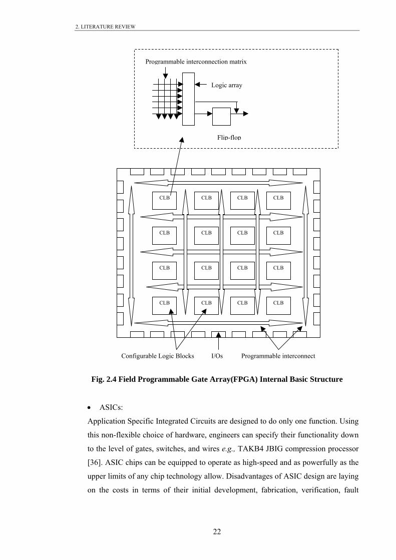
insufficient to implement many tasks. The basic outline architecture of FPGA
devices consists of a number of arrays of logic blocks connected with
interconnection bus lines as shown in Fig. 2.4. Sea-of-gate FPGAs consist of a
system of logic blocks (flip-flops, gates, look up tables) together with some amount
of RAM. FPGAs have embedded processor as well as Giga bit I/O. The
configuration of each of the functions of each logic block and its connections to
other blocks are given by the configuration bit stream loaded from outside the
FPGA device. FPGAs give system designers a broad scale and flexibility for
implementing different algorithms.
21
2. LITERATURE REVIEW
Fig. 2.4 Field Programmable Gate Array(FPGA) Internal Basic Structure
Configurable Logic Blocks Programmable interconnect I/Os
CLB CLB CLB CLB
CLB CLB CLB CLB
CLB CLB CLB CLB
CLB CLB CLB CLB
Flip-flop
Programmable interconnection matrix
Logic array
• ASICs:
Application Specific Integrated Circuits are designed to do only one function. Using
this non-flexible choice of hardware, engineers can specify their functionality down
to the level of gates, switches, and wires e.g., TAKB4 JBIG compression processor
[36]. ASIC chips can be equipped to operate as high-speed and as powerfully as the
upper limits of any chip technology allow. Disadvantages of ASIC design are laying
on the costs in terms of their initial development, fabrication, verification, fault
22

2. LITERATURE REVIEW
detection, and the post-market operating expense if an ASIC chip requires upgrades
for any reason.
FPGAs have advantages over DSPs, since FPGAs permits parallelism, floating-point
operation, and local memory. The parallel reconfigurable technology would have
benefits for problems with a parallel nature and when a speed is a requirement for other
approaches. FPGAs provides a level of both functional and data specialization. They
also extremely useful in quickly permitting generic prototyping. The ability to keep up-
to-date and follow the constantly changing standards in today's advanced technology for
example, the latest wireless, multimedia and image processing algorithms require a new
system-on-chip technology, such as state of the art re-configurable FPGA hardware. In
actual fact, the hardware description languages HDL allows the existing architecture to
track the changing standards, removing necessitates to run brand new algorithms on
yesterday's dedicated hardware architectures [37].
2.5 FPGA Based Architectures
There are three different degrees of FPGA hardware configurations when implementing
the design, static, dynamic and context switching configurations.
Most applications are implemented by applying the static approach. However, dynamic
systems have in recent times become more common. These allow the configuration to
be upgrade when bugs are found or when the functionality of the system is to be
changed.
23

2. LITERATURE REVIEW
Fig. 2.5 Illustration of FPGA Based Architecture on Colour Processing Task
The application area for context switching is in speeding up computation through
dividing the task into smaller processes. If the FPGA can perform Context Switching
CSW operation very fast then rapid swapping between successive processes can give
the FPGA based system a considerable throughput. In Fig. 2.5, to illustrate the three
different configurations, colour processing task consist from processing red, green and
blue colours. If the static configuration were used to processes the task, the FPGA will
permanently keep perform the red, green and black colours processing as a single task.
However if the colour processing task required that a changed is encountered to
replace, as an example, green colour by blue colour, then the Dynamic configuration
have to be used to overcome the changes introduce to the device. If colour processing
task can be partioning into a three separates tasks to be performed one after the other
using different FPGA configuration for each sub-task then the context switching
architecture must be used. In which each colour processing subtask will be processed
separately from other tasks.
P R + P G + P B
P R + P B + P B
P R + P G + P B
P R CSW P G CSW P B
Static
Dynamic
Context switching
Time
24

2. LITERATURE REVIEW
2.5.1 Static FPGA Configuration
In the static FPGA configuration the bitstream file configuration running within the
FPGA is the same throughout the life time of the system. This means no adaptively at
run time. Several attempts to investigate the efficiency of implementing conventional
DCT on FPGA have been carried out; the work conducted in [38] used vector
processing using parallel multipliers for implementation of 2-D DCT on Xilinx FPGAs.
While [39] implemented the DCT algorithm as a part of his successful implementation
for motion JPEG using XCV400 FPGA device. Moreover the author in [40]
implemented the two-dimensional (8x8) point’s discrete cosine transform in Xilinx
XC6200 series of the FPGAs.
The BinDCT algorithm also was implemented on FPGA by [3 - 5] Xilinx XC6200
FPGAs coupled to a TMS320C40 DSP device were used to implement the most
accurate approximation of the fixed point DCT (BinDCT_C1), and the least accurate
approximation BinDCT_C9 algorithms. Work done in [41] has used two
implementation versions of BinDCT, the first one is a simple version of the BinDCT
processor without pipeline. The second one is a pipelined processor. They concluded
that pipelined methods has an area increased of 9.64% when compared to none
pipelined processor implementation within the same FPGA device.
2.5.1.1 Serial Implementation
Despite its slow operation, serial implementations of the BinDCT processor in a static
FPGA configuration mode is fairly simple, requires low gate counts and low bandwidth.
It is therefore suited very well to applications where high speed is less vital. The
implementation of bit-serial adder for example carried by taking the LSB of both
integers and summing first, the carry out if any is kept in a flip-flop, arranging to be add
to the sum of the next higher bit location and so on. The following serial architecture
implantations of the DCT were analysed by Sachidanandan [42]. He implement fully
pipelined bit serial architecture to compute the 8×8 2-D discrete cosine transform with
minimal number of multipliers, he used one bit serial adder, one bit serial subtractor,
one bit pipeline multiplier and dynamic shift register. Timakul [43] has implemented a
1-D DCT based on the work done in [8] for very low bit rate applications, also they
made use of bit-serial computation scheme.
25

2. LITERATURE REVIEW
2.5.1.2 Parallel Implementation
Parallel implementations on the other hand, have faster operation but suffer from
occupying larger areas of the FPGA devices they operate on. As an example of efficient
parallel pipelined implementation of the BinDCT algorithm in hardware [44], the basic
BinDCT architecture is decomposed into five pipelined stages:
BinDCT=E*D*C*B*A
Where A, B, C, D and E are matrices.
Each matrix is associated with one stage in the pipeline architecture. The IDCT
operation is similar but in reverse order. All inputs to the BinDCT processor are signed
integers. The following parallel architecture implantations of the DCT were studied.
Dang et al [45] developed in VHDL a BinDCT processor for wireless video application
using parallel approaches. In their work they divided a 2-D BinDCT in two 1-D blocks.
Each block is implemented in five pipeline stages. Moreover Chuntree and
Choomchuay [46] implemented the binary-lifted DCT that based on the works in [15]
factorisation. Their design was focused on a multiplierless 1-D DCT. Also they
investigated the effect of Different Intermediate Word Length on 512×512 Images.
Schneider-[47] compared the regular and irregular structured algorithms for efficient
hardware realization, investigated the best optimisation for the transition from
algorithms or structured description to hardware architectures. Also he discussed the
criteria to choose between the number of operations and the regularity of the structure.
Hsia et al [48] realized the coefficient-by-coefficient two-dimensional inverse discrete
cosine transform. Their design included a generator of cosine angle index, a pipelined
multiplier, and a matrix accumulator core [48].
26

2. LITERATURE REVIEW
2.5.4 Dynamic FPGA Configuration
Technology has moved with time from using fixed hardware and fixed software
systems, to fixed hardware and reconfigurable software (microprocessor based
systems), to reconfigurable hardware reconfigurable software (FPGA based systems).
When using the dynamic FPGA configuration the design or parts of it is changing from
time to time during run-time operation. Changes introduced to the device representing
rare adaptation.
Dynamic FPGA have been used to implement various applications of the DCT
algorithm. Murphy [3-5] implemented dynamic switching between BinDCT1 and
BinDCT9. Carter et al.[49] implemented a lossless JPEG compression with replacement
of a DCT by a predictor, which estimated the probable value of a pixel from its
neighbours. Larsson and Johnsson, [50] implemented Motion JPEG compression using
DCT. Spillane and Owen [51] examined the applicability of partially reconfigurable
field programmable gate arrays (PRFPGAs) in hardware emulation systems. Kaul et al
[52] proposed new automated temporal partitioning approach for DSP applications.
Current Xilinx Virtex FPGAs family [53] support dynamic partial reconfiguration.
Xilinx provides the users of the partial configurations with four software flow utilities:
• Difference Based Bitgen Flow:
The users of this tool provide two input design files to bitgen, initial and
secondary configurations.
• Modular Design:
It is intended for larger design changes made on the system. To use these tools
two or more partial configurations have to be introduced to the system.
• Partial Mask:
It is intended for the active partial reconfigurations. It needs to be initialising
before using this tool. Active configuration means the new data is loaded to
reconfigure a specific area of the FPGA while the rest of the device is still
running.
• BlockRAM “Savedata”:
It is not intended for use during active reconfiguration, as it can interfere with
BlockRAM operation. It is safe to use it with shutdown reconfiguration.
27

2. LITERATURE REVIEW
2.5.5 Context Switching FPGA Configuration
An important change had been brought to the virtual hardware industry with the
introduction of partially reconfigurable Field Programmable Gate Arrays (PRFPGAs).
Reconfigurable FPGA hardware design has grown to become an important filed of
research. This makes it possible to partition the design in the FPGA by dividing an
outsized designed circuit into smaller circuits or sub circuits. The aim of partitioning is
to allow larger circuits to be implemented by multiple reconfigurations of a single
FPGA. Each consecutive partition reuses the same hardware resources that implemented
the previous active partition. Such temporally partitioned designs are called Run-Time
Reconfigurable (RTR) systems.
This project can use this facility through downloading option one of the proposed
implementation where the nine configurations of the BinDCTs to be downloaded to a
memory on board, and then keep replace the FPGA current BinDCT configuration with
another from the stored configurations reside in the external memory.
Since the context switching undertaken during run time, the total execution time to
perform the task is reduced based on divide-and-conquer approach. The context
switching time would have to be short then to reduce the overhead of switching between
the different configurations.
NEC company has developed a prototype context FPGA chip that is able to store a set
of different configuration bitstreams and make the context switching in a single clock
cycle [54]. Another device capable of storing four configuration on-chip is reported in
[55]. Commercially available FPGAs do not yet provide configuration switching in one
clock cycle and each new configuration would have to be downloaded externally. The
main experience seems to be that today’s FPGAs are still requiring a long time
reconfiguration time, thus making implementations of the Context switching approach
to implement the nine BinDCT configurations is insufficient within the current
technology.
28

2. LITERATURE REVIEW
2.6 Summary
An overview for the DCT algorithms has been investigated. The main derivation,
architectural implementation and the advance hardware being used to implement the
DCT algorithms were revealed. Extensive research has grown up the basic DCT
algorithm from the real part of the Fourier transform. To overcome the extensive
computation of the True DCT (TDCT), new versions of Fast DCT (FDCT) were
proposed. Direct implementations of the FDCT are not so efficient since it consists of
floating-point multiplication and addition units. The multiplierless BinDCT proposed to
overcome this limitation and attain faster implementation through implementing all
floating point multiplications into fixed points shift and add operations.
FPGAs were initially developed for use as reusable prototype devices to reduce
development costs of digital hardware. A review for implementing the DCT and the
BinDCT algorithms within the FPGA devices were given. The static, dynamic, and the
context switching configuration of the FPGA devices are explained.
The overview of the serial and parallel implementations of the static DCT algorthim is
included. The static configuration run within the FPGA is the same throughout the life
time of the system. When using the dynamic FPGA configuration the design or parts of
it is changing from time to time during run-time operation. Current technology
developed by Xilinx Virtex FPGAs family support dynamic partial reconfiguration.
Dividing an outsized designed circuit into smaller circuits and use single FPGA to
switch between their different configurations during run-time is called Context
Switching. Commercially available FPGAs do not yet provide configuration switching
in one clock cycle and each new configuration would have to be downloaded externally.
The next chapter will outline in more details the multiplierless BinDCT algorithm, the
use of this transform approach within the image compression system as will as some of
the image compression ratios result from using both the static and the proposed dynamic
reconfigurable BinDCT algorithm for both loosy and lossless image compression
techniques.
29

3. BINDCT TRANSFORM INTEGERATED PART OF IMAGE COMPRESSION
____________________________________________________________
Chapter 3
BINDCT TRANSFORM INTEGRATED PART OF IMAGE
COMPRESSION ____________________________________________________________ 3.1 Introduction to Basic Principals of Image Compression Communication systems now adays greatly rely on image compression algorithms to
send images and video from one place to another. Every day, a massive amount of
information is stored, processed, and transmitted digitally. The arrival of the biometric
identity concept demand that governments around the world keep profiles of their
citizens, and for businesses to keep profiles of their customers and produce the
information over the internet. Image compression addresses the problem of pressing
large amounts of digital information into smaller packets (by reducing the size of image
and data files) that can be moved quickly along an electronic medium before
communication can take place effectively.
Compressing images results in reduced transmission time and decrease storage
requirements. Whereas uncompressed multimedia files require considerable storage
capacity and transmission bandwidth. The good compression system should be able to
reconstruct the compressed image source or an approximation of it with good quality. It
is an important branch of image processing that is still a very active research field and
attractive to industry. Basic components of a data compression system are illustrated in
Fig. 3.1. There are two different encoding systems in operation within the compression
system, the predictive coding, and the transform coding.
Predictive coding works directly on the input image pixel values as they read into the
system; the spatial or space domain encoder also has the capacity to efficiently expect
the value of the present sample from the value of those which have been processed
previously. So this type of coding has to search for the relationship that governs the tile
30

3. BINDCT TRANSFORM INTEGERATED PART OF IMAGE COMPRESSION
pixels and make a decision for the best way of operating them before the coding process
start.
Transform coding on the other hand uses frequency domain, in which the encoding
system initially converting the pixels in space domain into frequency domain via
transformation function. Thus producing a set of spectral coefficients which are then
suitably coded and transmitted. The background research of this chapter will focus on
the transform coding since the BinDCT algorithm by itself is also transforms the row
image in space domain into spatial frequency domain. The decoder on the other side
must perform an inverse transform before the reconstructed image can be displayed.
The coding technique implemented in this project is the transform coding using
multiplier-less approximation of the DCT algorithms.
Fig. 3.1 Basic Data Compression System
3.2 Inheritance Information Redundancy Reducing the size of the image through compression means reduce the information
content of data set by exploiting the redundancies present in the image. Data
redundancy is a central issue in digital image compression and it may appear in different
forms. If the same information can be represented in two different ways then data
redundancy is an entity which is calculated mathematically by assuming that n1 and n2
denote the number of information carrying units in two data sets that represent the same
information. To know how much the image can be compressed the compression ratio
and data redundancy is calculated by Eq. (3.1). The relative data redundancy of the first
data set n1 can be defined as:
Compression encoding system
Decompression decoding system
Compressed image Reconstructed
Through medium F(X)
Input
Image X
Image Y
31

3. BINDCT TRANSFORM INTEGERATED PART OF IMAGE COMPRESSION
Rd=1-1/Cr (3.1)
Where Cr is commonly known as compression ratio which equal to
Cr = 21
nn (3.2)
According to Eq. (3.2), when the value of n1 = n2 the compression ratio then becomes
one which means that this image cannot be compressed and therefore redundancy in the
image becomes zero. Therefore there is no redundancy occurred in the first image data
set. When the value of n2 << n1 then Cr ∞ and so the redundancy Rd 1, which
indicates that there is a highly redundant data contained within the first image data set.
The only undesirable case could appear indicating the second data image containing
much more data than the original image have when value of the n2 >> n1, and so Rd
- . ∞
The frequency response of the human eye for vertical patterns is similar to the response
for horizontal patterns. For the diagonals on other hand, the response is significantly
reduced. Some compression systems, JPEG among them, are able to take advantage of
this property of the human visual system. They attempt to improve coding efficiency by
preferentially allocating bits to the corresponding transform coefficients to which the
eye is most sensitive. Higher order coefficients can be partially suppressed at
quantization to reflect the lowered response of the eye at the high spatial frequency.
The image brightness at each point depends on both substantial properties of the object
and the lighting condition in the views. Neighbouring pixels of most images are
correlated and so they contain redundant information. Images and audio signals can be
compressed because of the spatial, spectral, and temporal correlation inherent in them.
Data compression is achieved when one or more of these redundancies are exploited
properly.
32

3. BINDCT TRANSFORM INTEGERATED PART OF IMAGE COMPRESSION
3.3 Types of Image Compression There are two basic image compression techniques widely used to exploit the
redundancy in the digital still images, lossless and lossy image compression. Both of
lossy and lossless compression techniques can be done for both types of coding;
predictive and transform coding. The performance measures of image compression
algorithms can be investigated from different perspectives depending on the application
desired, such as amount of compression achieved, objective and subjective quality of
the reconstructed data, relative complexity of the algorithm, or speed of execution.
There are many image compression standards which exist, such as the still-image
compression standard JPEG, H.261 and H.263 videoconferencing standards, and
MPEG-1, -2 MPEG-4 digital video standards.
3.4 Implementations of The Transformation Part The fundamental mechanism of transform coding technique is very simple. In this type
of compression the image samples is taken and transformation is done to alter the
distribution of the values representing the luminance levels. Many of the resulted
transformed samples can either be zeros thus deleted entirely or be quantized and
represented with very few bits. For most of the image samples, the original values will
be similar within the separate tile blocks and occasionally will be significantly different
where an edge occurs. A plot of one luminance value (x) in the block against another (y)
will look like Fig. 3.2 .
Fig. 3.2 Coordinate Rotation For Blocks of Two Sample in (X, Y) Domain And
(C1, C2) Domain.
Y C1
X
C2
33

3. BINDCT TRANSFORM INTEGERATED PART OF IMAGE COMPRESSION
Fig. 3.2 shows coordinate rotation for blocks of two samples in the original spatial data
domain X, Y and the distribution of the samples in the new transform coordinate
transform domain C1, C2 with the bulk of pairs of values located close to the 45
diagonal line.
The basic operation of the transform function is to rotate the coordinates axes from X
and Y to C1 and C2 so that instead of having to keep all sample values in the original
domain with equal resolution, as would have been essential with the original samples
signal, we now have two sets of numbers, one large and one zero or at least for the most
part, fairly small. The new components can be calculated from the original coordinates
using equation derivative below:
C1 =2
)(2 xyx −+ (3.3)
C2=2
)( xy −− (3.4)
The formula can be rewritten to obtain the same divisor for both fractions as:
C1= 222
2 yxx+−⎟
⎠
⎞⎜⎝
⎛ = 2
)( xy + (3.5)
C2=2
)( yx − (3.6)
The inverse operation for the two coefficients to recover the original values X and Y is:
X= 2
)21( CC + (3.7)
Y=2
)21( CC − (3.8)
34

3. BINDCT TRANSFORM INTEGERATED PART OF IMAGE COMPRESSION
If for example the X coordinates = 6 and Y coordinate = 8 then new components will
be:
C1= ( )2
14286
=+
C2= ( )22
286 −
=−
To appreciate the basic functionality of the transform the total input data energy with
the original values x and y denoted by and the new components values C1 and C2
denoted by is calculated. The total samples energy of the original is given by:
OE
NE
22 YXE (3.9) O +=
= (6 + 8 ) = 36 + 64 = 100. OE 2 2
The total samples energy of the new transformed components is given by:
(3.10) 22 21 CCEN +=
The total samples energy of the original is given by:
= NE22
22⎟⎠
⎞⎜⎝
⎛ −+⎟
⎠
⎞⎜⎝
⎛ + YXXY =2
196 + 24 = 98 + 2 = 100.
If we retain only one component of the signal by deleting the smallest component(x) in
the space (x,y) domain then the error e result will be calculated using Eq. (3.11) below:
22
2
YXXe+
= (3.11)
e= 22
2
866+
=10036 =36%.
However deleting the smallest component in the transform domain (C2) then:
35

3. BINDCT TRANSFORM INTEGERATED PART OF IMAGE COMPRESSION
( )22
2
122
CCCe
+= (3.12)
e= 100
2 = 2%
Form Equations 3.7 and 3.8 the approximate values of X and Y when reconstructed
after deleting C2 is
−
Y = ( )2
01−C = −
X = ( )2
01−C = 22
14
x= 7 (3.13)
From equation 3.9 and 3.10 the total transform coefficient energy is the same as the
original data domain energy.
Moving from the space to the transform domain for information broadcasting has
allowed us to keep an approximation to the data vector (7, 7) instead of (6, 8) by
employing only one term in place of two whilst gaining an very less error (2%) as
would have been the case if only one term had been retained in the original space
domain (36%) for this example.
The above transform operation can be set using conventional matrix/vector notation by
writing:
2
121
=⎥⎦
⎤⎢⎣
⎡CC
⎢ ⎥ (3.14) ⎣
⎡11
⎥⎦
⎤−11
⎦
⎤⎢⎣
⎡YX
With inverse:
2
1=⎥
⎦
⎤⎢⎣
⎡YX
⎢ (3.15) ⎣
⎡11
⎥⎦
⎤−11
⎥⎦
⎤⎢⎣
⎡21
CC
The result of the two dimensional transform carried out on blocks of the 8x8 from the
image is a block of transform coefficients of the similar size but having entries values
of widely varying magnitudes as shown in Fig. 3.3. We thus expect to find large
36
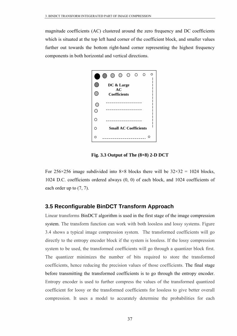
3. BINDCT TRANSFORM INTEGERATED PART OF IMAGE COMPRESSION
magnitude coefficients (AC) clustered around the zero frequency and DC coefficients
which is situated at the top left hand corner of the coefficient block, and smaller values
further out towards the bottom right-hand corner representing the highest frequency
components in both horizontal and vertical directions.
Fig. 3.3 Output of The (8×8) 2-D DCT
For 256×256 image subdivided into 8×8 blocks there will be 32×32 = 1024 blocks,
1024 D.C. coefficients ordered always (0, 0) of each block, and 1024 coefficients of
each order up to (7, 7).
3.5 Reconfigurable BinDCT Transform ApproachLinear transforms BinDCT algorithm is used in the first stage of the image compression
system. The transform function can work with both loosless and lossy systems. Figure
3.4 shows a typical image compression system. The transformed coefficients will go
directly to the entropy encoder block if the system is lossless. If the lossy compression
system to be used, the transformed coefficients will go through a quantizer block first.
The quantizer minimizes the number of bits required to store the transformed
coefficients, hence reducing the precision values of those coefficients. The final stage
before transmitting the transformed coefficients is to go through the entropy encoder.
Entropy encoder is used to further compress the values of the transformed quantized
coefficient for loosy or the transformed coefficients for lossless to give better overall
compression. It uses a model to accurately determine the probabilities for each
DC & Large AC
Coefficients
Small AC Coefficients
37

3. BINDCT TRANSFORM INTEGERATED PART OF IMAGE COMPRESSION
coefficient value and produces an appropriate data width based on these probabilities.
The resultant output code stream of this block will be smaller than the input stream. The
most commonly used entropy encoders are the Huffman encoder, the arithmetic
encoder, and run-length encoding (RLE).
Fig. 3.4 Common Lossless\ Lossy Signal Image Encoder Blocks
In the following sections of this chapter the rule of using the BinDCT algorithm has
been investigated. The results obtained from implementing the BinDCT algorithm
initiate the needs for the novel proposed design. The advantages gained when
implementing the novel system were also outline.
3.5.1 Preliminary Investigations
As explained in section 2.2.3, the BinDCT algorithms have nine configurations. Each
BinDCT have different numbers of add and shift operations as shown in Table 3.1. This
table suggests that the higher the order of the BinDCT configuration algorithm the
higher number of calculations required to conduct the transform operation. Upon this
BinDCT-C2 has fewer calculations than BinDCT-C1, and so with algorithms C3 and C4
up to the configuration C9. The number of shift and add calculation within each
configuration controlled by the lifting step parameters values are specified for each
configuration.
Tran [8] suggested nine different configurations for the dyadic coefficients. These
values are obtained by shortening the corresponding analytical values of the parameter
with different accuracies and by rounding values to dyadic types. These values were
Lossy compression
Lossless compression
BinDCT
Quantizer
block
Entropy Encoder
Compim
ressed age
38

3. BINDCT TRANSFORM INTEGERATED PART OF IMAGE COMPRESSION
inserted into lifting structures indicated by P and U shown in Fig 3.5 for forward
operation and for inverse operation in Fig 3.6 respectively.
x x
39

3. BINDCT TRANSFORM INTEGERATED PART OF IMAGE COMPRESSION
C1 C2 C3 C4 C5 C6 C7 C8 C9
P1 3213
(8+4+1)/32
167
(4+2+1)/16
3213
(8+4+1/32)
167
(4+2+1)/16
83
(2+1)/8 21
21
1 0
U1 3211
(8+2+1)/32
83
(2+1)/8
3211
(8+2+1)/32
83
(2+1)/8
83
(2+1)/8
83
(2+1)/8 21
21
0
P2 1611
(8+2+1)/16
85
(4+1)/8
1611
(8+2+1)/16
85
(4+1)/8
87
(4+2+1)/8
87
(4+2+1)/8 1 1 0
U2 3215
(8+4+2+1)/32
167
(4+2+1)/16
3215
(8+4+2+1)/32
167
(4+2+1)/16 21
21
21
21
0
P3 163
(2+1)/16
163
(2+1)/16
163
(2+1)/16
163
(2+1)/16
163
(2+1)/16
163
(2+1)/16 41
0 0
U3 163
(2+1)/16
163
(2+1)/16
163
(2+1)/16
163
(2+1)/16
163
(2+1)/16 41
41
0 0
P4 3213
(8+4+1)/32
3213
(8+4+1)/32
167
(4+2+1)/16
167
(4+2+1)/16
167
(4+2+1)/16
167
(4+2+1)/16 21
0 0
U4 1611
(8+2+1)/16
1611
(8+2+1)/16
1611
(8+2+1)/16
1611
(8+2+1)/16
1611
(8+2+1)/16
43
(2+1)/4
43
(2+1)/4 21
0
P5 3213
(8+4+1)/32
3213
(8+4+1)/32
83
(2+1)/8
83
(2+1)/8
83
(2+1)/8
83
(2+1)/8 21
21
0
No.
Shifts 23 21 21 19 17 14 9 5 1
No.
Adds 42 39 40 37 36 33 28 24 18
40
1/2
4/sin2π
8/3sin2π
4/sin1π
X[0]
X[4]
X[6] 4x[2]
4x[1]
4x[0]
Table 3.1 Different Dyadic Parameters Values For All BinDCT Configurations
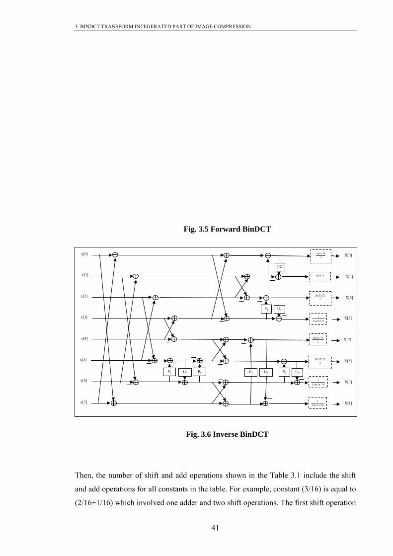
3. BINDCT TRANSFORM INTEGERATED PART OF IMAGE COMPRESSION
Fig. 3.5 Forward BinDCT
Fig. 3.6 Inverse BinDCT
Then, the number of shift and add operations shown in the Table 3.1 include the shift
and add operations for all constants in the table. For example, constant (3/16) is equal to
(2/16+1/16) which involved one adder and two shift operations. The first shift operation
P4 P5U5 P3 U3 P2 U2
P1 U1
1/2
8/3sin21
π
24/sinπ
28/3sin π
216/2sin π
216/3cos π
16/3cos21π
16/7sin21π
4/sin π
X[0]
X[4]
X[6]
X[1]
X[3]
X[5]
X[2]
X[7]
x[7]
x[6]
x[5]
x[4]
x[3]
x[2]
x[1]
x[0]
41

3. BINDCT TRANSFORM INTEGERATED PART OF IMAGE COMPRESSION
shifts integer 2 four places to the right, and second shift operation shift integer 1 four
binary places to the right.
According to Table 3.1 transforming 8 pixels using the BinDCT-C1 requires 23 shifts
and 42 add operations. Therefore for 2D BinDCT-C1 8×8 tile a total of 1040 operation
operands (368 shifts and 672 add operations) are required. However it is required for
each transforming 8 pixels using the BinDCT-C9 1 shift and 18 add operations. Thus
2D BinDCT-C9 8×8 tile will required a total of 304 operation operands (16 shifts and
288 addition operations).
Having established these facts, extending the input stream across (256×256) image will
yield in a significant saving in the number of calculations required. A 256×256 Image
contains 256×32 transform operations based on the fact that in each time segment, 8
input values will be clocked in serial manner. If the processed image was processed
using BinDCT-C1, then the numbers of mathematical operations for each two
dimension forward DCT operation required for whole image in general will be:
No_of_calculations=[2× ( +× operationsshiftno __8 operationsaddno __8× ) ] x
(3.16) tilesimageno __
e.g. using BinDCT1 [2 × (8 × 23 + 8 × 42)] ×32 × 32 = 1064960.
e.g. using BinDCT9 [2 × (8 × 1 + 8 ×18)] × 32 × 32 = 311296.
No_of_calculation_operand_reductions = 1064960 - 311296 = 753664.
The reduction in the number of required calculations for each 256×256 image when
BinDCT-C9 used in place of BinDCT-C1 to process the whole image is approximately
70%
The results obtained from processing the same tile with two different configurations
initiate and therefore invoke further investigation. This research is questioning the
ability of least approximation configurations such as BinDCT-C9 or C8 or C7 to
produce a good quality results compared to best accurate approximation configurations
such as BinDCT-C1 or C2 or C3. The configurations are compared in terms of saving
42

3. BINDCT TRANSFORM INTEGERATED PART OF IMAGE COMPRESSION
execution time by reducing the number of required calculations. And hence this
research investigates when to use which configuration for each tile. To investigate the
quality of the result from each configuration when operate on the same tile, five
different functions each represented by an array of 8 pixel values were used to test the
nine different BinDCT configuration operational characteristics as shown in Figs. 3.7-
3.11. A stream of Ramp, Spike, Constant, Mexican-hat, and Step functions with grey
scale level 0-255 have been applied to each configuration.
Ramp Function
0
50
100
150
200
250
Pixe
l Val
ue
Series1 31 63 95 127 159 191 224 225
1 2 3 4 5 6 7 8
Fig. 3.7 Ramp Function Input Stream
Constant Function
0
50
100
150
200
250
Pixe
l Valu
e
Series1 225 225 225 225 225 225 225 225
1 2 3 4 5 6 7 8
Fig. 3.8 Constant Function Input Stream
43

3. BINDCT TRANSFORM INTEGERATED PART OF IMAGE COMPRESSION
Mexican Hat Function
0
50
100
150
200
250
Pixe
l Val
ue
300
Series1 225 85 170 255 255 170 85 255
1 2 3 4 5 6 7 8
Fig. 3.9 Mexican Hat Function Input Stream
Step Function
0
50
100
150
200
250
Pixe
l Val
ue
Series1 225 225 225 225 0 0 0 0
1 2 3 4 7 85 6
Fig. 3.10 Step Function Input Stream
Spike Funct
0
500
1000
1500
2000
2500
3000
Pixe
l Val
ue
ion
Series1 0 0 0 0 0
1 2 3 4 7 8
0 2525 0
5 6
Fig. 3.11 Spike Function Input Stream
44

3. BINDCT TRANSFORM INTEGERATED PART OF IMAGE COMPRESSION
To compare the ou forward BinDCT
configuration with the true DCT algorithm, the results of the BinDCT must be scaled by
the factors shown in Tables 3.2-3.3, once the scaling factors are considered part of the
forward coefficients calculations, the reverse BinDCT have to be re-adjusted or scaled
back prior to computation of the inverse BinDCT operations. Regardless the scaling
been applied the results from the Inverse BinDCT have to be divided by four to
compensate for the butterfly operation being up-scaled during the butterfly operation.
Forward BinDCT Output Scaling Factor
tput coefficients generated by each of a
X[0] (sinπ /4)/2
X[1] 1/(2sin7π /16)
X[2] 1/(2sin3π /8)
X[3] 1/(2cos3π /16)
X[4] sinπ /4
X[5] (cos3π /16)
X[6] (sin3π /8)/2
X[7] (sin7π /16)/2
Table 3.2 Forward BinDCT Scaling Factor
Reverse BinDCT Output Scaling Factor
X[0] 2/(sinπ /4)
X[1] 2sin7π /16
X[2] 2sin3π /8
X[3] 2cos3π /16
X[4] 1/(sinπ /4)
X[5] 2/(cos3π /16)
X[6] 2/(sin3π /8)
X[7] 2/(sin7π /16)
Table 3.3 Reverse BinDCT Scaling Factor
45

3. BINDCT TRANSFORM INTEGERATED PART OF IMAGE COMPRESSION
The transform coefficients output by each of the nine configurations are compared with
the coefficients generated by the true forward DCT. Figs. 3.12-3.16 shows the Root
Mean Square Error (RMSE) results for each 1D-BinDCT configuration compared to the
true forward 1D DCT for each one of the tested input functions.
RMSE for RAMP Function25
0
5
10
15
20
BinDCT Configuration
RM
SE
Val
ue
Series1 0.79057 0.35355 2.20794 2.34521 2.34521 0.79057 2.66927 12.8111 21.275
1 2 3 4 5 6 7 8 9
Fig. 3.12 Ramp Function RMSE Values For Nine BinDCT Configurations
RMSE for Constant Function
0
0.2
0.4
0.6
1
BinDCT Configuration
Pix
el V
alu
0.8e
Series1 0 0 0 0 0 0 0 0 0
1 2 3 4 5 6 7 8 9
Fig. 3.13 Constant Function RMSE Values For Nine BinDCT Configurations
46

3. BINDCT TRANSFORM INTEGERATED PART OF IMAGE COMPRESSION
RMSE for Mexican Hat Function
0
2
4
6
8
10
12
e
14
BinDCT Configuration
RM
SE V
alu
Series1 0.5 0.79057 0.5 0.79057 0.79057 0.79057 4.60977 4.60977 11.6726
1 2 3 4 5 6 7 8 9
Fig. 3.14 Mexican Hat Function RMSE Values For Nine BinDCT Configurations
RMSE for Step Function
0
20
40
60
80
BinDCT Configuration
RM
SE V
alue
Series1 1.0607 1.8028 3.9843 4.0466 3.2016 4.062 13.757 12.232 70.971
1 2 3 4 5 6 7 8 9
Fig. 3.15 Step Function RMSE Values For Nine BinDCT Configurations
RMSE for Spike Function
0
5
10
15
20
25
30
35
BinDCT Configuration
RM
SE
Val
ue
Series1 0.935414 1.732051 0.935414 1.732051 2.622022 5.556528 7.228416 31.27299 32.2626
1 2 3 4 5 6 7 8 9
Fig. 3.16 Spike Function RMSE Values For Nine BinDCT Configurations
47

3. BINDCT TRANSFORM INTEGERATED PART OF IMAGE COMPRESSION
It is obvious from the Figures above that BinDCT-C7, C8, C9 always produce the
largest RMSE values compared to the configurations BinDCT-C1, C2 and C3 except
when operate on constant function. RMSE values generated by all configurations are
tabulated in Table 3.4. RMSE indicates the quality of produced transformed tile. To
further investigate the relationship between the RMSE result and number of the
mathematical operations required to perform each 1D-BinDCT transform shown in
Table 3.5 was produce.
Input
stream
C1
RMSE
C2
RMSE
C3
RMSE
C4
RMSE
C5
RMSE
C6
RMSE
C7
RMSE
C8
RMSE
C9
RMSE
Ramp
function
0.790569 0.353553 2.20794 2.345208 2.345208 0.790569 2.66927 12.811128 21.274984
Constant
Function
0 0 0 0 0 0 0 0 0
Mexican
Function
0.5 0.790569 0.5 0.790569 0.790569 0.790569 4.609772 4.609772 11.672618
Step
Function
1.06066 1.802776 3.984344 4.046604 3.201562 4.062019 13.756817 12.23213 70.970947
Spike
Function
0.935414 1.732051 0.935414 1.732051 2.622022 5.556528 7.228416 31.272991 32.262596
Table 3.4 RMSE Value Results From Processing The Five Functions Using All
BinDCT Configurations
Input function Lowest
RMSE
Best
Algorithm
Number of
Calculations
Alternative
Algorithm
Number of
Calculations
Constant
Function
0 9 1 shifts+ 18 adds N/A N/A
Ramp
Function
0.35355 2 21shifts+39 adds N/A N/a
Mexican Hat
Function
0.5 3 21shifts+40 adds 1 23shifts+42 adds
Spike
Function
0.935414 3 19shifts+37 adds 1 23shifts+42 adds
Step Function 1.06066 1 23shifts+42 adds N/A N/A
Table 3.5 Input Streams With Most Suitable Algorithm
48

3. BINDCT TRANSFORM INTEGERATED PART OF IMAGE COMPRESSION
In Table 3.5 the best BinDCT configuration for each input function is the one that have
the lowest RMSE value. Results indicated that RMSE are dependant not only upon the
BinDCT configuration being used, but also the frequency content of the input stream.
The alternative algorithm is the one that requires the lower number of calculations
compared to the best algorithm, and at the same time has a very close RMSE value to
the one produced by the best approximation BinDCT Algorithm for the true DCT. Also,
it could have the equal RMSE value to the best selection but require higher number of
calculations. Hence some times using the alternative algorithm instead of the best
algorithm will save a lot of calculations, at the expense of very small decrease in quality
compared to the best algorithm. The alternative will be chosen if it has less number of
calculations, but having slightly higher RMSE value from the best one.
Based on the results from the constant input function in Table 3.4, the RMSE values are
the same across all algorithms (BinDCT-C1 to BinDCT-C9). The justification to use
BinDCT-C9 instead of BinDCT-C1 comes from the advantage gained when processing
forward 256×256 images with the same image quality. Thus leads to speed up the
processing time and obtaining higher compression ratio. Coding gain and the
compression ratio will be different when using different configurations as will be shown
in the following section.
The work done in [3] investigated the BinDCT coding gain which is between the most
accurate BinDCT-C1 and the least accurate BinDCT-C9 forward transform coefficients.
The research indicated that for high frequency input data, higher compression ratios
were obtained using BinDCT-C1 compared to BinDCT-C9. For low frequency content
of inputs BinDCT-C9 generated greater loss-less compression ratios than BinDCT-C1.
3.5.2 Lossless Compression
Error free image compression approaches address methods of information saving, but in
fact such compression preserves only the information in the sampled data totally
ignoring the loss of information that results from digitizing or sampling the analogue
signals to create the digital image. This kind of compression is useful in image
archiving as storage of legal or medical records.
49

3. BINDCT TRANSFORM INTEGERATED PART OF IMAGE COMPRESSION
From Fig. 3.1 in the introduction if the reconstructed image Y is an exact replica of the
original input image X, we call the algorithm applied to compress the image X and the
decompressed image F(X) to be lossless. The most popular performance measure of
image compression is the compression ratio. This can be calculated by the number of
bytes needed to store the compressed image compared to the number of bytes needed to
store the original image. To investigate the two dimensional dynamic BinDCT
compression ratio, the heavily used image processing Lena image was transformed
using static BinDCT, and the proposed Dynamic BinDCT transforms. This was
conducted using C program written by the author. The results obtained indicate the
number of zero coefficients obtained through performing the appropriate two
dimensional transform on Lena image. Even though the most suitable way of
calculating the compression ratio for a particular image, it requires more than only the
transformed image. Hence the distribution of the transform coefficients such as zeros
have very important rule on the image compression coding and decoding. The aim of
this project is to improve some aspect of the image compression through minimising the
number of calculation when using Dynamic reconfigurable BinDCT from BinDCT-C1
to C9 to process the image, therefore we will use number of zeros generated by al
configurations as a measure of compression ratio for this research.
Hence an investigation has been carried out to inspect the effect of use of each BinDCT
configuration when perform the whole image on the compression ratios resulted. Lena
image has been processed by BinDCT-C1 to BinDCT-C9 which I referred to as a static
BinDCT implementation as well as with the dynamic BinDCT system. The number of
zero coefficients generated by the transform has also been noted in Table 3.6.
Compression ratios for all results from each configuration according to Eq. 3.1 above
when n1 is the (256×256) pixels image before transformation and n2 is the remaining
pixels after transformation is also calculated in the Table 3.6 for lossless compression.
Fig. 3.17 shows the nonlinear relationship obtained between the compression ratio and
the static BinDCT configurations C1 to C9 used to process the same image as well as
the Dynamic BinDCT system denoted by DCT type number 10 in all Figures. The
biggest ratio 1.157000865 was obtained through using Dynamic BinDCT algorithm
where more than one configuration is used to process the image during run time. Since
the image compression ratio calculation depends on the number of zero coefficients
50

3. BINDCT TRANSFORM INTEGERATED PART OF IMAGE COMPRESSION
generated. Fig. 3.18 emphasise that the novel dynamic BinDCT processor
implementation generates the biggest number of zero coefficients, i.e., 8893.
Zero Coefficient Nonzero Coefficient Compression ratio RMSE BinDCTc1 8866 56670 1.156449621 1.236464 BinDCTc2 8822 56714 1.155552421 1.318841 BinDCTc3 8701 56835 1.153092285 1.38349 BinDCTc4 8728 56808 1.153640332 1.410406 BinDCTc5 8769 56767 1.15447355 1.449532 BinDCTc6 8799 56737 1.155083984 1.523343 BinDCTc7 8653 56883 1.152119262 2.841358 BinDCTc8 8422 57114 1.147459467 5.604115 BinDCTc9 7879 57657 1.136652965 8.448665 Dynamic BinDCT 8893 56643 1.157000865 1.26789
Table 3.6 Results of Lossless Compression on Lena Image.
Lena Compression Ratio
1.125
1.13
1.135
1.14
1.145
1.15
1.155
1.16
1 2 3 4 5 6 7 8 9 10
BinDCT Type
Com
pres
sion
Rat
io
compression ratio
Fig. 3.17 Lossless Compression Ratio For Nine Configurations And The Dynamic
BinDCT For Lena Image
51

3. BINDCT TRANSFORM INTEGERATED PART OF IMAGE COMPRESSION
Lena Zero Coefficients
760078008000
8400860088009000
Num
ber
Zer
os
72007400
8200
1 2 3 4 5 6 8
BinDCT Type
of
7 9 10
Series1
mmonly used objectives
measures are RMSE, Signal to Noise Ratio (SNR), and Peak Signal to Noise Ratio
SNR). The one being focus upon in this project was RMSE which can be calculated
usi
Fig. 3.18 Lossless Zero Coefficients For Nine Configurations And The Dynamic
BinDCT For Lena Image.
The difference of the reconstructed pixels from the original image is called the
distortion. Quality of the image could be very subjective based on human perception or
can be objective using mathematical assessment. The most co
(P
ng Eq. (3.17). Where −
Y (i,j) represents the processed image by one of the BinDC
sents the output coefficients
T
configurations and Y(i,j) repre of forward true DCT.
RMSE = ( )2
0 0,,1 ∑∑
= =
ean square error (RMSE) of Fig. 3.19 for the BinDCT
−
⎥⎦⎤
⎢⎣⎡ −
M
i
N
jjiYjiY
MN (3.16)
The relationship of the root m
configurations C1 to C9 dose not generate similar behaviour for the compression ratio
relationship. However the only exception from the relationship was the dynamic
BinDCT system where it also usefully produces RMSE 1.26789, this value considers
very close to the RMSE of the best approximation of the true DCT BinDCT-C1 and too
far from the least approximation of the true DCT BinDCT-C9.
52

3. BINDCT TRANSFORM INTEGERATED PART OF IMAGE COMPRESSION
Lena RMSE Result
0
1
2
3
1 2 3 4 5 6 7 8 9 10BinDCT Configuration
RM
4
5
6
7
8
9
SE V
alue
Series1
Fig. 3.19 Lossless RMSE Values For Nine Configurations And The Dynamic
BinDCT For Lena Image.
The work done on using the novel BinDCT system with lossless compression systems
demonstrate its efficiency to be used through generating higher compression ratios and
wer RMSE values.
e concept of compromising the accuracy of the reconstructed image in
xchange of increasing the compression ratio. The principal difference between these
two approaches is the p o b c
are simply the scaled m h m n alues of th xels in the image block,
therefore uniformly qua e s y th
are formed as weighted sums and differences of pixels in the tile.
lo
Another test has been carried out to a constant image. All the pixels in each tile of the
image have the same value. The compression ratios obtained for all nine configurations
has the same number of zero coefficients which are 64512. Therefore the compression
ratio is 64. Tiles with low frequency contents resulted in compression ratios that are
higher than processing tiles with high frequency contents.
3.5.3 Lossy Compression
Unlike the error free approaches outlined in the previous section, loosy encoding is
based on th
e
resence r a sen e of the quantizer block. The DC coefficients
ean of t e lu ina ce v all e pi
ntiz d u uall wi a word length of 8 bits. The AC coefficients
53

3. BINDCT TRANSFORM INTEGERATED PART OF IMAGE COMPRESSION
Lena image used again this tim e
implementation of static BinDCT and the novel proposed dynamic reconfigurable
BinDCT system in term ss . The quantization matrix used to test the
BinDCT system is sho i a 3 T e e lso tabulated in Table
3.7. For loosy compression BinDCT-C1 produces the highest ratio 4.578774541, while
least approximation BinDCT-C9 produce the lowest 3.993662401. However the
dynamic BinDCT syste very close to the ratio
obtained by C1 as shown in Fig. 3.20. The nonlinear relationship obtained between the
comp io an o C ces
same ell as the ic BinDCT s enoted by mb
in th re.
The uantizatio alculating the value ge all
configurations implementation and the dynami guration ar ig.
Quantization in general reduced the RMSE val rated for a ns
the detail system
where also produced an RMSE value very close to the RMSE value of the best
approximation of the DCT BinDCT1 and too far away from the least approximation of
the DCT BinDCT9. According to this result the choice to use BinDCT-C1 or the
dynamic BinDCT system will take in considerations the number of calculations to be
saved when using the novel dynamic system over the static BinDCT-C1 to operate on
the image.
16 11 10 16 24 40 51 61
e to inv stigate the affect of quantization step on the
s of compre ion ratio
wn n T ble .6. he r sult obtain d is a
s
m produce compression ratio less but
ression rat d the BinDCstatic T confi ns C1 tguratio 9 used to pro s the
image as w Dynam ystem d DCT type nu er 10
e same Figu
effect of q n on c RMSE nerated for static
c confi e shown in F 3.21.
ue gene ll configuratio since
ed information were omitted. However the novel dynamic BinDCT
12 12 14 19 26 58 60 55
14 13 16 24 40 57 69 56
14 17 22 29 51 87 80 62
18 22 37 56 68 109 103 77
24 35 55 64 81 104 113 92
49 64 78 87 103 121 120 101
72 92 99 95 98 112 100 103
Table 3.6 Quantization Matrix Used
54

3. BINDCT TRANSFORM INTEGERATED PART OF IMAGE COMPRESSION
Zero Coefficients ratio RMSE Nonzero Coefficients Compression
BinDCTc1 51223 14313 4.578774541 0.029037BinDCTc2 51200 14336 4.571428571 0.036907BinDCTc3 51193 14343 4.569197518 0.037425BinDCTc4 51150 14386 4.555540108 0.041144BinDCTc5 51137 14399 4.551427182 0.043045BinDCTc6 51142 14394 4.553008198 0.056156BinDCTc7 46421 19115 3.42851164 0.115065BinDCTc8 50337 15199 4.311862623 0.242851BinDCTc9 49126 16410 3.993662401 0.243776
Hybrid BinDCT 50735 14801 4.427808932 0.030397
Table 3.7 Quantized Lena Image For Loosy Image Compression
Lena Compression Ratio
00.5
11.5
22.5
33.5
44.5
5
pres
sion
Rat
io
1 2 3 4 5 6 7 8 9 10
BinDCT Type
Com
Series1
igurations And The Dynamic Fig. 3.20 Lossy Compression Ratio For Nine Conf
BinDCT For Lena Image
55

3. BINDCT TRANSFORM INTEGERATED PART OF IMAGE COMPRESSION
Lena Loosy RMSE
0
0.05
0.1
0.15
0.2
0.25
0.3
Pixe
ls V
alue
1 2 3 4 5 6 7 8 9 10
BinDCT Type
Series1
Fig. 3.21 Lossy RMSE Values For Nine Configurations And The Dynamic BinDCT
For Lena Image
s Compression ossless image compression techniques are the only acceptable means of data reduction
The same constant image carried out to investigate the use of the novel Dynamic
BinDCT with lossless technique is also done with the lossy image compression
technique. The compression ratios obtained for all nine configurations are the same as
the number of zero coefficients generated is equal for lossy and lossless algorithms.
Therefore the compression ratio is 64.
3.6 Implementations of LosslesL
for numerous applications. Error free compression is commonly used in archival of
medical or business documents. It is also used with processing of LANDSAT imagery,
where both the use and cost of collecting the data makes any loss undesirable. It is also
preferred for artificial images such as technical drawings, icons or comics. The popular
ZIP, PNG, GIF files format uses lossless image compression techniques.
56
3. BINDCT TRANSFORM INTEGERATED PART OF IMAGE COMPRESSION
3.7 Implementations of Lossy Compression Lossy image compression is useful in applications such as broadcast television,
Videoconferencing, and facsimile transmission. In general it is most commonly used to
compress multimedia data such as video and still images where a certain quantity of
error is a satisfactory trade off for increased compression ratio. In JPEG algorithm, for
each 8×8 image data blocks there is one DC and 63 AC coefficients. All coefficients are
then uniformly quantised with a step size defined by quantization matrix range from 1
to 255 and are predefined by psycho visual tests. The two dimensional array of AC
coefficients are reordered into a one dimensional zig-zag scan.
3.8 Summary The principal objectives of this chapter are to present the theoretic foundation of the
digital image compression. Digital image compression applications are common place
today. They can be found in our daily life from simple to very complicated systems,
such as the digital TV, computers, Internet, multimedia mobile phones, MP3 players,
and machine vision systems. The sufficient storage space, large transmission bandwidth,
and long transmission time required by uncompressed files are behind the needs for
more efficient image compression techniques. Reducing the size of the image through
compression means reducing the information content of a data set by exploiting the
redundancies present in the image file.
The two basic image compression techniques widely used to exploit the redundancy in
the digital still images are discussed in this chapter. The transformation part of both
lossless and lossy image compression techniques have been tested using the BinDCT
algorithm.
BinDCT algorithms have nine configurations. Each algorithm has different numbers of
add and shift operations. Since the number of shift and add operations implemented in
each configuration is different, all BinDCT configurations have been investigated to
calculate the amount of reduction in operations when different algorithm is performed
for the same image. The reduction in the number of operand execution for each
256x256 Lena image when BinDCT-C9 used in place of BinDCT-C1 to process the
whole image is approximately 70%.
57

3. BINDCT TRANSFORM INTEGERATED PART OF IMAGE COMPRESSION
The effect of using the Dynamic reconfigu able BinDCT system to generated the best
compression ratio compared with bo oosless techniques were addressed.
he biggest ratio was obtained through using the novel dynamic BinDCT algorithm
sy s
te e
erformed well and produced compression ratios very close to the best approximation
n C9 configuration. However the dynamic BinDCT system also
r
th Lossy and L
T
stem with RMSE value very close to the value produced by BinDCT-C1 for lossles
chnique. Compression ratio produced by the dynamic BinDCT with lossy techniqu
p
C1 and far better tha
produced RMSE very close to the RMSE of the best approximation of the DCT
BinDCT1 and too far from the least approximation of the DCT BinDCT9.
Lossy and Lossless Image compression techniques generated the same image
compression ratio when operating on constant tiles. This result can be used to suggest
better performance image compression systems.
58

4. MODELLING AND SELECTION TECHNIQUES ALGORITHMS
Chapter 4
MODELLING AND SELECTION TECHNIQUES ALGORITHMS
_________________________________________________________
ntroduce the design of the mechanisms developed to detect and
erefore decide which configuration best matches the incoming tile during run time
operation. This pre-processin ieved the
incoming tile. The proposed selection-based techniques certainly involve one of the
ell known image processing techniques known as texture image processing.
forward BinDCT operation, so the system needs to pass
n the output of the pre-processing stage, assess and classify the output to which
riate.
4.1 Introduction Image analysis involves investigation of the image data for a specific application to
determine how can be the used to extract the information required. Therefore the
relationship between different pixels in the image can be used. The main objectives of
this chapter is to i
th
g stage ach by analysing the frequency content of
w
The novel selection techniques discussed here works on local information contained
within each tile of the image separately. The results from this locality search will output
a piece of information to be used for the next stage, since the next operation to be
conducted in this design is the
o
BinDCT configuration the processed tile most approp
In the following sections the theoretical background for each sub-block makes the
design as well as its mathematical derivation is presented. Moreover the results obtained
when tested the proposed novel selection techniques where also analysed towards the
end of this chapter.
59

4. MODELLING AND SELECTION TECHNIQUES ALGORITHMS
4.2 Methods To Exploit Information From The Source Image
c procedure.
ccording to Shannon, if a random event E that occurs with probability P(E) is said to
old I(E) units of information. Then quantity I(E) is often called self-information, and is
iven by Eq. (4.1):
I(E )=log
The essential mathematical structure for performing data compression using statistical
means is described in the well-established information theory by Shannon [56]. This
theory supplies the basic tools needed to work with information representation and
manipulation directly and quantitatively.
4.2.1 Elements Of Information Theory
The generation of information can be represented as a probabilisti
A
h
g
)(1EP
=-log P(E) (4.1)
Where the amount of information qualified to event E is inversely associated to the
probability of E. Based on Eq. (4.1) if the probability P(E) value becomes very small,
equals or approaches zero, this indicate that the event E is less possible to occur, and
hence I(E) becomes very large. According to that ation to represent
the event E will then be large.
bined probability of grey-level pairs in an
age. The co-occurrence matrices treated as another form of a transform function,
which transform the source image into another presentation. The extracted features from
the matrix have always been used widely by many im processing applications, the
common use encountered due to the fact that the constructed matrix is symmetric and
when normalised elem values betwe e valu -0). Haralick [57] proposed
14 different statistical features that can be cted f
contrast, entropy and
the amount of inform
4.2.2 Gray Level Co-occurrence Matrix (GLCM)
GLCM uses the elements of the information theory and is defined as a tabulation for
how frequently different combinations of pixel grey levels occur in a window within an
image. It is an approximation of the com
im
age
ent are en th es (1
extra rom the GLCM such as energy,
homogeneity
60
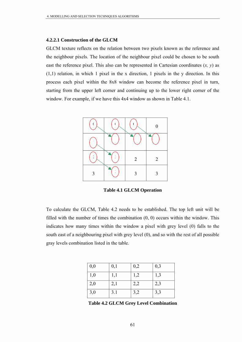
4. MODELLING AND SELECTION TECHNIQUES ALGORITHMS
4.2.2.1 Construction of the GLCM
GLCM texture reflects on the relation between two pixels known as the reference and
e neighbour pixels. The location of the neighbour pixel could be chosen to be south
ast the reference pixel. This al can repr ente in Cartesian coordinates (x, y) as
,1) relation, in which 1 pixe the dire on, ixels in the y direction. In this
rocess each pixel within the 8 w ow n become the reference pixel in turn,
tarting from the upper left corner and continuing up to the lower right corner of the
window. For example, if we have this 4x4 window as shown in Table 4.1.
s to the
south east of a neighbouring pixel with grey level (0), and so with the rest of all possible
gray levels combination listed in the table.
0,0 0,1 0,2 0,3
th
e so be es d
(1 l in x cti 1 p
p 8x ind ca
s
Table
Table 4.1 GLCM Operation
To calculate the GLCM, Table 4.2 needs to be established. The top left unit will be
filled with the number of times the combination (0, 0) occurs within the window. This
indicates how many times within the window a pixel with grey level (0) fall
1,0 1,1 1,2 1,3
2,0 2,1 2,2 2,3
3,0 3.1 3,2 3,3
Table 4.2 GLCM Grey Level Combination
0 0 0 0
1
1
1
1
2
2
2
2
3 3 3 3
0
1
0
11
22
3
0
1
61

4. MODELLING AND SELECTION TECHNIQUES ALGORITHMS
The e
occurre Table 4.3:
outh eastern neighbour is also (0) occurred. Three
tim t n h eastern neighbour is (1), also (0) times the
reference pixel is (0) and its south eastern neighbour is also (2). (0) times the reference
pixel is (0) and south eastern neighbour is (3). And so on for the rest of the table.
CM commonly implemented with some degree of rotation. This is usually achieved
r sultant fill of the matrix for the south east (1, 1) relationship gives this co-
nces matrix shown in
0 3 0 0
0 0 3 0
0 0 0 3
0 0 0 0
(a)
Table 4.3 GLCM Matrix
The first line of the Table 4.3(a) can be interpreted as (0) time in the tested window that
the reference pixel is (0) and its s
es he refere ce pixel is (0) and its sout
GL
by recalculating the GLCM array for different angles followed by combining the result
of breaking up angles. If the GLCM is calculated with symmetry then only angles up to
180 0 degrees needs to be considered and the four angles 0 0 , 45 0 , 90 0 , 135 0 are an
effective choice. All the calculations made have used 1 pixel as offset between the
reference pixel and its neighbour as a separation between the two pixels. The results are
then combined by averaging the features calculated for each of the four angles.
62

4. MODELLING AND SELECTION TECHNIQUES ALGORITHMS
Examples:
• x = 1 and y = 0 means the relationship between the reference and right
neighbouring pixel.
• x = 0 and y = 1 means the relationship between the reference and bottom
neighbouring pixel.
• x = 1 and y = 1 means the relationship between the reference and right bottom
neighbouring pixel.
x = 2 and y = 0 means the relationship between the reference and right
o on.
The angle determines which neighbouring pi
performing the entropy operation.
• Angle 0 means the left east pixel.
• means the bottom pixel
atrix needs 255×255 entries. Therefore for
tion and to decrease drastically memory
requirements normally 8 grey levels are sufficient. This grey level values can be
obtained by dividing the values of the pixels in the incoming window by 32. So instead
of expecting the max m grey scale le
becom He hes ult new GLCM tri ith 4 entrie
GLCM technique has been implemented in FPGA chip, because the GLCM is highly
computational intensive, authors [58-60] has investigate the use of the FPGA to
accelerate the computat features using Xilinx
XCV2000E Virtex FPGA.
•
neighbouring pixel that is far two pixels from the processed pixel.
• x = 1 and y = 0 is equivalent to radius = 1 and angle = 0o. And s
xel to take in consideration when
0
0Angle 90
• Angle 45 0 means the bottom-left pixel
• Angle 135 0 means the bottom right pixel
Calculating GLCM for 256 grey levels in a window requires an enormous processing
time and memory, in this case the GLCM m
the purpose of this research investiga
imu vel value for each window to be 255 it will
e 7. nce t e res s in a ma x w 9 s.
ion of the GLCM and some texture
63

4. MODELLING AND SELECTION TECHNIQUES ALGORITHMS
4.2.3 Normalisation
The co-occurrences matrix needs to be normalised. This final step of normalisation
performed for the reason that the measures required the GLCM units to hold a
probability rather than a count for how many times the particular gray level combination
occurs. The probability of the event JX that the source will produce is P(xj) , and the
sum of the all the probability of all the events is given by Eq. 4.2:
∑=
a matrix. Normalisation equation used in
is project to normalise the GLCM entries is presented in Eq. (4.3):
=j
jjxP
01)( (4.2)
There are many different ways of normalising
th
∑−= 1
=
,, N
jiji
V
VP (4.3)
on Operation
0/9 3/9 0/9 0/9
0,,
jiji
Where (i) represent the row and (j) represents the column so (i) and (j) keep track of the
entry values by their horizontal and vertical position. V is the value in the unit i, j of the
GLCM, while Pi,j is the probability for the unit i, j. And N is the number of rows or
columns. Suppose that we have the GLCM matrix shown in Table 4.5(a), the total
occurrences were 3+3+3=9 and thus each GLCM cell will be divided by the 9, so
(1/3+1/3+1/3) =1 as required by Eq. (4.2)
=
(a) (b)
Table 4.5 Normalizati
0/9 0/9 3/9 0/9
09 0/9 0/9 3/9
0/9 0/9 0/9 0/9
0 1/3 0 0
0 0 1/3 0
0 0 0 1/3
0 0 0 0
64

4. MODELLING AND SELECTION TECHNIQUES ALGORITHMS
4.2.4 Entropy
Having calculating the GLCM and the matrix normalising step done, the next stage is to
calculate the Entropy. Entropy is a quantitative entity verifies the amount of the
information enclosed within each window. For this work, the window size is equal to a
tile size which 8×8 pixels. The average information per source output is calculated by
dding up the information quantity of all elements generated by a source multiplied by
their probability of occurrence. Entropy is well known as the uncertainty of the source.
It defines the average amount of information obtained by observing a single source
output. Entropy is calculated using Eq. (4.4):
a
( )∑−
=
matrix which is equal to 7, P is the probability or the value of cell i,j which is
obtained from the normalised GLCM. ln is the "natural logarithm" and uses a base close
to (2.718). The smaller the value of Pi,j; the less common is the occurrence of that pixel
combination and the larger is the absolute value of ln(Pij ). The (-1) multiplier in the
entropy equation makes each result positive. Therefore, the smaller the Pij value, the
greater the weight, and the greater the value of -[Pij * ln(Pij )]. Higher entropy values
means that more information is associated with the source and more frequency content
variation across the tile and less uniform distribution of the pixel values across the tile.
4.2.5 Homogeneity
Homogeneity uses also the GLCM matrix similar to the entropy. Homogeneity is
largely related to the local information extracted from an image and indicates how
uniform ilar. Homogeneity plays an
important role in image segmentation since the result of image segmentation would be
several homogeneous regions. The more regular the local region surrounding a pixel is,
the larger the homogeneity value the pixel has.
The value of the homogeneity at each location of an image has a range from (0 to 1), so
according to our investigation the tiles that have great pixel values variation tend to
ave smaller homogeneity value, while the constant tiles that have low pixel variation
−=1
0,,ln,
N
jijPijPiE (4.4)
Where E is the entropy value calculated for each tile, N is a row or column of the
GLCM
a region is and the degree to which pixels are sim
h
65

4. MODELLING AND SELECTION TECHNIQUES ALGORITHMS
should have homogeneity value close to 1. Homogenity can be define as a composition
f two components: standard deviation and discontinuity of the intensities. It can also be
alculated when related to the GLCM using weights values by the inverse of the
ontrast weight. GLCM are already a measure of commonness of occurrence.
omogeneity is calculated using Eq. (4.5):
o
c
c
H
( )∑−
= −+=
1
0,2
,
1
N
ji
ji
jiPH (4.5)
.3 Entropy Operational Procedures
he experimental work is carried out here for each 8×8 tile of the Lena image. The tiles
ave to go through different steps before finally written out. The system construction is
ased on the operational procedures needed to get the system to reconfigure the
roposed generic BinDCT system. The flow graph of this operation is shown in Fig.
.1.
4
T
h
b
p
4
66

4. MODELLING AND SELECTION TECHNIQUES ALGORITHMS
Fig. 4.1 The Flow Graph of The Entropy Operation
The first step of the algorithm is to buffer the first 64 pixel values of the incoming tile
and hold the system waiting for this tile to be processed completely. This operation will
be followed by computing the GLCM for the tile. The computed GLCM will then be
normalised and used with one of the two texture feature selection-based techniques
needed as explained before. The tile will be processed first with the true DCT. Then the
same tile will be processed by each one of the nine BinDCT algorithms separately. The
Yes
No
Entropy values complete Image
BinDCT Processors 1 2 3 4 5 6 7 8 9
Attach each entropy and homogeneity values to each Tag
Set limits and boundaries
Entropy Files 1 2 3 4 5 6 7 8 9
Entropy single value 1 2 3 4 5 6 7 8 9
Homogeneity values complete
Image
Set limits and boundaries
Homogeneity Files 1 2 3 4 5 6 7 8 9
Homogeneity single value 1 2 3 4 5 6 7 8 9
Calculate entropy
Incoming tile
Tag 1 to 9
Lowest RMSE value
>?
Calculate Homogeneity For each tile
Start
End of file
Finish
True DCT
67

4. MODELLING AND SELECTION TECHNIQUES ALGORITHMS
output coefficient values of each BinDCT configuration will be compared to the output
of the True DCT to calculate the RMSE using Eq. (3.16) of section 3.5.2
The information contained within the GLCM and the normalised GLCM will then be
assed further to calculate the entropy value. The entropy or homogeneity for the same
tile will be calculated and stored in one of the nine files named entropy1 to entropy9.
Different entropy and homogeneity files exist following the nine different BinDCT
c
for each particular tile.
Once the RMSE calculation was performed, the RMSE value will decid which BinDCT
configuration produces the lowest RMSE value, which means that this configuration has
been chosen as the best approximation to the true DCT. Therefore, it raises a flag to
mark the suitable configuration algorithm number. Each processed tile will have an I.D
number between 1 and 9 based on RMSE values obtained. The calculated entropy for
the same tile will search for this flag and the entropy value will be stored to a specific
file accordingly. These procedures should continue until processing the complete tested
image. The output of this stage is nine different entropy files, each of which represents
one particular BinDCT configuration that operates on the tile contained by the entropy
files.
The procedure is repeated to process 20 different images, and obtain their entropy files.
The entropy values within each file will be average to produce a single value to
represent this particular configuration number results form processing the 20 images
[Appendix]. Thus file entropy1 will be assessed and all the values will be averaged
inside the file, by doing so we obtain one single entropy value to represent all possible
entropy values for all tiles processed by as an example BinDCT configuration 1. The
purpose of this is to get a more accurate approximation to cover wider variation of the
entropy values that could appear as shown in Table 4.6. The produced single entropy
value for each particular configuration will be average again for the 20 images as shown
in Fig. 4.2. Averaging between the neighbouring points in the figure helps in creating
two sets or value limits for each configuration as shown in Fig. 4.3. Fig. 4.4 shows more
details the differences in the values between each average point representing each
configuration. The calculated nine different entropy values will be then used as a
p
onfigurations allocation. The allocation has been assigned based on the RMSE value
68

4. MODELLING AND SELECTION TECHNIQUES ALGORITHMS
database in the system and therefore use them as set of boundaries that control the data
flow. All new calculated entropy values will be compared against thresholds checking
points. Based on those thresholds one of the BinDCT configurations will be activated.
This stage forms the input to the hybrid or dynamic generic BinDCT processor.
Table 4.6 Entropy Values Results From Processing 20 Images For Nine BinDCT
Configurations
69

4. MODELLING AND SELECTION TECHNIQUES ALGORITHMS
Fig. 4.2 Entropy Average For 20 Images
Fig. 4.3 Comparison Between The Two Average Sets
70

4. MODELLING AND SELECTION TECHNIQUES ALGORITHMS
Fig. 4.4 Differences Between The Entropy Values And The Average For the Same
Points
The proposed system then works by obtaining these limits for each BinDCT
configuration. This technique allows us to e based on the
entropy value for each tile rather than the use of RMSE value. The data flow diagram
shown in Fig. 4.5, outline the procedures n ds to be followed to process any new still
image without the need to go through the data flow shown in Fig. 4.1 since all the work
done on the previous stage was to establish the threshold limits.
continue processing this tim
ee
71
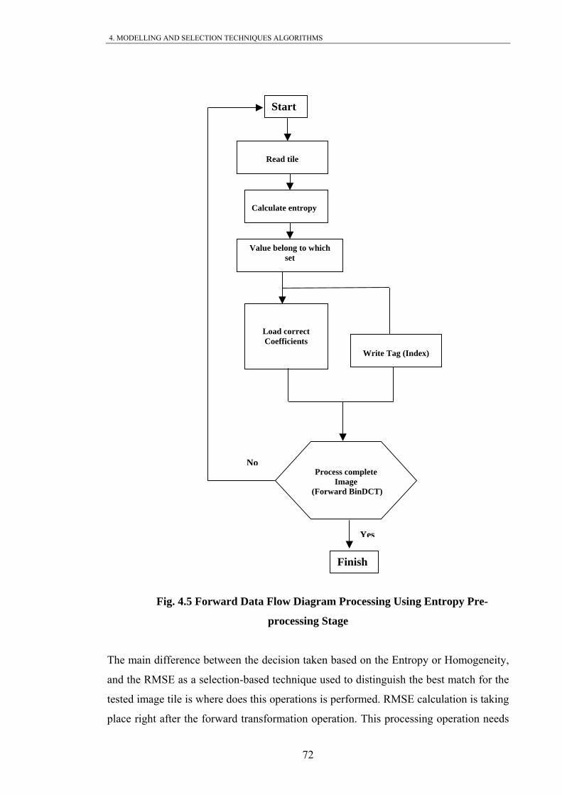
4. MODELLING AND SELECTION TECHNIQUES ALGORITHMS
Fig. 4.5 Forward Data Flow Diagram Processing Using Entropy Pre-
processing Stage
The main difference between the decision taken based on the Entropy or Homogeneity,
and the RMSE as a selection-based technique used to distinguish the best match for the
tested image tile is where does this operations is performed. RMSE calculation is taking
place right after the forward transformation operation. This processing operation needs
No
Start
Read tile
Calculate entropy
Value belong to which set
Write Tag (Index)
Load correct Coefficients
Finish
Process complete
Image (Forward BinDCT)
Yes
72

4. MODELLING AND SELECTION TECHNIQUES ALGORITHMS
to involve all the nine configurations of the BinDCT every time with every single tile in
e image. The decision then will be made based on the lowest RMSE value. On the
ther hand calculating the entropy or the Homogeneity value for each incoming tile
rst, and place it within the limit that fit the calculated entropy value enable us to select
etween different configurations without the need to do the transform of the nine
inDCT configuration for the same incoming tile, instead load the parameter
oefficients for the selected configuration directly. This obtained pre-processing step is
hat this proposed novel work aimed for. During the transform operation another file
as been written out at same time, this file work as tag or identification number belongs
r each tile in the file. From which we can tell which BinDCT configuration was
elected to perform on this specific tile of the image.
he inverse DCT transform itself can perform the tile selection-based technique using
e nine different inverse BinDCT configurations and hence constructing a dynamic
eneric Inverse BinDCT processor. The tag file created during the forward operation
an be used. Reading the file contains information on which BinDCT configuration
ere selected or used to process this tile during transformation stage will result in
loading the same parameter coefficients du
hould be able to switch and selected best InvBinDCT configuration that suits each tile
uring run time too. Thus advantage of the Re-configurablel system can be used during
e compression and decompression stage of the transform as explained in Fig. 4.6.
th
o
fi
b
B
c
w
h
fo
s
T
th
g
c
w
ring the inverse operation. Thus the system
s
d
th
73

4. MODELLING AND SELECTION TECHNIQUES ALGORITHMS
Read Tag (Index)
Load correct coefficients
(Inverse BinDCT)
Write to file
Start
ig. 4.6 Inverse Data Flow Diagram Processing Using Pre-processing Stage
he same pre-processing data flow design is done for calculating the entropy can be
sed to construct another system, which is based on the homogeneity value this time. It
has to dynamically switch and re-configure nDCT processor with the appropriate
para with
each tile. The operational data flo eity based-selection technique is
shown in Fig. 4.7. For the inverse opera e procedures proposed for the
F
T
u
the Bi
meter coefficients of the selected BinDCT configuration algorithm to be used
w of the Homogen
tion the sam
Display the image
Compare with original image
Image Reading
Completed
74
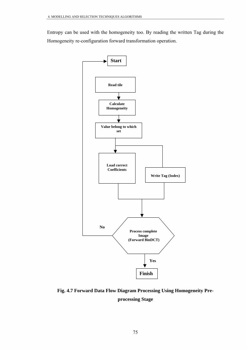
4. MODELLING AND SELECTION TECHNIQUES ALGORITHMS
Entropy can be used with the homogeneity too. By reading the written Tag during the
Homogeneity re-configuration forward transformation operation.
Fig. 4.7 Forward Data Flow Diagram Processing Using Homogeneity Pre-
processing Stage
No
Start
Read tile
Calculate Homogeneity
Value belong to which set
Write Tag (Index)
Load correct Coefficients
Finish
Process complete
Image (Forward BinDCT)
Yes
75

4. MODELLING AND SELECTION TECHNIQUES ALGORITHMS
The same twenty still images used to prod
the homogeneity database system as shown in Table 4.8. The produced single
gain across all
uration as shown in Fig. 4.9.
different homogeneity values will be then used as a database in the
ingly.
uce the entropy database is used to produce
homogeneity value for each particular configuration will be averaged a
images to get more accurate approximation to cover wider variation of the homogeneity
value that could appear. Averaging between the neighbouring points in Fig. 4.8 helps in
creating two limits or sets for each config
The calculated nine
system as set of boundaries or threshholding points. As have been done with the
entropy, the homogeneity value will be compared against the calculated thresholds
checking points and activates one of the BinDCT configurations accord
Table 4.8 Homogeneity Values Results From Processing 20 Images For Nine
BinDCT Configurations
76

4. MODELLING AND SELECTION TECHNIQUES ALGORITHMS
Fig. 4.8 Homogeneity Average For 20 Tested Images
Fig. 4.9 The New Calculated Average When Average Between Neighboured Points
77

4. MODELLING AND SELECTION TECHNIQUES ALGORITHMS
4.4 Experimental Work On Entropy Selection Technique: The proposed techniques have been tested in few images using the C custom
development programming language to emphasise and verify functionality of the
thm tested using the standard image processing Lena image. The
ntropy selection mechanism applied during the run time to configure the dynamic
proposed Entropy selection techniques.
4.4.1 Lena image
The proposed algori
e
BinDCT processor produces the following tile numbered Lena Image.
Table 4.9 Software C Code Simulation Results When Entropy Pre-processing
Stage Operates On Lena Image
This table is 32×32 cells and referred to the number of tiles in 256×256 Lena image
size. Each number in the table represents 8×8 pixels in the original raw image. The
arrows on the table shows the direction of the tile operation during the image
transformation operation. The table clearly shows that the proposed switching technique
is successfully updated at tile based. Each single number shown here is one of the
BinDCT algorithms that processed this particular tile of the image. The reconstruction
78

4. MODELLING AND SELECTION TECHNIQUES ALGORITHMS
errors for complete Lena image when processed by each configuration independently
and then reconstructed by the particular inverse configuration are shown in Table 4.10.
The error result of reconstructed the same Lena image using the entropy selection
technique and Dynamic BinDCT is also shown in same table .
Transform algorithm Without quantization image (RMSE)
With quantization (RMSE)
InvBinDCT1 0 3.733122 InvBinDCT2 0 3.725395 InvBinDCT3 0 3.748544 InvBinDCT4 0 742401 3.InvBinDCT5 0 3.741574 InvBinDCT6 0 3.744816 InvBinDCT7 0 3.811947 InvBinDCT8 0 4.022153 InvBinDCT9 0 4.395765
Re-configure Entropy 0 3.768909
Table 4.10 Reconstruction RMSE For Lena Image With Entropy Technique
RMSE between each pixel in the original and the reconstructed image is shown in Table
4.10. Not quantized Lena image when the tiles pre-processed by entropy selection
technique is reconstructed perfectly as well as when the image tiles processed by each
individual static BinDCT configurations. Fig. 4.10 (b) shows the zero difference
between the original and the reconstructed Lena image shown in Fig 4.10 (a). Entropy
selection techniqu rations.
e was used in both forward and inverse BinDCT ope
(a) (b)
Fig. 4.10 Reconstructed Lena Image Processed With Entropy Selection Technique
79

4. MODELLING AND SELECTION TECHNIQUES ALGORITHMS
The effect of the quantization step for the lossy compression is also investigated and
e most accurate BinDCT type, and BinDCT configuration 9 least
ccurate BinDCT Type is shown in Fig. 4.11 (a) and Fig. 4.12 (a). The difference
between original Lena image and the r constructed using configuration 1 and
co e
difference between origin ructed using the entropy
selecting method with generic BinDCT processor is shown to the right side of Fig. 4.13
ion 9 differences. The reconstructed image in all cases visually can not be
disti e- ig
included in Table 4.10. The standard quantization table used after the forward
transformation stage and before the inverse transformation stage was shown in Table
3.6 of section 3.5.3.
When applying the quantization step the loss of data is inevitable. The result of the
investigation carried out on processing Lena image using all static BinDCT
configurations as well as with the entropy selection-based technique with the generic
BinDCT processor is also shown in Table 4.10.
The RMSE resulted reconstructed quantized image when using BinDCT configuration 1
which is considered th
a
e
nfiguration 9 is shown to the right side of Fig. 4.11 (b) and Fig. 4.12 (b). Th
al Lena image and the reconst
(b). Entropy selection method has lower reconstruction error than using the least
approximation case. Some feature details of the image can be observed when comparing
both the reconstructed Re-configurable difference and the reconstructed using
configurat
nguished including the r configurable image shown in F . 4.13 (a).
80

4. MODELLING AND SELECTION TECHNIQUES ALGORITHMS
(a) (b)
Fig. 4.11 Reconstructed Lena Image Processed With BinDCT-C1
(a) (b)
Fig. 4.12 Reconstructed Lena Image Processed With BinDCT-C9
(a) (b)
Fig. 4.13 Reconstructed Lena Image Processed With Entropy Selection Technique
81

4. MODELLING AND SELECTION TECHNIQUES ALGORITHMS
4.4.2 Repeated Constant Tiles Image
This artificial computer-generated image shown in Fig. 4.14(a) is built to test the
functional performance of the selection methods when the whole image tiles are
constant. In this image each tile has the same pixel values. Hence each tile is different
from its neighbours. This tests the ability of the proposed technique to reconfigure on
tile based and verify the operation of matching between the expected results and
generated output results. According to the literature the constant tile under test should
always use the BinDCT configuration number 9. From the entropy point of view, the
constant tiles have zero entropy since the amount of information contained within the
tile is similar and so no data variation included in the tile. The result of this operation
match the expectation and configuration type used to process each tile in the image is
shown in Table 4.11.
Table 4.11 Software C Code Simulation Results When Entropy Pre-processing
Stage Operates On Tile Image
The RMSE result from reconstructing the repeated constant Tile image for all
configurations and using the re-configurable approach is listed in Table 4.12. The result
82

4. MODELLING AND SELECTION TECHNIQUES ALGORITHMS
shows zero reconstruction error in both tests with and without quantization step
included.
Transform algorithm Without quantization image With quantization
In 0vBinDCT1 0 InvBinDCT2 0 0 InvBinDCT3 0 0 InvBinDCT4 0 0 InvBinDCT5 0 0 InvBinDCT6 0 0 InvBinDCT7 0 0 InvBinDCT8 0 0 InvBinDCT9 0 0
Re-configure Entropy 0 0
Table 4.12 Reconstruction RMSE For Tile Image With Entropy Technique
The zero difference in reconstruction of the Re-configurable approach can be seen in
Fig. 4.13(b). The ou s test can be investigated further to emphasise and proof
the fact that the c or lossless image
c
confidential and medical sectors advantages gain in storage or
transmission time when using lossy over lossless image compression techniques.
tcome of thi
onstant images or part of the image can use lossy
ompression techniques without any loss of data. In which a vast majority of
can benefit from the
Fig. 4.14 Reconstructed Tile Im Entropy Selection Technique
(a) (b)
age Processed With
83

4. MODELLING AND SELECTION TECHNIQUES ALGORITHMS
4.5 Experimental Work On Homogeneity Selection Technique The same images used in Entropy investigation also used using the C programming
language to emphasise and verify the proposed Homogeneity selection technique.
4.5.1 Lena image
The homogeneity selection mechanism applied during the run time to re-configure the
dynamic BinDCT processor produce the following tile numbered Lena image as shown
in Table 4.13.
Table 4.13 Software C Code Simulation Results When Homogeneity Pre-
processing Stage Operates On Lena Image
The outcome of this stage proofs the ability of the proposed system to reconfigure
during run time using the Homogeneity selection method. It can be seen that different
configuration works on different tiles in the image.
84

4. MODELLING AND SELECTION TECHNIQUES ALGORITHMS
The RMSE result of reconstructing the Lena image using the re-configurable approach
as well as BinDCT-C1 and C-9 is listed in Table 4.14. The result shows zero
reconstruction error without quantization step. The reconstructed image in Fig. 4.15(a)
and the difference between the original and reconstructed image respectively shown in
Fig. 4.15(b) . The effect of the quantization on the image can be shown in Fig. 4.16.
Visual inspection for the reconstructed image cannot again distinguish the original
image from the reconstructed. Homogeneity selection method has lower reconstruction
error than using the BinDCT least approximation type configuration C9.
) (RMSE)
Transform algorithm Without quantization image
(RMSE
With quantization
Re-configure Homogeneity
0 3.800126
InvBinDCT1 0 3.733122 InvBinDCT9 0 4.395765
Table 4.14 Reconstruction RMSE Lena Image With Homogeneity Technique
(a) (b)
ot Quantized Image Processed With Homogeneity Fig. 4.15 Reconstructed Lena N
Selection Technique
85

4. MODELLING AND SELECTION TECHNIQUES ALGORITHMS
(a) (b)
Fig. 4.16 Reconstructed Lena Quantized Image Processed With Homogeneity
4.5.2 Vegi Image
selection mechanism applied to re-configure the dynamic BinDCT
Selection Technique
The Homogeneity
processor during forward and inverse transformation of the Vegi image is shown in
Table 4.15. The RMSE results from reconstructing this image also shown in Table 4.16.
The difference between the original Vegi image and the reconstructed using the
Homogeneity selecting method is shown in Fig. 4.17(b). Again we observe that the
Homogeneity selection method has lower reconstruction error than using the least
accurate BinDCT type 9. The difference between the original Vegi image and the
reconstructed using configuration type 1 and configuration type 9 is shown in Fig. 4.18
and Fig. 4.19.
86

4. MODELLING AND SELECTION TECHNIQUES ALGORITHMS
Table 4.15 Software C Code Simulation Results When Homogeneity Pre-
processing Stage Operates on Vegi Image
Table 4.16 Reconstruction RMSE For Vegi Image With Homogeneity Technique
Transform algorithm Without quantization image (RMSE)
With quantization (RMSE)
InvBinDCT1 0 2.027874 InvBinDCT2 0 2.032040 InvBinDCT3 0 2.054963 InvBinDCT4 0 2.058236 InvBinDCT5 0 2.048197 InvBinDCT6 0 2.063204 InvBinDCT7 0 2.159317 InvBinDCT8 0 2.628786 InvBinDCT9 0 3.255630
Re-configure Homogeneity 0 2.172776
87

4. MODELLING AND SELECTION TECHNIQUES ALGORITHMS
(a) (b)
Fig. 4.17 Reconstructed Vegi Image Processed With Homogeneity Selection
Technique
Fig. 4.18 Reconstructed Vegi Image Processed With BinDCT-C1
constructed Lena Image Processed With BinDCT-C9
Fig. 4.19 Re
88

4. MODELLING AND SELECTION TECHNIQUES ALGORITHMS
4.5.3 Repeated Constant Tiles
Again we use this computer-generated image to test the performance of the
homogeneity selection method. Similar to the entropy, the result of this operation match
the expectation for which configuration shall be use to process each tile. The
reconstructed image and the difference between the original image and the
reconstructed image is shown in Fig. 4.20 (a) (b) respectively . The zero difference is
obtained when operate on both quantized and not quantized data.
(a) (b)
Fig. 4.20 Reconstructed Tile Image Processed With Homogeneity Selection
Technique
4.6 Summary In this chapter, a novel detection system was proposed. The system also mathematically
modelled and investigated the relationship between different components of the design.
Detail investigation for operational procedures of the different parts of the system was
critically carried out. The two major based-selection techniques proposed here were the
Entropy and the Homogeneity. With the aid of diagrams the data flow of the operational
procedures and constructing database and threshold points for both systems were
presented. Both techniques operational outcomes were fully tested and applied on
different images. The results are tabulated and discussed through aid of different graphs.
89

4. MODELLING AND SELECTION TECHNIQUES ALGORITHMS
The outcomes of this chapter can be pointed as:
1- Very good quality for reconstructed images was obtained. RMSE results from
reconstructing the image using Entropy based-selection technique is always
lower than using Homogeneity selection-based techniques for lossy image
compression, and the same for lossless image compression as shown in Table
4.17.
Quantized image Re-configure Homogeneity (RMSE)
Re-configure Entropy (RMSE)
Lena image 3.800126 3.768909 Repeated constant
tiles 0 0
Vegi image 2.172776 2.142525 Not quantized image Re-configure Homogeneity
(RMSE) Re-configure Entropy
(RMSE) Lena image 0 0
Repeated constant tiles
0 0
Vegi image 0 0
een Results of The TwTable 4.17 Comparison Betw o Proposed Selection
description language( VHDL ).
Techniques
Having proofing the proposed selection techniques using C programming language, the
next chapter will details the hardware description of the proposed selection technique,
full details of the Entropy selection-based mechanism will be implemented and tested
using the hardware
90

5. ENTROPY SELECTION HARDWARE DESIGN
Chapter 5
ENTROPY SELECTION HARDWARE DESIGN
________________________________________________________
plementation of the proposed novel Entropy selection based technique is
vestigated further from hardware prospective using VHDL in this chapter. The
etailed C programming based investigation was introduced in chapter 4. The functional
ehaviour of the Entropy selection technique implemented in VHDL and the sub-blocks
f each module involved in this design are investigated. The hardware components
voked by the tools are also detailed.
he acronym VHDL is standing for Very High Speed Hardware Description Language.
n increasingly popular language commonly used to express complex digital design
oncepts for both simulation and synthesis. The primary intent for inventing this
nguage was to develop technologies that would permit integrated circuit to be
fabricated at or below 1 µm dimension. VHDL is a programming language widely used
to
project was Xilinx ISE9.1i [61].
The translation of the behaviour description into actual working hardware using this
language is much faster and less error prone. Various features of VHDL used during
this project were:
1- Design entry.
2- Simulation modelling.
3- Verification.
4- Netlist generator.
5.1 Introduction The im
in
d
b
o
in
T
A
c
la
describe the behaviour of any digital systems. The VHDL editor used during this
5.2 VHDL Features
91

5
. ENTROPY SELECTION HARDWARE DESIGN
92
5.2.1 VHDL as a Simulation Modelling Tool
VHDL has inherited many features appropriate for describing the behaviour of digital
electronics components from basic logic gates such as AND gate to a complete
microprocessors and ASIC designed chip. VHDL allows the functional description of
the block operation to be used; much other circuit behaviour can be modelled such as
delays through the gates and the rise or fall time of the signals. Schematic design allows
the sub-blocks of large circuits to build and simulate a complete working circuit.
5.2.2 VHDL as Design Entry Tool
VHDL as high programming language allows complex circuit design to be represented
as a computer program. Thus, it allows the behaviour of complex digital circuits to be
captured into a design system for automatic circuit synthesis or for simulation. The most
effective feature of VHDL is its ability for executing the processes in concurrent mode
not in sequential mode as rest of the computer programming languages.
5.2.3 VHDL as Netlist Generator Tool
Synthesising a design using VHDL in a computer-based environment involving
transferring the high level circuit design into low level circuit by producing the basic
gates primitives required to construct the circuit. The produced gate level circuit from
the behaviour description is then use to build the actual chip.
5.2.4 VHDL as Verification Tool
The most important application of VHDL is to capture the performance specification for
a circuit. The functional description of the circuit can be verified over the time using test
benches. One of the most useful features of VHDL is its capability to be used in the
design of test benches that produce the required signals to stimulate the system under
test. These circuit stimuli are an integral part of any VHDL project and should be
created at the same time with the description of the circuit. For real-time image
processing, applications usually work in a pipeline form. Therefore these applications
require a constant flow of input data at their input ports and generate a constant flow of
data at their output ports as shown in Fig. 5.1 for the Entropy selection technique. The
simulator used to simulate this circuit was Model Sim from Model Technology [62].

5. ENTROPY SELECTION HARDWARE DESIGN
93
Fig. 5.1 Selection Technique Test Bench Structure
5.3 Selectionata flow diagram in h
on technique design nected rd DCT processor, all
sub-modules of the design are pipelined as shown in Fig. 5.3, from which each stage
vance before th ata bec le ious stage. The
pipelining improves the throughput of the circuit and synchronise the operation between
ferent stages sh in Fig.
incoming tile to interm ory array (FIFO)
m le
he GL odule
4- Log function module (using CORDIC algorith
5- Output stage index module.
Technique Sub-Blocks The d Fig. 5.2 s ows the different stages of the entropy based-
selecti con to the forwa Dynamic Bin
cannot ad e d ome availab from the prev
different blocks.
The five dif own 5.2 are:
1- Save the ediate mem
2- GLCM Calculator odu
3- Normalising t CM m
ms)
Selection Technique.vhd
Selection_Technique_Test_Bench.vhd
CLK
RESETN
INDEX
DATA_IN_VALID
START_STREAM
DATA_IN XILINX CORDIC
IP CORE

5. ENTROPY SELECTION HARDWARE DESIGN
94
Fig. 5.2 Selection Technique Connected to Dynamic Forward BinDCT Structure
Index
Data_out
Data_in
Save tile 8x8/32 Save tile 8x8
Gray Level Co-occurrences Matrix(GLCM)
Normalisation Function
Log Function CORDIC Block
Index
rwFo ardDynamicBinDCT
Start
Finish
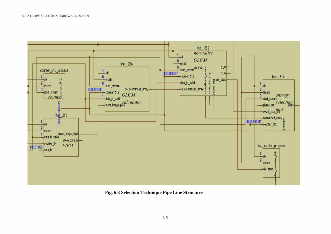
5. ENTROPY SELECTION HARDWARE DESIGN
95
calculatorGLCM
arrayGLCMnormalise
unitselectionentropycounter
FIFO
Fig. 6.3 Selection Technique Pipe Line Structure

5. ENTROPY SELECTION HARDWARE DESIGN
5.3.1 Storing The Inc
he first stage of the Entropy selection technique design is to save the incoming tile to
ted hardware block constructed by the
Figure 5.4 Save Incoming Tile Block Structure
Port
oming Tile Stage
T
an intermediate memory array. The simula
simulator to conduct the function of the FIFO to store the incoming tile is shown in Fig.
5.4. This block connected to the rest of the design blocks through an interface that
consists of a set of inputs, and output ports. The port mappings of the interface for this
block are listed in Table 5.1.
CLK
RESETN
STORE_DATA_IN
DATA_IN_VALID
STORE_IMAGE_PIXEL
COUNTER_64
DATA_IN
Direction Size Description
CLK In 1 bit signal Clock signal
RESETN In 1 bit signal Reset the block
DATA_IN_VALID In 1 bit signal Indicate the availability
of the data
DATA_IN In 8 bits bus Image samples
COUNTER_64 In 6 bits bus Control signal
STORE_IMAGE_PIXEL Out 8 bits b GLCM input array us Form
STORE_DATA_IN Out 8 bits bus Form the forward
memo
dynamic BinDCT input
ry array.
Table 5.1 S One In tage terface Port Map
96

5. ENTROPY SELECTION HARDWARE DESIGN
5.3.2 Functional description
Before constructing the hardware of the Entropy selection technique, the pixel values in
ed 2, sinc by shifting
the binary number to the right by 5 places. This shift therefore results in reducing the
value of the pixel to be in the range of 0 to 7. The maxim pixel can be
presented by 8 bits wide is 255. When shift to right 5 places is performed to a pixel
value in binary repres 255 to 7 as explain
Fig. 5.5.
his pixel value reduction was necessary to construct the GLCM for the incoming tile.
s
etermined by number of the memory locations needed to be addressed to construct 64
ifferent locations. Shifting or scaling the value down causes the pixels to lose some of
e information that it carries. Therefore another array was also constructed at the same
me with the same word length and array size of the tile. STORE_DATA_IN memory
rray is constructed to store all non-scaled pixel values to be used in later stage with
rward dynamic BinDCT block in order to perform the transformation function.
the incoming tile has to be divid by 3 e dividing 32 can be done by
um value the
re
entation, its actual value will be reduced from
in
255 in decimal = 11111111 2 in binary.
Shifting 11111111 2 by 5 to the right => 00000111 2
Fig. 5.5 Binary Shift Operation
T
Because calculating GLCM for 256 different gray scale level values of the image
requires enormous processing time and memory, hence 8 different gray scale levels is
practically sufficient.
The resultant scaled pixel value will then be saved to a memory array consists of 64
different locations functioning as FIFO, each of which has size of 8 bits wide. Thus the
output will accommodate the first tile of the image for further operation to take place.
The time needed to perform this stage will require 64 clock cycles. A 6 bits
COUNTER_64 control bus is used to index the new constructed scaled memory array
(FIFO) which called STORE_IMAGE_PIXEL. The width of the counter signal i
d
d
th
ti
a
fo
97

5. ENTROPY SELECTION HARDWARE DESIGN
Shifting the scaled pixels 5 places to the left will not result in reconstructing the same
put pixel value again. So shifting (7 => 0000011 ) to the left five places will result
(224 =>11100000 ). Hence a total loss of 31 gray scale levels may not be important
r calculating the GLCM but it’s important for performing the forward dynamic
BinDCT as well as e dynamic BinDCT
perations, and this necessitates the creation of two memory arrays in this design stage.
lis ll
. The post-fix “N” with the reset indicates that
as the data in
in 1 2
in 2
fo
for the reconstruction using the invers
o
All operations carried out inside this block were executed at the rising edge of the
control signal CLK. The block will be reset at the start of the operation to initia e a
the registers to have 0 values in all its bits
this signal is active low. After each continuous 64 DATA_IN value reads in by the input
port, the DATA_IN_VALID control signal will be negated and so it will halt first stage
block reading in any more new pixels to the system. This active high control signal will
be activated again for continuous 64 clock cycles once the output of the first tile
processing becomes ready by the forward dynamic BinDCT module block.
5.3.3 Timing Simulation
The timing simulation verifies the functional operation of this stage. The block is
presented by image pixels through its DATA_IN input port. The
STORE_IMAGE_PIXEL register files are loaded with the expected data set after
performing the division on the image samples. It will also store the nonscaled image
samples in STORE_DATA_IN register files. Fig. 5.6 shows some image pixels being
read in such as 82, 96, 97. It also shows the expected output being scaled by shifting to
the right 5 places.
82/32 = floor (2.56) = 2
96/32 = floor (3.00) = 3
97/32 = floor (3.03) = 3
The snapshot also shows the STORE_DATA_IN will be the same
samples.
98

5. ENTROPY SELECTION HARDWARE DESIGN
99
Fig. 5.6 Timing Simulation of Stage One
mory array result from stage one to next
odule will be use to construct new memory array called GLCM. The interface consists
ls and the output ports of the second stage are shown in
Fig. 5.7 Selection Technique GLCM Block Structure
5.4 GLCM Calculator Design Stage Passing the scaled STORE_IMAGE_PIXEL me
m
of the input ports, control signa
Fig. 5.7. The interface port map of this module is listed in Table 5.2.
CLK
RESETN
CO_OCURRANCES_ARRAY
DATA_IN_VALID
STORE_IMAGE_PIXEL
COUNTER_512
START_STREAM

5. ENTROPY SELECTION HARDWARE DESIGN
Port Direction Size Description
CLK In 1 bit signal Clock signal
RESETN In 1 bit signal Reset the block
DATA_IN_VALID In 1 bit signal Indicate the availability
of the data
START_STREAM In 1 bit signal Control signal
COUNTER_512 In 10 bits bus Control signal
ST
array
ORE_IMAGE_PIXEL In 8 bits bus Form GLCM input
CO_OCURRANCES_ARRAY Out 8 bits bus Form the forward
dynamic BinDCT
input array.
Table 5.2 Stage Two Interface Port Map
5.4.1 Functional Description
The scaled STORE_IMAGE_PIXEL array contains 8x8 different cell values; therefore
two nested iterati s u i a Loops invoked
for this purpose t ove e 49 iffer loca within the 64
locations. Each f n m 6 l n c x in the GLCM
array is determin fro he v e in sc ar be acc ed. The two loops
will keep track of the locations of each comb n y a remented every
time it matches. The full detail of the GLCM operation can be read in section 4.2.2.1.
The various sub-blocks of the GLCM module are shown in Fig. 5.8. If the serial
synchronise oper l rf s o l e throughput of
one memory access per cycle with different latencies. Index sub-block retrieves the
pixel from the ST E i
will be needed to odu inde
on operation were sed to access ts loc tions. Two for
o c r th d ent tions needed to be read from
or Loop is ra ge fro 0 to . The ocatio of ea h inde
ed m t alu the aled ray ing ess
inatio al gra level nd inc
ationa mode is pe ormed, each ub-bl ck wil ensur
ORE_IMAGE_PIX L reg ster files storage. A total of 10 clock cycles
pr ce xing of the two locations in the register files, the latency
100

5. ENTROPY SELECTION HARDWARE DESIGN
distributed within the index sub-blocks we
operations, and t clo cyc to l the o lo tion to t two registers Loc0
and Loc1. The fi t il r u e M s s after 13 clock
ycles. One clock cycle will be needed to shift register Loc0 followed by one clock
cycle to add both Loc registers then it will be written out to the GLCM register files.
Fig. 5.8 GLCM Internal Block Structure
nt for five addition operations, three shift
wo ck les oad tw ca s in he
nal ou put w l be w itten o t to th GLC regi ter file
c
The total number of clock cycles required to perform 8x8 register files according to
serial implementation will be (13x49=637 clock cycles). If the FPGA run at 100MHz
the total execution time required calculating the GLCM register files will be 6.37 sµ .
The serial implementation of the algorithm is the most efficient in terms of hardware
plementation. Thus, the utilized area used from the chip is small. The hardware
nsists of 6 addition circuits, three shift
he execution time can be done over the area using the concepts of
r Loops. There are two different types of for Loops, rolled and unrolled for Loops.
olled for Loop adopt the serial synchronise operational mode, in which one iteration of
e loop will be executed each clock cycle. Thus 49 clock cycles will be needed to
onstruct the GLCM array. According to rolled for Loop concepts the 13 clock cycles
im
blocks needed to perform Fig. 5.8 then co
registers and two blocks of memory arrays containing 64 register files for
STORE_IMAGE_PIXEL and a 64 register files to construct the GLCM.
More utilization for t
fo
R
th
c
Index
STORE_IMAGE_PIXEL
Loc1
Loc0 Shift Loc0
+
GLCM
101

5. ENTROPY SELECTION HARDWARE DESIGN
required by the serial implementation of the GLCM block become 1 clock cycle and
erefore the hardware primitives used to work in parallel and to construct the GLCM
ill required more registers to hold the values of the intermediate results from each sub-
lock.
he hardware invoked to calculate the GLCM according to the rolled for loop was:
counter 10 bits wide.
register of 6 bits wide
register of 8 bits wide.
26 register files of 6 bits wide for two STORE_IMAGE_PIXEL
98 regist
he unrolled for loop works in parallel operational mode, in which the system will do
-copy of the for Loop hardware circuit 49 different times to achieve operational
lism. The advantage of the unrolled fo t the wh ons of the
an be done in 1 clock c . The h ng and p using
increases the a used by therefo icient
rawback of operati at it wil r area of
the chip designated for the design. The hardware components needed to construct this
ll i
hich the hardware invoke be:
nter 10 bits wide.
43 register of 8 bits wide.
6272 register files of
136 register files of 6 bits wide for the GLCM_TEMP.
or the GLCM.
_OCURRANCES_ARRAY) becomes ready after 65 clock
cycles as indicated by COUNTER_512.
th
w
b
T
1
6
7
1
er files of 6 bits wide for the two GLCM
T
multi
paralle r Loop is tha ole 49 iterati
for Loop c ycle uge time savi rocessing speed
this method have rea the design, re create less eff
area utilization. The d this on mode is th l occupy large
new circuit will duplicate the ro ed for Loop circuit 49 different t me.
From w d will
49 cou
294 register of 6 bits wide
3
6 bits wide for two STORE_IMAGE_PIXEL
3
64 register files of 6 bits wide f
5.4.2 Timing Simulation Test
GLCM functional block was tested from within the complete deign using Lena image.
The snapshot waves in Fig. 5.9 shows a tile was read in from the previous stage
STORE_IMAGE_PIXEL and processed by the GLCM module and being written out.
The GLCM registers file (CO
102

5. ENTROPY SELECTION HARDWARE DESIGN
GLCM register files contain the number of occurrences for each possible grey level
combination within the STORE_IMAGE PIXEL register files. The combination of grey
levels (2, 2) from Fig. 5.9 has occurred 6 times. The combination of grey levels (3, 2)
has occurred 12 times. The combination of grey levels (4, 2) has occurred 1 time. The
combination of grey levels (2, 3) has occurred 2 times. The combination of grey levels
(3, 3) has occurred 22 times. The combination of grey levels (4, 3) has occurred 5 times.
Fig. 5.9 Simulation of Stage Two
3 3 2 3 2 3
3 3 3 2 3
2 2 3 2 3 4
2
3
3
3
3
3
4
2
3
3
3
3
3
4
2 3 3 3 3 3 3 4
2 3 3 3 3 3 3 4
3 3 3 3 3 3 3 4
2
2
2
2
2
2
2
2
2
103

5. ENTROPY SELECTION HARDWARE DESIGN
Table 5.3 The Calculation of The GLCM For STORE_IMAGE_PIXEL Grey
Levels (2, 2)
The total number of occurrences for all possible grey level combinations therefore
grey levels (2,
2) is shown in details in Table 5.3. The number of occurrences for a specific grey level
th ociated with it. Th whole GLCM table
r this particular tile is shown in Table 5.4.
becomes 49. The calculation of the GLCM for STORE_IMAGE_PIXEL
can be count from e number of the arrows ass e
fo
0
(0.0)
0
(0.1)
0
(0.2)
0
(0.3)
0
(0.4)
0
(0.5)
0
(0.6)
0
(0.7)
0
(1.0)
0
(1.1)
0
(1.2)
0
(1.3)
0
(1.4)
0
(1.5)
0
(1.6)
0
(1.7)
0 0 6 12 1 0
(2.0) (2.1) (2.2) (2.3) (2.4) (2.5)
0
(2.6)
0
(2.7)
0 0
(3.0) (3.1)
0 0
(3.6)
0
(3.7)
3 22 5
(3.2) (3.3) (3.4) (3.5)
0
(4.0)
0
(4.1) (4.4) (4.5) (4.6) (4.7)
0 0 0 0 0 0
(4.2) (4.3)
0
(5.0)
0
(5.1) (5.2) (5.3) (5.4) (5.5)
0
(5.6)
0
(5.7)
0 0 0 0
0
(6.0)
0
(6.1) ) (6.4) (6.5) (6.6) (6.7)
0 0 0 0 0 0
(6.2) (6.3
0
(7.0)
0
(7.1)
0 0 0 0 0 0
(7.2) (7.3) (7.4) (7.5) (7.6) (7.7)
Table 5.4 The Whole GLCM Table For This Particular Tile
Based on the hardware desi cision
needs to be taken whether to ution time.
general the chnology is ways moving faster, so the number of gates available to
t any s get ring
gn specification and the technology available a de
go for less utilized chip size or faster exec
In te al
implemen design i ting bigger, this caused by the successful manufactu
104

5. ENTROPY SELECTION HARDWARE DESIGN
logic gates and with nology and is continue to get
Since the technology is movi been chosen over
the size. Although the size of the current chip cannot fit the whole design when adapt
unrolled for Loop operational mode. Limitations within the Virtex architecture
development tools, and the testability and hardware configuration were exposed.
START_STREAM control signal indicates the start of reading new tile in. This control
signal reset counter_512 after 293 clock cycles which can be represented in 10 bits. The
293 comes from calculating the total number of clock cycles to process each tile from
read e las ension of the
rward dynam c BinDCT operation. GLCM calculation will be executed when
R_51 l to 6
rm he Gulati LCM egister file. The entropy selection technique proceeds to
the G ray. T n consisting from the
input ports, con rol signals an rt map
listed in Table 5.5.
Fig. 5.10 Selection Technique Normalised GLCM Block Structure
IC chips reduce sizes up to 60 nm tech
smaller.
ng forward, for this project a speed had
first pixel until th t output coming out from the second dim
fo i
COUNTE 2 is equa 5.
5.5 No alising t LCM Stage Upon calc ng the G r
normalise LCM ar he interface of the normalise functio
t d the output ports are shown in Fig. 5.10 and the po
NORMALISED_ARRAY
NORM_FUN_RDY
X_IN
Y_IN
COUNTER-512
CLK
RESETN
DATA_IN_VALID
CO_OCURRANCES_ARRAY
105

5. ENTROPY SELECTION HARDWARE DESIGN
Description
Port Direction Size
CLK Clk signal In 1 bit signal
RESETN In 1 bit signal Reset the block
COUNTER_512 Control signal In 10 bits bus
DATA_IN_VA
of the data
LID In 1 bit signal Availability
CO_OCURRA RRA In Array of 6 bits bus GLCM input arrayNCES_A Y
NORM_FUN_ DY R Out 1 bit signal Control signal
X_IN Out 8 bits bus Input for CORDIC
Y_IN Out 8 bits bus Input for CORDIC
NORMALISED Y Output array _ARRA Out Array of 6 bits
Table 5.5 Stage Three Interface Port Map
ction iption
M r ique to works.
sation rts by reading in and sums all the values of the GLCM register
le through cyclic loop operation. The computed sum register will be used as the
divisor of the nex be divided by the
ing point number. When
resenting a number using fix point notation, the responsibility for keeping track of
5.5.1 Fun al Descr
eeds to be normalised for this technThe GLC
Normali
egister file n
stage sta
fi
t step. Each individual GLCM value (dividend) will
sum (divisor) calculated previously, thus the main operations to be carried out in this
stage is the binary division.
To increase the execution rate or to improve throughput calculations of the algorithm,
the fixed point presentation will be used to represent the float
rep
and determine the position of the virtual point place is the responsibility of the
programmer. The labelling standard for unsigned fixed point notation is given in Eq.
(5.1):
Q[QI].[QF] (5.1)
106

5. ENTROPY SELECTION HARDWARE DESIGN
Where QI = number of bits representing integer part of the notation.
QF= number of bits representing fractional part of the notation.
umber consists of the sum of
) and (QF). This sum is commonly referred to as Word
Q8.8 would be a 16 bit value with 8 bits to represent the
nt the fractional part.
e carried out using a shift
procedures shown
11 . The results of
The total number of bits used to represent any fix point n
number of both bits of (QI
Length (WL). From Eq. (5.1),
integer part and 8 bits to represe
5.5.1.1 Division Algorithm
Division of numbers represented in fixed point notation can b
and subtract approach similar to decimal numbers long division. The
in Table 5.6 divided a dividend of 0000001 2 by the divisor of 00011 2
dividing 151 is equal to 0.066 in decimal representation, and in signed binary its given
by divisor
dividend = 2
2
00011110000001 .
The normalisation functions will always have dividend less than divisor. Therefore, 6
bits will be added in front of the number to account for the fractional values below the
decimal point, hence creating the fix point presentation. To get more accurate results the
wer six bits of the number that below the decimal point has to be increased, which
in the utilised FPGA chip, so 6 bits shall give a close
000101.11000 => 5.75
According to this
lo
will result in using more area
approximation for the value under the decimal point. The same procedures can be
conducted when the dividend is bigger than the divisor, in this case 6 bits of zero values
will be added to the back end of the number and hence ignored, the rest of the operation
procedures are still the same. If we have a number in a register 000101110000 2 this
could be read according to fixed point as
Integer Fraction
0 2
151 now will be converted to
2
2
000000.0001111000000.0000001
107

5. ENTROPY SELECTION HARDWARE DESIGN
The flow of the division algorithm data starts by registering the dividend and initialise
the register by shifting it one bit to the left. The algorithm then keeps subtract the
divisor from the dividend if the value of the dividend is bigger. After the subtraction
operation done the results will then be shifted one bit to the left. The data flow will keep
repeating the same previous operations until all 6 fractional bits is shifted. The results
then will be the reminder and the quotient will be ignored.
Integer Fraction Main Operation
0000001 000000 (a) Load dividend register
0000010 00000 ft it one bit to the
Left.
0 (b) Initialise dividend register by shi
0000010
-
0001111
0000010
0000100
0000100
000000
000000
000000
00000x
000000
(b) Subtract divisor form dividend if dividend is
bigger.
(c) Store the result in dividend register otherwise keep
the register unchanged.
(a) Keep dividend register.
(d) Shifted one position to the left.
(e) MSB of dividend register filled by 0 because
subtracts operation not executed.
0000100
001111
-
0
0000100
1000
000000
000000
0001000
000
000000
00000x
000000
(a) Keep devisor register.
(b) Subtract divisor form divisor if divisor bigger.
(c) Store the result in dividend register otherwise keep
the register unchanged.
(d) Shifted one position to the left.
(e) MSB of dividend register filled by 0 because
subtracts operation not executed.
108

5. ENTROPY SELECTION HARDWARE DESIGN
0001000
-
001111 0
0001000
0010000
0010000
000000
000000
(c)
000000
00000x
000000
the register unchanged
(d) Shifted one position to the left.
(e) MSB of dividend register filled by 0 because
subtracts operation not executed.
(a) Keep devisor register.
(b) Subtract divisor form divisor if divisor bigger.
Store the result in dividend register otherwise keep
0010000
-
0001111
0000001
0000010
0000010
000000
000000
000000
00000x
000001
(c) Store the result in dividend register otherwise keep
the register unchanged.
(d) Shifted one position to the left.
(e) MSB of dividend register filled by 1 because
subtracts operation executed.
(a) Keep dividend register.
(b) Subtract divisor form divisor if divisor bigger.
0000010
-
0001111
000
000
000
000001
0010
0100
0100
000000
(b) Su
000001
00001x (c
000010 the register unchanged.
(a) Result from subtraction loaded to dividend
register.
btract divisor form divisor if dividend bigger.
) Store the result in dividend register otherwise keep
oison to the left.
(d) Shifted one p
(e) MSB of dividend register filled by 0 because
subtract operation not executed.
0000100 000010 (a) Result from subtract
-
ion loaded to dividend
register.
109

5. ENTROPY SELECTION HARDWARE DESIGN
00 10111
000100 0
0001000
0001000
000000
000010
(b) Subtract divisor form divisor if dividend bigger.
(c) Store the result in dividend register otherwise keep
00010x
000100
the register unchanged.
(d) Shifted one poison to the left.
(e) MSB of dividend register filled by 0 because
subtracts operation not executed.
xxxxxxx
quotient
ignore
000100
1/16 =
0.0625
Six bits reminder below the point is the best
approximation of the expected answer
Table 5.6 Division Algorithm Working Example
initialise outputting X_IN and Y_IN to form
o o oc n s st g d s
stage will contain 64 registers each of which have 6 bits wide.
The design was verified using VHDL sim or, but synthesising this design to fit the
i w e r n to m e
normalised function was too big. The unrolled for Loop hardware architecture have
een d to im ement the normalization function in two places, the first one was when
reading the GLCM and calculating the su he second was when divided the GLCM
entries by the sum. The the tools to perform the
ithin the available chip size.
d e the GLCM was:
343 comparators of 6 bits wide,
343 register of 8 bits wide,
Normalisation calculation will be executed when the COUNTER_512 is equal to 66.
NORM_FUN_RDY control signal will be ready in the same clock cycle with the
normalised register file. This signal will
the inputs f the L g functional bl k. The ormali ed regi er file enerate by thi
ulat
Virtex arch tecture as not proved becaus the ha dware eeded imple ent th
b use pl
m, t
irregular hardware structure invoked by
cyclic loop operations makes it impossible for the available chip to route the design
w
Thus, the hardware invoke to calculat
49 counter 10 bits wide,
49 register of 6 bits wide,
98 register of 11 bits wide,
110

5. ENTROPY SELECTION HARDWARE DESIGN
4096 register files of 6 bits wide GLCM to calculate the sum,
4096 register files of 6 bits wide GLCM to be read for normalisation,
096 register files of 6 bits wide NORMALISED_ARRAY_TEMP,
ulate the division
lgorithm x 64 dividend) + (64 to write the NORMALISED_ARRAY).
5.5.2 Timing Simulation Test
The NORMALISED_ARRAY register files become ready after 66 clock cycles as
U ER_512. The normalisation block will read in the GLCM first and
calculate the sum ch equal to (49) for this particular tile. Each individual GLCM
register file then will be divide by the sum and written out as NORMALISED_ARRAY.
he first value of the GLCM is 6, when divided by the sum 49 then
4
64 register files of 6 bits wide for NORMALISED_ARRAY.
By analysing the structures of the for Loop, it was concluded that the algorithm was
more suited for a multi FPGA system rather than a single FPGA based implementation
unless the rolled for Loop is used, hence the number of the clock cycles to perform this
operation will increase from 1 clock at the moment to a total of 576 clock cycles (64
clocks to calculate the divisor (sum value)) + (7 clocks to calc
a
indicated by CO NT
whi
The timing simulation of stage three is shown in Fig. 5.11. The example from the
functional simulation of the design is given below:
T
496 = 0.12210 =~ (
161 +
321 +
641 ) = ~ (0.1110 ).
This example verifies normalised value calculation operation.
The difference between the 0.12210 and when representing by fix point 0.1110 is caused
the number of bits was used to repreby sent the fractional part of the number. To get
more accuracy simply increase the width. According to Table 5.6, the norm lised value
will be represented by 6 bits below the decimal point; hence from irst
normalised value within the array was 7 which equal to 000111 . The snapshot
simulation will show 7 because keeping track the decimal point in fix point notation is
the responsibility of the program er. And hence 7 = 00.000111 in 1Q.7 format.
Thus approving that functional operation of the block is outputting the right results.
a
the snapshot the f
10 2
m 10 2
111

5. ENTROPY SELECTION HARDWARE DESIGN
Fi Tim imu on o ge T
.6 Log Function and Index Design y te e ce a c ng
M ISED RRA hen rodu X_ _IN alcu he y
alue. The first step to calculate the entropy started from calculating natural log of the
ormalised GLCM register files. The interf
he input ports, control Fig. 5.12 and the port
g. 5.11 ing S lati f Sta hree
5The entrop selection
and
chniqu
p
pro
ng
eds
, Y
fter
o c
alculati
te t
the
tropNOR AL _A Y ce ci IN t la en
v
n ace of the natural Log function consists of
t signals and the output ports as shown in
mapping listed in Table 5.7.
Fig. 5.12 Selection Technique Log Function Block Structure
PHASE_OUT
X_IN
Y_IN
CLK
RDY
112

5. ENTROPY SELECTION HARDWARE DESIGN
Port Direction Size Description
CLK In 1 bit signal Clock signal
X_IN In 8 bits bus Input for CORDIC
Y_IN RDIC In 8 bits bus Input for CO
PHASE_OUT Out 8 bits bus Output bus
RDY Out 1 bit signal Debug signal
Table 5.7 Stage Four Log Function Interface Port Map
Calculating the entropy function requires calculating the natural log of base 2.78 for the
CORDIC
gorithm was used to calculate the Log function. The COordinate
Rotation DIgital Computer algorithm is a set of shift-add algorithms and can compute
nge of functions including trigonometric, hyperbolic, square root, linear and
solve problems of the real-time navigation digital systems.
In this rese t m the log
alculations of the entropy function. A fully parallel architectural configuration with
ge of functional configurations. The
llowing functional configurations are available and can be selected using this core:
3- Arc-Tangent calculations
calculations
r ulations
5.6.1 Functional Description
each of the GLCM normalised values. The hardware efficient well-known
trigonometric al
ra
logarithmic functions [63]. The CORDIC algorithm is originated by Volder [64] and has
been developed to
arch Xilinx CORDIC IP core generator is used o perfor
c
single-cycle execution time was selected. The drawback of this architectural
configuration is the occupation for large silicon area of the available chip. The Xilinx IP
CORDIC core can be used to perform a ran
fo
1- Rotate calculations
2- Sine and Cosine calculations
4- Square Root calculations
5- Translate calculations
6- Hyperbolic Sine and Hyperbolic Cosine
7- Hyperbolic A c-Tangent calc
113

5. ENTROPY SELECTION HARDWARE DESIGN
Configuration (7) Arch-Tanh is the operation that was used with the novel Entropy
t of the following Equation 5.2 is the part
n Xilinx IP CORDIC core.
selection technique circuit design. The ln() par
targeted and implemented i
( )∑−
0, ji
ssed using signed binary numbers of 1QN
format. All data input ports are read simultaneously to form a single input sample. The
output ports, PHASE_OUT, which was expressed using signed binary numbers of 2QN
The width of the data input and
utput ports are configured using the parameter input width of the GUI provided by
ut and output ports explained in
ctions.
5.6.1.1 Input Port Calculations
Both Input data signals X_IN and Y_IN represented in 1Q7 format, as shown in Tables
ust be in the range: 1 <= input data signal <= -1. Input data outside this
) bit(2) bit(1) bit(0)
=
−=1
,,
N
jiji LnPPE (5.2)
In general, CORDIC IP core configuration 7 has three inputs ports X_IN, Y_IN, and
CLK port. The first two input ports expre
format and one bit signal RDY are shown in Fig. 5.12.
o
Xilinx to configure the core. The calculation of both inp
more details in the following se
5.8(a) and (b), m
range will produce unpredictable results.
bit(7) S bit(6) Virtual point bit(5) bit(4) bit(3
0 1 . 0 0 0 0 0 0
(a)
bit(0)
bit(7) S bit(6) Virtual point bit(5) bit(4) bit(3) bit(2) bit(1)
1 1 . 0 0 0 0 0 0
(b)
Table 5.8 Input Data Representation
In 1Q7 format values, +1 and -1 are represented as: 01000000 2 => 01.000000 2 => +1.0.
1100000 => 11.000000 => - 1.0. 0 2 2
114

5. ENTROPY SELECTION HARDWARE DESIGN
The input to this module comes from reading the GLCM normalized matrix. Each value
en will be used to form the two inputs X-IN and Y_IN at the same time. The GLCM
ormalized values are usually positive numbers between 0 and 1, and has been set to a 6
its wide. However the input to the module has 8 bits wide and so two more bits
quired to be added to the normalized value.
alculating the log function using the CORDIC is determine through calculating the
rcTanh of the two input values X_IN, Y_IN. When the ArcTanh functional
onfiguration is selected, the CORDIC algorithm is used to move the input vector
_IN,Y_IN) along the hyperbolic curve until the Y_IN component reaches zero. This
enerates the hyperbolic angle ArcTanh(Y_IN /X_IN). The hyperbolic angle represents
e Log of the area under the vector (X_IN,Y_IN) and is unrelated to a trigonometric
ngle. The relationship between the two functions is summarized by
th
n
b
re
C
A
c
(X
g
th
a
Ln( ⎥⎦
⎤⎡=
INYArcTanh _2)α (5.3) ⎢⎣ INX _
here Y_IN = W α -1,
X_IN = α +1.
ince the two input ports of the ArcTanh function (X_IN, Y_IN) can be formed from a
sin lue by adding one and g according to Eq rom
S
gle va subtractin one . (5.3) then f α the
GLCM normalised value read in can form both input ports.
However α is a positive value less tha ays with creation
of the two input ports can be simple. Th ching 0 X_IN, and
to form Y_IN does not required any adder for X_IN port or
su N port, it on required the MSB of
and n 1 and alw 6 bits wide, the
erefore atta 1 2 to form
always attaching 11 2
btractor for Y_I ly to concatenate the two bits to
α as shown in the example in F 5.13. ig.
115

5. ENTROPY SELECTION HARDWARE DESIGN
If α = 0.1110 in decimal or 00.100110 2 in 1Q7 format then
X_IN = (0.1110 +110 ) = 01.000111 2 (+110 + 0.1110 = +1.1110 ).
Y_IN = (0.1110 -110 ) = 11.000111 2 (-210 + 110 + 0.1110 )= (-0.8910 ) .
Fig. 5.13 Creating The Two Input Port From α
5.6.1.2 Output Port Calculation
The output signal PHASE_OUT is always represented in 2QN format as shown in Table
e: -4 <= output_data <= 3.984375 or (4-(1/64)). 5.9(a) and (b). The output rang
bit(8) Bit(7) bit(6) S
Virtual point
bit(5) 1/2
bit(4) 1/4
bit(3) 1/8
bit(2) 1/16
bit(1) 1/32
bit(0) 1/64
0 1 1 . 1 1 1 1 1 1
(a) bit(8)
Bit(7) bit(6) Virtual
pbit(5) bit(4) bit(3) bit(2) bit(1)
bit(0) 1/64 S oint 1/2 1/4 1/8 1/16 1/32
1 0 0 . 0 0 0 0 0 0
(b)
ln(
Table 5.9 Output Data Representation
Since the output of the CORDIC block is the natural Log then According to Eq. (5.3)
PHASE_OUT will be equal to α . In 2Q7 format value PHASE_OUT value equal to
o verify the functional simulation of the normalisation block, the snapshot taken shows
+3.25, -3.25 are represented as:
011010000 2 => 011.010000 2 => (+3 + 0.25) => +3.25
100110000 2 => 100.110000 2 => (- 4 + 0.75) => -3.25
5.6.2 Timing Simulation Test
T
the first value read from NORMALISED_ARRAY which was α = 0.1110 . This value is
equal to 000111 2 below the virtual decimal point. For Xilinx CORDIC IP core both
116
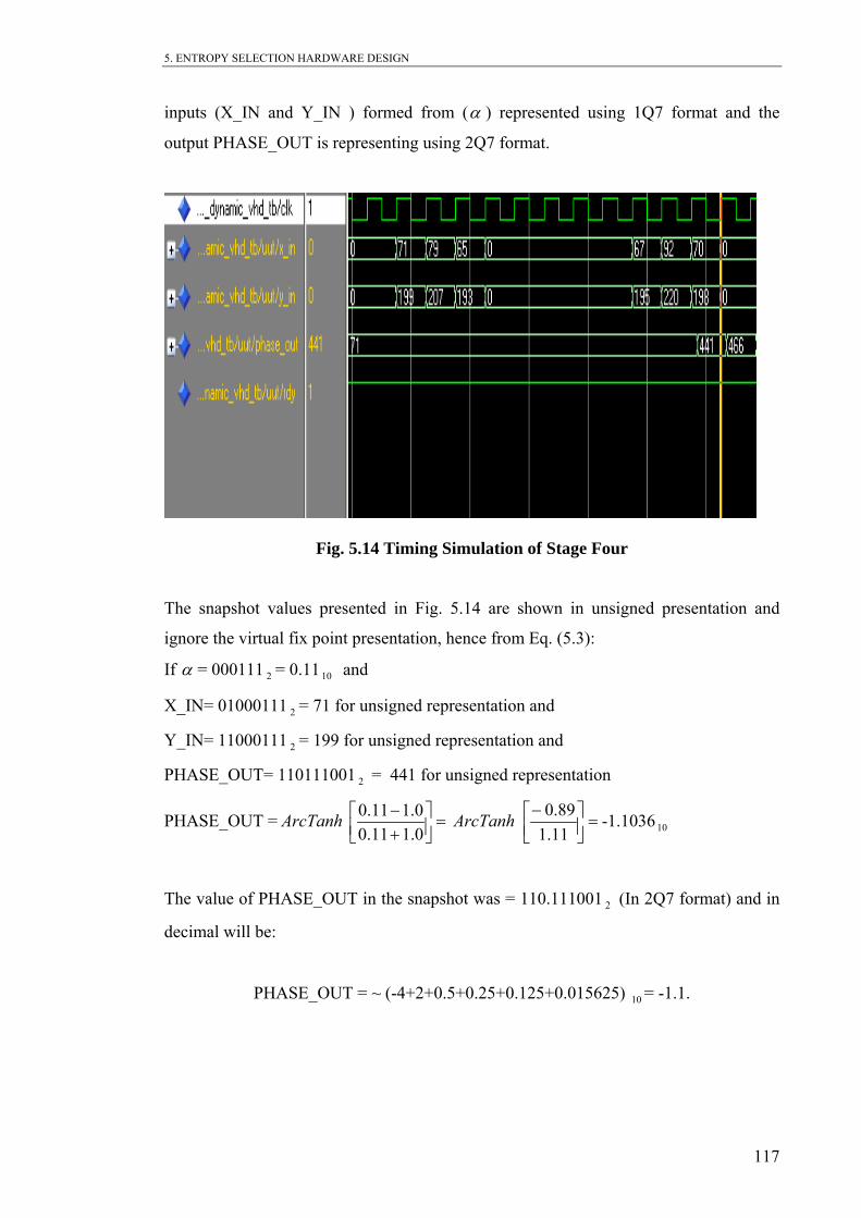
5. ENTROPY SELECTION HARDWARE DESIGN
inputs (X_IN and Y_IN ) formed from (α ) represented using 1Q7 format and the
output PHASE_OUT is representing using 2Q7 format.
Fig. 5.14 Timing Simulation of Stage Four
The snapshot values presented in Fig. 5.14 are shown in unsigned presentation and
ignore the virtual fix point presentation, hence from Eq. (5.3):
If α = 000111 = 0.11 and
X_IN= 01000111 = 71 for unsigned representation and
Y_IN= 11000111 = 199 for unsigned representation and
PHASE_OUT= 110111001 = 441 for unsigned representation
PHASE_OUT =
2 10
2
2
2
=⎥⎦⎤
⎢⎣⎡
+−
0.111.00.111.0ArcTanh =⎥⎦
⎤⎢⎣⎡−
11.189.0ArcTanh -1.1036
The value of PHASE_OUT in the snapshot was = 110.111001 (In 2Q7 format) and in
decimal will be:
PHASE_OUT = ~ (-4+2+0.5+0.25+0.125+0.015625) = -1.1.
10
2
10
117

5. ENTROPY SELECTION HARDWARE DESIGN
The result obtain calculating Ln(0.11) by calculator match the value calculated by the
i esign. Another way of verifying the Ln(0.11) function
= 71
=199
=441
X_IN = 01000111
X_IN = (+)1.000111 (in 1Q7 format)
X_IN = 1.11 (in decimal )
CORDIC IP core used in th s d
based on the snapshot simulation as following:
X_IN = 01000111 2
Y_IN = 11000111 2
PHASE_OUT= 110111001 2
The input X_IN can be calculated as follows:
2
2
10
The input Y_IN can be calculated as follows:
_IN = 11000111
_IN = (-) 1.000111
Y 2
Y 2(in 1Q7 format)
pply 2’s complement to the Y_IN since its negative number by invert the bits and add
to the result
_IN = 1.000111
A
1
Y 2 ignore the sign bit for now
_IN = 0.111000(invert the bits)
_IN = 0.111001(add 1)
_IN = 0.890625 (in decimal)
_IN = - 0.89062 (Remembering the sign)
Y
Y
Y 10
Y 510
he output PHASE_OUT can be calculated as follows:
Apply 2’s complement to the PHASE_OUT since its negative number by invert the bits
and add 1 to the result:
PHASE_OUT = 01.000110(Ignoring the sign bit for now)
T
PHASE_OUT = 110111001 2
PHASE_OUT = 110.111001 2
PHASE_OUT = (-) 10.111001 2
118

5. ENTROPY SELECTION HARDWARE DESIGN
PHASE_OUT = 01.000111(Add 1)
PHASE_OUT = 1.11 (Value in decimal)
PHASE_OUT ( h
5.7 Index The last step of the final stage to construct the Entropy selection technique was to
output the index. The index calculation m diately after obtaining the
PHASE_OUT for all the tile array m mbers in the process. The interface of the index
function consists of the input ports, control signals and the output ports as shown in Fig.
5.15 and the port ma isted Table .10.
Fi e d
10
= -1.1110 Remembering t e sign)
design
starts im e
e
p l in 5
g. 5.15 CORDIC IP Cor With The In ex Interface
INDEX
PHASE_OUT
COUNT_FINAL_LOG
COUNTER_512
CLK
RESETN
START_STREAM
NORMALISED_ARRAY
PHASE_OUT
X_IN
Y_IN
CLK
RDY
119

5. ENTROPY SELECTION HARDWARE DESIGN
Port Direction Size Description
CLK In 1 bit signal Clock signal
RESETN In 1 bit signal Reset the block
COUNTER_512 In 10 bits bus Control signal
START_STREAM In 1 bit signal availability
of the data
PHASE_OUT In Array of 8 bits bus Ln() value
NORMALISED_ARRAY In Array of 6 bits bus GLCM Norm. values
COUNT_FINAL_LOC In 8 bits bus Control signal
INDEX ut to BinDCTs Out 1 bit signal Outp
Table 5.10 Stage Five Index Interface Port Map
n number will be
ady after 139 clock cycles. The hardware needed to calculate the index is:
its wide
8 comparators of 10 bits wide
o be multiplied by two according to Equation 2 in section 5.6.1.2.
5.7.1 Functional Description
The configuration number required to reconfigure the forward dynamic BinDCT will
use the PHASE_OUT value and multiply it with the NORMALISED_ARRAY and sum
the results for the remaining 64 register files. The index configuratio
re
1 counter 10 bits wide
6 shift registers of 9 bits wide
6 shift registers of 8 b
1
1 register of 6 bits wide.
1 register of 10 bits wide.
64 register files of 6 bits wide for NORMALISED_ARRAY
6 addition circuits
The PHASE_OUT values are obtained in serial fashion from the CORDIC block and
have t
If α = 000111 2 = 0.1110 and PHASE_OUT = 110111001 2 =-1.1110 then
Ln( 2.211.1*2PHASE_OUT*2) 10 −=−==α 10 .
120
5. ENTROPY SELECTION HARDWARE DESIGN
To verify the output of the design, the calculator can be used to calculate the
Ln(0.11)=~-2.2 and hence both values are identical.
5.7.2 Multiplication Algorithm
Since the NORMALISED_ARRAY values needs to be multiplied by its Ln(α ) value,
therefore this multiplication in binary can be accomplished using a shift and add
approach. When multiplying two numbers, the multiplicand is added to the product
number of times the value of the multiplier. The multiplier design is constructed in
VHDL and it uses the signed operational flow procedures shown in Fig. 5.16.
The operation of this unit performs product term in each stage by one bit with respect to
the previous stage and decides whether to shift the multiplier number or not. The
direction of the shift operation is determined based on the value of the multiplicand. If
the value of the multiplicand is less than 1 then the shift will be to the right, the position
of the multiplier bits used being right shifted by one bit each successive operation. If the
multiplicand is bigger than 1 the shift will be to the left. Shifting to the left will increase
the value. The multiplicand number comes from reading the NORMALISED_ARRAY;
therefore it will always be less than 1. The partial products results from this cyclic
operation become the final product by summing up the entire partial product registers
from each sage.
In general this multiplication unit checks the multiplier number against each bit of the
multiplicand in turn. If the multiplicand bit being checked has the value of 1, a new
register will store the new version of the multiplier shifted to the right by number of bits
the1 bit is located in the multiplicand. If the bit has value of zero then the register will
be loaded by zeros. At the end the whole registers will be added together to form the
final result. When multiplying 32 by 1/16 the answer should be equal to 2, in binary,
this is represented by 100000 /0.0001002 2
121

5. ENTROPY SELECTION HARDWARE DESIGN
5. ENTROPY SELECTION HARDWARE DESIGN
122
he flow data of this operation according to the multiplication algorithm is:
Reg = Multiplier =100000 .
Multiplicand = 0.000100
Reg1 = 000000
Reg2 = 000000
. 5.16 The Operational Procedures of The Multiplier Design
T
2
2
2 .
2 .
Reg3 = 000000 2 .
Reg4 = 000010 2 .
Reg5 = 000000 2 .
Reg6 = 000000 2 .
Result = Reg1+ Reg2+ Reg3+ Reg4+ Reg5+ Reg6 = 000010 2
Fig
After all NORMALISED_ARRAY values being multiplied by their Ln(α ) values.
They will be summed and therefore producing the entropy value. The calculated
entropy for each tile is expressed in the fixed point 2Q8 format. The fractional portion
of the entropy boundaries is approximated to the nearest value and listed in Table 5.11.
Result
Reg1
Reg2
Reg3
Reg4
Reg5
Reg
>>6
>>1
>>2
>>3
>>4
>>5
+
+
+
+
Reg6
122
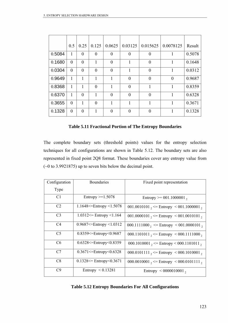
5. ENTROPY SELECTION HARDWARE DESIGN
0.5
0.25
0.125
0.0625
0.03125
0.015625
0.0078125
Result
0.5084 1 0 0 0 0 0 1 0.5078
0.1680 0 0 1 0 1 0 1 0.1648
0.0304 0 0 0 0 1 0 1 0.0312
0.9649 1 1 1 1 0 0 0 0.9687
0.8368 1 1 0 1 0 1 1 0.8359
0.6370 1 0 1 0 0 0 1 0.6328
0.3655 0 1 0 1 1 1 1 0.3671
0.1328 0 0 1 0 0 0 1 0.1328
Table 5.11 Fractional Portion of The Entropy Boundaries
The comp e tropy selection
techniques r
represented in tropy value from
(~0 to 3.99 8
let boundary sets (threshold points) values for the en
fo all configurations are shown in Table 5.12. The boundary sets are also
fixed point 2Q8 format. These boundaries cover any en
21 75) up to seven bits below the decimal point.
Configuration
Type
Boundaries Fixed point representation
C1 Entropy >=1.5078 Entropy >= 001.1000001 2
C2 1.1648<=Entropy <1.5078 001.0010101 2 <= Entropy < 001.1000001 2
C3 1.0312<= Entropy <1.164 001.0000101 2 <= Entropy < 001.0010101 2
C4 0.9687<=Entropy <1.0312 000.1111000 2 <= Entropy < 001.0000101 2
C5 0.8359<=Entropy<0.9687 000.1101011 2 <= Entropy < 000.1111000 2
C6 0.6328<=Entropy<0.8359 000.1010001 <= Entropy < 000.11010112 2
C7 0.3671<=Entropy<0.6328 000.0101111 <= Entropy < 000.10100012 2
C8 0.1328<= Entropy<0.3671 000.0010001 <= Entropy < 000.01011112 2
C9 Entropy < 0.13281 Entropy < 0000010001 2
Table 5.12 Entropy Boundaries For All Configurations
123

5. ENTROPY SELECTION HARDWARE DESIGN
5.7.3 Timing simulation test
he snapshot of this stage shown in Fig. 5.17 emphasises the success of this selection
chniques and shows its ability to calculate the entropy for each tile, and hence
pares the result with the threshold points and produces the correct BinDCT
onfiguration for each tile. The last line in Fig 5.17 shows the calculated index value for
ach tile.
T
te
com
c
e
Fig. 5.17 Timing Simulations For Stage Five
5.8 Summary VHDL programming language had been used to design and therefore emulate the
hardware functi e. The circuit
design was broken down into self contained modules that work in pipeline mode.
Functionality of each module is investigated separately and further simplified into a set
of sub-blocks that communicating with each other within the module.
The test bench verification method has been applied to the proposed novel design. The
output generated by the designed circuit behaves exactly as expected when being tested
using different images.
onal behaviour of the novel Entropy Selection Techniqu
124

5. ENTROPY SELECTION HARDWARE DESIGN
Various modules of the design had used the unrolled for Loop to access the FIFOs and
e memory arrays. The advantage of using unrolled for Loop over the rolled for Loop
as the speed, hence allowing a complete stage to be done in 1 clock cycle. The
isadvantage of this method was the huge chip area generated accordingly. The
regular hardware structure invoked by the tools to perform the cyclic loop operations
akes it impossible for the available chips to route the design within the available chip
ize.
he total number of clock cycles required to calculate and produce new configuration
dex value will be 140 for each tile in the image. This has been calculated as 64 clock
ycles for storing the incoming tile, 1 clock cycle to calculate the GLCM, 1 clock cycle
calculate normalisation of the GLCM, 73 clock cycles to calculate the entropy value
sing the CORDIC IP core, and finally 1 clock cycle to compare the entropy against the
et of threshold points and produce the correct index configuration number.
he main output generated by the Entropy selection technique was producing a
onfiguration index during run-time processing. In next chapter, this index will be used
reconfigure the Dynamic Forward/Inverse BinDCT. The functional description of the
ynamic Forward/Inverse BinDCT will be constructed using the VHDL.
th
w
d
ir
m
s
T
in
c
to
u
s
T
c
to
D
125

6. DYNAMIC BinDCT HARDWARE DESIGN
Chapter 6
urrent image tile in process. To investigate dynamic reconfigurable
inDCT system, the forward and reverse transforms of configurations BinDCT-C1 up
BinDCT-C9 were implemented using VHDL.
plementing the dynamic reconfigurable approach
eing investigated. First choice investigates the static BinDCT method. In this method
e system needs to reload the chip under the test by the intended architecture for one
inDCT configuration at a time. The second choice was to develop a generic FBinDCT
nd InvBinDCT(F and Inv denote forward and reverse transforms respectively)
rocessor architectures and dynamically reconfigure the chip by loading only the
pecific parameters of the intended configuration and keep the architecture body
nchanged. However amongst those two different deployment strategies of the dynamic
econfigurable BinDCT systems, there are some common things to share, and some
ifferences.
he commons being explored in the architecture of the FBinDCT and the InvBinDCT,
oth proposed systems implementations consists of an array of configurable blocks
arrying out the same logical functions. Furthermore the multistage-pipelined
rchitecture methodology was used to construct the FBinDCT and InvBinDCT
rocessors in five stages for both.
DYNAMIC BinDCT HARDWARE DESIGN
_________________________________________________________
6.1 Introduction
The novel entropy selection technique being performed on the incoming tile will result
in outputting an index that indicates the most suitable BinDCT configuration candidate
to be used with the c
B
to
There are two different ways of im
b
th
B
a
p
s
u
r
d
T
b
c
a
p
126

6. DYNAMIC BinDCT HARDWARE DESIGN
The ability of the sys able whe g in different chips is the
key p for the dif nces be ys ample the static BinDCT
impla on uses bui graphic lin nstruct two single port
memo cks in ea onfigura na
a tec e nt and ry ed using interemidate
memo .
6.2 B Arch ure DIn this section, detail explanations of the comm plementations of the
BinDCT algorithm w prese ve will be
investigated and functionally simulated. The tw onal BinDCT algorithm was
imple by calc g the fo e design
shown in Fig. 6.1 was divided into three parts:
• 1st Dimension BinDCT algorithm
Two Transpose me he inDCT
Implementation as well as the me rol signals.
2nd Di ion Bin thm
Each the B T algo n. Each
transform structure was divided into five operational stages as shown in Fig. 6.2.
artitioning BinDCT transform into five stages were developed in a modular fashion,
thus allowing efficien een different
stages. BinDCT coefficient scaling at the end of stage five was not included within the
tem to be transfer n implementin
oints fere tween both s tems, as an ex
ntati lt-in al library Xi x IP Core to co
ry blo ch c tion. The dy mic generic BinDCT implementation is
hnology indep nde the memo being construct
ry array
inDCT itect esign on architectural im
ill be nted. The fi different stages of the design
o dimensi
mented ulatin 1D BinDCT r rows and then columns. Th
executed in row wise.
• mories for t static and one for the generic B
mory cont
• mens DCT algori executed in column wise.
1D of inDC rithm computes 1D transformation functio
P
t replication of common processing elements betw
resultant design. The scaling parameters were assumed to be integrated within the
quantization step. When removing the scaling parameters from the forward and the
inverse BinDCT the logarithm still obtaining perfect reconstructing for the image under
test.
127

6. DYNAMIC BinDCT HARDWARE DESIGN
128
Fif
1D InvB
Fig. 6.1 Two Dimensional BinDCT Processor Blocks
inDCT
2D InvBinDCT
1 st D
FBinDCT
Matrix Transpose
2 nd D FBinDCT
Memory Control
Rows wise operation Column wise operation
<216
Read counter 7 bits
cntr21 en_ram
RSt
clk
Write Counter 7 bits
counter_512

6. DYNAMIC BinDCT HARDWARE DESIGN
129
The details of constructing each stage within the transform, as well as the verification
operation will be descried in the following section.
P4 P5U5 P3 U3 P2 U2
P1 U1
1/2
24/sinπ
4/sin π
28/3sin π
8/3sin21
π
216/2sin π
216/3cos π
16/3cos21π
16/7sin21π
x[7]
x[6]
x[5]
x[4]
x[3]
x[2]
x[1]
x[0]
Stage 1
Fig. 6.2 1D BinDCT Transform Function Implementation Stages
Stage 2 Stage 3 Stage 4 Stage 5

6. DYNAMIC BinDCT HARDWARE DESIGN
6.3 1D BinDCT Stages Design
6.3.1 Stage One
This processing stage consisting from one serial to parallel unit that’s prepares for the
CT computation. The input to this stage is the 8 bit data DIN to the store_data_in port.
n first will be carried out on the signal by converting it to the two’s
Fig. 6.3 Stage One Circuit Diagram
D
Level shift operatio
complement presentation. Another five bits will be added to the front of new formatted
number to count for the fraction that generated through. The output from this processing
stage is a word of 13 bits. The 1-to 8 Demultiplixer forwards the image samples being
read from the FIFO to xa0_in to xa7_in registers. The interface ports and the sub-block
of this stage are shown in Fig. 6.3. The interface port map of this functional block is
shown in Table 6.1.
Dmux
clk
cntr8
rst
Start_process_counter < 64
xa0_in
xa1_in
xa2_in
xa3_in
xa4_in
xa5_in
xa6_in
xa7_in
store_data_in Level shifter Fix point Demultiplixer
130

6. DYNAMIC BinDCT HARDWARE DESIGN
Port Direction Size Description
clk In 1 bit signal Clock signal
rst In 1 bit signal Reset the block
cntr8 In 4 bit signal Control signal count up to 7
store_data_in In 8 bits bus Image samples
xa0_in Out 14 bits bus 2’s complement fix point 1 D
samples
xa1_in Out 14 bits bus 2’s complement fix point 1 D
samples
xa2_in Out 14 bits bus 2’s complement fix point 1 D
samples
xa3_in Out 14 bits bus 2’s complement fix point 1 D
samples
xa4_in Out 14 bits bus 2’s complement fix point 1 D
samples
xa5_in Out 14 bits bus 2’s complement fix point 1 D
samples
xa6_in Out 14 bits bus 2’s complement fix point 1 D
samples
xa7_in Out 14 bits bus 2’s complement fix point 1 D
samples
Table 6.1 Stage One Interface Ports Operations
The level shifter operates on each store_data_in samples as it is despatch to the fix point
format conversion block. The two’s complement samples being made by adding one
extra bit with value ‘0’ to the left of the MSB of the number first, then inverse all the
bits and add one to the inverted signal. The fix point presentation block adds five more
bits in front of the dispatched two’s complement number. Thus hence the total number
of bits that will be dispatch to the Demultiplixer will be 14 bits. The dispatching of the
fix point number to the output registers of this module is controlled by the four bit
binary counter ‘cntr8’ which will count from 1 to 8.
131

6. DYNAMIC BinDCT HARDWARE DESIGN
The control signal START_PROCESS_COUNTER will control the flow data from the
stored ory array to the BinDCT processor. Hence ensure avoiding repeating
processing the same tile more th . Store_data_in array will be read in 64
clock cycles then it has to stop inputting any more data before the 2D BinDCT finishes
proce nt which t ra 90 cl
6.3.2 Stage Two
FBinD C1 stage t ppeare a general butterfly structure, and was
constructed using twos-complement parallel binary addition and subtraction units. This
processing stage comp a set o subtractor units. The input to this stage is
the 14 bits from stage one. The output is a word of 15 bits length. The addition and
subtraction operations conducted in this stage require extending the sign bit of both
numbers involved in the addition / subtraction process. The result then will be stored
into a its registers own in
Fig. 6.4 A 15 Bits Registers
mem
an one time
ssing the curre tile akes an ext ock cycles.
CT- wo a d similar to
rises f adder and
15 b as sh Fig. 6.4.
+
=
Data flow of stage two with the control signals and the operations conducted in this
block is shown in Fig. 6.5. Mapping of the port interface of this block is listed in Table
6.2.
8 bits integer 1 111 1111 = 255 Sign bit 0
8 bits integer 1 111 1111 = 255 Sign bit 0 Sign bit 0
Sign bit 0 5 fractional bits 00000
5 fractional bits 00000
5 fractional bits 00000 9 bit integer 11111 1110 = 510 Sign bit 0
132

6. DYNAMIC BinDCT HARDWARE DESIGN
133
Fig. 6.5 BinDCT Stage Two Circuit Diagram
Port Direction Size Description
cntr8
clk
rst
adder
subtractor
xa3 in
xa4 in
add sub3a
add sub7a
subtractor
xa1 in
xa6 in
add sub1a
add sub5a
add sub2a
add sub6a
adder
subtractor
xa2 in
xa5 in
adder
adder
subtractor
xa0 in
xa7 in
add sub0a
add sub4a
=8
clk In 1 bit signal Clock signal
rST In 1 bit signal Reset the block
cntr8 In 4 bit signal Counter up to 8
xa0-xa7 In 14 bits (8 buses) 2’s complement fix point
samples
add_sub1a Out 15 bits bus xa0_in + xa7_in
add_sub2a in + xa6_in Out 15 bits bus xa1_
add_sub3a Out 15 bits bus xa2_in + xa5_in
add_sub4a Out 15 bits bus xa3_in + xa4_in
add_sub5a Out 15 bits bus xa0_in - xa7_in
add_sub6a Out 15 bits bus xa1_in -xa6_in
add_sub7a Out 15 bits bus xa2_in – xa5_in
add_sub8a Out 15 bits bus xa3_in – xa4_in
Table 6.2 Stage Two Interface Ports Operations

6. DYNAMIC BinDCT HARDWARE DESIGN
FBinDCT-C1 stage two constructions requires four adders and four subtractors units.
Within the pipeline architecture, this design required one pipeline clock cycle to
perfor e addit and subtr tions. This will only happened when ever the
contr al is c equal to
6.3. Thre
Stage three of FBinDCT requires the construction of dyadic lifting-ladders. To compute
this function a serial dyadic shift operation are devised. This consists of a shift register,
adder chain and control logic as shown in Fig. 6.6. This unit was common for each
dyadic value required, with the actual value configured dependant upon the input ports.
These processing stages com of multiplications of shift and add
operations with adder and subtractor units. A binary number can be scaled by dyadic
values of 0.5, 0.25 and 0.125 by shifting the input by one, two and three places to the
ght, respectively. All shifted registers are summed together within the adder. The input
to this stage is the 15 bits fro f 16 bits length. The
width of the all ports of this functional block is shown in Table 6.3.
m th ion action opera
ol sign ntr8 eight.
3 Stage e
prise a set in terms
ri
m stage two. The output is a word o
134

6. DYNAMIC BinDCT HARDWARE DESIGN
A7 add_sub8a
add_sub1a
add_sub2a
add_sub3a
add_sub4a
add_sub5a
A7
lifter
subtractoradd sub7a
add sub6a
lifter
adder
lifter
subtractor A6
rst
clk
A1
A2
A3
A4
A5
Fig. 6.6 Stage Four Circuit Diagram
135

6. DYNAMIC BinDCT HARDWARE DESIGN
Port Direction Size Description
clk In 1 Clock si bit signal gnal
rS In 1 Reset tT bit signal he block
add_sub0a_
add_sub7a
In
b
In 15 bits (8
uses)
put from previous stage
A1 1 add_sub5a - add_sub6a . P4 Out 6 bits bus
A2 1 add_sub6a Out 6 bits bus + Z0 . U4
A3 1 Z1.P5 - Z0 Out 6 bits bus
A4 1 add_sub1a Out 6 bits bus
A5 Out 16 bits bus add_sub2a
A6 1 add_sub3a Out 6 bits bus
A7 1 add_sub4a Out 6 bits bus
A8 1 add_sub5a Out 6 bits bus
Table 6.3 Stage Three Port Interface Operations
When using twos-complement data the sign-bit (MSB) must be included within each
. Since the design operated using parallel operands each dyadic
cycles to 1 pipeline cycle.
he output of stage required one pipeline clock cycle for computation and a result
very clock cycle.
dyadic shift operation
shift took one pipeline cycle to compute. Lifting structures (section 3.5.1 Table 3.1) P4,
P5 and U4 were constructed through coupling dyadic shift units, this stage also use
addition unit to add U4 or subtraction unit to subtract (P4, P5) as dictated by the flow
diagram shown in Fig. 6.2.
Within FBinDCT stage three lifting structures P4, U4 and P5 are connected in series,
allowing pipeline one clock cycle of each lifting structure operation to overlap and
hence reduced the delay of stage three from 3 pipeline clock
T
would be generated e
136

6. DYNAMIC BinDCT HARDWARE DESIGN
6.3.4 Stage Four of The BinDCT Data Flow Design
This processing stage comprises a set of adder and subtractor units. The input to this
stage is 15 bits wide. The output is a word of 16 bits wide. The implementation of
FBinDCT-C1 stage four required addition and subtraction butterflies only, with no
lifting structures required. The design of this stage was similar to stage one and
onstructed using replicated stage two component as shown in Fig. 6.7. The
perties obtained for this stage was therefore identical to those for
Fig. 6.7 Stage Four Circuit Diagram
c
implementation pro
stage two. The port mapping interface of this block within the transformation
operational block is shown in Table 6.4.
clk
rst
adder
subtractor
A7
A8
Add8a
Add7a
subtractor
A2
A3
Add2a
Add3a
Add5a
Add6a
adder
subtractor
A5
A6
adder
adder
subtractor
A1
A4
Add1a
Add4a
137

6. DYNAMIC BinDCT HARDWARE DESIGN
Port Direction Size Description
clk In 1 bit signal Clock signal
RST In 1 bit signal Reset the block
A1_A8 In 16 bits bus Input from previous stage
Add1a Out 17 bits bus A1 + A4
Add2a Out 17 bits bus A2+ A3
Add3a Out 17 bits bus A2- A3
Add4a Out 17 bits bus A1 - A4
Sub5a Out 17 bits bus A5 + A6
Sub6a Out 17 bits bus A5 - A6
Sub7a Out 17 bits bus A8 - A7
Sub8a Out 17 bits bus A8 + A7
Table 6.4 Stage Four Operations
utput from this stage is a word of 18 bits length, which will be passed to the transpose
perating lifting structures. Each
ory bandwidth or 136 (17 bits x 8)
inputs and outputs ports will be necessary to buffer the 1D DCT samples or transmit
6.3.5 Stage Five
This processing stage comprises a set of multiplications in terms of shift and add
operations with adders and subtractors units. The input to this stage is the 17 bits. The
o
memory. Stage five comprised four pairs of concurrent o
lifting structure was constructed using techniques described in section 5.7.2. Through
overlapping serial dyadic lifting steps, stage five required one pipeline clock cycles to
compute when the pipeline is empty. Once full a result could be generated every
pipeline clock cycle. The initial output of stage five took one clock cycle to compute
after these results were generated every pipeline clock cycle.
Once the 1D DCT for the 8 samples is computed the serialisation process starts. The 8
1D DCT samples are transfered sequentially . They are available at the same clock cycle
and without the serialisation module a high mem
them off the chip. Fig. 6.8 depicts the serialisation procedure. Serialise the 1D DCT
samples starting with T1. A 5 bit binary counter “Cntr21” controls the multiplexer that
138

6. DYNAMIC BinDCT HARDWARE DESIGN
performs the serialisation. The port map and the functional description of this stage is
shown in Table 6.5.
Fig. 6.8 Stage Five Circuit Diagram
Mux
clk
rst
lifter
subtractorAdd4a
Add3a T3
T7
lifter
subtractor
lifter
addersub7a
sub6a T4
T6
lifter
subtractor
lifter
subtractorsub8a
sub5a T2
T8
lifter
su tobtrac r
adder sub8a
sub5a T5
T1
lifter
subtractor
Z_out
C 1ntr2
MUX
139

6. DYNAMIC BinDCT HARDWARE DESIGN
140
Port Direction Size Description
clk In 1 bit signal Clock signal
rST In 1 bit signal Reset the block
Add1a_Sub8a In 17 bits (8 bus) Input from previous stage
T0 Signal 18 bits bus Y0+Y1
T1 Signal 18 bits bus Y7 – T7.U3
T2 Signal 18 bits bus Y3 – T6.U1
T3 Signal 18 bits bus Y6 – T5.U2
T4 Signal 18 bits bus 21 .T0 –Y1
T5 Signal 18 bits bus Y6.P2+Y5
T6 Signal 18 bits bus Y3.P1–Y2
T7 Signal 18 bits bus Y7.P3–Y4
Z_Out Out 18 bits Input to memory
Table 6.5 Stage Five Operations
6.3.6 Memory Block
The matrix transpose block performs a row to column permutation known as matrix
anspose. The matrix elements are the set of 64 1D FBinDCT/InvBinDCT samples.
inDCT
The same stages used to implement 1st dimension of the BinDCT algorithm used for
implem nting the 2nd dimension. The only difference will be the size of the data path.
Since the output of the 1D BinDCT will be 18 bits. The input to this stage is reading
from the transpose memory, the output will be writing in serial to the Data-out I/O port.
tr
Therefore the matrix transpose can only be performed when all the 64 samples have
been buffered. As a result, the real time nature of the process results in two identical
buffers. In this design a more efficient way of doing the transpose matrix is
implemented. Since the reason behind transposing is to read in column wise from the
memory for the 2D FBinDCT, a read counter can be constructing to do this, instead of
creating another memory array to hold the transposed data.
6.3.7 2D B
e

6. DYNAMIC BinDCT HARDWARE DESIGN
Each pixel in the original image represented by unsigned integer of 8 bits during the
forward transforms. As known from binary arithmetic tions, overflow appear
when adding two signed numbers, so each successive stage would need wider data bus
to prevent loosing the overflow bit. Fixed-point presentation used also to prevent
loosing any data and obtains accurate outputs.
6.3.8 InvBinDCT
The second stage for the inverse transform consists of shifts, adds and subtracts
on of these operations in the flow
ppen
perati a w e de y i hi he
lose one bit. The same a ed rest of es e l tr te
the output by 5 bits of the fractional part that has been added to first stage of forward
transfo point
presentation. So what only we are interested in is the integer part of the number.
6.4 Static BinDCT System Implementation Each configuration of the task required developing hardware implementations of each
2D FBinDCT or 2D InvBinDCT configuration as a processor. In total 18 BinDCT
configurations were constructed. Fig. 6.9 shows FBinDCT-C1 to FBinDCT-C9, and
InvBinDCT-C1 to InvBinDCT-C9 being developed.
Fig. 6.9 Static BinDCT Implementation
opera may
operations. The general notice from the distributi
diagram shown in Fig. 3.6 in section 3.5.1, concluded that a loss of one bit will ha
due to the minimum shift o on c rried out ill b divi d b two n w ch t
value will ppli for stag . Th fina stage will unca
rm. This needs to be done because image files do not have fixed
FBinDCT-C1
FBinDCT-C2
FBinDCT-C3
FBinDCT-C9
InvBinDCT-C1
InvBinDCT-C2
InvBinDCT-C3
InvBinDCT-C9
141

6. DYNAMIC BinDCT HARDWARE DESIGN
142
Stage1 Stage2 Stage3 Stage4 Stage5 Memory
Memory control signals
Each BinDCT processor developed functioned as five concurrent twos-complement
Fig. 6.10 Simulated Five Stages of The Two-Dimensional BinDCT
configuration pattern will be loaded to the FPGA as a bit stream file. BinDCT
onfigurations then will be stored in an external memory that can accommodate all of
em in order to dynamically reload the FPGA by each BinDCT configuration system.
.4.1 VHDL BinDCT Processor Experimental Work
he exact implementation of the Chen flow graph using VHDL is shown in the FPGA
loorPlanner in Fig. 6.11. The nine forward and nine inverse 2D BinDCT
onfigurations were coded and simulated by the author using high-level VHDL
ynthesis. The output of the 2D BinDCT of all configurations were tested and compared
output results of C and Matlab. The inverse 2D BinDCT is the same structure as the
orward BinDCT but what was added up when summing between different stages of the
ignal flow needs to be subtracted. The output file of the forward 2D BinDCT feeds the
put ports of the inverse 2D BinDCT. Inverse BinDCT output pixel values are the same
s the input pixel stream of the forward BinDCT .
There w as we
moved from BinDCT-C1 to BinDCT-C9 as shown in Table 6.6. This design forces the
binary serial processing pipelines with each dimension of the transform as shown in the
design simulation Fig. 6.10.
The
c
th
6
T
F
c
s
to
f
s
in
a
as a decrease in the number of adders/subtractors and flip-flops units

6. DYNAMIC BinDCT HARDWARE DESIGN
first output of 2-D BinDCT of any configuration to occur after 92 clock cycles. Namely
one clock cycle to reset the system, 8 clock cycles to prepare the inputs to stage two, 4
clock cycles to carry out stages two, three, four, and five, followed by 64 clock cycles to
fill in the first memory, 3 clock cycles to read from memory one, 8 clock cycles to do
stage 2 in 2-D, and finally 4 clock cycles are needed to perform stages two, three, four,
and five of the 2 nd D BinDCT.
B
B
B
B
B
B
B
B
B
1st DCT2nd DCT
Memories
In/Output
Table 6.6 FPGA Static BinDCT
Using VHDL
ers/Substrate Flip-Flops/Latches
Fig. 6.11 Design FloorPlanner
No.of IOs No. Of Regs No. of Multiplexer Add
Resources Needed When Implementing Pipeline
inDCT1 30 30 89 89 7 7 86 86 1006 1244
in 7 7 80 80 1006 1244 DCT2 30 30 89 89
inDCT3 30 30 89 89 7 7 82 82 1006 1244
inDCT4 30 30 89 89 7 7 76 76 1006 1244
inDCT5 30 30 89 89 7 7 74 74 1006 1244
inDCT6 30 30 89 89 7 7 68 68 1006 1244
in 9 7 7 58 58 1006 1244 DCT7 30 30 89 8
inDC 7 7 52 52 994 1244 T8 30 30 89 89
inDCT9 30 30 89 89 7 7 44 44 971 1244
143

6. DYNAMIC BinDCT HARDWARE DESIGN
The large number of adders used here resulted from the parallel execution methodology
adapted by the author inside the pipelines. A trade off is needed to be made between the
chip power consumption, size, and speed. The same design can be implemented with
one adder for each stage, but at the expense of lower bit rate and slow operations, then
each intermediate stage will need 8 clock cycles instead of 1. The same is observed for
the number of multiplexers and the registers.
Each memory has 64 locations and each memory location can hold a word of 16 bits.
Data are filled or written to the first memory array row wise from the top left corner,
nd are read or fetched in column wise from the left, down to the bottom side.
Memories also con e the direction of
e data movement. The use of two memories in the design enables real-time operation.
ne that is currently used.
FPGA resource in Xilinx software utilization when select device 2vp30ff896-6 the
Virtex2P FPGA available on our target ML310 board is shown in Table 6.7. Resources
with som ents for two selected configurations mainly BinDCT-C1
and BinDCT-C9 are listed, these timing number ly sis e te and not
obtained e implementations. Table 6.8 also shows that a total FPGA
resource needed to consruct the entire nine BinDCT configurations together in one
FPGA is possible as shown in Fig. 6.11. It takes in total 62% of entire available
resource
a
tain a few control signals to enable and to determin
th
When the 1st Dimension of the BinDCT is complete and the first memory is filled after
77 clock cycles, it turns to read mode. Then, the second memory turns to write mode,
and therefore the system can maintain writing and reading at the same time, i.e. 1st
dimension writing to 1st memory and the 2nd dimension reading from the 2nd memory
simultaneously. This prevents loss of any input data. This design for both forward and
inverse BinDCTs can be speeded up much more if all stages before activating the
memory can be performed in one clock cycle. This requires 8 input ports of 8 bits
instead of o
e timing measurem
s is on a synthe stima
from real hardwar
s.
144

6. DYNAMIC BinDCT HARDWARE DESIGN
Table 6.7 Distribution of The Components Inside Configurations C1 and C9.
Table 6.8 Percentage of The Area Occupied From The FPGA For All
Configurations
Forward C1 Forward C9
Number of Slices: 1221 703
Number of Slice Flip Flops: 1006 971
Number of 4 input LUTs: 1801 876
Number of bonded IOBs: 29 29
Number of BRAMs: 2 2
Number of GCLKs: 1 1
Minimum period: 19.871ns 6.314ns
Maximum Frequency: 50.325MHz 158.391MHz
Actual occupied FPGA area ratio C1 C2 C3 C4 C5 C6 C7 C8 C9 Total
Percentage 9% 8% 8% 8% 7% 7% 6% 5% 4% 62%
145

6. DYNAMIC BinDCT HARDWARE DESIGN
6.5 The New Dynamic Forwar orithm The main difference etween the D tation of the inDCT algorithm
from the static is the use of the lookup table. The lookup table block contains the pre-
calculated param ach confi inDCT algor ms. Each lookup
table location contains complete param ecific BinDCT onfiguration. The
generic FBinDCT/In BinDCT is confi chosen parame as shown in Fig.
6.12.
d BinDCT Alg b ynamic implemen B
eters of e gu Bration of the ith
eter set of a sp c
v gured with the ter
Fig. 6.12 The Generic FBinDCT With Configuration Lookup Table
C1 P1 U1 P2 U2 P3 U3 P4 U4 P5 C2 P1 U1 P2 U2 P3 U3 P4 U4 P5 C3 P1 U1 P2 U2 P3 U3 P4 U4 P5 C4 P1 U1 P2 U2 P3 U3 P4 U4 P5 C5 P1 U1 P2 U2 P3 U3 P4 U4 P5 C6 P1 U1 P2 U2 P3 U3 P4 U4 P5 C7 P1 U1 P2 U2 P3 U3 P4 U4 P5 C8 P1 U1 P2 U2 P3 U3 P4 U4 P5 C9 P1 U1 P2 U2 P3 U3 P4 U4 P5
Novel Entropy
Selection Technique
Index
P4 P5U5 P3 U3 P2 U2
P1 U1
1/2
8/3sin21
π
24/sinπ
28/3sin π
216/2sin π
216/3cos π
16/3cos21π
16/7sin21π
4/sin π
X[0]
X[4]
X[6]
X[1]
X[3]
X[5]
X[2]
X[7]
x[7]
x[6]
x[5]
x[4]
x[3]
x[2]
x[1]
x[0]
146

6. DYNAMIC BinDCT HARDWARE DESIGN
The Demultiplxer will map the 4 bits index signal with its matching location C1 to C9
in the lookup table. There are nine different accessible memory locations for this
lookup table ranging from “0001 ” to “1001 ”. According to Figure 6.12, each
memory location consists of nine different registers holding pre-computed 5 bits wide
parameters (P1…P5) Table 3.2 of section 3.5.1. Once the configuration data dispatched
to the registers inside BinDCT processor, the five stages of the row wise 1D BinDCT
operation will be performed.
The output coefficients resulted from the 1D processing stages will be saved to an
intermediate memory. The 2D BinDCT will read in column wise the stored coefficients
nd perform the five pipelines stages again. The output coefficients of this operation
will be stored in
ntil new configuration number (index) becomes ready. The procedure of reading from
2 2
a
a file. The BinDCT system will be halted for another 139 clock cycles
u
file, perform the dynamic BinDCT, and then write the output to a file will continue until
completing processing all the tiles in the image.
6.6 Dynamic BinDCT System Implementation The implementation of the generic BinDCT algorithm is investigated further from
hardware prospective point in this section. The generic FBinDCT and generic
InvBinDCT algorithms were implemented in VHDL.
6.6.1 Generic 2D FBinDCT
This section describes the design structure of the 8 points 8-bits cosine 1D BinDCT
processor. Also, this document shows the hardware description language
implementation mapping the high performance generic InvBinDCT to Xilinx Virtex 4
FPGA architecture. Fig. 6.13 shows the interface of the constructed chip using model
6.2 ModelSim simulator.
147

6. DYNAMIC BinDCT HARDWARE DESIGN
Fig. 6.13 Generic FBinDCT Chip Interface Ports
The simulated register transfer level (RTL) hardware blocks design constructed by the
simulator to conduct the FBinDCT is shown in Fig. 6.14.
Figure 6.14 FBinDCT RTL Sub-Blocks Design
FPGA resource utilization when selecting the device 4vlx15sf363-12 contains the
eneric FBinDCT as shown in Table 6.9. Hardware resources with some timing
measurements are al 0 MHz. For
is design these timing numbers is only a synthesis estimate and not obtained from real
hardw ns. Table 6.9 also shows to r lices)
required to execute the entire nine BinDCT configurations represented by generic
g
so listed. The operational clock frequency was run at 16
th
are implementatio that a tal FPGA esources (s
148

6. DYNAMIC BinDCT HARDWARE DESIGN
FBinDCT in one FPGA chip is possible. It takes in total 31% of entire available
resour
ava utilis
ces.
Logic utilisation used ilable ation
Number of Flip Flops n/ n/2,337 a a
Number of latches 1 n/ n/a a
Number of 4 input LUT s 1 12,2 15,942 88 %
Logic distribution
Numb % er of occupied slices 1,905 6,144 31
Total number of 4 input LUT s 1,966 12,288 15%
Clock frequency 6.22 ns n/a n/a
Total equivalent gate count for design 36,703 n/a n/a
Additional JTAG gate count for IOBs 1,632 n/a n/a
Table 6.9 Hardware Resources For The Generic FBinDCT System
The exact implementation when mapping the generic FBinDCT netlist inside the
targeted FPGA using the FloorPlanner tools is shown in Figure 14. The FloorPlanner is
designed to be used in the early stages of the design to get the area, performance,
feasibility and wire length estimates. Most of the FPGA area utilisation is occupied by
both memories being used to store the incoming tile as well as storing the coefficients
output by the 1D FBinDCT processor. Although the memory utilisation can be greatly
reduce if Xilinx IP core single port memory block were used as shown previously in
Fig. 6.11. Defining the memory as an array of registers in this design was with intention
to make this design a technology independent and therefore it can be used with any
FPGA vender not only Xilinx products.
149

6. DYNAMIC BinDCT HARDWARE DESIGN
Memory registers
2D FBinDCT
1D FBinDCT
Fig. 6.15 Generic FBinDCT Design FloorPlanner
The hardware macro components g sed to ca ate the generic 2D
FBinDCT algorithm posed fr dder unit wenty six subtractor
units, seven counter o hundr egister un , one latch unit, ten
comparator units and four multiplex details o each of the macros
components being n i
Co Quantity
enerated and u lcul
was com
uni , tw
om eighty two a s, t
ts eds and fifteen r its
ers units. More f
used are show n Table 6.10.
mponent Size
Memory registers
Adders 3-bit 2 adder 5-bit adder 1 9-bit adder 1 15-bit adder 4 16-bit adder 13 17-bit adder 4 18-bit adder 18 19-bit adder 4 20-bit adder 13
150

6. DYNAMIC BinDCT HARDWARE DESIGN
21-bit adder 4 22-bit adder 18
Subtractors 15-bit subtractor 4 16-bit subtractor 2 17-bit subtractor 4 18-bit subtractor 3 19-bit subtractor 4 20-bit subtractor 2 21-bit subtractor 3 22-bit subtractor 3
Registers 1-bit register 8 14-bit register 8 15-bit register 8 16-bit register 8 17-bit register 8 18-bit register 76 19-bit register 8 20-bit register 8 21-bit register 8 22-bit register 1 5-bit register 10 8-bit register 64
Counter 10-bit up counter 1 4-bit up counter 2 6-bit up counter 2 7-bit up counter 1 8-bit up counter 1
Latch 1-bit latch 1 Comparators 10-bit comparator greater_equal 1
10-bit comparator less 1 4-bit comparator less 2 8-bit comparator greater_equal 2 8-bit comparator greater 1 8-bit comparator less 3
Multiplexers 14-bit 8-to-1 multiplexer 1 18-bit 64-to-1 multiplexer 1 18-bit 8-to-1 multiplexer 1
8-bit 64-to-1 multiplexer 1 Table 6.10 Dynamic FBinDCT Design Macro Statistics
151

6. DYNAMIC BinDCT HARDWARE DESIGN
6.6.2 Generic 2D InvBinDCT
ip interface generated when implementing this algorithm using The InvBinDCT ch
VHDL is shown in Fig. 6.16. The 22 bits input port reads in tiles from the file saved
after the generic BinDCT transformation complete.
Fig. 6.16 Generic InvBinDCT Chip Interface Ports
The two’s complement fixed point number will go through similar five pipelines stages
of the data flow for each 1D transformation as done with generic FBinDCT operation
with few differences.
The lifting structure implemented during the forward transformation operation was
reversed in this process. This can be achieved through implementing stage five of the
FBinDCT instead of stage one in the InvBinDCT design. This is also applied for the rest
of the design stages so stage 4 of the forward will be replaced by stage 2 of the inverse
1D BinDCT operation and stage 3 by stage 3 and stage 2 by stage 4 and stage 1 by stage
5. The conversion between the unsigned binary and the two’s complement carried out in
stage one of FBinDCT now will be carried out in stage five of the InvBinDCT. Also
truncating the 5 LSBs of the number were performed in this stage too. During this
implementation, the adder units will be replaced by subtractors and hence vice versa. In
general, to get back the original image the transformation function needs to take away
hat was added up during the forward transformation operation. w
152

6. DYNAMIC BinDCT HARDWARE DESIGN
The simulated RTL hardware blocks design constructed by the simulator to conduct the
generic InvBinDCT is shown in Fig. 6.17. The exact implementation when mapping the
generic InvBinDCT netlist inside the FPGA using the FloorPlanner tools is shown in
Fig. 6.18.
Fig. 6.17 InvBinDCT RTL Sub-Blocks Design
PGA resource utilization when implementing the generic Inv 2D BinDCT is shown in
Table 6.11. Hardware resources with some timing measurements are also listed. The
operational clock frequency was run at 56.7MHz for this design, and the timing again is
only a synthesis estimate and not obtained from real hardware implementations. Table
6.11 also shows that a total FPGA resource required to perform the entire nine BinDCT
configurations represented by generic InvBinDCT in one FPGA is possible. It takes in
total 52% of the entire available resources in the 4vlx15sf363-12 FPGA device.
F
153

6. DYNAMIC BinDCT HARDWARE DESIGN
Fig. 6.18 Generic InvBinDCT Design FloorPlanner
Logic utilisation used available utilisation
Number of Flip Flops 2,826 n/a n/a
Number of Latches 1 n/a n/a
Number of 4 Input LUT s 4,534 12,288 36%
Logic Distribution used available utilisation
Number of Occupied Slices 3,316 6,144 52%
Clock Frequency 17.629 ns n/a n/a
Total Equivalent Gate Count for Design 63,174 n/a n/a
Additional JTAG Gate Count for IOBs 1,776 n/a n/a
Table 6.11 Device Utilisation Summary Inv 2D BinDCT
154

6. DYNAMIC BinDCT HARDWARE DESIGN
To calculate the dynamic InvBinDCT processor The hardware macro components
eing employed were compose of ninety three adder units, thirty subtractor units, three
units, one latch unit, two comparator unit
and two multiplexer units More details of each of the macros components being us
shown in Table 6.12.
Unit size quantity
b
counter units, two hundred fourteen register
ed
Adders 3 bit adder 2
5-bit adder 1 8 bit adder 8 15 bit adder 12
22-bit adder 20
23-bit adder 32 24-bit adder 9 25-bit adder 9
Subtractors 15-bit subtractor 9 22-bit subtractor 2 23-bit subtractor 13 24-bit subtractor 4 25-bit subtractor 2
Registers 1-bit register 7
5-bit register 10 8-bit register 1 21-bit register 77 22-bit register 16 23-bit register 1 24-bit register 16 25-bit register 8
Counter 4-bit up counter 1 7-bit up counter 1 8-bit up counter 1
Latch 1-bit latch 1 Comparators 4-bit comparator less 1
8-bit comparator less 1 Multiplexers 21-bit 64-to-1 multiplexer 1
21-bit 8-to-1 multiplexer 1
Table 6.12 Dynamic InvBinDCT Design Macro Statistics
155

6. DYNAMIC BinDCT HARDWARE DESIGN
6.7 Selection Module Synthesis Results The proposed dynamic BinDCT system was implemented in a way that required the
Entropy selection technique to be present in the same physical chip with the generic
FBinDCT processor. The connection between various components of both modules of
the design is shown in Fig. 6.19.
Fig. 6.19 Dynamic BinDCT Sub-Block Design. The RTL design constructed by the simulator is shown in Fig. 6.20. Entropy selection
technique and the generic FBinDCT processor share counters, memory registers, and
some control signals. Once the output of the Entropy selection technique becomes
ady, the generic BinDCT will be configure accordingly
re
Fig. 6.20 Dynamic BinDCT Connected RTL Design.
Entropy selection technique Generic BinDCT Processor
156

6. DYNAMIC BinDCT HARDWARE DESIGN
6.8 Verification and Implementation Results The compound Entropy selection technique and the generic FBinDCT system have been
sted using Model Sim simulation environment. The image under test is read in on tile
nsformation of the image is shown in Fig. 6.21.
he snapshot waves clearly show the configuration index is switching between the nine
te
based and being processed by the selection technique to produce the index number then
pass the tile to the generic transform to compute the DCT coefficients. Each converted
tile is saved to a file. The index used to configure the generic transform for this
particular tile is also saved to another file. The simulation results of two images are
listed below.
6.8.1 Lena Image
Snapshot simulation for the forward tra
T
BinDCT configurations according to the tile in process. The timing simulation verifies
the functional operation of the novel proposed design and prepares for the generic
InvBinDCT operation to be conducted.
Fig. 6.21 Timing Simulation For Lena During Forward Transformation Operation Upon obtaining the transformed Lena image and the configuration file that contains the
indexes used with each image tile from the previous stage, the generic InvBinDCT
processing stages is used to reconstruct the original Lena image under the test.
InvBinDCT processor reads the index value from the configuration file then loads the
correct InvBinDCT parameters into the generic transform function and proceeds reading
the transformed tile and compute the original pixels values. The inverse transformed
157

6. DYNAMIC BinDCT HARDWARE DESIGN
pixels tile are stored into a file to be processed by IDL image processing environment to
redisplay the image from the saved fi
Snapshot r test is
shown in Fig. 6.22. The snaps w the configuration index is
les then produce the Lena image file again .
le.
simulation for the inverse transformation stage of the image unde
hot waves clearly sho
switching between different nine InvBinDCT configurations. The inverse transformed
ti
Fig. 6.22 Timing Simulation For Lena During Inverse Transformation Operation
For further verification of the complete test, the first tile of the Lena image read is
he 2D BinDCT coefficients results produced by
e generic forward transformation operation are shown in Matrix (B). Fig. 6.23(C)
18 185 18 185 19 193 19 196 19 194 19 205
19 170
(
shown in matrix (A) of Fig. 6.23(A). T
th
shows the first tile to be reads by the generic InvBinDCT processor. The output
generated by the inverse transformation operation for the same tile is shown Fig.
6.23(D) in matrix (D ).
⎪⎪⎪⎪⎪
⎭
⎪⎪⎪⎪⎪
⎬
⎫
⎪⎪⎪⎪⎪
⎩
⎪⎪⎪⎪⎪
⎨
⎧
⇒
⎥⎥⎥⎥⎥⎥⎥⎥⎥⎥⎥
⎦
⎤
1044 324- 432- 456 592- 172- 60 844- 275- 216 78- 875- 74- 432- 23 372
138 202- 972- 144- 217 1423- 13 447 1576- 718- 471- 59- 405 544 1344- 1056 1040 2744- 1402 274 3162- 620- 699 3522- 6902- 2004 472- 828 6956- 84 2647 4083- 18891- 4267 3884 682- 13467 1344 1612- 25055- 51573 184- 693- 283- 1514 959- 3904 328000-
221 234 229 211 185 187 8221 234 229 211 185 187 8172 208 216 211 190 189 099 113 146 183 200 201 792 91 97 141 177 196 789 90 91 96 133 178 591 89 87 89 95 132 179 996 91 88 91 86 95 126
A) ( B ) ⎢⎢⎢⎢⎢⎢⎢⎢⎢⎢⎢
⎣
⎡
158
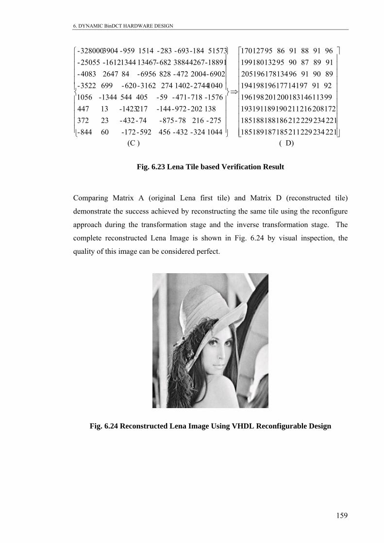
6. DYNAMIC BinDCT HARDWARE DESIGN
⎥⎥⎥⎥⎥⎥⎥⎥⎥⎥⎥⎤
⎢⎢⎢⎢⎢⎢⎢⎡
⇒
⎪⎪
⎪⎪⎪⎪⎪
⎬
⎫
172 208 216 211 190 189 191 193 99 113 146 183 200 201 198 196 92 91 97 141 177 196 198 194 89 90 91 96 134 178 196 205 91 89 87 90 95 132 180 199 96 91 88 91 86 95 127 170
- 216 78- 875- 74- 432- 23 138 202- 972- 144- 217 1423- 13
1576- 718- 471- 59- 405 544 1344- 1040 2744- 1402 274 3162- 620- 699 6902- 2004 472- 828 6956- 84 2647 18891- 4267 3884 682- 13467 1344 1612- 5 51573 184- 693- 283- 1514 959- 3904 28000
⎦⎢⎢⎢⎢
⎣⎪⎪⎪
⎭⎪⎪⎪⎪
⎪⎪⎪⎪⎪
⎨
⎧
221 234 229 211 185 187 189 185 221 234 229 212 186 188 188 185
1044 324- 432- 456 592- 172- 60 844- 275 372
447 1056 3522- 4083-
2505-3-
(C ) ( D)
Compa
demon
approa The
omplete reconstructed Lena Image is shown in Fig. 6.24 by visual inspection, the
⎪⎩
Fig. 6.23 Lena Tile based Verification Result
ring Matrix A (original Lena first tile) and Matrix D (reconstructed tile)
strate the success achieved by reconstructing the same tile using the reconfigure
ch during the transformation stage and the inverse transformation stage.
c
quality of this image can be considered perfect.
Fig. 6.24 Reconstructed Lena Image Using VHDL Reconfigurable Design
159

6. DYNAMIC BinDCT HARDWARE DESIGN
6.8.2 Tile Image
napshot simulation for the forward transformation of the Tile image is shown in Fig.
ce the Tile image contains constant tiles across each column, the index value to
e generated by the Entropy selection technique is always as expected is C9. The
eneric InvBinDCT snapshot shown in Fig. 6.26 is also emphasise constant use of
onfiguration 9 for the whole period of the simulation to reconstruct the image. The
erification process, explained earlier, conducted for last tile of this image is also shown
Fig. 6.27. The perfect reconstruction of the same tile is clearly observed when
age using the proposed novel reconfigurable transformation approach is shown in
ig. 6.28.
S
6.25. Sin
b
g
c
v
in
comparing Matrix (A) and (D) in Fig. 6.27. The perfect reconstructed of a complete Tile
im
F
Fig. 6.25 Timing Simulation For Tile Image During Forward Transformation
Operation
Fig. 6.26 Timing Simulation For Tile Image During Inverse Transformation Operation
160

6. DYNAMIC BinDCT HARDWARE DESIGN
(A) (B)
⎪
⎬
⎫
⎪
⎪
⎪
⎨
⎧
0 0 0 0 0 0 0 0 0 0 0 0 0 0 0 0 0 0 0 0 0 0
0 0 0 0 0 0 0 520192-⎥
⎦
⎤
⎢⎢⎢⎢⎢⎢⎢⎢
⎢
⎣
⎡
254 254 254 254 254 254 254 254 254 254 254 254 254 254 254 254 254 254 254 254 254 254 254 254 254 254 254 254 254 254 254 254 254 254 254 254 254 254 254 254
254 254 254 254 254 254 254 254
(D)
f Tile Image Verification Result
⇒
⎪⎪⎪⎪⎪
⎭
⎪⎪⎪⎪
⎪⎪⎪⎪
0 0 0 0 0 0 0 0 0 0 0 0 0 0 0 0 0 ⎥
⎢⎢
254 254 254 254 254 254 254 254 254 254 254 254 254 254 254 254
⎪ 0 0 0 0 0⎪⎪ 0 0 0 0 0 0 0 0
⎩ 0 0 0 0
⎥⎥⎥⎥⎥⎥⎥⎥⎥
( C)
Fig. 6.27 Last Tile o
Fig. 6.28 Reconstructed Tile Image Using VHDL Reconfigurable Design
⎪⎪⎪⎫
⎪⎪
⎧
⎥⎥
⎤
⎢⎢
⎡
0 0 0 0 0 0 0 0 0 0 0 0 0 0
0 0 0 0 0 0 0 0 0 0 0 0 0 0 0 0 0 0 0 520192-
254 254 254 254 254 254 254 254
254 254 254 254 254 254 254 254⎪⎥⎢ 0 0 0 0 254 254 254 254 254 254 254 254
⎪⎪⎪⎪
⎪⎪⎪⎪
⎥⎥⎥⎥
⎢⎢⎢⎢
0 0
0 0 0 0 0 0 0 0
254 254 254 254 254 254 254 254 254 254 254 254 254 254 254 254 254 254 254 254 254 254 254 254
⎪
⎪⎪⎬
⎪
⎪⎪⎨⇔
⎥⎥⎥⎥
⎢⎢⎢⎢
0 0 0 0 0 0 0 0 0 0 0 0 0 0 0 0
254 254 254 254 254 254 254 254 254 254 254 254 254 254 254 254
⎭⎩⎦⎣
161

6. DYNAMIC BinDCT HARDWARE DESIGN
6.8.3 FPGA Hardware Implementation
Implementation of the generic FBinDCT using 4vlx15sf363-12 FPGA device was
discussed in section 6.4. Also the implementation of the generic InvBinDCT processor
was also discussed in section 6.5 for the same device. The utilisation of the compound
Entropy selection technique and the generic FBinDCT
processor within the same 4vlx15sf363-12 FPGA device were not met due to limited
size in the FPGA chip.
apped
to a specif
design was far too big to fit the design into ber of the
ic reconfiguration FBinDCT was 20930 out of
.
.9 Summary this chapter the two methods of implementing the proposed work of reconfiguring
inDCT algorithm in run time for both forward and inverse transformation stage were
iscussed. A number of images were used to test both systems. Simulation results as
ill as the reconstructed images were also listed. A very good quality images were
btained when using the reconfigurable approach.
To im
representing all configurations of the design n files
of the configuration then will be stored to an external memory. Each configuration then
will be read from the memory and loaded to the FPGA according to the current entropy
index value. The bottleneck of this process then will be the time required to access the
design that consists from
Investigating synthesis report when converting the RTL design into netlist to be m
ic FPGA device had revealed that the area utilisation required to map this
a single FPGA chip. The total num
slices required to conduct the dynam
6144 available in a single FPGA chip. This is equal to 340% of the available FPGA
hardware resource.
However the actual hardware FPGA implementation still can be achieved by partioning
the design and hence distribute the partition into multi-FPGA system device that
compromises of four FPGA chips. When connecting in serial pipeline fashion, each
FPGA device will be responsible for computing part of the design and dispatch the
result for the next FPGA chip to continue processing the rest of the algorithm
6In
B
d
w
o
plement the static BinDCT algorithm a total of eighteen different copies
eed to be constructed. The bit stream
162

6. DYNAMIC BinDCT HARDWARE DESIGN
memory and read the intended configuration bit stream. The other timing constraint will
e the FPGA reconfiguration time.
Implem
configu
parame
reconfi
the loo
with t
environ well as reducing the
tim required to execute the algorithm.
The d
techniq
FPGA
The fu
system ters. Discussion of the future works,
recomm ndations, and conclusion will follow in the next chapter.
b
enting the generic BinDCT algorithm on other hand require only one
ration with a lookup table that contains the pre-computed configuration
ters for the nine FBinDCT and the nine InvBinDCT algorithms. This
gurable approach will use the index values dispatched to the module to address
kup table and hence load the correct configuration parameter to be associated
he current tile. Implementing generic BinDCT within FPGA integrated
ment results on more area utilization of the FPGA chip as
e
ynamic reconfigurable system consists from combined Entropy selection
ue and the generic FBinDCT algorithm cannot be implemented on a single
device. However the design can be implemented on a multi-FPGA system.
ll details of the proposed novel run time reconfigurable BinDCT algorithm
is explained in previous chap
e
163

7. RECOMMENDATIONS FOR FUTURE WORK AND CONCLUSIONS
Chapter 7
RECOMMENDATIONS FOR FUTURE WORK AND
CONCLUSIONS
_______________________________________________________
troduction
h conducting this research, a potential improvement to the proposed work has
entified; future work to be conducted to implement the founded novel system in
re is suggested. Constructing dynamic or hybrid system that will be able to
between the lossy and lossless image compression during the run time based on
rmation derived from the incoming tile is also proposed for further research to
. Finally the summary and conclusions of the thesis are outlined.
rdware Im
_____
7.1 In
Throug
been id
hardwa
switch
the info
explore
7.2 Ha plementation
In chapter 6 of the thesis two architecture implementations of the BinDCT algorithm
were suggested; dynamic partial configuration and context switching techniques. Both
methods can be used to implement the full working model in hardware system
environment as follows:
can be used with both systems in different ways. If
the system requires to implement the static forward BinDCT algorithm, the
1. Context switching technique
FPGA will needs to download a new BinDCT configuration when ever a new
index different from the current index has arrived. For the generic reconfigurable
BinDCT system, although no need to change the configurations of the FPGA
completely during the forward operation, but the context switching will be done
to perform InvBinDCT processor operation to reconstruct the image and hence
display the image.
164

7. RECOMMENDATIONS FOR FUTURE WORK AND CONCLUSIONS
2. The dynamic reconfigurable configuration of the FPGA technique can be used
with the generic reconfigurable BinDCT system implementation. If all the
BinDCT configuration parameters are loaded to the external memory, the FPGA
have to replace the parameters of the current active configuration running in the
FPGA with the coefficient parameter of the BinDCT configuration that belongs
to the new calculated index value.
3. Novel Entropy selection technique can use the context switching technique
through partitioning the produce design configuration. Each sub-block
configuration will be loaded to the external memory for execution. The output of
this stage will be saved back to the external memory. The next sub-block
configuration in the pipeline then has to be loaded to the FPGA. Reconfiguration
of the FPGA has to continue to the end of the process to produce the index.
.2.1 System Overview: Single FPGA System Development Board To Implement
Suggested Context Switching and Dynamic Configuration.
The ha mory
and computer. The FPGA communicates with an external memory. A computer
he FPGA and the memory and is used to load the nine BinDCT
emory as well as downloading the novel Entropy selection
chnique and control configurations of the FPGA. RTR process is conducted as
2- Video interface board: frame grabber.
7
rdware needed to set up an RTR system in general consists of an FPGA, me
interacts with both t
configurations into the m
te
follows: first temporal partition gets input data or pixels, carries out computations and
stores the intermediate result into the system memory. The FPGA is then reconfigured
for the next sector that computes the outcomes based on the stored data from the
preceding partition. This procedure continues until all the partitions are completed. The
initial study for the project requirement to be implemented in hardware, expecting the
system component to be as shown in Fig. 7.1 and its main parts as listed below:
1- Camera: such as digital video camera.
3- Projector or PC for viewing.
4- Development board that has FPGA and RAMs: ML310 board.
165

7. RECOMMENDATIONS FOR FUTURE WORK AND CONCLUSIONS
PC
Fig. 7.1 The Generic Sy
GA and camera.
arket as low-end frame-grabber. Examples
A video interface or capture board acts as an in
camcorder, VCR, or CCD camera, with the FP
used for two reasons: some camera’s outputs i
frames from the video source. Also it s
synchronisation between FP
m
AIMS Labs (standard for screen capture that w
Snappy from Play Inc (captures images at re
1125)[66], and the Dazzle Digital Video Cr
Digital Video Camera
Video Capture Board
M310 development board contain the FPGA, RAMstem Components.
This interface board
of such products i
zzle
terface between a v
GA and with the PC
s not digital, the boa
olves the problem
orks with all version
cord-breaking resol
eator from Da
can be found in the
nclude Grab-It from
Multimedia (Dazzle
ideo source such as a
. This board can be
rd should digitise the
of the frame rate
s of Windows) [65],
utions up to 1500 x
166

7. RECOMMENDATIONS FOR FUTURE WORK AND CONCLUSIONS
DVC150 ideal Hi-Speed USB video editing system) [67]. Or it can be design using the
FPGA combined with DRAM.
tises the analogue video
source come from a camcorder, VCR or CCD camera. (e.g. VPX 3226E).
er until it
System control logic: this consists of all the logic necessary to manage the pixels
er to the
t concern this project
DR DIMM.
• 4 PCI slots (3.3V and 5V).
• Standard JTAG connectivity.
.2.2 Power Processor-FPGA System Development Board To Implement The
This system advised in 7.2.1 has two power cores PC405 which can be used to optimize
nd the area of the design. Since within the current design the most of the area
ovel
the
n in Fig.
7.2. The FPGA then will act upon the resulted index value to load the matching static
inDCT configuration from the external memory in the context switching operation
ideo interface board consists from three key functional parts [68]: V
Video Pixel decoder (VPX): this functional block digi
Frame buffer: The converted digitised frame has to be stored in the buff
can be sent to the FPGA for further processing.
flow direction from the VPX block to the buffer, and from the buff
parallel port.
The main features of the ML310 embedded development board tha
are stated below [69]:
• FPGA (type XC2VP30-FF896).
• Two Power PC405 cores.
• 256 MB D
• FPGA serial port connection.
7
Suggested Coupled Dynamic BinDCT System.
the speed a
utilization constrained were caused by the Entropy selection technique. The n
Entropy selection technique calculation to produce the index can be shifted outside
FPGA and executed using one of the two PC405 processors available as show
B
167

7. RECOMMENDATIONS FOR FUTURE WORK AND CONCLUSIONS
mode, or reconfigure the current FPGA configuration of the generic BinDCT system
peration
or of Xilinx ML310 board can help to reduce the time taken to
alculate the index and therefore the area of the selection technique would be preserved.
PC405 to Calculate The Selection Technique And FPGA to Calculate The
he actual hardware FPGA implementation without the use of any processors can be
achieved by partioning the design and hence distribute the partition between multi-
mpromises four FPGA chips as demonstrated in Fig. 7.3.
hen connecting in serial pipeline fashion, each one of the FPGA devices will be
responsible for computing part of the design and dispatch the result for the next FPGA
Fig. 7.3 Multi-FPGA System to Calculate The Combined Entropy Selection
with new parameters of the matching BinDCT configuration in dynamic o
mode. Power Process
c
CT or CT
Fig. 7.2
BinDCT Algorithm.
7.2.3 Multi-FPGA System Development Board
T
FPGA system device that co
W
device to continue processing the rest of the algorithm.
Technique And The FBinDCT Processor
PC405
Power processor
Index En opy selection trFPGA
Generic FBinDStatic FBinD
GLCM
Normalisation
FPGA FPGA
Index calculation And FBinDCT
FPGA
Log Function FPGA
168

7. RECOMMENDATIONS FOR FUTURE WORK AND CONCLUSIONS
7.3 Software Implementation
1. Throughout this project the choice of a particular transform in a given
application depends on the entropy value calculated for the incoming tile. The
Homogeneity selection technique were also proposed and tested in C
he results
ogeneity selection technique in section 4.5, I strongly
suggest to develop a hardware module to implement this technique. This will
Log
2. More selection techniques should be investigated in terms of more efficient
sts to try
trast,
omentum, Maximum
Probability, Standard Deviation, Uniformity, Mean value and the Variance for
able to
3. Further enhancement could be done by combining more than one measure in at
es are
both used to identify the best BinDCT configuration that suits the incoming tile
the RMSE value and the compression ratio may improve.
ivided into
he investigation to cover
different sizes such as (4×4) and (16×16) in order to be able to judge the most
programming language but not implemented in hardware. In line with t
obtained from the Hom
optimise both area and speed over the Entropy selection technique since no
function will be needed before producing the index value.
hardware implementation and software performance. The author sugge
to create a new selection techniques using other measures such as Con
Correlation, Different Momentum, Inverse Different M
each incoming tile, all the above mentioned measured should also be
decide the tile index value.
same time, therefore if the Entropy and Homogeneity selection techniqu
4. The work done in this project always assumes that the image will be d
tiles of size 8×8 pixels. I suggest extending further t
suitable size with minimum root mean square error and best reconstructed image
quality.
169

7. RECOMMENDATIONS FOR FUTURE WORK AND CONCLUSIONS
rk
database of the system as explained in section 4.3. For further enhancement of
the design giving the decision of which configuration is to consider the best
not be
figurations
in row-wise and the second stage operation work in column wise, the RMSE
this first Entropy selection technique can be calculated before performing the
ge.
be
gorithm suits the tile processed by
the first BinDCT stage and form input to the second stage of the BinDCT
stigate the efficiency of using both Entropy and Homogeneity selection
techniques with different configuration of Loffer BinDCT proposed architecture.
Coding gain may improve since he proposes BinDCT implementation with less
e
ackground is constant and therefore does not contain important information. I suggest
The
techniques when operates on constant tiles produces the same image compression ratio.
The output of all BinDCT configuration always produce a DC value and 63 AC zeros
5. Although BinDCT algorithm is a two dimensional transform function, this wo
was only used the coefficients outputted by the second dimension of the
transform function to calculate the RMSE value and hence constructing the
solution for each tile after calculating the forward 2-D BinDCT only, may
completely right. The best selection for each tile could be two con
instead of only one. Because the first stage of the 2D-BinDCT operation works
value can be calculated twice for each tile, one for each BinDCT dimension
operation. Also the selection technique can be calculated twice. According to
first dimensional and then again before performing the second dimension sta
The configuration suits the original row image tile frequency content, could
different from the BinDCT configuration al
operation.
6. Inve
number of add and shift operations to perform the transform.
7.4 Proposing New System
Since not all part of the medical image that uses the lossless image technique have th
same important information to keep, for example some times most part of the image
b
developing a dynamic Lossy-Lossless compression system as shown in Fig. 7.4.
results obtained from chapter 3 shows that lossy and Lossless image compression
170

7. RECOMMENDATIONS FOR FUTURE WORK AND CONCLUSIONS
for each constant tile for both compression techniques. Therefore when loosy technique
,
and the amount of the information will be lost according to this scaling will not be
important if the tile in the original image is constant and located in the background.
herefore if the novel Entropy or Homogeneity selection techniques developed in this
thesis can be used to detect in advance if the incoming tile is constant as they do and
ssless compression technique, in which a
ast majority of confidential and medical sectors can benefit from the advantages gained
ssion
technique.
propose a novel pre-processing technique to be
sed with the image compression system has been achieved. Detail investigation for the
ng
Discrete Cosine Transform (BinDCT) algorithm performed on
e incoming tile. The calculated Entropy or Homogeneity values during run-time
re
the hardware implementation of the BinDCT
lgorithm have been proposed. For the static BinDCT a total of 18
is implemented the DC term of the transformed coefficient, tile will be scaled down
T
therefore inform the system to use lossy or lo
v
in storage or transmission time when using lossy over lossless image compre
Lossy image
Fig. 7.4 Proposed Dynamic Loosy-Lossless Image Compression System
7.5 Conclusions
The principal aim of this research to
u
novel tile based detecting methods such as Entropy and Homogeneity selection
techniques were produced. The novel techniques will work as a run-time pre-processi
stage before the Binary
th
operation will be used to inform the BinDCT system which configuration is mo
efficient to be used with the incoming tile and therefore reconfigure accordingly.
Two different functional description of
a
Selection technique
compression Incoming tile
Lossless image compression
171

7. RECOMMENDATIONS FOR FUTURE WORK AND CONCLUSIONS
FBinDCT/InvBinDCT configurations were created. For the generic BinDCT system
g from the Entropy selection technique and the generic
rward BinDCT processor behaves as a Dynamic Reconfigurable BinDCT system that
T with
pression ratio will be
btained if the proposed technique used with the Lossless over using a single BinDCT
configuration to transform the whole image. Lossy results were also satisfying since the
e
ilar RMSE value. A
erfect reconstruction for the processed image using the dynamic reconfigurable
loosy
and lossless techniques. For constant images both lossy and lossless techniques generate
ber of clock cycles required to calculate and hence produce new
ocessor
to finish transforming the incoming tile. The total clock cycles required for each tile to
pression will always produce
age for the Homogeneity and the entropy
eity
r not quantized constant images is zero.
Therefore for constant images the use of the quantized images (lossy compression) will
only one FBinDCT and one InvBinDCT configuration were created. The coupled
combined system consistin
fo
uses the output of the novel selection technique to reconfigure the generic BinDC
the new configuration parameter.
Dynamic reconfigurable BinDCT system performed well with both lossy and lossless
image compression techniques. Test results show that the best com
o
dynamic reconfigurable technique produce compression ratio nearly equivalent to th
best approximation of the DCT configuration with nearly sim
p
BinDCT system were obtained from both C and VHDL implementations for both
the same compression ratio.
The total num
configuration index value using the Entropy selection technique is 140 for each tile in
the image. The system needs to wait further 153 clock cycles for the BinDCT pr
completely processed using this technique is 293 clock cycles.
Operating on non-quantized images for lossless image com
successful full reconstruction of the im
selection techniques.The reconstructed images through using Entropy and Homogen
selection techniques always produce lower RMSE than using the configuration BinDCT
9 for the quantized images.
The reconstruction RMSE for the quantized o
be more beneficial in terms of storage and transmission time.
172

Reference
REFERENCE
____________________________________________________________ [1]. William B.Pennebaker, Joan L. Mitchell , JPEG Still Image Data
ao, K.R “ Discrete Cosine Transform ”. IEEE
Transaction on Computer, January 1974, pp.90-93.
Using
Dynamic FPGAs”. PhD thesis, Liverpool John Moores University 2002.
n of the BinDCT”,Liverpool John Moorse University,2003.
4-
]. Duhamel, P.; H´Mida, H.: New 2n DCT Algorithms, suitable for VLSI
Implementation Proceedings IEEE International conference on Acoustics,
ations of the DCT with the
lifting scheme” Signal Processing, IEEE Transactions on Acoustics, Speech,
–
3044.
Compression Standard, 1993 by Van Nostrand Reinhold.
[2]. Ahmed, N.; Natarajan, T; R
[3]. C.W. Murphy Run-time “Re-configurable DSP Processing System
[4]. C.W.Murphy, D.M.Harvey “Novel Reconfigurable Hardware
Implementatio
[5]. C.W.Murphy, D.M.Harvey “ Reconfigurable Hardware Implementation of
BinDCT”, IEE Electronics Letters, Vol. 38, No. 18, August 2002, pp.
1012-1013.
[6]. W. Chen, C.H.Smith, and S.C.Fralick,”A fast computational algorithm for
The Discrete Cosine transform ”IEEE, Trans.Commun.COMM-25, pp.100
1009, Sep.1977.
[7
Speech and, Signal Processing, ICASSP-87, Dallas, April 1987,pp. 1805-
1808.
[8]. Jie Liang; Tran, T.D.“Fast multiplierless approxim
and Signal Processing, Volume 49, Issue 12, Dec. 2001 Page(s):3032
173

Reference
[9]. B. G. Lee, “A new algorithm to compute the discrete cosine transform,”
IEE Proc., vol. 128, pt. F, no. 6, pp. 359-360, Nov.1981.
thms for the
ar .Conf.
Circuit, Syst., Comput., PacificGrove, CA, Nov. 1985.
[12]. N. Suehiro and M. Hatori, “Fast algorithms for the DFT and other sinusoidal transforms,” IEEE Trans. Acoust., Speech, Signal Processing,
. Pearson, “Fast cosine transform implementation for television signals,” IEE Proc-F, vol. 129, no. 1, pp. 59- 68, Feb. 1982.
[14]. M. Vetterli,“Fast 2-D discrete cosine transform,” in Proc. ICASSP, Mar.
1985, pp.1538– 1541.
erg, A. Moschytz, G.S.” Practical, Fast 1D- DCT
Algorithms with 11 Multiplications.” IEEE Proc. Int´l Conf. on Acoustics,
Speech, and Signal Processing 1989, ICASSP-89, pp. 988-991.
[16]. Z. Wang, “Fast algorithm for the discrete W transform and for the discrete
Fourier Transform,” IEEE Trans. Acoust., Speech, Signal Processing, vol.
ASSP-32, pp.803–816, Aug. 1984.
[17]. R. M. Haralick, “A storage efficient way to implement the discrete cosine
transform,” IEEE Trans. Comput., vol. C-25, pp. 764-765, July 1976.
[18 ]. B. D. Tseng and W. C. Miller, “On computing the discrete cosine
transform,”.IEEE Trans. Comput., vol. C-27, pp. 966-968, Oct 1978.
IEEE Trans. Acoust., speech, Signal Processing, vol. ASSP-32, pp.1243–
1245, Dec.1984.
[10]. R. J. Clark, “Relation between the Karhunen-Lobe and cosine transform,”
[11]. N. Chelemal-D and K. R. Rao, “Fast computational algori
Discrete cosine transform,” presented at the 9th Annu. Asilom
vol. ASSP-34, pp. 642-644, Jun.: 1986. [13]. M. Ghanbari and D. E
[15]. Loeffler, C.; Ligtenb
174

Reference
[19]. M. J. Narashimha and A. M. Peterson, “On the computation of the discrete
cosine transform,” IEEE Trans COM-26, pp. 934-936, June
[20]. M. Vetterli and H. Nussbaumer, “Simple FFT and DCT algorithms with
reduced number of operations,” Signal Processing, vol. 6, no. 4, pp. 267-
278, AUg. 1984.
[21]. D. Hein and N. Ahmed, “On a real-time Walsh-Hadamard cosine transform
Image processor,” IEEE Trans. Electromagn. Compat., 4, pp. 267-278,
Aug. 1984. VOI. EMC-20, pp. 453-457, Aug. 1978.
[22]. B. G. Kashef and A. Habibi, “Direct computation of higher-order DCT
coefficients from lower-order DCT coefficients,” presented at the SPIE 28th
Annu. Int. Tech. Symp., San Diego, CA, Aug. 19-24, 1984
ive algorithm for computing the discrete cosine
transform,” IEEE Trans. Acoust., Speech, Signal Processing, vol.ASSP-35,
pp. 1455–1461, Oct. 1987.
[24]. Stanley A. white, “Applications of Distributed Arithmetic to Digital signal
Processing : A Tutorial Review ”IEEE ASSP Magazine, vol. 6. no. 3, July 1989.
[25]. Sungwook Yu “DCT implementation with Distributed Arithmetic”. IEEE
Transactions on Computers Volume 50, Issue 9 September 2001 Pages:
985 – 991, year of Publication: 2001 ISSN: 0018-9340.
[26]. Yuk-Hee Chan “on the realization of Discrete cosine transform “September 1992,
IEEE Transaction on circuit and systems. Volume 39 number 9, ITCAEX ISSN
1057-7122.
[27]. N. Demassieux, G. Concordel, J. P. Durandeau, and F. Jutand,” optimized VLSI
architecture for multiformat discrete cosine transform.” In Proc.ICASSP’87,pp.
547-550, Apr. 1987.”
. Commun., vol.
1978.
[23]. H. S. Hou, “A fast recurs
175
Reference
[28]. A. Artieri, S. Kritter, F.Jutand, and N. Demassieux, “A one chip VLSI for real
time two-dimensional discrete cosine transform” in Proc.ISCAS’88, pp. 701_704,
June 1988.
[29]. In-Cheol Park, Hyeong-Ju Kang “Digital filter synthesis based on minimal signed
digit representation “ Annual ACM IEEE Design Automation Conference
Proceedings of the 38th conference on Design automation Las Vegas,
Nevada, United States Pages: 468 – 473 , Publication: 2001 ISBN:1-58113-297-2.
[30]. Y. C. Lim, J. B. Evans, and B. Liu, “Decomposition of binary integers into signed
power-of-two terms,” IEEE Trans. Circuits Syst., vol. 38, no. 6, pp. 667-672,1991.
[31]. R. Hashemian, “A new method for conversion of a 2’s complement to canonic
signed Digit number system and its representation,” in Proc. Asilomar Conf.
Signals, Syst., Computers, 1997, pp. 904-907.
[32]. Trevor W. Fox-2002 “Rapid Prototyping of Field Programmable Gate Array-
Based Discrete Cosine Transform Approximations” EURASIP JASP 2003, 543-
554.
[33]. Jongsun Park”A low power reconfigurable DCT Architecture to trade off image
quality for computational complexity” IEEE International Conference on
Acoustics, Speech and Signal Processing (ICASSP2004.1327036), Montreal,
Canada, May, 2004Pages: 17-20 vol.5.
[34]. Richard I. Hartley-1996 “Subexpression Sharing in filter using Canonic Signed
Digit Multipliers” IEEE Trans. Circuits Syst. II, vol. 43, no. 10, pp. 677-688, 1996.
[35]. Anthony Edward Nelson “Implementation of image processing algorithms on
FPGA hardware” thesis of Master of Science in Electrical Engineering, May 2000
Graduate School of Vanderbilt University.
[36]. http://www.takimaging.com/products/takb4.php 17/September/2005.
176

Reference
[37]. http://www.eetimes.com/story/OEG20000814S0033. “adaptable computing right
For MPEG-4”. 17/September/2005.
[38]. Latha Pillai.” video compression using DCT”, XILINX Application Note : Virtex-
11 series.XAPP610,v1.2, April 24,2002.
[39]. Daniel Bayeh” Implementation of a fast 2D DCT for FPGA”, Master thesis,
University of Hertfordshire, Department of electrical, com unication and
electronics engineering, Augu
[40]. D.W. Trainor, J.P. Heron and R.F. Woods “Implementation of the 2D DCT using
A Xilinx XC6264 FPGA” integrated silicon systems ltd .
[41]. Gustavo Andre Hoffman; Eric Ericson Fabris; Diogo Zandonai; Sergio Bampi
UFRGS Federal Univ- Microelectronics Group “the BinDCT processor”
[42]. Sambandan Sachidanadan “Design, implementation and testing of 8x8 DCT chip”.
Master thesis, University of Maryland, college park, MD. 20742-1989.
[43]. Choomchuay S. and Timakul S., "A Bit-Serial Architecture for a Multiplierless
DCT," Journal of Information and Communication Technology, University Utara
Malaysia, Vol. 2(1), Jun. 2003.
[44] Y.H.Chan and W.C.Siu, "On the realizati screte cosine transform using the
distributed arithmetic", IEEE trans. on Circuits and Systems, Vol.39, No.9, Sep
1992, pp.705-712.
[45]. Philip P.Dang,Truong Q.Nguyen,Trac D.Tran,John Hopkin“ High-performance
Low-power BinDCT processor for Wireless Video Application” Real-Time
Imaging VIII . California; Proceedings of SPIE Vol. #5297, May 18, 2004; p. 254-
263; ISBN / ISSN: 0- 8194-5200-9.
m
st 04.
on of di
177
Reference
[46]. S. Chuntree and S. Choomchuay, "A Bit-Parallel Pipelined Multiplierless DCT,"
EECON-26, King Mongkut's Institute of Technology, North Bangkok, November
2003, pp. 1173-1178.
[47]. Claus Schneider , Martin Kayss , Thomas Hollstein ‡ gen Deicke ‡ “From
algorithms to hardware architectures: a comparison of regular and irregular
structured IDCT algorithms .”Proceedings of the conference on Design,
automation and test in Europe Le Palais des Congrés de Paris, France Pages:
186 - 190 Year of Publication: 1998 ISBN:0-8186-8359-7.
[48]. Shih-Chang Hsia et al-1995,“VLSIImplementation of Parallel Coefficient by
Coefficient Two Dimensional IDCT Processor” IEEE Tansaction on circuit and
systems for Video Technology,Vol. 5,No. 5, October 1995.
[49]. A.J.Carter,“Architecture for Dynamic Reconfigurable Real-time Lossless
Compression”. Real-Time Imaging VIII California; Proceedings of SPIE Vol.
5297, May 18, 2004; ISBN / ISSN: 0- 8194-5200-9.
[50]. Olof Larsson, Oscar Johnsson “implementation of Motion-JPEG Using an ASIC
Prototype Board”. Lund Institute Technology. Master Thesis 2001-12-17.
[51]. John Spillane, Henry Owen: Temporal Partitioning for Partially Reconfigurable
Field Programmable Gate Arrays, Georgia Institute of Technology, Department of
Electrical and Computer Engineering, Atlanta.
[52]. Meenakshi Kaul et al. “an anutomated temporal partitioning and loop fission
approach for FPGA reconfigurable synthesis of DSP applications” Annual ACM
IEEE Design Automation Conference Proceedings of the 36th ACM/IEEE
conference on Design New Orleans, Louisiana, United States Pages: 616-622,
Publication: 1999 ISBN:1-58133-109-7
[53]. Virtex-2 Pronand Virtex-2 ProX FPGA User Guide”P3362- 365.UG012,v4.0,23
March 2005.
178

Reference
[54]. Fuji, T. et al.(1999). A dynamically reconfigurable logic engine with a multi-
context multi-mode unified cell architecture. In Proc. Of Int. Solid-State Circuits
Conf, Pages 360-361.
[55]. Scalera, S. and Vazques, J.(1998). The design and implementation of context
switching FPGA. In IEEE symposium on FPGAs for Custom Computing
Machines, pages 78-85. [56]. Shannon, C. E.,”A Mathematical Theory of communication”. Bell system
Technical Journal, Vol.27 pp.379-423, pp. 623-656, July 1948.
[57]. R.M.Haralick, K.Shanmugam age
Classification”, , IEEE Transactions on Systems, Man and Cybernetics, 1973,
p.610-621.
[58]. M.A. Tahir, A. Bouridane F. Kurugollu, and A. Amira ”An FPGA based
Coprocessor for Calculating Grey Level Co-Occurrence Matrix” Proceedings of
the IEEE Midwest Symposium on Circuits and Systems, Cairo, Egypt, December
27-30,2003.
[59]. M.A. Tahir, A. Bouridane and F. Kurugollu, A. Amira “Accelerating the
Computing of GLCM and Haralick Texture Features on Reconfigurable
Hardware” Proceeding of the IEEE International Conference of Image Processing
(ICIP), October 24-27,2004.
[60]. M.A. Tahir, A. Bouridane F. Kurugollu, and A. Amira “An FPGA Based
Coprocessor for GLCM and Haralick Texture Feature and their Application in
Prostate Cancer Classification “.Analog Integrated Circuit and Signal
Processing. SJNW123-10-205, February 2005.
[61]. Model Sim LE/PE Tutorial Software Version 6.2g, February 2007.
[62]. www.xilinx.com
, I.Dinstein “Textural Features for Im
.
179

Reference
[63]. Ray Andraka “A survey of CORDIC algorithm for FPGA based computers”.
International Symposium on Field Programmable Gate Arrays. Proceedings of the
1998 ACM/SIGDA sixth international symposium on Field programmable gate
arrays Pages: 191 - 200 Year of Publication: 1998 ISBN:0-89791-978-5
[64]. Volder, J.”The CORDIC Trigonometric Computing Technique”. IRE Trans.
Electronic Computing, Vol. EC-8, Sept. 1959, pp330-334
[65]. http://www.sebd.com/grabit_pro.html 17/September/2005.
[66].http://www.omegamultimedia. /snappy4.htmcom/products/play 17/September/2005.
[67]. http://www.pinnaclesys.com/publicsite/uk/Products/DazzleHome/
17/September/2005.
[68]. Xilinx application note XAPP172 March 31, 1999 (Version 1.0)” The Design of a
Video Capture Board Using the Spartan Series”.
[69].http://www.xilinx.com/products/boards/ml310/current/index.html
17/September/2005.
180

Appendix
181
APPENDIX
____________________________________________________________ The image files used to establish the data base to calculate the threshold points as well as to test proposed novel Entropy and Homogeneity selection techniques are shown below:
Mahmoudtiles Image
Alaqsa Image

Appendix
182
Canadaneqaraqwa Image
Coins Image
Gray Image

Appendix
183
Zebra Image
Building Image

Appendix
184
Vegi (Formatbitmapcolour)
House Image
Light Image

Appendix
185
Madina Image
Mahmoud Image
Mahmoud in the sea Image
Appendix
186
Makka Image
Rose Image
Texture Image

Appendix
187
Texture0 Image
Texture 1 Image
Texture 2 Image

Appendix
188
Texture3 Image
Texture4 Image
Tile Image


![Abstract - Index terms - IJSER...model can be done using ASIC’s or FPGA’s. The latter is developed by the authors[4].The use of FPGA’s extends more flexibility to the design](https://static.fdocuments.in/doc/165x107/5e4dee5581ffa45a463ef04f/abstract-index-terms-ijser-model-can-be-done-using-asicas-or-fpgaas.jpg)