
Image Compression: The Mathematics of JPEG 2000library.msri.org/books/Book46/files/08li.pdf ·...
37
Modern Signal Processing MSRI Publications Volume 46, 2003 Image Compression: The Mathematics of JPEG 2000 JIN LI Abstract. We briefly review the mathematics in the coding engine of JPEG 2000, a state-of-the-art image compression system. We focus in depth on the transform, entropy coding and bitstream assembler modules. Our goal is to present a general overview of the mathematics underlying a state of the art scalable image compression technology. 1. Introduction Data compression is a process that creates a compact data representation from a raw data source, usually with an end goal of facilitating storage or trans- mission. Broadly speaking, compression takes two forms, either lossless or lossy, depending on whether or not it is possible to reconstruct exactly the original datastream from its compressed version. For example, a data stream that con- sists of long runs of 0s and 1s (such as that generated by a black and white fax) would possibly benefit from simple run-length encoding, a lossless technique replacing the original datastream by a sequence of counts of the lengths of the alternating substrings of 0s and 1s. Lossless compression is necessary for situ- ations in which changing a single bit can have catastrophic effects, such as in machine code of a computer program. While it might seem as though we should always demand lossless compres- sion, there are in fact many venues where exact reproduction is unnecessary. In particular, media compression, which we define to be the compression of im- age, audio, or video files, presents an excellent opportunity for lossy techniques. For example, not one among us would be able to distinguish between two images which differ in only one of the 2 29 bits in a typical 1024 × 1024 color image. Thus distortion is tolerable in media compression, and it is the content, rather than Keywords: Image compression, JPEG 2000, transform, wavelet, entropy coder, subbitplane entropy coder, bitstream assembler. 185
-
Upload
nguyenthien -
Category
Documents
-
view
217 -
download
0
Transcript of Image Compression: The Mathematics of JPEG 2000library.msri.org/books/Book46/files/08li.pdf ·...

Modern Signal ProcessingMSRI PublicationsVolume 46, 2003
Image Compression:The Mathematics of JPEG 2000
JIN LI
Abstract. We briefly review the mathematics in the coding engine ofJPEG 2000, a state-of-the-art image compression system. We focus indepth on the transform, entropy coding and bitstream assembler modules.Our goal is to present a general overview of the mathematics underlying astate of the art scalable image compression technology.
1. Introduction
Data compression is a process that creates a compact data representationfrom a raw data source, usually with an end goal of facilitating storage or trans-mission. Broadly speaking, compression takes two forms, either lossless or lossy,depending on whether or not it is possible to reconstruct exactly the originaldatastream from its compressed version. For example, a data stream that con-sists of long runs of 0s and 1s (such as that generated by a black and whitefax) would possibly benefit from simple run-length encoding, a lossless techniquereplacing the original datastream by a sequence of counts of the lengths of thealternating substrings of 0s and 1s. Lossless compression is necessary for situ-ations in which changing a single bit can have catastrophic effects, such as inmachine code of a computer program.
While it might seem as though we should always demand lossless compres-sion, there are in fact many venues where exact reproduction is unnecessary. Inparticular, media compression, which we define to be the compression of im-age, audio, or video files, presents an excellent opportunity for lossy techniques.For example, not one among us would be able to distinguish between two imageswhich differ in only one of the 229 bits in a typical 1024×1024 color image. Thusdistortion is tolerable in media compression, and it is the content, rather than
Keywords: Image compression, JPEG 2000, transform, wavelet, entropy coder, subbitplaneentropy coder, bitstream assembler.
185
186 JIN LI
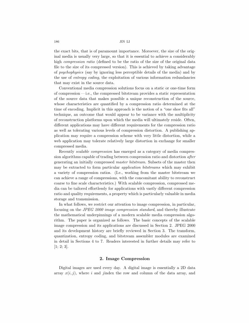
the exact bits, that is of paramount importance. Moroever, the size of the orig-inal media is usually very large, so that it is essential to achieve a considerablyhigh compression ratio (defined to be the ratio of the size of the original datafile to the size of its compressed version). This is achieved by taking advantageof psychophysics (say by ignoring less perceptible details of the media) and bythe use of entropy coding, the exploitation of various information redundanciesthat may exist in the source data.
Conventional media compression solutions focus on a static or one-time formof compression — i.e., the compressed bitstream provides a static representationof the source data that makes possible a unique reconstruction of the source,whose characteristics are quantified by a compression ratio determined at thetime of encoding. Implicit in this approach is the notion of a “one shoe fits all”technique, an outcome that would appear to be variance with the multiplicityof reconstruction platforms upon which the media will ultimately reside. Often,different applications may have different requirements for the compression ratioas well as tolerating various levels of compression distortion. A publishing ap-plication may require a compression scheme with very little distortion, while aweb application may tolerate relatively large distortion in exchange for smallercompressed media.
Recently scalable compression has emerged as a category of media compres-sion algorithms capable of trading between compression ratio and distortion aftergenerating an initially compressed master bitstream. Subsets of the master thenmay be extracted to form particular application bitstreams which may exhibita variety of compression ratios. (I.e., working from the master bitstream wecan achieve a range of compressions, with the concomitant ability to reconstructcoarse to fine scale characteristics.) With scalable compression, compressed me-dia can be tailored effortlessly for applications with vastly different compressionratio and quality requirements, a property which is particularly valuable in mediastorage and transmission.
In what follows, we restrict our attention to image compression, in particular,focusing on the JPEG 2000 image compression standard, and thereby illustratethe mathematical underpinnings of a modern scalable media compression algo-rithm. The paper is organized as follows. The basic concepts of the scalableimage compression and its applications are discussed in Section 2. JPEG 2000and its development history are briefly reviewed in Section 3. The transform,quantization, entropy coding, and bitstream assembler modules are examinedin detail in Sections 4 to 7. Readers interested in further details may refer to[1; 2; 3].
2. Image Compression
Digital images are used every day. A digital image is essentially a 2D dataarray x(i, j), where i and jindex the row and column of the data array, and

IMAGE COMPRESSION: THE MATHEMATICS OF JPEG 2000 187
x(i, j)is referred to as a pixel. Gray-scale images assign to each pixel a singlescalar intensity value G, whereas color images traditionally assign to each pixela color vector (R,G, B), which represent the intensity of the red, green, andblue components, respectively. Because it is the content of the digital imagethat matters, the underlying 2D data array may undergo big changes while stillconveying the content to the user with little or no perceptible distortion. Anexample is shown in Figure 1. On the left the classic image processing test caseLena is shown as a 512 × 512 grey-scale image. To the right of the originalare several applications, each showing different sorts of compression. The firstapplication illustrates the use of subsampling in order to fit a smaller image (inthis case 256×256). The second application uses JPEG (the predecessor to JPEG2000) to compress the image to a bitstream, and then decode the bitstream backto an image of size 512×512. Although in each case the underlying 2D data arrayis changed tremendously, the primary content of the image remains intelligible.
Image (512x512)
Subsample (256x256)Manipulation
Compress (JPEG)
167 123
84 200
2D array of data
ENC
DEC
Figure 1. Souce digital image and compressions.
Each of the applications above results in a reduction in the amount of sourceimage data. In this paper, we focus our attention on JPEG 2000, which is anext generation image compression standard. JPEG 2000 distinguishes itselffrom older generations of compression standards not only by virtue of its highercompression ratios, but also by its many new functionalities. The most noticeableamong them is its scalability. From a compressed JPEG 2000 bitstream, it ispossible to extract a subset of the bitstream that decodes to an image of variablequality and resolution (inversely correlated with its accompanying compressionratio), and/or variable spatial locality.
Scalable image compression has important applications in image storage anddelivery. Consider the application of digital photography. Presently, digital

188 JIN LI
cameras all use non-scalable image compression technologies, mainly JPEG. Acamera with a fixed amount of the memory can accommodate a small numberof high quality, high-resolution images, or a large number of low quality, low-resolution images. Unfortunately, the image quality and resolution must bedetermined before shooting the photos. This leads to the often painful trade-offbetween removing old photos to make space for new exciting shots, and shootingnew photos of poorer quality and resolution. Scalable image compression makespossible the adjustment of image quality and resolution after the photo is shot,so that instead, the original digital photos always can be shot at the highestpossible quality and resolution, and when the camera memory is filled to capacity,the compressed bitstream of existing shots may be truncated to smaller sizeto leave room for the upcoming shots. This need not be accomplished in auniform fashion, with some photos kept with reduced resolution and quality,while others retain high resolution and quality. By dynamically trading betweenthe number of images and the image quality, the use of precious camera memoryis apportioned wisely.
Web browsing provides another important application of scalable image com-pression. As the resolution of digital cameras and digital scanners continues toincrease, high-resolution digital imagery becomes a reality. While it is a plea-sure to view a high-resolution image, for much of our web viewing we’d trade theresolution for speed of delivery. In the absence of scalable image compressiontechnology it is common practice to generate multiple copies of the compressedbitstream, varying the spatial region, resolution and compression ratio, and putall copies on a web server in order to accommodate a variety of network situa-tions. The multiple copies of a fixed media source file can cause data managementheadaches and waste valuable server space. Scalable compression techniques al-low a single scalable master bitstream of the compressed image on the serverto serve all purposes. During image browsing, the user may specify a regionof interest (ROI) with a certain spatial and resolution constraint. The browserthen only downloads a subset of the compressed media bitstream covering thecurrent ROI, and the download can be performed in a progressive fashion so thata coarse view of the ROI can be rendered very quickly and then gradually refinedas more and more bits arrive. Therefore, with scalable image compression, it ispossible to browse large images quickly and on demand (see e.g., the Vmediaproject [25]).
3. JPEG 2000
3.1. History. JPEG 2000 is the successor to JPEG. The acronym JPEG standsfor Joint Photographic Experts Group. This is a group of image processing ex-perts, nominated by national standard bodies and major companies to work toproduce standards for continuous tone image coding. The official title of thecommittee is “ISO/IEC JTC1/SC29 Working Group 1”, which often appears in

IMAGE COMPRESSION: THE MATHEMATICS OF JPEG 2000 189
the reference document. The JPEG members select a DCT based image com-pression algorithm in 1988, and while the original JPEG was quite successful,it became clear in the early 1990s that new wavelet-based image compressionschemes such as CREW (compression with reversible embedded wavelets) [5]and EZW (embedded zerotree wavelets) [6] were surpassing JPEG in both per-formance and available features, such as scalability. It was time to begin torethink the industry standard in order to incorporate these new mathematicaladvances.
Based on industrial demand, the JPEG 2000 research and development effortwas initiated in 1996. A call for technical contributions was issued in March1997 [17]. The first evaluation was performed in November 1997 in Sydney,Australia, where twenty-four algorithms were submitted and evaluated. Follow-ing the evaluation, it was decided to create a JPEG 2000 “verification model”(VM) which was a reference implementation (in document and in software) ofthe working standard. The first VM (VM0) is based on the wavelet/trellis codedquantization (WTCQ) algorithm submitted by SAIC and the University of Ari-zona (SAIC/UA) [18]. At the November 1998 meeting, the algorithm EBCOT(embedded block coding with optimized truncation) was adopted into VM3, andthe entire VM software was re-implemented in an object-oriented manner. Thedocument describing the basic JPEG 2000 decoder (part I) reached committeedraft (CD) status in December 1999. JPEG 2000 finally became an internationalstandard (IS) in December 2000.
3.2. JPEG. In order to understand JPEG 2000, it is instructive to revisit theoriginal JPEG. As illustrated by Figure 2, JPEG is composed of a sequence offour main modules.
QUANRUN-LEVEL
CODINGFINAL
BITSTR
DCTCOMP &
PART
JPEG
Figure 2. Operation flow of JPEG.
The first module (COMP & PART) performs component and tile separation,whose function is to cut the image into manageable chunks for processing. Tileseparation is simply the separation of the image into spatially non-overlappingtiles of equal size. Component separation makes possible the decorrelation ofcolor components. For example, a color image, in which each pixel is nor-mally represented with three numbers indicating the levels of red, green andblue (RGB) may be transformed to LCrCb (luminance, chrominance red andchrominance blue) space.
190 JIN LI
After separation, each tile of each component is then processed separatelyaccording to a discrete cosine transform (DCT). This is closely related to theFourier transform (see [30], for example). The coefficients are then quantized.Quantization takes the DCT coefficients (typically some sort of floating pointnumber) and turns them into an integer. For example, simple rounding is aform of quantization. In the case of JPEG, we apply rounding plus a maskwhich applies a system of weights reflecting various psychoacoustic observationsregarding human processing of images [31]. Finally, the coefficients are subjectedto a form of run-level encoding, where the basic symbol is a run-length of zerosfollowed by a non-zero level, the combined symbol is then Huffman encoded.
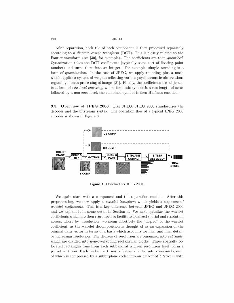
3.3. Overview of JPEG 2000. Like JPEG, JPEG 2000 standardizes thedecoder and the bitstream syntax. The operation flow of a typical JPEG 2000encoder is shown in Figure 3.
WAVELETQUAN &
PARTBITPLANE
CODING
BITSTR
ASSEMBLY
FINAL
BITSTR
COMP &
TILE
COLOR
IMAGE
Y COMP
CR COMP
CB COMP
Figure 3. Flowchart for JPEG 2000.
We again start with a component and tile separation module. After thispreprocessing, we now apply a wavelet transform which yields a sequence ofwavelet coefficients. This is a key difference between JPEG and JPEG 2000and we explain it in some detail in Section 4. We next quantize the waveletcoefficients which are then regrouped to facilitate localized spatial and resolutionaccess, where by “resolution” we mean effectively the “degree” of the waveletcoefficient, as the wavelet decomposition is thought of as an expansion of theoriginal data vector in terms of a basis which accounts for finer and finer detail,or increasing resolution. The degrees of resolution are organized into subbands,which are divided into non-overlapping rectangular blocks. Three spatially co-located rectangles (one from each subband at a given resolution level) form apacket partition. Each packet partition is further divided into code-blocks, eachof which is compressed by a subbitplane coder into an embedded bitstream with

IMAGE COMPRESSION: THE MATHEMATICS OF JPEG 2000 191
a rate-distortion curve that records the distortion and rate at the end of eachsubbitplane. The embedded bitstream of the code-blocks are assembled intopackets, each of which represents an increment in quality corresponding to onelevel of resolution at one spatial location. Collecting packets from all packetpartitions of all resolution level of all tiles and all components, we form a layerthat gives one increment in quality of the entire image at full resolution. Thefinal JPEG 2000 bitstream may consist of multiple layers.
We summarize the main differences:
(1) Transform module: wavelet versus DCT. JPEG uses 8 × 8 discrete cosinetransform (DCT), while JPEG 2000 uses a wavelet transform with liftingimplementation (see Section 4.1). The wavelet transform provides not onlybetter energy compaction (thus higher coding gain), but also the resolutionscalability. Because the wavelet coefficients can be separated into differentresolutions, it is feasible to extract a lower resolution image by using only thenecessary wavelet coefficients.
(2) Block partition: spatial domain versus wavelet domain. JPEG partitionsthe image into 16 × 16 macroblocks in the space domain, and then appliesthe transform, quantization and entropy coding operation on each block sep-arately. Since blocks are independently encoded, annoying blocking artifactsbecomes noticeable whenever the coding rate is low. On the contrary, JPEG2000 performs the partition operation in the wavelet domain. Coupled withthe wavelet transform, there is no blocking artifact in JPEG 2000.
(3) Entropy coding module: run-level coefficient coding versus bitplane coding.
JPEG encodes the DCT transform coefficients one by one. The resultant blockbitstream can not be truncated. JPEG 2000 encodes the wavelet coefficientsbitplane by bitplane (i.e., sending all zeroth order bits, then first order, etc.Details are in Section 4.3). The generated bitstream can be truncated at anypoint with graceful quality degradation. It is the bitplane entropy coder inJPEG 2000 that enables the bitstream scalability.
(4) Rate control: quantization module versus bitstream assembly module. InJPEG, the compression ratio and the amount of distortion is determined bythe quantization module. In JPEG 2000, the quantization module simplyconverts the float coefficient of the wavelet transform module into an integercoefficient for further entropy coding. The compression ratio and distortionis determined by the bitstream assembly module. Thus, JPEG 2000 canmanipulate the compressed bitstream, e.g., convert a compressed bitstreamto a bitstream of higher compression ratio, form a new bitstream of lowerresolution, form a new bitstream of a different spatial area, by operating onlyon the compressed bitstream and without going through the entropy codingand transform module. As a result, JPEG 2000 compressed bitstream can bereshaped (transcoded) very efficiently.

192 JIN LI
4. The Wavelet Transform
4.1. Introduction. Most existing high performance image coders in applica-tions are transform based coders. In the transform coder, the image pixels areconverted from the spatial domain to the transform domain through a linearorthogonal or bi-orthogonal transform. A good choice of transform accomplishesa decorrelation of the pixels, while simultaneously providing a representation inwhich most of the energy is usually restricted to a few (realtively large) coeffi-cients. This is the key to achieving an efficient coding (i.e., high compressionratio). Indeed, since most of the energy rests in a few large transform coeffi-cients, we may adopt entropy coding schemes, e.g., run-level coding or bitplanecoding schemes, that easily locate those coefficients and encodes them. Becausethe transform coefficients are highly decorrelated, the subsequent quantizer andentropy coder can ignore the correlation among the transform coefficients, andmodel them as independent random variables.
The optimal transform (in terms of decorrelation) of an image block can bederived through the Karhunen–Loeve (K-L) decomposition. Here we model thepixels as a set of statistically dependent random variables, and the K-L basis isthat which achieves a diagonalization of the (empirically determined) covariancematrix. This is equivalent to computing the SVD (singular value decomposition)of the covariance matrix (see [28] for a thorough description). However, the K-Ltransform lacks an efficient algorithm, and the transform basis is content depen-dent (in distinction, the Fourier transform, which uses the sampled exponentials,is not data dependent).
Popular transforms adopted in image coding include block-based transforms,such as the DCT, and wavelet transforms. The DCT (used in JPEG) has manywell-known efficient implementations [26], and achieves good energy compactionas well as coefficient decorrelation. However, the DCT is calculated indepen-dently in spatially disjoint pixel blocks. Therefore, coding errors (i.e., lossycompression) can cause discontinuities between blocks, which in turn lead toannoying blocking artifacts. In contrary, the wavelet transform operates on theentire image (or a tile of a component in the case of large color image), whichboth gives better energy compaction than the DCT, and no post-coding blockingartifact. Moreover, the wavelet transform decomposes the image into an L-leveldyadic wavelet pyramid. The output of an example 5-level dyadic wavelet pyra-mid is shown in Figure 4.
There is an obvious recursive structure generated by the following algorithm:lowpass and highpass filters (explained below, but for the moment, assume thatthese are convolution operators) are applied independently to both the rows andcolumns of the image. The output of these filters is then organized into fournew 2D arrays of one half the size (in each dimension), yielding a LL (lowpass,lowpass) block, LH (lowpass, highpass), HL block and HH block. The algorithmis then applied recursively to the LL block, which is essentially a lower resolution

IMAGE COMPRESSION: THE MATHEMATICS OF JPEG 2000 193
ORIGINAL
128, 129, 125, 64, 65, � TRANSFORM COEFFICIENTS
4123, -12.4, -96.7, 4.5, �
Figure 4. A 5-level dyadic wavelet pyramid.
or smoothed version of the original. This output is organized as in Figure 4, withthe southwest, southeast, and northeast quadrants of the various levels housingthe LH, HH, and HL blocks respectively. We examine their structure as well asthe algorithm in Sections 4.2 and 4.3. By not using the wavelet coefficients atthe finest M levels, we can reconstruct an image that is 2M times smaller in boththe horizontal and vertical directions than the original one. The multiresolutionnature (see [27], for example) of the wavelet transform is ideal for resolutionscalability.
4.2. Wavelet transform by lifting. Wavelets yield a signal representation inwhich the low order (or lowpass) coefficients represent the most slowly changingdata while the high order (highpass) coefficients represent more localized changes.It provides an elegant framework in which both short term anomaly and longterm trend can be analyzed on an equal footing. For the theory of wavelet andmultiresolution analysis, we refer the reader to [7; 8; 9].
We develop the framework of a one-dimensional wavelet transform using thez-transform formalism. In this setting a given (bi-infinite) discrete signal x[n] isrepresented by the Laurent series X(z) in which x[n] is the coefficient of zn. Thez-transform of a FIR filter (finite impulse response, meaning Laurent series witha finite number of nonzero coefficients, and thus a Laurent polynomial) H(z) isrepresented by a Laurent polynomial
H(z) =q∑
k=p
h(k)z−k of degree |H| = q − p.
Thus the length of a filter is the degree of its associated polynomial plus one. Thesum or difference of two Laurent polynomials is again a Laurent polynomial andthe product of two Laurent polynomials of degree a and b is a Laurent polynomial

194 JIN LI
of degree a + b. Exact division is in general not possible, but division withremainder is possible. This means that for any two nonzero Laurent polynomialsa(z) and b(z), with |a(z)| ≥ |b(z)|, there will always exist a Laurent polynomialq(z) with |q(z)| = |a(z)| − |b(z)| and a Laurent polynomial r(z) with |r(z)| <
|b(z)| such that
a(z) = b(z)q(z) + r(z).
This division is not necessarily unique. A Laurent polynomial is invertible if andonly if it is of degree zero, i.e., if it is of the form czp.
The original signal X(z) goes through a low and high-pass analysis FIR filterpair G(z) and H(z). These are simply the independent convolutions of the origi-nal data sequence against a pair of masks, and constitute perhaps the most basicexample of a filterbank [27]. The resulting pair of outputs are subsampled by afactor of two. To reconstruct the original signal, the low and high-pass coeffi-cients γ(z) and λ(z) are upsampled by a factor of two and pass through anotherpair of synthesis FIR filters G′(z) and H ′(z). Although IIR (infinite impulseresponse) filters can also be used, the infinite response leads to an infinite dataexpansion, an undesirable outcome in our finite world. According to filterbanktheory, if the filters satisfy the relations
G(z)G(z−1) + H ′(z)H(z−1) = 2,
G(z)G(−z−1) + H ′(z)H(−z−1) = 0,
the aliasing caused by the subsampling will be cancelled, and the reconstructedsignal Y (z) will be equal to the original. Figure 5 provides an illustration.
2LOW PASS
ANALYSIS G(z)
HIGH PASS
ANALYSIS H(z)2
X(z)
LOW PASS
COEFF (z)
HIGH PASS
COEFF (z)
2
2
LOW PASS
SYNTHESIS G�(z)
HIGH PASS
SYNTHESIS H�(z)
Y(z)+
γ
λ
Figure 5. Convolution implementation of one dimensional wavelet transform.
A wavelet transform implemented in the fashion of Figure 5 with FIR filters issaid to have a convolutional implementation, reflecting the fact that the signal isconvolved with the pair of filters (h, g) that form the filter bank. Note that onlyhalf the samples are kept by the subsampling operator, and the other half of thefiltered samples are thrown away. Clearly this is not efficient, and it would bebetter (by a factor of one-half) to do the subsampling before the filtering. Thisleads to an alternative implementation of the wavelet transform called liftingapproach. It turns out that all FIR wavelet filters can be factored into liftingstep. We explain the basic idea in what follows. For those interested in a deeperunderstanding, we refer to [10; 11; 12].

IMAGE COMPRESSION: THE MATHEMATICS OF JPEG 2000 195
The subsampling that is performed at the forward wavelet, and the upsam-pling that is used in the inverse wavelet transform suggest the utility of a decom-position of the z-transform of the signal/filter into an even and odd part givenby subsampling the z-transform at the even and odd indices, respectively:
H(z) =∑
n
h(n)z−n
{He(z) =
∑n h(2n)z−n (even part),
Ho(z) =∑
n h(2n + 1)z−n (odd part).
The odd/even decomposition can be rewritten as
H(z) = He(z2) + z−1Ho(z2) with
{He(z) = 1
2
(H(z1/2) + H(−z1/2)
),
Ho(z) = 12z1/2
(H(z1/2)−H(−z1/2)
).
With this we may rewrite the wavelet filtering and subsampling operation (i.e.,the lowpass and highpass components, γ(z) and λ(z), respectively) using theeven/odd parts of the signal and filter as
γ(z) = Ge(z)Xe(z) + z−1Go(z)Xo(z),
λ(z) = He(z)Xe(z) + z−1Ho(z)Xo(z),
which can be written in matrix form as(
γ(z)λ(z)
)= P (z)
(Xe(z)
z−1Xo(z)
),
where P (z) is the polyphase matrix
P (z) =(
Ge(z) Go(z)He(z) Ho(z)
).
X(z)
LOW PASS
COEFF (z)
HIGH PASS
COEFF (z)
Y(z)
SPLIT P(z) P�(z) MERGE
γ
λ
Figure 6. Single stage wavelet filter using polyphase matrices.
The forward wavelet transform now becomes the left part of Figure 6. Notethat with polyphase matrix, we perform the subsampling (split) operation beforethe signal is filtered, which is more efficient than the description illustrated byFigure 5, in which the subsampling is performed after the signal is filtered. Wemove on to the inverse wavelet transform. It is not difficult to see that theodd/even subsampling of the reconstructed signal can be obtained through
(Ye(z)zYo(z)
)= P (z)
(γ(z)λ(z)
),

196 JIN LI
where P ′(z) is a dual polyphase matrix
P ′(z) =(
G′e(z) G′o(z)G′e(z) H ′
o(z)
).
The wavelet transform is invertible if the two polyphase matrices are inverseto each other:
P ′(z) = P (z)−1 =1
Ho(z)Ge(z)−He(z)Go(z)
(Ho(z) −Go(z)
−He(z) Ge(z)
).
If we constrain the determinant of the polyphase matrix to be one, i.e.,Ho(z)Ge(z) − He(z)Go(z) = 1, then not only are the polyphase matrices in-vertible, but the inverse filter has a simple relationship to the forward filter:
G′e(z) = Ho(z),
G′o(z) = −He(z),
H ′e(z) = −Go(z),
H ′o(z) = G2(z),
which implies that the inverse filter is related to the forward filter by the equa-tions
G′e(z) = z−1H(−z−1), H ′(z) = −z−1G(−z−1)
The corresponding pair of filters (g, h) is said to be complementary. Figure 6illustrates the forward and inverse transforms using the polyphase matrices.
With the Laurent polynomial and polyphase matrix, we can factor a waveletfilter into the lifting steps. Starting with a complementary filter pair (g, h),assume that the degree of filter g is larger than that of filter h. We seek a newfilter gnew satisfying
g(z) = h9z)t(z2) + gnew(z),
where t(z) is a Laurent polynomial. Both t(z) and gnew(z) can be calculatedthrough long division [10]. The new filter gnew is complementary to filter h, asthe polyphase matrix satisfies
P (z) =(
He(z)t(z) + Gnewe (z) Ho(z)t(z) + Gnew
o (z)He(z) Ho(z)
)
=(
1 t(z)0 1
) (Gnew
e (z) Gnewo (z)
He(z) Ho(z)
)=
(1 t(z)0 1
)P new(z).
Obviously, the determinant of the new polyphase matrix P new(z) also equalsone. By performing the operation iteratively, it is possible to factor the polyphasematrix into a sequence of lifting steps:
P (z) =(
K1
K2
) m∏
i=0
((1 ti(z)0 1
)(1 0
si(z) 1
)).
The resultant lifting wavelet can be shown in Figure 7.
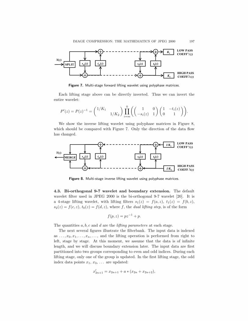
IMAGE COMPRESSION: THE MATHEMATICS OF JPEG 2000 197
X(z)
LOW PASS
COEFF (z)
HIGH PASS
COEFF (z)+
sm
(z)
+
SPLIT tm
(z)
+
s0(z)
+
t0(z)
K1
K2
γ
λ
Figure 7. Multi-stage forward lifting wavelet using polyphase matrices.
Each lifting stage above can be directly inverted. Thus we can invert theentire wavelet:
P ′(z) = P (z)−1 =(
1/K1
1/K2
) 0∏
i=m
((1 0
−si(z) 1
)(1 −ti(z)0 1
)).
We show the inverse lifting wavelet using polyphase matrices in Figure 8,which should be compared with Figure 7. Only the direction of the data flowhas changed.
Y(z)
LOW PASS
COEFF (z)
HIGH PASS
COEFF (z)+
sm
(z)
+
MERGE tm
(z)
+
s0(z)
+
t0(z)
1/K1
1/K2
γ
λ
Figure 8. Multi-stage inverse lifting wavelet using polyphase matrices.
4.3. Bi-orthogonal 9-7 wavelet and boundary extension. The defaultwavelet filter used in JPEG 2000 is the bi-orthogonal 9-7 wavelet [20]. It isa 4-stage lifting wavelet, with lifting filters s1(z) = f(a, z), t1(z) = f(b, z),s2(z) = f(c, z), t0(z) = f(d, z), where f , the dual lifting step, is of the form
f(p, z) = pz−1 + p.
The quantities a, b, c and d are the lifting parameters at each stage.The next several figures illustrate the filterbank. The input data is indexed
as . . . , x0, x1, . . . , xn, . . . , and the lifting operation is performed from right toleft, stage by stage. At this moment, we assume that the data is of infinitelength, and we will discuss boundary extension later. The input data are firstpartitioned into two groups corresponding to even and odd indices. During eachlifting stage, only one of the group is updated. In the first lifting stage, the oddindex data points x1, x3, . . . are updated:
x′2n+1 = x2n+1 + a ∗ (x2n + x2n+2),

198 JIN LI
where a and x′2n+1 are respectively the first stage lifting parameter and outcome.The entire operation corresponds to the filter s1(z) represented in Figure 8. Thecircle in Figure 9 illustrates one such operation performed on x1.
a=-1.586
b=-0.052
c= 0.883
d= 0.444
H0
H1
H2
H3
a
a
a
a
b
b
b
c
c
c
c
d
d
d
a
a
a
a
b
b
b
b
c
c
c
c
d
d
d
d
b d
High LowOriginal
x0
x1
x2
x3
x4
x5
x6
x7
x8
L0
L1
L2
L3
L4
a
a1
saved in its own position
Y = (x0+x
2)*a + x
1
x0
x1
x2
.
.
.
.
.
.
Figure 9. Bi-orthogonal 9-7 wavelet.
The second stage lifting, which corresponds to the filter t1(z) in Figure 8,updates the data at even indices:
x′′2n = x2n + b ∗ (x′2n−1 + x′2n+1),
where b and x′′2n are the second stage lifting parameter and output. The thirdand fourth stage lifting can be performed similarly:
Hn = x′2n+1 + c ∗ (x′′2n + x′′2n+2),
Ln = x′′2n + d ∗ (Hn−1 + Hn),
where Hn and Ln are the resultant high and low-pass coefficients. The value ofthe lifting parameters a, b, c, d are shown in Figure 9.
As illustrated in Figure 10, we may invert the dataflow, and derive an inverselifting of the 9-7 bi-orthogonal wavelet.
Since the actual data in an image transform is finite in length, boundary ex-tension is a crucial part of every wavelet decomposition scheme. For a symmetricodd-tap filter (the bi-orthogonal 9-7 wavelet falls into this category), symmetricboundary extension can be used. The data are reflected symmetrically alongthe boundary, with the boundary points themselves not involved in the reflec-tion. An example boundary extension with four data points x0, x1, x2 and x3

IMAGE COMPRESSION: THE MATHEMATICS OF JPEG 2000 199
a
a
a
a
b
b
b
c
c
c
c
d
d
d
a
a
a
a
b
b
b
b
c
c
c
c
d
d
d
d
b d
High LowOriginal
x0
x1
x2
x3
x4
x5
x6
x7
x8
L0
H0
L1
H1
L2
H2
L3
H3
L4
cd
d
L
X
R
Y
Y = X + ( L + R ) * d
X = Y + ( L + R ) * ( - d )
TRANSFORM
-d
-d
-d
-d
-c
-c
-c
-b
-b
-b
-b
-a
-a
-a
-d
-d
-d
-c
-c
-c -b
-a
-a
-c -a
-d -c -a
-a-b
-b
-b
INVERSE TRANSFORM
Original
.
.
.
.
.
.
INVERSE
DATA FLOW
Figure 10. Forward and inverse lifting (9-7 bi-orthogonal wavelet).
is shown in Figure 11. Because both the extended data and the lifting struc-ture are symmetric, all the intermediate and final results of the lifting are alsosymmetric with respect to the boundary points. Using this observation, it issufficient to double the lifting parameters of the branches that are pointing to-ward the boundary, as shown in the middle of Figure 11. Thus, the boundaryextension can be performed without additional computational complexity. Theinverse lifting can again be derived by inverting the dataflow, as shown in theright of Figure 11. Again, the parameters for branches that are pointing towardthe boundary points are doubled.
a b c d
a
a
b
b c
a
a b c
a
a
a
b
b
b
c
c
c
d
d
d
x0
x1
x2
x3
x2
x2
x1
x2
x3
x1
x0
a b
a
a
a
2a
2b
b
b
c
c
2c
2d
d
d
x0
x1
x2
x3
L0
H0
L1
H1
L0
H0
L1
H1
-2d
-d
-d
-c
-c
-2c -b
-a
-2a
-a-b
-2b
INVERSE TRANSFORM
x0
x1
x2
x3
FORWARD TRANSFORM
Figure 11. Symmetric boundary extension of bi-orthogonal 9-7 wavelet on 4
data points.

200 JIN LI
4.4. Two-dimensional wavelet transform. To apply a wavelet transformto an image we need to use a 2D version. In this case it is common to applythe wavelet transform separately in the horizontal and vertical directions. Thisapproach is called the separable 2D wavelet transform. It is possible to designa nonseparable 2D wavelet (see [32], for example), but this generally increasescomputational complexity with little additional coding gain. A sample one-scale separable 2D wavelet transform is shown in Figure 12. The 2D data arrayrepresenting the image is first filtered in the horizontal direction, which results intwo subbands: a horizontal low-pass and a horizontal high-pass subband. Thesesubbands are then passed through a vertical wavelet filter. The image is thusdecomposed into four subbands: LL (low-pass horizontal and vertical filter), LH(low-pass vertical and high-pass horizontal filter), HL (high-pass vertical and low-pass horizontal filter) and HH (high-pass horizontal and vertical filter). Sincethe wavelet transform is linear, we may switch the order of the horizontal andvertical filters yet still reach the same effect. By further decomposing subbandLL with another 2D wavelet (and iterating this procedure), we derive a multiscaledyadic wavelet pyramid. Recall that such a wavelet was illustrated in Figure 4.
G
H
2
x
a0
a1
2
G
H
2a00
a01
2
G
H
2a10
a11
2
Horizontal filtering Vertical filtering
Figure 12. A single scale 2D wavelet transform.
4.5. Line-based lifting. A trick in implementing the 2D wavelet transform isline-based lifting, which avoids buffering the entire 2D image during the verticalwavelet lifting operation. The concept can be shown in Figure 13, which is verysimilar to Figure 9, except that here each circle represents an entire line (row)of the image. Instead of performing the lifting stage by stage, as in Figure 9,line-based lifting computes the vertical low- and high-pass lifting, one line at atime. The operation can be described as follows:
Step 1: Initialization, phase 1. Three lines of coefficients x0, x1 and x2 are pro-cessed. Two lines of lifting operations are performed, and intermediate resultsx′1 and x′′0 are generated.

IMAGE COMPRESSION: THE MATHEMATICS OF JPEG 2000 201
High LowOriginal
x0
x1
x2
x3
x4
x5
x6
x7
x8
L0
H0
L1
H1
L2
H2
L3
H3
L4
1st
Lift
2nd
Lift
STEP2
STEP3
. . .
STEP1
Figure 13. Line-based lifting wavelet (bi-orthogonal 9-7 wavelet).
Step 2: Initialization, phase 2. Two additional lines of coefficients x3 andx4 areprocessed. Four lines of lifting operations are performed. The outcomes arethe intermediate results x′3 and x′′4 , and the first line of low and high-passcoefficients L0 and H0.
Step 3: Repeated processing. During the normal operation, the line based lift-ing module reads in two lines of coefficients, performs four lines of liftingoperations, and generates one line of low and high-pass coefficients.
Step 4: Flushing. When the bottom of the image is reached, symmetrical bound-ary extension is performed to correctly generate the final low and high-passcoefficients.
For the 9-7 bi-orthogonal wavelet, with line-based lifting, only six lines of workingmemory are required to perform the 2D lifting operation. By eliminating theneed to buffer the entire image during the vertical wavelet lifting operation, thecost to implement 2D wavelet transform can be greatly reduced
5. Quantization and Partitioning
After the wavelet transform, all wavelet coefficients are uniformly quantizedaccording to the rule
wm,n = sign sm,n
⌊ |sm,n|δ
⌋,
where sm,n is the transform coefficient, wm,n is the quantization result, δ is thequantization step size, sign(x) returns the sign of coefficient x, and b c is thefloor function. The effect of quantization is demonstrated in Figure 14.

202 JIN LI
TRANSFORM COEFF
4123, -12.4, -96.7, 4.5, �QUANTIZE COEFF(Q=1)
4123, -12, -96, 4, �
Figure 14. Effect of quantization.
The quantization process of JPEG 2000 is very similar to that of a conven-tional coder such as JPEG. However, the functionality is very different. In aconventional coder, since the quantization result is losslessly encoded, the quan-tization process determines the allowable distortion of the transform coefficients.In JPEG 2000, the quantized coefficients are lossy encoded through an embed-ded coder, thus additional distortion can be introduced in the entropy codingsteps. Thus, the main functionality of the quantization module is to map thecoefficients from floating representation into integer so that they can be moreefficiently processed by the entropy coding module. The image coding quality isnot determined by the quantization step size δ but by the subsequent bitstreamassembler. The default quantization step size in JPEG 2000 is rather fine, e.g.,δ = 1
128 .The quantized coefficients are then partitioned into packets. Each subband is
divided into non-overlapping rectangles of equal size, as described above, thismeans three rectangles corresponding to the subbands HL, LH, HH of eachresolution level. The packet partition provides spatial locality as it containsinformation needed for decoding image of a certain spatial region at a certainresolution.
The packets are further divided into non-overlapping rectangular code-blocks,which are the fundamental entities in the entropy coding operation. By applyingthe entropy coder to relatively small code-blocks, the original and working dataof the entire code-blocks can reside in the cache of the CPU during the entropycoding operation. This greatly improves the encoding and decoding speed. InJPEG 2000, the default size of a code-block is 64× 64. A sample partition andcode-blocks are shown in Figure 15. We mark the partition with solid thicklines. The partition contains quantized coefficients at spatial location (128, 128)
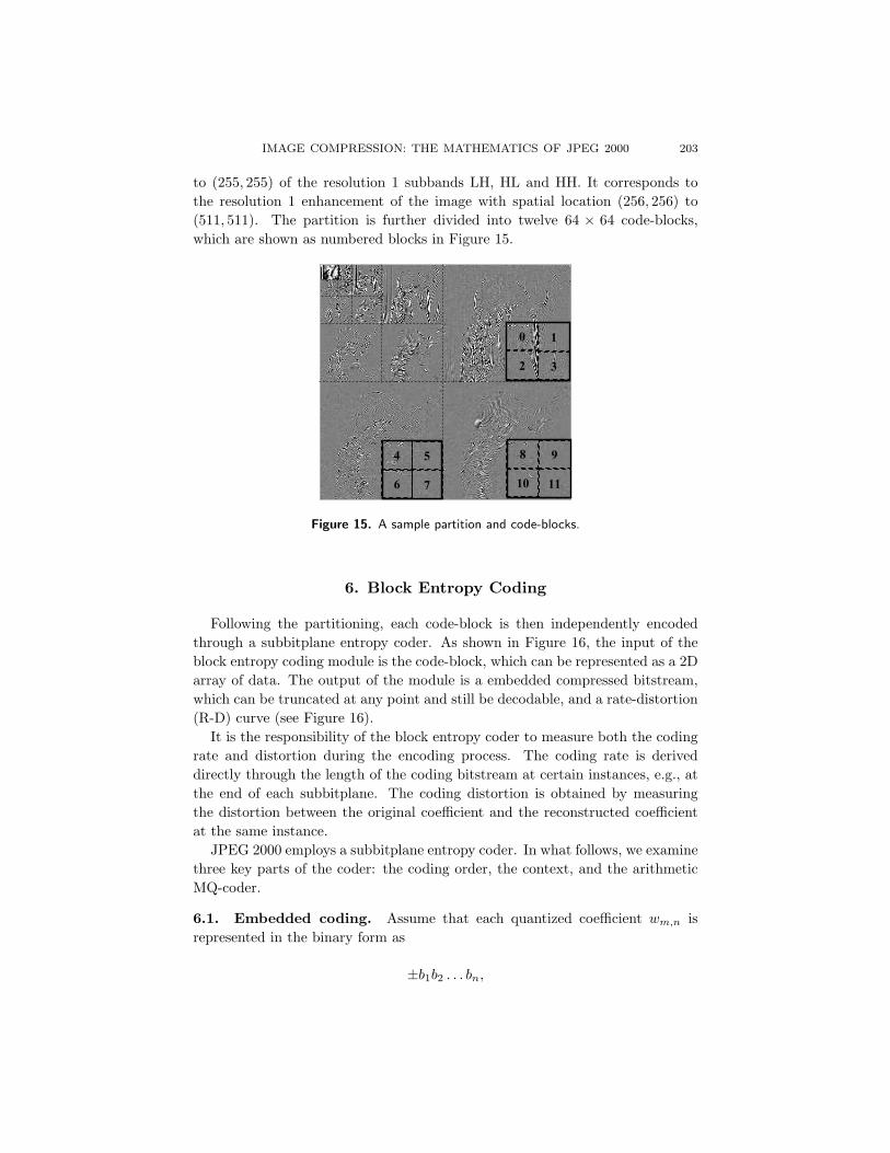
IMAGE COMPRESSION: THE MATHEMATICS OF JPEG 2000 203
to (255, 255) of the resolution 1 subbands LH, HL and HH. It corresponds tothe resolution 1 enhancement of the image with spatial location (256, 256) to(511, 511). The partition is further divided into twelve 64 × 64 code-blocks,which are shown as numbered blocks in Figure 15.
0 1
2 3
8 9
10 11
4 5
6 7
Figure 15. A sample partition and code-blocks.
6. Block Entropy Coding
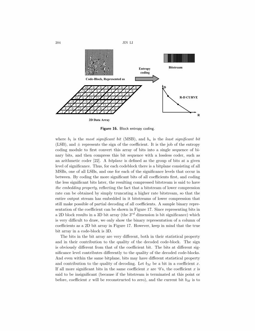
Following the partitioning, each code-block is then independently encodedthrough a subbitplane entropy coder. As shown in Figure 16, the input of theblock entropy coding module is the code-block, which can be represented as a 2Darray of data. The output of the module is a embedded compressed bitstream,which can be truncated at any point and still be decodable, and a rate-distortion(R-D) curve (see Figure 16).
It is the responsibility of the block entropy coder to measure both the codingrate and distortion during the encoding process. The coding rate is deriveddirectly through the length of the coding bitstream at certain instances, e.g., atthe end of each subbitplane. The coding distortion is obtained by measuringthe distortion between the original coefficient and the reconstructed coefficientat the same instance.
JPEG 2000 employs a subbitplane entropy coder. In what follows, we examinethree key parts of the coder: the coding order, the context, and the arithmeticMQ-coder.
6.1. Embedded coding. Assume that each quantized coefficient wm,n isrepresented in the binary form as
±b1b2 . . . bn,
204 JIN LI
45 0 0 0
-74 -13 0 0
21 0 4 0
14 0 23 23
0 0 0 0
3 0 4 0
0 3 5 0
0 0 0 0
0 1 -1 0
-4 33 0 -1
0 0 1 0
0 0 0 0
-4 5 0 0
-18 0 0 19
4 0 23 0
-1 0 0 0
Bitstream
D
R
R-D CURVE
Code-Block, Represented as
2D Data Array
Entropy
coding
Figure 16. Block entropy coding.
where b1 is the most significant bit (MSB), and bn is the least significant bit(LSB), and ± represents the sign of the coefficient. It is the job of the entropycoding module to first convert this array of bits into a single sequence of bi-nary bits, and then compress this bit sequence with a lossless coder, such asan arithmetic coder [22]. A bitplane is defined as the group of bits at a givenlevel of significance. Thus, for each codeblock there is a bitplane consisting of allMSBs, one of all LSBs, and one for each of the significance levels that occur inbetween. By coding the more significant bits of all coefficients first, and codingthe less significant bits later, the resulting compressed bitstream is said to havethe embedding property, reflecting the fact that a bitstream of lower compressionrate can be obtained by simply truncating a higher rate bitstream, so that theentire output stream has embedded in it bitstreams of lower compression thatstill make possible of partial decoding of all coefficients. A sample binary repre-sentation of the coefficient can be shown in Figure 17. Since representing bits ina 2D block results in a 3D bit array (the 3rd dimension is bit significance) whichis very difficult to draw, we only show the binary representation of a column ofcoefficients as a 2D bit array in Figure 17. However, keep in mind that the truebit array in a code-block is 3D.
The bits in the bit array are very different, both in their statistical propertyand in their contribution to the quality of the decoded code-block. The signis obviously different from that of the coefficient bit. The bits at different sig-nificance level contributes differently to the quality of the decoded code-blocks.And even within the same bitplane, bits may have different statistical propertyand contribution to the quality of decoding. Let bM be a bit in a coefficient x.If all more significant bits in the same coefficient x are ‘0’s, the coefficient x issaid to be insignificant (because if the bitstream is terminated at this point orbefore, coefficient x will be reconstructed to zero), and the current bit bM is to

IMAGE COMPRESSION: THE MATHEMATICS OF JPEG 2000 205
45 0 0 0
-74 -13 0 0
21 0 4 0
14 0 23 23
0 0 0 0
3 0 4 0
0 3 5 0
0 0 0 0
0 1 -1 0
-4 33 0 -1
0 0 1 0
0 0 0 0
-4 5 0 0
-18 0 0 19
4 0 23 0
-1 0 0 0
0 1 0 1 1 0 10 1 0 1 1 0 1 +
1 0 0 1 0 1 0 -
0 0 1 0 1 0 1 +
0 0 0 1 1 1 0 +
0 0 0 0 1 0 0 -
0 0 1 0 0 1 0 -
0 0 0 0 1 0 0 +
0 0 0 0 0 0 1 -
SIGNb1b2b3b4b5b6b7
w0
w1
w2
w3
w4
w5
w6
w7
ON
E L
IN
E O
F C
OE
F
45
-74
21
14
-4
-18
4
-1
Figure 17. Coefficients and binary representation.
be encoded in the mode of significance identification. Otherwise, the coefficientis said to be significant, and the bit bM is to be encoded in the mode of refine-ment. Depending on the sign of the coefficient, the coefficient can be positivesignificant or negative significant. We distinguish between significance identifi-cation and refinement bits because the significance identification bit has a veryhigh probability of being 0, and the refinement bit is usually equally distributedbetween 0 and 1. The sign of the coefficient needs to be encoded immediatelyafter the coefficient turns significant, i.e., a first non-zero bit in the coefficient isencoded. For the bit array in Figure 17, the significance identification and therefinement bits are shown with different shades in Figure 18.
0 1 0 1 1 0 10 1 +
1 0 0 1 0 1 0 -
0 0 1 0 1 0 1 +
0 0 0 1 1 1 0 +
0 0 0 0 1 0 0 -
0 0 1 0 0 1 0 -
0 0 0 0 1 0 0 +
0 0 0 0 0 0 1 -
SIGNb6
b5
b4
b3
b2
b1
b0
w0
w1
w2
w3
w4
w5
w6
w7
45
-74
21
14
-4
-18
4
-1
SIGNIFICANT
IDENTIFICATIONREFINEMENT
PREDICTED
INSIGNIFICANCE(PN)
PREDICTED
SIGNIFICANCE(PS)
REFINEMENT (REF)
Figure 18. Embedded coding of bit array.

206 JIN LI
6.2. Context. It has been pointed out [14; 21] that the statistics of significantidentification bits, refinement bits, and signs can vary tremendously. For exam-ple, if a quantized coefficientxi,j is of large magnitude, its neighbor coefficientsmay be of large magnitude as well. This is because a large coefficient locates ananomaly (e.g., a sharp edge) in the smooth signal, and such an anomaly usuallycauses a cluster of large wavelet coefficients in the neighborhood as well. Toaccount for such statistical variation, we entropy encode the significant identifi-cation bits, refinement bits and signs with context, each of which is a numberderived from already coded coefficients in the neighborhood of the current co-efficient. The bit array that represents the data is thus turned into a sequenceof bit-context pairs, as shown in Figure 19, which is subsequently encoded by acontext adaptive entropy coder. In the bit-context pair, it is the bit informationthat is actually encoded. The context associated with the bit is determined fromthe already encoded information. It can be derived by the encoder and the de-coder alike, provided both use the same rule to generate the context. Bits in thesame context are considered to have similar statistical properties, so that theentropy coder can measure the probability distribution within each context andefficiently compress the bits.
45 0 0 0
-74 -13 0 0
21 0 4 0
14 0 23 23
0 0 0 0
3 0 4 0
0 3 5 0
0 0 0 0
0 1 -1 0
-4 33 0 -1
0 0 1 0
0 0 0 0
-4 5 0 0
-18 0 0 19
4 0 23 0
-1 0 0 0
Bit: 0 1 1 0 0 0 0 0 0 1 0 0 0 0 0 0 0 0 0 ��
Ctx: 0 0 9 0 0 0 0 0 0 7 10 0 0 0 0 0 0 0 0 ��
Figure 19. Coding bits and contexts. The context is derived from information
from the already coded bits.
In the following, we describe the contexts that are used in the significantidentification, refinement and sign coding of JPEG 2000. For the rational ofthe context design, we refer to [2; 19]. Determining the context of significantidentification bit is a two-step process:
Step 1: Neighborhood statistics. For each bit of the coefficient, the number ofsignificant horizontal, vertical and diagonal neighbors are counted as h,vandd, as shown in Figure 20.
Step 2: Lookup table. According to the direction of the subband that the co-efficient is located (LH, HL, HH), the context of the encoding bit is indexed

IMAGE COMPRESSION: THE MATHEMATICS OF JPEG 2000 207
LH subband (also LL) HL subband HH subband(vertically high-pass) (horizontally high-pass) (diagonally high-pass)
h v d context h v d context d h + v context
2 x x 8 x 2 x 8 ≥3 x 81 ≥1 x 7 ≥1 1 x 7 2 ≥1 71 0 ≥1 6 0 1 ≥1 6 2 0 61 0 0 5 0 1 0 5 1 ≥2 50 2 x 4 2 0 x 4 1 1 40 1 x 3 1 0 x 3 1 0 30 0 ≥2 2 0 0 ≥2 2 0 ≥2 20 0 1 1 0 0 1 1 0 1 10 0 0 0 0 0 0 0 0 0 0
Table 1. Context for the significance identification coding.
through one of the three tables shown in Table 1. A total of nine context cate-gories are used for significance identification coding. The table lookup processreduces the number of contexts and enables probability of the statistics withineach context to be quickly obtained.
v
h
d
CURRENT
Figure 20. Number of significant neighbors: horizontal (h), vertical (v) and
diagonal (d).
To determine the context for sign coding, we calculate a horizontal sign counthand a vertical sign count v. The sign count takes a value of −1 if both hori-zontal/vertical coefficients are negative significant; or one coefficient is negativesignificant, and the other is insignificant. It takes a value of +1 if both hori-zontal/vertical coefficients are positive significant; or one coefficient is positivesignificant, and the other is insignificant. The value of the sign count is 0 if bothhorizontal/vertical coefficients are insignificant; or one coefficient is positive sig-nificant, and the other is negative significant.
With the horizontal and vertical sign count h and v, an expected sign and acontext for sign coding can then be calculated according to Table 2.
To calculate the context for the refinement bits, we measure if the currentrefinement bit is the first bit after significant identification, and if there is anysignificant coefficients in the immediate eight neighbors, i.e., h + v + d > 0. Thecontext for the refinement bit is tabulated in Table 3.

208 JIN LI
Sign countn
H − 1 −1 −1 0 0 0 1 1 1V − 1 0 1 −1 0 1 −1 0 1
Expected sign − − − − + + + + +Context 13 12 11 10 9 10 11 12 13
Table 2. Context and the expected sign for sign coding.
Context 14: Current refinement bit is the first bit after significant identifi-cation and there is no significant coefficient in the eight neighbors.
Context 15: Current refinement bit is the first bit after significant identifica-tion and there is at least one significant coefficient in the eight neighbors.
Context 16: Current refinement bit is at least two bits away from significantidentification.
Table 3. Context for the refinement bit.
6.3. MQ-coder: context dependent entropy coder. Through the afore-mentioned process, a data array is turned into a sequence of bit-context pairs, asshown in Figure 19. All bits associated with the same context are assumed to beindependently and identically distributed. Let the number of contexts be N , andlet there be ni bits in context i, within which the probability of the bits takingvalue 1 is pi. Using classic Shannon information theory [15; 16] the entropy ofsuch a bit-context sequence can be calculated as
H =N−1∑
i=0
ni
(−p log2 pi − (1− pi) log2(1− pi)). (6–1)
The task of the context entropy coder is thus to convert the sequence of bit-context pairs into a compact bitstream representation with length as close to theShannon limit as possible, as shown in Figure 21. Several coders are available forsuch task. The coder used in JPEG 2000 is the MQ-coder. In the following, wefocus the discussion on three key aspects of the MQ-coder: general arithmeticcoding theory, fixed point arithmetic implementation and probability estimation.For more details, we refer to [22; 23].
MQ-Coder
BITS
CTXBITSTREAM
Figure 21. Input and output of the MQ-coder.

IMAGE COMPRESSION: THE MATHEMATICS OF JPEG 2000 209
6.3.1. The Elias coder. The basic theory of the MQ-coder can be traced to theElias Coder [24], or recursive probability interval subdivision. Let S0S1S2 . . . Sn
be a series of binary bits that is sent to the arithmetic coder. Let Pi be theprobability that the bit Si be 1. We may form a binary representation (thecoding bitstream) of the original bit sequence by the following process:
Step 1: Initialization. Let the initial probability interval be (0, 1). We denotethe current probability interval as (C, C+A), where C is the bottom of theprobability interval, and A is the size of the interval. At the initialization, wehave C = 0 and A = 1.
Step 2: Probability interval subdivision. The binary symbols S0S1S2 . . . Sn areencoded sequentially. For each symbol Si, the probability interval (C, C+A) issubdivided into two sub-intervals
(C, C+A(1−Pi)
)and
(C+A(1−Pi), C+A
).
Depending on whether the symbol Si is 1, one of the two subintervals isselected: {
C ← C, A ← A(1− Pi), if Si = 0,C ← A(1− Pi), A ← APi, if Si = 1.
(6–2)
0
1
1-P0
P0
1-P1
P1 1-P2
P2
S0=0 S1=1 S2=0
0.100
Coding
result:
(Shortest binary
bitstream ensures that
interval
B=0.100 0000000 to
D=0.100 1111111 is
(B,D) A
)
AB
D
⊆
Figure 22. Probability interval subdivision.
Step 3: Bitstream output. Let the final coding bitstream be k1k2 . . . km, where m
is the compressed bitstream length. The final bitstream creates an uncertaintyinterval where the lower and upper bound can be determined as
Upperbound D = 0.k1k2 · · · km111 . . . ,
Lowerbound B = 0.k1k2 · · · km000 . . . .
As long as the uncertainty interval (B, D) is contained in the probability in-terval (C,C+A), the coding bitstream uniquely identifies the final probabilityinterval, and thus uniquely identifies each subdivision in the Elias coding pro-cess. The entire binary symbol strings S0S1S2 . . . Sn can thus be recoveredfrom the compressed representation. It can be shown that it is possible tofind a final coding bitstream with length
m ≤ d− log2 Ae+ 1

210 JIN LI
to represent the final probability interval (C, C+A). Notice that A is theprobability of the occurrence of the binary strings S0S1S2 . . . Sn, and theentropy of the original symbol stream can be calculated as
H =∑
S0S1···Sn
−A log2 A.
The arithmetic coder thus encodes the binary string within 2 bits of its entropylimit, no matter how long the symbol string is. This is very efficient.
6.3.2. The arithmetic coder: finite precision arithmetic operations. Exact im-plementation of Elias coding requires infinite precision arithmetic, an unrealisticassumption in real applications. Using finite precision, the arithmetic coder isdeveloped from Elias coding. Observing the fact that the coding interval A be-comes very small after a few operations, we may normalize the coding intervalparameter C and A as
C = 1.5 · [0.k1k2 · · · kL] + 2−L · 1.5 · Cx, A = 2−L · 1.5 ·Ax,
where L is a normalization factor determining the magnitude of the interval A,while Ax and Cx are fixed-point integers representing values between (0.75, 1.5)and (0, 1.5), respectively. Bits k1k2. . . km are the output bits that have alreadybeen determined (in reality, certain carryover operations have to be handledto derive the true output bitstream). By representing the probability intervalwith the normalization L and fixed-point integers Ax and Cx, it is possibleto use fixed-point arithmetic and normalization operations for the probabilityinterval subdivision operation. Moreover, since the value of Ax is close to 1.0,we may approximate Ax · Pi with Pi, the interval sub-division operation (6–2)calculated as
Cx = Cx,
Cx = C + Ax − Pi,
Ax = Ax − Pi,
Ax = Pi,
if Si = 0,
if Si = 1,
which can be done quickly without any multiplication. The compression perfor-mance suffers a little, as the coding interval now has to be approximated with afixed-point integer, and Ax · Pi is approximated with Pi. However, experimentsshow that the degradation in compression performance is less than three percent,which is well worth the saving in implementation complexity.
6.3.3. Probability estimation. In the arithmetic coder it is necessary to estimatethe probability Pi for each binary symbol Si to take the value 1. This is wherecontext comes into play. Within each context, it is assumed that the symbolsare independently identically distributed. We may then estimate the probabilityof the symbol within each context through observation of the past behaviors ofsymbols in the same context. For example, if we observe ni symbols in context

IMAGE COMPRESSION: THE MATHEMATICS OF JPEG 2000 211
i, with oi symbols to be 1, we may estimate the probability that a symbol takeson the value 1 in context i through Bayesian estimation as
Pi =oi + 1ni + 2
.
In the MQ-coder [22], probability estimation is implemented through a state-transition machine. It may estimate the probability of the context more effi-ciently, and may take into consideration the non-stationary characteristic of thesymbol string. Nevertheless, the principle is still to estimate the probabilitybased on past behavior of the symbols in the same context.
6.4. Coding order: subbitplane entropy coder. In JPEG 2000, becausethe embedded bitstream of a code-block may be truncated, the coding order,which is the order that the data array is turned into bit-context pair sequence,is of paramount importance. A sub-optimal coding order may allow importantinformation to be lost after the coding bitstream is truncated, and lead to severecoding distortion. It turns out that the optimal coding order first encodes thosebits with the steepest rate-distortion slope, which is defined as the coding dis-tortion decrease per bit spent [21]. Just as the statistical properties of the bitsare different in the bit array, their contribution of the coding distortion decreaseper bit is also different.
Consider a bit bi in the i-th most significant bitplane, where there are a totalof n bitplanes. If the bit is a refinement bit, then previous to the coding ofthe bit, the uncertainty interval of the coefficient is (A,A+2n−i). After therefinement bit has been encoded, the coefficient lies either in (A, A+2n−i−1) orin (A+2n−i, A+2n−i−1). If we further assume that the value of the coefficient isuniformly distributed in the uncertainty interval, we may calculate the expecteddistortion before and after the coding as
Dpre,REF =∫ A+2n−i
A
(x−A− 2n−i−1)2 dx = 112 4n−i,
Dpost,REF = 112 4n−i−1.
Since the value of the coefficient is uniformly distributed in the uncertaintyinterval, the probability for the refinement bit to take the values 0 and 1 is equal,thus, the coding rate of the refinement bit is:
RREF = H(bi) = 1 bit. (6–3)
The rate-distortion slope of the refinement bit at the i-th most significantbitplane is thus:
sREF(i) =Dprev,REF −Dpost,REF
RREF=
112 4n−i − 1
12 4n−i−1
1= 4n−i−2 (6–4)
In the same way, we may calculate the expected distortion decrease and codingrate for a significant identification bit at the i-th most significant bitplane. Before

212 JIN LI
the coding of the bit, the uncertainty interval of the coefficient ranges from −2n−i
to 2n−i. After the bit has been encoded, if the coefficient becomes significant,it lies in (−2n−i, −2n−i−1) or (+2n−i−1, +2n−i) depending on the sign of thecoefficient. If the coefficient is still insignificant, it lies in (−2n−i−1, 2n−i−1). Wenote that if the coefficient is still insignificant, the reconstructed coefficient beforeand after coding both will be 0, which leads to no distortion decrease (codingimprovement). The coding distortion only decreases if the coefficient becomessignificant. Assuming the probability that the coefficient becomes significant isp, and the coefficient is uniformly distributed within the significance interval(−2n−i, −2n−i−1) or (+2n−i−1, +2n−i), we may calculate the expected codingdistortion decrease as
Dprev,SIG −Dpost,SIG = p94
4n−i (6–5)
The entropy of the significant identification bit can be calculated as
RSIG = −(1− p) log2(1− p)− p log2 p + p · 1 = p + H(p),
where H(p) = −(1− p) log2(1− p)− p log2 p is the entropy of the binary symbolwith the probability of 1 being p. In (6–5), we account for the one bit which isneeded to encode the sign of the coefficient if it becomes significant.
We may then derive the expected rate-distortion slope for the significanceidentification bit coding as
sSIG(i) =Dprev,SIG −Dpost,SIG
RSIG=
91 + H(p)/p
4n−i−2
From this and (6–4), we arrive at the following conclusions:
Conclusion 1. The more significant bitplane that the bit is located, the earlierit should be encoded.
A key observation is, within the same coding category (significance identifi-cation/refinement), one more significance bitplane translates into 4 times morecontribution in distortion decrease per coding bit spent. Therefore, the code-block should be encoded bitplane by bitplane.
Conclusion 2. Within the same bitplane, we should first encode the significanceidentification bit with a higher probability of significance.
It can be shown that the function H(p)/p increases monotonically as theprobability of significance decreases. As a result, the higher probability of sig-nificance, the higher contribution of distortion decrease per coding bit spent.
Conclusion 3. Within the same bitplane, the significance identification bitshould be encoded earlier than the refinement bit if the probability of significanceis higher than 0.01.

IMAGE COMPRESSION: THE MATHEMATICS OF JPEG 2000 213
It is observed that the insignificant coefficients with no significant coefficientsin its neighborhood usually have a probability of significance below 0.01, whileinsignificant coefficients with at least one significant neighbor usually have ahigher probability of significance.
As a result of these three conlusions, the entropy coder in JPEG 2000 en-codes the code-block bitplane by bitplane, from the most significant bitplane tothe least significant bitplane; and within each bitplane, the bit array is furtherordered into three subbitplanes: the predicted significance (PS), the refinement(REF) and the predicted insignificance (PN).
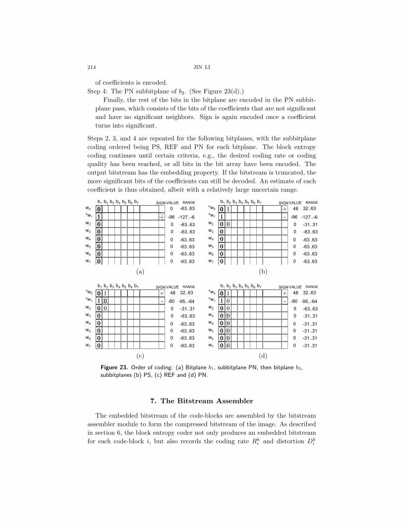
Using the data array in Figure 23 as an example, we illustrate the block codingorder of JPEG 2000 with a series of sub-figures in Figure 23. Each sub-figureshows the coding of one subbitplane. The block coding order of JPEG 2000 isas follows:
Step 1: The most significant bitplane, the PN subbitplane of b1. (See Fig-ure 23(a).)
First, the most significant bitplane is examined and encoded. Since at first,all coefficients are insignificant, all bits in the MSB bitplane belong to the PNsubbitplane. Whenever a 1 bit is encountered (rendering the correspondingcoefficient non-zero) the sign of the coefficient is encoded immediately after-wards. With the information of those bits that have already been coded andthe signs of the significant coefficients, we may figure out an uncertain rangefor each coefficient. The reconstruction value of the coefficient can also beset, e.g., at the middle of the uncertainty range. The outcome of our sam-ple bit array after the coding of the most significant bitplane is shown inFigure 23(a). We show the uncertainty range and the reconstruction valueof each coefficient under columns “value” and “range” in the sub-figure, re-spectively. As the coding proceeds, the uncertainty range shrinks, and bringsbetter and better representation to each coefficient.
Step 2: The PS subbitplane of b2. (See Figure 23(b).)After all bits in the most significant bitplane have been encoded, the coding
proceeds to the PS subbitplane of the second most significant bitplane (b2).The PS subbitplane consists of bits of the coefficients that are not significant,but has at least one significant neighbor. The corresponding subbitplane cod-ing is shown in Figure 23(b). In this example, coefficients w0 and w2 are theneighbors of the significant coefficient w1, and they are encoded in this pass.Again, if a 1 bit is encountered, the coefficient becomes significant, and itssign is encoded right after. The uncertain ranges and reconstruction value ofthe coded coefficients are updated according to the newly coded information.
Step 3: The REF subbitplane of b2. (See Figure 23(c).)The coding then moves to the REF subbitplane, which consists of the
bits of the coefficients that are already significant in the past bitplane. Thesignificance status of the coefficients is not changed in this pass, and no sign
214 JIN LI
of coefficients is encoded.Step 4: The PN subbitplane of b2. (See Figure 23(d).)
Finally, the rest of the bits in the bitplane are encoded in the PN subbit-plane pass, which consists of the bits of the coefficients that are not significantand have no significant neighbors. Sign is again encoded once a coefficientturns into significant.
Steps 2, 3, and 4 are repeated for the following bitplanes, with the subbitplanecoding ordered being PS, REF and PN for each bitplane. The block entropycoding continues until certain criteria, e.g., the desired coding rate or codingquality has been reached, or all bits in the bit array have been encoded. Theoutput bitstream has the embedding property. If the bitstream is truncated, themore significant bits of the coefficients can still be decoded. An estimate of eachcoefficient is thus obtained, albeit with a relatively large uncertain range.
0
1 -
0
0
0
0
0
0
SIGNb1b2b3b4b5b6b7
00
1 -
0
0
0
0
0
0
w0
*w1
w2
w3
w4
w5
w6
w7
VALUE
0
RANGE
-63..63
-96 -127..-64
-63..630
-63..630
-63..630
-63..630
-63..630
-63..630
0
1
0
0
0
0
0
0
+
SIGNb1b2b3b4b5b6b7
00 1 +
1 -
0 0
0
0
0
0
0
*w0
*w1
w2
w3
w4
w5
w6
w7
VALUE
48
RANGE
32..63
-96 -127..-64
-31..310
-63..630
-63..630
-63..630
-63..630
-63..630
(a) (b)
0
1
0
0
0
0
0
0
SIGNb1b2b3b4b5b6b7
00 1 +
1 0 -
0 0
0
0
0
0
0
*w0
*w1
w2
w3
w4
w5
w6
w7
VALUE
48
RANGE
32..63
-80 -95..-64
-31..310
-63..630
-63..630
-63..630
-63..630
-63..630
0
1
0
0
0
0
0
0
SIGNb1b2b3b4b5b6b7
00 1 +
1 0 -
0 0
0 0
0 0
0 0
0 0
0 0
*w0
*w1
w2
w3
w4
w5
w6
w7
VALUE
48
RANGE
32..63
-80 -95..-64
-63..630
-31..310
-31..310
-31..310
-31..310
-31..310
(c) (d)
Figure 23. Order of coding: (a) Bitplane b1, subbitplane PN, then bitplane b2,
subbitplanes (b) PS, (c) REF and (d) PN.
7. The Bitstream Assembler
The embedded bitstream of the code-blocks are assembled by the bitstreamassembler module to form the compressed bitstream of the image. As describedin section 6, the block entropy coder not only produces an embedded bitstreamfor each code-block i, but also records the coding rate Rk
i and distortion Dki

IMAGE COMPRESSION: THE MATHEMATICS OF JPEG 2000 215
at the end of each subbitplane, where k is the index of the subbitplane. Thebitstream assembler module determines how much bitstream of each code-blockis put to the final compressed bitstream. It determines a truncation point ni foreach code-block so that the distortion of the entire image is minimized upon arate constraint:
min∑
i
Dnii, with∑
i
Rnii ≤ B. (7–1)
Since there are a discrete number of truncation points ni, the constraint min-imization problem of equation (7–1) can be solved by distributing bits first tothe code-blocks with the steepest distortion per rate spent. The process of bitallocation and assembling can be performed as follows:
Step 1: Initialization. We initialize all truncation points to zero: ni = 0.Step 2: Incremental bit allocation. For each code block i, the maximum possible
gain of distortion decrease per rate spent is calculated as
Si = maxk>ni
Dnii −Dk
i
Rki −Rni
i
.
We call Si the rate-distortion slope of the code-block i. The code-blockwith the steepest rate-distortion slope is selected, and its truncation point isupdated as
nnewi = argk>ni
(Dnii−Dki
Rki −Rnii
= Si
).
A total of Rnnew
ii − Rni
i bits are sent to the output bitstream. This leads toa distortion decrease of Dni
i −Dnnew
ii . It can be easily proved that this is the
maximum distortion decrease achievable for spending Rnnew
ii −Rni
i bits.Step 3: Repeat Step 2 until the required coding rate B is reached.
The above optimization procedure does not take into account the last seg-ment problem, i.e., when the coding bits available is smaller than R
nnewi
i −Rnii
bits. However, in practice, usually the last segment is very small (within 100bytes), so that the residual sub-optimally is not a big concern.
Following exactly the optimization procedure above is computationally complex.The process can be speeded up by first calculating a convex hull of the R-D slopeof each code-block i, as follows:
Step 1: Set S to the set of all truncation points.Step 2: Set p to the first truncation point in S.Step 3: Do until p is the last truncation point in S:
(i) Set k to the next truncation point after p in S.
(ii) Set Ski =
Dpi −Dk
i
Rki −Rp
i
.

216 JIN LI
(iii) If p is not the first truncation point in S and Ski ≥ Sp
i , remove p from S
and move p back one truncation point in S; otherwise, set p = k.
(iv) [End of current iteration. Restart at step 3(i), unless p is the last trun-cation point in S.]
Once the R-D convex hull is calculated, the optimal R-D optimization becomessimply the search of a global R-D slope λ, where the truncation point of eachcode-block is determined by:
ni = arg maxk
(Sk
i > λ)
Putting the truncated bitstream of all code-blocks together, we obtain a com-pressed bitstream associated with each R-D slope λ. To reach a desired codingbitrate B, we just search the minimum λ whose associated bitstream satisfiesthe rate inequality (7–1). The R-D optimization procedure can be illustrated inFigure 24.
D1
R1
D2
R2
D3
R3
D4
R4
r1 r
2
r3
r4
. . .
r1
r2
r3
r4
Assembled bitstream:
Figure 24. Bitstream assembler: for each R-D slope λ, a truncation point can
be found at each code-block. The slope λ should be the minimum slope that
the allocated rate for all code-blocks is smaller than the required coding rate B.
To form a compressed image bitstream with progressive quality improvementproperty, so that we may gradually improve the quality of the received im-age as more and more bitstream arrives, we may design a series of rate points,B(1), B(2), . . . , B(n). A sample rate point set is 0.0625, 0.125, 0.25, 0.5, 1.0 and2.0 bpp (bit per pixel). For an image of size 512 × 512, this corresponds to acompressed bitstream size of 2k, 4k, 8k, 16k, 32k and 64k bytes. First, the globalR-D slope λ(1) for rate point B(1) is calculated. The first set of truncation point

IMAGE COMPRESSION: THE MATHEMATICS OF JPEG 2000 217
of each code-block n(1)i is thus derived. These bitstream segments of the code-
blocks of one resolution level at one spatial location is grouped into a packet. Allpackets that consist of the first segment bitstream form the first layer that rep-resents the first quality increment of the entire image at full resolution. Then,we may calculate the second global R-D slope λ(2) corresponding to the ratepoint B(2). The second truncation point of each code-block n
(2)i can be derived,
and the bitstream segment between the first n(1)i and the second n
(2)i truncation
points constitutes the second bitstream segment of the code-blocks. We againassemble the bitstream of the code-blocks into packets. All packets that consistof the second segment bitstreams of the code-blocks form the second layer of thecompressed image. The process is repeated until all n layers of bitstream areformed. The resultant JPEG 2000 compressed bitstream is thus generated andcan be illustrated with Figure 25.
Packet
Head BodyRe
syn
c
SO
T m
ark
er
SO
C m
ark
er
Glo
ba
l
He
ad
er
SO
S m
ark
er
Til
e H
ea
de
r
Packet
Head BodyRe
syn
c
SO
T m
ark
er
SO
S m
ark
er
Til
e H
ea
de
r
EO
I m
ark
er
extra tiles
Packet
Head BodyRe
syn
c
Packet
Head BodyRe
syn
c
Layer n
Layer 1
.
.
.
Figure 25. JPEG 2000 bitstream syntax. SOC = start of image (codestream)
marker; SOT = start of tile marker; SOS = start of scan marker; EOI = end of
image marker.
8. The Performance of JPEG 2000
Finally, we briefly demonstrate the compression performance of JPEG 2000.We compare JPEG 2000 with the traditional JPEG standard. The test imageis the “Bike” standard image (gray, 2048 × 2560), shown in Figure 26. Threemodes of JPEG 2000 are tested, and are compared against two modes of JPEG.The JPEG modes are progressive (P-DCT) and sequential (S-DCT) both withoptimized Huffman tables [4]. The JPEG 2000 modes are single layer with thebi-orthogonal 9-7 wavelet (S-9,7), six layer progressive with the bi-orthogonal 9-7wavelet (P6-9,7), and 7 layer progressive with the (3,5) wavelet (P7-3,5). TheJPEG 2000 progressive modes have been optimized for 0.0625, 0.125, 0.25, 0.5,1.0, 2.0 bpp and lossless for the 5× 3 wavelet. The JPEG progressive mode uses

218 JIN LI
a combination of spectral refinement and successive approximation. We showthe performance comparison in Figure 27.
Figure 26. Original “Bike” test image.
JPEG 2000 results are significantly better than JPEG results for all modesand all bit-rates on this image. Typically JPEG 2000 provides only a few dBimprovement from 0.5 to 1.0 bpp but substantial improvement below 0.25 bppand above 1.5 bpp. Also, JPEG 2000 achieves scalability at almost no additional

IMAGE COMPRESSION: THE MATHEMATICS OF JPEG 2000 219
Figure 27. Performance comparison: JPEG 2000 versus JPEG. From [1], cour-
tesy of the authors, Marcellin et al.
cost. The progressive performance is almost as good as the single layer JPEG2000 without the progressive capability. The slight difference is due solely tothe increased signaling cost for the additional layers (which changes the packetheaders). It is possible to provide “generic rate scalability” by using upwards offifty layers. In this case the “scallops” in the progressive curve disappear, butthe overhead may be slightly increased.
References
[1] M. W. Marcellin, M. Gormish, A. Bilgin, M. P. Boliek, “An overview of JPEG2000”,pp. 523–544 in Proc. of the Data Compression Conference, Snowbird (UT), March2000.
[2] M. W. Marcellin and D. S. Taubman, Jpeg2000: Image Compression Fundamentals,Standards, and Practice, Kluwer International Series in Engineering and ComputerScience, Secs 642.
[3] ISO/IEC JTC1/SC29/WG1/N1646R, “JPEG 2000 Part I final committee draft,version 1.0”, March 2000, http://www.jpeg.org/public/fcd15444-1.pdf
[4] William B. Pennebaker, Joan L. Mitchell, Jpeg: Still image data compressionstandard, Kluwer Academic Publishers, September 1992.
[5] A. Zandi, J. D. Allen, E. L. Schwartz, and M. Boliek, “CREW: compression withreversible embedded wavelets”, pp. 212–221 in Proc. of IEEE Data CompressionConference, Snowbird (UT), March 1995.

220 JIN LI
[6] J. Shapiro, “Embedded image coding using zerotree of wavelet coefficients”, IEEETrans. Signal Processing 41 (1993), 3445–3462.
[7] S. Mallat, A wavelet tour of signal processing, Academic Press, 1998.
[8] I. Daubechies, Ten lectures on wavelets, second ed., SIAM, Philadelphia, 1992.
[9] C. S. Burrus, R. A. Gopinath and H. Guo, Introduction to wavelets and wavelettransforms, a primer, Prentice Hall, Upper Saddle River (NJ), 1998.
[10] I. Daubechies and W. Sweldens, “Factoring wavelet transforms into lifting steps”,J. Fourier Anal. Appl. 4:3 (1998).
[11] W. Sweldens, “Building your own wavelets at home”, in: Wavelets in ComputerGraphics, ACM SIGGRAPH Course Notes, 1996.
[12] C. Valen, “A really friendly guide to wavelets”, http://perso.wanadoo.fr/polyvalens/clemens/wavelets/wavelets.html.
[13] J. Li, P. Cheng, and J. Kuo, “On the improvements of embedded zerotreewavelet (EZW) coding”, pp. 1490–1501 in SPIE: Visual Communication and ImageProcessing, vol. 2501, Taipei, Taiwan, May 1995.
[14] M. Boliek, “New work item proposal: JPEG 2000 image coding system”, ISO/IECJTC1/SC29/WG1 N390, June 1996.
[15] T. M. Cover and J. A. Thomas, Elements of Information Theory, Wiley, NewYork, 1991.
[16] T. M. Cover and J. A. Thomas, “Elements of information theory: online resources”,http://www-isl.stanford.edu/̃ jat/eit2/index.shtml.
[17] ISO/IEC JTC1/SC29/WG1 N505, “Call for contributions for JPEG 2000 (ITC1.29.14, 15444): image coding system”, March 1997.
[18] J. H. Kasner, M. W. Marcellin and B. R. Hunt, “Universal trellis coded quantiza-tion”, IEEE Trans. Image Processing 8:12 (Dec. 1999), 1677–1687.
[19] D. Taubman, “High performance scalable image compression with EBCOT”, IEEETrans. Image Processing 9:7 (July 2000), 1158–1170.
[20] M. Antonini, M. Barlaud, P. Mathieu and I. Daubechies, “Image coding usingwavelet transform”, IEEE Trans. Image Processing, 1:2 (Apr. 1992), 205–220.
[21] J. Li and S. Lei, “An embedded still image coder with rate-distortion optimiza-tion”, IEEE Trans. Image Processing 8:7 (July 1999), 913–924.
[22] ISO/IEC JTC1/SC29/WG1 N1359, “Information technology— coded representa-tion of picture and audio information— lossy/lossless coding of bi-level images”,14492 Final Committee Draft, July 1999.
[23] W. Pennebaker, J. Mitchell, G. Langdon, and R. Arps, “An overview of the basicprinciples of the q-coder adaptive binary arithmetic coder”, IBM J. Res. Develop32:6 (1988), 717–726.
[24] Ian H. Witten, Radford M. Neal, and John G. Cleary, “Arithmetic coding for datacompression,” Communications of the ACM 30:6 (1987), 520–540.
[25] J. Li and H. Sun, “A virtual media (Vmedia) interactive image browser”, IEEETrans. Multimedia, Sept. 2003.
[26] K. R. Rao and P. Yip, Rao, “Discrete cosine transform: algorithms, advantages,applications”. Academic Press, Boston, 1990.

IMAGE COMPRESSION: THE MATHEMATICS OF JPEG 2000 221
[27] S. Mallat, A wavelet tour of signal processing, Academic Press, 1998.
[28] P. P. Vaidyanathan, Multirate systems and filter banks, Prentice-Hall, EnglewoodCliffs (NJ), 1993.
[29] R. Gonzalez and R. Woods, Digital image processing, Addison-Wesley, Reading(MA), 1992.
[30] K. R. Rao and D. F. Elliott, Fast transforms: algorithms, analyses and applications,Academic Press, New York, 1982.
[31] R. Rosenholtz and A. B. Watson, “Perceptual adaptive JPEG coding”, pp. 901–904in Proc. IEEE International Conference on Image Processing, Lausanne, Switzer-land, 1994.
[32] G. V. Auwera, A. Munteanu, and J. Cornelis, “Evaluation of a quincunx waveletfilter design approach for quadtree-based embedded image coding”, pp. 190–194 inProc. of the IEEE International Conference on Image Processing (ICIP), Vancouver,Canada, Sept. 2000.
Jin LiMicrosoft ResearchCommunication Collaboration and Signal ProcessingOne Microsoft Way, Bld. 113/3161Redmond, WA 98052