UNIVERSITY OF CALIFORNIA, SAN DIEGO

Image based physiological noise correction for perfusion-based functional MRI

A thesis submitted in partial satisfaction of the requirements for the degree Master of Science

in

Bioengineering

By

Khaled Restom

Committee in charge: Professor Thomas T. Liu, Chair Professor Andrew D. McCulloch, Co-Chair Professor Richard B. Buxton

2004

Copyright

Khaled S Restom, 2004

All rights reserved.

The Thesis of Khaled Restom is approved by:

University of California, San Diego

2004

DEDICATION

This thesis is dedicated to…..

TABLE OF CONTENTS

Signature Page Dedication Table of Contents List of Abbreviations List of Figures List of Tables Preface Acknowledgements Abstract 1. Introduction 2. Theory 3. Methods 4. Results 5. Discussion 6. Future perspectives Appendix A: Tables Appendix B: Figures References

LIST OF ABBREVIATIONS

ASL: Arterial Spin Labeling BOLD: Blood Oxygenation Level Dependent fMRI: Functional Magnetic Resonance Imaging GLM: General Linear Model TR: Repetition Time CC: Correlation Coefficient SNR: Signal to Noise Ratio NMR: Nuclear Magnetic Resonance CBV: Cerebral Blood Volume CBF: Cerebral Blood Flow TE: Echo Time FOV: Field of View CMRO2: Cerebral metabolic rate of oxygen EPI: Echo Planar Imaging

LIST OF FIGURES

Figure 1: Pixel signal model Figure 2: A simplified model of an ASL experiment Figure 3: Example showing calculation of cardiac phase Figure 4: Example showing calculation respiratory phase Figure 5: Example data showing estimated cardiac and respiratory components Figure 6: Spatial power in BOLD images (TR 250ms) centered around respiratory

peak Figure 7: Spatial power in BOLD images (TR 250ms) centered around cardiac peak Figure 8: Fourier spectra of a single voxel (BOLD, TR 250ms) Figure 9: Example of a resting state time series (BOLD, TR 250ms) Figure 10: Spatial power in BOLD images (TR 2000ms) centered around respiratory Figure 11: Fourier spectra of a single voxel (BOLD, TR 200ms) Figure 12: Example of a resting state time series (BOLD, TR 200ms) Figure 13: F statistic versus delay time (subject 1) Figure 14: F statistic versus delay time (all subjects) Figure 15: Average number of voxels across subject 1 that exhibit significant F

statistic Figure 16: Average number of voxels across all subjects that exhibit significant F

statistic Figure 17: Example of a perfusion time series before and after correction Figure 18: Example of a correlation map overlaid on an average perfusion map Figure 19: Summary of correlation statistics for all subjects

LIST OF TABLES

Table 1: Summary of physiological noise regressors ( ) and physiological noise parameters ( )

TOTP

TOTcTable 2: Summary of estimated delay times (∆) that were used with methods 3 and 4

ACKNOWLEDGEMENTS

Thomas T. Liu, PhD. Richard B. Buxton, PhD Larry Frank, PhD. Yashar Behzadi, M.S. Kamil Uludag, PhD Yousef Mazaheri, PhD. Wen-Chau Wu, PhD. Joanna Perthen, PhD.

ABSTRACT OF THE THESIS

Image based physiological noise correction for perfusion-based functional MRI

By

Khaled S Restom

Master of Science in Bioengineering

University of California, San Diego, 2004

Professor Thomas T. Liu, Chair

Professor Andrew D. McCulloch

Professor Richard B. Buxton

Physiological fluctuations are often a dominant source of noise in functional

magnetic resonance imaging (fMRI) experiments, especially at higher field strengths.

A number of methods have been developed for the reduction of physiological noise in

fMRI experiments. These include image based retrospective correction

(RETROICOR), k-space based retrospective correction, and navigator echo based

correction. At present the application of these methods has been focused primarily on

experiments using blood oxygenation level-dependent contrast. Perfusion-based fMRI

using arterial spin labeling (ASL) is becoming increasing popular because of its

potential to better localize functional activation to the sites of neuronal activity. Thus,

in this thesis we investigate four extensions of RETROICOR to ASL. While

significant improvement in statistical power was observed for each method, we found

the greatest improvement resulted when 1) physiological noise is estimated separately

for tag and control images and 2) the contribution of physiological fluctuations during

the tagging process to noise in the tag images is included.

1. INTRODUCTION

Physiological fluctuations are often a dominant source of noise in functional

magnetic resonance imaging (fMRI) experiments, especially at higher field strengths

{Turner, Jezzard et al. 1993}. Physiological noise in fMRI is manifested as inter-

image variation. Since this variance can be on the order of the signal of interest,

statistical sensitivity to functional activity can be reduced. Cardiac and respiratory

activity have been shown to be the primary sources of physiological noise. Due to the

complexity of brain physiology, understanding the contribution of physiological

activity to brain imaging remains a challenge.

Cardiac related image intensity fluctuation can be caused by pulsatility of blood

flow in the brain, which can result in vessel pulsation, cerebral spinal movement, and

tissue deformation. Investigations into the properties of cardiac noise have found that

it is largely localized in the brain in regions that are near vessels {Dagli, Ingeholm et

al. 1999}. Since MRI is a measure of the magnetization of the imaged tissue, inflow

of blood can introduce signal perturbations in parts of tissue near vessels. While this

mechanism may explain some of the cardiac related noise, a complete understanding

of these effects is lacking.

In addition, Magnetic field fluctuations that result from thoracic cavity expansion

and bulk head movement during respiration can also cause undesired image artifacts.

In contrast to cardiac related noise, respiratory noise has largely been shown to affect

the image globally {Noll and Schneider 1994}. However, localized inter-image

variations around the ventricles and brain edges have also been reported {Glover, Li et

al. 2000}.

A number of methods have been developed for the reduction of physiological

noise in fMRI experiments. These include image based retrospective correction

(RETROICOR) {Glover, Li et al. 2000}, k-space based retrospective correction

(RETROKCOR) {Hu, Le et al. 1995}, and navigator echo based correction {Pfeuffer,

Van de Moortele et al. 2002}. At present the application of these methods has been

focused primarily on experiments using blood oxygenation level dependent (BOLD)

contrast. However, perfusion-based fMRI using arterial spin labeling (ASL) is

becoming increasing popular because of its potential to better localize functional

activation to the sites of neuronal activity {Luh, Wong et al. 2000}. In this work we

investigate methods for the reduction of physiological noise in ASL experiments. We

begin by reviewing the current physiological noise correction methods.

1.1.1 RETROICOR

This method assumes that physiological noise induces fluctuation in the MR image

time series. Physiological data collected during the imaging sequence used to form a

low order Fourier series expansion with cardiac and respiratory phase terms. After the

coefficients of the Fourier series are determined by least squares for each pixel time

series, the modeled physiological noise is subtracted out. The resultant time exhibits

significantly reduced cardiac and respiratory noise {Glover, Li et al. 2000}.

1.1.2 RETROKCOR

This method employs the same basic concept as RETROICOR except that the

Fourier series is fit to data in the k-space time series, not image space {Hu, Le et al.

1995}. This method showed useful results in correcting respiratory induced effects.

However, this method is limited by signal to noise ratio (SNR) and since the SNR is

greatest at the center of k-space only time series data near the center of k-space can be

fit to the Fourier series. As a result, only low order spatial correction can be made

{Glover, Li et al. 2000}.

1.1.3 Navigator Methods

Navigator methods use information from an auxiliary echo and the center of k-

space of the image to quantify off resonance noise. This method was introduced by

Pfeuffer et al. as dynamic off-resonance in k-space (DORK) correction {Pfeuffer, Van

de Moortele et al. 2002}. The DORK correction method reduces time varying zero

and first order phase shifts for EPI imaging. The method assumes that uniform (across

each slice) frequency and phase changes result from respiration (due to changes in the

magnetic field that cause NMR phase shifts). The phase information is acquired from

a navigator echo in addition to data at the center of k-space. Since this method only

samples a projection of the brain, it lacks the ability to localize the source of the noise.

As a result, its application can result in incomplete correction.

1.1.4 Estimation of Respiration induced Noise from undersampled multislice fMRI

data

Most fMRI experiments sample brain images at a sampling rate that is the less

than the Nyquist frequency for respiratory and cardiac fluctuations. As a result, it is

difficult to estimate the contribution of physiological fluctuations since any such

contribution will be aliased into lower frequencies. Aliased signals from higher

frequency signals can also overlap activity related signals, thereby making it difficult

to detect significant activation. The method introduced by Frank et al {Frank, Buxton

et al. 2001} uses multislice acquisition to critically sample respiratory induced noise.

By reordering the multislice image data using temporal rather than spatial ordering,

unaliased respiratory noise is estimated regardless of image repetition time (TR). For

example, if 8 slices were acquired in a TR of 2 seconds, the effective slice sampling

rate is (2 sec)/(8 slices) = 0.25 sec. Although the pixel time series is sampled at a 2 s

TR, reordering the slices temporally (in the order they were acquired) results in a

sampling rate that is high enough to sample physiological fluctuations. By detecting

global noise in the reordered image time series, this method has been shown to

significantly reduce respiratory related noise. However, since cardiac related noise is

more localized in the brain image, this method is less successful in reducing cardiac

related noise.

1.2 Application of physiological noise correction to ASL

Published reports of the application of the current physiological noise correction

schemes to ASL have been particularly limited. Among the reviewed correction

methods, only DORK has been explicitly used to correct respiratory induced noise in

perfusion fMRI image time series {Pfeuffer, Adriany et al. 2002}. However, a

comprehensive description of the application of DORK to ASL was not given.

In this work, we investigate the use of RETROICOR to correct physiological noise

in ASL images. Although we had the option to investigate the other reviewed

correction schemes, we chose RETROICOR because 1) it required no changes in the

MR imaging sequences whereas DORK requires a navigator echo, 2) it provided

significant correction of both cardiac and respiratory noise whereas the other

correction methods were unsuccessful at removing localized cardiac noise.

1.3 Outline of the thesis

In this thesis, we investigate the use of RETROICOR to correct physiological

noise in ASL images. We begin in section 2 with a description of the basics of BOLD

and ASL imaging. We then describe the BOLD and ASL general linear model

(GLM). Since our perfusion based noise correction methods are based on

RETROICOR, it is important that we achieve similar performance in noise correction

to that of published results. Consequently, we describe BOLD based physiological

noise correction. We then introduce four extensions of RETROICOR to estimate

cardiac and respiratory related noise in ASL.

Section 3, describes the imaging and physiological data collection methods. This

section will also cover how we assessed the performance of BOLD and ASL

correction of physiological noise. We accessed BOLD correction mainly by using

similar methods employed in {Glover, Li et al. 2000}, whereas ASL correction was

mainly assessed using the F statistic and correlation analysis.

Section 4 presents the results of BOLD and ASL correction of physiological noise.

The primary objective of showing the BOLD specific results will be to compare our

noise correction results to that of published results in {Glover, Li et al. 2000}. We

show that method 4 provided the best improvement in detecting functional perfusion

activity.

Section 5 summarizes the results of thesis and discusses the main findings. Finally

section 6 suggests area of future work.

Earlier versions of the work presented in this thesis have appeared in {Restom,

Behzadi et al. 2004}.

2. THEORY

2.1 BOLD Imaging

BOLD based fMRI has become an indispensable tool for the studies of the

working human brain. The BOLD signal reflects local changes in deoxyhemglobin

content, and is a complex function of dynamic changes in cerebral blood flow (CBF),

cerebral blood volume (CBV), and the cerebral metabolic rate of oxygen (CMRO2),

where CBF and CMRO2 are considered to be the variables most directly linked to the

neural activity. Although efforts have been developed to estimate this quantities,

quantitative interpretation of BOLD fMRI remains difficult {Buxton 2002}.

2.2 Arterial Spin Labeling (ASL)

In contrast to BOLD imaging, ASL has the ability to quantify CBF and also has

the potential to better localize brain activity {Luh, Wong et al. 2000}. In an ASL

experiment the measured time series is composed of tag images in which the

magnetization of inflowing arterial blood is inverted and control images in which the

inflowing blood magnetization is relaxed {Detre, Leigh et al. 1992}. Tagging is done

with an inversion or saturation RF pulse in a plane that is positioned in a region that is

proximal to the imaging slice. The difference between the control and tag images

yields an image that is proportional to perfusion {Detre, Leigh et al. 1992}. In

contrast to BOLD imaging which uses deoxyhemglobin as a contrast agent, ASL fMRI

uses magnetically tagged water as a contrast agent.

2.3 BOLD General Linear Model

In a BOLD weighted fMRI experiment, the measured time series y[n] can be

modeled as the sum y[n]=αx[n]+ s[n]+ p[n]+e[n] of a functional activation term

comprised of a regressor x[n] with amplitude α , a term s[n] representing nuisance

terms such as a constant offset and linear drift, a term p[n] representing physiological

noise, and a term e[n] representing additive noise (see Figure 1). For further analysis,

it is useful to describe the measured time series with a general linear model (GLM) of

the form

nPcSbxy +++= α [1]

where y is the measurement vector, is a 1×N x 1×N functional regressor vector, S

is a matrix comprised of l nuisance model functions, is an l vector of

nuisance parameters, is an

l×N b 1×

P mN × matrix of m physiological noise regressors, c is a

vector of physiological noise parameters, and n is a 1×m 1×N additive noise vector

with covariance matrix . To simplify the presentation, we have assumed that the

functional regressor is a vector, such as a smoothed boxcar waveform. This is a

standard assumption for most block design experiments where the emphasis is on

detection of functional activation. We define x as a smoothed boxcar function,

, where is a design matrix whose columns are made from shifted versions

of the stimulus pattern and h is the modeled hemodynamic response in vector form.

Here we model h as a the gamma density function of the form

I2σ

Xhx = X

≤∆

∆<= − tte

n

ttt t

nτ

ττ/1

!10

)(h [2]

where , 3=n s2.1=τ , {Buxton 2002}. In event-related fMRI experiments

where the emphasis is on estimation of the hemodynamic response rather then

detecting a response, becomes the vector that is solved for in the GLM {Liu, Frank

et al. 2001}. Physiological noise correction methods such as RETROICOR estimate

the physiological noise regressors either through the use of external physiological

measurements or navigator scans. The physiological noise parameters are then

estimated from the measured data.

st 1=∆

h

2.3.1 Noise correction with BOLD general linear model

The BOLD general linear model can be re-written in the form

nZay += [3]

where a and [ ]TTT cbα= [ ]PSxZ = . The least squares estimate is

. The corrected time series is then given by ( ) yZZ TT 1−Za =

cPyy ˆ−=) [4]

where . Here we defineaAc ˆˆ = [ ]10A )(1 rq−×= where q is the number if rows in

and r is the number of rows in c .

a

2.4 ASL General Linear Model

The analysis framework we describe in this paper is applicable to arbitrary

orderings of tag and control images, but in order to simplify the presentation we

assume that the images are interleaved.

To construct the GLM for an ASL experiment, it is useful to introduce the concept

of ideal tag and control time series vectors, tagy~ and cony~ , which are defined as the

time series that would be obtained if a pair of tag and control images was acquired at

every time point [8]. The GLM for these 1×N vectors is

conconconconconcon

tagtagtagtagtagtag

ncPSbxy

ncPSbxy

+++=

+++=

α

α~

~ [5]

where the tag and control subscripts reflect the fact that the functional amplitudes,

nuisance terms, physiological noise terms, and additive noise may differ between the

tag and control states. In addition, the number of physiological noise regressors may

differ for the tag versus control states, so that and may have different

dimensions. We model the interleaving process by multiplying the ideal vectors by

downsampling matrices to obtain the measured tag and control time series

tagP conP

yDyDy

yDyDy

conconconcon

tagtagtagtag

==

==~

~ [6]

where and are tagD conD Np× downsampling matrices that pick out every even

sample and odd sample, respectively, and 2/Np = . Equations 5 and 6 may be

combined to yield

[7]

ncc

PD00PD

bb

S00S

xD00xD

yy

+

+

′

′+

=

con

tag

concon

tagtag

con

tag

con

tag

con

tag

tag

tag

αα

where we have made the reasonable approximation that the downsampled nuisance

matrices and D span the same space and can thus be replaced by a single

matrix S .

SDtag

′

Scon

2.5 Noise Correction with the ASL General Linear Model

In this thesis, we examine the effect of different assumptions about P , ,

, and c on the physiological noise removal process. In the most obvious

application of RETROICOR to an ASL experiment, we assume that the physiological

noise regressors and parameters are the same for both tag and control images. This is

equivalent to setting

tag conP

tagc con

PPP == contag and c contag c= . The next level of complexity

is to assume that the physiological noise regressors are the same but that the

parameters can differ, i.e. contag cc ≠ . We refer to noise correction with these two

sets of assumptions as Methods 1 and 2.

The physiological noise regressor matrix for methods 1 and 2 accounts for the

impact of physiological variations on the acquisition of the image. In an ASL

experiment, we hypothesize that there may be an additional effect of these variations

on the tagging process. For example, the efficiency of the magnetic inversion can

depend on the velocity of blood in the tagging region, and can therefore be affected by

cardiac pulsations. To model this effect, we expand to include a matrix

P

tagP P′ of

regressors reflecting the physiological parameters at a time that is ∆T seconds prior to

the image acquisition, so that [ ]PPP ′=tag . For a standard ASL experiment, we

would expect T∆ to be near the inversion time TI of the experiment. For a

quantitative ASL experiment (e.g. QUIPSS II) {Wong, Buxton et al. 1998} with

additional post-inversion saturation pulses, we would expect T∆ to lie between the

inversion time TI and the saturation time TI2 12 TI− , i.e. ( ) 21 TITTI ≤∆≤2TI − .

tagP

T

con T

tagctag tagc

P′

[ ]TTtag

Ttagtag ccc ~=

conc

nZa +

tag y ]TTTOTc

′

Ttag bb

xD

0

conP

′=

S00S

TOTP

We define methods 3 and 4 as extensions of methods 1 and 2, respectively, with

the expanded matrix. In method 3, the physiological noise is assumed to affect

the tag and control image acquisitions equally, with an additional set of parameters to

reflect the effect on the tagging process, so that T= cc where is

the vector of parameters for the regressors in . For method 4, the noise can affect

the tag and control image acquisitions independently, so that

where tagc ≠~ .

The general linear model for each of the four methods can be written as

y =~ [8]

where ; [ ]TTcon

Tyy =~ [ Tconcontaga αα=

=

0xD

X tag

;

with , [ ]TOTTOTSXZ = STOT , and and

for each method are defined in Table 1. An illustrative summary of all four

methods is shown in figure 2.

TOTc

The statistical significance of functional perfusion activation is assessed by testing

whether the difference tagcon αα − of the control and tag amplitudes is significantly

different from zero. This can be accomplished with an F-statistic of the form

( )( ) ( )aZyaZy

aAAZZAAa

ˆ~ˆ~

ˆˆ)(

1

−−

−=

−

T

TTTT

qNF [9]

where a ; ( ) yZZZ ~ˆ1 TT −

= [ ])2(111 −×−= q0A ; and q is the number of rows in a .

The F-statistic has the useful property of explicitly taking into account the reduced

degrees of freedom due to adding more physiological noise terms {Liu, Wong et al.

2002}.

2.6 Physiological Noise Model

The matrix is composed of physiological noise regressors. As defined in

{Glover, Li et al. 2000}, the n

P

th row of the matrix is given by:

[ ])2sin()sin()2cos()cos()2sin()sin()2cos()cos( nnnnnnnn RRRRCCCC [10]

where C ][ncn ϕ= is the cardiac phase, ][nR rn ϕ= is the respiratory phase, and n

indexes the image data acquired at time t nTR= . The columns of thus form the

terms for a 2

P

nd order Fourier series expanded out in terms of cardiac (columns 1-4) and

a 2nd order Fourier series expanded out in terms of respiratory phase (columns 5-6).

To motivate the use of a Fourier expansion, it useful to look at the cardiac cycle as

an example. Although the time interval between consecutive heartbeats may differ

during the experiment, each signal change is assumed to be related to the phase of the

cardiac cycle. However, since the cardiac signal is measured at the index finger,

resultant signal changes in brain voxels may be time shifted to the cardiac phase. A

Fourier series expansion allows for this time shift to be estimated on a per-voxel basis.

It has been reported that a 2nd order Fourier expansion is sufficient physiological noise

estimation {Glover, Li et al. 2000}.

Following Hu {Hu, Le et al. 1995}, cardiac phase is defined as

12

12][tt

ttnc −

−= πϕ [11]

where t is the time at which the image is acquired, t is the time of the cardiac peak

immediately prior to t , and t is the time of the cardiac peak immediately following

. Assuming that the cardiac phase advances linearly, this method scales the cardiac

signal to a number between 0 and 2π {Glover, Li et al. 2000}. Example data showing

the calculation of cardiac phase are shown in figure 3.

1

2

t

Respiratory phase is presented as

)/sgn(][

][][

100

1

)100][(

1

max

dtdRbH

bHn

b

RtRrnd

br

∑

∑

=

⋅

== πϕ [12]

where denotes a integer rounding operation, is the amplitude of the signal

from the respiratory belt normalized from 0 to (maximum of ), and is

a histogram of the number of occurrences of respiratory amplitude values that occur at

bin value . Bin values span thru with intervals of .

rnd

b

][tR

max

maxR

R

][tR

0

][bH

)( maxRmax01.0 R )(01. b

The term is the sign of dR , with a value of 1 during inspiration and

–1 during exhalation. To calculate sgn( , we used a sliding window that spans

two consecutive respiratory signal peaks. A value of -1 is given to all data points

preceding the minimum data point, whereas a value of +1 is given to the rest of the

points within the window. This process is continued for each succeeding window.

When the sgn( value is positive (inhalation),

)/sgn( dtdR

)/ dtdR

dt/

dR )/ dt

ϕr[n]spans 0 to π, whereas when

is negative (exhalation), )dt/sgn(dR ][nrϕ is negated. This method assumes that B0

fluctuation are proportional to the extent of inhaling or exhaling rather than the onset

of max inspiration {Glover, Li et al. 2000}. Example data showing the calculation of

respiratory phase are presented in figure 4.

3. METHODS 3.1 Imaging

Four healthy adult male volunteers participated as subjects in this study. All

experimental imaging data were collected on a Varian 4T whole body system with

head transmit coil and a surface receive coil (Nova Medical) placed under the occipital

lobe. Three oblique 8mm slices through the calcarine sulcus were imaged while the

subject was shown a full-field, 8 Hz radial flickering checkerboard (block design

comprised of 4 periods of 30/30 seconds on/off). ASL data were acquired using a

PICORE-QUIPSS II {Wong, Buxton et al. 1998} sequence with an echo planer

imaging (EPI) readout, interleaving of tag and control images, and TR = 2s, repetitions

= 130, TI1/TI2 = 700/1400 ms, TE = 27 ms, θ = 90, FOV 24cm, 64x64 matrix.

BOLD-weighted resting state data were acquired using an echo planar sequence with

TR =250 ms, repetitions = 1040, TE = 27 ms, θ = 90, FOV 24cm, and 64x64 matrix.

Image data were co-registered to minimize the effects of subject motion {Cox 1996}.

3.2 Physiological Data Collection

Cardiac pulse and respiratory effort data were monitored using a pulse oximeter

(NONIN) and a respiratory effort transducer (BIOPAC), respectively. The pulse

oximeter was placed on the subject’s right index finger. The respiratory effort belt

was placed around the subject’s abdomen. Physiological data were sampled at 40

samples per second using a multi-channel data acquisition board (National

Instruments). In addition to the physiological data, scanner TTL pulse data (10 ms

duration, 5 volt pulse per slice acquisition) were recorded at 1 kHz. The TTL pulse

data were used to synchronize the physiological data to the acquired images.

3.3 Data Analysis 3.3.1 BOLD weighted images

The RETROICOR algorithm as described in section 2 was applied to the resting

state BOLD data acquired at a TR of 250 ms. To assess the overall effectiveness of the

algorithm, the standard deviation in each voxel was computed for the resting state

times series before and after noise correction. In addition, the power spectrum of each

time series was computed and the average spectral energies in 0.1 Hz frequency bands

around the respiratory peak and the cardiac peak were calculated. Respiratory and

cardiac peaks ranged between 0.2 to 0.4 Hz and 0.9 to 1.1 Hz, respectively, across

subjects. To evaluate the performance of RETROICOR with a TR more similar to that

used in typical fMRI studies, the TR = 250 ms BOLD data were downsampled to form

time series with a TR of 2000 ms. These downsampled data were then analyzed in a

manner similar to the original data.

3.3.2 Perfusion weighted images

In order to assess the relative performance of the different methods, the F-statistic

was computed for a general linear model in which (as defined in section 2.3) is

treated as the regressor of interest and the physiological noise terms are treated as

x

nuisance terms {Liu, Wong et al. 2002}. In addition, zeroth and first order Legendre

polynomials are included as constant and linear nuisance terms.

F-statistics for methods 1 through 4 described in section 2.5 were calculated for

each pixel within a region of interest (ROI) defined to encompass the visual cortex.

To determine the optimal delay ∆ to use with methods 3 and 4, the F-statistic was

calculated at delay times varying between 0 s to 1.5 s at intervals of 25ms for

uncorrected pixels that showed significant perfusion (p < 0.05). The optimal ∆’s for

method 3 and 4 were chosen to maximize the average F-statistic over each slice.

To compare the performance of each method, we evaluated the number of pixels

that exceeded a range of threshold F statistic value. The threshold F statistic values

corresponded to p values ranging from 0.00 to 0.05. These were calculated for each

method and the uncorrected data.

Since correlation analysis is often used in fMRI {Buxton 2002}, we also evaluated

each of the noise correction methods by calculating correlation coefficients. For each

voxel, a perfusion time series was computed from the running difference of control

and tag images {Wong, Buxton et al. 1997} both prior to and after noise correction.

These time series were then correlated with a smoothed boxcar reference function

defined in section 2.3.

4. RESULTS

4.1 BOLD data

Example data showing estimated cardiac and respiratory components from on

voxel of the short TR BOLD data are shown in figure 5. To compare the estimated

cardiac and respiratory components to the measured physiological signal during the

experiment, both measured cardiac and respiratory signals (downsampled to 4 Hz) are

also shown. The estimated respiratory component is similar to the measured signal.

There is a delay between the measured cardiac signal and the estimated cardiac

component. This delay is on the order of 0.4 s.

Respiratory and cardiac-related spectral components of the short TR BOLD data

are shown in figures 6 and 7, respectively. The data shown are for subject 1, with

similar results seen for the other subjects. Both respiratory and cardiac components

were significantly attenuated by the RETROICOR algorithm. Cardiac components are

extensively localized to gray matter sulci and regions near large vessels, whereas

respiratory components are primarily located on the brain edges. Figures 8 and 9 show

an example Fourier spectrum and time series, respectively, from a selected voxel. As

shown by Figure 8a, the application of the RETROICOR algorithm clearly reduces

both cardiac and respiratory related components. For reference, the spectra of the

measured physiological data are also shown in 8b and 8c. The corrected time series in

Figure 9 shows a 30% reduction in the standard deviation as compared to the

uncorrected time series.

Spectral component images and example spectra for the resampled BOLD data

(TR = 2000 ms) are shown in Figures 10 and 11, respectively. Figure 10 is analogous

to figures 6 and 7 for the short TR data. However, since the cardiac components are

aliased into the range that overlaps the respiratory frequency band, only one figure is

shown. The difference images shown in the third column of figure 10 show a

significant reduction in localized regions such as gray matter sulci along the brain

edges. The example Fourier spectrum in figure 11 demonstrates a clear reduction of

the physiological components. Physiological data resampled to the 0.5 Hz image

sampling rate (second row in Figure 11) show that the cardiac component aliases

down to the same frequency range as the respiratory components. Consistent with the

data shown in figure 9, the corrected time series in Figure 12 shows a 30% reduction

in the standard deviation as compared to the uncorrected long TR data.

4.2 ASL data results

F statistics were assessed for delay ranging from 0 ms to 1500 ms. Results shown

in figure 13 are for subject 1. Method 4 was used as the mode of correction when

searching for the optimal delay time ∆, with similar results observed for method 3.

The average F statistic of ROI (section 3.3.2) peaked at delay times of 850 ms, 900 ms

and 950 ms for slices 1, 2, and 3, respectively. Slice to slice delay time differences are

consistent with the image acquisition delay of 50 ms. To show that the results are

similar across subjects, figure 14 shows data averaged over all subjects. The observed

time to peak is consistent with that observed for subject 1. A summary of the delay

times used with methods 3 and 4 are shown in Table 2.

To compare the proposed methods, Figure 15 shows the number of voxels (within

an ROI) that have an F-statistic above a threshold corresponding to p-values between 0

and 0.05. For any given p value, method 4 provided the largest number of significant

voxels. It is also worth noting that method 3 is an improvement over method 1,

indicating that the improvement due to the addition of the delay term is consistent for

both methods 1 and 2. The average performance over all subjects is shown in figure

16. The results are consistent with those for subject 1.

To show the level of correction achieved by method 4, an example perfusion time

series is shown in figure 17 for subject 1. The selected voxel shown was chosen to

show the greatest degree of correlation improvement. Upon visual examination of the

two perfusion time series, functional activation is clearly difficult to detect prior to

correction. The correlation maps of slice 1 for this subject were also significantly

improved by method 4, as shown in figure 18. Additional voxels that exceeded the set

threshold after correction remained localized in a region that encompasses the visual

cortical gray matter. To compare the performance of the proposed methods in terms

of the number of correlated voxels, figure 19 is a bar graph which shows the mean

number of voxels across subjects that exceed the threshold of 0.4. Consistent with the

results in indicated in figure 16, method 4 provided the greatest improvement in

correlated voxels.

5. DISCUSSION

5.1 BOLD weighted imaging

As evidenced in figures 6, 7, and 10, cardiac and respiratory related noise have

certain spatial characteristics. Cardiac related spectral energy is localized to gray

matter sulci and regions that are close to large vessels such as the sagittal sinus. Since

regions made up of primarily gray matter have a higher concentration of blood vessels,

we expect the impact of cardiac pulsatility to be greatest in gray matter regions.

Respiratory related noise, on the other hand, seems to be localized to the outer edges

of the brain. This effect may be caused by the occurrence of bulk head movement

during respiration.

The performance we achieved in BOLD imaging correction is quantitatively

similar to that published in {Glover, Li et al. 2000}. We achieved a reduction in

cardiac and respiratory spectral components in both short and long TR BOLD imaging

that is comparable to the published results. Additionally, results in {Glover, Li et al.

2000} report a 35% decrease in the standard deviation of long TR BOLD data after

correction. This is comparable to the 30% decrease that we report.

5.2 Perfusion weighted imaging

The observed improvement of method 2 when compared to method 1 is the first

main finding of this thesis. This indicates that physiological noise should be estimated

for tag and control images separately. In other words, the amplitude of physiological

noise in tag images is different than that of control images. Referring to the GLM

described in section 2.5, this observation indicates that allowing for c ≠ is an

important first step when estimating physiological noise in ASL.

tag conc

The second main finding is that method 4 provided the greatest degree of

physiological noise correction. This observation supports the assumption behind

methods 3 and 4, mainly that the process of tagging blood can be modulated by

cardiac and respiratory activity. In addition, the observed optimal delay time ∆ is

consistent with the temporal range of the arterial bolus created by the QUIPPS II pulse

sequence.

6. AREAS OF FUTURE WORK

Since tag images were found to effected by physiological noise differently than

control images, it would be interesting to resolve the source of the noise. Based on

the ASL sequence we used, the effective TR between tag images is 4 s. Due to

aliasing of respiratory and cardiac components, this TR is clearly too high to

resolve differences between cardiac and respiratory effects. One possible method

to resolve these differences would be to acquire only tag images at the shortest TR

possible. However, a shorter TR is limited by transit delay times between the

tagged bolus and its arrival to the imaging region. If we assume that tagged blood

arrives at the larger vessels fast enough, then it may be possible to have a TR that

is on the order of 300 ms. In addition, if the tagging process is modulated by

cardiac and respiratory activity, a shorter TR may resolve whether cardiac

pulsatility or respiratory modulation of the magnetic field has greater effect.

Overall, this thesis has treated cardiac and respiratory effects as noise. An

alternative approach to treating cardiac and respiratory effects as noise would be to

treat these effects as signals of interest. Combining these signals with other fMRI

data such as CBF, CBV, and CMRO2 signals may yield new light onto the

understanding of brain physiology.

APPENDIX A: TABLES

Method Assumptions TOTP TOTc

1 Identical noise parameters for tag and control image acquisitions.

PDPD

con

tag tagc

2 Different noise parameters for tag and control image acquisitions

PD0

0PD

tag

tag

con

tag

cc

3 Method 1 with addition of noise during tagging process.

′

0PDPDPD

con

tagtag

tag

tag

cc

4 Method 2 with addition of noise during tagging process

′

PD000PDPD

con

tagtag

con

tag

tag

ccc~

Table 1. Summary of physiological noise regressors ( ) and physiological noise

parameters ( ) TOTP

TOTc

Delay time (∆) in ms

Subject Slice 1 Slice 2 Slice 3 1 850 900 950 2 825 875 925 3 775 825 875 4 825 875 925

Table 2. Summary of estimated delay times (∆) that were used with methods 3 and 4

APPENDIX B: FIGURES

][][][[[ nenpnsnxny ++ ] ] +α =

+ + + + +

Respiration Induced Noise

Additive Gaussian Noise

Stimulus Response

Constant DC Term

Linear Trend

Cardiac Pulsation Induced Noise

Figure 1. Pixel signal model (Section 2.3)

tagc tagc

conc

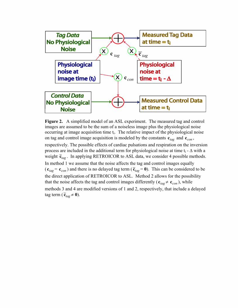
Figure 2. A simplified model of an ASL experiment. The measured tag and control images are assumed to be the sum of a noiseless image plus the physiological noise occurring at image acquisition time ti. The relative impact of the physiological noise on tag and control image acquisition is modeled by the constants c and c , respectively. The possible effects of cardiac pulsations and respiration on the inversion process are included in the additional term for physiological noise at time t

tag con

i - ∆ with a weight tagc

con

. In applying RETROICOR to ASL data, we consider 4 possible methods. In method 1 we assume that the noise affects the tag and control images equally (c = c ) and there is no delayed tag term (tag tagc = 0). This can be considered to be the direct application of RETROICOR to ASL. Method 2 allows for the possibility that the noise affects the tag and control images differently ( ≠ c ), while methods 3 and 4 are modified versions of 1 and 2, respectively, that include a delayed tag term (

tagc con

tagc ≠ 0).

Figure 3. Example showing calculation of cardiac phase (b). Peak of the cardiac cycle is denoted by a green x in (a). Calculation of cardiac phase for image number 3 is explained as follows: The 3rd TTL pulse shown in (a) corresponds to image number 3. The difference between the time that image 3 is sampled and the time of the preceding cardiac peak is approximately 0.3 sec. The difference in time between this cardiac peak and the following cardiac peak is approximately 1.2 sec. Referring to equation 11, cardiac phase at image 3 equates to

4.12.13.02]3[ == πϕc

Figure 4. Example showing calculation of respiratory phase (c). Peak respiratory activity shown in (a) is roughly 80 % of maximum respiration during the collected time series. Respiratory amplitude histogram is shown in (b). Bin values in (b) span

thru with intervals of 0 . Calculation of respiratory phase for image number 3 is explained as follows: The 3

max01.0 R maxR max01. Rrd TTL pulse shown in (a) corresponds

to image number 3. The respiratory activity during image 3 is 50% of maximum respiration during the imaging experiment. The number of occurrences in bin values from 0.01 to 0.50 is 6704. The sum of all occurrences is 11204. is positive. Referring to equation 12, respiratory phase at image number 3 is

)/sgn( dtdR

9112046704 .1=]3[ = πϕr

Figure 5. Example data from one voxel showing estimated (a) cardiac and (b) respiratory components estimated using BOLD physiological correction described in section 2.3.1. In addition, measured (a) cardiac and (b) respiratory signals that are down-sampled to 4 Hz are shown.

Figure 6. Data for BOLD images acquired at a TR of 250 ms. Image intensity corresponds to the sum of the Fourier spectrum over a frequency band that encompasses the respiratory peak frequency ( 0 Hz05.03. ± ). Column 1 shows the uncorrected data, column 2 shows the corrected data, and column 3 shows the difference between the two. Each row corresponds to data from one slice (slices 1 to 3). All images are scaled equally.

Figure 7. Data for BOLD images acquired at a TR of 250 ms. Image intensity corresponds to the sum of the Fourier spectrum over a frequency band that encompasses the cardiac peak frequency ( 0 Hz05.09. ± ). Column 1 shows the uncorrected data, column 2 shows the corrected data, and column 3 shows the difference between the two. Each row corresponds to data from one slice (slices 1 to 3). All images are scaled equally.

Figure 8. Fourier spectra of a single voxel (BOLD, TR = 250ms). (a) Spectra before and after noise correction. (b) Spectra of the physiological data resampled to the image sample frequency. (c) Spectra of the physiological data at the original sampling frequency of 40 Hz.

Figure 9. Example of resting-state (BOLD, TR = 250 ms) time series (a) before and (b) after correction. The standard deviation of each time series is also shown.

Figure 10. Data for BOLD images resampled to a TR of 2000 ms. Image intensity corresponds to the sum of the Fourier spectrum over a frequency band that encompasses the respiratory peak frequency and aliased cardiac peak frequency ( 0 ). Column 1 shows the uncorrected data, column 2 shows the corrected data, and column 3 shows the difference between the two. Each row corresponds to data from one slice (slices 1 to 3). All images are scaled equally.

Hz05.03. ±

Figure 11. Fourier spectra of a single voxel (BOLD, TR = 2000ms). (a) Spectra before and after noise correction. (b) Spectra of the physiological data resampled to the image sample frequency. (c) Spectra of the physiological data at the original sampling frequency of 40 Hz.

Figure 12. Example of resting-state (BOLD, TR = 2000 ms) time series (a) before and (b) after correction. The standard deviation of each time series is also shown.

Figure 13. F statistic versus delay time. The average F statistic of all voxels that exceed the threshold F statistic corresponding to a p value of 0.05 is shown. Plots are normalized to maximum F statistic of each slice. Average F statistic peaks at delay times of 850 ms, 900 ms and 950 ms for slices 1, 2, and 3, respectively. Data shown here are for subject 1.

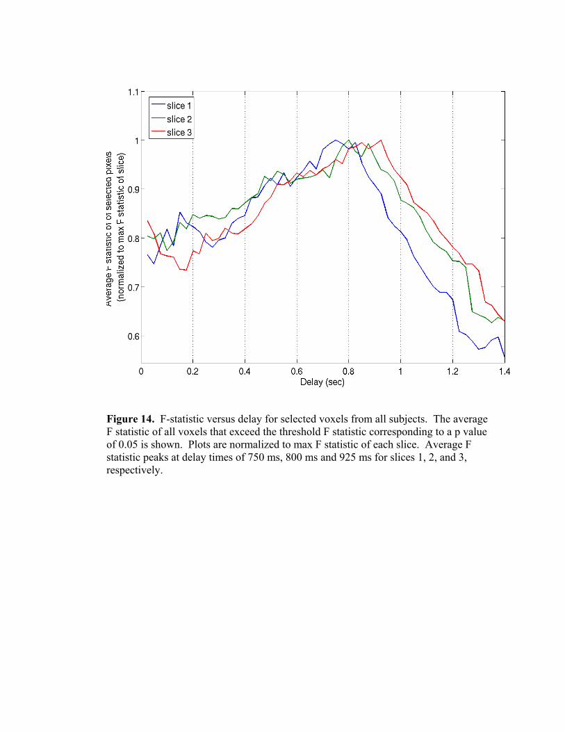
Figure 14. F-statistic versus delay for selected voxels from all subjects. The average F statistic of all voxels that exceed the threshold F statistic corresponding to a p value of 0.05 is shown. Plots are normalized to max F statistic of each slice. Average F statistic peaks at delay times of 750 ms, 800 ms and 925 ms for slices 1, 2, and 3, respectively.

Figure 15. Average number of voxels for subject 1 that exhibit an F statistic above a specified threshold. p-values corresponding to thresholds range from 0.0 to 0.05.

Figure 16. Average number of voxels across all subjects that exhibit an F statistic above a specified threshold. p-values corresponding to thresholds range from 0.0 to 0.05.

Figure 17. Example of a perfusion time series (a) before and (b) after correction (method 4) for subject 1. Green dotted line denotes time during which the stimulus was shown to the subject.

Figure 18. Example of a correlation map overlaid on an average perfusion map for subject 1. Results are shown before and after correction (method 4). Average cc and number of voxels above a threshold of 0.4 are summarized below each map.

Average # of voxels above cc=0.4

0.000 20.000 40.000 60.000 80.000

100.000 120.000 140.000 160.000

No Correction

Method 1 Method 3 Method 2 Method 4

Figure 19. Average number of voxels that exceed a correlation threshold of 0.4 across all subjects. Results are shown for no correction and correction with methods 1 – 4.

REFERENCES Buxton, R. B. (2002). Introduction to Functional Magnetic Resonance Imaging.

Cambridge, Press Syndicate for the University of Cambridge. Cox, R. W. (1996). "AFNI: software for analysis and visualization of functional

magnetic resonance neuroimages." Comput Biomed Res 29(3): 162-73. Dagli, M. S., J. E. Ingeholm, et al. (1999). "Localization of cardiac-induced signal

change in fMRI." Neuroimage 9(4): 407-15. Detre, J. A., J. S. Leigh, et al. (1992). "Perfusion imaging." Magn Reson Med 23(1):

37-45. Frank, L. R., R. B. Buxton, et al. (2001). "Estimation of respiration-induced noise

fluctuations from undersampled multislice fMRI data." Magn Reson Med 45(4): 635-44.

Glover, G. H., T. Q. Li, et al. (2000). "Image-based method for retrospective correction of physiological motion effects in fMRI: RETROICOR." Magn Reson Med 44(1): 162-7.

Hu, X., T. H. Le, et al. (1995). "Retrospective estimation and correction of physiological fluctuation in functional MRI." Magn Reson Med 34(2): 201-12.

Liu, T. T., L. R. Frank, et al. (2001). "Detection power, estimation efficiency, and predictability in event-related fMRI." Neuroimage 13(4): 759-73.

Liu, T. T., E. C. Wong, et al. (2002). "Analysis and design of perfusion-based event-related fMRI experiments." Neuroimage 16(1): 269-82.

Luh, W. M., E. C. Wong, et al. (2000). "Comparison of simultaneously measured perfusion and BOLD signal increases during brain activation with T(1)-based tissue identification." Magn Reson Med 44(1): 137-43.

Noll, D. C. and W. Schneider (1994). "Theory, simulation, and compensation of physiological motion artifacts in functional MRI." IEEE International Conference on Imaging Processing, Austin, Texas: 40.

Pfeuffer, J., G. Adriany, et al. (2002). "Perfusion-based high-resolution functional imaging in the human brain at 7 Tesla." Magn Reson Med 47(5): 903-11.

Pfeuffer, J., P. F. Van de Moortele, et al. (2002). "Correction of physiologically induced global off-resonance effects in dynamic echo-planar and spiral functional imaging." Magn Reson Med 47(2): 344-53.

Restom, K., Y. Behzadi, et al. (2004). Image based physiological noise correction for perfusion-based fMRI. Twelfth Meeting, International Society for Magnetic Resonance in Medicine, Kyoto, Japan.

Turner, R., P. Jezzard, et al. (1993). "Functional mapping of the human visual cortex at 4 and 1.5 tesla using deoxygenation contrast EPI." Magn Reson Med 29(2): 277-9.

Wong, E. C., R. B. Buxton, et al. (1997). "Implementation of quantitative perfusion imaging techniques for functional brain mapping using pulsed arterial spin labeling." NMR Biomed 10(4-5): 237-49.

Wong, E. C., R. B. Buxton, et al. (1998). "Quantitative imaging of perfusion using a single subtraction (QUIPSS and QUIPSS II)." Magn Reson Med 39(5): 702-8.