ECOGRAPHY 25: 578–600, 2002

Illustrations and guidelines for selecting statistical methods forquantifying spatial pattern in ecological data

J. N. Perry, A. M. Liebhold, M. S. Rosenberg, J. Dungan, M. Miriti, A. Jakomulska and S. Citron-Pousty

Perry, J. N., Liebhold, A. M., Rosenberg, M. S., Dungan, J., Miriti, M., Jakomulska,A. and Citron-Pousty, S. 2002. Illustrations and guidelines for selecting statisticalmethods for quantifying spatial pattern in ecological data. – Ecography 25: 578–600.

This paper aims to provide guidance to ecologists with limited experience in spatialanalysis to help in their choice of techniques. It uses examples to compare methodsof spatial analysis for ecological field data. A taxonomy of different data types ispresented, including point- and area-referenced data, with and without attributes.Spatially and non-spatially explicit data are distinguished. The effects of samplingand other transformations that convert one data type to another are discussed; thepossible loss of spatial information is considered.Techniques for analyzing spatial pattern, developed in plant ecology, animal ecology,landscape ecology, geostatistics and applied statistics are reviewed briefly and theiroverlap in methodology and philosophy noted. The techniques are categorizedaccording to their output and the inferences that may be drawn from them, in adiscursive style without formulae. Methods are compared for four case studies withfield data covering a range of types. These are: 1) percentage cover of three shrubsalong a line transect; 2) locations and volume of a desert plant in a 1 ha area; 3) aremotely-sensed spectral index and elevation from 105 km2 of a mountainous region;and 4) land cover from three rangeland types within 800 km2 of a coastal region.Initial approaches utilize mapping, frequency distributions and variance-mean in-dices. Analysis techniques we compare include: local quadrat variance, block quadratvariance, correlograms, variograms, angular correlation, directional variograms,wavelets, SADIE, nearest neighbour methods, Ripley’s L� (t), and various landscapeecology metrics.Our advice to ecologists is to use simple visualization techniques for initial analysis,and subsequently to select methods that are appropriate for the data type and thatanswer their specific questions of interest. It is usually prudent to employ severaldifferent techniques.

J. N. Perry ( joe.perry@bbsrc.ac.uk), PIE Di�ision, Rothamsted Experimental Station,Harpenden, Hertfordshire, U.K. AL5 2JQ. – A. M. Leibhold, Northeastern ResearchStation, USDA Forest Ser�ice, Morgantown, WV 26505, USA. – M. S. Rosenberg,Dept of Biology, Arizona State Uni�., Tempe, AZ 85287-1501, USA. – J. Dungan,NASA Ames Research Center, Moffett Field, CA 94035-1000, USA. – M. Miriti,Dept of Ecology and E�olution, State Uni�. of New York, Stony Brook, NY 11794-5245, USA. – A. Jakomulska, Remote Sensing of En�ironment Laboratory, Faculty ofGeography and Regional Studies, Uni�. of Warsaw, Warsaw PL-00-92, Poland. – S.Citron-Pousty, Dept of Ecology and E�olutionary Biology, Uni�. of Connecticut,Storrs, CT 06269, USA.

Current consensus within ecology that ‘‘space is thefinal frontier’’ (Liebhold et al. 1993) is expressed byintense interest in issues of spatial scale (Wiens 1989,Dungan et al. 2002), metapopulation dynamics (Hanski

and Gilpin 1997), spatio-temporal dynamics (Hassell etal. 1991), spatially-explicit modelling (Silvertown et al.1992) and spatial synchrony (Bjørnstad et al. 1999).Temporal ecological processes have been well studied

Accepted 14 January 2002

Copyright © ECOGRAPHY 2002ISSN 0906-7590

ECOGRAPHY 25:5 (2002)578

since the work of Lotka and Volterra (May 1976)was applied to insect population dynamics some sixtyyears ago. By contrast, progress in spatial analysiswas somewhat hampered by the lack of computingresources required, and intensive work began perhapstwo or three decades later.

When ecologists seek spatial pattern, evidence ofspatial non-randomness, they find it is the rule ratherthan the exception. The natural world is indeed apatchy place (Dale 1999), as we might expect, becauserandomness implies the absence of behaviour, and sois unlikely a priori on evolutionary grounds (Tayloret al. 1978). Ecologists study spatial pattern to inferthe existence of underlying processes, such as move-ment or responses to environmental heterogeneity.Spatial structure may indicate intraspecific and inter-specific interactions such as competition, predation,and reproduction. Observed heterogeneity may alsobe driven by resource availability. Care is required ininferring causation, since many different processesmay generate the same spatial pattern. Spatial patternhas implications for both the theoretical issues out-lined above and applied problems such as the man-agement of threatened species. Knowledge of spatialstructure can assist in the adjustment of statisticaltests and the improvement of sampling design (Legen-dre et al. 2002).

Although spatial analysis reveals spatial pattern, itis usually an empirical approach based on observa-tional data, and is rarely model-based. As such, it isthe forerunner and facilitator of the formation of spe-cific testable hypotheses that may later be tackled ex-perimentally, in manipulative studies. Only then canthis process generate new ecological theory. The levelat which data are analyzed depends critically on theamount of detail in the information already gathered,concerning the biology and ecology of the speciesstudied. Models can only be formed when there isconsiderable detailed information about life-stages,their dynamics, demography, movement, behaviour,etc. The approach outlined here is more generic andless specific; it is targeted at situations when data arecollected from initial studies, relatively early in a pro-ject. When more is known, models of spatial pattern(Keitt et al. 2002) may be used to support inferenceor for estimation and prediction in unsampled loca-tions.

Methods for analyzing spatial pattern have beendeveloped in a wide variety of disciplines. Seminalpapers include Bliss (1941) in animal ecology, Watt(1947) in plant communities, Skellam (1952) in statis-tics, Matern (1986) in forestry and Rossi et al. (1992)in geostatistics. This wide variety has led to someoverlap of methodology and philosophy (Getis 1991,Dale et al. 2002). As ecologists approach a spatialproblem for the first time, they are often over-whelmed by the multiplicity of available techniques,uncertain about which set of methods to use, per-

plexed by the consequences of their choice of meth-ods, and mystified as to the interpretation ofseemingly conflicting results.

The purpose of this paper is to provide a frame-work for taking such decisions concerning analyticalapproaches and interpretations. This we do by com-paring and contrasting many commonly-used tech-niques, using four case-studies with field data. Westart by describing the types of spatial data that maybe encountered. We then briefly describe a variety oftechniques that can be used to analyze data of eachform, and attempt a simple characterization in termsof their output. All of the methods we will illustratehave been described elsewhere in detail. We next usethe four real data sets to illustrate the results that areobtained from each analysis, focusing on how themethods differ with regard to appropriateness fordata type and information provided. There have beenfew previous studies that have compared and con-trasted different techniques, other than the paper ofLegendre and Fortin (1989), text books, and informalsurveys such as that reported at: �http://www.stat.wisc.edu/statistics/survey/survey.html�. Thispaper differs from those due to the greater scope ofboth the types of data and statistical procedures illus-trated.

Types of spatial data

We summarize spatial data types according to thestandard geographic system that defines points, lines,areas and volumes (Burrough and McDonnell 1998),but we restrict discussion to the more ubiquitouspoint- and area-referenced data. There is a naturalhierarchy of information contained within data types;some may be derived from others higher in this hier-archy, through transformation or sampling.

Dimensionality of study arena

Ecological data are often collected along a one-di-mensional linear transect (Fig. 1a, below), defined bythe set of coordinates {L} that comprise it (bold typedenotes a set of values represented by a vector). Thearena more usually studied is two-dimensional, oftenrectangular, although irregular shapes (e.g. Fig. 1a,top) are common. Definition of the boundary of atwo-dimensional arena requires considerably morecomplexity than for a transect; the descriptor set {A}must comprise at least three pairs of (x, y) coordi-nates. Rarely, the area studied may explicitly excludesome regions within its boundary (e.g. Korie et al.2000), perhaps because some habitat within the areacannot be utilized by the species studied.

ECOGRAPHY 25:5 (2002) 579

Subdivision of the study arena

The study arena may be subdivided spatially with nointrinsic loss of information into contiguous regions(e.g. Fig. 1b) such as physiographic provinces (Baileyand Ropes 1998), or defined by some qualitative factor,such as habitat type, or quantitative variable, such astree density in four classes.

If it is not possible to record data as a completecensus of the study arena, then samples may be takenover smaller proportions of it. For example, an areamay be sampled by several quadrats. When subareasare defined, then the quadrats are usually placed so asto represent them. Alternatively, the quadrats may beplaced at random, or in some pre-determined arrange-ment, often to form a rectangular grid (Fig. 1c). Occa-sionally, samples are taken at points. Sampling resultsin a loss of information compared to a complete census,and caution should be taken to ensure that the effectsof this are minimized (see Dungan et al. 2002). Statisti-cal methods must be used to relate the sample to thelarger population and to make inferences.

A sampling plan may be characterized by a combina-tion of variables termed the extent, sample unit size(known in geostatistics as the ‘‘support’’) and lag. Theextent describes the dimensions of the study arena, andits area, A. The sample unit size is the area of thequadrat (dw in the example in Fig. 1c). The lag refers to

the distance between each quadrat in a grid (ld and lw,in the x and y directions, respectively, in Fig. 1c). Forcontiguous subareas with no sampling, the lag is zero.Changes to extent, support and lag may influence theinferences drawn from analysis (Dungan et al. 2002).

Data types

We distinguish three prevalent spatial data types,defined by the topology of the entity to which therecorded information refers. These are 1) point-refer-enced (Fig. 1d), 2) area-referenced (Fig. 2), and 3)non-spatially referenced (attribute-only).

Point-referenced data are common in plant ecology;forms derived from it are widespread in terrestrialecology. The simplest point-referenced data are a com-plete census of the individuals recorded along a transect(Fig. 1d, below). Each individual is considered identicalto all others and the only information recorded is itslocation. This type is denoted as (x). An example wouldbe the locations of a particular weed species along afield margin. For a two-dimensional arena, the point-referenced data denoted as (x, y) describes the cen-sussed locations of all individuals within it, withreference to two coordinate dimensions (e.g. Fig. 1d,top).

Fig. 1. (a, below) Example ofone-dimensional transect withlocation described by the setL, comprising twox-coordinates; (a, top)example of two-dimensionalstudy arena, with locationdescribed by the set of (x, y)boundary coordinates A, andwith area denoted by A. (b)The entire study arena isdivided into six contiguoussubareas of unequal size andshape. (c) Six parts of thestudy arena are sampled witha rectangular grid ofnon-contiguous quadrats,each one representative ofthat subarea, shown in (b), inwhich it is located. Eachquadrat is itself rectangular,with dimensions d and w, andseparated from its neighbourby distances ld and lw, in thex and y directions,respectively. (d) Example ofpoint-referenced data in theform of censussed, mappedindividuals in the study arena(top) and transect (below) of(a).

580 ECOGRAPHY 25:5 (2002)

Fig. 2. Example of area-referenced geographic data, used typ-ically in landscape ecology. The study arena of Fig. 1a hasbeen partitioned into areas, each with one of three attributes,denoted by the shading. Areas may be polygonal or irregularlyshaped with curved boundaries. Also represented are a linearfeature, denoted RS, and a point, denoted T.

let, Thiessen or Voronoi (see Dale 1999: Fig. 1.4 for anexample). A closely related technique is the Delaunaytriangulation. These techniques leave the (x, y) coordi-nates of the data unchanged. They effectively createadditional, derived, area-referenced data, similar to thatdescribed in section 2) below.

Point-referenced (x, y) data may be amalgamatedinto a single value, to represent a subarea. This resultsin partial loss of spatial information, since the originallocations can no longer be recovered. The resultingderived data are still explicitly spatial and retain theform (x�, y�), but x� and y� must now be defined, forexample as the centroids of the subareas, used to trans-form the (x, y) data of Fig. 1d to the (x�, y�, z�) datatype in Fig. 3c. In this example, a value of z� for eachsubarea has been derived from the count of the numberof individuals within it. Comparing the two figuresshows that almost all the information concerning clus-tering has been removed from the derived data. Fortransformations of (x, y, z) data, amalgamation of thez variable may also be achieved in very many ways,such as the mean magnitude of the z attribute, wherethe averaging is over the individuals located within eachsubarea.

Sampled data from quadrats is always derived, bydefinition, since all the data recorded from within thequadrat are somehow aggregated, to yield a singlerepresentative value. Usually, the derived (x�, y�) com-ponent representing the location of each quadrat isdefined as its centroid, as in Fig. 3d, where the z’ valuefor each of the quadrats in Fig. 1c has been derivedfrom the count of the number of individuals containedwithin it. Observe how much variability is induced into

For any spatial data type, further information maybe available for each individual, through the recordingof an extra attribute(s), z; such data are denoted (x, z)or (x, y, z). Attributes may have different forms, ofwhich the simplest is a categorical quantal variable(male or female, dead or alive, Fig. 3a). Another formof z attribute might be an ordered categorical qualita-tive variable, such as a life-stage. Alternatively, it couldbe a quantitative variable, such as the magnitude of aninnoculum (Fig. 3b).

Many forms of data may be derived. One transfor-mation frequently applied to two-dimensional point-ref-erenced ecological data divides up the study arenaaccording to the locations of individuals, into a mean-ingful tessellation of polygons, often named for Dirich-

Fig. 3. Further examples offorms of point-referenceddata. The censussed mappedindividuals of Fig. 1d, (a)with additional quantalattribute; (b) with additionalcontinuous attribute withmagnitude indicated by sizeof symbol; (c) as countswithin each of the sixcontiguous dashed subareasof Fig. 1b; (d) as countssampled by the six dashednon-contiguous quadrats ofFig. 1c.

ECOGRAPHY 25:5 (2002) 581

the counts of Fig. 3d by the sampling process, com-pared with the censussed values shown in Fig. 3c;whatever loss of information is involved in derivedcensussed data, the loss from sampled data will begreater. Also, note the difference between recording a zattribute(s) on exhaustively censussed point-referencedindividuals, and taking a point sample of an attributethat is a continuously distributed variable over thestudy arena, such as elevation. Both may involve irreg-ularly-spaced data of the form (x, y, z), but the latterhas the properties of a sample, with the concomitantfeatures of uncertainty and the intention to representsome larger unknown population.

Area-referenced data are common in landscape ecol-ogy and geography. All of the variations of point-refer-enced data discussed above apply equally to thearea-referenced data exemplified in Fig. 2. This type iscommonly represented either by a vector form, (A, z),where location coordinates defining each (possibly ir-regular) area are associated with attribute(s), or by araster form, where locations are addressed by a grid ofCartesian coordinates and attributes pertain to a cell offixed area at that location. Note that raster data can bestored as point-referenced data (x, y, z) but mustinclude the crucial information of grid cell size; thisrepresentation is substantially equivalent to point-refer-enced data in subareas, where the loss of information issmall and offset by a very large number of subareas.

In geography, a dichotomy is recognized betweenso-called ‘‘object’’ and ‘‘field’’ data models (Peuquet1984, Gustafson 1998, Peuquet et al. 1999). The objectmodel considers two-dimensional arenas populated bydiscrete entities whereas underlying the field model arevariables assumed to vary continuously on a surface.Area-referenced data can be considered as either; withinGeographic Information Systems software (Burroughand McDonnell 1998) (A, z) data are often representedas polygonal.

Sometimes, explicit spatial information might notexist, or if the data for analysis is recycled from previ-ous results, the information may have been degradedand lack the detail of the original records. Some meth-ods of data recording or amalgamation remove allexplicit spatial information. For example, a commonand powerful entity in spatial pattern analysis is termeda nearest neighbour (NN) distance (Donnelly 1978,Diggle 1983, Ripley 1988), defined for each censussedindividual as the distance to its nearest neighbour.Hence, in the (x, y) data shown in Fig. 1d above, theindividual labelled P has the individual labelled Q as itsnearest neighbour and the distance PQ would be theNN distance associated with P. As can be seen, therelationship is not necessarily commutative, since thenearest neighbour of Q is not P. The set of NNdistances for all individuals is not spatially-referenced,so is denoted by (z). However, it contains much implicitinformation concerning location, and may be used to

test for spatial randomness. A further example is thefrequency distribution of counts in subareas or samples(e.g. the set z={3, 4, 6, 7, 7, 9} from Fig. 3c), strippedof its (x, y) coordinate information. From these sixcounts may be derived associated statistics such as thesample mean, sample variance, and quantities such asthe variance to mean ratio, known as the index ofdispersion (Fisher et al. 1922), I, which in this case isexactly 4. Note how I fails to capture any of the patternin the original Fig. 1d.

Data taxonomy

Other proposals for data taxonomy have been made;some are not helpful because they are specific to disci-plines tangential to mainstream ecology (e.g. Gustafson1998). Cressie’s (1991) taxonomy is not recommendedbecause it makes insufficient distinction between theinformation available and the collection methods usedto record it, particularly to reflect the effect of sam-pling. Also, it formally defines lattice data as encom-passing a finite, countable set of spatial locations, whileconfusingly exemplifying it by reference to remote sens-ing and medical image data that are both spatiallycontinuous in nature. Additionally, it would benefitfrom a revision to link the term ‘‘geostatistical’’ withmodels or methods for spatial analysis, rather than withtypes of data.

Techniques for spatial analysis

Characteristics of spatial pattern

Many terms are used in ecology to describe variousaspects of generic non-randomness in spatial data. Theterms ‘‘aggregated’’, ‘‘patchy’’, ‘‘contagious’’, ‘‘clus-tered’’ and ‘‘clumped’’ all refer to positive, or ‘‘attrac-tive’’, associations between individuals in point-referenced data, such as those in Fig. 4a. The terms‘‘autocorrelated’’, ‘‘structured’’ and ‘‘spatial depen-dence’’ indicate the tendency of nearby samples to haveattribute values more similar than those farther apart.Conversely, the terms ‘‘negatively autocorrelated’’, ‘‘in-hibited’’, ‘‘uniform’’, ‘‘regular’’ and ‘‘even’’ refer tonegative or repulsive interactions between individuals,such as those in Fig. 4b. The term ‘‘overdispersion’’ hasbeen used very confusingly in the past, to indicateexcess variability or heterogeneity by statisticians andregularity of distribution by ecologists; for this reasonwe agree with Southwood’s (1966, p. 25) recommenda-tion that this and its antonym ‘‘underdispersion’’ beused sparingly, and then only with rigorous definitions.

The large number of methods derived for spatialanalysis reflect the multitude of non-random character-istics that may be of interest to ecologists and the

582 ECOGRAPHY 25:5 (2002)

Fig. 4. Point locations of 32individuals: (a) aggregatedinto 8 clusters, each with arandom number ofindividuals, and centred onrandom locations; (b)arranged regularly; (c) thatdisplay spatial anisotropy; (d)that display non-stationaryspatial structure, with half ofthe individuals aggregatedinto four clusters towards thetop and left of the studyarena and the other half, inthe bottom-right of the area,arranged randomly. Note thatin d the intensity of theprocess is roughly equal inthe two parts of the area. Inboth a and b, one of thepoints has been labelled Aand two circles, radii t1 andt2, are shown centred on A.

corresponding multiplicity of mechanisms that generatethem. Most methods identify particular characteristicsof pattern, ranging from generic statistical measures,such as coefficient of variation among samples, to morespecialized methods that address explicit ecologicalquestions, such as indices of landscape habitat patchshape. Occasionally, methods such as geostatistics havearisen in one discipline and proved so useful that theyhave been embraced by mainstream ecology (Rossi etal. 1992, Liebhold et al. 1993). We focus on twelvemethods, exemplified in analyses of the case studies.Some methods, such as fractal analysis (Stoyan andStoyan 1994) or spectral methods (Mugglestone andRenshaw 1996), are omitted due to constraints of space.Detailed descriptions of methods may be found in citedsources or in the companion paper of Dale et al. (2002).

Most methods seek to compare some feature of thespatial process ‘‘here’’ (at some local reference point),with the same feature ‘‘elsewhere’’, i.e. in another loca-tion(s). The reference point could be a randomly chosenlocation or individual. The feature described might be acount of a defined set of other individuals; or an

attribute, for example the volume of some organism; ora derived value, such as local density. The other loca-tion(s) may be a particular distance away in some givendirection; or defined by a given interval centred on thereference point; or the next contiguous area in a se-quence; or the nth nearest individual. The definition‘‘local’’ may shift, systematically or randomly, to en-compass different parts of the study arena, in turn.

Methods vary in the degree of information theyimpart. The simplest methods are descriptive displaysof spatial information, consistent with Chatfield’s(1985) principles of initial data analysis. We stress theutility of mapping and simple summary statistics as afirst step in the analysis of spatial data (Korie et al.1998), and advocate the work of Tufte (1997) and Carr(1999) as an innovative source of ideas for visual pre-sentation. More sophisticated methods allow inferencein the form of a test of the null hypothesis, sometimesmore complex than that of complete spatial random-ness. Yet further information is offered by methodsthat estimate quantities. Finally, there are methods thatfit spatial models, if enough data are available (Keitt etal. 2002).

ECOGRAPHY 25:5 (2002) 583

Many ecological data sets exhibit different spatialpattern when viewed at one spatial extent than atanother, a ‘‘scale’’ effect. For example, the point loca-tions in Fig. 4a are aggregated into clusters at smallspatial extents, although the clusters themselves have arandom number of individuals and random locations.Certain methods are designed specifically to study therelationship between the degree of pattern and its scale(Table 1), and see Dungan et al. (2002).

Another common spatial characteristic of ecologicaldata is anisotropy, where the pattern itself changes withdirection. In Fig. 4c the clusters are elongate in aspecific direction and tend to be associated with eachother more strongly in that direction. Compare Fig. 4a,where the pattern is random with respect to direction.

Whereas global methods summarize patterns over thefull extent of the area studied, in recent years there hasbeen interest to develop methods that identify localvariation (Anselin 1995, Getis and Ord 1995, Ord andGetis 1995, Sokal et al. 1998a, b) in spatial characteris-tics, such as aggregation, within the sampling domain(Table 1). Local methods such as wavelets and SADIEcan be used to map and detect locations within thestudy arena that may drive the overall pattern, or whichare outliers. When the underlying process that generatespattern varies across different regions within the areastudied, a stationary model will not be appropriate. InFig. 4d, although the intensity of the point process isroughly equal in the two parts of the area, individualsare aggregated in one part and randomly distributed inanother. Many methods are based, to a small or largedegree, on stationarity assumptions.

Methods appropriate for different data types

Point-referenced data, (x, y)Questions asked of such data normally concern thespatial pattern of the individuals: are they clustered (asin Figs 1d, top and 4a) or regularly spaced (as in Figs1d, below and 4b), or do they occur at random loca-tions? Ripley (1977, 1988) derived a method based onthe indices, K� (t) and L� (t), scaled for intensity, thataverages the number of individuals within a distance tof a randomly chosen individual. For an individual inan aggregated pattern, for example point A in Fig. 4a,the expected number of individuals within a circle ofradius t1 that approximates to the dimensions of atypical cluster will be relatively large compared to thesame number of individuals distributed randomlywithin the study arena. As the radius of the circle isgradually increased, say to t2, the area encompassedextends outside the cluster to which A belongs, but notyet into other clusters, so there are few extra individualscounted. This characteristic increase in the count overparticular small intervals of t provides a signature tographs of L� (t) vs t, that may be formally tested by

comparison with corresponding graphs generated byMonte Carlo simulation (Diggle 1983) for random pat-terns. Note that for a regular pattern, as in Fig. 4b, thereverse is the case: the count is fewer than expected fort1 and greater for t2. Methods for this data type mustallow for edge effects (Ripley 1988, Haase 1995).

Point-referenced data with attributes, (x, y, z)Typical questions for such data are: is the apparentsegregation in Fig. 3a of the solid from the opensymbols real, and vice versa? Is the infection measuredby the quantitative degree of innoculum shown in Fig.3b dispersing from a point source, and if so, can weconfirm that the source is located close to the centre ofthe study arena? With such a continuous attribute it isoften of interest to determine whether its values aremore similar than expected to those nearby, or moreformally whether there exists detectable spatial autocor-relation, and if so, what is its relationship with thedistance between points? When there are several zattributes, we are usually interested to know whetherthe variables are positively spatially associated (Perry1998b, Liebhold and Sharov 1998) with each other ornegatively spatially associated (termed ‘‘dissociated’’),once any induced (dis)similarity due to their individualspatial structure is allowed for (Clifford et al. 1989,Bocard et al. 1992, Dutilleul 1993). Alternatively, dothey occur randomly with respect to one another?

Some methods that involve z-attributes are restrictedto regularly spaced (x) or (x, y) data on a grid (Table1). For example, ‘‘quadrat variance methods’’ (Dale1999) which include ‘‘two-term local quadrat variance’’(TTLQV) as well as 3TLQV and others, are usedpredominantly for one-dimensional regularly-spacedtransect data. Second-order comparisons are made be-tween blocks of a given length, say d, of contiguousquadrats, through computation of their variance. Ag-glomeration into blocks using increasing values of d,within a hierarchy, allows plots of variance against d.Since the blocks are contiguous, block size is identicalto the distance between block centres. The idea is thata peak in variance on this graph will indicate maximumcontrast between patch and gap, if there is a stationaryprocess with constant cluster size, at a distance equiva-lent to approximate cluster size. This allows the detec-tion, and in some cases the testing for significance ofspatial pattern along the transect. Their analogues intwo-dimensions include the block quadrat variancemethods for (x�, y�, z�) data where z� is a count, derivedfor insects by Bliss (1941), rediscovered for plants byGreig-Smith (1952) and later modifications such as4TLQV (Dale 1999).

Very closely related to these is a large class ofmethods that focus on the dependence of autocorrela-tion on distance. Here, blocks of quadrats are replacedby single units or individual locations. The averagevariance between a pair of units is calculated for a

584 ECOGRAPHY 25:5 (2002)

EC

OG

RA

PH

Y25:5

(2002)585

Table 1. Description of methods for analysis of spatial data.

AllowsType of data Original use Info. available Info. availableModel 1- or 2- Irregularly-Method Info. availabledimensions?on anisotropy? spaced unitshypothesis on localbased? at multiple

pattern? allowed?scales?tests?

possible no both yesyesyesRipley’s K and L, etc. noplant ecologypoint-referencedlocations, (x, y)

Quadrat variance methods yes no no 1 nopoint-referenced plant ecology no rarelylocations, (x, z)(TTLQV, etc.)

no rarely yes possible no 2 noplant ecologypoint-referencedBlock quadrat variancelocations withmethods (Greig-Smith,attributes, (x, y, z)4TLQV, etc.)point-referenced no yes yes yes no both yesCorrelograms (Moran’s I, geography

Geary’s c, etc.) locations withattributes, (x, y, z)

yes no both yesGeostatistics (variograms), (x, y, z) Earth sciences no no yesPQV

no both yesyes yesGeostatistics (kriging) yesyesEarth sciences(x, y, z)Angular correlation yes no 2 yes(x, y, z) geography no yes no

yes no yes both noWavelets (x, y, z) statistics no nono no yes both yesSADIE (x, y, z) insect ecology no yes

rarely no rarely no 2rarely yeslandscape ecologyarea-referencedLandscape ecology metricslocations with(edge density, shape

indices, etc.) attributes, (A, z)no yes no no no bothapplied yesVariance-mean methods non-spatially

entomologyreferenced data,(Morisita, Taylor, etc.)attributes only, (z)

yes no no no both yesplant ecology andNearest neighbour methods no(z)forestry

particular distance, d, and the relationship betweenvariance (or semi-variance) and d is graphed and stud-ied, thereby quantifying structure at multiple spatialextents. Some of these methods, Moran’s I (Moran1950) and Geary’s c, allow significance tests of com-plete spatial randomness (Cliff and Ord 1973, 1981,Sokal and Oden 1978, Oden 1984). Geostatistical meth-ods in this class include the variogram, correlogram,and covariance function. We include paired quadratvariance (PQV) in this section because, although strictlya quadrat variance method, the size of its block nevervaries; indeed, despite their independent development,the variogram and PQV are mathematically identicaland thus provide the same information (ver Hoef et al.1993, Dale and Mah 1998, Dale et al. 2002). Geostatis-tical methods are not generally used for hypothesistesting, but their associated models of spatial depen-dence are used for spatial interpolation, modelling andsimulation (Isaaks and Srivastava 1989, Rossi et al.1992). The idea underlying all the methods is thatspatial autocorrelation declines, and therefore varianceincreases, with increasing d, until some maximum vari-ance, termed the ‘‘sill’’, is reached, at a value of dtermed the ‘‘range’’. The range is an estimate of averagepatch and gap size. For very small d the variance,termed the ‘‘nugget’’, although a minimum, may still benon-zero; it is equated to measurement error plus thevariance at smaller unit sizes. When z is a dummy (0, 1)variable, measuring presence, some methods in thissection (such as indicator variograms) are effectivelyutilizing (x, y) data.

Many methods have been adapted for the study ofanisotropy (Oden and Sokal 1986, Isaaks and Srivas-tava 1989, Falsetti and Sokal 1993) and local informa-tion (Anselin 1995, Getis and Ord 1995, Ord and Getis1995, Sokal et al. 1998a, b). Specific methods (Table 1)to detect anisotropy include Rosenberg (2000) and anangular method using spatial correlation, derived bySimon (1997). The latter projects each (x, y, z) pointonto an axis in a test direction, say �, then calculatesthe correlation, r, between the positions of the projectedpoints along this �-axis and the z-attribute. The valuesof (�, r) are then plotted in polar coordinates; a bulge inthe resulting curve indicates the direction of greatestchange in z.

Wavelet analysis may also be used to quantify spatialpattern over a variety of spatial extents, usually forone-dimensional data. It has much in common with themethods described above, albeit based on a differentstatistical approach (Bradshaw and Spies 1992, Daleand Mah 1998). The emphasis is on the ‘‘decomposi-tion’’ of the data into repeating patterns that are com-pared with the wavelet function’s shape over varyingwindow-widths, which are equivalent to distance lags.In this there are similarities to the quadrat variancemethods (Dale et al. 2002), but wavelets allow contrastsof a specific and more complex functional form, using

shapes such as the ‘‘Mexican hat’’ (Dale 1999). Apowerful feature of this method is the lack of anystationarity assumption.

SADIE is a class of methods designed to detectspatial pattern in the form of clusters, either of patchesor gaps (Perry et al. 1999). The calculations (Dale et al.2002) also involve comparisons of local density withthose elsewhere, but made across the whole study arenasimultaneously. Each sample unit is ascribed an indexof clustering, and the overall degree of clustering intopatches and gaps is assessed by a randomization test. Aspecific extension to spatial association (Winder et al.2001) is made by comparing the clustering indices oftwo sets of data across the sample units. A local indexof association, �k, may be derived at each sample unit,k, and these may be combined to give an overall value,X. The power of these methods comes from the abilityto describe and map local variation of spatial patternand association.

Area-referenced data (A), (A, z)Data that are area-referenced are common in landscapeecology, particularly in polygonal form. The methodol-ogy for their analysis has not advanced as fast as othertechniques described here. Only few involve inferentialtests; they are largely descriptive. As for point data, oneoption is to sample by overlaying a grid and convert to(x, y, z) spatially-referenced attribute data (see aboveand Discussion). However, if the degree of fragmenta-tion is of particular interest then methods such as thosedescribed in Turner and Gardner (1991) and McGarigaland Marks (1995) may be applied to polygonal data ineither raster or vector form. Patch size and its coeffi-cient of variation (CV) are examples of the numerousindices; there is no space here for an exhaustive list.The latter is a measure of landscape fragmentation andheterogeneity but with important limitations (McGari-gal and Marks 1995). Edge density (Morgan and Gates1982), defined as a measure of edge length standardizedby enclosed area, is positively related to the degree offragmentation of the habitat, but also to its shape. Forregular shapes it is minimum for a circle, and maximalfor a linear feature. Total edge length is the sum of alllengths of edges of patches of one landscape type.Mean shape index, the ratio of perimeter to area, is ameasure of shape complexity; it approaches unity forperfect figures such as circles and increases with shapeirregularity (McGarigal and Marks 1995). When sam-pling relatively small areas, the area-weighted shapeindex is considered more meaningful, because it givesgreater weight to large polygons.

Attribute-only data (z)NN methods (Ripley 1977, 1988, Diggle 1983) are usedto analyze the distance from each of the individuals ina set of point-referenced data to its pth nearest neigh-

586 ECOGRAPHY 25:5 (2002)

bour, where p is usually unity. The set of distances isnot spatially explicit, even though it is derived frompoint-referenced locations. Hypothesis tests (Clark andEvans 1954) are usually based on the expected distribu-tion of such distances for a random arrangement ofindividuals. Highly clustered patterns tend to have rela-tively small (e.g. Fig. 4a), and regular patterns (e.g. Fig.4b) relatively large NN distances, respectively. They aresimilar to methods like Ripley’s L� (t) function in thatthey must be adjusted to allow for edge effects, butdiffer from them in that they utilize less spatial infor-mation and cannot identify pattern at multiple spatialextents.

Early studies of spatial pattern such as Bliss (1941)were based on summary statistics from frequency distri-butions (David and Moore 1954), and used little or nospatially-explicit data. Techniques relied on the factthat samples of randomly arranged individuals wouldyield counts that followed the Poisson distribution, butan observed Poisson distribution does not necessarilyimply randomness (Hurlbert 1990). Indeed, the set ofcounts: {0, 0, 1, 1, 2, 2, 2, 2, 3, 3, 5}, conforms closelyto a Poisson distribution, but if sampled in that orderalong a line transect shows an obvious linear trenddeparting strongly from randomness. Recent methods(Upton and Fingleton 1985, Perry and Woiwod 1992)include the index of dispersion I, Morista’s index,Lloyd’s (1967) index of mean crowding and Taylor’spower law (Taylor et al. 1978), used extensively inanimal ecology. Jumars et al. (1977) and Perry (1998a)have cautioned users to distinguish non-randomness inthe form of statistical variance-heterogeneity from truespatial non-randomness. The only valid spatial infer-ence possible to make from an observation of variance-heterogeneity is that there must be spatial pattern forsome unknown support smaller than that used to derivethe observed counts.

Origins of methods

While it can be shown that many of the methodsdescribed above are computationally similar (Dale et al.2002), it is worth noting that many differences amongthe methods can be attributed to their historical devel-opment in different disciplines (Table 1). In appliedentomology, limited computational resources before1970 precluded the widespread development of methodsthat utilized specific spatial coordinates, although theSADIE method now exists to address this issue. Later,methods developed for plant ecology were applied totwo-dimensional coordinate locations of individuals,but often lacked a tractable underlying statisticalmodel. Geostatistical methods were developed for prob-lems in the applied Earth sciences and emphasizedestimation rather than the detection of spatial patternby hypothesis testing. However, their development from

an underlying generic statistical model has made thesemethods useful for purposes of spatial interpolationand simulation, and they are applied increasingly toecological problems (Rossi et al. 1992, Liebhold et al.1993).

Case studies

Four case studies are used to illustrate the applicationof the methods outlined above to the data types dis-cussed above. These exemplify comparisons betweenmethods, regarding their applicability to answer partic-ular questions, their ability to provide different types ofinformation and to allow contrasting inferences.

Case study 1: counts of three shrub species alonga transect

The data (Dale and Zbigniewicz 1997) are censussedpercentage cover of each of six boreal shrub species, ofwhich only three are considered here. They are, in orderof abundance, Betula glandulosa, Salix glauca, andPicea glauca, measured between 1 and 3 m height.Cover was measured, along a linear transect of 1001contiguous quadrats, each 0.1 m2, in shrub-dominatedvegetation. Separate measurements were done for eachspecies; the combined total for more than one speciesmay be �100%. All three species were most abundanttowards the left end of the transect and all were absentin �60% of quadrats. Questions Dale and Zbigniewiczposed included: is there pattern of plants within species?What is the average patch- and gap-size? Is there spatialassociation between species? The (x, y, z) data areanalyzed as collected: derived total cover per contigu-ous quadrat.

Betula glandulosaThe observed, raw data exhibited numerous, relativelysmall patches (Fig. 5). Initial inspection of presence-absence revealed 80 runs of quadrats that containedsome Betula glandulosa, with mean length 0.48 m,separated by 80 runs that contained none, with a muchgreater mean length of 0.77 m. Indeed, for such sparsedata, with �60% zero cover, there must be largedifferences between patch and gap size.

The analysis begins with various approaches to esti-mate a dominant cluster size. Because of the largenumber of quadrats, the variogram (Fig. 6) was smoothand the lack of a nugget effect emphasized that most ofthe fine spatial structure was captured. A sphericalmodel was appropriate and the range of ca 0.7 mimplied a relatively small dominant cluster size.

The PQV plot, identical to the variogram except thatit was plotted over a greater distance on the x-axis,

ECOGRAPHY 25:5 (2002) 587

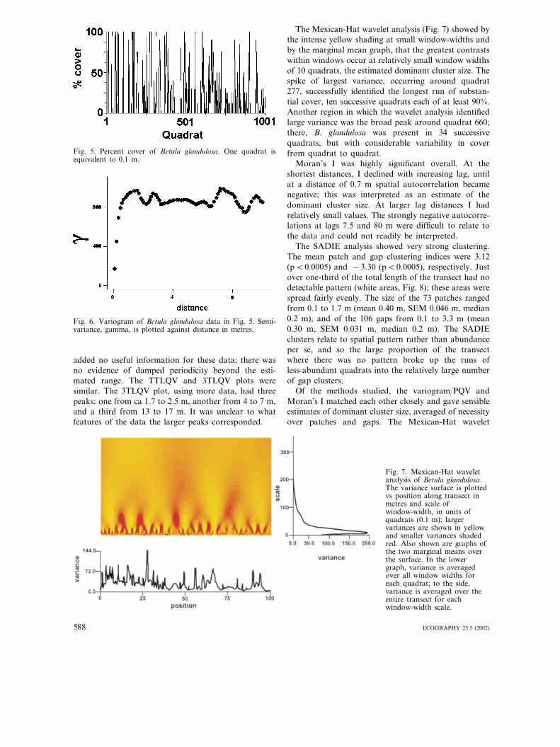
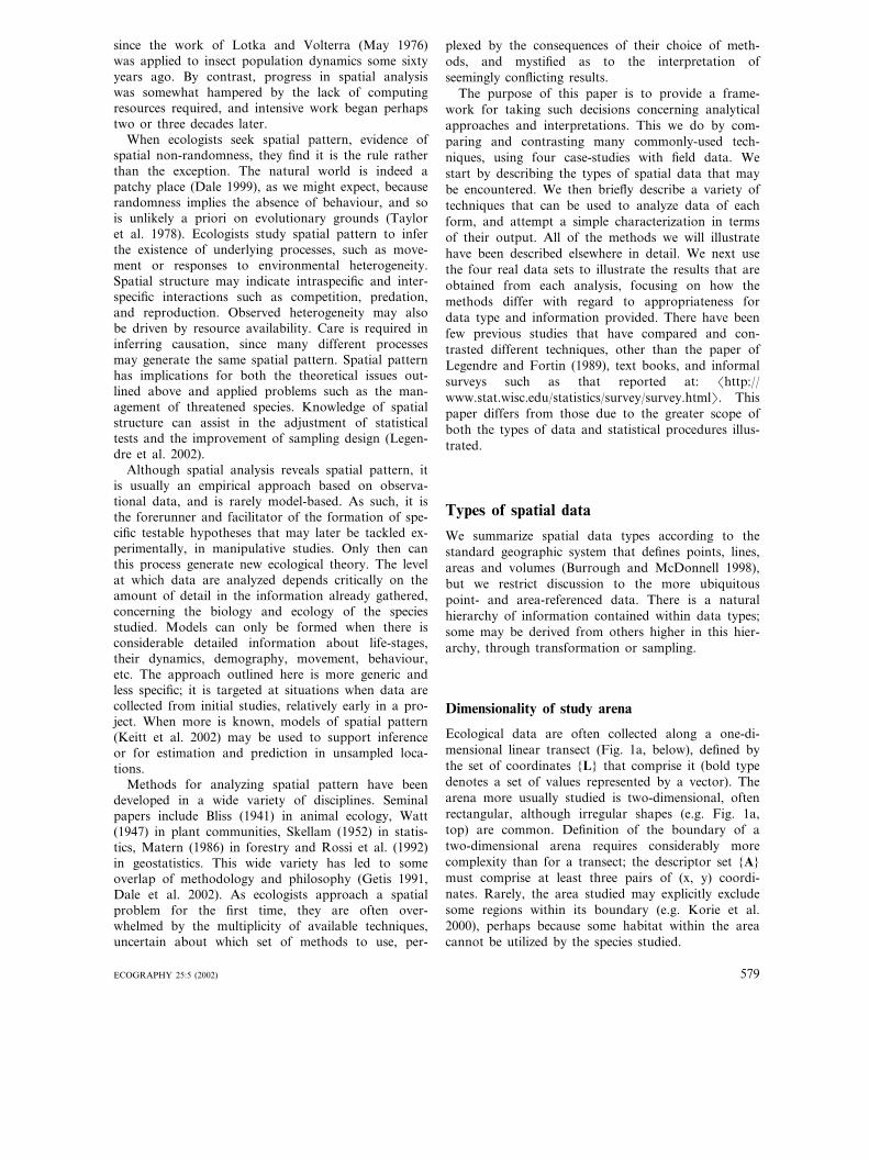
Fig. 5. Percent cover of Betula glandulosa. One quadrat isequivalent to 0.1 m.

The Mexican-Hat wavelet analysis (Fig. 7) showed bythe intense yellow shading at small window-widths andby the marginal mean graph, that the greatest contrastswithin windows occur at relatively small window widthsof 10 quadrats, the estimated dominant cluster size. Thespike of largest variance, occurring around quadrat277, successfully identified the longest run of substan-tial cover, ten successive quadrats each of at least 90%.Another region in which the wavelet analysis identifiedlarge variance was the broad peak around quadrat 660;there, B. glandulosa was present in 34 successivequadrats, but with considerable variability in coverfrom quadrat to quadrat.

Moran’s I was highly significant overall. At theshortest distances, I declined with increasing lag, untilat a distance of 0.7 m spatial autocorrelation becamenegative; this was interpreted as an estimate of thedominant cluster size. At larger lag distances I hadrelatively small values. The strongly negative autocorre-lations at lags 7.5 and 80 m were difficult to relate tothe data and could not readily be interpreted.

The SADIE analysis showed very strong clustering.The mean patch and gap clustering indices were 3.12(p�0.0005) and −3.30 (p�0.0005), respectively. Justover one-third of the total length of the transect had nodetectable pattern (white areas, Fig. 8); these areas werespread fairly evenly. The size of the 73 patches rangedfrom 0.1 to 1.7 m (mean 0.40 m, SEM 0.046 m, median0.2 m), and of the 106 gaps from 0.1 to 3.3 m (mean0.30 m, SEM 0.031 m, median 0.2 m). The SADIEclusters relate to spatial pattern rather than abundanceper se, and so the large proportion of the transectwhere there was no pattern broke up the runs ofless-abundant quadrats into the relatively large numberof gap clusters.

Of the methods studied, the variogram/PQV andMoran’s I matched each other closely and gave sensibleestimates of dominant cluster size, averaged of necessityover patches and gaps. The Mexican-Hat wavelet

Fig. 6. Variogram of Betula glandulosa data in Fig. 5. Semi-variance, gamma, is plotted against distance in metres.

added no useful information for these data; there wasno evidence of damped periodicity beyond the esti-mated range. The TTLQV and 3TLQV plots weresimilar. The 3TLQV plot, using more data, had threepeaks: one from ca 1.7 to 2.5 m, another from 4 to 7 m,and a third from 13 to 17 m. It was unclear to whatfeatures of the data the larger peaks corresponded.

Fig. 7. Mexican-Hat waveletanalysis of Betula glandulosa.The variance surface is plottedvs position along transect inmetres and scale ofwindow-width, in units ofquadrats (0.1 m); largervariances are shown in yellowand smaller variances shadedred. Also shown are graphs ofthe two marginal means overthe surface. In the lowergraph, variance is averagedover all window widths foreach quadrat; to the side,variance is averaged over theentire transect for eachwindow-width scale.

588 ECOGRAPHY 25:5 (2002)

Fig. 8. SADIE analysis ofBetula glandulosa. Red shadingindicates patches with clusterindex values �1.5; blueshading indicates gaps withindex values � −1.5; whiteareas represent lengths that areneither patches nor gaps.

provided a larger estimate, but gave very useful insightsinto other aspects of the data. TTLQV and 3TLQVperformed poorly, and added no extra useful interpre-tation. The SADIE method provided separate and dif-ferent estimates of patch and gap size, which weresensible.

Picea glauca

The observed Picea glauca data exhibited a small num-ber of relatively small patches (Fig. 9a), having similarstructure to the Betula data above, but of a muchsparser nature. There were 20 small bursts of cover,ranging from 0.1 to 1 m with mean length 0.24 m. Lessthan 5% of quadrats were occupied and the runs con-taining no Picea ranged up to 18.1 m with mean length4.54 m.

The PQV (Fig. 10, top) implied an average clustersize of 1.1 m, although for situations where the ob-served patch and gap size are as disparate as here thishas little interpretive utility. Its interesting feature was asudden decline in variance at around 10.5 m, unusualfor a PQV/variogram, and caused by the sparseness ofthe data. This distance was highlighted because it repre-sented roughly the minimum between any of the fourpatches containing at least one quadrat with �80%cover shown in Fig. 9a. At shorter distances, variancewas dominated by the comparison between those pairsof quadrats, one of which contained a member of oneof these four patches and the other of which did not.The upward slope over long stretches of the plot indi-cated the clear trend in the data. The TTLQV and3TLQV plots showed no sudden decline in variance;

they indicated structure with an average cluster size ca6 m and ca 3.8 m, respectively.

Marginal variance in the Mexican-Hat wavelet plotmirrored the positions of the four largest patches re-ferred to above, but showed little further structure;marginal variance was maximal at 0.9 m.

Usually, Geary’s c and Moran’s I (Fig. 10, middleand below) are very similar except for inversion, but forthese data they differed. Both indicated an dominantaverage cluster size of 0.9 m, but whereas I remainedfairly flat thereafter, c continued to increase beforecrossing the x-axis again around 10.5 m, informativelyindicating a second scale of pattern at the same distanceas found by PQV (Fig. 10, top).

The SADIE analysis confirmed substantial spatialpattern, the mean clustering indices for patches being3.25 (p�0.0013) and for gaps −3.88 (p�0.0013). Aproportion of 0.29 of the total length of the transecthad no detectable pattern, almost all within the left-hand half of the transect. The 19 patches were correctlyidentified, ranging in size from 0.1 to 0.5 m (mean 0.18m, SEM 0.031 m, median 0.1 m), and the 43 gaps from0.1 to 12.7 m (mean 1.6 m, SEM 0.36 m, median 0.8m).

Salix glauca

Data for Salix glauca was similar in structure to bothother species. There was considerable spatial pattern,with a degree of sparseness midway between the othertwo species (Fig. 9b). No feature of any analyses wasfundamentally different from those discussed above, sonone is reported, but the data are presented to inform

Fig. 9. Percent cover of (a)Picea glauca and (b) Salixglauca. One quadrat isequivalent to 0.1 m.

ECOGRAPHY 25:5 (2002) 589

Fig. 10. Methods that measure variability plotted againstvarying extents in units of metres (ten quadrats) for Piceaglauca. Above is local paired quadrat variance, PQV; under-neath are two correlograms, Moran’s I (middle graph) andGeary’s c (lower graph). Filled symbols indicate significantindividual lags (p�0.05).

Cross-correlograms and cross-variograms also revealedlittle structure.

However, SADIE analysis of the cluster indices re-vealed strongly significant positive association betweenthe spatial pattern in pairs of all three species (Betulaglandulosa and Picea glauca, X=0.244, p�0.001; Be-tula glandulosa and Salix glauca, X=0.133, p=0.001;Picea glauca and Salix glauca, X=0.401, p�0.001).The method of Clifford et al. (1989) suggested anapproximate halving of the effective degrees of freedomfor each species pair; probability levels and confidencelimits, from randomizations under the null hypothesisof no association, were adjusted accordingly. In a mapof local association, �k, for Picea glauca and Salixglauca (Fig. 11), the dominance of plum shading overgreen demonstrates an overall positive association be-tween the species. The positions of the shaded contoursdistinguishes areas in which relatively large local valuesoccurred. For example, the plum shading betweenquadrats 333 and 336 reflects values of positive localassociation, arising from the coincidence of patchesexceeding 40% cover for both species. Detrending thecluster indices by a quadratic function suggested thatthe association found was due mainly to larger-scalesimilarities between the species. All maps showed con-siderable clustering of local association towards theextreme right of the transect, where the coincidences ofseveral gaps reflected long runs of quadrats where coverwas exceedingly sparse or absent for all species.

The difference between the results for the simplecorrelation analyses and SADIE arise, as for the singlespecies comparisons, because the former makes com-parisons between variables that are abundance/densityestimates, where an isolated large value contributesequally to the computed statistic as does a similar valuein a patch. By contrast, the SADIE analysis is basedupon the degree of spatial pattern, so isolated valuesare deliberately downweighted.

the analysis of relationships between the species, dis-cussed below.

Relationships between the speciesUsing the raw cover data, correlations between speciespairs were small (Betula glandulosa and Picea glauca,r=0.0188; Betula glandulosa and Salix glauca, r=−0.0577; Picea glauca and Salix glauca, r=0.0016).None was significant, before or after accounting forspatial structure using the Clifford et al. (1989) method.

Fig. 11. SADIE localassociation (y-axis), �k,between Picea glauca andSalix glauca versus position ofkth quadrat (x-axis). Symbolsdenote values of �k exceedingupper or lower critical values(25 expected); 35 filled plumcircles indicate significantpositive association, singleopen green symbol indicatesnegative dissociation. Variationof local association alongtransect is shown, for allvalues of �k, by shaded bandsof colour in rectangle (plumpositive; green negative; darkershades indicate greaterextremes of association).

590 ECOGRAPHY 25:5 (2002)

Fig. 12. (a) Locations ofthe 4357 Ambrosiadumosa individuals in the100×100 m study arena.(b) Frequencydistribution of the countof individuals per 5×5m subarea quadrat.

Case study 2: mapped locations and volume of adesert shrub

The data (Miriti et al. 1998) are the locations andlogarithmically-transformed estimated plant canopyvolumes of all individual adults of the deciduous desertshrub Ambrosia dumosa, recorded on a single occasionin a 100×100 m area in the Colorado Desert (Wrightand Howe 1987). These data form a subset of a largerand phased study of plant dynamics with different lifestages, in which Ambrosia dumosa encompassed almosttwo-thirds of all recorded stems. The study site wasselected deliberately to minimize heterogeneity at-tributable to environmental variation. Miriti et al.(1998), and see references within) were interested in therelative importance and effects of possible intra-specificinterference and negative plant-to-plant interactions onspatial distribution, and to quantify the spatial scales

over which major processes operated. Here, four ver-sions of the data were analyzed: (x, y) point locations,derived (x, y, z) counts in 5×5 m contiguous subareas,(z) attributes (nearest neighbour distances and vol-umes), and derived (x, y, z) mean volume per plant in5×5 m contiguous subareas.

Individuals of A. dumosa seemed to be distributedthroughout the study arena with considerable, butsmall-scale aggregation (Fig. 12a). Two or three bandsof relatively low or zero density, of width ca 15 m,appeared to run roughly north-west to south-eastacross the area. The frequency distribution of countsper 5×5 m quadrat shows a typically right-skeweddistribution with a mean of 10.86 plants per quadratand a similar mode (Fig. 12b); the variance/mean ratiowas 4.3, which indicates significant numerical varianceheterogeneity.

Fig. 13. Ripley’s L� (t) functionfor Ambrosia dumosaindividuals, where t representsthe radius in metres of thenotional circle drawn around arandomly chosen plant. Alsoshown are upper, Ru(t) andlower, Rl(t) envelopesrepresenting upper 97.5%-ilesand lower 2.5%-iles under thenull hypothesis of completespatial randomness, derivedfrom Monte Carlorandomizations. Here, forvisual clarity, the threey-variables are eachtransformed by subtracting t,prior to plotting: L� (t) – t arefilled circles, Ru(t) – t areopen triangles, Rl(t) – t areopen diamonds. The x-axisrepresents t. Filled circlesabove the upper envelopeindicate significant aggregationand those below the lowerenvelope indicate significantregularity.

ECOGRAPHY 25:5 (2002) 591

Fig. 14. Semivariance from directional variograms for Am-brosia dumosa counts, in 5×5 m quadrats, plotted againstdistance in metres, in directions: 0°, 45°, 90° and 135°.

as data the counts of individuals within contiguous 2n

m2 square subareas, where n=2, 3, and upwards. Thisgave an initial, rough indication of the relationship ofhow aggregation varied with subarea size. It showedmoderate and non-significant heterogeneity, but whichcrucially decreased monotonically with subarea fromthe smallest, with side 2 m, and became virtually indis-tinguishable from random at the largest tested, withside 11.3 m. Hence, both these results confirmed theconclusions of Miriti et al. (1998) and the visual impres-sion from Fig. 12a. There was considerable aggregationat the smallest spatial extents, consistent with someunspecified plant-to-plant interactions, but this seemedto decrease over medium extents of ca 100 m2 with sidesof 10 m, a distance beyond which an individual plantwould expect to exert an influence over others.

To quantify further the relationship between aggrega-tion and spatial scale of distance, t, we plotted Ripley’sL� (t) function versus t for the (x, y) point location data(Fig. 13). This confirmed one indication from theblocked quadrat variance analysis, that there was sig-nificant and strong aggregation from the smallest scalestudied, a distance of 0.7 m, which declined almostmonotonically with t. However, this did not cross theupper envelope until ca 24 m. Unusually, L� (t) contin-ued to decline, indicating regularity by falling substan-tially below the lower envelope, and not until 60 m did

Previous analyses by Miriti et al. (1998) showed thatthe total nearest neighbour distance was 386.0, whichexceeded the expectation for a random distribution,using Donnelly’s (1978) method, by over 15 times thestandard deviation, indicating highly significant aggre-gation. They also used a hierarchical blocked quadratvariance method (Dale 1999), based on Morisita’s(1959) index (the test for which is equivalent to Greig-Smith’s (1952) test of the index of dispersion I), using

Fig. 15. Overlaid contour andclassed post maps of SADIEclustering indices for counts ofAmbrosia dumosa, in 5×5 mquadrats. Red shading anddarker, larger filled red circlesindicate strong patchiness withindex values �1.5; blueshading and darker, largerfilled blue circles indicatestrong gaps with index values� −1.5. Medium-sized filledcircles: units with clusteringthat exceeds expectation (�1or � −1). Open circles:clustering below expectation(�1 or � −1).

592 ECOGRAPHY 25:5 (2002)

Fig. 16. Frequency distribution of Ambrosia dumosa logarith-mically-transformed plant canopy volume per plant.

ensures that there is considerable autocorrelation in theplot of L� (t) vs t. Hence, it would not only be unwise toinfer that true regularity existed at the scale of 60 m,but also to infer that the distance at which the spatialprocess became random was 24 m, or indeed to attempta precise estimate of this distance. In summary, themost important information conveyed by this analysisrelates to the existence of the strongest pattern at thesmallest distances.

The following analyses were done for the counts ofindividuals in 5×5 m contiguous subareas. Directionalvariograms were calculated (Fig. 14). The large nuggetvariance and shallow slope up to the sill supported theconclusion above, that the major structure in the dataoccurred at distances smaller than were resolvable bythe subarea size. The variogram range also confirmedthe indication, from L� (t), that there was some larger-scale structure up to distances of ca 25 m. This distancewas confirmed by the results from both Moran’s I andGeary’s c. Additionally, the variograms showed somemild anisotropy in the 135° direction for distances �40m, providing further support for the existence of thebands referred to above, although no directionality wasdetected by an angular correlation analysis.

The SADIE analysis confirmed the presence of large-scale patches of varying size up to ca 400 m2 (meanpatch cluster index=1.29; p=0.025), and gaps (meangap cluster index= −1.35; p=0.048). The most nota-ble feature was a long gap ca 10 m wide stretching fromleft to right across almost the entire width of thehectare block (Fig. 15), and supporting further theexistence of the bands of low density.

it increase again relative to the randomizations. This isnot thought to reflect an important facet of the data. Itwas probably a manifestation of the change in intensityalong the diagonal that runs from lower-left to upper-right of the area, which appears to cycle 2.5 times as ittraverses the two large relatively empty bands referredto above. The wavelength of this cycle is ca (40�2)m=57 m which coincides well with the value of t forwhich L� (t) is a minimum. The abundance of individuals

Fig. 17. (a) The 100×100grid of NDVI derived fromAVHRR data from 7 to 20August, 1992, collected overthe Cascade Mountains.Darker shades representsmaller values. (b) The100×100 grid of elevationdata from the same location.(c) Frequency distribution ofNDVI and (d) elevation infeet.

ECOGRAPHY 25:5 (2002) 593

Fig. 18. (a) Moran’s I correlogram for NDVI; all lags are significant (p�0.05). (b) Angular correlation for NDVI. (c)Directional variogram for NDVI and (d) elevation.

There was a very strong linear relationship betweenlogarithmically-transformed plant canopy volume andcounts, and when mapped these two derived (z) vari-ables appeared very similar. However, a frequency dis-tribution of transformed volume per plant (Fig. 16)showed a clearly bimodal distribution with relativelymany plants in the smallest size class and a secondmore symmetric mode for much larger plants. Suchbimodality is characteristic of many long-lived plants inwhich seeds readily germinate, but mortality of smallerindividuals is high until a certain size threshold isreached, after which survival probabilities increase untilsenescence. Also, mapping revealed considerable spatialpattern in the values of volume per plant within the5×5 m contiguous subareas. Broadly, volumes perplant were greater in the left-hand half of the studyarena (x�50, mean transformed volume per plant=12.93 with SEM 0.121; x�50, mean transformed vol-ume per plant=12.42 with SEM 0.099). Clustering wassignificant (SADIE indices both p=0.0002), with tworegions of relatively low volume per plant (top centreand lower-right side, each 200–300 m2) and one 200 m2

patch of greater than average volume, at the lower-leftof the area. The reason for spatial structure in thesegrowth differences between plants is unknown.

Case study 3: remotely-sensed AVHRR data inthe Cascade Mountains

Since 1982, the Advanced Very High-Resolution Ra-diometer (AVHRR) satellite imager (Eidenshink 1992)has collected image data from daily coverage of theEarth, using a nominal 1-km sampling rate. We down-loaded archived and processed area-referencedAVHRR data, collected from 7 to 20 August 1992,from the EROS Data Center web site �http://edcwww.cr.usgs.gov/landdaac/1KM/comp10d.html�.We extracted a 100×100 matrix of ca 1 km square cellslocated on the east side of the Northern CascadeMountains, Washington (Fig. 17a). The normalizeddifference vegetation index (NDVI) (James and Kalluri1993, Townshend et al. 1994), the difference of near-in-frared (channel 2) and visible (channel 1) reflectancedivided by their sum, were also provided. Positivevalues of NDVI indicate green vegetation; negativevalues indicate non-vegetated surface features such aswater, barren rock, ice, snow or clouds. To minimizedata storage requirements, NDVI values were rescaledas integers in the interval [0,200]. A US GeologicalSurvey digital elevation model from the same region(e.g. Thelin and Pike 1991) was registered with the

594 ECOGRAPHY 25:5 (2002)

NDVI data and resampled to the same 1×1 km gridcells (Fig. 17b). Frequency distributions for NDVI (Fig.17c) and elevation (measured in feet, Fig. 17d) exhib-ited only slight skewness and no transformation wasneeded before analysis. Specific questions posed forthese data were: what are the spatial patterns of NDVIand elevation and how similar are they? Are these twovariables correlated?

Declining values in Moran’s I correlogram (Fig. 18a)and increasing values in the directional variogram (Fig.18c) indicated strong, positive autocorrelation in vege-tation across the map, while their monotonic natureacross the full range of distances indicated the presenceof a large-scale trend or gradient of vegetation. Thistrend was present in every direction except for a 45°angle. The angular correlation diagram (Fig. 18b) con-firmed this directionality, achieving maximal values be-tween 90° and 135°. This revealed anisotropy may beseen clearly in the raw data (Fig. 17a); highest NDVIvalues are to the north-west and lowest values to thesouth-east. This pattern probably reflects the distribu-tion of forested areas along the eastern slope of theNorth Cascade Mountains. Forests are more abundantat higher elevations and high desert vegetation is domi-nant at the lower elevations to the south-west. Thecorrelogram, angular correlation diagram and an-isotropy directions for elevation were so similar tothose for NDVI that they are not shown. The direc-tional variogram for elevation (Fig. 18d) confirms theanisotropy shown by the trend and direction of thestrongest gradient evident in the map (Fig. 17b).

Rossi et al. (1992) pointed out that a large-scaletrend, such as the anisotropy found here for NDVI andelevation, could obscure patterns of spatial dependenceat smaller lag distances. Here, it is unclear from thedirectional variograms (Fig. 18c, d) whether anisotropy

exists in autocorrelation at short lag distances or islimited to the large-scale trend.

In order to investigate further the scale of autocorre-lation and anisotropy, we removed the large-scale trendin both data sets by fitting a model of the form:zx,y=a+b1x+b2y. Estimates of the parameters forNDVI were: a= −172.4, b1= −0.000173, b2=0.000107; and for elevation: a= −55119, b1=−0.0303, b2=0.0258. The directional variograms forthe detrended NDVI residuals from this model (Fig.19a) differed from those discussed above; they reacheda maximum (sill), and indicated less anisotropy, al-though the range appeared slightly longer in the 135°direction than for other angles. The directional vari-ograms of the detrended elevation data (Fig. 19b)showed precisely the same differences, but additionally,for the 90° angle the elevation variogram exhibited aslight ‘‘hole effect’’, first increasing then decreasing withincreasing lag distances. This pattern is characteristic ofsome sort of oscillatory undulation or repetitive fluctu-ation (Isaaks and Srivastava 1989) here probablycaused by the regular alternation of valleys and ridges.The same pattern also appears, although less distinctly,in the 90° variogram (Fig. 19a) of the NDVI data.

Overall, there was a striking similarity between theNDVI and elevation variograms. Both had nugget ef-fects near zero for the raw data, indicating the existenceof a very continuous, smooth surface. The ranges ofboth detrended sets of data were between 10 000 and20 000 m, presumably reflecting the average distancebetween mountain peaks. However, the similarity of thevariograms cannot be used alone to infer their associa-tion, since many different spatial arrangements mayshare the same variogram (Liebhold and Sharov 1998).We calculated a Pearson correlation coefficient of0.4916 between raw NDVI and elevation; a ‘‘naıve’’ test

Fig. 19. Directional variograms of detrended data. (a) NDVI, (b) elevation.

ECOGRAPHY 25:5 (2002) 595

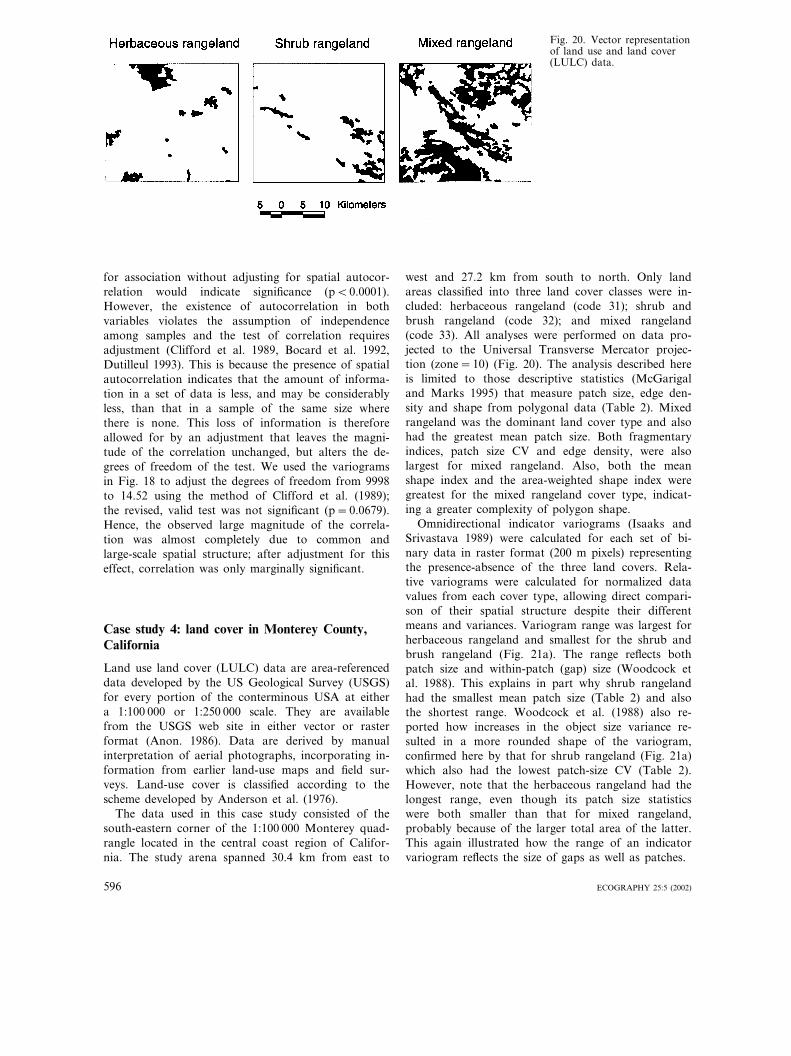
Fig. 20. Vector representationof land use and land cover(LULC) data.

for association without adjusting for spatial autocor-relation would indicate significance (p�0.0001).However, the existence of autocorrelation in bothvariables violates the assumption of independenceamong samples and the test of correlation requiresadjustment (Clifford et al. 1989, Bocard et al. 1992,Dutilleul 1993). This is because the presence of spatialautocorrelation indicates that the amount of informa-tion in a set of data is less, and may be considerablyless, than that in a sample of the same size wherethere is none. This loss of information is thereforeallowed for by an adjustment that leaves the magni-tude of the correlation unchanged, but alters the de-grees of freedom of the test. We used the variogramsin Fig. 18 to adjust the degrees of freedom from 9998to 14.52 using the method of Clifford et al. (1989);the revised, valid test was not significant (p=0.0679).Hence, the observed large magnitude of the correla-tion was almost completely due to common andlarge-scale spatial structure; after adjustment for thiseffect, correlation was only marginally significant.

Case study 4: land cover in Monterey County,California

Land use land cover (LULC) data are area-referenceddata developed by the US Geological Survey (USGS)for every portion of the conterminous USA at eithera 1:100 000 or 1:250 000 scale. They are availablefrom the USGS web site in either vector or rasterformat (Anon. 1986). Data are derived by manualinterpretation of aerial photographs, incorporating in-formation from earlier land-use maps and field sur-veys. Land-use cover is classified according to thescheme developed by Anderson et al. (1976).

The data used in this case study consisted of thesouth-eastern corner of the 1:100 000 Monterey quad-rangle located in the central coast region of Califor-nia. The study arena spanned 30.4 km from east to

west and 27.2 km from south to north. Only landareas classified into three land cover classes were in-cluded: herbaceous rangeland (code 31); shrub andbrush rangeland (code 32); and mixed rangeland(code 33). All analyses were performed on data pro-jected to the Universal Transverse Mercator projec-tion (zone=10) (Fig. 20). The analysis described hereis limited to those descriptive statistics (McGarigaland Marks 1995) that measure patch size, edge den-sity and shape from polygonal data (Table 2). Mixedrangeland was the dominant land cover type and alsohad the greatest mean patch size. Both fragmentaryindices, patch size CV and edge density, were alsolargest for mixed rangeland. Also, both the meanshape index and the area-weighted shape index weregreatest for the mixed rangeland cover type, indicat-ing a greater complexity of polygon shape.

Omnidirectional indicator variograms (Isaaks andSrivastava 1989) were calculated for each set of bi-nary data in raster format (200 m pixels) representingthe presence-absence of the three land covers. Rela-tive variograms were calculated for normalized datavalues from each cover type, allowing direct compari-son of their spatial structure despite their differentmeans and variances. Variogram range was largest forherbaceous rangeland and smallest for the shrub andbrush rangeland (Fig. 21a). The range reflects bothpatch size and within-patch (gap) size (Woodcock etal. 1988). This explains in part why shrub rangelandhad the smallest mean patch size (Table 2) and alsothe shortest range. Woodcock et al. (1988) also re-ported how increases in the object size variance re-sulted in a more rounded shape of the variogram,confirmed here by that for shrub rangeland (Fig. 21a)which also had the lowest patch-size CV (Table 2).However, note that the herbaceous rangeland had thelongest range, even though its patch size statisticswere both smaller than that for mixed rangeland,probably because of the larger total area of the latter.This again illustrated how the range of an indicatorvariogram reflects the size of gaps as well as patches.

596 ECOGRAPHY 25:5 (2002)

Directional variograms for shrub rangeland (Fig.21b) demonstrated anisotropy; the range was consider-ably longer in the north and northwest directions. Thisdifference appeared to reflect both an elongation ofpatches in a consistent north-westerly direction, as wellas the arrangement of patches along a band running inthat same direction (Fig. 20). This anisotropy probablyreflects ridge topography that may be associated withvegetation. The hole effect (depression at ca 2300 m) inthe north-east directional variogram (Fig. 21b) reflectedthe alternating presence and absence encountered whentraversing the study arena in a direction perpendicularto the angle of patch elongation (Fig. 20).

Discussion

We have attempted to offer, for a limited number ofsets of data, some flavour of the kinds of outputs,inferences and interpretations possible from spatialanalysis. Readers must realize that we have not at-tempted an exhaustive account. Many methods arecapable of extension to provide further features, tomeet specific needs. For example, almost all of the localquadrat variance methods detect the average size ofpatches and gaps in a phased pattern along a transect,but new local variance (Galiano 1982) detects the sizeof the smallest phase of the pattern, whether it bepatches or gaps. This, when combined with other localquadrat variance methods, allows separate estimationof patch and gap size.

We give only four recommendations to ecologistswith spatial data in search of methods with which toanalyze them. First, make extensive use of simple visu-alization techniques such as graphs and mapping (Tufte1997, Carr 1999) as a first step to understanding spatialcharacteristics in the data. Second, select statisticalmethods that are available and appropriate for the datatype. Third, select a method that can answer pertinentquestions and provide relevant spatial information.Reference to Table 1 may help the selection process.Given the suitability of several methods, it would beinvidious and naıve to attempt to go beyond this torecommend which single specific technique to use.Readers must form their own conclusions, informed bythe theoretical properties of the methods and theirperformance in the above case studies. Most methodsare distinct and no single one can identify all of thespatial characteristics in data. Therefore, our fourthrecommendation is to employ several different tech-niques. We do not believe that any methods we haveexamined intrinsically provide redundant information,fail to detect real patterns, or identify patterns that arenot real.

In certain circumstances, it may be sensible to widenthe possible range of techniques that may be brought tobear on a problem, by converting between data types.

ECOGRAPHY 25:5 (2002) 597

Tab

le2.

Sum

mar

yst

atis

tics

for

the

land

use

and

land

cove

rda

ta,

base

don

desc

ript

ors

ofpa

tche

s,ed

ges

and

shap

efo

rpo

lygo

nal

data

desc

ribi

nghe

rbac

eous

,sh

rub

and

mix

edra

ngel

ands

.

Lan

dty

pe%

ofP

atch

size

Mea

npa

tch

Edg

ede

nsit

yN

umbe

rof

Tot

aled

geP

atch

size

Are

a-w

eigh

ted

Mea

nsh

ape

size

(ha)

patc

hes

leng

th(m

)to

tal

area

(mha

−1)

mea

nsh

ape

coef

ficie

ntof

inde

xst

anda

rdde

viat

ion

(ha)

vari

atio

nin

dex

Her

bace

ous

rang

elan

d7.

346

9.5

1387

5.9

186.

514

000

01.

71.

591.

9Sh

rub

rang

elan

d5.

224

3.6

1833

0.6

135.

717

700

02.

11.

632.

2M

ixed

rang

elan

d36

.814

04.1

2230

90.8

220.

167

620

08.

11.

974.

6

Fig. 21. (a) Omnidirectional relative variograms for LULC data, with semivariance plotted against lagged distance; (b)directional variograms for the shrub and brush rangeland data in (a).

Examples are the formation of counts by conversion ofdata from point locations to contiguous subareas, thetaking of samples, and transformation from polygonalto contiguous subareas (i.e. vector to raster format).For the first two the degree of loss of information mustbe considered (Dungan et al. 2002). For the third, notethat both geographic entities and fields can be repre-sented either in vector (represented by origin, lengthand direction), raster (regular tessellation with squareelements) or TIN (irregular tessellation with triangularelements) form. The choice of form depends largely onthe application of the data (Burrough and McDonnell1998). The vector form assures better accuracy andefficient data storage, while raster data can be pro-cessed faster and are adapted easily to deal withchanges in modes of analysis. Conversion of polygonaldata from vector to raster form was illustrated in casestudy 4. Indeed, the raster format is exploited increas-ingly as the primary data type in landscape ecology,because of the growing utilization of remotely-senseddata in that discipline (and see case study 3, above).The conversion facilitated the application of a widerrange of statistical methods, such as indicator vari-ograms, frequently used in disciplines other than land-scape ecology. A further example of the generic use ofstatistical techniques is the texture and ‘‘lacunarity’’measures employed in remote sensing and landscapeecology (Plotnick et al. 1993), that calculate varianceacross gliding windows. Dale et al. (2002) note theirsimilarity to the local quadrat variance methods used inplant ecology.

Acknowledgements – This work was conducted as part of the‘‘Integrating the Statistical Modeling of Spatial Data in Ecol-ogy’’ Working Group supported by the National Center forEcological Analysis and Synthesis (NCEAS). NCEAS is acenter funded by the NSF (Grant cDEB-94-21535) of theUSA, the Univ. of California-Santa Barbara, the CaliforniaResources Agency, and the California Environmental Protec-tion Agency. IACR-Rothamsted receives grant-aided supportfrom the Biotechnology and Biological Sciences ResearchCouncil of the U.K.

ReferencesAnderson, J. R. et al. 1976. A land use and land cover

classification system for use with remote sensor data. –U.S. Geol. Surv., Prof. Pap. 964.

Anon 1986. Land use land cover digital data from 1:250 000and 1:100 000-scale maps, data user guide 4. – U.S. Geol.Surv.

Anselin, L. 1995. Local indicators of spatial association –LISA. – Geogr. Anal. 27: 93–115.

Bailey, R. G. and Ropes, L. 1998. Ecoregions: the ecosystemgeography of the oceans and continents. – Springer.

Bjørnstad, O. N., Ims, R. A. and Lambin, X. 1999. Spatialpopulation dynamics: analyzing patterns and processes ofpopulation synchrony. – Trends Ecol. Evol. 14: 427–431.

Bliss, C. I. 1941. Statistical problems in estimating populationsof Japanese beetle larvae. – J. Econ. Entomol. 34: 221–232.

Bocard, D., Legendre, P. and Drapeau, P. 1992. Partiallingout the spatial component of ecological variation. – Ecol-ogy 73: 1045–1055.

Bradshaw, G. A. and Spies, T. A. 1992. Characterizing canopygap structure in forests using wavelet analysis. – J. Ecol.80: 205–215.

Burrough, P. A. and McDonnell, R. A. 1998. Principles ofgeographical information systems. – Oxford Univ. Press.

Carr, D. B. 1999. New templates for environmental graphics:from micromaps to global grids. – Proc. of the 9th LukacsSymp., Bowling Green State Univ., Bowling Green, Ohio,USA, 23–25 April.

Chatfield, C. 1985. The initial examination of data. – J. R.Stat. Soc. A 148: 214–253.

Clark, P. J. and Evans, F. C. 1954. Distance to nearestneighbour as a measure of spatial relationships in popula-tions. – Ecology 35: 23–30.

Cliff, A. D. and Ord, J. K. 1973. Spatial autocorrelation. –Pion.

Cliff, A. D. and Ord, J. K. 1981. Spatial processes: models andapplications. – Pion.

Clifford, P., Richardson, S. and Hemon, D. 1989. Assessingthe significance of the correlation between two spatialprocesses. – Biometrics 45: 123–134.

Cressie, N. A. C. 1991. Statistics for spatial data. – Wiley.Dale, M. R. T. 1999. Spatial pattern analysis in plant ecology.

– Cambridge Univ. Press.Dale, M. R. T. and Zbigniewicz, M. W. 1997. Spatial pattern

in boreal shrub communities: effects of a peak in herbivoredensities. – Can. J. Bot. 75: 1342–1348.

Dale, M. R. T. and Mah, M. 1998. The use of wavelets forspatial pattern analysis in ecology. – J. Veg. Sci. 9: 805–814.

598 ECOGRAPHY 25:5 (2002)

Dale, M. R. T. et al. 2002. Conceptual and mathematicalrelationships among methods for spatial analysis. – Ecog-raphy 25: 558–577.

David, F. N. and Moore, P. G. 1954. Notes on contagiousdistributions in plant populations. – Ann. Bot. Lond. 18:47–53.

Diggle, P. J. 1983. Statistical analysis of spatial point patterns.– Academic Press.

Donnelly, K. P. 1978. Simulations to determine the varianceand edge-effect of total nearest neighbor distance. – In:Hodder, I. (ed.), Simulation studies in archaeology. Cam-bridge Univ. Press, pp. 91–95.

Dungan, J. et al. 2002. A balanced view of scale in spatialstatistical analysis. – Ecography 25: 626–640.

Dutilleul, P. 1993. Modifying the t-test for assessing the corre-lation between two spatial processes. – Biometrics 49:305–314.

Eidenshink, J. C. 1992. The 1990 conterminous U.S. AVHRRdata set. – Photo. Engin. Rem. Sens. 58: 809–813.

Falsetti, A. B. and Sokal, R. R. 1993. Genetic structure ofhuman populations in the British Isles. – Ann. HumanBiol. 20: 315–329.

Fisher, R., Thornton, H. and Mackenzie, W. 1922. The accu-racy of the plating method of estimating the density ofbacterial populations. – Ann. Appl. Biol. 9: 325–359.

Galiano, E. F. 1982. Detection et mesure de l’heterogeneitespatial des especes dans les paturages. – Acta Oecol.Oecol. Plant. 3: 269–278.

Getis, A. 1991. Spatial interaction and spatial autocorrelation:a cross-product approach. – Environ. Plann. A 23: 1269–1277.

Getis, A. and Ord, J. K. 1995. The analysis of spatial associa-tion by use of distance statistics. – Geogr. Anal. 24:189–206.

Greig-Smith, P. 1952. The use of random and contiguousquadrats in the study of the structure of plant communi-ties. – Ann. Bot. 16: 293–316.

Gustafson, E. J. 1998. Quantifying landscape spatial pattern:what is the state of the art? – Ecosystems 1: 143–156.

Haase, P. 1995. Spatial pattern analysis in ecology based onRipley’s K-function: introduction and methods of edgecorrection. – J. Veg. Sci. 6: 575–582.

Hanski, I. A. and Gilpin, M. E. 1997. Metapopulation biol-ogy: ecology, genetics and evolution. – Academic Press.

Hassell, M. P., Comins, H. and May, R. M. 1991. Spatialstructure and chaos in insect population dynamics. – Na-ture 353: 255–258.

Hurlbert, S. 1990. Spatial distribution of the montane unicorn.– Oikos 58: 257–271.

Isaaks, E. H. and Srivastava, R. M. 1989. An introduction toapplied geostatistics. – Oxford Univ. Press.

James, M. E. and Kalluri, S. 1993. The pathfinder AVHRRland data set: an improved coarse resolution data set forterrestrial monitoring. – The Int. J. Rem. Sens. 15: 3347–3364.

Jumars, P. A., Thistle, D. and Jones, M. L. 1977. Detectingtwo-dimensional spatial structure in biological data. –Oecologia 28: 109–123.

Keitt, T. et al. 2002. Accounting for spatial pattern whenmodeling organism-environment interactions. – Ecography25: 616–625.

Korie, S. et al. 1998. Analysing maps of dispersal around asingle focus (with Discussion). – Ecol. Environ. Stat. 5:317–350.

Korie, S. et al. 2000. Spatiotemporal associations in beetle andvirus count data. – J. Agricult. Biol. Environ. Stat. 5:214–239.

Legendre, P. and Fortin, M.-J. 1989. Spatial pattern andecological analysis. – Vegetatio 80: 107–138.

Legendre, P. et al. 2002. The consequences of spatial structurefor the design and analysis of ecological field surveys. –Ecography 25: 601–615.

Liebhold, A. M. and Sharov, A. A. 1998. Testing for correla-tion in the presence of spatial autocorrelation in insectcount data. – In: Baumgartner, J., Brandmayr, P. andManly, B. F. J. (eds), Population and community ecologyfor insect management and conservation. Balkema, pp.111–117.

Liebhold, A. M., Rossi, R. E. and Kemp, W. P. 1993. Geo-statistics and geographic information systems in appliedinsect ecology. – Annu. Rev. Entomol. 38: 303–327.

Lloyd, M. 1967. Mean crowding. – J. Anim. Ecol. 36: 1–30.Matern, B. 1986. Spatial variation, number 36 in lectures notes

in statistics. – Springer.May, R. M. (ed.) 1976. Theoretical ecology. – Blackwell.McGarigal, K. and Marks, B. J. 1995. FRAGSTATS: spatial

pattern analysis program for quantifying landscape struc-ture. – USDA For. Serv. Gen. Tech. Rep., PNW-GTR-351, USDA For. Serv. Pacific Northwest Res. Stn.

Miriti, M., Howe, H. F. and Wright, S. J. 1998. Spatialpatterns of mortality in a Colorado Desert plant commu-nity. – Plant Ecol. 136: 41–51.

Moran, P. A. P. 1950. Notes on continuous stochastic phe-nomena. – Biometrika 37: 17–23.

Morgan, K. A. and Gates, J. E. 1982. Bird population pat-terns in forest edge and strip vegetation at RemingtonFarms, Maryland. – J. Wildl. Manage. 46: 933–944.

Morisita, M. 1959. Measuring the dispersion and the analysisof distribution patterns. – Mem. Fac. Sci., Kyushu Univ.,Ser. E. Biol. 2: 215–235.

Mugglestone, M. A. and Renshaw, E. 1996. A practical guideto the spectral analysis of spatial point processes. – Comp.Stat. Data Anal. 21: 43–65.

Oden, N. L. 1984. Assessing the significance of a spatialcorrelogram. – Geogr. Anal. 16: 1–16.

Oden, N. L. and Sokal, R. R. 1986. Directional autocorrela-tion: an extension of spatial correlograms in two dimen-sion. – Syst. Zool. 35: 608–617.

Ord, J. K. and Getis, A. 1995. Local spatial autocorrelationstatistics: distributional issues and an application. – Geogr.Anal. 27: 286–306.

Perry, J. N. 1998a. Measures of spatial pattern for counts. –Ecology 79: 1008–1017.

Perry, J. N. 1998b. Measures of spatial pattern and spatialassociation for counts of insects. – In: Baumgartner, J.,Brandmayr, P. and Manly, B. F. J. (eds), Population andcommunity ecology for insect management and conserva-tion. Balkema, pp. 21–33.

Perry, J. N. and Woiwod, I. P. 1992. Fitting Taylor’s powerlaw. – Oikos 65: 538–542.

Perry, J. N. et al. 1999. Red-blue plots for detecting clusters incount data. – Ecol. Lett. 2: 106–113.

Peuquet, D. 1984. A conceptual framework and comparison ofspatial data models. – Cartographica 21: 66–113.

Peuquet, D., Smith, B. and Brogaard, B. 1999. The ontologyof fields. – Rep. of a Specialist Meeting held under theAuspices of the Varenius Project, Bar Harbor, Maine,11–13 June, 1998, �http://www.ncgia.ucsb.edu/�vanzuyle/varenius/ontologyoffields–rpt.html�.

Plotnick, R. E., Gardner, R. H. and O’Neill, R. V. 1993.Lacunarity indices as measures of landscape texture. –Landscape Ecol. 8: 201–211.

Ripley, B. D. 1977. Modelling spatial patterns. – J. R. Stat.Soc. B 39: 172–212.

Ripley, B. D. 1988. Statistical inference for spatial processes. –Cambridge Univ. Press.

Rosenberg, M. S. 2000. The bearing correlogram: a newmethod for analyzing directional spatial autocorrelation. –Geogr. Anal. 32: 267–278.

Rossi, R. E. et al. 1992. Geostatistical tools for modeling andinterpreting ecological spatial dependence. – Ecol.Monogr. 62: 277–314.

Silvertown, J. et al. 1992. Cellular automaton models ofinterspecific competition for space – the effect of patternon process. – J. Ecol. 80: 527–534.

ECOGRAPHY 25:5 (2002) 599

Simon, G. 1997. An angular version of spatial correlations,with exact significance tests. – Geogr. Anal. 29: 267–278.

Skellam, J. G. 1952. Studies in statistical ecology. I. Spatialpattern. – Biometrika 39: 346–362.

Sokal, R. R. and Oden, N. L. 1978. Spatial autocorrelation inbiology. 1. Methodology. – Biol. J. Linn. Soc. 16: 199–228.

Sokal, R. R., Oden, N. L. and Thomson, B. A. 1998a. Localspatial autocorrelation in biological variables. – Biol. J.Linn. Soc. 65: 41–62.

Sokal, R. R., Oden, N. L. and Thomson, B. A. 1998b. Localspatial autocorrelation in a biological model. – Geogr.Anal. 30: 331–354.

Southwood, T. R. E. 1966. Ecological methods. – Methuen.Stoyan, D. and Stoyan, H. 1994. Fractals, random shapes and

point fields, methods of geometrical statistics. – Wiley.Taylor, L. R., Woiwod, I. P. and Perry, J. N. 1978. The

density-dependence of spatial behaviour and the rarity ofrandomness. – J. Anim. Ecol. 47: 383–406.

Thelin, G. P. and Pike, R. J. 1991. Landforms of the contermi-nous United States – a digital shaded-relief portrayal. –USGS.

Townshend, J. R. G. et al. 1994. The 1-km AVHRR globaldata set: needs of the International Geosphere Bio-

sphere Program. – The Int. J. Rem. Sens. 15: 3319–3332.

Tufte, E. R. 1997. Visual explanations: images and quantities,evidence and narrative. – Graphics Press.

Turner, M. G. and Gardner, R. H. 1991. Quantitative meth-ods in landscape ecology. – Springer.

Upton, G. J. G. and Fingleton, B. 1985. Spatial data analysisby example. Vol. 1: point pattern and quantitative data. –Wiley.

ver Hoef, J. M., Cressie, N. A. C. and Glenn-Lewin, D. C.1993. Spatial models for spatial statistics: some unification.– J. Veg. Sci. 4: 441–452.

Watt, A. S. 1947. Pattern and process in the plant community.– J. Ecol. 35: 1–22.

Wiens, J. A. 1989. Spatial scaling in ecology. – Funct. Ecol. 3:385–397.

Winder, L. et al. 2001. Modelling the dynamic spatio-temporalresponse of predators to transient prey patches in the field.– Ecol. Lett. 4: 568–576.

Woodcock, C. E., Strahler, A. H. and Jupp, D. L. B. 1988.The use of variograms in remote sensing: I. Scene modelsand simulated images. – Rem. Sen. Environ. 25: 323–348.

Wright, S. J. and Howe, H. F. 1987. Pattern and mortality inColorado desert plants. – Oecologia 73: 543–552.

ECOGRAPHY 25:5 (2002)600