POST-ENVIRONMENTAL EVALUATION OF

THE RA.J.JAPRABHA DAM IN THAILAND

lHESIS SUB.H1TTED TO

TilE COCHIl\ l l\IVERSITY OF SCIE:\CE Al\1) TECIl:\TOLO(;Y

FOR TIlE AWARD OF THE DEGREE OF

ill nl~lor Q-'f iPITilnsoplI1J 1J II 1£ n.1nnl1tir~s

l'NDEn THE FACl'L TY OF SOCIAL SCIE:\TCES

BY

SUMKIATE Sn.lPATHAR

REG. No. 1734

eNDER TilE Sl'PEnVISIOl\ OF

Prof. (Or.) K.C. SANKARANARA YANAN

DE:,\~, FACTLTY OF SOCIAL SCI ENCES

DF.PARTMENT OF APPLIED ECONOMICS

QIllrhtn CUntttrrsiiu of §rirllrl~ nnD illrrhnnlngu

(Cllrhin682022, ilil'r~tn, lInl'lin I

MAY, 2000

DEPARTMENT .OF APPLIED ECONOMICS COCHIN UNIVERSITY OF SCIENCE AND TECI-I:\"OLOGY

KOCHI· 682022, KERALA, S. I1\DIA

Dr. D. RAJASENAN

Professor & Hcad

Phone: 0484 - 556030 F(Jx 0484 - 532495 E-mail: economy@giasmciOl.vsl~:,:H;: :,'

D81e .....

-@pr-tifiratr

Certified that the doctoral Committee has approved the thesis /01'

submission for the award of the degree of Doctor of Philosophy in Economics lIndcl'

the Faculty of Social Sciences.

Pro.J.(Dr.) K.c. SANKARANARA Y ANAN

Guide

Cochin University of Science and Technology

Cochin 682 022

May, 26, 2000

Ji",,' ~~. Prof. ~ D. RAJASENAN

Do~oral Committee Member

DEPARTMENT .OF APPLIED ECONOI\1ICS COCHIN UNIVERSITY OF SCIENCE AND TECHr\OLOGY

KOCH! - 682022, KEHALA, S. I~DIA

Phone: 0484 - 555030 Dr. K.C SANKARANARA Y ANAN Fax 0484 - 532495

Dean, Faculty of Social Sciences

o. AE. DBIC.

err rrlifi ru le

Certified that the thesis entitled "Post Environmental Evaluation of

the Rajjaprabha Dam in Thailand" is the record of bonafide research corried ()1If

by Mr. SOMKIATE SRIPATHAR under my supervisiol1. The thesis is ll"()uh

submitting for the degree of Doctor (?f Philosophy in Economics under the FacZllty

of So cia I Sciences.

Prof. (Dr.) KC. SAI~:~:;;ARA ~

Cochin University of Science and Technology

Cochin 682 022

May, 26, 2000

Dean, Faculty of Social Sciences

if) £ rlnrntinn

1 declare that this thesis is the record afhanafide research carried

out by me under the supervision of Dr. K.C. SANKARANARAYANAJV,

Professor and farmer Head afthe Department of Applied Economics, and the

Dean, Faculty of Social Sciences, Cochin University of Science and Technology,

Cochin 682022. 1 further declare that this thesis has not prevlOus/yformcd (he

basis of the award of any degree, diploma, associateship, fellows/lip or of her

similar title of recognition.

Cochin University of Science and Technology

Co chin 682022

May, 26, 2000

$0 MAlt!' ~~ ~,../~-.l-k SOMKlATE SRlPATHAR

ACKNOWLEDGEMENT

First and foremost I would like to express my Sll1cere gratitude to the

Government of India and their various offices and personnel, whose kind assistance and

co-operation made my study in India possible. My thanks are also due to the Indian

Council for Cultural Relations (lCeR) for the award of fellowship, and to the Cochin

University of Science and Technology for giving me admission to the Ph.D. program.

During the course of my work I have also received generous help from many quarters and I

acknowledge them all with gratitude.

With boundless gratitude and great respect I express my obligation to Or. K.C.

Sankaranarayanan, Professor and former Head of the Department or Applied Economics.

and the Dean, Faculty of Social Sciences. Coehin University of Science and Technology,

for his expert guidance. I consider it a great privilege to have been able to "vork under his

supervision and guidance.

I would also like to express deep sense of gratitude to Dr. D. Rajasenan.

Professor and Head of the Department of Applied Economics, Cochin University of

Science and Technology, who is also my Doctoral Committee Member, for his suggestions

and constructive guidance through out my work.

My boundless gratitude, great respect and sincere obligation is due to the Thai

Government for giving approval and support for my studies in India. Acknowledgement is

also expressed to the Electricity Generating Authority of Thailand (EGAT), the Provincial

Office of Surat Thani province, the Royal Department of Forestry, the Royal Department

of Irrigation, the Department of Mineral Resources etc. for their co-operation ancl

wholehearted support, without which this thesis would not have been completed.

\1

I extend my sincere thanks to the other faculty members of the department and

especially to Or. M.K. Sukumaran Nair, Or. M. Meerabai, Or. P. Arunachalam and Mr.

Unnikrishnan for their encouragement and valuable suggestions during the varioLls stages

of my thesis work.

I am also thankful to the librarian and other staff of the Department of Applied

Economics for their kind co-operation and support during my studies.

Appreciation is also extended to the personnel of the Ecological and

Environmental Section of EGAT from where the related data and comments were

obtained; especially to Mr. Anuchat Palakawong and Mr. Natharod Chalermpaktra. I am

also thankful to Mr. Andrew Ritter and Miss. Kate Mahar for correcting thesis.

I will be failing in my duty, if I do not express my deep sense of gratitude to

my parents and my family whose enormous reserve of patience and understanding

sustained me in numerous ways while I was working on mY' thesis. I am grateful to them

for their unfailing interest, optimism and support, which carried me over many difficult

periods.

Last, but not the least, I would like to express my sincere gratitude to each and

every one for their help and wholehearted cooperation during my studies in India and

Thailand.

Cochin University of Science and Technology

Cochin 682 022

May, 26. 2000

S~~t,,~ SOMKIATE SRIPATHAR

iii

GLOSSARY AND ABBREVIATIONS

1. GENERAL

Abbreviation Description

ACD Active Case Detection for malaria

ADB Asian Development Bank

ADT Average Daily Traffic

a.m. Anti Meridian

API Annual Parasitic Incidence

Amphoe A political subdivision equivalent to district

ARD Office of Accelerated Rural Development

Ban A political subdivision equivalent to village

BAAC Bank of Agriculture & Agriculture

Co-operati ves

BIC Benefit - Cost ratio

B.E. Buddhist Era

BOO, BOD5 Biochemical Oxygen Demand

CEC Caution Exchange Capacity

CITES Convention on International Trade in

Endangered Species of wild Flora and fauna

D.A. Drainage Area

Dbh Diameter at Breast Height

DO Dissolved Oxygen

EEl Environmental and Ecological Investigation

Abbreviation

EGAT

EC

EIA

EIS

FY

GNP

GPP

GRP

IBC

IRR

Khlong

Khao

MPN

msl, MSL

MCH

MVA

MEA

Na

NEA

NEB

OM&R

p.a.

PEA

IV

Description

Electricity Generating Authority of Thailand

Electrical Conductivity

Environmental Impact Assessment

Environmental Impact Statement

Fiscal Year

Gross National Product

Gross Prcvincial Product

Gross Regional Product

International Board of Consultants

Internal Rate of Return

A small streams or canal

Mountain or hill

Most Probable Number

Mean Sea Level

Mother and Child Health

Meg Volt - Ampare

Metropolitan Electricity Authority

Not available

National Energy Administration

National Environment Board

Operation Maintenance and Replacement

Per Annum

Provincial Electricity Authority

Abbreviation

p.m.

p.f.

P.V.

PWD

PWWA

Q

RFD

RID

SAR

SD

SPR

TAT

TDS

Tambon

VIC

U.S

Wat

v

Description

Post Meridian

plasmodium falciparum

Plasmodium Vivax

Public Works Department.

Provincial Water Works Authority

River flow

Royal Forestry Department

Royal Irrigation Department

Sodium Absorption Ratio

Standard Deviation

Slide Positive Rate

Tourism Authority of Thailand

Total Dissolved Solids

A township equivalent to a group of villages

Traffic Volume Capacity Ratio

United States

Buddhist monastery

VI

2. UNITS OF MEASUREMENT

Abbreviation Full Name Description

)1 bath Thai Currency

M$ million bath Thai Currency

°C degree Celsius Temperature Unit

cfs, ftb/s cubic foot per second Flow Rate Unit

d day Time Unit

cm centimeter Length Unit

ems cuhic meter per second Flow Ratc

ft feet Length Unit

gal us gallon Volume Unit

g,gm gram Weight or Mass Unit

gwh giga watt-hour Energy Unit

ha hectare Area Unit

h, hr hour Time Unit

HP horse power Power Unit

HZ hertz cycle per second Frequency Unit

JTU Jackson turbidity unit Turbidity Unit

kg kilogram Weight Unit

km kilometer Length Unit

kv kilovolt Electric Potential

kVA kilovolt ampere Electric Unit

kw kilowatt Power Unit

VII

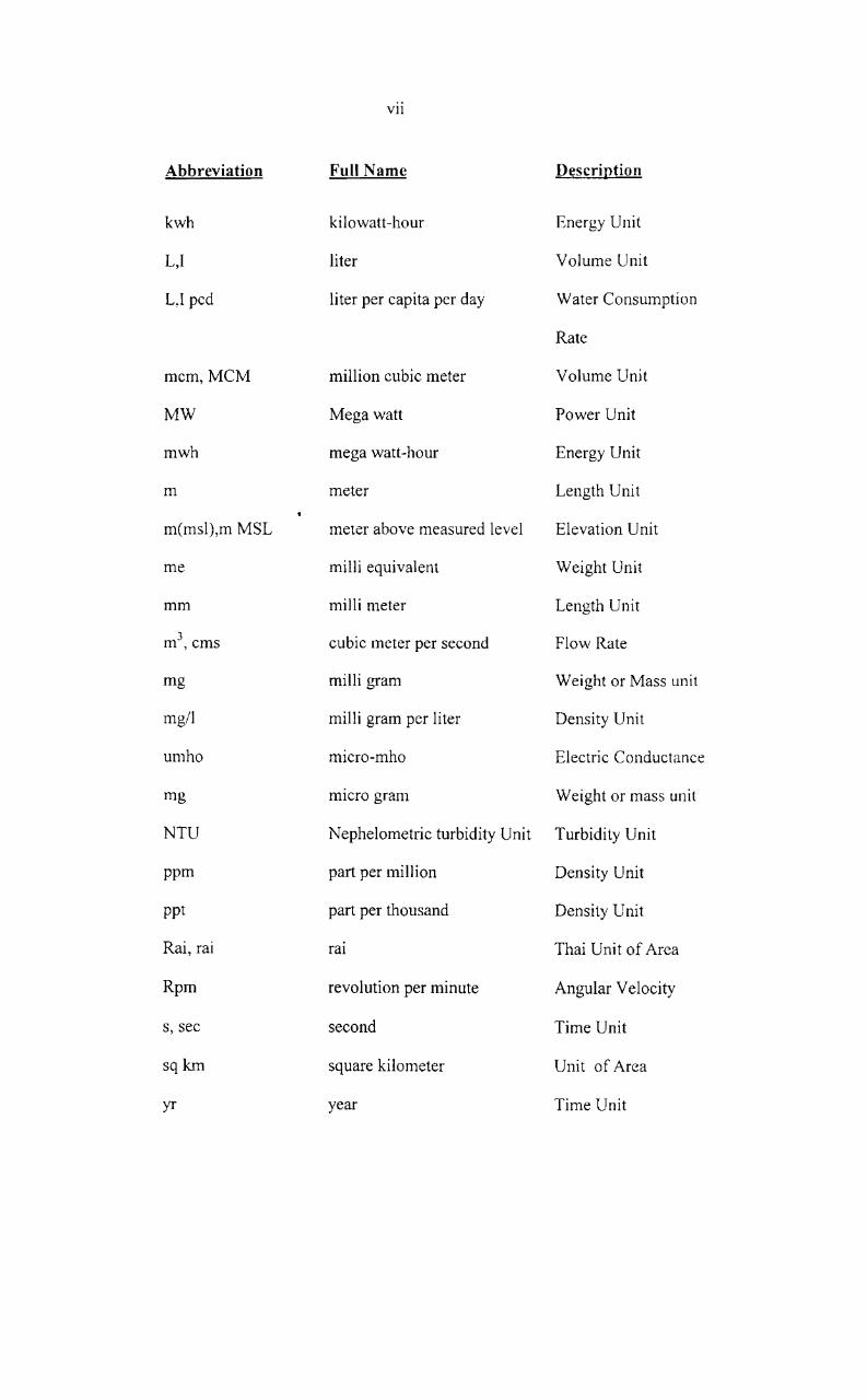
Abbreviation Full Name Description

kwh kilowatt-hour Energy Unit

L,I liter Volume Unit

L,I pcd liter per capita per day Water Consumption

Rate

mem, MCM million cubic meter Volume Unit

MW Mega watt Power Unit

mwh mega watt-hour Energy Unit

m meter Length Unit

m(msl),m MSL meter above measured level Elevation Unit

me milli equivalent Weight Unit

mm milli meter Length Unit

m3, cms cubic meter per second Flow Rate

mg milli gram Weight or Mass unit

mg!l milli gram per liter Density Unit

umho micro-mho Electric Conductance

mg micro gram Weight or mass unit

NTU Nephelometric turbidity Unit Turbidity Unit

ppm part per million Density Unit

ppt part per thousand Density Unit

Rai, rai ral Thai Unit of Area

Rpm revolution per minute Angular Velocity

s, sec second Time Unit

sqkm square kilometer Unit of Area

yr year Time Unit

V III

CONVERSION TABLE

1 inch 2.54 em

] mile 1.6093 km

]km 0.6214 mile

lm 3.28 ft

1 rai = O. ]6 ha

] ft2 0.0929 m2

1 m2 10.7584 ft2

1 hectare 6.25 ra!

] km2 100 hectares

] km2 625 rm

1 rai 1,600 m2

1 ft3 0.0283 m3

1 m3 35.31 ft3

1 mem 10,00,000 m3

1 cfs 0.0283 ems

1 ems 35.31 cfs

1 Mkwh 10,00,000 kwh

1 Gwh 10,00,000 kwh

IMW 1,000.00 kw

1 kg 2.205 pounds

1 ton 1,000 kg

IX

T ABLE OF CONTENTS

Pages

CERTIFICATE

DECLARA TION

ACKNOWLEDGEMENT

GLOSSARY AND ABBREVIATIONS III

T ABLE OF CONTENTS IX

CHAPTER I · THE APPROACH · 1. INTRODUCTION

2. STATEMENT OF THE PROBLEM

3. PROJECT BACKGROUND 2

4. OBJECTIVES 3

5. SCOPE OF THE STUDY 4

6. HYPOTHESES 5

7. METHODOLOGY 6

8. LIMITATIONS OF THE STUDY 20

9. SCHEME OF THE STUDY 21

CHAPTER 11 · REVIEW OF LITERATURE 22 · 1. ENVIRONMENTAL IMP ACT ASSESSMENT (EIA) 22

2. EV ALUATION ENVIRONMENTAL VALUE 31

., ENVIRONMENTAL ECONOMICS EVALUATION 35 -'.

x

Pages

CHAPTER III : PROJECT DESCRIPTION 53

1. INTRODUCTION 53

2. PROJECT LOCATION 53

3. THE PROJECT PURPOSE 55

4. PROJECT FEATURES 55

5. PROJECT DESIGN 63

6. COSTS AND PROGRAMMES 75

CHAPTER IV : PHYSICAL RESOURCES 83

1. INTRODUCTION 83

2. CLIMATE AND SURF ACE WATER HYDROLOGY 83

3. GROUND WATER RESOURCES 93

4. WATER QUALITY 102

5. SOIL AND LAND CAP ABILITY 110

6. MINERAL RESOURCES 119

7. EROSION AND SEDIMENT A TION 124

8. SALINITY INTRUSION 131

CHAPTER V . ECOLOGICAL RESOURCES 135

l. INTRODUCTION 135

2. AQUATIC ECOLOGY AND AQUATIC WEED 135

3. FISHERIES 147

4. FORESTRY 167

5. WILDLIFE 193

Xl

Pages

CHAPTER VI . HUMAN USE VALUES 198 .

l. INTRODUCTION 198

2. LAND USE 199

3. IRRIGA TION AND WATER SUPPLY 213

4. TRANSPORTATION AND NAVIGATION 231

5. HYDRO POWER PRODUCTION 243

6. FLOOD PROTECTION 254

7. WATER POLLUTION 266

CHAPTER VII : QUALITY OF LIFE VALUES 272

1. INTRODUCTION 272

2. SOCIO-ECONOMIC AND RESETTLEMENT 273

3. PUBLIC HEALTH AND NUTRITION 296

4. TOURISM, RECREATION AND AESTHETICS 307

5. ARCHAEOLOGICAL AND HISTORICAL VALUES 332

CHAPTER VIII ECONOMICS EVALUATION OF ENVIRONMENTAL

CONSEQUENCES 337

1. IMPLICATION ON REGIONAL ECONOMICS 337

2. EVALUATION OF ACTUAL POSITIVE BENEFITS 348

3. INPUT-OUTPUT ANALYSIS 381

Xll

Pages

CHAPTER IX CONCLUSIONS AND RECOMMENDATIONS 400

1. INTRODUCTION 400

2. OBJECTIVES 400

3. HYPOTHESES 401

4. SCOPE OF THE STUDY 401

5. METHODOLOGY 401

6. MAJOR FINDINGS OF THE STUDY 402

REFERENCE 408

Xlll

LIST OF TABLE

No. of Table Title

3.1

4.1

4.2

4.3

4.4

Final project cost estimate.

Statistics of station mean annual rainfall.

Average annual rainfall over reservoir and river basin.

A verage annual monthly evaporation at damsite.

Annual stream flow pre and post dam in the watershed area.

4.5 The number of the Deep Wells Drilled during 1974-1996 in the

watershed Area.

4.6 Utilization of Deep Wells Drilled.

4.7 Comparison of ground water levels in the watershed area after with

those observed in the previous investigation

4.8 Physical-Chemical properties of water samples taken from reservoir,

and the Phum Duang river on pre-impoundmentation period.

4.9 Water quality in the reservoir and Phum Duang rive

post-implementation preiod.

4.10

4.11

4.12

4.13

4.14

4.15

4.16

4.17

Land capability cclassification in upstream area.

Land classification in Phase I irrigation project area.

Previous mining concession in the watershed area.

Existing mining concessions in the watershed area.

Mine production in the watershed area (January-April 1996).

Annual depths of erosion in various watershed.

Erosion and Sedimentation of EGA T ' s dam.

Channel improvement in Ao Ban Don estuary by dredging.

Pages

81

88

89

90

92

96

98

99

106

108

113

116

121

122

123

126

128

130

XIV

No. of Table Title

5.1 Standing crops of fish population in previous investigation

(December 1980).

5.2 Standing crops of fish in Rajjaprabha reservoir and downstream area.

5.3 Comparison of fish population during pre and post impoundment

periods.

5.4 General information of sample households in reservoir and

downstream area.

5.5 General information on fish occupation of household in

upstream and downstream area.

5.6 Production of some fish species cultured in ponds in Surat Thani.

5.7 Favourite species of fish raised in ponds in Surat Thani, 1997.

5.8 Forest types in the reservoir before impoundmentation.

5.9 Summary of net profit of all types of timber in reservoir.

5.10 Forestry types in Phum Duang river basin.

5.11 Forecast of future forest area in the catchment area.

5.12 Total present and future value of net income from uncut forests

manage on sustained yield basis.

5.13 Wild animal in the river basin pre-and-post impoundment.

6.1 Land use in the reservoir area before proj ect impoundment.

6.2 Land use in irrigation area, as of 1980.

6.3 Present land use in the Phum Duang river basin.

6.4 Comparison of land use in the upstream area before and after the

dam implementation.

6.5 Change of land use in the Phase I irrigation area before and after

the dam implementation.

Pages

152

154

155

157

158

165

166

17l

172

174

185

192

197

201

202

205

207

208

xv

No. of Table Title

6.6

6.7

Economic analysis of Para-rubber plantation.

Economic analysis of agricultural potential in the reservoir area.

6.8 Project population in Surat Thani province and in Phum Duang

rural zone.

6.9 Water consumption in Surat Thani Municipality, Phun Phin district

and Phum Duang rural zone.

6.10

6.11

6.12

6.13

6.14

6.15

6.16

6.17

6.18

6.19

6.20

6.21

6.22

6.23

6.24

7.1

7.2

Projection of future water demand (1995-2010).

Average percentage of traffic composition on 15,16 May 1997.

Average daily traffic from the Highway Department recorded.

A verage daily traffic from field investigation.

Volume capacity ratios.

Number of boats counted at Surat Thani during 2 hours period.

Benefit flow of Rajjaprabha dam.

Cost flow of Rajjaprabha dam.

Finance benefit to EGAT.

Finance benefit to PEA.

Previous flooded in Surat Thani province.

Estimation of flood damage separated into district.

Estimation of domestic BOD loading to the Phum Duang river.

Estimation BOD loading from industrial waste and fish landing pier.

Estimation of BOO loading from irrigation return flow.

General characteristics of farmer in the study area.

House and other facilities of the farmers in the study area.

Pages

210

211

225

228

229

234

235

236

238

241

249

250

252

253

256

259

269

270

270

275

276

XVl

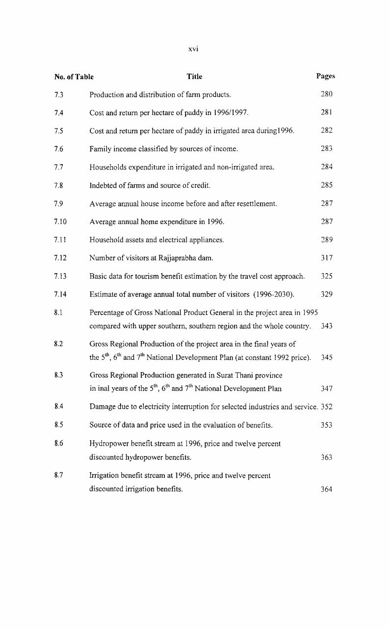
No. of Table Title Pages

7.3 Production and· distribution of farm products. 280

7.4 Cost and return per hectare of paddy in 1996/1997. 281

7.5 Cost and return per hectare of paddy in irrigated area during1996. 282

7.6 Family income classified by sources of income. 283

7.7 Households expenditure in irrigated and non-irrigated area. 284

7.8 Indebted of farms and source of credit. 285

7.9 A verage annual house income before and after resettlement. 287

7.10 A verage annual home expenditure in 1996. 287

7.11 Household assets and electrical appliances. 289

7.12 Number of visitors at Rajjaprabha dam. 317

7.13 Basic data for tourism benefit estimation by the travel cost approach. 325

7.14 Estimate of average annual total number of visitors (1996-2030). 329

8.1 Percentage of Gross National Product General in the project area in 1995

compared with upper southern, southern region and the whole country. 343

8.2 Gross Regional Production of the project area in the final years of

the 5th, 6th and t h National Development Plan (at constant 1992 price). 345

8.3 Gross Regional Production generated in Surat Thani province

in inal years of the 5t\ 6th and t h National Development Plan 347

8.4 Damage due to electricity interruption for selected industries and service. 352

8.5 Source of data and price used in the evaluation of benefits.

8.6 Hydropower benefit stream at 1996, price and twelve percent

discounted hydropower benefits.

8.7 Irrigation benefit stream at 1996, price and twelve percent

discounted irrigation benefits.

353

363

364

XVll

No. of Table Title

8.8 Water supply benefit stream at 1996, 1987 price and twelve percent

discounted water supply benefits.

8.9 Flood protection benefit stream at 1996, 1987 price and twelve percent

discounted flood protection benefits.

8.10 Fisheries benefit stream at 1996, 1987price and twelve percent

8.11

8.12

8.13

8.14

8.15

8.16

8.17

8.18

8.19

8.20

discounted fisheries benefits.

Estimate traffic volume and benefit stream at 1987 price and twelve

percent discounted transportation benefits.

Forestry benefit stream at 1987 price and twelve percent

discounted forestry benefits.

Tourism benefit stream at 1987, 1996 price and twelve Percent

discounted tourism benefits.

Estimation of population during 1987-2037.

Benefit from decrease of health care.

Benefit from increased earning in cost of person.

Health improvement benefit stream at 1996, 1987 price and twelve

percent discounted health improvement benefits.

Resettlement benefit stream at 1996, 1987 price and twelve percent

discounted resettlement benefits.

Comparison of benefits estimated before and after project

implementation.

Technical Coefficients for regional economy.

8.21 Total effects in the economy due to an exogenous change in final

demand.

Pages

365

366

367

368

369

370

371

372

373

374

375

378

384

388

XVlll

No. of Table Title Pages

8.22 Total production and income effects in the economy due to an

exogenous change in other demand. 390

8.23 Total effects generated on production, import, pollution and income

of the economy, with and without income consumption linkages. 392

8.24

8.25

Direct and indirect impact on output and income of existing benefits.

Direct and indirect impact on output and income of full benefits.

398

399

XIX

LIST OF FIGURES

No. of Figure Title Pages

3.1 Location Map of Rajjaprabha project. 54

4.1 Phum Duang river basin and climatic sampling stations. 86

4.2 Monthly climatic statistics at selected stations surrounding

the Phum Duang river basin region. 91

4.3 Water quality sampling stations. 104

5.1 Plankton and fish sampling stations. 151

6.1 Irrigation area. 216

6.1 Road net work in Surat Thani province. 239

6.2 Present and future powers supply system. 246

6.3 Zone of flood area subjected to exceptional flood event

Phum Duang river basin. 260

6.4 Flood damage frequency curves of Khirirattha Nikhom

and Ban Ta Khun district in combination. 263

6.5 Flood damage frequency curves of Phun Phin district. 264

7.1 Sub-basin in the Phum Duang river basin. 295

7.2 Locations of tourist site in Surat Thani province. 313

7.3 Zones used in travel cost approach. 323

7.4 Recreation demand curve. 328

CHAPTER I

INTRODUCTION

1. INTRODUCTION

CHAPTER I

THE APPROACH

Post Environmental Evaluation (PEE) of a development project falls vv'ithin the

preVIew of applied research. The evaluation is done by taking into consideration the

environmental consequences of the project. Thus it is a systematic examination of the

environmental and socio-economic consequences of the project after its implementation

Environmental evaluation of Rajjaprabha dam is done ill three stagc') \i7., (i)

during the project feasibility study stage (ii) during construction stage and (iii) dUrIng

project operation stage. This study is done in the third stage i.e. the project operation stagc.

2. STA TEMENT OF THE PROBLEM

The socio-economic infrastructures are instrumental in all developmental

efforts and they help in making rural living more comfortable. Creation of infrastructure

facilities opens new vistas for employment, ameliorate economic status and enhance the

living standards of the common people. Therefore the infrastructure establishments in all

area aim to bring about positive changes in welfare and equity. Economic changes lead to

better employment and productivity. The total infrastructure, as such, includes transport,

communication, rural industries, rural electrification and marketing. The developing

countries, which stress industrial development to enhance production for sutlicient

provision of goods, often experience short hlll in energy. Electrical energy is the primary

3

reselVoir with 240 MW hydropower plant located about 90 km upstream from Surat Thalli

province, and irrigation diversion dams with irrigation and drainage systems located in the

coastal plain in Surat Thani province. The upstream storage reservoir has about 5,639 mCIll

storage at its normal high water level. That, hydropower plant had already been

implemented by the Electricity Generating Authority of Thailand (EGA T) during 1980-

1987. The first phase of irrigation system development for irrigating 144,375 rai (23,100

hectares), net paddy area including the diversion dam at Phun Phin district and downstream

flood protection works are presently under construction, with the Royal Irrigation

Department (RID) as the implementing authority. The second phase irrigation system

planned for irrigating about 313,000 rai (50,000 hectares) area with the diversion dam at

Khlong Yan, has not yet been implemented. The benefIcial impacts from the project after

completion includes: (1) generation of power (about 554 kwh per year from the 240 MW

installed capacity plant) (2) irrigation of about 50,000 hectares of paddy land and (3) flood

protection and drainage for the towns of Surat Thani and other downstream communities

(including the paddy areas in the coastal plain). A detailed project description is given In

chapter Ill.

4. OBJECTIVES

The objectives of the study are:

(1) To investigate in detail all existing environmental resources and values

usmg input output analysis. The impacts will be shown at four levels

(Physical resources, Biological resources, Human use values, and Quality

of life values)

(2) To evaluate the beneficial impacts of the project.

4

(3) To compare the actual positive effects with the estimated effects.

(4) To identify the changes vis-a- vis the impacts previously assessed

5. SCOPE OF THE STUDY

The scope of the study is limited to the Phum Duang river basin. Emphasis is

being placed on the areas upstream and downstream of the damsite which arc affected

directly by the project. The environmental impacts are evaluated at four levels viz., (1)

physical resources (2) biological resources (3) human use values and (4) quality of life

values. This is based on the methods proposed by U.S. Corps of Engineers, (Battelle

Pacific Northwest Laboratories, 1974) which has been adopted as a guideline for

environment impact assessment (EIA) preparation by the National Environmental Board

(NEB) of Thailand. This methodology envisages an item-by-item study (case study) of

the following effects:

Level I

Level II

Physical Resources

- Climate and Surface Water Hydrology

- Ground Water Resources

- Surface Water Quality

- Soil and Land Capability

- Mineral Resources

- Erosion and Sedimentation

- Salinity Intrusion

Ecological Resources

- Aquatic Ecology and Aquatic Weeds

5

- Fisheries Resources

- Forestry Resources

- Wildlife Resources

Level III Human Use Values

- Land Use Pattern

- Irrigation and Water Supply

- Flood Protection

- Hydropower Production

- Water Pollution

Level IV Quality of Life Values

- Socio-Economic and Resettlement Aspects

- Public Health and Nutrition Condition

- Tourism, Recreation and Aesthetics

- Archaeological and Historical Values

An overall economic evaluation of the river basin is included in this study.

~ HYPOTHESES

The following hypotheses are formulated for the study.

(l) The adverse effects of the darn are not significant on the physi cal

resources in the project area.

(2) The negative impacts on the ecological resources on the project \vill be

confined to the project area alone.

(3) The Rajjaprabha dam has positive impacts on the economy and the

standard ofliving of the people in the Phum Duang river basin.

7. METHODOLOGY

7.1 Data Collection

Both primary and secondary data were used for the study.

(1) Primal), Data

The pnmary data were collected through tIeld studies. A combinatiol1 of

methods such as:

1. Field reconnaissance through observation to check the land use pattern,

mineral resources, ground water resources, erosion, flood and irrigation,

2. Inventory assessment to check the impact on forestry, \vildlife, fisheries,

and aquatic animals.

3. Took samples for evaluating water quality, water supply, and drinking

water.

4. Traffic counting to evaluate the impact on surface transportation and

navigation.

5. Field survey using a questionnaire to evaluate the impact on the socio­

economic aspects and tourism.

(2) Secondary Data

Secondary data for the study were mainly collected from published sources.

The major sources of secondary data were Thai central government oftlce; (i) the

Electricity Generating Authority of Thailand (ii) the Royal Forestry Department (iii) the

Royal Irrigation Department (iv) the Royal Land Development Department (v) the

Fisheries Department (vi) the Department of Mineral Resources (vii) the Higl1\vay

Department (viii) the Harbor Department (ix) the Department of Meteorology (x) the

Department of Fine Arts (xi) the Tourism Authority of Thailand (xii) the National Energy

Administration (xiii) the Provincial Waterworks Authority (xiv) the Communicable

Diseases Control Department and (xv) the Ministry of Public Health.

Data were also obtained from varIOUS local oHices like; (i) Surat Thani

Provincial Office (ii) a District Office of Ban Ta Khul1 (iii) Surat Thani Provincial Public

Health Office (iv) Ban Ta Khun district Public Health Office (v) Malaria control zone 4

(vi) Surat Thani Provincial Fisheries OfIice (vii) Provincial Highway Oftice (vii) Sural

Thani Region Forestry Office (viii) Provincial Accelerated Rural Development Office (ix)

Provincial Mineral Resources Office (x) Provincial Agricultural Omce (xi) Provincial

Land Office (xii) Provincial Public Welfare Office (xiii) Surat Thani and Phun Phin clistrlct

Waterworks (xiv) Land Development Provincial Office and (xv) Local Royal Irrigation

Department Offices at Phang-Nga.

7.2 Data Analysis

The following tests were used for analyzing the data.

(1) Percentile method: This method is used to present the characteristics of

the environmental and socio-economic aspect in the watershed area.

(2) Chi Square test : This test is employed to determine if similarity or

difference (or neither), in the given parameter during pre and post study (Sidney Siegel

1956). The formula used is:

X2

(df,a)

n L

i=l

k L j=l

(f 0 - f~ )2 I1 I] (l.!)

fe IJ

where

fo 1J

fe 1J

df

a

n

k

Chi-square value

Observed frequency

Expected frequency

k n (L: f)(I f) j=l ij 1=1 1.1

n k L: L f

i=} j=l IJ

Degree of freedom n + k - 1

Level of significanse

Number of characteristic used tcn comparison

Number of groups of samples being compared

(3) Likert method : This method is used to determine attitudes of the people

in the watershed area (Sidney Siegel, 1956) employing the following formula.

-X

Where

N

n I fi Xi

i=1 ( 1.2)

N

Likert's weighted score

Total no. of opinions designated for a given ques\ioll'

i th opinion or attitude expressed when a question is asked

Designated unit weight of the i th opinion

Total number of observation.

n L C

i=1

9

7.3 Evaluation of Environment Values

The three types of economic analysis are employed for the evaluation or

environmental values. They are presented below :

7.3.1 Market Value

The net benefit per unit (NBU) is measured using the Halvorscll and Rubbv

equation (Halvorsen and Ruby, 1981).

i1EV Po i1Qt (lies-I led) [I + (i1Qd 2Qo)] ( 1.3)

where i1EV Value of environment quality changes

es Elasticity of supply

ed Elasticity of demand

Q Number of product

i1Qt QI - Qo

7.3.2 Travel Cost Method (TCM)

The travel cost approach is a way to put monetary value on non-priced goods.

This approach was initially developed to value benefits received by consumers from their

use of an environmental good such as a lake or a darn. The approach imputes the price­

quantity reactions of consumers by examining their travel costs. The main idea behind thIS

method is that the cost of travelling to particular site influences the number of visits made

to it (Bateman, et.al. 1992).

10

The relationship can be expressed as :

where

v

V

TC

7.3.3 Survey Techniques

f(TC, X, ... Xn)

number of visits,

travel cost,

other explanatory variables.

(1 4)

The survey technique is a contingent valuJtion method (CYr\·1). Thi~ study i~

based on an open-ended questionnaire to evaluate the willingness to pay (WTP) and

willingness to accept (WTA), (Direk and Pornpen, 1995).

7.4 Economic Evaluation of Environmental Impacts

The economic evaluation of environmental impacts is conducted at three levels

VIZ., project level, regional level, and the economy of Surat Thani province The last has

been evaluated with the help of input-output analysis.

In order to ascertain the full impact, along with the usual input-output model,

household income-consumption matrices and pollution count are also added.

Considering the project area as a closed system does the economic evaluation

of environmental impacts on the project region. But this approach has limitations: (i) the

benefits and costs that the project generates in the area can be part of a much larger fabric

(ii) the project may involve the movement of people into or out of the project area (iii) the

project area problem can be better understood in the content of a larger ecosystem.

] 1

7.4.1 The Economic Impact of Environmental Consequences

The economiC impact of environmental consequences at the regional le\'eJ 1:'

evaluated by:

(a) Collecting basic data on natural resources at regional/sub-regionallcvcl~

(b) Collecting social and economic data on key regional and sub-regional

variables

Cc) Studying the relationship between region and project area;

(d) Defining preliminary regional/sub-regional strategies; and

( e) Assessing implication on regional economics of the proj ec!

The impacts are simply determined by the difference between the condition::;

with and without the dam, To avoid the difficulty in calculation, the impact calculation \vill

begin with the net irrigated areas receiving water from the dam and proceed to determine

the impacts on different aspects by the following formulas:

(1) The impacts on production

(1.1) Production change In provmce IS evaluated usmg the follmving

where

formula:

s Y itj

L: (ysiti t=1

n

A R it.! - Y itj

Change in quantity of commodity in province j

( 1,5)

Yield of commodity i in the irrigated area under the

project at time t in the province j

13

n L eVilJ - C;j )

T=1 (I 9)

where Change 111 ITlcome resulted from producing

commodity

Production value or commodity at time t in the

provll1ce J

Production cost of commodity i at the province j

(3.2) Change in income of the whole project is calculated as follows;

I

where

n m s L L I (Vilj - C;j ) i=1 t=1 j= 1

Change in total income due to the project.

(4) Impacts on cropping patterns and systems

(I. 10)

The impacts on the croppmg pattern can not be exactly quantified. The,,',

however, can be simply determined by the comparison of crops planted in the wet and dry

seasons at the period before and after the construction of the dam. On the other hand

impacts on the cropping systems are determined by the differences in areas of rice and

other crops planted in year-round. The impacts can quantified in total production value.

7.4.2 Evaluation of Actual Positive Benefits.

The main objectives of this study are the following:

(a) To estimate the demand for electricity and the damages due to electricity

interruption

(b) To evaluate the actual positive benefits after the project implementation and

to compare them with the estimated values before the project construction

14

(c) To identifY all significant changes In benefits from the previollsl~'

estimated ones; and

(d) To assess the multipurpose water resource development as previously

estimated.

To fulfiIl the above objectives, the following methodologies are adopted for

the first objective, data and information were collected from 12 selected industrial and

service units utilizing pre-tested interview schedules. Information \vas collected on number

of workers per industrial unit, labour per hour, value of product produced per hour, cost or

electricity per hour, damages due to electricity interruption per hour, ability to gellcl'illL:

own electricity, and cost of fuel for generating own electricity per hour, Damagc due to

electricity interruption includes two components: direct damages and indirect damages.

Direct damages consist of loss in quantity and quality of products or outputs and storable

inputs during electricity interruption. Indirect damage considered is only the labour cost,

which is the cost of non-storable input.

With respect to the second objective, which consists of benefits from

hydropower, irrigation, water supply, flood control, fisheries development, transportation

and navigation, salinity and water pollution control, tourism, health improvement. and

resettlement were evaluated. The data and information Llsed in the evaluation of these

benefits were obtained from primary and secondary sources, The methods used in

evaluating the various components are as follows:

(a) Benefits from hydropower

cost of having such electricity from the most competitive alternativ:,:

source.

is

Cb) Benefits from irrigation

total net value of crop production with irrigation project - total net value

of crop production without irrigation project.

Cc) Benefits from water supply

cost of next cheaper alternative water source for domestic and industrial

usage.

C d) Benefits from flood protection

saving due to reduction in physical damages in the tlood prone area .,.

saving in expenses which otherwise \vould have to be incurred III

connection with flood control, increase in transportation cost, ere .­

benefit resulting from more efficient and productive uses of the flood

prone area owing to protection + health hazard cost reduction r securtty

and loss of life prevention.

( e) Benefits from fisheries development

increase in value of reservoir fisheries - (value of downstream loss

during the construction + value of downstream [ass after impoundment

+ value of loss of migratory species) + benefit of aquaculture USlllg

water supply from the project.

(t) Benefits from transportation and navigation

(cost of using road transportation instead of reservoir and downstream

navigation - cost of using reservoir and downstream navigation) - (cost

of relocation for transportation instead of reservoir and downstream

navigation + maintenance cost for relocated roads).

16

(g) Benefits from salinity and water pollu:ion control

(total net value of crop production with salinity intrusion control·· total

net value of crop production without salinity intrusion control)

(h) Benefits from forestry

benefits from decreases III deforestation and illegal logging - value of

loss of forest products in reservOIr area - value of loss of wood tl-om

trees in reservoir area.

(i) Benefits from tourism

revenue received from visitors who come for the purpose of recreation -;­

revenue received from visitors who come for other purposes -;- revenue

from expenditure of visitors.

(j) Benefits from health improvement

increase in earnings of person resulting from improvement of health +

decrease in the cost of health care resulting from improvement of health

owing to the project; and

(k) Benefits from resettlement

= Post resettled household income - pre-resettled household income

The pre-post evaluation form was used to compare the actual positive benefits

after construction of the dam with the pre-project evaluation of the benefits from the

project outputs (evaluated after the implementation of the dam).

By this method, all significant changes in benefits from the project after its

implementation from the previously estimated benefits can be identified, this fulfils the

third objective. Thus, the last objective involving assessment of the multipurpose water

resource development as previously estimated can be achieved.

7.4.3 Input-Output Analysis

The main objective of this study is to analyze the direct and indirect effects of

Rajjaprabha dam on output, income and environment in Surat Thani. Therefore, the

administrative boundary of Surat Thani province is defined as a region specific economic

system. Production sectors within the area are treated as "domestic" production sectors al1ci

those outside are aggregated as "the rest of the world". [nflmv of goods and services hum

the rest of the world are considered as "imports" while outflmv of goods and services from

the region, "exports".

Methodolo2Y

(1) Model: In addition to the usual input-output matrix, household incoll1c­

consumption matrices and pollution row are included in the modeL The model is described

as follows:

Material balance equation

x AX+BY+F (l.1 I)

Income equation

y YX+T ( 112)

Imports equation

M CX+DY (113 )

Pollution equation

Q PX+ SY ( 1 . I-f)

Where X

A

B

F

V

T

M

C

D

Q =

p

S

In matrix form

I-A -B 0 o

o

o

I

-V I 0

-C -0 I

-p -S 0

X

Y

M

Q

I-A -B 0

-V I 0

-C -D I

-p -S 0

18

column vector of output (baht).

input - output coeftlcient matrix.

expenditure - income (value added) (baht)

other demands (baht).

value added - output coeftlcient matrix.

other net transfer payment (baht).

total imports (baht).

import-output coeflicient vector.

import-income coeftlcient vector.

total pollution (BOO) in kg.

pollution output coefficient vector.

pollution income coefficient vector.

X

Y

M

Q

o

o

o

I

-1

F

T

o

o

F

T

o

o

19

The first matrix equation (1.8) shows direct structural linkages, while its

inverse in equation (1.9) indicates total (direct and indirect) linkages Except for pollution,

all variables are measured in value terms. Pollution is measured by BOO per bah! of output

produced.

To analyze the impacts of the project, the model is slightly changed. As

indicated before Rajjaprabha dam affects the economy In vanous ways The changes

primarily caused by the dam are regarded as an exogenous change in the system. This

change also generates indirect effects on the economy. The model to derive direct and

indirect effects on the economy due to an exogenous change in supplies of particular

sectors can be formed as follows:

K -B 0 0 -l+A!:: 0 o o o x~ 0l AI-: 0 o o o o :\ I

F I o _Vt'. I 0 0 1: Y

M

Q o

vE 0 o o

o o

o o o

Tr; I

L~J o o

o o

Or J. K + L ( 1I7)

H G- 1 (J. K + L)

where superscript N refers to sectors not primarily affected by the dam.

E refers to sectors primarily affected by the dam.

K = refers to household.

The solution gives sectoral output, household lIlcome, imports and pollution

directly and indirectly generated by the project.

20

(2) Data The 1975 national input-output transaction tablc is used as a basIs

to derive regional technical coefficient matrix. Important production activities arc

identified based on economic profile of the region. Production activities are aggregated

into 36 sectors. Households are differentiated between agricultural and non-agricultural

households. The adapted transaction table is used to derive technical coeHicicnt matrix for

the regional economy. Technical coefficients for households (income and consumptinll)

are derived from the social account matrix for Thailand. Primary data from survey, spot

check and secondary data of various sources are used to cross check the technical

coefficient matrix. Certain cells have been adjusted. Observation in the area suggests that

air pollution is not an important element. Hence, only water pollution is emphasized. As

suggested from water quality studies, few industries have potential to be pollutant

generators. Their pollution coefficients are obtained from water quality study. Each row

represents supply of goods and services from a row sector to various column sectors. Each

column represents demand for goods and services from various row sectors. Row

households refer to value added to households while column households refer to

consumption of households.

8. LIMITATION OF THE STUDY

The study is limited to the 10 years period from the date of completion of the

darn i.e. 1987. It is true that the period of study is not sufficient to appraise the changes

and effects of the darn on physical resources such as climate, geology, land capability, ete

Hence, l:he results emerged from the study are only tentative.

9. SCHEME OF THE STUDY

The thesis is organized under ninth chapters. The first chapter provides the

introduction. It explains the statement of the problem, project background, objectives,

scope and methodology etc.

The second chapter presents a review of literature in the area of study.

Detailed information about the project such as the project location, project

purpose, features, design, etc are provided in the third chapter

The fourth chapter provides information relating to climate, surface \vater

quality, erosion and sedimentation, ground water resources, soil resources, etc.

Biological resources such as fisheries, forestry, wildlife, aquatic ecology,

aquatic weeds are dealt with in the fifth chapter.

The sixth chapter explains human use values that benefit from power

production, flood protection, crop irrigation, drinking water, water supply, land use pattern,

water pollution etc.

The seventh chapter deals with quality of life values; socio-economic and

resettlement aspects, public health and nutrition conditions, tourism, recreation and

aesthetics, archaeological, and historical values.

The eighth chapter presents the economIc analysis of environmental

consequences assessment.

The ninth chapter presents the summary and conclusion

CHAPTER 11

REVIEW OF LITERA TURE

CHAPTER II

REVIE"V OF LITERATURE

1. ENVIRONMENTAL IMPACT ASSESSMENT (EIA)

The guidelines prepared by the National Environmental Board (NEB) of

Thailand for Environmental Impact Assessment (EIA) suggests four levels of

environmental impact assessment viz., (1) physical resources (ii) biological or ecological

resources (iii) human use values and (iv) quality of lift values. (NEB.1979). On the other

hand, Andrew, divides the environmental impact assessment method into seven categories

(Andrew R.N.L. 1973) viz; (1) ad hoc methods (2) checklists (3) matrices (4) overlays (5)

networks (6) Quantitative or index methods and (7) models.

Brief descriptions of these categories with examples are given below.

1.1 Ad Hoc methods

This is the most common approach to impact assessment. Basically ad hoc

methods indicate broad areas of likely impact by listing composite environmental

parameters (for example, flora and fauna) likely to be affected by development activities.

1.2 Checklists

Checklists are an expansion on ad hoc methods in that they list environmental,

social and economic components in more detail. Also, some checklists identif): typical

impacts resulting from certain types of development. Checklists serve as a guide for

identification and consideration of a wide range of impacts.

23

The Multiagency Task Force, (1972) has mentioned that it has also provided a

checklist for evaluating environmental impacts. It suggests that the impacts be expressed

quantitatively whenever possible. Further for each impact the uniqueness of the affected

component and the irreversibility of the expected changes should be considered \vhere

appropriate. It is the predicted future state of the environment, and not the prcscnt

condition, which should be compared with the project proceeds. But it may be seen that the

scope of the checklist is rather limited interms of the features to be investigated. For

example, when cultural resources such as archeological sites are included, social and

economic factors are neglected. However, the explicit consideration of uniqueness and

irreversibility distinguishes this method from many others. This forces those who prepare

the impact statement to consider the post development situation.

Adkin and Burke have provided a checklist for evaluating the environmental

impacts (Adkin.W.G. and Burke D.1974). The components in the checklist are broken

down into four categories VIZ., (i) transport (ii) environmental (iii) social and (iv)

economIc. Impacts on these components are evaluated on a -5 to +5 rating system. This

method is an early attempt to systematize assessment of route alternatives but it suffers

from a number of limitations. The coverage of ecological effects is deficient. Also, the

rating of impacts and alternative routes require subjective judgement, and there are 110

guidelines to aid formulation of these judgements.

1.3 Matrices

In matrices used for evaluating environmental impact usually one dimension of

the matrix provides a list of environmental, social and economic factors likely to be

affected by a proposal. The other dimension provides a list of actions associated with

24

development. These actions relate to both the construction and operational phases There

are many variations to the matrix approach. The best known interaction matrix method was

developed by Leopard and has been used more often than any other method in the

preparation of EIS in the United States.

Leopold's method, (Leopold, et a1. 1971), as mentioned above, is one of the

best known and most widely used methods for EIS. It has been adapted in Cl number of

ways for use in particular impact analyses. The method advocated is really an interaction

matrix in which the existing characteristics of the environment (for exampl~, endangered

species) are listed vertically and proposed project action (for example blasting and drilling)

are listed horizontally. 8800 interactions are identified in the matrix. However, preliminary

trials indicate that specific projects will result in only 25-50 interactions. For each

interaction a score of 1 (least magnitude or importance) to 10 (greatest magnitude or

importance) should be given. It suggests that the cells indicating an impact are slashed and

the scores for magnitude are placed at the bottom right hand section. A+ (plus) sign in the

appropriate cell can denote beneficial impacts. It emphasizes that no two cells in any onc

matrix are equal and that, if separate matrices were prepared for alternative projects, only

the cells indicating the same impact would be comparable. A completed matrix provides Cl

visual representation of an impact statement, as the impact statement should contain a

discussion of the impacts identified. The most important criticism of this method involves

its focus on direct impacts. Second-and higher order impacts cannot be identified easily

Also the matrix does not allow for change in impacts over time.

Welch HW. and Lewis G.O. (1976) assessed environmental impacts of

multiple land use management. "The multi dimensional analysis for the assessment of land

25

use alternative is considered a useful approach as it can show the interactions bel \VCCI1

elements". It also provides a system for identifYing data requirements and the requIred

scientific expertise. A three dimensional matrix is constructed on the basis of the foll()\\'in~

dimensions, viz; analysis of the relationships among various land uses, the institutions

which influence or control these uses, and thc ecological and environmental systcms with

which the uses interact. The effects of a second home development arc used to illustrate its

use, and it can be used to identify whether impacts are of first second, or higher order.

Tofiner R.O. (1973) believes that the impact statement might be a useful

starting point for better environmental planning. However, impact statements often

consider only primary impacts. A matrix, which allows secondary and tertiary impacts, is

necessary to have a complete picture. He considers transport developments to cause the

most far-reaching effects, for example, on land use patterns, land consumption, population

densities expansion of commerce and industry. Through investigations of such secondary

and tertiary impacts, the quality of information available to decision-makers will be

improved. The matrix discussed serves only as a checklist of primary, secondary and

tertiary factors to be considered in an impact statement. Since it is not an interaction matrix

the impact cannot be identified. Also, the category intake checklist is broad, leaving the

detailed break up of these categories for impact identification to those carrying out impact

assessments.

1.4 Overlays

The use of overlay maps has been restricted to route or site selection. Few

examples of their use in environmental impact analysis have been reported. A first, series

of maps, each containing data on environmental, social and economic variables, are

26

prepared. By overlaying the maps, areas possessmg a preferred combination of these

variables can be identified.

Mcharc, also studied the comprehensive highway route selection ll1ethod.

(Mcharc 1. 1968) His paper contains a description of one oC the fIrst methods to be

advocated for impact analysis. The method is based on an overlay of map transparencies,

each map dealing with specific environmental and land-use characteristics. Each or these

characteristics is shaded differently to represent three degrees of "compatibility with the

highway." By using overlayed maps, one of which is the proposed route, a comprehensive

picture showing the spatial distribution and intensity of impacts can be obtained This

composite picture can also be used to select alternative routes by examining areas showing

the greatest compatibility with the highway. This method has served as the basis for a more

sophisticated method developed by Krauskopf and Bund[e. While resource requirements of

the manual overlay method are less demanding than those of computerized versions, thi:,;

method provides less information.

1.5 Networks

Networks are based on known linkages within systems. Thus, actIons

associated with a project can be related to both direct and indirect impacts. For example,

impacts on one environmental factor may affect another environmental or socio-economic

factor and such interactions are identified and listed on a network diagram. This diagram is

subsequently used as a guide to impact identification and the presentation of results. While

there are few examples of the use of networks in impact assessment, the Sorensen net\vork

represents an early attempt to provide a method for tracing impacts using a network

format. For example, Gilliland M.W. and Risser P.G. (1977), used system diagrams for

environmental impact assessment. The usefulness systems analysis and of energy now~

between environmental components as measures of environmental impacts are illustrated

using results obtained from impact statement for the white Sands Missile Range, New

Mexico. The procedure includes five steps: (i) Construction of a systems diagram

representing the important interaction between environmental components and bet\VeCll

man and these component (ii) evaluation of the pathways and storage (iii) analysis of the

data (lv) identification of impacts requiring more detailed attention and Cv) examination of

impacts outside the boundaries of the system. Construction of a systems diagram and

estimation of the impact of human activities on pre-development estimation of energy tlov .. '

between specified environmental components permits a quantitative comparison of the

impacts of alternatives, Hence, actions to mitigate environmental impacts can be easily

made. But it should be noted that a systems approach does not deal with economic, social,

and aesthetic impacts, nor does it guarantee that the boundaries for analysis have been

chosen correctly. Use of this approach requires collection and interpretation of Cl large

amount of data on energy flows between environmental components. In some locations

this data may be difficult to obtain, Consequently, this method IS only useful if

implemented by a large organization having considerable expertise at its command,

Sorensen J. (1971) has attempted to provide a framework for identification and

control of resource degradation and conflict in the case of multiple use of the coastal zones

This structured method allows for identification and control of resource degradation and

conflicts in coastal zones. The framework is based on adverse, environmental impacts that

occurred in the coastal zone of California as a result of a variety of coastal land use. It is

also based upon stepped matrices, occasionally referred to as a network, listing a number

of land uses (for example residential development and crop farming). Factors associated

28

with these land uses (for example, fencing) are related to initial condition changes These,

in turn, are linked to consequent condition changes and final eiTects. Further information

may be slotted into the framework (after the column dealing with the effect) For example,

physical actions taken to ameliorate impacts can be listed. Similarly, codes of practice or

regulations, which may be required to control the effects of a particular land use, can he

inserted into the framework. The framework acts as a checklist to possible adver~e

environmental impacts. Thus, it can be used to identify and control conflicts between

different land uses. The compatibility of a particular land use with an existing land use can

be identified by investigating its likely adverse impacts using the stepped matrix

framework This approach to impact identification is one of the best known attempts to

make the identification of indirect impacts explicit.

1.6 Quantitative on Index Methods

These methods are based on a list of factors thought to be relevant to a

particular proposal and are differentially weighted for importance. Likely impacts are

identified and assessed. Impact results are transformed into a common me(lsurement unIt

(for example, a score on a scale of environmental quality). The score and the factor

weighting are multiplied and the resulting score is added to provide an aggregate impact

score. By this means, beneficial cmd harmful impacts can be summed up, and the total

score can be compared. Additionally all impact scores for two alternative sites can be

aggregated and compared. The alternative resulting in the "best" score will be the preferred

option.

Dee N., et al (1973), have developed a method for assessing the impacts of

water quality management projects. It is based on a checklist of environmental parameters

29

divided into 19 components and a matrix to identify the likely impacts. Impact

measurement incorporates two elements. First, a set of ranges IS specified for each

parameter to express impact magnitude on a scale of 0 to 1. The use of an "environmental

assessment tree" is advocated to combine the parameter scores into a summaly score i'or

each of the 19 components. Second, a set of weights is used to determine the signilicance

of the impacts on each component. A total score for each alternative can be obtained by

multiplying each component score by its weight and summing all the components. The

method, especially the assessment trees, has been developed for water resource projects.

New environmental checklists and assessment tree would have to be constructed for other

types of projects.

Stover L.v. (1972), developed a method for EIA. The most distinctive feature

of this method is the approach for aggregating impacts. Environmental impacts are

assessed for 50 environmental functions. These functions are grouped into the following

categories: ecological and geophysical features, land use, chemical entities, biological

communities, and human well being. Separate estimates are made for short-term and long­

term impacts of each of the 50 environmental functions. Impacts are classified subjectively

into five classes; 1 extremely beneficial, 2 very beneficial, 3 no effect, 4 detrimentaL and 5

very detrimental. Very detrimental formations are given a numerical score of -5 Oil the

scale while an extremely beneficial impact is given a score of +5. The score is multiplied

by the number of years over which the short-term impact is likely to occur. Long-term

impacts are scored on a scale + 10 to -10, where + 10 stands for extremely beneficial and -

10 for extremely detrimental. The aggregate score for environmental impact can be

compared with alternative developments or with the situation in which there is no

development.

30

1.7 Models

Recently, considerable attention has been focused on the use of systems

modeling in impact analysis. However, the development of models for assessing particular

projects is at an early stage. There are few examples of models utilized for the assessment

of the wide variety of impacts resulting from major projects. Usually, only a pal1icular

impact of great significance or a number of key impacts are modeled (for example, the

effects of a nuclear power station on a salmon population). It may require more time before

a modeling approach can cope with the wide diversity of impacts. Modeling is being used

in the development and assessment of alternative strategies for resource management (but

again the models only deal with a few key issues). In the future the use of models in large­

scale resource management problems may become common. However, considerable work

on assessing the impacts of resource management strategies by models has been carried out

at the Institute of Resource Ecology, University of British Columbia by Yorquc ami

Hailing.

31

2. EVALUATION ENVIRONMENTAL VALUE

There are four major categories of direct valuation techniques. These arc (i) thc

use of market prices to evaluate benefits and costs arising ti-om changes in environlllental

quality (ii) the hedonic pricing approach which decomposes market prices into components

of environmental and other characteristics (iii) the contingent valuation approach which is

a. non-market techniques using survey to ascertain peoples willingness to pay for

environmental aesthetics and (iv) the travel cost approach which is a market based

technique that uses travel costs as a surrogate for the price of non-priced recreational and

other amenities. Each of these approaches has its advantages and disadvantages, both [1·0111

a theoretical standpoint and from the standpoint of empirical applicability (Jonathan :\

Lesser, et. al. 1996).

2.1 The Use of Mari{et Prices

The first and easiest valuation technique is to estimate environmental costs and

benefits from market prices. We cannot measure the value of a lost view simply by

walking in to the local shopping mall and inquiring about the price of views. By contrast,

it may be possible to place a value on the damage caused to crops by pollution because one

can easily determine the market price of crop goods.

A standard result in microeconomics is that if a good is sold in a competiti'v'c

market and there are no externalities or underemployed resources, the market price will be

equal to both the marginal buyer's willingness to pay and the opportunity cost of supplying

that good. For example, suppose that pollution reduces wheat yields by only 1 bushel whell

the same supply of land, labour, equipment, fertilizer, water and other inputs is used. The

total production of wheat is measured in millions of tons. Thus, the loss of 1 bllshel of

wheat can be considered a very small change in supply The value of the lost production i~

equal to the market price of that one-bushel of wheat.

2.2 The Hedonic Pricing Approach

The hedonic pricing approach (HP A) is based on a straightfonvard premise that

the value of an asset, whether a piece of land, a car, or a house, depends on the stream of

benefits that are derived from that asset. These include the beneflts of environmental

amenities. One of the most common applications of the HP A has been comparing the

values of real estate with different environmental amenities to estimate the value of those

amenities. Houses have different views or are located in areas with better schools or [oweI'

crime rates. House may also differ in their exposure to pollution. By using regression

techniques, an HP A model can, in theory, identify what pOIiion of the property value

differences can be attributed solely to environmental differences. From this, \ve can infer

individuals willingness to pay (WTP) for environmental amenities and, therefore, the

overall social value of a given amenity. The HJl A can also be used to estimate WTP lo

avoid disamenities.

In the case of environmental externalities, the HP A is often applied la

environmental attributes associated with specific commodities. An HP A model may not be

applicable to certain environmental externalities if those externalities cannot be

decomposed or differentiated within existing market prices. One example is housing prices

and atmospheric carbon dioxide levels. Because carbon dioxide emissions are a global

issue, one should expect housing price to differ depending on local emissions of carbon

dioxide.

33

2.3 The Contingent Valuation Method

The premIse of the contingent valuation methodology (CV1\11) is straight

forward, if one wishes to know the value of something (for example view, clean air, saCcty,

etc) just ask the people. CYM asks people what they are willing to pay for an

environmental benefit or to what extent they are willing to tolerate an environmental cost.

Inquiries may be done through the use of direct questionnaires or surveys or through the

use of experiments that determine how individuals respond. The biggest potential

advantage of CYM is that it is applicable to all situations. Whereas a hedonic study might

be unable to distinguish between the effects of different pollutants, a CYM could ask

individuals about specific pollutants and the desired environmental change directly CV\'1

also ask people about choices that they may not actually make in real life, such as making

direct payments for cleaner air.

2.4 Travel Cost Methods

The fourth technique used to estimate the value of environmental amenities is

the travel cost method (TCM), This method is often used to estimate the value of public

recreation sites, which usually have a zero or nominal admission price. The travel cost

method is based on three observations. First, the cost of using a recreation site is more than

that of the admission price. It includes the monetary and time costs of travelling to the site

and may include other costs, Second, people who live at various distances from a

recreation site face different costs for using the site. Third, if the value that people place on

a site does not vary systematically with distance, travel cost can be used as a proxy for

price in order to derive a demand curve for the recreation site.

34

One can develop the theory behind travel cost models by examining the

relationship 'between distances from a recreation site and number of visits by a single

individual. Suppose one wants to know the value that individuals place on trips to a

pristine beach that lies within the national park of the cost of Maine. An individual taking a

day trip to this beach will incur several costs. The monetary costs of the trip will include

gasoline, wear-and-tear, and the admission price to the park. A less obvious type of cost is

the opportunity cost of time. Time spent at the beach and travelling to and from the beach

could have been spent in other ways. It could have been spent in other leisure activities, it

could have been spent studying or writing, it could have been spent working. The value of

the time used for the trip toward its next best use is the opportunity cost of time for

spending the day at the beach. In many cases, it will be the largest component aftatal cost.

35

3. ENVIRONMENTAL ECONOMICS EVALUATION

The methodologies and techniques for evaluating environmental consequences

were explained by K.c. Sankaranarayanan and V Karunakaran (1984). These are

mentioned below.

1. Cost - Benefit Analysis (CBA)

2. Input - output Analysis

3. Multiple - Objective analysis (MOA)

4. Cost - Effectiveness Analysis (CEA)

5. Risk Benefit Analysis (REA)

6. System Analysis and Optimization Models (SAOM)

7. Trade and Investment Models (TIM)

A brief description of the main characteristics of each type is given below.

3.1 Cost-Benefit Analysis (CBA)

Techniques of Cost-Benefit Analysis for evaluating development projects are

not very old. (Nail K. Shatter 1991) These were used for the first time in 1930 in tbe LIS..\.

for the implementation of water project planning programs. Since then these have been

applied to a wider spectrum of projects, though the emphasis has been on schemcs

requiring a substantial amount of public investments like motor ways, airports, etc. In early

years, these techniques have been widely used to evaluate projects whose outputs were

designed to increase or improve a product. The classic example being irrigation projects

designed to stimulate farm productivity. However, these tcchniques have limitations as

they could suggest evaluation purely in monetary terms. In order to provide a holistic

36

approach for the project appraisal, an alternative technique termed as EIA has been

deployed in the USA since 1970. Since then, EIA has superceded CBA as the principal

advisory tool for decision-makers, but still there are many reasons to regard them as

complementary.

3.1.1 Cost-Benefit Analysis Dimensions

Public investment commitment is a socio-ethical aspects, which is considereel

by planners, as well as policy makers in order to consider the economic viability of

projects. Three important dimensions of CBA have been suggested as an important set of

economic techniques.

POLICIES

COST BENEFIT

ANALYSIS

PROJECTS

PROGRAMMES

(a) Projects are concerned with major resource development schemes, such as

water supply reservoirs or electricity generating stations.

(b) Course of action is related to categorical and systematic programmIng,

such as commitment to a major electric power programme, as part of an

overall energy strategy.

37

(c) Policies, comprised of a definite programs to achieve socio-economic

growth, for example, determination to make energy production self­

financing and hence proposing removal of all subsidies from energy costs.

Thus, the attempt of CBA procedure is to measure and compare all

relevant gains (social benefits) and losses (social opportunity costs) which

would result from a given project.

3.1.2 The Basic eBA Procedure

We can divide the basic CBA procedure in four steps:

(a) identification and listing of all the relevant social costs and benefits

(project impacts) connected with the project or projects.

Cb) collection of the data necessary to quantity the relevant costs and benetits

(c) evaluation (in monetary terms) of the costs and benefits identified by the

analysis.

(d) submission of the finished CBA report and results to the policy makers.

3.1.3 Economic Efficiency: An Important Factor

Consideration of economIc efficiency enables any policy making and

administrative machinery to judge project desirability, as well as to distinguish relevant

costs and benefits. Economic efficiency is said to increase when a reallocation of resources

(such as, building of a dam) stimulates an increase in the net value of social output and its

associated social consumption. The latter would include, among others, the aesthetic and

recreational benefits and also the life support benefits of the environment. The total social

38

costs of a given project must include all the private resource costs and that so called

external costs, which are imposed on people who are only indirectly concerned.

In any given project, the total social benefits should include all the direct, as

well as indirect gains to users of its output. Dams are constructed primarily for irrigation

benefits. They also yield secondary benefits and generate costs, which usually involve

changes in some people's well being at the expense of other. In other words, they create

redistribution effects and, if the strict efficiency approach to CBA is adhered to such

benefits or costs should not be included in the an:llysis unless there are unemployed

resources available.

3.1.4 Measurement of Cost and Benefits

There are two fundamental ethical postulates In relation to any project

evaluation. First, it is assumed that only individual human beings matter and that the

personal wants of individuals should guide the use of society's resources. Further, it is

conventionally assumed that the preferences of the present generation of individuals should

dominate over the possible preferences of future generations. In this way, the analyst will

be able to determine the effect of a given project on any individual's level of \velfare b~i

understanding the individual's own evaluation of wellbeing. Thus, the individual's

evaluation of any project's benefits is measured in principle, by posing the question, "what

would this beneficiary be willing to pay to acquire the benetlts?" Project costs are valued

by asking project losers what is the minimum sum of money they would require making

them feel justifiably compensated for their losses. Any external costs induced by the

project are valued at the minimum amount required by affected parties to compensate them

39

for the imposition of the cost. Thus, the analyst's guiding principle is to value the welfare

effect of the project on the individuals concerned as they would value it in monetary terms.

The second assumption is related to the ethical postulate that the prevailing

distribution of income in society, whatever it may be, is socially "just" and is, therefore,

taken as given. The assumption is then made that all-individual gains and losses induced

by a project can be valued equally, regardless of the income level of any individual

concerned.

In environmental terms, this can be a velY naIve assumption, as monetarY

wealth tomorrow may not always provide solace for the irredeemable loss of quality of the

landscapes and altered natural habitats caused by decisions made today.

In 1973 Joskov J. described the techniques of cost-benefit analysis. He has

discussed, in detail, the problem of identifYing costs (on whomsoever they fall). He also

provided some advice regarding assigning monetary issues to environmental costs.

Roberts. H.A. and Sievering. H. (I976) provided some preliminary guidelines

for conducting economic impact studies. They also suggested several improvements in the

existing methods of evaluation.

3.2 InputMOutput Analysis (lOA)

The first attempt to extend input-output analysis to environmental problems

was made by the originator of input-output analysis, Leontief, (LeontieC 1970). Input­

output analysis for an entire economy is based on the accounting of the flow of goods and

services in monetary terms at a particular time. Part of this flow is an inter project flow,

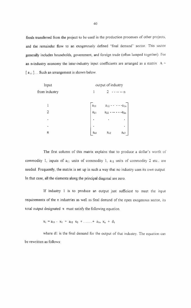
40

foods transferred from the project to be used in the production processes of other projects,

and the remainder flow to an exogenously defined "final demand" sector. This sector

generally includes households, government, and foreign trade (often lumped together). ror

an n-industry economy the inter-industry input coefficients are arranged as a matrix A =

[ajj ). .. Such an arrangement is shown below.

Input

from industry

2

n

output of industry

2 - - -- -- n

The first column of this matrix explains that to produce a dollar's wOlih of

commodity I, inputs of all units of commodity 1, a12 units of commodity 2 etc .. are

needed. Frequently, the matrix is set up in such a way that no industry uses its own output

In that case, all the elements along the principal diagonal are zero.

If industry 1 is to produce an output just sufficient to meet the input

requirements of the n industries as well as final demand of the open exogenous sector, its

total output designated x must satisfy the following equation.

where d 1 is the fInal demand for the output of that industry. The equation can

be rewritten as follows:

41

(*) (1 - all ) Xl - al2 X2 - ... - al n Xn == d)

Except for the first coefficient (l-all), the others are the same as those in rhe

first row of the A matrix (page 52), except they now have negative signs Similarly, if \\ C

write the same type of equation for industry 2, it would have the same coeflicients as in the

second row of A (but with minus signs), except in position a22 where the coefficient \vould

be (l-a22). We can produce this same result in the whole matrix A if we subtract it from the

identity matrix 1. Thus we can write.

(I-A)X = d

where I is an n X n identity matrix, A is the n x n coefficients matrix, and x

and d are both n x 1 vectors, X is the variable vector and d is the final demand vector. If

(I-A) has the rank n (i.e. is non-singular-meaning that the system of equations it represents

has a unique solution), its inverse can be found and the system of n simultaneous equations

represented by the above matrix equation will have the solution.

X = (I - A r) d

Side A provides a solution for the n simultaneous equations, of which equation

(I) is an example, representing commodity and service flow from industries to industries

and the final demand. The inverse matrix (I-A)" I has great utility. Once it is available, this

inverse and a new solution vector produced for the industry outputs X, always on the

assumption that the coefficients of A matrix have not changed, can premultiply d. Since

multiplying a matrix by a vector is a simple operation compared with getting entirely ne\\'

solutions to simultaneous equations, this is a great advantage.

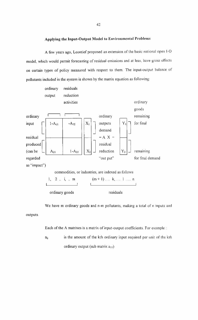
42

Applying the Input-Output Model to Environmental Problems

A few years ago, Leontief proposed an extension of the basic national open 1-0

model, which would permit forecasting of residual emissions and at leas, have gross effects

on certain types of policy measured with respect to them. The input-output balance of

pollutants included in the system is shown by the matrix equation as following:

ordinary residuals

output reduction

activities ordinary

goods

ordinary ordinary remall1ll1g

input [ I-All -A12 Xl ] outputs Yl ] for final

demand

residual =A X =

proctucect[ (can be A21 1-A22

] residual ] X2 reduction Y2 remal!lIllg

regarded "out put" for final demand

as "impact")

commodities, or industries, are indexed as follows

1, 2 .. i, .. m (m + 1) .... k, .... 1 ..... n

ordinary goods residuals

We have m ordinary goods and n-m pollutants, making a total of n inputs and

outputs.

Each of the A matrixes is a matrix of input-output coenicients. For example:

aij is the amount of the kth ordinary input required per unit of the kth

ordinary output (sub matrix all)

43

aik is the amount of the ith ordinary input required to produce a unit

the kth residuals reduction output (sub-matrix a12)

d ji is the amount of the jth residual resulting from producing a unit

the ith ordinary output (sub-matrix a21)

aki is the amount of the kth residual produced as a result of a unit

reduction in the ith residual (sub-matrix a22)

To see what is involved in this system of equations, assume that we have three

ordinary commodities as two pollutant equation activities, making a total of five outputs,

or "inputs", in all. Take, for example, the first equation which is formed by multiplying

each member of the first row of A * by the corresponding members of the X vector of

industry outputs. Add these products together, thereby obtaining the first I1lclllbcL Y I or

the vector or final outputs, Y :

or,

- al2 - al3 - al4 - al5 Xl

X2

X3

X4

Xs

Note that in the matrices of input-output coetJicients aij and aid;, are regarded as

zero so that industry output is always net of its one output that it uses itself.

This equation simply says that the total output of the first commodity minus the

amount used in the production of X2 X3 X4 and Xs is equal to the amount of the first

44

commodity, Y 1 going to final demanders. The last four terms account for all of the XI used

in production, whether for ordinary goods or residual reduction.

Now consider an equation in the bottom part of the square matrix, A *, say the

last one for the nth commodity, which is a residual. Note that since the output of the

residuals processing industry here is measured as residual reduction, the Sign of the

elements in the two lower quadrants are reversed from those in the two upper:

a52 aS3

or,

-I aS4

Ys

aSl Xl + a52 X2 + aS3 X3 + a54 X4 - Xs = Y S

This says that the residual which is commodity number five. That is generated

in the production of XI, X2, X3 and X4 minus the amount by which this residual is reduced

equals the amount which goes to final demanders.

Thus, in abbreviated matrix form, the input-output balance is ;\ * X = Y, \vhere

X and Y are vectors on industry outputs and deliveries of final goods, respectively

Industry outputs include residual reduction, and final goods include residuals rece.ived.

The system of equations, A * X == Y, can be solved for the vector X, industry

outputs, by pre-multiplying each side by the inverse of the matrix, A * -1 Y Thus, if A * -I

has been calculated for a given industrial structure the industry output X would be

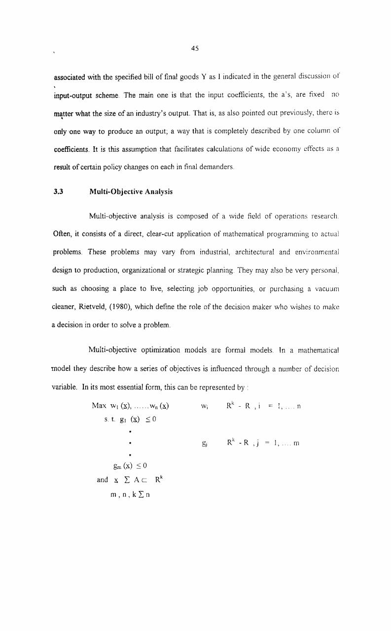
45

associated with the specified bill of final goods Y as I indicated in the general discussion of

input-output scheme. The main one is that the input coet1icients, the a's, are fixed no

matter what the size of an industry's output. That is, as also pointed out previously, there is •

only one way to produce an output; a way that is completely described by one column or

coefficients. It is this assumption that facilitates calculations of wide economy effects as Cl

result of certain policy changes on each in final demanders.

3.3 Multi-Objective Analysis

Multi-objective analysis is composed of a wide field of operations research.

Often, it consists of a direct, clear-cut application of mathematical programming to actual

problems. These problems may vary from industrial, architectural and environmental

design to production, organizational or strategic planning, They may also be very personal,

such as choosing a place to live, selecting job opportunities, or purchasing a vacuum

cleaner, Rietveld, (1980), which define the role of the decision maker who wishes to make

a decision in order to solve a problem,

Multi-objective optimization models are formal models. In a mathematical

model they describe how a series of objectives is influenced through a number of decision

variable, In its most essential form, this can be represented by :

Max Wl (x), , ..... Wn (x)

s. 1. gl (x) S 0

gm (x) SO

and x I: A C Rk

m,n,kI:n

Wi Rk - R , I ;:::: I, .... n

I, ... m

46

where x is the vector of decision variables, gj (x) are constraints on x. W, (.~)

'are objective functions, determined by x. A unique optimum for x is generally not found.

This is where multi-objective optimization methods come in. These methods allow for the

calculation of an optimum or a set of optimal solutions, all depending on when and how

the decision maker assign priorities to the various objectives.

Multi-objective modeling encompasses an enormous variety of techniques,

mathematical representations, computational procedures, etc. Here, \\:e shall treat the

characteristics of multi-obj ective models while distinguishing between the.

a. Decision space, in which a decision is made under varying circumstances;

b. Objective spaces, in which results of the decision are measured;

c. Preference structures, which contains an ordaining in objective space:

d. Optimization procedure, which describes a procedure for finding a set of

optimal solution.

Keeney and Raiffa (1976), use the term "Objective" to indicate the direction of

improvement on a certain aspect of decision-making. They use the term "attribute" to

denote the dimension in which an objective is measured.

From the basics of multi objective analysis, we could make a distinction

between choice processes with a limited number of alternatives and choice processes \vith

a continuous set of alternative. The latter category applies to the choice problem that exists

when economic, employment and environment policies can be utilized to intluence such

objectives as economic growth, employment and environmental quality.

47

Multi-objective analysis provides us with a number of methods which help a

decision-maker that is faced with a difficult problem. In such a situation, It rnay be

troublesome for an analyst to assess the preference and make the best choice. It may then

be helpful to trace a decision-maker's preferences and his best choice within one and the

same interactive procedure. Therefore, we explored the possibilities of a choice method

called the "Ideal Point Method".

3.4 Cost-Effectiveness Analysis (CEA)

Cost-Effectiveness Analysis is useful in cases where benetits cannot be readily

monitored. This suggests that it may be widely useful for natural resource and

environmental problems (K.c. Sankaranarayanan and V. Karunakaran, 1984).

In the general formulation of a cost effectiveness problem, one seeks models of

the form by Alfred Blumstein (1971) :

Where

E

E

x y

f(X, Y)

measure of effectiveness, typically a vector

with a least two components, cost (Ec), and

one or more effectiveness components

set of alternative systems

set of uncontrollable or exogenous variables

affecting the effectiveness measures

associated with the system alternatives

48

Moreover, the objective or standard can be varied and another kast-cost

estimates can be made. The cost curve for pollution abatement leaves and is traced even

though an "optimal" level of abatement is not a product of the analysis

Also, the mere fact that benefits cannot be assessed in monetary terms does not

mean that the standards are arbitrary. Standards may be set on the basis of either minimulll

health levels or on the basis of the judgement of experts.

Cost may be especially difficult to analyze because of distortion in market

pnces. But economists are now well acquainted with shadow pricing techniques for

domestic capital, foreign exchange, labour and income distribution effects.

CEA appears most relevant in the areas of health, air quality and water quality

Protection of endangered species may be another area of application.

Additionally, CEA appears well suited to a wide range of natural resources and

environmental problems in developing countries, even though it does not give "optimal"

solutions in the sense of optimizing social welfare.

It is important to bear in mind that the EIA would be pointless and even

disfunctional if it identified only the negative impacts and, then, does nothing aboLlt

minimizing them by modifying the project or by substituting it with a project of lower

negative impact.

3.5 System Analysis and Optimization Models (SAOM)

System Analysis is best viewed as a process in which data and information arc

gathered, organized, analyzed and presented in an impact comprehensible format, useful in

49

decision making. A simple schematic of system analysis consists of the following ti"e

steps (K.c. Sankaranarayanan and V. Karunakaran, 1984).

(l) Problem identification and formulation.

(2) Selection of solution techniques.

(3) Data collection.

(4) Analysis; and

(5) Review and presentation of results for final decision.

In system analysis, mathematical models provide for more rigorous treatment

of data. Commonly used mathematical solution techniques include linear and non-linear

programmIng, dynamic programmIng, integer programmIng and optimal control

algorithms. Mathematical simulations are non-optimization models used to identify and

predict problems and opportunities and to analyze alternative plans.

Linear programming is the most common technique for the maximization or all

objective function subject to a set of constraints. Linear programming format can be

programmed easily on computers and can be widely used among policy makers l\'-{ore

specialized techniques are available to solve these problems when the co-eflicient of the

variables are non-linear.

advantages:

Application of systems analysis to large, complex problems has the following

(I) It provides a way of putting problems into perspective in a compact form,

thus enabling analysts and planners to get a balanced view of the total

system.

50

(2) Since systems analysis emphasizes the use of interdisciplinary study

teams, the task of each discipline can be specified explicitly and

interaction among disciplines can be made more systematic and effective.

(3) It provides a means of identifying gaps and overlaps of information.

(4) It provides systematic means of synthesizing information and enables

rigorous treatment of data on system components, and interactions.

The system analysis IS not free from defects. The major drawback of this

method are given below :

(1) In order to complete the entire process and achieve the objectives, system

analysis requires a vast amount of good quality data. In many iilstances.

systems analysis has been misused because theoretically sophisticated

models were built on insufficient data basis and tenuous assumption.

Because of these abuses, many decision-makers remain sceptical about the

credibility of the approach.

(2) Full-scale application of systems analysis demands a great deal of time,

financial resources and technical inputs.

(3) Numerical solutions may be given more credence than they deserve, given

the assumption and quality of data employed. Because of these difticultics

systems analysis should be used selectively to deal with large and complex

problems where many sectors and disciplines are involved and the

interrelationship among those sectors are of crucial importance.

51

3.6 Risk-Benefit Analysis (RBA)

Risk Benefit Analysis is a comparatively new technique developed mainly to

assist in decisions about alternative energy systems involving ditferent types of risk. for

example, although the probability of a nuclear accident may be very low, it could lead to

extensive damage. In contrast, the use of coal tends to involve low level of damage, but

damage may occur fairly regularly. RBA requires the estimation of beneficial functions.

usually a straightforward task since the main benefit is the economic value of the output.

However, a risk function is substituted for, or, preferably incorporated in, the cost function.

But if the public's perception of risk is different from the decision-maker's "objective"

determination of risk, this method may fai1.

Cicehethi and Freeman, (1974) have given the uncertainty in either demand or

supply. Suppose a public agency has under review an activity which would result in

irreversible distraction of an environmental resource. Therefore, it would foreclose the

option to consume the "amenity" services provided by the resource, in the future. That is.

the activity causes a loss of opportunity to the individual, which is in addition to the loss of

expected consumer's surplus from the "amenity" of risk bearing service. The opportunity

loss, in fact, is equivalent to the cost.

3.7 Trade and Investment Models (TIM)

TIM is useful in tracing the environmental impact It could be used to calculate

the export and trade balance consequences of alternative pollution abatement standards for

industrial pollution in developing countries. Given the required data on environmental

control cost, trade values and import elasticity, these models could be used to evaluate the

52

external cost of alternative pollution abatement levels within the country. Also an input­

output model (lOM) could be combined with a Tlf'vl to estimate the pollution levels

associated with different trade bundles.

An example of the use of TIM is the projection of global supply and demand

for renewable and non-renewable raw materials. Each level of consumption implies certain

demands on the raw material extraction activities of developing countries, and some likely

set of environmental consequences for the raw material extraction, processing and

consumption for developing and developed countries.

CHAPTER III

PROJECT DESCRIPTION

1. INTRODUCTION

In the last chapter a description of the different models in evaluating:

environmental consequences of development projects and their limitations \'v'ere discussed

In this chapter it is proposed to explain the project in a little more detail.

The "Rajjaprabha" multi purpose dam, formerly called the Chiew Larn multi

purpose project is one of the more promising projects being included in the program of the

Electricity Generating Authority of Thailand (EGAT) for strengthening the power supply

situation in southern Thailand,

The Chiew Lam multi purpose project was selected by the Government or

Thailand as one of the projects to commemorate the auspicious occasion of His Majesty

the King's sixtieth Birth Anniversary in 1987. After completion the Chievo/ Larn Dam's

name was changed to "Rajjaprabha" Dam by His l'vlajesty the King of Thailand

"Rajjaprabha" means the "Light of the Kingdom"

2. PROJECT LOCATION

The Rajjaprabha dam is designated to be a multi purpose scheme located 011

Khlong Saeng, a sub-basin of Phum Duang river basin. The dam and its power house is

located at Chiew Lam village of Ban Ta Khun district, Surat Thani province, as shown in

figure 3.1

54

ROAD

I I I I I I I I I 1 RAILWAY

_._.- INTeRNATIONAL BOUNDARY

--- - CArc~ENT BOUNDAkY

-.-.. ---.' TRANSMI;'$ION LINE

suaST;;.TION

FIGURE 3.1

o I() 20 XI 40 !N." ~----:s;;;:;;;;e_ :J

LOCATION MAP OF THE RAJJAPRABHA DAM

55

3. THE PROJECT PURPOSE

The purpose of the Rajjaprabha dam, as mentioned In the feasibility report

(ELC-Electricconsult, 1973), include:

(1) Hydropower production and integration of the new power plant and

transmission lines into the power supply system of the southern region.

(2) Provision of water supply for irrigation development in the lower Khlong

Phum Duang and Khlong Phun Phin area covered 23, 100 hectare.

(3) Flood damage control in the Phum Duang region, which has down stream

from the dam site.

(4) Environmental protection for the delta area of the Phum Duang river at Ao

Ban Don (Ban Don Bay).

(5) Fishery development in the dam reservoir, as well as fishery enhancement

in the lower river section and in the Ao Ban Don area.

(6) Navigation improvement in the river reach of PhuJ1l Duang, in the lo\\cr

river reaches of the Phul11 Duang river and Ao Ban Don.

(7) Recreation and tourism development in the reservoir neighbourhood

4. PROJECT FEATURES

The main features of the project as mentioned in the completion report of

Chiew Lam Multi purpose project, (EGAT, 1987) are as follows:

(1) A clay-core rockfill dam, across Khlong Saeng 94 m high and 761 m long

on the crest.

(2) Six clay- core rockfill dikes, one of which is a fuse dike.

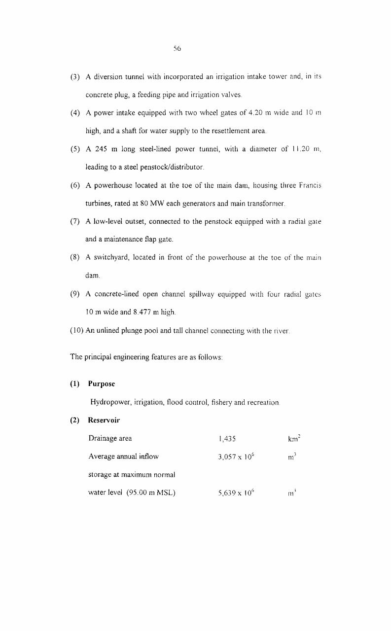
56

(3) A diversion tunnel with incorporated an irrigation intake tower and, in its

concrete plug, a feeding pipe and irrigation valves.

(4) A power intake equipped with two wheel gates of 4.20 m wide and 10 III

high, and a shaft for water supply to the resettlement area.

(5) A 245 m long steel-lined power tunnel, with a diameter of 11.20 11l,

leading to a steel penstockJdistributor.

(6) A powerhouse located at the toe of the main dam, housing three Francis

turbines, rated at 80 MW each generators and main transformer

(7) A low-level outset, connected to the penstock equipped with a radial gate

and a maintenance flap gate.

(8) A switchyard, located in front of the powerhouse at the toe of the main

dam.

(9) A concrete-lined open channel spillway equipped \vith four radial gates

10 m wide and 8.477 m high.

(10) An unlined plunge pool and tall channel connecting with the river.

The principal engineering features are as follows:

(1) Purpose

Hydropower, irrigation, flood control, tlshery and recreation

(2) Reservoir

Drainage area

Average annual inflow

storage at maximum normal

water level (95.00 m MSL)

1,435

3,057 x 106 n1"

111'

57

storage at minimum normal

water level (62.00 m MSL) I 352x10(' m .. ,

Active storage 4,287 x 10(, 1

111'

Reservoir area at max. normal

water level (95.00 m MSL) 185 kmc

Average regulated annual outt10w 3,010 x lOG m]

Probable max-flood (PMF) 5300 1111/S

Maximum water level with PJ\1F 97.48 m MSL

Maximum exceptional water level

(All spillway gates closed, only

fuse dike operation) 98.95 mMSL

(3) Embankments

Crest elevation 100.00 mMSL

Type clay-core rockfill

(4) Main dam and dike no.1

Crest length 909 m

(main dam 761 m, dike no. 1 148 m)

Maximum height on the riverbed 94 In

Total volume 6,514,000 .1 m

(include upstream cofferdam)

(5) Saddle dam

Crest length 708 111

Max. height 50 III

Total volume 1,627,000 .' m

58

(6) Dike no.2 (Fuse dike)

Sill elevation 92.00 mMSL

Crest elevation 97.70 \11 MSL

Max. height 6.00 In

Crest length 106 111

Total volume 8,000 m1

Discharge capacity with water level

at 98.95 (all gates closed) 3,470 ' , III /scc

(7) Dil<:e no.3

Crest length 53 III

Max. height 11 m

Total volume 7,900 1 III

(8) Dike 00.4

Crest length 230 m

Max. height 26 m

Total volume 221,000 m1

(9) Dike no.S

Crest length 160 m

Max. height 20 \11

Total volume 105,000 J m

(10) River diversion

Recurrence internal design flood 500 years

Peak flow of design flood 2,750 1111/S

59

(11) Upstream cofferdam

Crest elevation 48 m MSL,

Total volume 677,000 .1 m

Max. water level for design flood 46.50 111 MSL

(12) Diversion tunnel

Concrete lined internal diameter 10 111

Length 497 m

(13) Routed design flood

Routed design flood with water level

at 46.5 m MSL 1,350 m'/s

(14) Downstream cofferdam

Crest elevation 23 m I'vlSL

Total volume 47,000 m3

(15) Gated spill way

Design flood PMF peak flow 5,300 111~/s

Radial gates (four)

Width 10 m

Height 8.477 m

Spillway sill 87.50 mMSL

Gate top El 95.50 mMSL

Discharge capacity

Reservoir level at El 95.00 m MSL 1,725 m3/s

Reservoir level at El 96.50 m MSL 2,268 m3/s

Reservoir level at El 98.00 m MSL 2,858 3/ m s

60

(16) Low level outlet

Pressure conduit (penstock to gate)

Diameter 6.00 m

Length 53 III

Radial gate

Width 3.00 m

Height 3.50 In

Discharge capacity

Reservoir level at 60.00 m MSL 250 m3/sec

Reservoir level at 80.00 m MSL 320 1113

/ sec

Reservoir level at 95.00 III MSL 365 mJ/sec

(17) Irrigation outlet

Location: Diversion tunnel plug

Pressure conduit

Diameter 0.8 In

Length 24.0 In

Main valve, Howell- Banger type

Diameter 0.8 m

Safety valve, ring follower valve

Diameter 0.8 m

Discharge capacity 10 m3/s

(18) Power intake

Wheel gates (two)

Width 420 111

61

Height 10_00 m

Sill El 44_0 III MSL

Trash rack gross area 500 2

m

Power tunnel (penstock) steel lined

Diameter 11.20 m

Length 270 m

(in tunnel 245 m)

Max. Normal flow 400 m'/s

Penstock branches (three)

Diameter 6_00 m

Length (each) 15.00 m

Design flow (each) 131.00 m3/s

(19) Power" house

Tail water level

Max.lMin. (operating) 15.00/12.00 mMSL

Net head

Max.lMin. 83_50/45.50 m

Max_ flow 400 m3/s

Installed capacity (3 x 80 MW) 240 MW

Annual generation

Primary 484 GWh

Average 554 GWh

62

Average plant faction 0.25

Turbines Three, Francis type

Rated capacity 80 MW

Rated flow 127.40 m3/s

Synchronous speed 176.47 rpm

Runaway speed 355 rpm

Runner diameter 3.80 m

Generators Three umbrella

Rated capacity 89 rv'JVA

Power factor 0.9

Synchronous speed (50 HZ) 176.47 rpm

Fly - wheel effect 6,913

Rated voltage 13 8 KV

Main transformers Three, three- phase

Rated capacity (at 55 degree CC) 89 MVA

Output voltage 230 KV

Powerhouse crane

Capacity: main hoist 2 x 140 tOil

auxiliary hoist 30 ton

63

5. PROJECT DESIGN

A brief description of the main structures and their functions together with the

design parameters and the changes that occurred during the construction stage are

presented here.

5.1 River Diversion

The river Khlong Saeng was diverted through a tunnel on the right abutment so

that, under the protection of the cofferdams, the constructions of the rnaj or structures of th e

project could be carried out in the riverbed. A risk analysis regarding the consequences of a

possible cofferdam overtopping and failure on the densely populated and cultivated areas

downstream influenced a quite conservative to the design of the diversion tunnel.

The tunnel is of 497 m long structure, with a diameter of 10 rn, located within

the right abutment, and can divert a maximum discharge of 1,350 m3/sec

The upstream cofferdam, designed to be incorporated in the main dam, IS of

677,000 m3 rockfill embankment with an impervious upstream clay blanket.

The downstream cofferdam provides the protection to the main construction

area. The upstream end of the tunnel is a bellmounted intake structure that houses t\\/O 10

m high and 5.5 m wide slide gates and lost forms that served for the construction of a first

concrete bulkhead. The permanent tunnel plug incorporates 0.8 m diameter irrigation pipe.

The diversion was closed on April 3, 1986, about two months ahead of the scheduled time,

taking advantage of the good progress of the work and of the very favourable weather \vi th

64

respect to the normal regime of the rains. As it happened the river discharge was at its

lowest point of the year and all the closure operations went on very smoothly

5.2 Dam Embankments

The project requires six embankments, to retain water of the reservoir, plus onc

fuse dike emergency spillway. All six embankments are of the central clay- core rocktill

type.

The embankment vary in height:

Main dam 94 m high

Saddle dam 50 m high

Dike no. 1 35 m high

Dike nO.3 11 111 high

Dike noA 26 m high

Dike no.S 20 m high

The upstream slopes are 1-8 horizontal to 1 vertical in the upper part, 2

horizontal to 1 vertical in the lower part, and the downstream slopes are 1 8 horizontal to 1

vertical.

Design of the embankments was based on a static analysis and a review of'

slopes of similar existing dams elsewhere. In addition, a check was carried out all the

behavior of the embankments during any possible earthquake shaking to ensure, that the\'

would be stable and also not suffer any excessive deformation. The rocktlll was specified

to come from the required excavations for the various structures and from a quarry beside

the spillway tail channel, a few km away from the main dam. The clay was specitled to

65

come from suitable borrow area also a few km downstream of the site of its final

collocation.

The zoning of the embankments was designed to make the best use of the

materials available. The fill was placed in layers of varying thickness depending upon the

grain size of the material; from 0.20 m for the clay up to 1.0 m for the rockfill. The clay is

protected against erosion on the downstream side, by a fine filter and by a transition

containing a significant proportion of fines upstream. Above El. 85.00 on the upstream

side, a fine filter is provided up to the maximum water level (El. 97.5) to allow self-healing

of any cracks that might form in the clay as a result of seismic shaking. On the upstream

face a layer of rip - rap is provided, 3.0 m thick, while oversize rocks (larger than o. I m

size) provided protective layer on the downstream face.

The foundations of the clay cores rest on good sound rock which was treated

by local excavations and filled with concrete, wherever necessary, to prevent the

possibility of any seepage across the interface. The rockfill rests on a foundation of

weathered rock cleaned by bulldozer.

The clay cores form the water-retaining element of the dam in the main dam it

is 4,500 m wide at the base, tapering to 8.0 m wide at the top (El. 99.0). The clay was

placed at moisture content of 1 percent above optimum in the lower part of the dam and 23

percent above optimum, in the upper portion, above El. 58.00, and was compacted to at

least 98 percent of the standard protector compaction.

The rockfill was placed and compacted without sluicing and achieved densities

in excess of 2.2 ton/m3.

66

Fuse Dike

The fuse dike is an inclined thin clay core embankment \vith a grave!

downstream shoulder and rockfill upstream. The embankmellt is designed to be wash <l\vay

if the reservoir level overtops the structure, and provide an emergency spillway in case of

non-functioning or malfunction of the spillway gates. The embankment is 5.7 m high and

has upstream and downstream slopes of 2 horizontal to I vertical and 14 horizontal (0 I

vertical respectively.

Design of the fuse plug was based on a review of similar structures elsewhere

In operation, a low point is provided in the crest, through which water will flow and wash

out the downstream fill, this erosion will also spread laterally and will, in time, remove all

the dike allowing the supporting concrete structure to act as a free-flow spillway.

Cut-Off

~

A grout curtain under the axes of the clay cores provides the cut-off for the

embankments. The grout curtain comprises 2 rows of holes with a maximum depth of

75.00 m in the main dam. In addition, a row of deep consolidation holes is provided 40 III

upstream of the curtain with a maximum depth of 18.0 m in the main dam. The foundation

area below the core is grouted to a maximum depth of 6.0 III to consolidate the surface

treatment of the area.

5.3 Spillway

The spillway, located on the right rim of the reservoir at about 500 m from the

end of dike no. 1 , is of the open chute type, controlled by four radial gates and ending with

67

a ski-jump wherefrom the water will return to Khlong Saeng through a plunge pool and a

discharge channel.

The gated structure is founded on sound rock at E1.76.00 m and is formed by

the ogee structure, with sill at EI.87.50, controlled by four radial gates 10 III wide and

8477 m high, separated by piers 2.50 m thick and 32 III long, with crest at El 100.00

A drainage gallery 2.00 x 2.80 m runs through the weir body, with floor at

E1.78.50; access is provided from E1.100.00 through two vertical shafts 2.00 m diameters,

located in the end piers. The radial gates are articulated over steel trunnions and support

girders embedded into the piers and deeply anchored by pre stressed tendons. Upstream of

the radial gates the piers of the structures are provided with slots for lowering the

maintenance stoplogs.

Pressure equalization on these is done by by-pass valves located in the

discharge gallery. The winches for the operation of the radial gates located on the top of

the piers, at El.l00. In the upstream portion, the top of the piers support also a deck 9.20 III

wide giving continuity to the permanent road connecting all the various parts of the

project.

The chute is formed by an open channel 49.00 m wide and about 5 m deep,

with a gradient of 20 percent along the initial 50 m upstream and 1 I percent along the

remaining 90 m down to the ski-jump, in order to follow the rock profile.

The ski-jump with a cylindrical shape continuous for 27.50 m with 50 In

radius, ends with an angle inclined 20 degree upward, with terminal edge at E1.61.50.

68

The air required for aeration will descend from the spaces remaining naturally

water-free just downstream of the squared-off each pier.

To limit cavitations care has been taken that construction be done without

discontinuity transversal to the flow.

A schematic profile of the spillway chute is given. At about 40 m downstream

of the ski-jump a plunge pools 23 m deep and 120 m long is excavated into the rock for

energy dissipation.

From the plunge pool the water will be returned to the river, through a channel

about 1,500 m long and 100 m wide. During the construction of the dam the following

minor changes were effected to the original design:

(1) Due to the good rock conditions the foundations of the gated structure

have been raised to E1.76.00 from 74.50.

(2) Prestressed tendons have been adopted to anchor the radial gates trunnion

girders.

(3) Following the results of the model tests the bottom elevation of the

channel had been raised to E1.43.00 from 40.00.

(4) The protection slap below the ski-jump had been extended from 12 m to

25 m downstream and had been anchored to the rock by means of tendons

and anchor bars.

69

5.4 Power Intake

The intake structure is located on the right abutment of the main dam, at some

100 m upstream of dike no. 1 center line and adjacent to the inlet of diversion tUllneL It is ;\

58 m high hollow gravity structure, founded on sound rock at E1.42.00 and with top deck at

El. 100.00, encased in a niche excavated into the rock.

The lower portion of the structure forms the real hydraulic intake, with two

funnel shaped sluices changing from 11.75 m x 20.00 m upstream to 4.20 m x 1000 m

downstream and a separating wall 1.S0-m to 2.60 m thick. The ceiling is formed by I-m

thick slab, with 50-cm diameter pressure equalizing holes.

The upstream mouth of the sluices is protected by trashracks 20.00 x 25.00 m

(gross dimensions) supported by two intermediate concrete pillars and two steel beams

filled with concrete. Stoplogs and gates are provided for tunnel closure. The top desk at

EL 100.00 is the service deck, where the gate servomotors are installed and wherefrom the

stoplogs can be operated.

All oleodynamic and electric equipments for gate control is installed inside a

control building located along the access to the intake structure. The control building is a

13.50 m x 5.00 m construction with concrete foundation slab, columns and beams,

masonry walls and removable roof made of steel trusses and steel sheeting. During the

construction, the following minor changes were made to the original design.

(1) Two additional wmg walls have been built to contain a pOl1ion of the

definitive backfill and consequently to speed up the erection works for the

anticipated diversion tunnel closure;

70

(2) An additional shaft had been introduced to contain the system of pipes and

valves for the resettlement area water supply.

(3) The control building had been moved about 20 m downstream, to base it

on sound rock and also eliminate two lateral retaining walls.

5.5 Power Tunnel and Penstoci{

The power tunnel, excavated through sound rock, is abollt 245 rn long with (\

gradient of about 16 percent and with a minimum rock cover of about 20 m.

Excavation cross-section is horse shoe shaped, with a 6.4-111 upper radius

Conventional rock supports had been procured, to be used as required. As it happened,

very little support was used.

The finished cross-section is circular with 11.20 m inside diameter, fully steel

lined. The lining is designed to be self-resistant both for internal and external pressures,

including contact grouting at 5 kg/cm2

The gap between the steel lining and the rock is filled with concrete, with Cl

systematic pattern of consolidation and contact grouting at 5 kg/cm2 pressure, from inside,

The power tunnel ends about 30 m from the powerhouse, from that point dov.'1l

to the opposite end of the powerhouse, the penstock was installed in the open encased in

concrete and then buried under the backfilI forming the powerhouse esplanade.

The penstock diameter is maintained constant at 11.20 m from the tunnel outlet

to the powerhouse, and then gradually reduced from 11.20 m to 6.00 111, with three

identical branches, at 55 degrees, feeding the turbines.

71

The concrete encasement, runnlIlg along the powerhouse, has been rigidly

connected with it in order to act as a balancing arm or counterweight, contributing to the

stability of the powerhouse upstream wall.

All concrete encasement is divided in blocks, with contraction joints grouted

after concrete shrinkage. Similarly, the contraction joint between the distrihutor

encasement and the powerhouse is grouted in such a way that the two structures practically

form a monolith. Downstream of the last branch pipe, the distributor ends with an

expansion joint, which is in its turn connected to the l0w level outlet. The joint is designed

in order to allow relative displacement between the two structures, either for thermal

effects on differential settlements. The concrete encasement of the joint forms a 4.00 m x

100.00 m x 100.00 ill room, access to which is provided from the powerhouse through a

watertight door, designed for the full head up to the maximum reservoir water level.

5.6 Low Level Outlet

The low level outlet is essentially a sluice inclined some 20 degrees upward,

steel lined connected upstream with the penstock and discharging into the tailrace channel

downstream with the terminal flip edge at El. 24.50 and chute slab down to El. 11.00.

The sluice is controlled by a radial gate operated by servomotors installed on a

service deck El. 33.40 above the gate. The trunnion support girder is fitted to the lateral

piers by prestressed tendons anchored 25 m deep into the concrete.

Maintenance of the radial gate can be done after closing a pressure flap gate

installed just upstream of it, operated by a servomotor installed at El. 3100 inside Cl

72

cellular construction, rising up directly from the lining encasement up to the service deck

at El. 33.40.

Above the servIce deck in a control building house the oleodynamic and

electric equipment controlling both the flap and radial gates. During the construction the

wing wall in the right side of the outlet was extended up to the outlet of the diversion

tunnel. No other significant changes were made.

5.7 In"igation Outlet

The purpose of this facility is to guarantee a constant minimum \vater rei east:

of 10m3 /s for irrigation needs even when the power tunnel is closed and the reservoir level

is lower than the spillway sill (El. 87.50).

The facility includes the following structures:

The irrigation intake structure, built above the diversion tunnel inlet, just

downstream of the concrete inlet plug.

The upper diversion tunnel stretch, about 124 m long, upstream of the

tunnel plug.

The feeding pipe embedded in the diversion tunnel plug.

The outlet structure, built inside the diversion tunnel just downstream the

plug.

The lower diversion tunnels stretch, about 390 m long, down to the

tailrace channel.

5.8 Powel'house

The powerhouse is located on the right bank of the river, just downstream of

the main dam, parallel to the original river bed. It is an outdoor structure ()40 111 x 430 rn

in plan and 58 111 high, founded on sound rock at El. -7.50, housing three generating units

and all auxiliary services, the erection area, the administration building and other facilities

Structurally the powerhouse may be divided into two parts:

The substructure, from the foundation up to served deck at E. I. 33 AO

The superstructure above the service deck

The service deck has been fixed at E1.33.40 with a 0.50-m free board above the

maxImum possible tailrace water level corresponding to the Probable Maximum Flood

(PMF).The superstructure, formed by reinforced columns and beams, with thin perimetral

closure walls, is fully exposed.

The substructure formed by a heavy reinforced concrete structure, is either

buried under backfill on the upstream side or exposed on the downstream side facing the

river. In order to account for thermal shrinkage, the powerhouse has been divided in to f()ur

different blocks, one per each unit (20.50-18.00-26.50m long respectively) and one for the

erection area (29.00 m long), separated by contraction joints. The joints are sealed by \vatcr

stops and provided with shear keys from foundation up to deck at El. 33.40.

After concrete shrinkage, the joints have been fully grouted up to El 20.00 thus

turning the substructure practically monolithic. Above EI.20.00, conventional contraction

joints are provided, with water stops from EL 20.00 to 33.50.

74

5.9 Switchyard

The switchyard is located on the left abutment of the river, just downstream or

the main dam, opposite to the powerhouse, with the finished top surface at El. 40.00. It is a

25,000 m2 area divided into:

A 230 kv sector, with three overhead lines connected to the step-up

transformers at the powerhouse, and two outgoing transmission lines with the possible

future extension of two more.

A 115 kv sector, connected to the 230 kv sector through a tie-autotransformer

with possible future installation of a second one, in case of expansion, and two outgoing

transmission lines with the possible future extension of three more.

A small 33 kv sector, connected to 230 kv sector through a transformer with

two outgoing transmission lines with the possible future extension of one more.

The control building is located roughly at the center of the switchyard, between

the 230 kv and 115 kv sector connected to the powerhouse by a cable gallery, 2 20 m x

2.50 m x 335 m long, with upper outer face 1.00 m deep under the ground surface.

From the control room depart two main cable trenches which branch out in a

three levels trench network, distributing the cables to the outdoor equipment. All cable

trenches are in reinforced concrete, 1.20 m x 1.30 m - 1.20 m x 0.90 m - 0.80 m x 0.90m -

0.25 m x 0.25 m respectively, with top edges at O. 10 m above the finished ground surface

of the switchyard, covered by checkered plate covers. The ground surface of the yard, out

of the roads width, is finished by OAO m thick gravel layer.

75

6. COSTS AND PROGRAMMES

6.1 Estimate and Project Evaluation

6.1.1 Early Studies

The feasibility report was prepared under an agreement economically self­

supported by ELC, and the definite study was negotiated with EGA T on a fixed sum basis.

These activities were carried out between 1978 and 1981.

6.1.2 Project Feasibility

The feasibility of the report was established on the basis of an installed

capacity of 240 MW, an average annual runoff of 3,000 mcm, a live storage volume of

4,300 mcm, and an average energy output of 554 Gwh.

6.1.3 Project Benefits

From the implementation of the Rajjaprapha dam a senes of benefIts v,'ere

expected they are:

Generation of electric power

Increase of agricultural output as a result of irrigation.

Additional fishery output from the lower river section as well as from the

reservoIr.

These were the quantitative benefits on which the feasibility of the project \vas

estimated.

76

(1) Power generation benefits

The power benefits were estimate in companson with an alternative thermal

plant to be located in the same region to meet the forecast demand of energy.

The thermal alternative consisted of a combination of oil fired and gas turbine

power. The reference fuel prices were based at the time on a cost of US$ 14 to 18 per

barrel of crude oil. Since then the costs have reached a maximum of US$ 34 per harrel and

minimum of US$ 10 to 12 per barrel. At that time they were around USS 16 to I g per

barrel and the trend is towards a moderate increase over the years: basically the calculation

can be considered still valid.

(2) Irrigation benefits

When full production is achieved in the 23,100 ha of net irrigated land, the

total irrigation benefits will amount to about p 420 million per year. It is considered that

the irrigation benefits will materialize gradually over a period of five years after the

completion of the works in each irrigation district.

(3) Fishery benefits

The fishery benefits were evaluated at ~ 27 million per year. It is assumed that

they will start to materialize on the second year after reservoir filling, The time needed to

get full fishery benefits is estimated in four years.

77

(4) Total benefits

On the basis of the costs estimated and of the benefits that were to be derived

from the Rajjaprabha dam, the classic parameters usually adopted to assess the feasibility

of a project clearly indicated that the project was economically attractive

The internal rate of return (IRR) of the project is 16.2 percent.

The benefit cost ratio CB/C) for i :::: 10% is 1.60.

On the basis of these parameters the deci"ion was made to proceed with the

implementation of the project. Since that time, as it explained were below because of \'ery

favorable concurrence of circumstances, the actual prices of the various contracts were

extremely competitive and the actual costs of the project was lower than the estimate, thus

confirming once more the extreme economical soundness of Rajjaprabha multipurpose

project.

6.1.4 Contract Design and Tender Documents

The agreement for the preparation of the contract design drawings and tender

documents was formally signed on November 20, 1981. However, the work had already

been started various months earlier, with the Inception Mission. The work was carried out

by ELC - Electroconsult in joint venture with SEA TEC (South East Asia Technology Ltd.)

and was completed in about one year; and the negotiated cost was US$ 1,496,150 and ~

6,216,000.

78

6.1.5 Cost of Construction and Supenrision of the Contracts

The cost estimate was based on detailed analysis carried out 011 the costs of tile

mam works for the project; due consideration was given to current projects under

construction in Thailand and in South East Asia.

The basic criteria for construction of the major items of work were defined and

schedules of quantities were prepared together with an assessment of the equipment to be

installed. From the detailed cost estimate that was prepared, the project cost came to a total

amount slightly less than j3 5,900 million equivalent to US $ 290 million, including interest

during construction. As it is normal in major projects, the cost estimate was made both in

foreign currency and local currency.

It was assumed that the foreign currency portion would cover, mainly:

(l) Power Station equipment

(2) Construction plants, with the relative spare parts when imp0I1cci.

(3) Special construction equipment.

(4) Hydraulic equipment gates and cranes.

(5) Explosives, additives and special paint.

(6) Instrumentation and controls.

(7) Supervision, overheads and profIts of foreign contractors.

(8) Engineering services by foreign consultants.

The local currency portion would cover mainly;

Cl) Construction plant and equipment available in Thailand.

79

(2) Cement, fuel, and reinforcing steel, tiles and other materials.

(3) Fabrication and erection of permanent equipment in Thailand.

(4) Resettlement costs

(5) Salaries and wages

(6) Overheads and profits of local contractors

(7) Import duties and taxes

(8) EGAT administration

During the preparation of tender documents, agreement was reached on the

number and type of contracts to be tendered. In an effort to keep the original project

implementation schedule, the civil works were divided into two contracts : one for the

diversion tunnel and apartment work, and other for the main civil works, which included

dams, powerhouse, power conveyance works, flood control works and works relating to

switchyard.

The electromechanical works were divided into six contracts: (i) for hydraulic

equipment including tunnel lining, penstocks and all the hydraulic gates (ii) for tardiness

and generators (iji) for power plant equipment (iv) power station cranes (v) for switchyard

equipment and (vi) for transformers and lighting arresters.

The cost estimate was revised in 1981 to an amount of 13 7,C)3 5 million

equivalent in view of some changes that were decided and presented to the cabinet, which

approved it in February 1982.

80

6.2 Source of Funds

The budget adopted for Rajjaprabha dam was composed of both foreign and

Thai currencies. The foreign currency portion was financed with loans tJ·OIll the

International Bank for Reconstruction and Development (World Bank), the Organization

of Petroleum Exporting Countries (OPEC) and the Kuwait Funds for Arab Economic

Development (KFAED).The national currency portion was financed by Thai Government

subsidy and EGA T' s own revenue.

6.3 Actual Expenditure

It has been described in section 6.1 how the initial cost estimate was revised in

view of the changes to be approved by the cabinet. The final project cost estimate was

updated considering the extra costs due to additional works that would be necessary during

the construction period, and also the variations in quantities with respect to the confidential

estimates prepared for the tender documents. In the end, the total direct cost of USS 171.36

million equivalent (}1 4,313.96 million equivalent) turned out to pe an exceptionally low

cost for a medium size hydroelectric project like Rajjaprapha dam. 1 n fact, the cost per

kilowatt installed is in the order of US$ 714, on extremely low cost for any type of power

generation, and especially for a hydroelectric project that is normally characterized by high

initial investment and low operation and maintenance expenses .

•

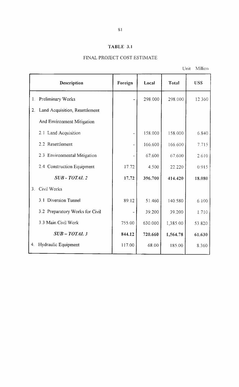
81

TABLE 3.1

FINAL PROJECT COST ESTIMATE

Unit \1illioll

Description Foreign Local Total US$

1. Preliminary Works - 298.000 298.000 12.360

2. Land Acquisition, Resettlement

And Environment Mitigation

2.1 Land Acquisition - 158.000 158.000 6.840

2.2 Resettlement - 166.600 166.600 7715

2.3 Environmental Mitigation - 67.600 67.600 2.610

2.4 Construction Equipment 17.72 4.500 22.220 0.915

SU13- TOTAL 2 17.72 396.700 414.420 18.080

.., Civil Works .J.

3.1 Diversion Tunnel 89.12 51.460 140.580 6.100

3.2 Preparatory Works for Civil - 39.200 39.200 1.710

3.3 Main Civil Work 755.00 630.000 1,385.00 53.820

SUB- TOTAL 3 844.12 720.660 1,564.78 61.630

4. Hydraulic Equipment 117.00 68.00 185.00 8.360

82

TABLE 3.1 CONTD

Description FOI'cign Local Total USS

5. Electro Mechanical Works 185.00 i I

5.1 Turbines and Generators 615.90 46.00 885.90 31 270

5.2 Powerhouse Cranes 13.66 1.90 15.10 0.600

5.2 Transformers and Lighting A 60.50 4.60 65.10 2.540

SUB-TOTAL 5 854.06 52.50 905.56 34.410

6, Transmission System

6.1 Switchyard Equipment 59.10 18.10 77.20 2900

6.2 Transmission System 220,00 100.80 320.80 1 I. 960

SUB- TOTAL 6 279.10 118.90 398.00 14.860

7. Engineering Services 251.30 99.90 351.20 13.855

8. EGA T Administration - 196.00 19600 7805

TOTAL DIRECT COST 2,363.30 1,950.66 4,313.96 171.360

9. Import Duties and Taxes - 347,54 347.54 13.175

10.Interest During Construction - 638,50 638.50 22.683

TOTAL PROJECT COST 2,363.30 2,936.70 5,300.00 207.218

Source From completion report of "Rajjaprabha Multipurpose Project.

CHAPTER IV

PHYSICAL RESOURCES

CHAPTER IV

PHYSICAL RESOURCES

1. INTRODUCTION

The physical environment relating to a mUlti-purpose dam project are classified

into climate, water, and land resources. These physical resources may either cause effects

to or are affected by the project at different levels, time and locations. The physical

resources of the Rajjaprabha dam presented in this chapter are: (i) climate and surface

water hydrology (ii) ground water (iii) water quality (iv) soils and land capability (v)

mineral resources (vi) erosion and sedimentation and (vii) salinity intrusion.

A review of existing physical environmental resources and the evaluation of

the impact of the dam on such resources are considered necessary as they are expected to

produce favourable as well as harmful impacts on human use values and quality of life.

2. CLIMATE AND SURFACE WATER HYDROLOGY

2.1 Introduction

The Phum Duang river basin is located in the upper southern part of Thailand.

Its area extends from the coastilne of the Gulf of Thailand in Surat Thani province in the

east to Phang-nga province in the west. The climate is tropical monsanic, being

characterized by rather high temperature and humidity all year round with markedly

seasonal distribution of abundant rainfall. It is influenced strongly by both the northeast

and the southwest monsoons.

84

2.2 Objectives

Main objectives of this climate and surface water hydrology study are:

(a) To survey the existing status of climatologic and hydrology gaug1l1g

station in the river basin.

(b) To update relevant climatic parameters and stream flow data at selected

status using data since 1978 up to the latest possible.

(c) To assess trend and potential climatic changes between the pre-and post­

impoundment periods.

(d) To assess changes in flow conditions betwecn the pf(~-and post

impoundment periods.

2.3 Methodology of Study

The study was carried out based on the available data and information in the

project area. The general climatic conditions of the region were reviewed. Locations of the

observation stations and the available records were searched from the govcrnmental

agencies concerned. Additional data of recent years were collected from the field office in

order to get the most up to date picture of the environment.

These data were analysed to determine their statistical characteristics, including

the temporal and a real distributions. The results were then interpreted and described as

related to the Rajjaprabha dam.

85

Gauging Station

There are 8 climatologic stations and 8 stream gauging stations in the Phutn

Duang river basin which are in operation. Locations of these stations are shown in Figure

4.1. The pre-impoundment perid (or pre-dam) is taken as the period before water year

1987, and the post-impoundment period (or post-dam) is taken as the period from water

year 1987 till water year 1997.

These data were analyzed to determine their statistical characteristics,

including the temporal and real distributions. Probable effects of the project on the climatic

parameters or vice versa were then evaluated based on the literature revicw, experience and

the interpreted results.

2.4 Results of the Study

The study reveals that after about ten years of its existence the Rajjaprabba

dam has not produced any significant changes in climatic features found. Whatever minor

differences are found in climatic parameters arc largely due to their pertinent stochastic

nature. Surface water has, on the contrary, been modified by the regulation effect of thc

Rajjaprabha reservoir. Such regulation gives rise to bettcr utilization of the water from the

Phum Duang river.

Comparisons of the climatic parameters and streamflows experienced during

the pre-impoundment period and the rather short post-impoundment period are as fo11O\\ls.

86

t.r\1;:>h()~ Cncl 0

•

•

N

~ __ -4~~ __ -D~ __________ -+ ____________ ~~~~~ ______ --.~~u~ 'r~\~ ____ ~ ______ --;

,~~

Kopon

Basin Balll/dory

Sr;b!JosJn Boundary

Klliono crnd River

~ Slream Gtl9J[~O SlariC(,

• • •

FIGURE 4.1

• Amphoe Khl1n Tho,e

\1 ~ 10 r5 ZO Km ---­GRAPHIC SCALE

PHUM DUANG RIVER BASIN AND GAUGING STATION

87

2.4.1 Rainfall

Temporal distributions of rainfall over the year during the two periods \VC1"C

similar, with heavy rains during September to November and light rains during January to

March. Mean annual rainfall over the whole basin increased by about 4.01% from about

2,024 mm during the pre-impoundmcnt period to about 2,106 mm during the post­

impoundment period (Table 4.1). The mean annual rainfall over the Rajjaprabha catchment

area slightly increased from about 2,035 mm during the pre-impoundment to about 2,087

mm in the post-impoundment period (Table 4.2).

2.4.2 Evaporation and Temperature

Mean annual evaporation of the Rajjaprabha catchment area is estimated to

vary slightly during the two periods, from about 1,337.7 mm during the pre-impoundment

period to about 1,457.2 mm during the post-impoundment period. The variation is shown

in Table 4.3. Temperature, and other climatic features at the dam site experienced during

the two periods were almost identical. While relative humidity varied from 52 percent to

98 percent, and air temperature form 14 QC to 39 QC, (Figure 4.2).

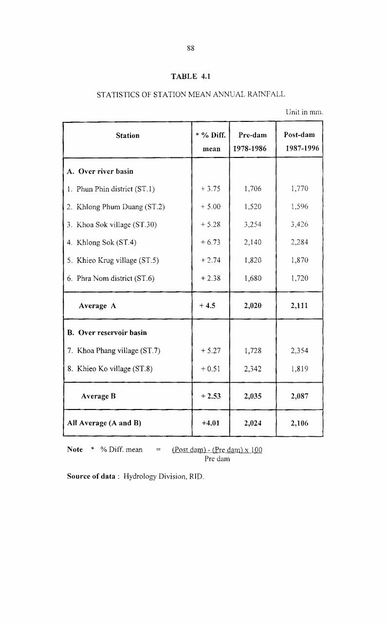
88

TABLE 4.1

STATISTICS OF STATION MEAN ANNUAL RAINFALL

Station

A. Over river basin

1- Phun Phin district (ST.l)

2. Khlong Phum Duang (ST.2)

" Khoa Sok village (ST.30) -'.

4. Khlong Sok (ST.4)

5. Khieo Krug village (ST.5)

6. Phra Nom district (ST.6)

Average A

B. Over reservoir basin

7. Khoa Phang village (ST.?)

8. Khieo Ko village (ST.8)

Average B

All Average (A and B)

Note * % Diff. mean

* % Diff. Prc-dam

mean 1978-1986

+ 3.75 1,706

+ 5.00 1,520

+ 5.28 3,254

+ 6.73 2,140

+ 2.74 1,820

+ 2.38 1,680

+ 4.5 2,020

+ 5.27 1,728

+ 0.51 2,342

+ 2.53 2,035

+4.01 2,024

(Post dam) - (Pre dam) x 100 Pre dam

Source of data: Hydrology Division, RID.

Unit in mm.

Post-dam

1987-1996

1,770

1,596

3,426

2,284

1,870

1,720

2,111

2,354

1,819

2,087

2,106

89

TABLE 4.2

AVERAGE ANNUAL RAINFALL OVER RESERVOIR AND RIVER BASIN

Average rainfall over Reservoir Average rainfall over river

Month (mm) (mm)

Pre-dam Post - dam Prc- dam Post - dam

1978 -1986 1987 - 1996 1978 - 1986 1987 - 1996

Apr 56.7 90.8 73.8 54.5

May 156.1 198.2 182.3 281.2

Jun 147.0 163.7 151.5 139.7

Jut 190.7 147.4 192.7 231.7

Aug 83.6 164.8 168.8 197.6

Sep 132.6 240.6 220.9 290.4

Qct 547.7 370.4 328.0 570.5

Nov 394.2 383.7 338.6 550.5

Dee 92.0 192.8 251.0 227.2

Jan 20.1 69.5 49.0 65.1

Feb 10.4 36.8 45.6 54.5

Mar 9.2 28.7 22.3 24.6

Total 2,035 2,087 2,024 2,106

Note

Source

* A veraged from two stations : ST 7 and ST 8

** Averaged from six stations: ST 1, ST2, ST3, ST4, ST5, and ST 6

Meteorological Department.

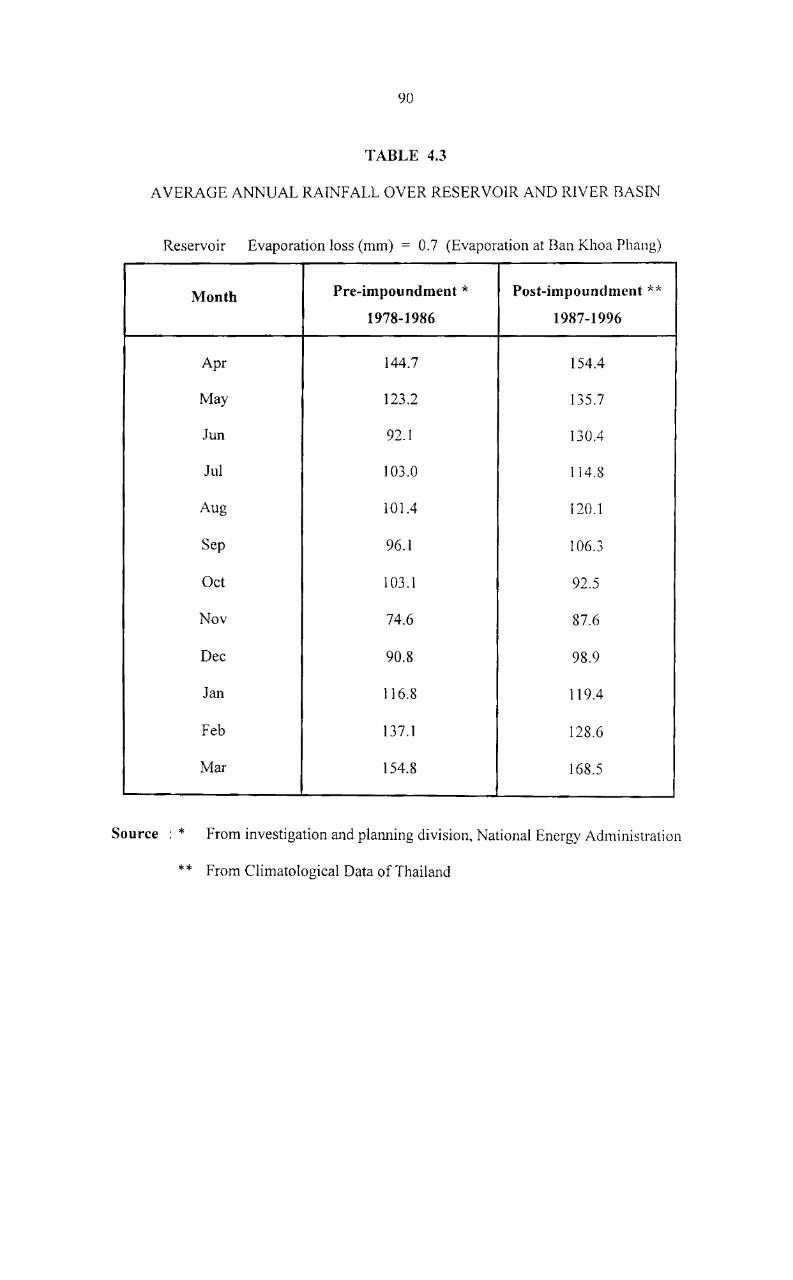
90

TABLE 4.3

AVERAGE ANNUAL RAINFALL OVER RESERVOIR AND RIVER BASIN

Reservoir Evaporation loss (mm) = 0.7 (Evaporation at Ban Khoa Phang)

Month Pre-impoundment * Post-impoundment ** 1978-1986 1987-1996

Apr 144.7 154.4

May 123.2 135.7

Jun 92.1 130.4

Jul 103.0 114.8

Aug 101.4 120.1

Sep 96.1 106.3

Oct 103.1 92.5

Nov 74.6 87.6

Dec 90.8 98.9

Jan 116.8 119.4

Feb 137.1 128.6

Mar 154.8 168.5

Source . * From investigation and planning division, National Energy Administration

* * From ClimatologicaI Data of Thailand

91

f---. 1---_ r-- r---. EX! Mo .. ·:irrum / --- .--f.-- 1--- r" j- -- .. /

.............. "- Mean Maximum /...-/

u 30 0 T-- /

QJ~ ... -- ---.- - Milan ::J -0

- --:... ---t,.\eon iv',inimum - ---... " a. E 20 ~ ~-

f-.-...... f-' .. - -----_ .

- r-- r--- -~--" r----.... J/ '\ V'- Ext. Minimum ~

~ I :...,.------10 M A M JJ A. SON D J F M

A. Temperature

r--- 1---- -- 1--- --- r----I----,..-------I----f----~ 90 1---+--4--+-+--+--+--1----+--+--+--+--1 >-

Cl)

a:: 60 V 50 ..--

M A M J J A S o N o J F M

Month

B. Humidity

LEGEND: Mean maximum

Mean

Mean minimum

FIGURE 4.2

MONTHLY CLIMATICS STATISTICS AT SELECTED STATIONS

SURROUNDING KHLONG PHUM DUANG REGION

92

2.4.3 Surface Runoff

At Rajjaprabha dam site the distributions of mean monthly stream flow during

the two periods were of similar pattern. Hydrograph of the monthly flO\v comprised two

peaks. the lower one in May and the higher one in November. Low f10ws were observed in

March and August. Mean annual flow at the dam site increased slightly from about 3,038

mcm observed in the pre-impoundment period to about 3,057 mcm. And further

downstream at the town of Surat Thani the mean annual flow increased by about 12.8 %

during the two periods, from about 6,411 mem to about 7,232 mcm (Table 4.4).

TABLE 4.4

ANNUAL STREAMFLOW PRE-AND POST DAM IN TI-IE WATERSHED AREA

Annual Stream flow

Location Area (kru2)

Pre - dam Post - dam

Catchments area 1,435 3,038 3,057

River basin area 4,668 6,411 7.232

Source Hydrology Division, Royal Irrigation Department.

93

3. GROUND WATER RESOURCES

3.1 Introduction

Ground water development in the Phul1l Duang river basin is rather limited.

From 1974 to the present day only about 386 deep wells have been drilled in the area. Most

of them are used for domestic water supplies in rural communities, and only a fc\\' arc used

for municipal and urban water supplies. None has been used for irrigation purpose.

Shallow wells or hand-dug wells are commonly used for domestic water supplies in almost

every village of the study area. The main reason of not using ground water for irrigation is

plentiful availability of surface water in the area, where the average annual rainfall varies

from approximately 1,596 mm to 3,426 mm (Team Consulting Engineers, 19RO).

Nevertheless, from water resources management view point ground water resource in the

basin is still important. It serves as water supply sources for small towns and rural villages.

and also provides supplementary irrigation water to tree crops and vegetables during dry

seasons.

3.2 Objectives

The objectives of ground water study are to assess the impact of water

impoundment in Rajjaprabha reservoir on ground water resources:

(a) The use of ground water as a source of domestic water supply for

communities in the rural areas.

Cb) The use of ground water as a supplementary supply for dry season

croppmg.

94

(c) The change in ground water hydrological conditions due to the project

implementation affecting soils internal drainage and soil capability.

(d) The effects of salinity intrusion and flood control on ground water

resource development.

3.3 Methodology of Study

To achieve the above objectives the following methodology of study has b~en

used:

(1) Collect data on water table, water quality, hydrological maps, and inventory

of ground water utilisation from the Department of Mineral Resorccs, Otlice of

Accelerated Rural Development, Public Works Department, and Provincial Water Works

Authority.

(2) Assess the ground water resource conditions from collected data to verify

pattern of chages after the project implementatoin for both upstream and downstream

areas. The assessment includes ground water level, yield, utilisation, quality, water logging

seepage from/into the reservoir, and the effects of salinity intrusion and flood control on

ground water resource.

(3) Observe ground water levels in the irrigation area and the area just

downstream from Rajjaprabha dam in order to identify changes in ground water level from

the pre-impundment period. This, is used as the basis for the assessment of soil capability,

water logging problem, and seepage from the reservoir.

95

3.4 Results of the Study

3.4.1 Ground Water Geology

Water bearing formations in the watershed area are broadly classified into

unconsolidated and consolidated formations. The unconsolidated formations, or aquifer,

found in the gulf coastal plain region consist of unconsolidated gravel, sane! and clay of

fluvial origins. Beach sand aquifers of the unconsolidated group, generally Vv'ith less than

about 7 m thick, are found in the coastal areas. Consolidated aqui fcrs encountered in the

upstream hilly and mountainous areas are of carbonate. metasediment, metamorphic, ~nd

granitic rocks. These aquifers are recharged by rainfall and inundated water from nearby

streams at locations where hydraulic connections to the aquifers prevail.

3.4.2 Ground Water Availability

Ground water availability vanes considerably in the project area mainly

according to the prevailing types of aquifers. High availability potential areas, with a well

yield of more than 50 cmlh are in the flood plain of Phum Duang river in the easthern part

of Muang district of Surat Thani province, with unconsolidated aquifer covering Muang

district. Lower availability potential areas with a well yield from 20-50 cm/h are also of

unconsolidated aquifers in Muang district, Phun Phin district, and a portion of Chaiburi

district. The remaining upstream area has the least availability potential, less than 20 cm/h

well yield (Department of Mineral Resources, 1981). The number of deep wells in the

watershed area is as shown in Table 4.5.

96

TABLE 4.5

THE NUMBER OF THE DEEP WELLS DRILLED DURING 1974-1996 IN TI lE

WATERSHED AREA

Location Pre-dam Post.dam

Total 1974-1986 1987 - 1996

1. Upstream area

Ban Ta Khun district IO 24 34

Phrase Nom district 8 17 j-_J

Sub total 1 18 41 59

2_ Downstream area

Khirirathana Nikhom district 22 66 88

Phun Phin district 25 91 116

Muang Surat Thani district IO 113 123

Sub tota12 57 270 327

Total 75 311 386

Source Ground Water Division, Department of Mineral Resources

97

3.4.3 Ground Water Utilization

As ground water in most of the project area is of acceptable quality for lIse as

drinking water, it is presently used mainly for domestic water supplies. It is an important

source of water supply for rural villages. More than 380 tube wells were drilled during

1974 to 1996 by government offices responsible for rural water supply development.

About 98,400 m3/day of water is estimated to be exploited from the ground water in the

project area, about 24 % of which is from wells in the rural villages (Ground Water

Division, 1996). Use of ground water for irrigation i~ rather limited as other convenient

and economical sources are mostly available. Ground water is, hoyvever, the main source

of supplementary water during dry season for deep rooted tree crops in the project area.

(Table 4.6)

3.4.4 Ground Water Levels

Effects of the Rajjaprabha dam and other projects on ground water after this

short period of impoundment and river flow regulation are not conclusive. Although

relatively high ground water level are observed in this study in the downstream irrigation

area, 1.0-2.5 m below ground surface, it is not likely to be the results of irrigation as shown

in Table 4.7. This inference is based on the fact that application of irrigation water has only

recently begun and that too only in a limited area.

Besides, improved drainage due to the newly implemented drainage system,

together with the regulation effects of the Rajjaprabha reservoir, should pose a decreasing

trend on the ground water level in the irrigation area. Although reported to have increasing

trend in ground water level, no systematic record of water level exists for the dug wells

98

locating just downstream from the storage darn. Hence the effect of this project on ground

water, as reasonably anticipated in the pre-impoundment environmental and ecological

study, should be further assessed in post implementation period.

TABLE 4.6

UTILIZA TION OF DEEP WELLS DRILLED

No. of wells Domestic Organization

Drilled (Hand Pump) Dug wells

Department of Mineral 131

Resources

Department of Health 8

Office of Accelerated Rural 120 386 wells 250 wells

Development 72.600 m 3/day 25,800 m3/day

Department of Civil Work 64

Other Agencies 63

Total 386

Source From Office of Accelerated Rural Development, Ministry of Interior.

TABLE 4.7

COMPARISON OF GROUND WATER LEVELS IN THE WATERSHED AREA

AFTER WITH THOSE OBSERVED IN THE PREVIOUS INVESTIGATION

Location Water level Below ground

(May) (August)

Upstream area

1. Khoa Phang village 1.00 0.70

(1.20) ( 1.00)

2. Bang Kaew village 0.80 0.60

(1.20) (0.90)

3. Pattana village 1.00 0.80

(1.50) (1.20)

Downstream area

1. Hat Khan village 1.20 1.00

(1.50) (1.10)

2. Pong village 1.40 1.80

(1.80) (2.20)

3. Phun Phin district 1.50 l.80

(1.80) (2.50)

Notes

Source

Number in parentheses is previous investigation

Survey data

Surface (m)

(January)

1.50

(2.00)

1.20

(1.60)

1.50

(2.20)

1.80

(2.40)

2.20

(1.40)

2.1 ()

(2.50)

100

3.4.4 Effects of Salinity Encroachment and Flood control on Ground water'

Resource

In the coastal area of the PhU111 Duang river basin, the Beach Sand Aquifers are

in hydraulic continuity with seawater. The lowering of ground water level can result in the

encroachment of seawater. This will result in degradation of water quality in the basin or a

portion of the basin due to the intruded seawater. There are several means for controlling

the encroachment, but the most practical one is by adopting proper exploitation in the

coastal area. The Beach Sand Aquifers along the coastal area are not over 6 111 thick and

yield 5-10 gpm. So in order to control seawater encroachment in the area, the depth of \vell

should be too deep to avoid encountering salt water, and the pumping rate should not be

over 5 gpm.

Rajjaprabha reserVOlr operation regulation for flood protection to the

downstream flood prone area has resulted in reduction in flood peak discharge at Phul1

Phin district. This will reduce ground water recharge potential in the downstream area due

to less recharge area and shortened recharge period. However, the flood prone area will be

used mainly as paddy fields, hence flooding on the land surface can still be expected

during many months in a year. In this case the recharge area and recharge time may not be

much different from the condition without flood control scheme.

3.5 Conclusion and Recommendation

In fact, the creation of a storage reservoir will not affect the ground water

geology of the area, but it will affect the movement of ground water, i.c. watcr table and

recharge.

101

However, at this stage of investigation the water impoundment of Rajjaprabha

reservoir seems not to have any serious effects upon ground water resources. In order to be

able to make quantitative assessment in the next stage of post environmental evaluation

study, monitoring program to measure water levels both in the area just dO'vvl1stream from

the dam site and irrigated area should be set up.

102

4. WATER QUALITY

4.1 Introduction

After the Rajjaprabha dam was put into operation in 1987. it was expected that

the water quality would chage sigificantly from the pre-impoundment investigation results.

The water in the hypolimnion was expected to be rich in organic materials, nutrients, and

inorgaic salts. Reservoir releases, which will be low in oxygen and high in iron and

mangaese, would be unfavourable to the growth of livig organisms. However, thermal

stratification was expected to be mild and therefore should not cause any sigificant

problems. An enquiry was conducted to see whether this claim to true or not. This section

presents the results off field investigation for water quality conducted, after the reservoir

has been put into operation

4.2 Objectives

follows.

The mam objectives of monitoring of water quality 111 this project are as

(a) To monitor seasonal variation of reservoir water quality as well as the

reservoir ecosystem.

(b) To monitor seasonal variation of surface water quality along the Phul11

Duang river, downstreanl from the dam downward to the river mouth.

(c) To evaluate the extent of change in water quality and their effects on

environmental parameters.

103

4.3 Field Investigation

Two field investigations were conductcd, the first in the dry season (during 1-7

April 1997), the second in the late rainy season with a higher amount of rainfall during 15-

20 November 1997).There are four gauging stations as shown in Figure 4.3. The water

quality for the three investigations can be concluded as follows.

4.4 Results of the Study

Water quality in the reservoir has changed significantly from that recorded in

1980 before the impoundment. Mild thermal stratification has occurred in the reservoir.

Dissolved oxygen is high in the circulating top layer (epilimnion), and decreases with

water depth until it is depleted below the thermoclinc. The watcr in the hypolimnion is

relatively rich in organic materials, nutrients and inorganic salts. But living organisms do

not exist in the bottom layer due to lack of dissolved oxygen, and to some extent due to the

presence of hydrogen sulfide. With regard to the overall water quality in the reservoir, it

can be concluded that the water quality in the epilimnion (0-5 m layer) and the

mesolimnion (5-15 m layer) is very clean. It is suitable for use as a source of "vater supply,

for recreation, and can support aquatic life. In the hypolimnion, which is from 15 111 depth

to the bottom, oxygen is absent and a great amount of hydrogen sulfide gas prevails.

Although this results in minimizing corrosion of the steel lining of the outlet works, there

is strong hydrogen sulfide odour stripped from the reservoir release. This nuisance odour

will remain for some time, until the biodegradation at the reservoir bottom is completed.

The water quality of the gauged stations both the pre-and post impoundment as shown in

Table 4.8 and 4.9 respectively.

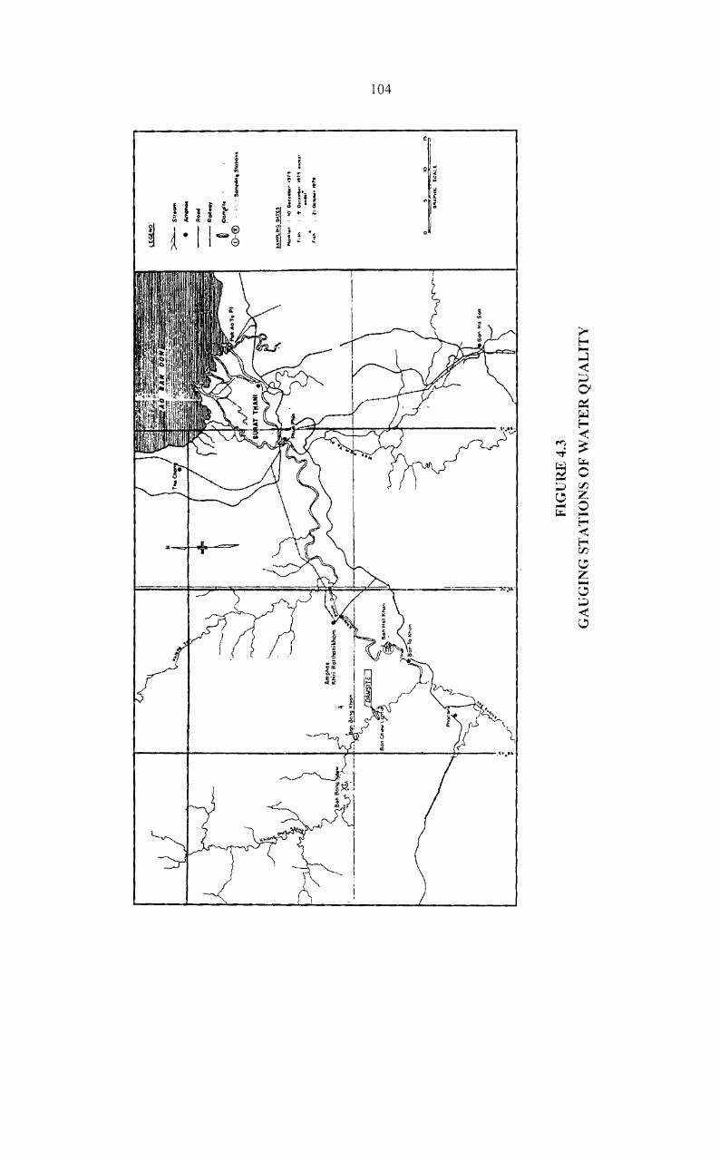
FIG

UR

E 4

.3

GA

UG

ING

ST

AT

ION

S O

F W

AT

ER

QU

AL

ITY

UG

l""-

-

~S1t.QI'n

. ---~ ....

--R

oItw

oy

m ~I.

(D-®

-.

....

....

....

... .

$A

.. P

l. ..

. G 0Art:~

~I.I\

,-,'''' .

, .....

'0 O

"C"

....

r I"

" , O

::~I

t.tg

._.~

,. O

cilo

6olt

pt,..

" 10

;:

'h.

.......

.",!,;

~:;.z-

lliL(

o .p.

105

General characteristics of water quality of the river reach between the storage

and diversion dams are suitable for the growth of phytoplankton, the lowest plant

organisms in the aquatic food chain. Thus the water is capable of supporting aquatic life

including fish. It is also of excellent quality for irrigation use. Water in the reach from

about 20 km to 70 km downstream of the storage dam, just upstream of the Surat Thani

town, has a quality suitable for use as a source of water supply, especially during dry

season when the water is generally clear.

The quality of water of the first 20 km frcm diversion dam to downstream is

similar to that in its upstream adjoining reach. It is suitable for water supply. Due to

salinity problem, and to some extent due to water pollution, water in the first 10 km of the

estuarine reach is not quite suitable for water supply. This is especially true for the first 5

km from the river mouth.

Quality of drinking water sample from Ban Pattana (Pattana village) is

generally quite good as most of water quality parameters are within the standard for

drinking water.

106

TABLE 4.8

PHYSIC-CHEMICAL PROPERTIES OF SAMPLES TAKEN FROM RESERVOIR AND

PHUM DUANG RJVER ON PRE-IMPOU1\.fJ)MENTATION PERIOD

Characteristics Unit I 11 III IV

1. Flow rate m/sec 0.67 0.25 0.36 0.17

2. Transparency cm 80+ 62.5 100+ 460

3. Temperature, QC QC

Air 22.5 26.1 33.5 300

Surface 23.2 25.0 26.5 27.5

Mid-water 23.2 25.6 26.5 27 5

4. Light intensity Lux 800 780 780 800

5. PH, units Unit 6.4 6.7 7.0 67

6. Dissolve oxygen mg!1

Surface 6.8 7.3 7.4 5.6

Mid-water mg!l 6.8 7.2 7.4 5.9

7. Free CO 2

Surface 4.0 4.0 3.0 7.0

Mid-water 6.0 4.0 4.0 7.0

8. Total Alkalinity mg/I

Surface 50.0 76.0 76.0 450

Mid-water 58.0 78.0 74.0 48.0

9. T ota! Hardness mg!1

Surface 36.0 60.0 60.0 80.0

Mid-water 36.0 60.0 62.0 92.0

10. Salinity ppt - - - 9.5

11. BOD mg!l 0.8 1.0 1.8 0.2

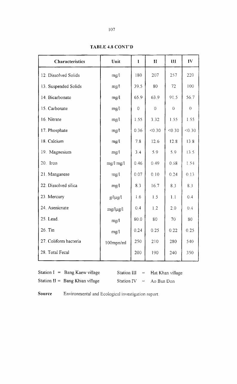
107

TABLE 4.8 CONT'D

Characteristics

12. Dissolved Solids

13. Suspended Solids

14. Bicarbonate

15. Carbonate

16. Nitrate

17. Phosphate

18. Calcium

19. Magnesium

20. Iron

21. Manganese

22. Dissolved silica

23. Mercury

24. Asenicnate

25. Lead.

26. Tin

27. Coliform bacteria

28. Total Fecal

Station I = Bang Kaew village

Station II = Bang Khian village

Unit I

mg/l 180

mg/l 39.5

mgll 65.9

mg/l 0

mg/l 1.55

mg/l 0.36

mg/I 7.8

mg/l 3.4

mg/I mg/l 0.46

mg/l 0.07

mg/l 8.3

g/l~g/l 1.6

mg/l~g/l 0.4

mg/l 80.0

mg/l 0.24

100mpnlml 250

200

Station 1lI

Station IV

n IJl

207 257

80 72

63.9 91.5

0 0

3.32 1.55

<0.30 <0.30

12.6 12.8

5.9 5.9

0.49 0.68

0.10 0.24

16.7 8.3

1.5 1.1

1.2 2.0

80 70

0.25 0.22

2]0 280

190 240

Hat Khan village

Aa Ban Don

Source Environmental and Ecological investigation report.

IV

220

100

56.7

0

1.55

<0.30

13 8

13.5

1.54

0.13

8 ' .J

OA

OA

80

0.25

540

350

108

TABLE 4.9

WATER QUALITY IN THE RESERVOIR AND PI-rUM OUANG RIVER

POST -IMPLEMENTATION

Characteristics Unit I n In

1. Temperature QC QC

Air 28.2 29.6 29.4

Water 27.9 28.9 29.1

2. pH, Units 606 6.9 7.0

'"' DO mg/l 5.8 7.0 72 -'.

4. Salinity ppt - - -

5. Conductivity u mho/cm 186 82 76

6. BOD mg/l '"' ') -'.- 2.5 5.8

7. SS rng/l 134.5 98.0 72.0

8 TS mg/l 312.4 132 120

9. Total Alkalinity as CaC03 mg/l 24.7 26.4 26.2

10. Total Hardness, as CaC03 rug/I 42.2 41 39.4

11. Chloride rug/! 8.8 .58.7 6.6

12. Phosphate mg/l 0.16 0.24 0.29

13. Nitrate mg/I 1.8 - 0.12

14. Sulphate mg/I 5.7 12.9 15.2

IV

29.0

28.8

7.2

7.5

1.0

310

9.5

1926

356.2

54.l

46.8

6.7

030

0.26

18.6

109

TABLE 4.9 CONT'D

Characteristics Unit

15. Ca mg/I

16. Mg mg/l

17. Mn mg/l

18. Fe (total) mg/l

19. Fecal Coliform Bacteria mpnil00

20. As

21. Cd

22. Pb

23. Hg

24.Zn

25. Pesticide

Station I

Station II

Source

Bang Kaew village

Bang Khian village

Survey data

rnl

rng/l

mg/l

mg/I

mg/l

rng/l

I

8.9

4.6

0.08

0.55

340

<0.005

<0.003

<0.002

<0.001

<0.003

0.085

Station III

Station IV

n If I

6.5 6.2

lA 1.1

0.01 0.02

0.18 1.8

240 360

<0.005 <0.01

<0.003 <0.002

<0.002 <0002

<0.001 <0.001

<0.003 <0.003

0.084 0.096

Hat Khan village

Ao Ban Don

IV

5.8

1.15

0.01

0.8

720

<0.008

<0.003

<0003

<0.001

<0003

0.094

110

5. SOIL AND LAND CAPABILITY

5.1 Introduction

A soil property (S) is dependent upon, or is Cl function of, the soil-forming

factors, i.e., Climate (Cl), organisms (0), relief (R), parent material (P), and time (T).

These can be presented in a form of an equation.

S f(CI, 0, R, P, T)

This implies that it is possible to take any soil-forming factor and consider its

variations against the background of the others, thus examining effect of that particular

one. However, in studying change in soil of an area, micro-environment of the area, even a

small one, may vary considerably. This variation inevitably renders considerable

heterogeneity of soil in the area. Effects of micro-environment on soil are thus, to a large

extent, masked by variation in micro-environment. Accordingly, to be obserable the effects

of micro-environment must be large enough to outrun soil heterogeneity, This means that a

soil-forming factor should play its role for a long time, probably not less than a fe\v

decades, before its effect on soil is observable, unless effect of soil heterogeneity is

overcome.

Land capability clssification is based on properties of soil, topography, erosion,

drainage, productivity and environmet of the land. Among these, drainage is practically the

only factor that may be changed by the implementation of Rajjaprabha project to an extent

that land capability is, in turn, affected by the change. This is mainly through change in

uderground water level as a result of irrigation and drainage facilities development, water

resource management enchanced by the project.

5.2 Objective and Scope

The mam objective of the study on soil and land capability is to evaluate

changes in soil and/or land capability after the implementation of the project. In addition,

information on soil and land capability of the project area available to date has also been

reviewed.

5.3 Methodology

To attain the objectives, the followings are undertaken.

(a) Review and compilation of data on soil, land capability recorded before

and after the implementation of the project.

Cb) Comparisons of water table levels obtain from the present study with tho se

obtained in the pre-impoundment study.

(c) Evaluation of the effect of changes in water table levels found in (b) on

soil and land capability.

C d) Conduct a field reconnaissance survey in the project area to :

(1) Evaluate general soil fertility of different areas by observing growth

and visual symptoms of vegetation and/or crops, soil characteristics,

topography, and interviewing.

(2) Observe soil cultural practices adopted by the farmers.

(3) Study characteristics of the irrigation system and its progress of

development.

5.4 Results of the Study

Soils in the upstream area are mainly of red-yellow Podzolic group derived

from shale, granite, quartzite and limestone. Lateritic nodules are scattered in the area.

Root penetration and horizon of parent material are rather deep, about 68 cm in depth

Physical and chemical properties of the soils at various elevations vary only slightly \Io,:ith

type of land use, elevation, and soil depth. The surface soils range from non-erosive to

slightly erosive. Soils covered by tropical rain forest are more stable than those found in

rubber plantations and agroculture area. Fertility of the soils range from low to moderate

levels. Phosphorus is presumably the most serious limiting factor in most soils. Due to

steep slopes and heavy rainfall land capabilities of most soils in the upstream area are

limited by high risks of soil damage.

The areas on the soil map are map units, developed during the survey on the

basis of soil classification, which followed that of the U.S.D.A. Soil Texonomy. The

lowest category of soil classification used here is soil series. In total, 16 map units were

distinguished in the project area. They consist of 5 soil series, 2 soil variants, 7 soil

associations and 2 miscellaneous land types. The list of these mapping units and area

covered by individual units is present in Table 4.10.

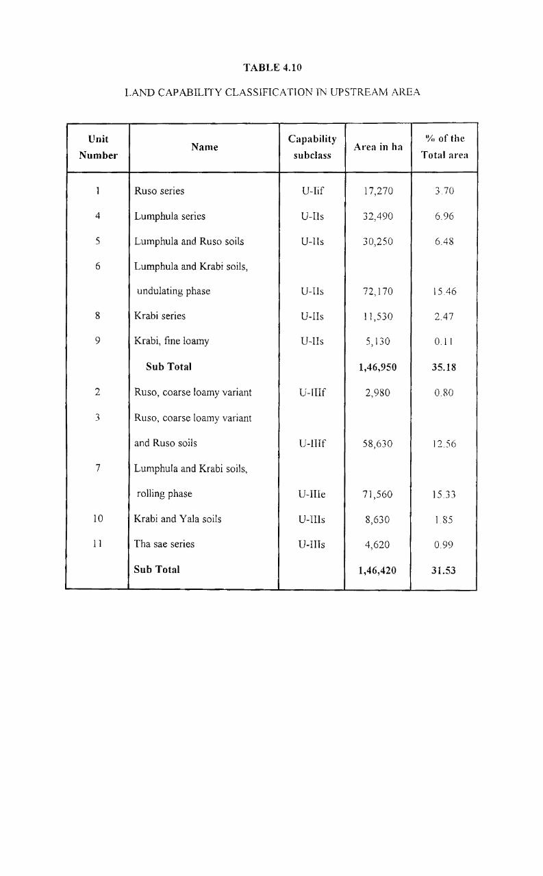
TABLE 4.10

LAND CAPABILITY CLASSIFICATION rN UPSTREAM AREA

Unit Capability 'Yrl of the Name Area in ha

Number subclass Total area

1 Ruso series U-lif 17,270 3.70

4 Lumphula series U-Ils 32,490 6.96

5 Lumphula and Rusa soils U-lls 30,250 6.48

6 Lumphula and Krabi soils,

undulating phase U-Us 72,170 15.46

8 Krabi series U-lIs 11,530 2.47

9 Krabi, fine loamy U-lIs 5,130 0.11

Sub Total 1,46,950 35.18

2 Ruso, coarse loamy variant U-IIIf 2,980 0.80

3 Rusa, coarse loamy variant

and Ruso soils U-lIIf 58,630 12.56

7 Lumphula and Krabi soils,

rolling phase U-IIle 71,560 15.33

10 Krabi and Yala soils U-Ills 8,630 1.85

1 ] Tha sae series U-Ills 4,620 0.99

Sub Total 1,46,420 31.53

114

TABLE 4.10 CONT'D

Capability (1<, of the Total Unit Number Name An'a in a

suhclass area

14 Khlong Teng and Na

Thon soils U-IVs 10,550 2.26

12 Yala series U-IVs 1,910 041

13 Yala and Lumphula soils U-IVs 2,800 0.60

Sub Total 15,260 ]3.27

16 Slope complexes, shale, U-VIIe 119,540 25.61

15 Slope Complexes, U-VIUe 8,990 1.82

limestone Water - 12,090 2.59

Sub Total 140,120 30.02

Grand Total 466,800 100

Source Department of Land Development, Ministry of Agriculture.

In the downstream area detailed reconnaissance soil maps covering the project

area in Surat Thani have been published by the Department of Land Development Most oC

the soils in Surat Thani province are reported to have low fertility. Soil survey and

classification were also carried out for the Phase 1 irrigation area during its feasibility

study to a semi-detailed level of investigation. Soils in the project area were classified into

6 classes based on their limitation in use for growing upland crops and low land rice. Three

in 6 classes were considered as irrigable and suitable for cropping.

115

C01\Cerning potential land use or land capability, all land in the upstre(]111 area

is practically unsuited for commercial crops, but suited for woodland or for establishment

of watershed protective vegetation. There are two major land types in the downstream area

One type is well suited for wet land rice in the rainy season. And with irrigation it can be

used for multiple cropping of rice, vegetables, and other crops. The other land type IS

wellsuited for many kinds of fruit trees, beverage crops, industrial oil crops, and rubber.

The lands were classified for both rice and upland crop suitability, with

subscripts showing their limitation; namely s-for soil deficiency, t-for topographic

limitation, d-drainage deficiency, a-salinity hazard, f-annual flooding, and c-vegetation

cover.

The results of the land survey (Royal Irrigation Department, \996) are

presented in Table 4.11 and are summarized as follows:

Area, (ha) O/., of total

(1) Lands suitable for irrigated rice 16,560 72

(2) Lands equally suitable for irrigated rice

and uplands crops 2,850 12

(3) Lands suitable for irrigated

uplands crops 2,310 10

Sub total irrigable lands 21,720 94

(4) Non irrigable lands 1,380 6

Total 23,100 100

116

TABLE 4.11

LAND CLASSIFICATION IN PHASE llRRlGAT10N PROJECT AREA

Arca, Arca, (~, of

Land Classification Sun'eyed (ha) (ha)

Lands

Land suited for rice 16,560 72

RI class 9,310

U2sIR1 2,922

U2s1R1.c 1,591

U3s/R1 1,667

U3slR1.c 384

U3sd/R1 2,746

R2 class 5,010 22

U3clR2.c 474

U3sdlR2d.f 4,111

U6sd/R2sd.f 339

U6sd/R2sd.fc 86

R3 class 2,240 10

U3sdlR3sd.f 214

U6sdfR3d.f 22

U6sd!R3sd.f 157

U6sd/R3sd.af 940

U6sdIR3 sd. afcl 907

L"nd~ ~!luall;): ulit~d for ri~!i: and Jlp1and

CrQD~ 2,850 12

U21R2 class 2850

U2slR2.c 580

U2slR2.d 35

U2s!R2s 732

U2slR2s.d 73

U2s/R2s.~ 1,430

TABLE 4.11 CONT'D

Land Classification Area~ Area, ·XI of Surveyed

(ha) (ha) Lands

Land~ ~llit~d fQr llu1and ~qm~ 2,310 1Q

UI class 690 3

UIlR2s 46

UIlR2s.d 34

UIIR3s 335

UI1R3s.d 69

UI1R3s.c 206

U2 class 1.510 7

U21R3s.d 140

U21R3s.c 1,120

U2sIR3s 139

U2slR3s.c 67

U2st/R3 s1. d 44

U3 class llQ

U3stlR6st.d 83

U3 stlR6st. c 27

Sub-total, irrigable lands 21,720 94

Non Irrigable Lands 1,380 1,380 Q

Class 6 925 -

6B 455 4

Other class 6 2

Total, surveyed lands 23,100 100

Sources Royal Irrigation Department.

118

In the pre-impoundment soil survey in the Phase 1 irrigation area large

fluctuations of ground water table was found throughout the year, with peak levels within

50 cm depth. Significant changes in the maximum levels of the ground water table would

affect land capability, as the high levels would provide suitable conditions for the water

logging problem. The observations of the ground water table in this post-impoundment

study, however, reveal no significant change. Therefore capability of the land in the

irrigation area has thus far not been significantly affected by the Rajjaprabha dam and its

downstream project implementation.

3.5 Conclusion

Most soils in the project area are generally of low to moderate fertility

Practically all soils in the upstream area are not suited for commercial crops due to steep

slopes.

The downstream areas are well suited for cropping, though generally requiire

appropriate management. Soil improvement, especially in fertility, is needed for crop

production in the project area.

Land capability of the project area has so far not been significatly affected by

the implementation of the project.

119

6. MINERAL RESOURCES

6.1 Introduction

The pre-impoundment investigation in the year 1980 indicated that there were

very scarce mineral deposites in the reservoir area, and there was no mine in operation in

the upper catchment area. Even though the mineral resource development in the basin is

not as active as in other parts of the south, the availability of mineral resources which have

been investigated by the Department of Mineral Resources have shown considerable

potential for development. The study on mineral resources is aimed at the assessment of

mineral resources development potential and its relative impacts, in order that its proper

development and mitigation can be integrated in the plan.

6.2 Objective

The objectives of this study are:

(a) To evaluate the potential for mineral resources development due to

improved access to watershed areas and availability of electric power.

(b) To assess the anticipated impacts of mining activities on surface water

quality in the upper and lower catchments area.

6.3 Methodology of the study

The methodology adopted for this study are:

(1) Collecting information on mining locations, mining processes, production

statistics, and development potential for each kind of mineral.

120

(2) Field survey and water sampling for selected mines in the upper and lower

catchments area.

(3) Evaluation of the impacts of mining activities on surface water quality in

collaboration with the water quality study task.

6.4 Results off the Study

In the pre-impoundment environmental and ecological study in 1980 it was

concluded that dolomite and kaolin deposits in the Phum Duang basin area were few

uneconomical for mining regardless of other unfavorable circumstances there. However,

after about a decade mining activities have not significantly developed. In this post­

impoundment study a total of 12 concessions, same as the reported in 1980, covering a

total area of about 164.6 ha is in operation (Table 4.12 and 4.13). Most of them are

dolomite mines, and located mostly in Khirirattha Nikhom district of Surat Thani province.

Mineral production in this area during January-April 1996 were 18,390 tons of dolomite

and 1,600 tons of kaolin, of about 6.43 and 0.616 million bhat repectively (Table 4.14),

however, production rate is very small compared to those produced in other areas of the

south (less than 1 percent).

The minerals already mined in this area are assessed to be of only small

portion of the area having mineral reserves. Hence, potential for minings in the area will

remain for a considerable period of time. Under the current mining practices, the

environmental impact from mmmg operation in the Phum Duang river basin is under

control. As required by the governmental regulation, the environmental impact from

mining on land, water, ecology, transportation, socio-economics, and public health must be

mitigated in the operation. The investigation on water quality has indicated that the

operating mines in the area have not caused any serious problem on surface water quality

as most of the mining an open pit mines and they do not use water in the processes.

TABLE 4.12

PREVIOUS MINING CONCESSIONS IN WATERSHED AREA

Concession, No. A.·ea, ha Holders

1. 1012504 15.2 Easter Mining Development Co. Ltd.

2. 24/2504 15.8 Easter Mining Development Co. Ltd.

3. 2512504 15.6 Easter Mining Development Co. Ltd.

4. 26/2504 15.4 Easter Mining Development Co. Ltd.

5. 46/2505 13.6 Easter Mining Development Co. Ltd.

6. 19/2512 42.4 Easter Mining Development Co. Ltd.

7. 26/2520 15.4 Easter Mining Development Co. Ltd.

8. 2712520 34.1 Easter Mining Development Co. Ltd.

9. 50/2520 9.5 Rae Samphan Co. Ltd.

10. 6412522 43.2 Rae Samphan Co. Ltd.

11. 65/2522 43.2 Rae Samphan Co. Ltd.

12. 6612522 32.0 Rae Samphan Co. Ltd.

Total 292.2

Source Department of Mineral Resources

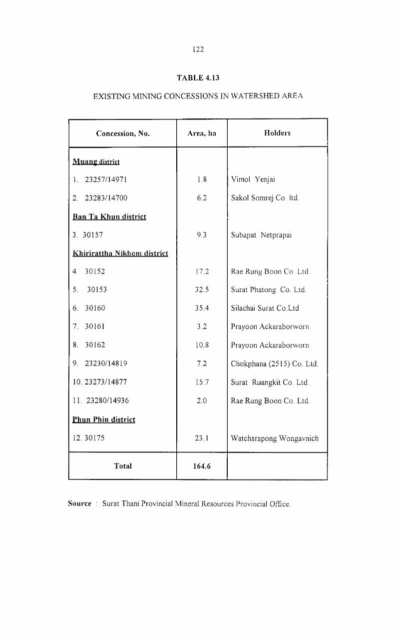
122

TABLE 4.13

EXISTING MINING CONCESSIONS IN WATERSHED AREA

Concession, No. Area, ha Holders

Muang district

1. 23257114971 1.8 Vimol Yenjai

2. 23283114700 6.2 Sako! Somrej Co. ltd.

Ban Ta Khun district

3. 30157 9.3 Subapat Netprapai

Kh irirattha N ikhom district

4 30152 17.2 Rae Rung Boon Co Ltd.

5. 30153 32.5 Surat Phatong Co. Ltd.

6. 30160 35.4 Si!achai Surat Co. Ltd

7. 30161 3.2 Prayoon Ackaraborworn

8. 30162 10.8 Prayoon Ackaraborworn

9. 232301I 4819 7.2 Chokphana (2515) Co. Ltd.

10. 232731I4877 15.7 Surat Ruangkit Co. Ltd.

11. 23280114936 2.0 Rae Rung Boon Co. Ltd.

Phun Phin district

12. 30175 23.1 Watcharapong Wongavnich

Total 164.6

Source Surat Thani Provincial Mineral Resources Provincial Office

123

TABLE 4.14

MINES PRODUCTION IN THE WATERSHED AREA

(JANUARY-APRIL 1996)

Unit: in baht

Location Mines Tons Values (Bath)

Khirirattha Nikhom district Dolomite 18,390 6,436,500

Muang district Kaolin 1,600 6,16,000

Total 7,052,500

Source Surat Thani Provincial Office.

124

7. EROSION AND SEDIMENTATION

7.1 Introduction

Generally, erosIOn and sedimentation are considered impor1ant cause of

problems in regard to the operation of most dam and reservoir projects. The effects of gredt

concern are sedimentation deposition in the reservoir and riverbank erosion downstream of

the dam. The construction of Rajjaprabha will cause the significant change of the natural

regime of the Khlong Saeng and, later, Phum Duang river.

Farther downstream to the river estuary where the river discharges to the sea,

the carried sediments will settle because of the reduction in flow velocity. Deltas will be

formed and that will obstruct navigation. With the presence of the dam there will be

change in sediment load and river discharge which will lead to change in estuarine

sedimentation process. The impacts as mentioned above are no exception to Rajjaprabha

dam. Expect trends and magitudes of these inpacts are evaluated in this study.

7.2 Areas of Study

Since the impacts of the dam on various portions of the river arc different in

nature, the study is separated into three different areas as follows:

(a) River bank erosion.

(b) Sedimentation in reservoir.

(c) Estuarine sedimentation.

125

7.3 Results of the Study

7.3.1 Previous Study

The annual suspended sediment, expected to be discharged into the proposed

Rajjaprabha reservoir was estimated by EGAT (1979) using the correlation of annual

runoff. The ratio of mean annual runoff between Khlong Saeng at damsite and PhuJ11

Duang river is about 67.60 percent. Consequently the average suspended flowing into the

reservoir would be 3,36,603 tons/year. This amount is quite close to obtained from the

analysis of the National Energy Administration (NE A) records. The bed load of sediment

transported into the reservoir was estimested by EGAT from the annual suspended load.

The annual bed load was assumed to be about 20 percent of the annual suspended load as

found from the Pattani multipurpose project (EGA T.1976). The total annual sediment load

discharging into the proposed reservoir is as follow.

Annual suspended sediment load

Annual bed load = 0.20 x 3,36,603

The total annual load of sedimentation

3,36,603

67,321

4,03,924

tons

tons

tons

By assummg the unit weight of 1.303 tons/m3, the total sediment load of

4,03,924 tons comes to 3,09,995 m3 The corresponding depth of watershed erosion is 022

millimeters per year. This rate of watershed erosion is raher high in comparison with other

regions in Thailand but is low as compared with the watershed in other contries, as shown

in Table 4.15.

126

TABLE 4.15

ANNUAL DEPTHS OF EROSION IN VARIOUS WATERSHEDS

Annual Depth of River basin Country

Erosion mm/yea!"

1. Domodar India 095

2. Ching (Yellow) China 4.86

3. Yantze China 0.35

4. Mekong lndochina 0.10

5. Irrawadi Burma 0.55

6. Ping (at Bhumibhol dam) NOJ1hern Thailand 0.36

7. Wang Northern Thailand 021

8. Yom Northern Thailand 0,21

9. Nan Northern Thailand 0.23

10, Upper Ping Northern Thailand 0.2!

11, Nam Pong Northeastern Thailand 0.13

12. Chao Phraya Centralthern Thailand 0.14

13. Pattani Southern Thailand 0.189

14. Khlong Saeng * Southern Thailand 0.22

Source: EGAT

* Estimated previously and listed herein for comparison

127

7.3.2 River Bank Erosion

River bank erosion is relatively not serious for the river reach further upstream

from Ban Ta Khun district that was found to be of 97,199 tons. More severe erosions are

found along Khlong Phum Duang downstream from the Rajjaprabha diversion dam, which

is an artificial reach cut long time ago. Bank erosion in this downstream river reach f1'ol1l

the diversion dam is still very active. The bank erosion should have decreasing trend since

downstream flood potential is minimized by the Rajjaprapha reservoir regulation.

River bed degradation has been assessed from field investigation and frol11

available cross section data. No serious bed degradation at anticipated locations

downstream from the Rajjaprapha dam is evidenced.

7.3.3 Sedimentation in the Reselvoir

Sedimentation in the Rajjaaprabha reservoir is found to have negligible etfect

on the useful functions of the reservoir as originally planned. Although lack oC actual

reservoir sedimentation survey data, possible effects of increased sediment load from

headwater areas of the reservoir are assessed. The post-impoundment which was surveyed

by EGA T in 1995 found the sediment load at about 3,74,000 tons per year \\lhich should 20

percent increase from the pre-impoundment data. About 20 percent increase in sediment

load reservoir sedimentation is recalculated using the Area-Increment Method. It is found

that even with the 20 percent increase in the reservoir sediment load most of the

conclusions drawn in the reservoir sedimentation aspect in the pre-impoundment study are

still valid. And the Rajjaprabha reservoir should be capable of providing its beneficial

functions for more than 7,000 years of service life (Table 4.16).

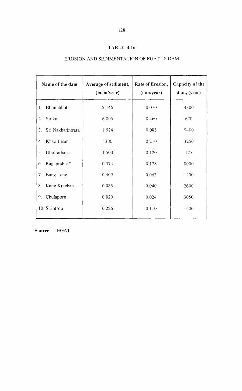
128

TABLE 4.16

EROSION AND SEDlMENTA nON OF EGAT ) S DAM

Name of the dam A verage of sediment, Rate of Erosion, Capacity of the

(mcm/year) (nun/year) dam, (year)

1. Bhumibhol 2.146 0.070 4300

2. Sirikit 6.006 0.460 670

.., Sri Nakharintrara 1.524 0.088 9400 -'.

4. Khao Learn 1300 0.210 3250

5. Ubolrathana 1.500 0.120 125

6. Rajj aprab ha * 0.374 o 178 8000

7. Bang Lang 0.409 0.063 1400

8. Kang Krachan 0.085 0.040 2600

9. Chulaporn 0.020 0.024 3050

10. Sirintron 0.226 0.110 1400

Source EGAT

129

7.3.4 Estuarine Sedimentation

As concerns estuarine sedimentation, the present reduction in the sediment load

In the Ao Ban Don estuary due to the presence of the storage and diversion dams IS

estimated to be rather slight, not more than 15 % reduction from those experienced prior

to the dams construction. The slight effect can be explained from the fact that more

sediment loads are picked up from the river banks and beds as tbe relatively clear water,

with unsatisfied sediment carrying capacity, traverses the downstream river reach before

reaching the estuary. These phenomenons of sediment load picking up downstream from

the dams were evidenced during both sets of sediment concentration sampling along the

whole river reach. The amount of dredged motional from Ao Ban Don estuary is shc)\vn in

the Table 4.17.

130

TABLE 4.17

CHANNEL IMPROVEMENT IN AO BAN DON ESTUARY 8Y DREDGING

Year Month Amount of Or-edged

motio Ilal (m3)

October 1989 64,39 I

November 1990 1,95,280

December 1991 2,01,906

January 1992 1,57,290

February 1993 1,16,138

March 1994 1,88,144

April 1995 81,145

May 1996 57,810

Total 10,62,415

Source From the Harbour Department

131

8. SALINITY INTRUSION

8.1 Introduction

Salinity intrusion into the river is a natural phenomenon inl1uenced mainly by'

the amount of fresh water flow into the estuary and the tidal condition prevailing at the

river mounth. Salinity of the water in the estuarine reach varies ,",,,ith the location from tile

river rnounth, being less saline at locations far upstream cfrom the river mounth At a

location in the estuarine river reach the salinity also ditfers at different depths, being more

saline at the deeper depths due to the higher specific gravity of the salt water. The variation

of salinity both with the distance from the river mouth and with the river depth is also time

dependdent, following the time variatin of the fresh water intlow and the tidal variation

Therefore, under natural conditions the salinity distribution pattern in the estuary

continually moves back and forth along the river, with its vertical salinity gradient also

varying as the mixing of different layers of water continues

In this study salinity intrusion is investigated to serve as basic information for

other related studies.

8.2 Objectives

The objectives of salinity intrusion study are:

(1) To present the salinity intrusion pattern in the Phum Duang estuary.

(2) To establish relations among fresh water inflow, salinity, and distance

from the river mouth.

132

8.3 Salinity Data Collection

The sampling locations of the measurement were about 500 111 apart, from the

river mounth to about 5 km upstream. Samples were taken from the bottom, mid-depth,

and water surface along the river thalweg. The Salinity data are classified into two sets.

The first set consists of the measurement during the rising tides, and the second set consists

of the measurement made shortly after high water slacks. The rising tide data include the

measurements on 6th march, and 20th July] 997. And the high water slack data consists of

the measurements on 25th August, and loth September 1997. River flows measured at the

Phun Phin bridge during the days with salinity measurement.

8.4 Results of the Study

8.4. t Salinity Distribution Pattern

Pattern of salinity distribution in the Phum Duang eatuary are illustrated by line

of equal salinity concentration, referred to as haloc1ines. During the rising tides the

haloc1ines slanted sharply resembling a wedge intruding under the freshwater. The saline

water and fresh water partially mixed during these rising tides. The mixing became more

effective during the high water slacks when the haloclines were observed to be closer to

vertical position. The salinity intrusion patterns observed in these measurements varied

from the partially mixed to well mixed type. The maximum intrusion (I ppt salinity) found

in these measurements was less than 2.5 km from the river mouth.

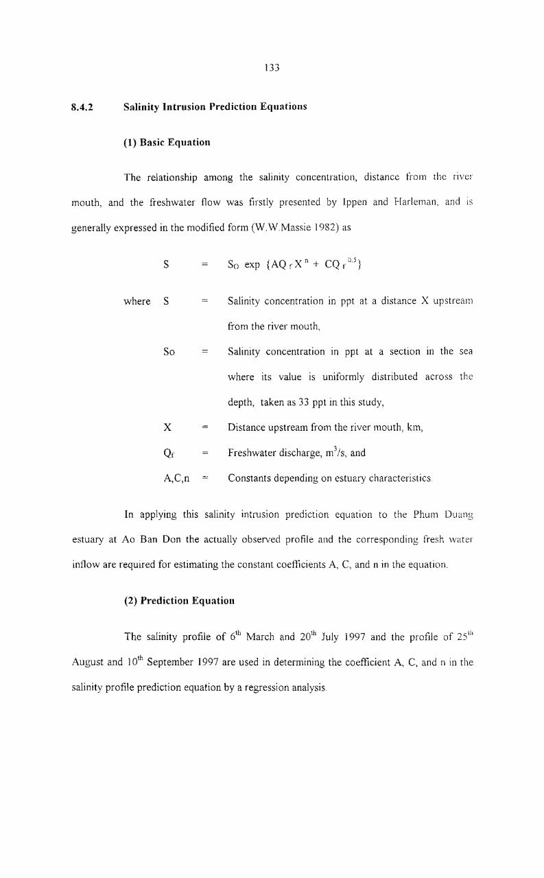
133

8.4.2 Salinity Intrusion Prediction Equations

(1) Basic Equation

The relationship among the salinity concentration, distance from the river

mouth, and the freshwater flow was firstly presented by Ippen and Harleman, and IS

generally expressed in the modified form (W.W.Massie 1982) as

S

where S

So

X

Qr

A,C,n

So exp {AQ f X n + CQ flU}

Salinity concentration in ppt at a distance X upstream

from the river mouth,

Salinity concentration In ppt at a section 111 the sea

where its value is uniformly distributed across the

depth, taken as 33 ppt in this study,

Distance upstream from the river mouth, km,

Freshwater discharge, m3/s, and

Constants depending on estuary characteristics.

In applying this salinity intrusion prediction equation to the Phum Duang

estuary at Ao Ban Don the actually observed profile and the corresponding fresh water

inflow are required for estimating the constant coetIicients A, C, and n in the equation.

(2) Prediction Equation

The salinity profile of 6th March and 20th July 1997 and the profile of 25 th

August and 10th September 1997 are used in determining the coefficient A, C, and n in the

salinity profile prediction equation by a regression analysis.

134

For the high water slack condition the prediction equation is

S 33.0 exp {- 0.0658 QrX \.65 _ 0.076 Q 1°5 }

And for the rising tide condition the prediction quation is

S = 33.0 exp {- 0.0384 Qf:o.26 - 0.136 Qros }

The two prediction equations are verified by USIng them in fitting salinitv

concentration profiles to the data measured during different periods, by Llsing trial values

of fresh water inflow where the actual flows were unknown.

8.5 Conclusion

Salinity intrusion patterns observed in the Phum Duang estuary in this study

are of partially mixed and well mixed types. The maximum intrusion of 2.5 ppt salinity

was observed during the field measurements at less than 2.5 km upstream from the river

mouth. Even the 0.5 ppt salinity intrusion was observed to be less than 5 km from the river

mouth. Results of field measurements of salinity data and their concurrent fresh water

inflow into the estuary have been used to establish useful salinity intrusion prediction

equations. Salinity concentration at certain location along the river mouth can now be

predicted for different fresh water flows in the estuary.

CHAPTER V

ECOLOGICAL RESOURCES

CHAPTER V

ECOLOGICAL RESOURCES

1. INTRODUCTION

In general, the major components of ecological resources relating to a

dam/reservoir development project include aquatic biology, fisheries, forests, wildlife, and

reservoir ecology. These environmental resources will be affected directly by dam

construction and reservoir formation. With respect to fisheries, the effects will be both

benefits and losses, depending upon what location along the river stretches they arc

considered. As for forests and wildlife, the effects are ususlly adverse. Fisheries, aquatic

biology, and reservoir ecology are closely related to one another because changes in

conditions of any parameter will have impact on the other two parameters Likewise.

forests and wildlife have very close relationships to each other. Thus, in this study, the

ecological resources will be presented in four main parts: (i) aquatic ecology and aquatic

weeds (ii) fisheries (iii) forestry and (iv) wildlife.

2. AQUATIC ECOLOGY AND AQUATIC WEED

2.1 Introduction

Ecologically speaking, any attemt to change land use patterns bring about

changes in environment, both in natural flora and fauna. Thus the construction of a dam

and a reservoir will naturally affect biological processes in the area. When the habitat

changes, many fauna will also change to adapt themselves to survive.

136

Investigation and assessment including forecasting probable effects on this

aspect were made in the environmental and ecological investigations. At this early stage of

impoundment it is very crucial that actual effects be observed and compared with thos(:;

anticipated so that necessary mitigation measures, if any, can be timely made. Special

consideration is given to aquatic ecology aspects of food sources, which in turn, atTect

tisheries productivity

2.2 Objectives

Main objectives are to evaluate the reservoir and downstream area in terms of

aquatic ecology after 10 years operation of the dam These include studies of plankton and

benthic animals, which represent indicators of the water's productivity. The aim of the

study is to gain information on species diversity, species richness and evenness, biomass,

and community, including their seasonal variations in both wet and dry seasons. The study

results are then compared with the previous study to assess changes, and subsequently

utilize for preparing recommendations to enchance beneficial changes.

The specific objectives may be summarized as follows:

(a) To investigate aquqtic ecology and aquatic weeds III the reservoir and

downstream river.

(b) To evaluate species diversity, richness and evenness, biomass community,

and their seasonal variation.

(c) To compare the results to the previous study.

2.3 Study Area and Duration

Two fIeld investigations were conducted to coHect specimens at 6 stations Of

these stations two are in the reservoir and four along the Phum Duang river (see Figure :'i. I)

The first field investigation was performed in order to collect data to represent dry season

conditions, and was conducted during 1-7 April 1997. The second field investigation was

performed to collect data for the wet season, and conducted during 15-20 November 1997.

2.4 Methods of Study

The methods used for biotic investigation are as follows.

(1) Benthos

(1. 1) Peterson and Ekman Dredges were used to collect soil samples, the

contents were sifted with the US standard Sieve No.30. Benthic animals

left on sieve were preserved in 5 percent formalin identified, weighed,

and counted to calculate the abundance per square meter of the benthos

and biomass at each sampling point

(1.2) Calculations were made to find the Species Diversity Index of benthic

animals, which clearly shows the relationship between the species and

numbers of animals in that particular point, using Shanon-Weiner Index.

(2) Plankton

(2.1) Clarks Modification of Juday plankton trap was used to collect

plankton at 1 meter water depth in the river, and in the reservoir at I

and 10 meter depths.

[ 38

(2.2) The collected samples were preserved in 5 percent formalin for

subsequent identification and number determination.

(2.3) Calculations were made to find the Species Diversity Index, using

Margalef or Shanon-weiner Diversity.

(3) Aquatic Weeds

The aquatic weeds were observed both in the reservoir and dovmstream at the

same station as for benthos and Plankton study. Plant specimens were collected according

to the plant types as follows:

(31) The marginal type plants were found in the swamp area around the edge

of the reservoir and along both edges of the riverbanks. The plant

specImens were collected and preserved in herbarium for further

identification.

(3 2) The water body type plants consisted of floating specl cs, submerged

specIes and emergent sepcles. Some specimens were dry-preserved and

particular plant were preserved 111 5 percent formalin or 50 percent

alcohol.

2.5 Results of the Study

2.5.1 Animals

(1) Density

The benthic animals specllnens collected during the 2 field trips can be

classified into 7 groups Oligochaetes, dragonfly larvae, caddistly larvae, mayfly larvae,

139

midges larvae, univalves and bivalves. Populations of benthic animals found \vere not

uniform, depending on various factors such as nature of river bed, water currents, etc. The

findings are follows:

(1 .1) It was found that the bottom of the reservoir was covered with mud and

decayed plants. The number of benthic animals found during the dry season ranged from

18 per m2 (at station No.2) to 678 per m2 (at station No.l) with 367 per m2

on an average

During the wet season, the number ranged from 15 per m2 (at station No.2) to 224 per m2

(at station No.1) with 118 per m2 on an average.

(1.2) Between the storage and lower reach, the river bed was mostly covered

with mud, sand and gravel, and the water current was strong, except in the upstream from

the diversion dam where the river bed was covered with muddy sediments and water

moved sluggishly. The number of benthic animals in dry season ranged from 194 per me

(at station No.3) to 4,830 per m2 (at station No.4) with an average of 2,091 per 1112 During

the wet season the number ranged from 34 per 1112 (at station No.4) to 1,458 per rn 2 (at

station No.S) with an average of 636 per m2

(1.3) In the lower reach, the riverbed was covered with sandy soil and clay At

Station NO.6 at the river mouth the riverbed was very muddy. During the dry season, the

number of benthic animals raged from 16 per m2 (at station No.S) to 4,703 per m2 (at

station No.6) with an average of 2,029 per m2. During the wet season, the number ranged

from 32 per m2 (at station No.S) to 1,936 per m2 (at station No.6) with an average of 1,136

per m2

140

(2) Biomass of Benthic Animals

The biomass of benthic animals was calculated from the specimens collected

during the two field trips, these can be summarized as follows

(2.1) In the reservoir, the biomass of benthic animals was found during the dry

season ranged from 0.53 gm/m2 (at station No.2) to 163.5 gm/m2 (at station No.l) During

the wet season it ranged from 0.05 gm/m2 (at station N02) to 0.56 gm/m2 (at station No.1)

with 0.25 gm/m2 on an average.

(22) It was found that along the dam to lower reach, the biomass of benthic

animals in the dry season ranged from 1.85 gm/m2 (at station No.3) to 24.57 gm/m2 (at

station NoA) with an average of 2.15 gm/m2 During the wet season it ranged from 0.12

grn/m2 (at station No.3) to 30.68 gm/m2 (at station NoA) with 6.50 gmJm2 on an average.

(2.3) In the river reach the biomass of benthic animals during the dry season

ranged from 0.03 grnlm2 (at station No.5) to 240.5 gmJm2 (at station No.6) with an average

of 120.30 grnlm2 During the wet season it ranged from 0.95 gm/m2 (at station NoS) to

22.56 gm/m2 (at station No.6) with 11.2 gm/m2 on an average.

(3) Species Diver-sity Index

The study results can be summarized as follows.

(3.1) It was found that in the reservoir the species diversity index or benthlc

animals in dry season was 0.96 on an average while in wet season it was 0.34 on an average.

(3.2) Along the dam to the lower reach, the index numbers of benthic animals

during the dry season ranged between 0.12 (at station No.3) and 0.98 (at station NoA) with

141

0.62 on an average. During the wet season, the index numbers ranged from OJ (at station

No.3) and 1.2 (at station NoA) with 0.68 on an average.

(3.3) In the lower reach, the index number found during the dry season was

024 on an average, while during the wet season the number was 0.65 on an average

(4) Comparison of Benthic Animals before and after Impoundment

The data of the survey before and after the dam construction indicate similarity

111 the kinds of benthic animals. Apparently, the number of benthos in the reservoir was

lower after the construction. The average density of the benthos before the construction

was 786.6 per m2 while the average density of the benthos after the construction in dry and

wet seasons were 267.5 per m2 and 115.84 per m2, respectively.

The density of benthos in the downstream area was higher in the period after

the dam construction than in the period before the construction. The densities of the

benthos after the construction in dry and wet seasons were 3,128.2 per m2 and 243.78 per

m2 on an average respectively, while that of the period before the construction in dry

season was 124.6 per m2 on an average.

2.5.2 Plankton

(1) Density

The plankton specimens collected during the 2 field trips can be classified into

8 phyla, 78 genera. These consisted of 3 phyla 52 genera of phytoplankton, and 5 phyla 22

genera of zooplankton. The findings are as follows.

142

(1.1) It was found that in the reservoir the number of plankton during the dry

season ranged between 1,074 x 103 cells/m) (at Im depth) at station No.2 and 12,785 x 10·;

1 1 ·1 cells/m- (at 10 m depth) at station No.l, with 2,895 x 10 cells/nY an average

PhytopIankton found in abundance were Anacystis, Ceratium and Peridinium, while the

zooplankton was KerateIla_ During the wet season, the number ranged from 385 x 101

cells/m3 (at 10 m depth) at station No.2 to 3,885 x 103 cells/m3 (at I m depth) at station

No.1 with 1,885 x 103 cells/m3 on an average. The phytoplanktons found in abundance

were Anacystis, Cosmarium and Staurastrum while the zooplankton was Keratella

(1.2) Along the dam to lower reach, the number of plankton found during the

dry season raged from 185 x 103 cells/m3 (at station No_3) to 1,686 x 103 cells/ml (at

station NoA) with 685 x 103 cells/m3 on an average. The phytoplanktons found in

abundance was Anacystis_ During the wet season, the number ranged from 185)\ 1 0·'

cells/m" (at station No.3) to 885 x 103 cells/m] (at station NoA) with 315 x 10' cells/m"' on

an average The phytoplanktons found in abundace were An~ and Surirella.

(l J) It was found that in the lower reach, the number of plankton during the

dry season raged from 80 x 103 cells/m3 (at station No.5) to 155 x 103 cells/m) (at station

N06) with 80 x 103 cells/m3 on an average_ The phytoplanktons found in abundance \vas

A -D' h 1 1 nacystls, unng t e wet season, the number ranged from 85 x 10- cells/m- (at station

No.5) to 786 x 103 cells/m3 (at station No.6) with 365 x 103 cells/m3 on an average. The

phytoplanktons found in abundace were Thalassiosira.

(2) Species Diversity Index

The study results can be summarized as follows:

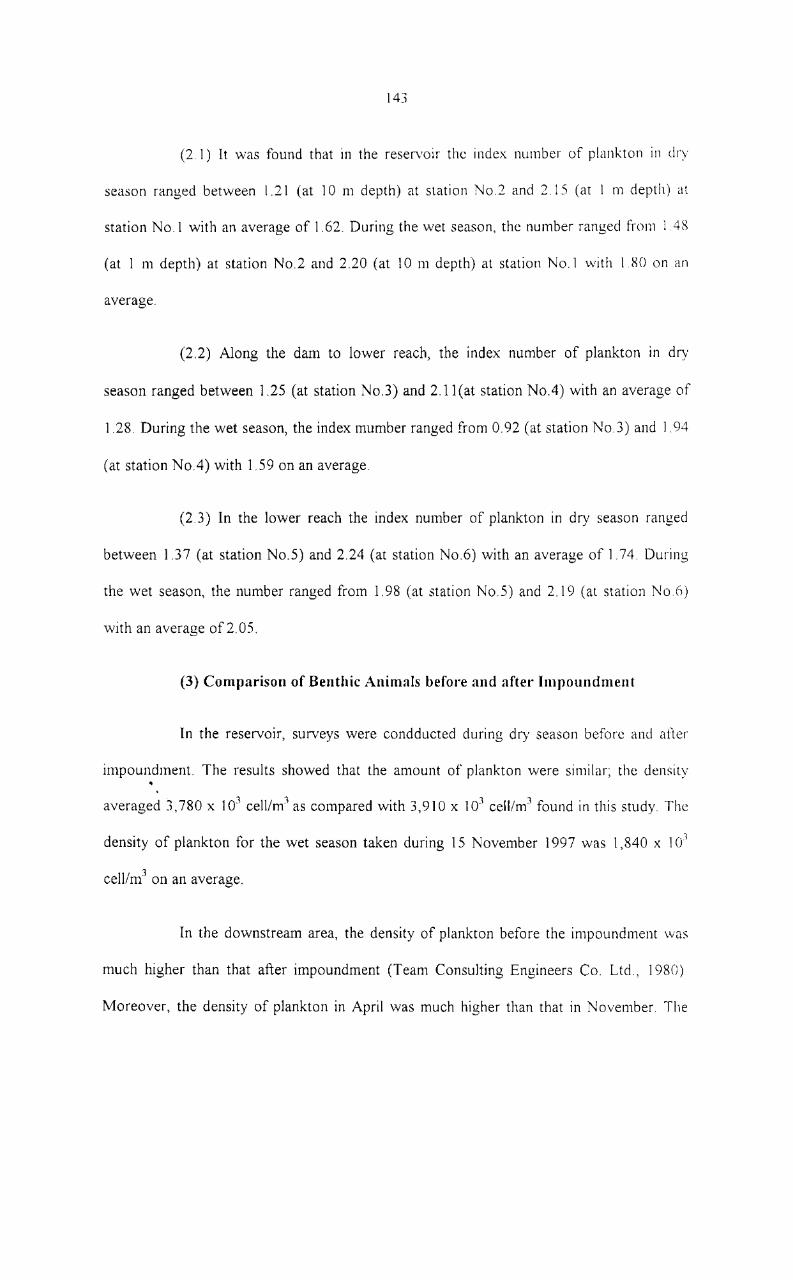
143

(2 I) It was found that in the reservoir the index number of plankton ill dry

season ranged between 1.21 (at 10 m depth) at station No.2 and 2.15 (at I m depth) at

station No.1 with an average of 1.62. During the wet season, the number ranged t1-<)11l 1 48

(at I m depth) at station No.2 and 2.20 (at 10 m depth) at station No.1 \vith I 80 on an

average.

(2.2) Along the dam to lower reach, the index number of plankton in dry

season ranged between l.25 (at station NoJ) and 2.11(at station No.4) with an average of

1.28. During the wet season, the index mumber ranged from 0.92 (at station N03) and J .94

(at station No.4) with 1.59 on an average.

(2.3) In the lower reach the index number of plankton in dry season ranged

between 1.37 (at station No.5) and 2.24 (at station No.6) with an average of 1.74. During

the wet season, the number ranged from 1. 98 (at station No 5) and 2. I 9 (at station No 6)

with an average of2.05.

(3) Comparison of Benthic Animals before and after Impoundment

In the reservoir, surveys were condducted during dry season before and after

impoundment. The results showed that the amount of plankton were similar; thc dcnsity •

averaged 3,780 x 103 cell/m) as compared with 3,910 x 10J cell/mJ found in this study The

density of plankton for the wet season taken during 15 November 1997 was 1,840 x 101

cell/m3 on an average.

In the downstream area, the density of plankton before the impoundment \vas

much higher than that after impoundment (Team Consulting Engineers Co. Ltd., 1980)

Moreover, the density of plankton in April was much higher than that in November. The

144

survey before impoundment was taken during 19-26 March 1980, while after

impoundment were taken in April and November 1997. The results showed the densities of

plankton for the two periods were 3,680 x 103 and 1,126 x 103 cell/m]

2.5.3 Aquatic Weed

Results from the first investigation revealed the existence of 41 species, :;:;

genera and 28 families of aquatic plants. These were marginal, submerged and floating

plants. Results from the second investigation indicated that the types of aquatic plants and

their numbers were slightly different from those of the first investigation. The number of

aquatic plants found at each sampling station can be summarised as follows

(1) In the reservoir, at all stations a small number of aquatic plants were found

This is due to the fact that when the inflow water was impounded in the reservoir the

higher level of water completely destroyed the original submerged plants grown in the

river. However, some new species of aquatic plants have appeared above the water level

along the edge of the reservoir.

(2) Along the lower reach of the dam (station No.3,4) the density by weight of

plants ranged between 567 gm/m2 (at station No.3) and 1,812 gm/m2 (at station 1'\0.4)

Aquatic plants found in abundance were Brachiaria Sp. And Hydrilla Sp.

(3) It was found that in the river reach, the density by weight was 2,512 gm/Ill"

(at station No.5) while at the river mouth no aquatic plant was found.

145

2.6 Conclusion

In the pre-impoundment environmental and ecological studies conducted 111

1980, biological conditions of the river were investigated at only 3 sampling stations onc

near the storage dam site, one at the upstream, and one at the downstream Thirty-t\vo

species of planktonic organisms were then observed, including 21 species of phytoplanklol1

and 11 species of zooplankton. The presence of plankton was reponed to be relatively high

as compared with the amount observed in other rivers in the country. Benthic organisms

were, however, found to be of low as the river botton: at the sampling sites was sane! and

gravel.

In this post-impoundment study, aquatic ecology has been investigated at 6

selected sampling stations; two stations in the reservoir and four stations along the river.

Field investigations were performed in both dry and wet seasons: during 1-7

April 1997 and during 15-20 November 1997, respectively. The amount of plankton in the

reservoir is not different from the amount found in the vicinity of the dam site in the pre­

impoundment period. Along the river between storage dam to the lower reach, the amount

of plankton is significantly less in the post-impoundment period. But, the benthic animals

in the post-impoundment period are more abundant. Both planktons and benthic animals

were more abundant during the dry season than during the wet season in the reservoir and

in the downstream river reach. Dowmstream from the diversion dam, planktons are less

abundant than in the upper river reach. Benthic animals in the vicinity of the river mouth

are more abundant.

146

Aquatic plants in the reservoir are scanty. They were more prevalent in the

river reach between the storage and diversion dam, and even more prevalent downstream

from the diversion dam. However, they were not found near the river mouth.

The aquatic ecology condition in the reservOIr reveals its suitability for

aquaculture development. This is also true for the downstream river reach, but perhaps to a

somewhat lesser extent.

147

3. FISHERIES

3.1 Introduction

Rajjaprabha reservoir is a man-made lake located in Surat Thani province, with

a water surface area of about 185 km2 or 18,500 ha. After the dam was built, the river's

ecosystem changed significantly. Some species of fish formerly living in the river adapted

themselves to survive in the new environment, while other species of fish could not

survive. They gradually disappeared and have been replaced by other species. This process

has had an impact on the fish population and the local people engaged in fishing.

The changes in the aquatic ecosystem due to the creation of the dam and

reservOir, the patterns and life cycles of riverine fauna including fish and

macroinvertebrate species are interrupted. Migration of the fishes to upstream of the dam is

not possible. The impoundment fisheries are affected by the changes in the water quality as

well as other physical changes in the reservoir. In most cases, after the impoundment, an

increase in the amount of reservoir fish is observed, and they represent a significant

economic asset of the projects. From the fishery point of view, it is important for proper

fishery management to conduct a study to assess changes, which have already occurred,

and to propose a proper management plan to enhance the reservoir fisheries development.

3.2 Objectives

The objectives of this study are as follows:

(1) To investigate the existing condition of fisheries' resources.

(2) To investigate the socio-economic condition of fishing households in the

project area; and

148

(3) To formulate an administrative plan and regulations for fisheries activities

in the reservoir and downstream, in order to enhance maximum sllstained

yield of fishes.

3.3 Study Methodology

The field work for the fisheries study originally consisted of two tleld

investigations, one in the dry season during 1-7 April 1997 and another in the wet season

during 15-20 November 1997. The fish sampling was obtained from four stations: two

from the reservoir, and another two stations from a downstream in Phum Duang river.

Data on fisheries activities and related socio-economic conditions of local

residents in the proposed reservoir area and downstream river reaches were gathered in a

fisheries socio-economic survey. The data was collected using a structured schedule, as

well as by inteviews with local fisheries officials. In the reservoir area, the samples

consisted of 100 households. They were selected on the basis of a simple random sampling

method. The sample size was about 26 percent of the total number of 385 households in

the resevoir area. In the downstream area a total of 80 sample households were selected

randomly, representing 10.5 percent of the total number of 762 households in the villages

In the delta area, interviewing a small number of fishermen carried out data gathering.

3.4 Previous Investigation

Information regarding fishery resources in the Phum Duang river basin during

pre-improundment was obtained from the environmental and ecological investigation

report. The information is summarized as follows.

149

3.4.1 Species composition

Ninety-three compositions of species were found. Among the number of species

found, cyprinids were ranked first (having 53 species abollt 66 percent) fl)llowed by catfish

(Il species or 11.8 percent), Conbitids (7 species or 7.5 percent), Mastacembelids 5 species

(5.4 percent), and miscellaneous fish with 17 species (about 18.3 percent). The fish species

were arbitrarily divided into "less common", "common" and "abundant". The proportions of

these categories were 7.5, 80.2 and 12.3 percent respectively. Of the 93 species found in the

reservoir and downstream, the "less common" species can be regarded as "rare" as far as the

Phum Duang basin, in concerned. But they cannot be considered as the "endangered" species

because they still exist in considerable quantities in other part. They include Pia Peap Khao

(oxygaster macuJeanda), Pia Peap Bai Phai Douronensis, Barb (Pantius coJemari), Mu (B.illi.a

Beauforti), and Katting Fai (Mastacembelus er:ythotaensis). Of the 93 species was found, 21

species (about 23 percent) were classified as the species of commercial values.

3.4.2 Major Fish Species and Standing Crop

Cyprinidae were family of fishes the most important, ones found in the area.

They constitute 96.89 percent of the total catch in term of number and 90.56 percent in

term of weight. On the other hand Pristolepicadae constituted 5.17 percent, Belonidae 2.18

percent, and Ohicephalidae 1.29 percent in term of weight.

The most prevalent species in the area was PIa Siew (Rasbora Rasbora

Hamilton), which constitute 58.94 percent in term of number and 27.73 percent in term of

weight. The other species included PIa Siew (Rasbora restrodorasalis HM.Smith), 18.61

pecent in term of number and 17.00 percent in term of weight, PIa Ta Daeng (Raboras

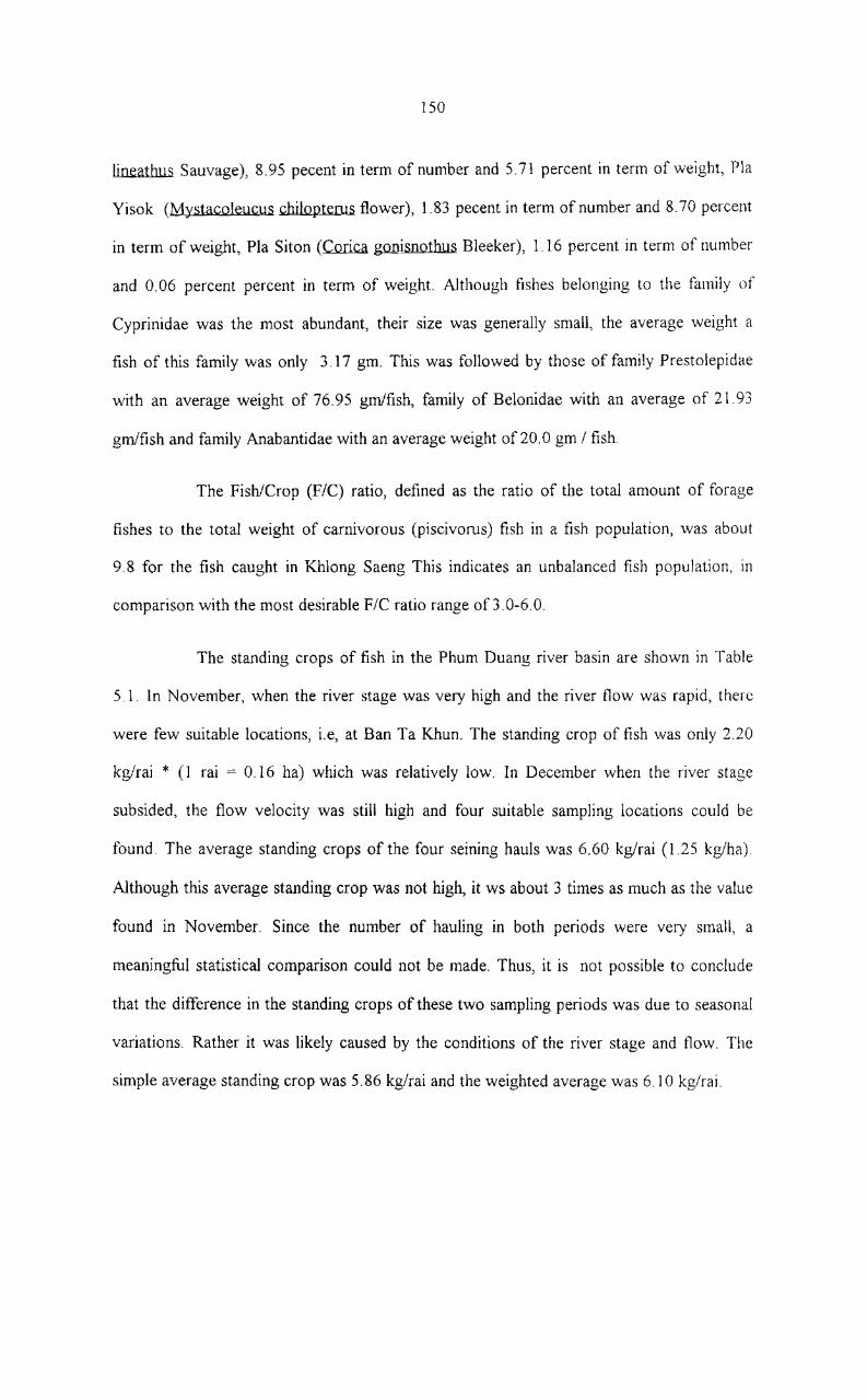
ISO

lineathus Sauvage), 8.95 pecent in term of number and 5.71 percent in term of weight, PIa

Yisok (Mystacoleucus cbilopterus flower), l. 83 pecent in term of number and 8.70 percent

in term of weight, PIa Siton (Carica gonisnothus Bleeker), 1.16 percent in term of number

and 0.06 percent percent in term of weight. Although fishes belonging to the family of

Cyprinidae was the most abundant, their size was generally small, the average weight a

fish of this family was only 3.17 gm. This was followed by those of family Prestolepidae

with an average weight of 76.95 gm/fish, family of Belonidae with an average of 21. 93

gm/fish and family Anabantidae with an average weight of20.0 gm I fish.

The Fish/Crop (F/C) ratio, defined as the ratio of the total amount of forage

fishes to the total weight of carnivorous (piscivorus) fish in a fish population, was about

9.8 for the fish caught in Khlong Saeng This indicates an unbalanced fish population, tn

comparison with the most desirable FIC ratio range of3.0-6.0.

The standing crops of fish in the Phum Duang river basin are shown in Table

5.1. In November, when the river stage was very high and the river flow was rapid, there

were few suitable locations, i.e, at Ban Ta Khun. The standing crop of fish was only 2.20

kglrai * (1 rai = 0.16 ha) which was relatively low. In December when the river stage

subsided, the flow velocity was still high and four suitable sampling locations could be

found. The average standing crops of the four seining hauls was 6.60 kg/rai (I.25 kg/ha).

Although this average standing crop was not high, it ws about 3 times as much as the value

found in November. Since the number of hauling in both periods were very small, a

meaningful statistical comparison could not be made. Thus, it is not possible to conclude

that the difference in the standing crops of these two sampling periods was due to seasonal

variations. Rather it was likely caused by the conditions of the river stage and flow. The

simple average standing crop was 5.86 kglrai and the weighted average was 6.10 kg/rai.

'\~

P~I"

' .. ~

~,.

'J,,\.( 0

••

-------_

.-

"g .~

N ~, ~

FIG

UR

E 5

.1

PL

AN

KT

ON

AN

D F

ISH

PO

PU

LA

TIO

N I

N P

HU

N D

UA

NG

BA

SIN

LEG

EN

j) .

o So

mpli

n~

loco

lIon

---<

:"<

Slr

.am

• A

mph

o.

Roo

d

Rai

lway

-l-O

o'n'5I

:~ , .

o 0

GRto

P~"'

IC

SCA

LE

v,

IS

"m

152

TABLE 5.1

ST ANDING CROPS OF FISH POPULATION IN PREVIOUS INVESTIGATION

(DECEMBER 1980)

Location Area Anclosed Total Fish Standing Crop,

m2 Caught, kg kg/nli

1 Ta Khun village 1,600 2.195 2.20

2 Bang Kaew village 1,920 18.006 15.01

"" Bang Kaew village 1,280 4.721 5.90 .J

4 Bang Kaew village 1,760 3.340 3.04

5 Bang Khian village 1,440 6.291 6.99

6 Hat Khan village 1,600 2.036 2.04

Average - - 5.86*

Notes (1) * Simple average

(2) Weighted average = 6.10 kg/rai

Source Environmental and Ecological Investigation Report.

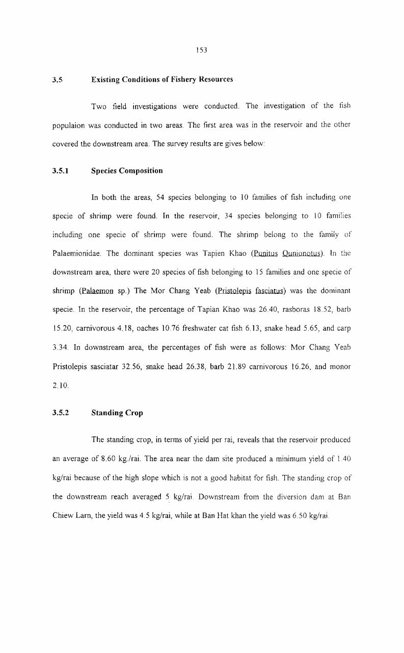
153

3.5 Existing Conditions of Fishery Resources

Two field investigations were conducted. The investigation of the fIsh

populaion was conducted in two areas. The first area was in the reservoir and the other

covered the downstream area. The survey results are gives below:

3.5.1 Species Composition

In both the areas, 54 species belonging to 10 families of fish including one

specie of shrimp were found. In the reservoir, 34 species belonging to 10 families

including one speCIe of shrimp were found. The shrimp belong to the family of

Palaemionidae. The dominant speCIes was Tapien Khao (Punitus Qunionotus). In the

downstream area, there were 20 species of fish belonging to 15 families and one specie of

shrimp (Palaemon sp.) The Mor Chang Yeab (Pristolepis fasciatus) was the dominant

specie. In the reservoir, the percentage of Tapian Khao was 26.40, rasboras 18.52, barb

15.20, carnivorous 4.18, oaches 10.76 freshwater cat fish 6.13, snake head 5.65, and carp

3.34. In downstream area, the percentages of fish were as follows: Mor Chang Yeab

Pristolepis sasciatar 32.56, snake head 26.38, barb 21.89 carnivorous 16.26, and monor

2.10.

3.5.2 Standing Crop

The standing crop, in terms of yield per rai, reveals that the reservoir produced

an average of 8.60 kg./rai. The area near the dam site produced a minimum yield of 1.40

kg/rai because of the high slope which is not a good habitat for fish. The standing crop of

the downstream reach averaged 5 kg/rai. Downstream from the diversion dam at Ban

Chiew Lam, the yield was 4.5 kg/rai, while at Ban Hat khan the yield was 6.50 kg/rai.

154

TABLE 5.2

STANDING CROP OF FISH IN RAJJAPRABHA RESERVOIR

AND DOWNSTREAM AREA

Area Location Total Caught, Area, rai Standing Crop

(gm) (1,600 m2) kg/rai

Reservoir Bang Kaew village 1024 1 10.24

Bang Khian village 696 1 6.96

Average 860 1 8.60

Downstream Ban Chiew Lam 350 1 3.50

Ban Hat Khan 650 1 6.50

Average 500 I 5.00

Note The information is derived from the fIshery survey results conducted in this

study.

3.5.3 Preliminary Comparison of Fish Population during the Pre and Post

Impoundment Periods

The number of fish species has decreased from 93 specIes before the

impoundment to 54 species after impoundment. However, this may either be due to the

change in the environment or the collecting technique. A change in environment 176 can

cause a change in fish species, i.e., riverine to Iucustine species. In the reservoir, the

dominant species found during the pre impoundment study was PIa Siew (Rasbora rasbora)

and the dominant specie found during the post-impoundment period was PIa Tapien Khao

(Puntius gonionotus).

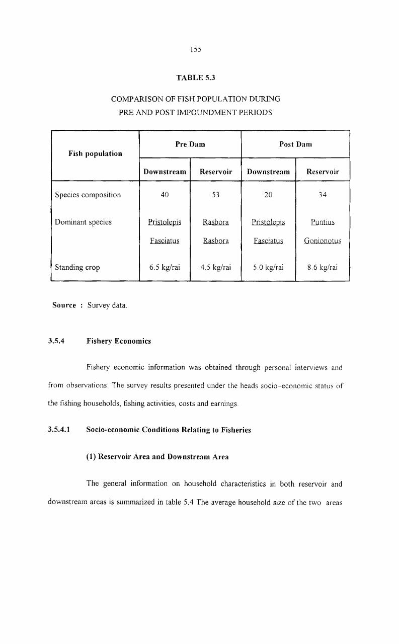
155

TABLE 5.3

COMPARISON OF FISH POPULATION DURING

PRE AND POST IMPOUNDMENT PERIODS

Pre Dam Post Dam Fish population

Downstream Resel-voir Downstream Reservoir

Species composition 40 53 20 34

Dominant species Pristolepis Rasbora Pristolepis Puntius

Fasciatus Rasbora Fasciatus Gonionotus

Standing crop 6.5 kg/rai 4.5 kg/rai 5.0 kg/rai 8.6 kg/rai

Source Survey data.

3.5.4 Fishery Economics

Fishery economic information was obtained through personal interviews and

from observations, The survey results presented under the heads socio-econotnic status of

the fishing households, fishing activities, costs and earnings.

3.5.4.1 Socio-economic Conditions Relating to Fisheries

(1) Reservoir Area and Downstream Area

The general information on household characteristics in both reservoir and

downstream areas is summarized in table 5.4 The average household size of the two areas

156

was 4.52 and 5,80 persons respectively. The proportions of males to females were almost

equal in both the areas, Fruit tree farming was the main occupation in the two areas. The

major supplementary occupations in the proposed reservoir area were driving of passenger

boats, and wage earning, Rice farming, merchandinsing and wage earning were the major

supplementary occupations in the downstream area. It is imporatant to note that no

household regarded fishery among the major supplementary occupations. In the reservoir

area, the average household income was 56,854 bahts/year and the average household

expense was 38,400 bahts/year. No data on this matter was given by the downstream

residents.

Table 5.5 presents the general information on fishing occupations among the

sample households in the reservoir and downstream areas. All of the households in the

reservoir area have participated in flsherey as their subsistence occupation, which only

61. 0 percent of the households in the downstream area caught fish for cash income. The

main fishing season for the reservoir residents is between January and May for the

downstream residents is between December and May. But the reservoir residents caught

fish primarily during the main fishing season, while the downstream residents operated

fishing activities all year round. The monthly average fishing trips were 8 and 15 for the

reservoir and downstream households respectively.

The average numbers of hours spent on each trip were 12 and 6 respectively,

and the average number of family members participating in fishery activities were 2 for

both the groups. Hence, the fishing effort of the downstream residents was more than twice

the effort of the reservoir residents, averaging 2,160 hours per year compared with 960

hours per year of the reservoir residents.

TAB]:;E5.4

GENERAL INFORMATION OF SAMPLE HOUSEHOLDS IN RESERVOIR

AND DOWNSTREAM AREA

Information Upstream Downstream

1. Total no. of households surveyed 70 60

Percent of total households 25.0 10.6

2. Average household size, persons 4.52 5.80

3. Average no. of children per household 2.42 3.00

4. Sex

Male (%) 49.69 46.85

Female (%) 50.31 53.15

5. Religion

Buddhism (%) J 00.00 100.00

Muslim (%) - -

6. Main occupation Fruit tree Farming Fruit tree Farming

7. Average no. of years participating in

Main occupation 13 >20

, 8 Major supplementary occupations Boat driving Mineral Rice fanning

Prospecting Merchandising

Wage earning Wage earning

9. A verage household income, baht/year 56,854 No data

10. Average household expense, baht/year 38,400 No data

Source: Surat Thani Provincial Fisheries Office.

158

TABLE 5.5

GENERAL INFORMATION ON FISHING OCCUPATION OF HOUSEHOLDS IN

UPSTREAM AND DOWNSTREAM AREA.

Information Reservoir Downstream

1. Average percentage of household participating

in fishing activities 100.00 100.00

2. Status of fishing occupation *

As main occupation (%) - -

As supplementary cash income (%) - 39.00

As subsistence occupation (%) 100.00 61.00

.., Main fishing season Jan-May Dec-May -'.

4. Major fishing ground Reservoir Phum Duang

5. Time spent on fishing River

Average no. of months per year 5 12

Average no. of trips per month 8 15

Average no. of hours per trip 12 6

6. Average no of family members used in fishing 2 2

Note As percentage of the total number of sample size in each location.

Source Surat Thani Provincial Fisheries Office

159

Twenty four different types of fishing gear were observed and described by

local residents. The most important ones included set gill net, cast net, and set line. The

percentages of the major types of fishing gear used in Phum Duang river are summarized

below:

Fishin2" Gear

Cast net

Set gill net

Set line

Bamboo trap

Boat trap

Others

Total %

Percent of Total

Reseryoir Area Downstream Area

40.0 80.0

30.0 10.0

20.0 0.0

5.0 0.0

0.0 1.0

5.0 9.0

100.0 100.0

The average catch per trip of households in the reservoir area was 28 kg, which

was 7 times as much as the average catch in the downstream area inspite of the fact that the

average time spent for each trip in the former area was only twice that of the latter area.

The average fish catche per month in these two areas were found to be 224 kg and 60 kg

respectively. The value of which was 2,600 baht and 675 baht respectively Barb

(Osteochilus spiropJeura) was the most important specie in both the areas, while catfish

(Mystus nemeus) was equally important catch in the downstream area. Other important

commercial fish species included barb (Puntius gonionotus), black shark barb (Morulius

chrysophekadion), featherback (Notopterus borneesis), and others (mainly forage fish).

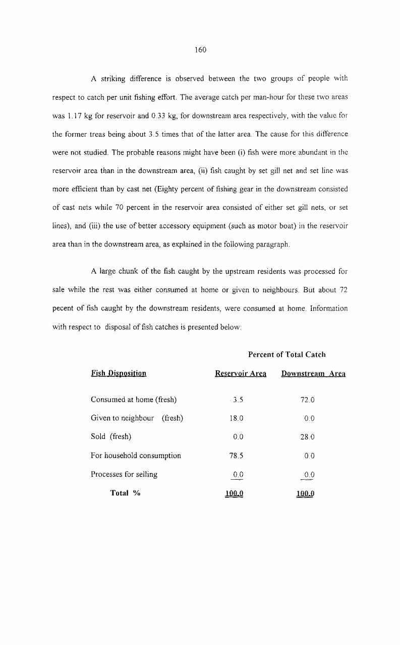
160

A striking difference is observed between the two groups of people with

respect to catch per unit fishing effort. The average catch per man-hour for these two areas

was 1.17 kg for reservoir and 0.33 kg, for downstream area respectively, with the value for

the former treas being about 3.5 times that of the latter area. The cause for this difference

were not studied. The probable reasons might have been (i) fish were more abundant in the

reservoir area than in the downstream area, (ii) fish caught by set gill net and set line was

more efficient than by cast net (Eighty percent of fishing gear in the downstream consisted

of cast nets while 70 percent in the reservoir area consisted of either set gill nets, or set

lines), and (iii) the use of better accessory equipment (such as motor boat) in the reservoir

area than in the downstream area, as explained in the following paragraph.

A large chunk of the fish caught by the upstream residents was processed for

sale while the rest was either consumed at home or given to neighbours. But about 72

pecent of fish caught by the downstream residents, were consumed at home. Information

with respect to disposal of fish catches is presented below:

Fish Disposition

Consumed at home (fresh)

Given to neighbour (fresh)

Sold (fresh)

For household consumption

Processes for selling

Total %

Percent of Total Catch

Reservoir Area Downstream Area

3.5 72.0

18.0 0.0

0.0 28.0

78.5 0.0

0.0 0.0

l.O..QJl lilll...D

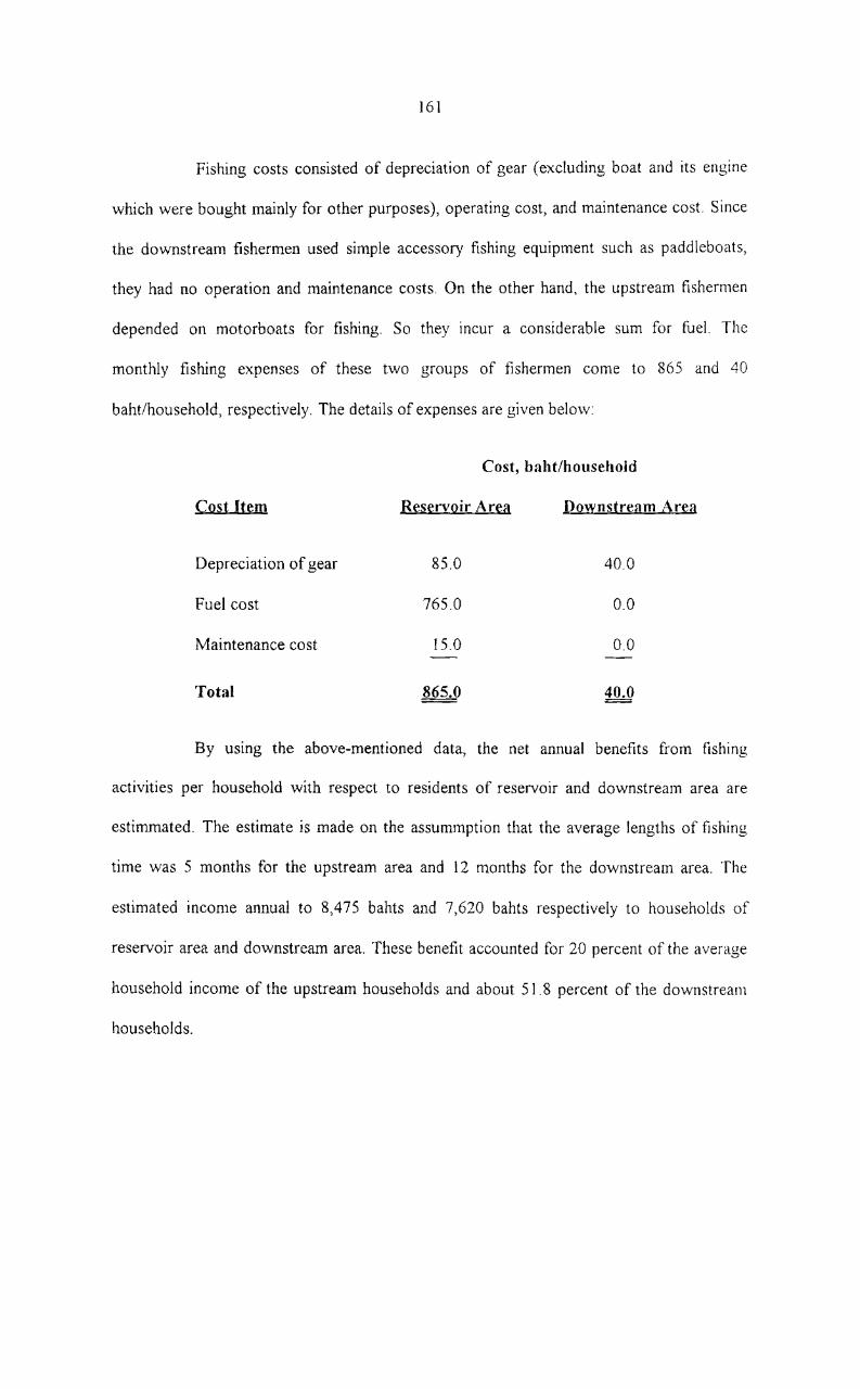
161

Fishing costs consisted of depreciation of gear (excluding boat and its engine

which were bought mainly for other purposes), operating cost, and maintenance cost. Since

the downstream fishermen used simple accessory fishing equipment such as paddleboats,

they had no operation and maintenance costs. On the other hand, the upstream fishermen

depended on motorboats for fishing. So they incur a considerable sum for fuel. The

monthly fishing expenses of these two groups of fishermen come to 865 and 40

baht/household, respectively. The details of expenses are given below:

Cost Item

Depreciation of gear

Fuel cost

Maintenance cost

Total

Cost, baht/household

Reservoir Area

85.0

765.0

15.0

865.0

Downstream Area

40.0

0.0

0.0

40.0

By usmg the above-mentioned data, the net annual benefits from fishing

activities per household with respect to residents of reservoir and downstream area are

estimmated. The estimate is made on the assummption that the average lengths of fishing

time was 5 months for the upstream area and 12 months for the downstream area. The

estimated income annual to 8,475 bahts and 7,620 bahts respectively to households of

reservoir area and downstream area. These benefit accounted for 20 percent of the average

household income of the upstream households and about 51.8 percent of the downstream

households.

162

(2) In Delta Area of Ao Ban Don

Fishing activities are carried on in a sail scale basis in the delta area of Ao Ban

Don at Pak Nam Phum Duang. Fishing activities here are greater than the subsistence

fisheries operated by the residents in the upper part of the Phum Duang river. Fishery

activities here are carried out year round with at least 20 fishing trips per month. The main

types of fishing gear used include setline, cast net, and gill net, which are used for catching

giant freshwater prawns (Macrobrachium rosenbergii)

The average fish catch came to about 60-100 kg of fish per boat per month.

The catch is mainly giant freshwater prawns. In this area, capital investment in fishing was

generally high commpared within the Phum Daung river. The monthly earnings from

fisheries here ranged from 8,000 and 14,000 baht per household.

(3) Some Additional Aspects of Freshwater Fisheries in Surat Thani

Aquaculture is not very popular in Surat Thani. In 1995, seventy-seven

households in this area carried out fish farming in a total area of only 10 rai, which

averaged about 208 m2 of fish farm per household (Department of Fisheries 1997). The

number of households carrying out fish farming increased to 127 in 1996 and the average

size of the farm per household stood at 213 m2. These average fish farm sizes were quite

small. Fish were raised exclusively in ponds, not in rice paddies, ditches, or cages.

The quantities and values of fish produced by aquaculture in these

two years are shown in Table 5.6. The table shows that the average fish yields were 1.03

ton/rai (134 kg! household) and 1.32 ton Irai (137 kg/household) respectively. And the

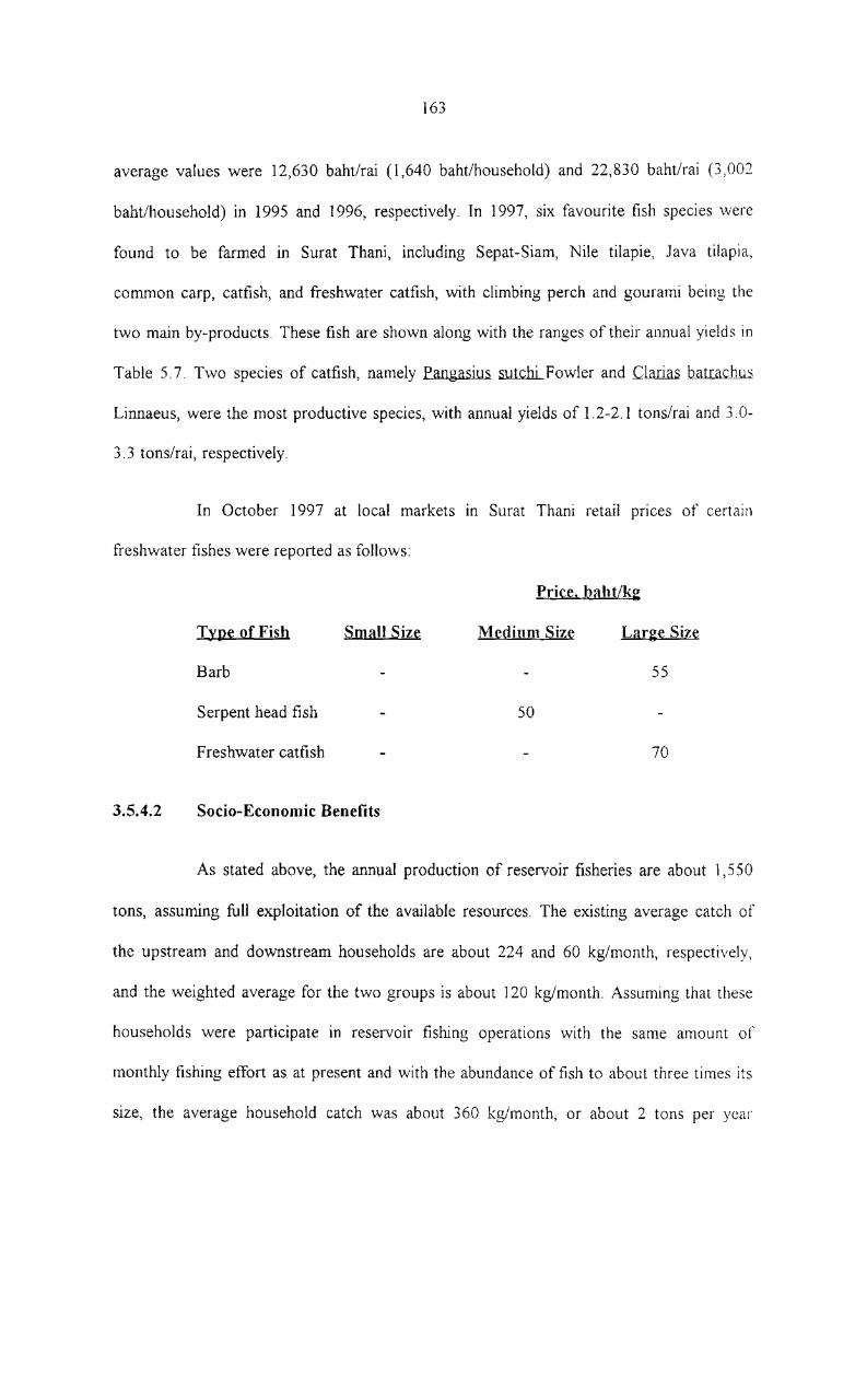
163

average values were 12,630 bahtlrai (1,640 baht/household) and 22,830 baht/rai (3,002

baht/household) in 1995 and 1996, respectively. In 1997, six favourite fish species were

found to be farmed in Surat Thani, including Sepat-Siam, Nile tilapie, Java tilapia,

common carp, catfish, and freshwater catfish, with climbing perch and gourami being the

two main by-products. These fish are shown along with the ranges of their annual yields in

Table 5.7. Two species of catfish, namely Pangasius sutchi Fowler and Clarias batrachus

Linnaeus, were the most productive species, with annual yields of 1.2-2.1 tons/rai and 3.0-

3.3 tons/rai, respectively.

In October 1997 at local markets m Surat Thani retail pnces of certain

freshwater fishes were reported as follows:

3.5.4.2

Type of Fish

Barb

Serpent head fish

Freshwater catfish

Small Size

Socio-Economic Benefits

Price, baht/k~

Medium Size

50

Lar~e Size

55

70

As stated above, the annual production of reservoir fisheries are about 1,550

tons, assuming full exploitation of the available resources. The existing average catch of

the upstream and downstream households are about 224 and 60 kg/month, respectively,

and the weighted average for the two groups is about 120 kg/month. Assuming that these

households were participate in reservoir fishing operations with the same amount of

monthly fishing effort as at present and with the abundance of fish to about three times its

size, the average household catch was about 360 kg/month, or about 2 tons per year

164

(assuming 6 months is spent on fishing and the other six months for crop cultivation).

Thus, about 750-800 households can participate in reservoir fisheries resulting in

considerable additional household incomes.

The fishing cost can be divided into two categories: operation costs and

depreciation costs. The operation costs consist of the expenses for fuel, lubrication, food,

fishing gear and maintenance costs. From the cost analysis it was found that the operation

cost was the major cost, being 85 percent of the total cost. It included about 50 percent for

the fishing gear cost and about 24 percent for the fuel cost. The average total cost of

fishing households was 113,960 bahts/year, while the average total sale was 140,000 bahts.

Hence each household had an average profit of 26,040 bahts/year with the rate of return of

18.6 percent.

The socio-economic benefits will be gained not only by fishermen, but \\·ill

also be shared by those involved in the fish marketing chain, including middlemen,

wholesalers, and retailers. While the benefits will exist along the line, it is also important to

provide measures which will prevent or minimize exploitation of fishermen by those

higher up in the market chain.

Due to steep slopes of the reservoir fringe area, it may be difficult for

fishermen to build permanent type of houses along the shoreline. Floating houses seem to

be more suitable in this particular case.

165

TABLE 5.6

PRODUCTION OF SOME FISH SPECIES CULTURED IN PONDS IN SURA T THAl'\JI

1995 1996

Fish Species Quantity, Value, Quantity, Value,

Ton Baht Ton Baht

Nile tilapia 4.5 68,800 12.9 small 236,300

Common carp 0.6 8,200 0 700

Thai carp 0 0 0 0

Sepat-Siam 0.2 2,400 5.5 300

Freshwater catfish 3.0 45,700 3.0 94,200

Serpent head fish 0 200 0.6 42,800

Tilapia 0.2 800 6,900

Total production 10.3 126,300 22.0 381,200

Average production, per rai 1.03 12,630 1.32 22,830

Ave. production, per household 0.134 1,640 0.137 3,002

Total No. of household 77 127

Total farm area, rai 10.0 17

Ave. farm size, m2/household 208 213

Source Fisheries Economic and Planning sub-division, Department of Fisheries.

166

TABLE 5.7

FAVOURITE SPECIES OF FISH RAISED IN PONDS IN SURAT THANI, 1997

Prod uctioll Common Name Scientific Name

(kg/rai/year)

Sepat-Siam Trichogaster pectoralis (Regan) 100 - 125

Nile tilapia Tilapia nilotica Linnaeus 150 -2 00

Java tilapia Tilapia mossambica Peters 120 - ) 75

Common carp Cyprinus carpio Linn 200 - 250

Catfish Pangasius sutchi Fowler 1,200 - 2, I 00

Freshwater catfish Clarias batrachus Linnaeus 3,000 - 3,300

Climbing perch* Anabas testudineus (bloch) -

Gourami* Trichogaster microlepis (Gunther) -

* By-product

Source Surat Thani Provincial Fisheries Office.

167

4. FORESTRY

4.1 Introduction

Forest vegetation plays an important role in an eco-system both from socio­

economic and ecological view points. In terms of socio-economics, forests provide timber

and other forest products which bring income to the rural people, as well as to the country

as a whole. Forest activities and forest industry partly help to alleviate labour force

problems. Moreover, forest land has long served agricultural growth, thus helping to

reduce pressure on land use for farmers. This results in an increase in occupation and

income and a reduction in social problems. Ecologically, forests are well recognized as the

best vegetative protective cover for watershed area, thus minimizing soil erosion and flood

problems. They also serve as moisture holding media and provide natural water storage

functions, which help regulate water flows throughout the year. Another very important

function of the forest is in serving as a habitat and food source for wildlife.

4.2 Objectives and Scope

Rajjaprabha dam was constructed during the years 1980-1987 and has been in

operation for about 10 years. It is at this early stage of operation this study on forestlY has

been carried out to assess environmental impacts which may have already been felt and to

suggest appropriate measures for minimizing further deforestation. The study covered the

following aspects.

Ca) Comparison of actual net benefits derived from forest clearing and the

value estimated before the project implementation.

168

(b) Plant community by speCieS, composition, relative abundance, and their

importance to fauna as habitat and food sources.

(c) Forestry management in the upper catchments area (agro-forestry and

wood plantation, etc.) before and after project implementation

(d) Rate of deforestation in the upper catchments area affecting soil erosion

and sedimentation in the watershed area.

(e) Actual budgets for forest protection In the upper catchments area and

forest clearing in the reservoir

The scope of the study covers the present status, the current trend, and the

potential of forest resources in the Phum Duang river basin. The study has been focused on

the upper catchment areas, including the resettlement area and reservoir, the power

transmission line right-of way, and other developments induced by the project.

4.3 Methodology

The method of investigation as following.

(1) General

(a) Review of information collected from various sources.

Cb) Interpretation of remote sensing data. False Colour Diazochrome images

with a scale of 1: 1,000,000 from LANDSAT were used to determine two

broad land use category, viz.; forestland and non-forest land. A random

ground check was also conducted.

( c) Economic evaluation of forest resources.

(d) Forecasting of future forest scenarios using available data.

169

(2) Field Investigation

For the vegetation community study, the upper catchment area of Phum Duang

river basin was categorized into 3 major land use types: (i) tropical rain forest, (ii) para­

rubber plantation and (iii) agroculture area.

A field investigation was conducted during 25-30 November 1997. For this

study, sample stands of 20 m x 20 m size were allocated at different elevations points, viz;

100, 200, 300, 400 m (msl), and in areas of different geological rock types (limestone,

shale and granite) in the tropical rain forest area. The following data was recorded in each

stand: (i) species composition, (ii) diamder at breast height (dbh) and height of each tree,

and (iii) species and number of individual seedling and saplings.

For the Para-rubber plantation, the same size of sample plots (20 x 20 m) were

identified in the same manner, but the selected elevations were 125, 200, 250, and 300 111

(msl). The diameters at breast height (dbh) and the heights of rubber trees within each plot

were measured. Species and number of individual plants under canopy or undergrowth

were also recorded. In agroculture areas, sample plots were marked at the elevations of

100, ISO, and 200 m (ms!).

In each sample stand (20 m x 20 m), the number and species of the upper trees

with diameter over 10 cm at breast height (1.30 m from ground level) were recorded. The

diameters were measured by using a diameter tape and the heights were measured by using

a comparative method with 5 m standard measuring tape. An 8m x 8 m sample plot was

randomly laid out in each sample stand and the number and species of saplings and shrubs

(dbh less than 10 cm ad height over 1.30 m) were recorded. For the under growth (tree

170

seedlings and other plant species with height less than 1.30), number and specIes were

recorded in a 2 m x 2 m sample plot within the sample stand. The elevation of the cent er of

each sample stand was measured by using an altimeter.

4.4 Review of the Previous Study

Prior to the implementation of the Rajjaprapha dam, environmental and

ecological investigations, including forestry study, were conducted in 1980. Emphasis was

on the catchment area of the damsite and the porposed reservoir area. Sample stands (20 III

x 20 m in size) were laid out to investigate comunities. The results are shown in Table 5 8

Moreover, a forestry inventory study was also conducted.

The results showed that the tropical evergreen forest, agrocultual area and

shifting cultivation and river bank area constituted, respectively, 66.10, 16.52 and 12.60

percent of the reservoir area at 110 m (msl) level. The rest was composed of cleared areas,

paddy fields, and agrocultural areas. The total volume of valuable timber was found to be

very small and considered to be of low value for logging. In total, the net value from

clearing both forest trees and all types of commercial trees in the reservoir area was found

to be 324.40 million bahts is shown inTable 5.9.

171

TABLE 5.8

FOREST TYPES IN THE RESERVOIR BEFORE IMPOUNDl'v1ENTATION

Land Use Type Area, ha 'Yc, of the total

l. Tropical Evergreen Forest 11,105 66.10

2. Riverbank forest 803 4.78

..., Shifting cultivation area .J.

Or secondary growth forest 2,117 12.60

4. Agro-cultural area 2,775 16.52

Total 16,800 100

Source Environmental and Ecological Investigation Report

172

TABLE 5.9

SUMMARY OF NET PROFIT FOR ALL TYPES OF TIMBER IN RESERVOIR

(Max, Elev. = 110 m MSL)

Type of Product Total Volume, Total Net Profit,

m3 baht

Sawtimber Grade A 449,632.2 177,900,000

Saw timber Grade B 414,741.0 84,600,000

Fuel wood 539,390,3 48,500,000

Bamboos 13,423,600.0* 13,400,000

Total - 324,400,000@

Notes (I) Estimated average price of fuel wood and bamboo

(a)

(b)

Fuel wood

Bamboo

(c) * in number of culms

90 baht/mJ

bahtl culm

Net Profit,

Baht/ha

10,600

5,000

2,900

800

19,300

(2) @ Total net benefit from logging timber from the entire area

Source Environmental and Ecological Investigation Report

173

4.5 Results of the Study

4.5.1 General Condition of Forest Resources

Forest type vegetation in the Phum Duang river basin covers an area of about

307,900 ha (3,079 km2), or 65.96 percent of the total area of the river basin. Table 5.10

illustrates forest classification in the watershed area, consisting mostly of terrestrial forest

(65.45 percent) and mangrove forest (0.51 percent). The terrestrial forests are classified

according to their physical and ecological characterstics as tropical rain forests.

The tropical rain forests were found distributed over the large area on the hills

on both banks of the river at elevations over 300 m (msl) and with slopes of more than 50

percent. The forest covers about 24 percent of the total areas is the upper catchment area.

About 42 percent of the downstream area the tropical rain forests were found distributed

over small hill tops with high slopes. The non-forest area forms about 158,900 ha, or 34

percent of the total area. The mangrove forest covers a total area of about 2,400 ha along

the shoreline, and in mud flat areas at the mouth of the canal and the Phum Duang river.

4.5.2. Forest in the Upper Catchments Area

The upper catchment area of the dam is located in Khlong Saeng subbasin.

General geography of this is hilly or mountainous with altitudes of more than 150 m (msl)

and slope of more than 40 percent. It covers about 143,500 ha, or about 30.8 percent of the

river basin. The population in the area number 12,638 or 5.1 percent of the total population

in the river basin, which consists of 50.89 males and 49.13 percent females The major

occupation of the people was in planting para-rubber and orchards.

174

TABLE 5.10

FORESTRY TYPES IN THE PHUM DUANG RIVER BASIN

Upper Lower Overall (~, of

Forest type Catchment, Catchment, River basin the total

ha ha ha

1. Forest area 1] 2,000 195,900 307,900 65.96

Tropical rain forest 112,000 193,500 305,500 65.45

Mangrove forest - 2,400 2,400 0.51

2. Non-forest area 31,500 127,400 158,900 34.04

Total 143,500 323,300 466,800 100

Source: Land use study in Chapter VI of this study.

4.5.3 Vegetation Communities

The upper catchmet area of Khlong Saeng sub-basin consists of an area of

143,500 ha (1,435 km2). The major land use pattern here is as follow: Tropical rain forest,

78 percent, agricultural land including para-rubber plantation and mixed orchards, 20

percent, abandoned land, 2 percent. The area covered by forest vegetation is normally

found on slopes greater than 50 percent and on hills tops of about 300 m (msl) in elevation.

The other areas have been encroached and occupied by local residents. Generally, they

divide the area into plots and cut down the trees in order to use the land for agriculture.

With regard to Para rubber plantations, new high yielding variety rubber trees are generally

planted. The remaining old variety rubber trees are found only in areas with high slopes

175

and in the national reserved forest area where the cultivators cannot get land title deeds. In

almost all deforested areas the inhabitants prefer to grow the new variety of rubber trees.

Mixed orchards are found in the areas with elevations not exceeding 250 m (msl),

especially in small lots of land located near living quarters and on stream banks.

Abandoned land is found scattered in sloping areas covered with grasses,

herbs, and small shrubs. Some areas were formerly used for agriculture and the regrowth of

some remaining vegetation can still be seen. Moreover, many areas are completely cleared

and are ready for cultivation.

In this study, the upper catchment area was divided according to elevation and

geological conditions. Sample plots were selected in representative areas of land use types.

These sample plots were randomly distributed throughout the area in the elevations ranging

from 100 to 400 m (msl) for field investigation. The results of vegetation community are as

follow.

(1) Tropical Rain Forest

Results of the study indicate that there are varIOUS speCIes of upper trees,

saplings, shrubs, and seedlings in the tropical rain forest. The density of stems was found

to vary from 400-500 trees/ha, averaging 458 trees/ha. Plant communities arc less abudant

at lower elevation than at higher elevations. The average density of plants is about 3,240

tree/ha. The common dominant plant species found in this type of forest were Shorca

leprosula, Shorea faguetjana, Saraca sp.. lntsia palembanica, Fissistigma bicolor,

Parashorea stellata, Aglaia andamanica, Gironiera sp.., Hopea s.p.., Hopea fr1:rul, Tetrameles

nudiflora, Dipterocarpus grandiflorus, Hydnocarpus illicifoIius, Anisoptera oblonga.

176

Premna tometosa, Xylia kerrii. The density of the undergrowth show a decreasing trend as

elevation increase. This is due to the fact that vegetation at lower elevations has a better

chance to receive a greater intensity of light.

With regrad to the relation between forest and wildlife, in general, the forest is

a habitat and a food source of wildlife. In this study it was also found that many kinds of

vegetation, especially fruits, were food for wildlife, most notably birds. These vegetations

were: Castanosis javanica, Baccaurea motleyana, Pithecellobium jiriga, Termialia. chebula,

Bouea oppositifoJia, Artocams Lanceifolius, and I\1cingifera sp., etc. These vegetations

were found scattered throughout the study area. However, other types off vegetation such

as mixed orchards, are also food sources for the wildlife.

(2) Para-rubber Plantation

Para-mbber plantations are quite popular among the inhabitants of the upper

catchment area. This can be confirmed by the existing situation whereby rubber plantations

are found from the plain area near the river bank upward along the slopes to the hilltops.

Most of the para rubber plantations are the new, high yeilding variety which are promoted

by the Department of Agricultural Extension. The old variety of mbber tree was cleared

away before growing the new variety.

Results of the study show that the density of rubber trees in different areas does

not differ greatly. It ranges between 300 and 525 trees/ha. With an average of 438 trees/ha.

The old mubber trees are planted in areas at above 400 m (ms!) elevation with slopes

exceeding 60 percent. The density was low due to greater spacing requuirement, it can be

said that the density of rubber trees is less as elevations increase over 250 m (msl). The

basal area of the trees ranges from 10 to 30 m2/ha with an average of 20 m2/ha The

estimated timber volume varies from 174 to 574 m3/ha, averaging 368 m3/ha. The common

undergrowth species covering the plantation floor were rubber seedling (Hever

brasiliensis), Cru1.o.n £P., Rhynchosora £P., Euatorjum odoratum, Imerate cylindrica,

Lygodium olystachyum, aederia romentos, and Caryota mitis

When compared with the results of the previous study, the results of the present

study show higher values for some rubber tree characteristics. This is probably due to the

replacement of the rubber tree variety which resulted in the plantation being even in agc

and size structures, the introduction of soil and water conservation measures, and the

improved in management as promoted by the provincial agricultural extension oflice

(3) Agro-culture Area

The results of the study on the structural characteristics of the agroculture

indicate that the upper coverage species of trees commonly found were CD..oos. nucifera,

Durion £P., Artocarus chameden, Parkia speciosa, Coffea sp., Rambutan(Nehelium

laaceum) and M.usa £P. The under-growth was composed of seedlings of those trees

mentioned above, including £iP.N £p., Eupatorium odoratum, Combretum trifolistum,

Melastoma £P., Imperata cylindrica, Saccharum arundinaceum, Lygodium tlexuozum and

In general the agro-cultural area is not very dense depending on the type of

mmajor crop grown. The ground cover is in the range of 75-85 percent of the total area

used for agroculturaJ purposes. The types of agroculture commonly found are of mixed

types around living quarters and in rhe area near the river bank. The major structural

178

characteristics are similar at those described in the previous study. However, it can be said

that at present the managemment practices of the farmmers consist of the minimum

ammount of care and maintenance. This will not necessarily result in adverse effects to

amount land area used. It should be note that, with a mixed types of crop grown, the

structure of plant community looks similar to the natural habitat, i.e., the tropical rain

forest, with a higher species diversity and greater stability of the communities. Also a high

production per area can be expected in the long run.

4.5.4 Estimation of Forest Reduction

As about 36 percent of the present forest coverage in the river basin is located in

the upper catchment area, the forest reduction rate reported by the Royal Forestry Departent

for Surat Thani can be taken approximately as the reduction rate in the upper catchment area.

During the years 1980-1987, the period of the Rajjaprabha dam was construction and its

beginning of operation, the reduction rate of forest area averaged of 2.12 percent of the area

recorded in 1980, or about 6,528 rais. The average percentage of reduction was higher than

the average value for Surat Thani province or for the southern region, and even for the whole

country. There was deforestation in the settlement area for allocate land to the people in the

resettlement areas of Ban Pattana. The total area cleared was estimated by Rajjaprabha dam

officials to be 2,100 ha (personal communication). Moreover, there were roads constructions

in the resettlement area. Construction of the relocated highway No. 401 to replace the old

inundated road, and the deforestation for an area of 40 km around the dam construction site

which was estimated to be 6,400 ha. In addition, many people took advantage during the

construction period for illegal logging. This can be confirmed by statistics of confiscated

timber volume and total number of arrest cases. This indicates a higher timber volume

179

cofiscation during the construction period of about 50 percent compared to the recorded

volume of confiscation during the pre-project implementation period (1980-1987). Then, it

declined rapidly after la years of operation. The ratio of illegal logging in the upper

catchment area to that of the watershed area in terms of tmbers confisated, decerased from,

67 percent before the dam construction to 34 percent during the construction period, to only

3 percent during the reservoir operation period.

After the dam was put into operation, the reduction rate of forest area showed a

decreasing trend with an average of 2.20 percent during 1988-1996, or about 2,800 ha per

year. This is 44 percent of the annual forest reduction during the project construction time.

The decrease in forest area reduction in the upper catchment area might be due to poor

accessibility in the remaining forest areas being located on high hills. Moreover, the

number of valuable trees in the remaining forest area in the upper hills is also low

compared to the forest in the lower areas.

In conclusion, the reduction of forest area in the upper catchment area during

the year 1980-1996 was at an average rate of 2.60 percent of the total forest area or about

3,200 ha per year. During the period of construction and beginning of operation the

reduction rate was considerably higher, 3.2 percent or about 4,600 ha per year. Then it

decreased to 2.20 percent per year or 2,800 ha in the operation period.

An attempt is made to forecast forest area reduction in future under four

different scenarios. These are presented as Case A, B, C and 0 as follows.

Case A : An average reduction rate of 2.12 % per year based on the data

obtained during 1987-1996. The assumptions underlying this estimate is that the socio-

180

economic situation both in the river basin and in the upper catchment area continues to

have a similar trend as in the past 10 years. Therefore, demands for logs and land for

agriculture will also have a similar trend.

Case B: An average reduction rate of 1.06 percent per year, or half of the

value in Case A. This is based on the assumption that it is difficult to gain access to the

remaining forest area. Moreover, more effective measures are introduced for forest

management, such as the establishment of a national park, reforestation programmes, forest

protection unit, etc.

Case C An average reduction rate of 3. 16 percent per year. This is based on

the assumption that the socio-economic situation in the river basin and the upper catchment

area receives stimulation from external factors. Therefore, the demands for logs and land

for agriculture and various infrastructure also receIve a strong stimulation and have a

consequential impact on reducing forest area.

Case 0: Similar to Case A for 10 years, then the rate changes to Case B.

Management measures are not yet implemented but are in the preparatory stage during

the first 5 years. When they are implemented (e.g., reforestation, forest protection, etc.)

the reduction rate decreases according to Case B.

To forecast the remaining forest area, the following equation is used:

Where =

Fo (1 + rt

forest area at year n,

forest area at base year,

R

N

181

reduction rate, percent, having negative value according to

the assumptions used for the 4 cases,

number of year

The calculation results are presented in Table 5-11. From the 57.9 percent

forest area in the upper catchment area in ] 997 only 35.8 to 49.1 percent will remain in the

area by the year 2005, depending on the forest reduction rate. The future reduction rate that

depends on watershed management objectives and other related developments. For

example, the occurence of Case B depends on the establishment of the national park \vhich

is curretly under way, also to be many other proposed developments.

To serve as a guideline for promiting or planning future developments in the

upper catchment area, benefits and consequences of each investigated scenario arc

summarized as follows.

Case A: The benefits to be obtained are from timber, para rubber

production, and others which need the forest land as a production factor. However, it will

result in an increasing the trend of suspended soil concentration carried by runotf into the

reservoir.

Case B: The major benefits from the forest will be in terms of forest

protection which will be more efficient than at the present. Moreover, this will bcnetlt the

reservoir in reducing and controlling the sediment discharge into the reservoir. However,

this case will require an increased budget to be used in protection and conservation of i he

forest.

182

Case C: The major benefits to be obtained are forest production and

agricultural production, including some other man-made environment such as roads, and

living quarters, etc. In this case, no increase in budget is required in the protection and

conservation of the forest. However, the sediments discharge into the reservoir is expected

to be higher than in Case A.

Case D: The benefits in the first phase will be forest products according to

the capability of existing forest productivity and agricultural products. In the second phase,

there should be an increase in reforestation along with the application of protection and

conservation measures. This will ensure good long term result in regards to the useful

service life of the dam and reservoir.

4.5.5 Effect of Reduction of Forest Area on Soil Erosion and Sedimentation in

the Reservoir

Quantitative estimate of soil erosion in a river basin is usually derived from the

Universal Soil Loss Equation (United State Department of Agricultural, 1978).

A

Where A

R

RKL S CP,

computed soil loss per unit area; obtained by multiplication

of the remaining factors.

rainfall factor; the number of erosion index units (El-units)

in the period of consideration. The erosion index is a measure

of the erosive force of specific rain.

K

L

s

C

p

183

soil erodibility factor; the eroslOn rate per unit of erosion

index for a specific soil, in a cultivated continuoLls fallow on

a 9 percent slope, 22.1 m (72.6 ft) long.

slope length factor; the ratio of soil loss from the tield slope

length to that from a 22.1(72.6 ft) length on the same soil

type and grade.

slope gradient factor; the ratio of soil loss from the field

gradient to that from a 9 percent slope, on the same length.

cropping-management factor; the ratio of soil loss from a

field with specific cropping and management to that from the

fallow condition on which the factor K is evaluated.

erosion control practice factor; the ratio of soil loss with

contouring, strip cropping or terracing to that with straight

row farming, up and down slope.

As can be interpreted from the soil loss equation, the change in forest area will

effect the soil loss through the C-factor. The degree to which the reduction of the forest

area affects the soil loss cannot be explicitly determined because of the varying nature of

the other affecting factors in the soil loss equation. Without adequate data on all relating

factors in the upper catchment area, further attempts to quantitatively determine the

specific relation between the remaining forest area and soil erosion rate of the catchment

area would only generate misleading results.

With such limitations, preliminary evaluation based on available related data is

made for providing management guideline as follows.

184

(1) An environmental impact study of Rajjaprabha dam showed that the total

suspended sediment transportation at Phum Duang river within the 2,690 km2

catchment

area was 497,200 tons per annum. The depth of soil loss was estimated from the sllspencied

load plus 20 percent bed load at 0.17 mm per year. The sediment transport into the

reservoir was calculated to be about 0.22 mm per annum, which is relatively high as

compared to other basins in Thailand.

(2) The annual depth of erosion and annual sediment load of Phum Duang river

basin were still lower than the values recorded in the natural forest. It was also lower than

the recorded values of other types of forests in the northern and southern region with the

exception of the dry dipterocarp forests which have poor soil conditions. This is true in

both the periods before and after the dam was put into operation. Also, from a reservoir

sedimentation study in Chapter IV, it is concluded that, even though the sediment inflow is

increased by 32.5 percent, there is not going to be any appreciable change in uesful storage

in a 100 year period. The reservoir can be utilized at its full benefit as planned.

The information described above indicates that, even though the forest area at the

upper catchment area has a decreasing trend, the soil erosion and sedimentation rate is still

considerably lower than that of other catchment areas. Moreover, the erosion will not

significantly affect the reservoir operation during the 100 years period. Therefore, it can be

concluded that the reduction of forest area in the upper catchment area at present has not

caused any significant impact regarding sedimentation in the reservoir. However, deforestation

should be terminated in order to avoid future adverse impact. Management measures,

therefore, should focus on protection and conservation particularly of the steep slope areas

(over 40 percent slope) which cover about 42 percent of the upper catchment area.

185

TABLE 5.11

FORECAST OF FUTURE FOREST AREA IN THE CATCHMENTS AREA

Case A Case B Case C Case 0

Area % Area 0/0 Area I}"O Area {}"o Year

Km2 UCA Km 2 UCA Km2 UCA Km 2 UCA

1120.00 57.17 1120.00 57.17 1120.00 57.17 1120.00 57.17 1997

1096.49 55.97 1108.25 56.57 1084.74 55.37 1096.49 55.97 1998

1072.98 54.77 1096.49 55.97 1049.47 53.57 1072.98 54.77 1999

1049.47 53.57 1084.74 55.37 1014.21 51.77 1049.47 53.57 2000

1025.96 52.37 1072.98 54.77 978.95 49.97 1025.96 52.37 2001

1002.46 51.17 1061.23 54.17 943.68 48.17 1005.20 51.31 2002

978.95 49.97 1049.47 53.57 908.42 46.37 984.43 50.25 2003

955.44 48.77 1037.72 52.97 873.16 44.57 963.67 49.19 2004

931. 93 47.57 1025.96 52.37 837.89 42.77 942.90 48.13 2005

Case A reduction rate - 2.12 %/year

Case B reduction rate - 1.06 %/year

Case C reduction rate - 3. 16 %/year

Case 0 reduction rate - 2.12 %/year for the first 5 years and -1.06 %/year

UCA Upper catchment area.

186

4.5.6 Forest Economics

The objective of forest economics evaluation is to estimate damage as well as

values generated from different causes to the forest in monetary terms Basic data,

especially sale price of log and productivity of the forest, are based on the results of the

pre-impoundment environmental study prepared in 1980. The reason for this is that the

damage values estimated for the year 1980 are also required for comparison purposes.

(1) Damages of Forest due to the Invasion of People

Damages of forest caused by the invasion of people can be estimated by using

the forest productivity data from the survey results of the Royal Forestry Department. It

was assumed that generally the forest condition in the upper catchment area is distributed

unrevenue and has very low tree abundance. This is due to the fact that large valuable trees

have already been cut down which in turn, has resulted in the invasion of people to use the

land for agricultural purposes. By using the average productivity of a forest of 0.12 mJ/ha

and other data obtained in this study, the following analyses are made.

(a) Period before and during construction: It was found that the reduction in

forest area averaged 6,528 ha per year or 783.4 m3 in terms of timber volume. The

monetary value for this can be estimated using an estimated sale price of 950 bahts/m3 as

follows:

value of forest damage 783.4 x 950

744,230 bahts/year.

(b) During operation period: It was found that the reduction in forest area was,

on an average of2,864 ha per/year or 343.7 m3 in terms of timber volume.

187

value of forest damage 343.7 x 950

326,515 bahts/year.

From the above analysis, it can be concluded that the value of forest damage in

the operation period is about 43.9 percent of the value in the pre-project implementation

period.

(2) Damage of Forest Caused by Illegal Logging

Timber volume confiscated from illegal logging activities and the price data at

689 bahts/m3 (Team Consulting Engineers, 1980) are used for evaluating the damage

value. It was found that before the operation period (1980-1987), the timber volume from

illegal logging was 145.6 m3/year, while in the post-impoundment period (1987-1996), the

average volume was 5.6 m3/year. The average of the two periods was estimated at 110.8

m3/year. From these data, the damage values can be calculated as follow:

Damage value of forest in the

pre-impoundment period 145.6 x 950

138,320 bahts/year.

Damage value of forest in the

post-impoundment period == 5.6 x 950

== 5,320 bahts/year.

Damage value of forest averaged

during 1980-1996 == 87 x 950

== 82,650 bahts/year.

188

The above data indicate a difference in damages to the forest caused by

illegal logging between the pre-and post-impoundment period. In general the efficiency of

illegal logging is considerably low. This is due to the fact that only good quality and

valuable trees are selected and cut down in order to get a high price. Moreover, careful

logging practice is always neglected, this results in damages to small trees and to natural

breeding condition of the forest.

With regard to the evaluation in (I) and (2) it can be concluded that in the prc­

impoundment period the damage value caused by the invasion of people and illegal

logging was about 0.64 million bahts/year. In the post-impoundment period the damage

value has dropped to about 0.24 million bahts/year, or 38 percent of the damage in the pre­

impoundment period.

(3) Damage to Vegetation Communities in the Inundated Area

The evaluation of forest economiCS III the inundated area is based on the

data from the 1980 study. Forest economics is re-evaluated due to the fact that the previous

study emphasized the analysis of economic feasibility on investment cost rather than forest

economics itself. During the construction period, it was found that there was also logging

in the settlement areas. The timber volume taken from the total areas of 2,727 ha was

estimated at 6,727 m3 Using the unit investment and the timber value data from the study

in 1980, the net benefit oflogging can be estimated as follows.

Investment cost 540 bahts/m3 x 6,727 m3

3,632,580 bahts

189

Benefit

The net benefit obtained

950 bahts/m3 x 6,727 m3

6,390,650

2,758,070

bahts

bahts.

When this net benefit is compared with the timber value of about 1.54

million bahts, the resulting damage value of forest due to the dam construction comes to

about 0.53 million bahts, or 34.7 percent of the total estimated damage value of the forest.

An interview with the official responsible for clearing the area around the dam

site during the construction period revealed that it took about 6 months in 1979 to clear an

area of 8.22 km2, or about 14.3 percent of the total reservoir area. The vegetation in the

clearing area was mostly para-rubber, the remainder were forest and other agricultural

products.

The para-rubber plantation in the inundated area included a productive area of

about 27.77 km2, with about 156,000 para-rubber trees (Team consultant Co. Ltd.

1980). The income arising from this in terms of rubber sheets, was estimated at 3.75

million bahts/year. During the construction period, the farmers could still receive benetit

from the rubber production until the impoundment began in 1987. Therefore, during the 7

year period of the dam construction it can be estimated that the farmer still benefited from

rubber production at 13.4 million bahts (1980 price). After that no benefit was obtained

due to the impoundment and project operation. The total damages were estimated at 36.3

million bahts less, or 22.9 million bahts or 63 percent of the total damages, as previously

estimated.

The para-rubber trees in the cleared area of 5 km diameter in the year 1987

covered an area of about 5.15 km2. It is estimated that about 28,930 rubber trees with a

190

timber volume of about 25,430 m3 were cleared and burnt. If these rubber trees were all

taken out of the inundated area and used for chip board production, for fuel in mining

industry, and for charcoal production, at an estimated local market price of 20 bahts/m1

,

the total value would be about 0.5 million bahts. Subtracting this value from the value

estimated in pre-impoundment (2.7 million bahts), the para ruber trees in the inundated

area would be valued at 2.2 million bahts.

In conclusion, the construction of the Rajjprabha dam is re-estimated to result

in 0.53 million bahts damage to the forest and 25. 1 million bahts damage to Para-rubber

plantation. The total damage would be 25.6 million bahts, significantly less than the

damage estimated prior to the dam construction.

(4) Damages Caused by Transmission Line

AilS kV transmission line from Rajjaprabha power plant to Surat Thani

substation is about 70 km and 20 km from powerhouse to main junction line. A strip 50 m

wide along the line has been cleared for safety purpose, which amounts to about 7.28 km2 or

728 ha. The results of a field survey revealed that most of the forest area, as previously

mentioned, had already been invaded and replaced by Para-rubber plantation during the pre­

construction period itself. The remaining forest area is on the hill tops oflimestone formation

with moderate to steep slopes unsuitable for cultivation. Therefore, it can be concluded that

the impacts from the transmission line to the forest are practically negligible.

(5) Benefit from Timber Cutting

Total benefit from timber logging in the overall reservoir area before

impoundmentation is estimated at about 324,400,000 bahts (19,300 baht/ha).

191

(6) Economics of Uncut Forest

The average increment of forest stock for the whole country, which was

studied by M.D Backer for the RFD is used as the basis. This study estimated the average

increment of a tropical ever green forest to be about 2.5 percent. By multiplying 0.025 (25

percent) with the growing stock volume of the forest in the reservoir area, the total annual

increment is estimated at 35,094 (2.09 m3/ha).

The future value of net income are calculated as shown in Table 5.12 along

with the expectation values of the uncut forests. Economically speaking the expectation

value, sometime called net present worth, of an investment is the net value at some point in

time (usually at present) of expected future incomes that have been discounted back to that

time at a give rate of interest. This value is utilized in estimating the present of future net

worth of an interest. For project evaluation, the expectation value of the future net worth of

different investment alternative can be compared to select the most desirable program.

In case of the Rajjaprabha project, the present values of agro-cultural and forest

products are estimated, based on the criteria given previously, to be about 89.51 million

bahts for a 10 year period, 106.93 million bahts for 20 year period and 72.53 million bahts

for 50 year period.

These are direct benefits in which direct benefits, such as those from non-forest

products and wildlife resources, are excluded. Additionally, other factors, including

Increases in timber values due to inflation and due to benefits from forest clearing and

those from the uncut forests under the without project condition cannot be compared

because some of the most important aspects, environmental changes due the permanent

loss of the forest inundated are not included in evaluating the economic effects.

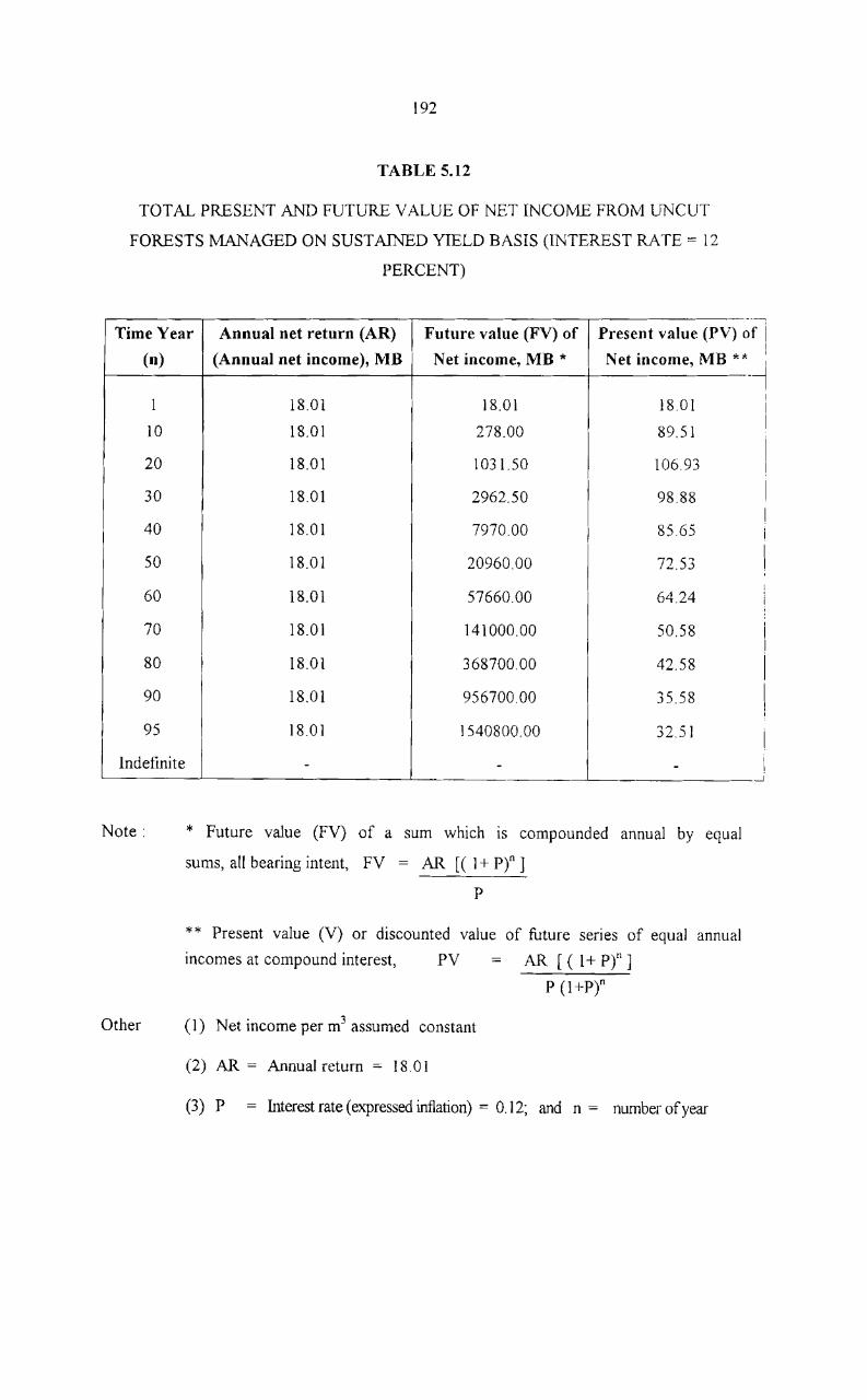
192

TABLE 5.12

TOTAL PRESENT AND FUTURE VALUE OF NET INCOME FROM UNCUT

FORESTS MANAGED ON SUSTAINED YIELD BASIS (INTEREST RATE = 12

PERCENT)

--Time Year Annual net return (AR) Future value (FV) of Present value (PV) 0

(n)

1

10

20

30

40

50

60

70

80

90

95

Indefinite

Note:

(Annual net income), MB Net income, MB * Net income, MB **

18.01 18.01 18.01

18.01 278.00 89.51

18.01 1031.50 106.93

18.01 2962.50 98.88

18.01 7970.00 85.65

18.01 20960.00 72.53

18.01 57660.00 64.24

18.0 I 141000.00 50.58

18.01 368700.00 42.58

18.01 956700.00 35.58

18.01 1540800.00 32_5 J

- - -

* Future value (FV) of a sum which is compounded annual by equal

sums, all bearing intent, FV = AR [( J + pr ] p

* * Present value (V) or discounted value of future series of equal annual

incomes at compound interest, PV AR [( l+Pt] P (1 +p)n

Other (1) Net income per m3 assumed constant

(2) AR = Annual return = 18_01

(3) P = Interest rate (expressed inflation) = 0.12; and n = number of year

-

f i I

~ i

I I

I

i -.J

193

5. WILDLIFE

5.1 Introduction

All development projects, along with generating benefits also creates certain

environmental and ecological problems. Generally, these ecological alterations may favour

some animals which carry problems for others at the same time. So only those wllo are

favoured and those who can adapted to the new condition can survive and multiply while

those less-adaptable become scarce and eventually become extinct from the area. So it is

important to know the ecological consequences of each development project, to initiate

remedial measures to minimise consequences.

5.2 Objective

The objective of the study regarding wildlife is to provide basic information

about the naturally existing wildlife after the constructed of the Rajjaprabha dam. This will

help to compare with the previously collected information in the pre-impoundment

environmental impact study and therefor help to ascertain changes in plant and animal

species in the area as results of the construction of the dam. The following aspects were

investigated during this study:

(a) Wildlife specIes composition and population of the wildlife in the

watershed and the reservoir areas including their status as resident or

migrant.

(b) Plant communities and species abundance in relation to fauna for habitat

and food sources.

( c) Suitable and unsuitable habitats for wildlife in the two zones.

194

5.3 Study Area and Method

5.3.1 Concern of the Study

This study concerns mainly 4 groups of vertebrate animals, i. e. birds, mammals,

amphibians and reptiles. Surveys and samplings for each group were conducted during two

field trips, representing the dry and wet seasons so as to obtain a better picture of year­

round wildlife existence. The first trip during the dry season from 25-30 March 1997,

while the second, was in wet season from 10-15 November 1997.

5.3.2 Study Method

An extensive survey was conduucted to ascertain the nature and evolution

of wildlife. The surveys were conduucted in day and night in the aquatic and terrestrial

habitats, in the rubber plantation and the original forests. In each site, 3 survey routes

(transections), each have 500 m long, were set for detailed using two main data-collecting

techniques.

(1) Direct Observation

Only easily recognized animals such as birds and mammals were observed

with the help of binoculars in the daytime and by torchlights in the nigh time along the 3

survey routes. The identity, abundance, preferred habitat and observed behaviour of the

wild animals were carefully recorded. This technique was supplemented by track finding,

animal remains inspection, and by interviewing the local inhabitants. Survey time of birds

were conducted from 6.00 a.m. to 9.00 a.m. and 3.00 p.m. to 6.00 p.m., which is

195

considered to be their periods of highest activity. In the case of nocturnal mammals,

amphibians and reptiles surveys were conducted during night.

(2) Collection

This technique reqUlres the actual procurement of the wild animals through

vanous methods. Because of the secretive habitats and similar appearances of some

animals groups, (for instance, bulbuls and the wild rodents), they should be studied from

close proximity to determine their exact identification. In some cases the captured animals

were sacrificed for internal autopsy for determining reproductive conditions. The following

three methods were used for collecting specimens.

(a) Netting: For birds and bats, six mist nets were used to collect specimens

in each survey route. Each net, 24 m long, was set up at an interval of 100 m, both day

and night, for collecting purpose.

(b) Trapping : Trappings were maded in the 3 survey routes, in catch 100

traps In each, for capturing small mammals during the night. Three successive night

catches from each habitat site were taken as a representation of the existing population

(c) Cruising Amphibians ad reptiles were obtained by the method of

intensive searching along the route. Every animal collected was studied in detail on all

pertinnet data concerning the capture, vegetable habitats, and the vertical and/or horizontal

position when first found.

196

5.4 Results of the Study

Wildlife study conducted in this post-environmental evaluation reveals Cl towl

of ],769 species, including 97 birds, 50 mammals, and 32 amphibians and reptiles. These

are presented in Table 5.12. The majority of birds are of residential status and only about

12 percent are of migrant type. The preferred habitat for the birds is rubber plantation.

Only 23 percent show high degree of forest dependence. The characteristic of

the rain forest in possessing a high resident species and low population density is evident.

About 52 percent of the bird species are regarded as rare and 24 percent very rare.

Of the 50 mammal speCieS reported in this study, about 80 percent were

observed and collected. The rest were identified from strategic interviews of reliable local

inhabitants. Here only the Asian Two-horned Rhinoceros is regarded as a preserved wild

animal. Twenty-two other mammals are classified as proteced wild animals, while some

are also treated as endangered by international agencies. The mammals in this area are

characterized by a high degree of forest dwellers (58 percent) and a high number of species

showing high forest dependence (50 percent).

Ten of the 32 species of the amphibians and reptiles are legally protected. Of

these protected species only the Malayan Giant Frog (Ranablythi) is regarded as the

protected wild animal under the game and food category. Of these only 10 species show

high degree of forest dependence.

Of the many fruit trees found growing in the area, those favoured by birds and

mammals are rose apple (Eugenia), Chinese lantern (Baccaurea), plum mango (~),

and mango (Mangifera). These favoured tree species are abundant in density (25-50

197

trees/ha.) The wild animals that seem to favour the artificial rubber plantation are Common

Wild Boar (Sus scrufu), Dusky Langur ( Presbytis obscura) and Malayan Flying Lemur

(Cynoceph alus variegatus). They feed on the fruits of the rubber trees or shelter in the

thick foliages of the rubber tree. In general, the food sources of wildlife are numerous in

species but less in individuals. A proposal to establish an area as a national park is

underway.

TABLE 5.13

WILD ANIMAL IN THE RIVER BASIN PRE AND POST 11v1POUNDMENTATION

Pre Post

impoundmentation impoundmentation Animal group

Species Species Genus Family

Birds 69 78 53 31

Mammals 38 50 39 23

Amphibians and reptiles 15 21 17 10

Total 122 149 109 64

Source Survey data

5.5 Wildlife Impact

The wildlife impact is non-quantifiable for two mam reasons. First it is not

possible to estimate the amount or number of animals affected by Raijaprabha dam. Second,

the value of wildlife are intangible. Without observation on people's willingness to pay for

enjoyment of wildlife, it is impossible to estimate economic value of the affected wildlife.

CHAPTER VI

HUMAN USE VALUE

CHAPTER VI

HUMAN USE VALUES

1. INTRODUCTION

Human use values are among the environmental values, which will be affected

by any large-scale development project, especially dams and reservoir projects.

Construction of dams is proposed to improve the water resource conditions in the project

area, which changes the existing conditions in the human utilisation of water. The

development of the reservoir project will affect the present land use pattern in the proposed

reservoir area and the planned project area. Provision of more stable water supply will

change the existing water use conditions in many ways, e.g. irrigation, water supply and

navigation. As related to the project development, a road system may also be developed

which may initiate changes in the existing transportation system. In the case of a

hydroelectric project, the power generation output will affect the electrical power supply

conditions of the region. Thus the impacts of the project on the human use values will be

one of prime importance to be evaluated in connection with project development.

For the Rajjaprabha project, the human use aspects taken into consideration

include (i) land use (ii) irrigation and water supply (iii) flood protection (iv) transportation

and navigation (v) power production and (vi) water pollution. These aspects are reviewed,

analysed and evaluated, item by item and presented in a sequential from the following

sections.

199

2. LAND USE

2.1 Introduction

In the environmental system of the river basin, land resources arc one of the

main resources for supporting lives, production, and human activities. The utilisation of

land is reflected by land use patterns which are the consequence of various environmental

conditions, i.e., soil fertility, water availability, topography, socio-economic condition, ete

In turn the use of land and its changes can affect other environmental elements, such as the

hydrologic regime, climate, human use values, and quality of life.

Land uses information and the consequences of land use changes are extremely

necessary for environmental evaluation. To obtain a complete picture of land use and

consequence in its long term change, the past information relating to the present land LlSC

pattern needs to be re-evaluated together with other related aspects which indicate land Llse

potential.

2.2 Objectives

The objectives of the land use study are:

(a) To identify the changes in land use in the resettlement and in the irrigation

areas after the implementation of the dam.

(b) To identify beneficial impacts of Rajjaprabha project to the application of

land use.

(c) To support information to other related studies.

200

2.3 Methodology

The study was conducted using the following methodology:

(a) Survey has been carried out using the 1: 5,000 scale aerial photos taken in

1995 and 1996 together with 1 :50,000 scale topographic maps. Aerial

photos were interpreted through mirror stereoscope employing deduction

methodology.

Cb) Reviewing the existing information on land use prior to the project

implementation.

(c) Improving the pre-impoundment land use information in the area.

(d) Evaluation of the land uses according to the objectives.

2.4 Land Use before the Project Implementation

2.4.1 Land Use in the Reservoir and Resettlement Areas

Land use in the reservoir and in the resettlement areas are classified into six

classes according to their purpose of use during the survey period, (Team Consulting

Engineers Co. L TD, 1980) Descriptions of these land use types are given below.

The reservoir covers an area of 172.44 km2 (17,244 ha). The major land use

types were: (1) forest area (69.32 percent), (2) farm land (12.84 percent), (3) old clearing

area (12.15 percent), (4) mixed orchard/residential area (2.82 percent), (5) rubber trees

(0.27 percent) and (6) water body i.e. canal (2.59 percent). The summary of area covered

by each type ofland use is presented in Table 6.1.

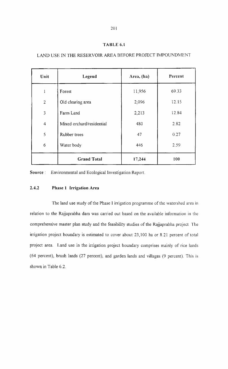
201

TABLE 6.1

LAND USE IN THE RESERVOIR AREA BEFORE PROJECT IMPOUNDMENT

Unit Legend Area, (ha) Percent

1 Forest 11,956 69.33

2 Old clearing area 2,096 12.15

3 Farm Land 2,213 12.84

4 Mixed orchardlresidential 480 2.82

5 Rubber trees 47 0.27

6 Water body 446 2.59

Grand Total 17,244 100

Source: Environmental and Ecological Investigation Report.

2.4.2 Phase 1 Irrigation Area

The land use study of the Phase I irrigation programme of the watershed area in

relation to the Rajjaprabha dam was carried out based on the available information in the

comprehensive master plan study and the feasibility studies of the Rajjaprabha project. The

irrigation project boundary is estimated to cover about 23,100 ha or 8.21 percent of total

project area. Land use in the irrigation project boundary comprises mainly of rice lands

(64 percent), brush lands (27 percent), and garden lands and villages (9 percent). This is

shown in Table 6.2.

202

TABLE 6.2

LAND USE IN IRRIGATION AREA, AS OF 1980

Legend Area, (ha) (Yt, of Total

Rice Land 14,700 64

Rice fields 10,100 44

Rice and sugar palm 450 2

Rice and anthills 2,050 9

Rice and shrubs 2,100 9

Brush Land 6,350 27

Shrubs 4,550 19

Mangrove like forest 1,500 7

Grass 200 1

Swamps 100 -

Garden Lands and Villages 2,050 9

House with garden 1,100 5

Village and garden 950 4

Total 23,100 100

Source Royal Irrigation Department (RID).

203

2.5 Present Land Use Pattern

The present land use pattern in the watershed area is found out from the

1: 15,000 scale aerial photos taken in 1996 and 1: 50000 scale topographic maps.

The watershed area which covers about 466,800 ha, includes the upstream and

downstream area of 143,500 and 323,300 ha respectively. Major land use in the watershed

area can be classified as forest (including tropical rain forest and mangrove forest), Para­

rubber plantation, mixed orchards (mainly coconut, mangosteen, rambutan, durian,

banana), paddy field, town and village, mines and non-productive or abandoned land.

Table 6.3 shows the present characteristics of land use types. These are described in the

following paragraphs:

(1) Forest : The forest area covers about 307,900 ha, which constitute

approximately 65.90 percent of the total basin area. The forest can be classified according

to its ecological condition. The forest in the upper watershed is terrestrial forest, which

covers about 112,000 ha. It is in the mountainous area, and is not suitable for agriculture.

The forest in the downstream area covers about 195,900 ha, which constitute mainly of

tropical rain forest on steep land on mountainous areas, and mangrove forest in the

estuarine area in the eastern part of the river basin.

(2) Para-rubber Plantation Para-rubber is the major crop lf1 the upper

watershed area. It is usually the first choice of the farmers for plantation. Thus those move

into the upland area by clearing the forest. Some of them are grown on steep land. The

Para-rubber plantation area covers about 59,600 ha, which forms approximately 12.77

percent of the total project area. This area consists of about 4,800 ha in the upper

watershed area, and about 54,800 ha, in the downstream area.

204

(3) Paddy Field : Because of the suitability of soils, topography, and water

condition rice can be grown only in the downstream area. From the survey it is found that

the paddy field area is constitute about 15,475 ha, which forms approximately 3 32 percent

of the total project area.

(4) Mixed Orchards : Mixed orchards cover about 3,880 ha in the upper

watershed area, and 34,200 ha, in the downstream area (8.16 percent of the total basin

area). They are generally native crops, and are concentrated around households. Many of

them are grown in the areas, which are not suitable for rice.

(5) Mine: Mine area is estimated at about 0.03 percent of the project area, or

about 165 ha, in the downstream area.

(6) Water Source Water source m the watershed area, (including the

reservoir, pond, river, and swamp) cover about 32, I 00 ha, which forms approximately 6.87

percent of the total area. This area consists of about 19,500 ha in the upper area, and about

12,600 ha in the downstream area.

(7) Non-productive and Abandoned Land: The present abandoned area is

about 890 ha in the upper watershed area and about 1,860 ha in the downstream area.

These form approximately 0.59 percent of the river basin area. The areas were abandoned

because of shifting cultivation and unsuitable physical or chemical soil condition.

(8) Town and Village: The river basin includes the area of Head Quarter,

Phra Nom district, Ban Ta Khun district, Khirirattha Nikhom district, Phun Phin district

and Muang Surat Thani district. Towns and villages cover an area of about 10,730 ha, i.e.,

approximately 2.30 percent of the total area. Of these about 2,430 ha are in the upper area

and about 8,300 ha, in the downstream area. They are composed of residential areas,

commercial areas, religious places, and industrial areas,

205

TABLE 6.3

PRESENT LAND USE IN THE PHUM DUANG RIVER BASIN

Land use type Upstream Downstream Overall river Percent of

area, ha Area, ha basin, ha the total

Water source 19,500 12,600 32,100 6.80

Forest 112,000 195,900 307,900 65.90

Rubber plantation 4,800 54,800 59,600 12.77

Mixed orchard 3,880 34,200 38,080 8.16

Paddy field - 15,475 15,475 3.32

Mine - 165 165 0.03

Non-productive and

abandoned land 890 1,860 2,750 0.59

T own and village 2,430 8,300 10,730 2.30

Total 143,500 323,300 466,800 100

Source Aerial Photos interpreted.

2.6 Change in Land Use Pattern

A comparison between the present land use and the land use prior to the project

implementation is made in order to identify the changes in land use after the

implementation of the dam, and to identify the beneficial impacts of Rajj aprabha proj ect on

the utilisation of the land. Since land use information prior to the project implementation is

available only for the reservoir and resettlement area and the Phase I irrigation area, direct

206

comparison is possible only in these areas. The changes in land use in the areas outside the

irrigation areas are not direct the impact of the project. It is rather the impact of other

factors that fall within the value of socio-economics factors, such as increase in population,

and political factors.

2.6.1 Change in Land Use in the Resen'oir and Resettlement Area

The pre-implementation information on land use in the reservOir and

resettlement area is very limited. On the basis of the available information the following

changes are noted.

Main portion of the area has been changed into water body. So also in the draw

down zone of the reservoir area. The remaining upland portion with rather steep slope has

partly been turned into resettlement areas. Since the topography, soil condition, and

climate are well suitable for upland crops, these areas have been altered from forestland

into rubber plantation and mixed orchards.

In the mountainous area there is not much change and to the area is still

covered by tropical rain forest. The changes In land use pattern 111 the reservOIr and

resettlement areas are shown in Table 6.4.

2.6.2 Change in Land Use in the Phase I Irrigation Area

Comparison of land use in the Phase I irrigation area before and after the

implementation of the project is summarised in Table 6.5.

207

TABLE 6.4

COMPARISON OF LAND USE IN THE UPSTREAM AREA BEFORE AND AFTER

THE DAM IMPLEMENTATION

Before After Area

Land use type Change

Area, ha % Area, ha tY;.

Paddy field 384 1.68 - - - 384

Mixed orchards 138 0.60 621 2.70 + 483

Rubber plantation 91 0.40 768 3.35 -+- 677

Old clearing area 336 1.46 143 0.62 - 193

Forest 21,896 95.25 17,920 78.05 -3,949

Water body 87 0.37 3,120 . J3.57 + 3,033

Village 56 0.24 389 1.69 + 333

Source The Environmental and Ecological Investigation Report and surveyed data.

208

TABLE 6.5

CHANGE OF LAND USE IN THE PHASE I IRRIGATION AREA BEFORE AND

AFTER THE DAM IMPLEMENTATION

Before After

Land use type Area

change Area, ha (% Area, ha (Y.,

Paddy field 14,700 63.60 15,475 67.0 +775

Mangrove like forest 1,500 6.50 1,340 5 80 -160

Shrub 4,550 19.70 3,500 15.15 -1050

Grass 200 0.87 125 0.54 -75

Swamp 100 0.44 60 0.26 -40

House with garden 1,100 4.77 1,350 5.84 +250

Villages and garden 950 4.12 1,250 5.41 +300

Total 23,100 100 23,100 100 ~

Source The Environmental and Ecological Investigation Report and survey data.

Presently, paddy field covers about 67 percent of the irrigated area (or

approximately 15,475 ha). This indicates an increase of only about 3.4 percent from the

previous condition. The nominal increase in paddy area is high due to the fact that area

suitable for paddy has already been used to the maximum extent.

209

House with garden, and villages and garden area has increased from 950 ha to

1,250 ha and from 1,100 ha to 1,350 ha, respectively, This accounts 5.14 and 5.84 percent

increase respectively. Corresponding the areas under shrub, grass, swamp and mangrove

forest decreased.

2.7 Economic Analysis of Para-rubber Plantation

In order to evaluate the benefits of land resources in the reservOir and

resettlement areas a basis economic analysis of Para-rubber are presented in Table 6.6

Table 6.6 presents the economic analysis of Para-rubber plantation per hectare.

The present value (at the first year of plantation) of net return is calculate at 87,700

bahts/ha while the annual equivalent net return in the 50 years period is 9,296.25 bahts/ha.

Table 6.7 Shows the economIC analysis of the agricultural potential in the

agricultural area for the assumed crop potential area of 8,768 ha. The total net return from

the agricultural potential discounted to the present amounts to 274.43 million bahts or the

annual equivalent of27.61 million bahts.

From the feasibility study of the project (ELC-Electroconsult, 1979) the net

benefit from irrigation development have been estimated about 200.4 million bahts on an

annual equivalent basis.

210

TABLE 6.6

ECONOMIC ANALYSIS OF PARA-RUBBER PLANTATION

(Interest rate = I 0 percent)

Yield Income Farm Net Year Note

(B / ha) (B/ha) Expenses (B/ha) Return

1 - - 11,393.75 -1823 Present value net

2 - - 6,112.5 -978 return

" 6,028.1 -964.5 -' - -4 - - 46,81.25 -749

= 87700Bha

5 - - 4,584.3 -733.5

6 800 14,400 3,053. ] 11,346.9 Annual

7 1,030 18,580 2,784.3 15,486.9 Equivalent

8 1,260 22,680 2,796.8 19,895.7 = 9,296.25 B/ha

9 1,420 25,560 3,053.1 22,763.2

10 1,520 27,360 3,053. I 24,310.9.

11 1,560 28,080 3,053.1 25,026.9

12 1,580 28,440 3,053.1 25,386.9

13 1,560 28,080 3,053.1 25,022.9

14 1,530 27,540 3,053.1 24,486.9

15 1,350 24,300 3,053.1 21,246.9

16 1,310 23,580 3,053.1 20,526.9

17 1,270 22,860 3,053.1 19,806.9

18 1,230 22,400 3,053.1 19,806.9

19 1,190 21,420 3,053.1 18,366.9

20 1,190 21,420 3,053.1 18,366.9

1 1 1 1 1 50 1,190 21,420 3,053.1 18,366.9

Source Rubber Replanting Aid Fund Board, Bangkok.

Year

1 2

~ir'

9

10

11

12

13

14

15

,11'

49

50

2) 1

TABLE 6.7

ECONOMIC ANALYSIS OF AGRICULTURAL POTENTIAL

(Interest rate = 10 percent)

Cash c.·op and Fruit Trees

Net

Return

(B/ha)

3,687.5 3,687.5

" 3,687.5

3,687.5

Area

(ha)

2,747 2,747

111'

2,747

2,476

2,476

"

2,476

2,476

Net

Retum

(M ») 10.13 10.13

1,

10.13

9.13

9.13

9.13

9.13

Panl-rubbe.·

Net Area

Return

(B/ha) (ha)

9,296.25 2,138 9,296.25 2,376

2,614

2,851

3,089

3,326

3,564

8,768

8,768

,,. " 9,296.25 8,768

9,296.25 8,768

Net

Return

(M B)

19.89 22.09

24.3

26.51

28.72

30.92

33.13

81.5

81.5

, 81.5

81.5

Total

net

Return

(M Ji)

30.02 32.22

34.43

36.64

38.85

41.05

43.26

91.63

91.63

" 90.63

90.63

Notes: (1) Assume a period of 50 year, which is the same as the economic life of the dam.

(2) From socio-economic survey off present net income per hectare.

(3) 2,747 ha are the present land available for agricultural development and

2,476 ha are assumed remaining land use for cash crop and fruit trees

212

2.8 Conclusion

Land use in the Phum Duang river basin is presently classified under seven

major types: (1) forest, (2) rubber plantation, (3) mixed orchards, (4) paddy field, (5) non­

productive and abandoned land, (6) mine area, and (7) town and village. The use of land

and changes in land use are largely due to a combination of various factors such as land

capability, water availability, prevailing agricultural technology, economic factors (ie,

market demand and pnces of agricultural produce) social and political reasons. The

implementation of Rajjaprabha project has induced thp, changes in land use mainly in the

reservoir area only. This was directly due to the impoundment of water in the reservoir and

the establishment of resettlement villages. The changes of land use in the downstream

areas are due to the introduction of irrigation and drainage systems, which increase

agricultural production potential in the areas. The choice of crops to be grown is, however,

determined mainly by the capability of land and economic conditions. The net benefits

resulting from land use development has been estimated to be 660 million bahts at 011

interest rate of 10 percent and for the 50 year period. This net benefit is 65 million bahts on

an annual equivalent basis.

213

3. IRRIGA TION AND WA TER SUPPLY

3.1 Introduction

The irrigation development of the Phum Duang river basin was part of a

comprehensive study carried out by the Royal Irrigation Department (RID). The phase 1

irrigation project to be developed along with the reserve consists ofI' an area of 23, 1 00 ha

located on the left bank of Khlong Phum Duang and Khlong Phun Phin. The irrigation

project is planned to be divided into 6 districts each to be served by a pumping plant

3.2 Irrigation

3.2.1 Objectives

aspects:

Objective of this study 1S to estimate irrigation benefit under four different

(1) Actual irrigation benefit realized at present;

(2) Potential or planned irrigation benefit;

(3) Beneficial estimates of water discharge to irrigation area achieved by the

project operation; and

(4) Irrigation benefit estimation by farm enterprise analysis.

All study aspects except the farm enterprise analysis are presented in this

section. The farm enterprise analysis, requires field data from socio-economic investigation

was described in the section on socio-economic.

214

An attempt is made here to assess and update relevant information on irrigation

component, emphasizing the progress in implementation and present and future trend of

irrigation water requirement.

3.2.2 Previous Investigation and Planning

Irrigation and agricultural development planning were done, and presented in

the June 1980 Environmental and Ecological Investigation (EEl) Report. The findings and

the formulated plans were later summarized in the EIS report. Relevant features planned

and presented were as follows paragraph:

The planned irrigation development scheme has been divided into two phases.

Phase I development plan called for the construction of the Rajjaprabha reservoir on

Khlong Saeng and diversion of parts of regulated water to irrigate .about 23,100 ha, with

double cropping by low lift pumping. Phase I irrigation area was on the left bank of

Khlong Phum Duang and Khlong Phun Ph in below the confluence of Khlong Van and

Khlong Phum Duang and extended down to the delta area. The Phase Il development,

suggested to be implemented 20 years after Phase 1, consisted of the creation of the Chiew

Krung reservoir on Khlong Yan, a diversion dam at Wat Nam Hak and 80 km irrigation

main canal to supply water for double cropping of 50,000 ha of which 13,280 ha, was

included in Phase 1.

Irrigation waters requirement averaged 98.4 mcm per year varying from 26

mcm in December to 24.2 mcm in March. Irrigation benefit estimated at 200.4.0 million

bahts per year (1980 value).

215

3.2.3 Results of the Study

(1) Updated Information on Irrigation Component

Rajjaprabha Irrigation Project presently being implemented by the Royal

Irrigation Department consists of the remaining components of the first stage of the overall

Phum Duang basin development, following the Rajjaprabha dam and hydropower

development in the headwater area. It has been planned mainly for irrigated agriculture

development of about 23,100 ha area in Surat Thani province. In addition, the project has

been planned for flood protection of the planned irrigation area and urban communities

along the Phum Duang river, for prevention of seawater encroachment into the loy"

agricultural land along the coast, and for fishery development. Another planned irrigation

area in the vicinity of the town of Surat Thani was also been planned for development as

the second phase, and that includes another diversion dam and 'distribution system for

irrigation on both banks of Khlong Phum Duang (Figure 6.1). This second phase has not

yet been implemented. The first phase of the Rajjaprabha Irrigation Project presently being

implemented consists mainly of:

(i) tidal canals

(ii) irrigation systems;

(iii) drainage systems;

(iv) flood control dike;

(v) service roads

(vi) on-farm works;

216

--~·20'--------------------------i------------------------.~------~------,L-------~~~~--~~~---4---1

LEGENO

~oJtcT IaOI.INO"'"

DtST"'I;'T lOUHO."Y

0 I"" I~ATION bl,TIltIC"t Ji"' .... t.

~ .S"t4I\LTIC ",AD

I ~ tiDAl.. C&MAL

'lOCD .IIIID TI DE. ""Onc1UH. UVI (

-- 9· 15' "41" 'ft'UGATIO .. CAHA\.

• ,"V"',.lNO IoT4TION

iif:Nl" ... L TI':!.HD Q# UUUCA.TtOlI4

C) U, .. ,,\I ITY $T~C" ."(A I 0 ~lLl"G( ----., - ---- 1IIIV[II:. STftU,W

0

'1g. hi'

I

FIGURE 6.1

IRRIGATION AREA

217

(2) Current Implementation I)lan and Progress

From the beginning of project construction in the fiscal year 1980 to the end of

November 1995, about 55 percent of the planned project construction have been

completed. With respect to the tidal canals, irrigation system, drainage systems. flood

control dike, service roads and on-farm works, the works accomplished arc summarized

below:

(2.1) Tidal Canals

A main tidal canal is proposed to be excavated from Khlong Phun Ph in to

Khlong Tha Khoei, a tributary draining into Aa Ban Don. The purpose of this tidal canal is

to feed the water into the irrigation Districts 1, 2 and 3 to facilitate the drainage and for

navigation. The total length of the main tidal canal is 14 km.

Along the canal there were some drain inlets equipped with f1ap gates and

minor vehicular bridges to control the drainage. Another tidal canal is proposed to branch

off from this canal to feed the water into District 3. This Ma Luan canal was also ked the

flood water of Khlong Ma Ruan directly into the main tidal canal and used for navigation

up to the village of Ma Ruan village.

(2.2) Irrigation System

The irrigation systems are designed to supply the water into the district areas.

The main components include pumping station, main canals, laterals and sub-latcrals. The

components of each district are outline below:

218

District 1

Gross area 2,000 ha

Main canal length 1.9 km

Laterals & sub-laterals 14.9 km

Pumping station

peak flow 1. 71 cms

maximum life 2.94 m

capacity 80 kw

District 2

Gross area 2,000 ha

Main canal length 6.9 km

Laterals & sub-Iaterals 14.7 km

Pumping station

peak flow 1.71 cms

maximum life 3.55 m

capacity 90 kw

District 3

Gross area 4,500 ha

Main canal length 15.8 km

Laterals & sub-Iaterals 45.0 km

Pumping station

peak flow 3.69 ems

maximum life 4.17 m

capacity 230 kw

219

District 4

Gross area 2,500 ha

Main canal length 4.4 km

Laterals & sub-Iaterals 23.4 km

Pumping station

peak flow 2.2 ems

maximum life 4.4 ill

capacity 140 kw

District 5

Gross area 2,400 ha

Main eanallength 7.8 km

Laterals & sub-Iaterals 17.9 km

Pumping station

peak flow 2.07 cms

maximum life 5.70 m

capacity 170 kw

District 6

Gross area 3,900 ha

Main canal length 14.5 km

Laterals & sub-Iaterals 35.1 km

Pumping stations; peak flow 3.30 cms

maximum life 6.90 m

capacity 320 kw

220

(2.3) Drainage System

The drainage system was provided by improvement of existing drainage ways

and excavation of drainage canals for the whole project area. Effective drainage canals

were required to take of the excess water from the low land areas which are presently

flooded most of the tie. The improvement for the cross drainage condition was made to

discharge the runoff from adjacent lands into the main tidal canal, controlled by flap gates.

In some parts of the area the drain canals have to drain across the flood

protection dike into Khlong Phun Phin and Khlong Phum Duang. Flap gates were installed

at the outlets to control the backwater effects.

Flap gates were also being equipped at the outlets of the drainage canals, which

drain directly into the sea to prevent saline intrusion problems. The total drainage

improvement is estimated to include excavation of about 1.0 million cubic meters of earth.

(2.4) Flood Control Dikes

As most parts of the irrigation area are presently subject to frequent flooding

from Khlong Phum Duang and Khlong Phun Phin, the flood protection system comprising

the low cost dikes for the irrigation project.

The District 1 area with a 10 km, long levee along the left side of Khlong Phun

Phin. No flood protection dike is required for District 2.

District 3 protected by the tidal canal and the Phun Phin road embankment. The

boundaries of districts 4 to 6 also diked to protect from the Hoods from the Khlong Phum

Duang.

221

These dike were height of about 2.3 111 on an average and a maximum hright

of 3 m. The total embankment volume is estimated about 600,000 m3.

(2.5) Service Roads

Within the irrigation area, apart from the construction oC tidal canals to

facilitate the navigation, new service roads were provided along the tidal canals, on f100d

protection dikes and along the side of irrigation canals. The total length of new roads was

constructed for the area of 10,000 ha of District 1, 2 and 3, about 110 km, while that for an

area of9,000 ha of Districts 4,5 and 6 about 100 km.

(2.6) On-farm work

The on-farm works including land leveling, land consolidation, irrigation

ditches, drainage ditches, improved track, and miscellaneous works, were also for the

phase! irrigation project to prove water management, particularly to minimize the drainage

problems.

(3) Benefit from Irrigation

The objective of this evaluation is to measure the incremental beneti.ts from

better irrigation system after completion of the dam construction. Therefore the year 1987

is taken as the reference year after which incremental benefits from crop cultivation

resulting from expended irrigated area in both the wet and dry seasons was measured

against. The steps of calculation are summarized as follows:

(3.1) Measuring the incremental values of output from cropping each year from

that of the year 1987 by the formula:

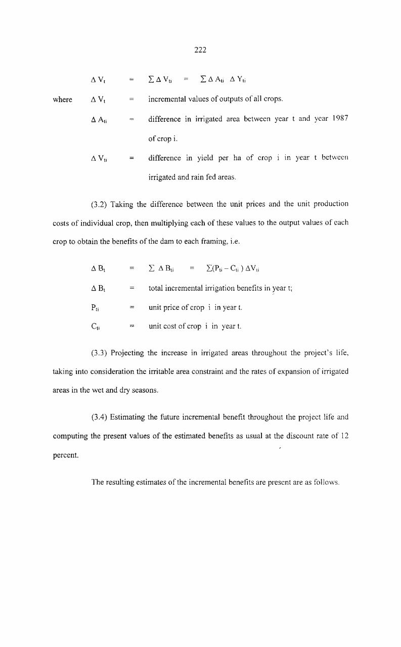
where

222

incremental values of outputs of all crops.

difference in irrigated area between year t and year 1987

of crop i.

difference m yield per ha of crop

irrigated and rain fed areas.

m year t betVv'een

(3.2) Taking the difference between the unit prices and the unit production

costs of individual crop, then multiplying each of these values to the output values of each

crop to obtain the benefits of the dam to each framing, i.e.

total incremental irrigation benefits in year t;

unit price of crop i in year t.

unit cost of crop i in year t.

(3.3) Projecting the increase in irrigated areas throughout the project's life,

taking into consideration the irritable area constraint and the rates of expansion of irrigated

areas in the wet and dry seasons.

(3.4) Estimating the future incremental benefit throughout the project life and

computing the present values of the estimated benefits as usual at the discount rate of 12

percent.

The resulting estimates of the incremental benefits are present are as follows.

223

Based on the previous plan and estimates in the feasibility report, the planned

irrigation benefits were estimated at about 199.0 million bahts per year (1980 constant

price), depending on the time required for full agricultural development. Hmvever. with the

update values of economic farm gate price for paddy and estimated implementation

schedule of the irrigation project reflecting the current progress it is estimated that the

optimistic estimated of the planned irrigation benefit, is 2,064.14 million bahts (1996

constant price). And the beneficial estimate of the irrigation water is about 0.06 bahts per

cubic meter.

3.3 Water Supply

3.3.1 Objective

The major objectives of studying the water supply aspect are to present the

existing water supply conditions, and to assess benefits of all downstream water supplies,

including water supplies for domestic and industrial water uses and for salinity intrusion

control.

3.3.2 Methodology

Data on water supply were obtained from literature review as well as from data

collection from different concerned agencies including the Provincial Water Works

Authority (PWA), the Health Department and Surat Thani Water Works. The last office

was also visited during field trip to gather additional data on its operation and on water

quality of the Phun Phin raw water. Projection of population growth was carried out based

on the data collected from different sources including the National Economic and Social

development Board (NESDB), and that future water demand was undertaken based

224

partially on the previous study of Public Work Department. Review of the surface water

hydrology study related to the Rajjaprabha project was also conducted to obtain the data

needed for evaluation of probable effects, including the parts relating to reservoir operation

and downstream flow regulation.

3.3.2 Previous Study

In the EEl report, (Team Consulting Engineers Co. Ltd. 1980) the total demand

for water supply for Surat Thani municipalities was expected not to exceed about 1.2 ems

by the year 2000. Since this constituted only slightly more than I percent of the long term

average flow at Surat Thani no separate inclusion of this demand was made in the reservoir

operation studies. Maximwn flow requirements below the Rajjprabha diversion dam have

not been established. But more detailed study was found in the project report. It presents

the status of water supply in the Phum Duang river basin in the pre-dam period. Projections

for growth in population and water demand were also given. The population growth rates

for Surat Thani were estimated to be 4.5 percent per annum. The total \vater demand for

Surat Thani forecast for the year 1996, 2000 and 2005 were about 25, 28, 31 mcm per

annum, respectively. The forecast was very close to the maximum of 1.2 ems for the year

2000 as estimated in the previous study.

As for the minimum flow requirement, the recommended value for the lower

reach of Khlong Saeng river was 44 mcm per month, which is the recorded minimum Om\'

at Rajjaprabha dam site.

225

3.3.3 Result of the study

(1) Projected Population

The projected population for the entire Surat Thani province is shown in Table

6.8. The population in the urban area is about 0.992 million by year 1995. While the

population in the rural area is approximated about 0.297 million for the year 1995.

TABLE 6.8

PROJECT POPULATION IN SURAT THANI AND fN PI-IUM DUANG RURAL ZONE

Annual Growth Area 1995

Rate (%)

Surat Thani Province (total) 3.27 992,516

Phum Duang Rural Zone 297,755 -

(Approx. 30 % of provincial total)

Source Surat Thani Provincial Office

(2) Water Supply Status

Water supply in Phum Duang river basin can broadly be classified into two

categories i.e., urban and rural.

(2.1) Urban \Vater Supply

At present, urban water supply 111 Surat Thani are managed by the local

municipality and are supported technically by the provincial Water Supply Division of

226

Public Works Department (PWD). Consideration is being made to transfer the

management and operation of the water supply systems to the Provincial Water works

Authority (PWWA). The total water consumption in urban area (Surat Thani municipal

and Phun Phin district) is about 6.07 mcm in the year of 1995 as sho\vn in Table 6.9.

(2.2) Rural Water Supply

Rural areas of the Surat Thani province (Khlong Phum Duang Rural zonc)

have relatively low population density. Also rain, surface water, and ground water are

plentiful here and that represent convenient Sources for rural water supply. As a result

there are only few rural water supply systems in this area. The total watcr consumption in

rural zone is about 5.22 mcm for the year of 1995 (Table 6.9).

(3) Future Demand for Water Supply

Future water demands was estimated taking into account growth in population,

industry, and developments in tourism sectors in Surat Thani. Major industries in Surat

Thani are rice mills, fabrication plants, and engine repair shops. Earthenwarc home

industry found in Surat Thani consumes only small amount of water. The demand for

water form miscellaneous industries estimated at about 12 percent of domestic water

demand in the urban areas. Majority of industries are related to agricultural and fisheries

production ceramics, earthenware, wood, electronics and electrical products. An industry

complex is under implementation in Surat Thani. It is located on 2,500 rai on the eastern

side of Surat Thani. Water supplies for this complex are planned to be from the Phul11

Duang river. Based on the planned production target for each type of industry and its

corresponding water consumption rate, the Surat Thani Water Supply Division of Surat

227

Thani municipality has estimated the potential water demand for this complex at ],000

m3/day, or 1.09 mcm/year.

The construction of infrastructures was scheduled for completion by the end or

1990, the full water demand is conservatively estimated in 1995.

Demand for water with respect to tourism was estimated from the number of

hotel rooms. At present there are 46 hotels with a total of 1,850 rooms. Capacity of these

hotels is judged adequate up to 1995. After 1995 and increase of 150-250 rooms per year

were assumed for Surat Thani province. Based on the future development described abov~,

the following criteria are assumed for estimating future water demand:

(a) Per capita consumption of 100 litres per day per person for the year 1995-

1999, 11 0 litres per day per person for 2000-2004, 120 litres per day for

2005-2009, and 130 litres per day per person in the year 2010 for urban

area in Surat Thani.

(b) Per capita consumption of 80 litters per day per person for the year 1995-

1999, 90 litres per day per person for 2000-2004, 100 litres per day per

person for 2005-2009, and 110 litres per day per person in the year 2010

for rural area; and

(c) 1.2 m3 per day per room for hotels including services and supporting

facilities.

The annual water demand from Phum Duang river will increase from 12.42

mcm in the year 1995 to 28.84 mcm in the year 2010 as shown in Table 6.10.

228

TABLE 6.9

WATER CONSUMPTION IN SURAT THANI MUNICIPALITY - PHUN PI-ITN AND

KHLONG PHUM DUANG RURAL ZONE (1995)

Community 1995

Urban

Domestic Uses

Population served (No.) 125,300

Consumption rate (litres/person/day) 100

Water demand 4.57

Indust~ Uses

Water demand 0.55

Tourism Uses

No. of room 1,850

Consumption rate (litres/person/day) 1.2

Water demand 0.92

Sub total 6.07

Rural Area

Population served 60 % of the total (No.) 178,653

Consumption rate (litres/person/day) 80

Water demand 5.22

Total 11.29

Total consumption + 10 % loss, m3/yr 12.42

Source: Estimated by 1. Kruger A/S consulting Engineers in Master Plan and Feasibility

Report.

229

TABLE 6.10

PROJECTION OF FUTURE WATER DEMAND (1995-20 10)

Water Demand (mem)

Community

1995 2000 2005 2010

Urban

Domestic Uses

Population served (No.) 125,300 162,000 202,SOO 264,000

Consumption rate (day/person/day) 100 110 120 130

Water demand 4.S7 6.50 8.87 12.53

lndustr): Uses

Water demand 0.S5 0.78 1.07 1.51

Tourism Uses

No.ofroom 1,8S0 2,850 3,850 4,850

Consumption rate (day/person/day) 1.2 1.2 1.2 1.2

Water demand 0.92 1.25 l.70 2.13

Sub total 6.07 8.58 11.63 16.17

Rural Area

Population served 60 % of the total (No.)

Consumption rate (day/person/day) 178,653 209,836 226,540 250.200

Water demand 80 90 100 110

5.22 6.89 8.27 10.05

Total 11.29 15.42 19.90 26.22

Total consumption + 10 % loss, m3jyr 12.42 16.96 21.80 28.84

230

(4) Water Demand for Salinity Intrusion Control

Controls of salinity intrusion into the Phum Duang river are the objective of the

studies. The amount of fresh water flow and required for this purpose is estimated from the

relations of fresh water flow salinity intrusion established in this study. The objective is to

control salinity concentration at 250 ppm or 0.25 ppt at a distance 5 km from the river

mouth. The fresh water flows required for this are 5.4 m3!scc and 3.5 m3/sec for the high

water slack and to floor the rising tide condition, respectively. Hence 5.4 m3;sec or about

15 mcm/month is the fresh water flow required for control the salinity intrusion.

(5) Water Supply Benefits

The water supply benefit is estimated based on the cost of having alternation

source for the planned water supply systems, which depend on raw water from the Phum

Duang river. Benefit from the use of water from Phum Duang river as raw water for eater

supply systems along the river is assessed from the cost of the ground water alternative

source. The present worth value (1996 price level) of raw water from the Phum Duang

river during the years from 1987 to 2037 for domestic, industrial and other miscellaneous

uses is estimated at about 140 million bahts or about 0.56 baht per cubic meter.

Limiting salinity intrusion at a location 5 km upstream from the river mouth is

anticipated to enhance utilization of the river watcr in the vicinity of Surat Thani town.

With the salinity intrusion control, the Surat Thani municipal water supply system can

safely draw its raw water from the river. Salt-water encroachment problems in the coastal

agricultural land along the river reach can rely better on the river water for purposes like

domestic earthenware industry. Although monetary value of thcse benefits, from salinity

intrusion control is rather small compared to other benefit, significant positive impacts on

socio-economic of residents in the estuarine communities can be expected.

231

4. TRANSPORTATION AND NAVIGATION

4.1 Introduction

Transportation system is very essential for development. In the southern region

roads have been sufficiently provided. The length of roads provided per unit area of land in

this region is greatest in comparison with other regions of the country. In 1980, the total

length of highways was reported to be about 4,800 km. Generally, the traffic is low here

with an average traffic volume of about 1,500 vehicles per day. But in Hat Yai the traffic is

the heaviest, (over 3,600 vehicles per day).

Navigation along the whole reach of the Phum Duang river is limited. The EIS

study showed that only small number of people used waterways for communication and

transportation. Relatively small numbers of motor boats were used in the vicinity of Ban

Ta Khun and Khirirattha Nikhom district.

4.2 Objective

The objective of this study is to evaluate the existing situation of transportation

and navigation, in order to assess changes induced by the implementation of Rajjaprabha

project. Beneficial impact will be quantified for subsequent use in the environmental

impact evaluation.

4.3 Methodology

The study is carried out by reviewmg all data available from variOUS

government agencies and from other related studies. Additional data were obtained from

field observations at various stations on main roads in Surat Thani. The navigation data

were also obtained from field observation in various parts of the river.

4.4 Result of the study

4.4.1 Land Transportation

The present condition of land transportation in Surat Thani was assessed from

the data obtained from field observations. These data include: vehicle composition.

average daily traffic volume (ADT), and peak traffic volume. Moreover, the data on traffic

volume on main highways in the project area recorded by the Highway Department from

the year 1985 to 1996 were used for assessing in changes induced by the Rajjaprabha

project.

(1) Present Traffic Condition

(1.1) General Description

The traffic assessment of main highways in Surat Thani was undertaken

primarily for estimating the present traffic condition in relation to those previously

investigated. Traffic counts were made on 17and 18 May 1997. The stations were selected

at the main road entering and leaving the towns of Surat Thani. Traffic counts were

performed during 7.00-19.00 hr. All four stations were counted during the same period of

time. The roads are two-way flow, asphaItic concrete pavement with an average width of

about 3 m per lane. The vehicle types are classified as follows:

Motorcycles (MC)

Passenger car (PC)

Light bus (LB)

Heavy bus (HB)

Light truck (LT)

Heavy truck (HT)

Other

- pri vate passenger cars and tax is.

- minibuses and modified pick-up trucks for

passengers with two long parallel benches.

- buses with more than 20 seats.

- trucks and pick-up trucks.

- 6 wheel and 10 wheel trucks and trailers.

- non-motorized vehicles, mainly bicycles and tricycles,

which are nomlally modified from bicycles.

(1.2) Vehicle Composition

Results of this investigation revealed that motorcycles were widely used in the

areas, this forms about 50 to 60 percent of the total number of vehicles observed. Pick-up

trucks were found to be about 15-20 percent of the total, vehicles. These are mainly used

for transporting material for commercial purposes. Passenger cars including taxis

constitute about 10 percent, with an almost equal share. Heavy trucks and lights buses \\'cre

account for about the same percentage as in the case of passenger cars. Heavy buses and

other (non-motorized vehicles) account for only less than 5 percent, except in the lov.,'

traffic area of Ban Ta Khun district where bicycle percentage was found to be a little

higher than in other places. The average percentage of traffic composition as shown in

Table 6.11. The details of vehicle composition found on working days and holidays,

respectively. The peak traffic was observed at 8.00-9.00 hr and 17.00-18.00 hr.

234

TABLE 6.11

AVERAGE PERCENTAGE OF TRAFFIC COMPOSITION ON 15,16 MAY 1997

Notes

Station

Station 1

Station 2

Station 3

Station 4

Station 1

Station 2

Station 3

Station 4

MC PC LB HB LT HT Other

106.8 58.2 87.5 22.8 38.4 39.6 17.4

88.6 32.7 68.5 17.1 26.4 24.8 1l.5

69.2 25.3 37.0 9.8 10.6 15.7 6.3

27.2 8.2 14.5 l.8 5.4 6.8 2.6

The route of Muang District to Ph un Phin district

The route of Phun Phin district to Khirirattha Nikhom district

The route of Khirirattha Nikhom district to Ban Ta Khun district

The route of Ban Ta Khun district to Rajjaprabha dam

(1.3) Average Daily Traffic Volume

In the absence of 24 hour count, average daily traffic volume (ADT) arc

estimated by adopting a criterion that vehicle flows during 10 hour count (07.00-17.00 hr.)

represent about 70 percent of daily traffic volume (Sinclair & Associate, 1983).

Comparison is also made with the ADT calculated from peak hourly flow, which is taken

as 8 percent of the daily traffic. Numbers of vehicles are converted into number of cars by

equivalent factors before calculating the ADT. The factors used are the same as those used

in EEL report, i.e., 2.5 for HB and HT, 0.25 for MC and others, and 1.0 for the rest of

them. Results of ADT calculation are shown in Table 6.12.

TABLE 6.12

AVERAGE DAILY TRAFFIC VOLUME

ADT ADT estimated Traffic volume

From 10 Ius, Hourly Peak estimated 07.0-17.0

Station From peak count

In Out In Out In Out In Out

Station 1 181.25 175.50 2265 2,194 1,396.75 1500.50 1,995 2,144

Station 2 247.25 322.75 3,091 4,034 2,035.50 2,279.75 2,908 3,257

Station 3 125.25 96.75 1,250 1,385 1,630.50 1,786.75 1,530 1,460

Station 4 56.00 60.25 700 753 391.25 431 559 616

Notes Station 1 : The route of Muang District to PhUll Phin district

Station 2 : The route of Phun Ph in district to Khirirattha Nikhom district

Station 3 : The route of Khirirattha Nikhom district to Ban Ta Khun district

Station 4 : The route of Ban Ta Khun district to Rajjaprabha dam

Source: Highway Department

It is found that the ADT values estimated from both bases are very close, in

the order of 2,000 to 4,000 for Muang Surat Thani and Phun Phin stations. At Khirirattha

Nikhom and Ban Ta Khun stations the ADT is wound to be lower, at least than l,OOO.

The average ADT at the counting station in this investigation are summarized

in Table 6.13

236

TABLE 6.13

AVERAGE DAILY TRAFFIC FROM FIELD INVESTIGATION

A verage Daily Traffic

Station

In Out Average

Station 1 2,644 2,646 2,636

Station 2 2,532 2,539 2,536

Station 3 1,236 1,246 1,240

Station 4 798 794 796

Source Survey data

(1.4) Peak Volume to Capacity Ratio

Volume to capacity (V/C) ratios are calculated from the basic capacity of 1,300

vehicles/hr (Sinclair. 1983). On this basic V/C ratios exceeding 1.0 arc possible, and in

practice may be as high as 1.5 or 1.6. However, V/C greater than 1.0 \vould limit the

vehicle speed to not exceeding 20 to 25 km/hr. The interpretation of traffic condition from

the value of V IC ratios are as follows:

VIC ratio

Less than 0.7

0.7 to 1.0

1.0 to 1.4

Traffic Condition

satisfactory

moderate to high congestion, general not satisfactory.

very low level of service road operates near practical

capacity

1.4 or more

237

extensive queues and delays, road at practical

capacity with existing traffic composition

(1.5) Peak Hour Capacity

Adequacy of existing road capacity can be assessed by comparing nominal

road capacity with the maximum one-way now record over any hour. The road capacity is

taken as 1,300 vehicles/hour/lane. The V/C ratios of less than 0.7 are considered

satisfactory and 0.7 to 1.0 as congested. The results obtain from this study show the V IC

ratios of less than 0.7 even during peak hours as shown in Table 6.14. Therefore the

present traffic condition are still under the road capacity.

(2.) Growth of Traffic Volumes

The growth of traffic volumes is used as an indicator for evaluating the impacts

from the project implementation on traffic conditions. Past records on traffic volumes

obtain from the Highway Department are used in this evaluation.

The ADT values of route No. 401 at various station along the highway from

Surat Thani to Phang-Nga vary considerably. For example, in 1995 the ADT varied from

highest of 2,460 to the lowest 618, which was about four times in magnitude. The ADT

between Phun Phin to Ban Ta Khun district recorded by the Highway Department was found

a little higher than the values obtain from this study. Major increase in traffic volumes all this

section of highway can be observed from the year 1980 to the present. Part of this may result

from Rajjaprabha dam implementation. But no significant increase has been observed from

other sections of route no 401. The impact of Rajjaprabha dam on land transportation, as

judged from the presented traffic information, can not be conclusive as this stage.

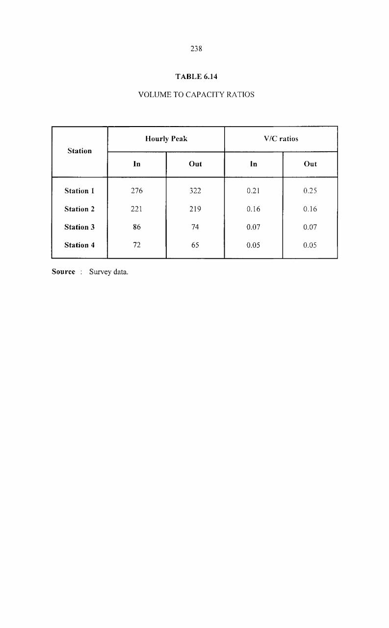
238

TABLE 6.14

VOLUME TO CAPACITY RA TIOS

Hourly Peak vie ratios

Station

In Out In Out

Station 1 276 322 0.21 0.25

Station 2 221 219 0.16 0.16

Station 3 86 74 0.07 0.07

Station 4 72 65 0.05 0.05

Source Survey data.

.,.

.,.

• s

/ )

r

./

239

/ / "

FIGURE 6,2

,.. - ._------_ .. .,.

...-~"~L_ .. " .

• ",pj101 1(0 ~9A(fGft

'"

GUl,r OF fHAIl,AND

" >, 0

+'.. • " #,

PawlS SwrfOct ~(lOCI

U~~ '-tl "'to_her R~oo;l

A.qO R.CI04I

U~d"~"f1.lC;r.,.,.

R(Wtood

0'I01'lQ"'O~ eoVtdOrt

Hlqhwoy,,",OftlttWll'I(;t Stol.OI'I

Cho",<!"ot

A ..... ~ot,l<l4"9 A.m"l1~

Ban IV,lloc;J_1

. "... b::c:= 1 ~\,' ."== .. '0 .... _.; • .,0=="" .. _=.0..: ... "

ROAD NETWORK IN SURA T THANI

240

4.4.2 Navigation

The present condition of navigation is assessed by field observation in three

parts of the river, viz:

(a) The reservoir.

(b) The upper reach downstream from Rajjaprabha dam; and

( c) The lowers reach.

(a) Navigation in the reservoir

Field observation was made in the Rajjaprabha reservoir in May 1997. Many

types of boats were observed then. They were used mostly for fishing. In non-fishing period,

boats were also used for transportation among villages located along the reservoir rim.

(b) Navigation in the Upper Reach

Observations were made at Ban Ta Khun district and Khirirattha Nikhom

distict for a period of 6 hours. During the observation 32 boats were found sailing among

the villages and both district above mentioned.

(c) Navigation in the lower reaches

More navigation activities were observed in the lower river reach downstream

from Phun Phin district to river mouth and from river mouth to the sea. Most of the boats

observed were transporting articles for fishermen households and boats for sea fishing.

241

Boats sailing along the river in the section between the river mouth and Phut)

Phin district were also counted at two hours interval. During 10.0-12.00 hours 154 boats of

all types were found sailing to and from the river mouth, respectively (See Table 6.15).

TABLE 6.15

NUMBER OF BOATS COUNTED AT SURAT THANI FISHERIES STATION

DURING 2 HOURS PERIOD

Number of boats

Type of boat

Phun Phin to River mouth To the sea

Small 69 t 17

Medium 18 12

Large 11 25

Total 98 54

Source Survey data

242

4.5 Conclusion

The situation with respect to transportation and navigation was updated ill

order to assess possible changes due to the development of Rajjaprabha dam and its

downstream project. The land transport systems, both at the regional and local level, are

found to be adequate for supporting development in the basin. The implementation of the

Rajjaprabha project has induced no material change in traffic load to the land transport

system, except during the project construction. However, better road accessibility has been

provided for rural resettlement villages.

Improved navigability is provided in most of the river reaches, both upstream

and downstream from the Rajjaprabha dam, by its flow regulation. However, this

improvement has so far not any caused significant increase in water transport in the river.

And the anticipated navigation benefit in the pre-irnpoundment environmental study has

not yet been realized.

243

5. HYDRO POWER PRODUCTION

5.1 Introduction

Hydropower system for hydropower production at Rajjaprabha dam consists of

(a) Rajjaprabha reservoir with 5,639 mcm capacity;

(b) Powerhouse with three 80 MW generating units; and

( c) 230 kv and 115 kv transmission system of 50 km length to join the

southern grid at Surat Thani substation in Surat Thani province.

5.2 Objectives

The main objectives of this study are:

(a) To estimate hydropower production benefits in term of the cost of using

alternative sources or sources of equivalent power generation;

(b) To provide beneficial estimates of hydroelectric generation per kWh to

residential, industrial, commercial, service and communication;

(c) To assess damages due to lack of hydroelectric power in a minute and a day.

5.3 Methodology

The study has been carried out based upon the review and evaluation of

existing reports and documents prepared by EGA T related to the hydroelectric

development of the Rajjaprabha dam and the region.

In order to fulfill the above objectives the following tasks are identified.

244

(1) Conventional Estimation of Hydropower Benefit:

This represents an estimate of monetary value of the electricity (power and

energy) from the Rajjaprabha powerhouse, in terms of the cost of using alternative sources

(or the next cheaper source) of equivalent power generation, so that it will satisfy objective

(a) mentioned above.

(2) Beneficial estimates of power generation of various sector's:

To fulfill the objective Cb) different investigations are needed mainly to

identify users and characteristics ofload and power market of the generated electricity

(3) Assessment of damages due to lack of hydroelectric power:

The damages under this study aspect concern both financial damages and

economic implication of the electricity supplied to various sectors of users. The lack of the

normally supplied electricity is likely to give rise to consequential damages to the various

users at different degrees.

5.4 Previous Power Facilities in Southern Region

5.4,1 Power Supply System

The power supply system in southern Thailand (EGA T' s Region 3) is shown in

Figure 6.2 The power plants available in the EGA T' s Region 3 consisted of seven power

plants. Of the seven power plants, three were oil-fired, one was lignite-fired, and three

were diesel-fired. The total installed capacity was 197.6 MW of 21 units. In Surat Thani,

245

there were three gas turbine units and one oil-tired unit totaling 75 M\V located in Phull

Phin district.

According to the EGA T' s Region 3 generation records from the 1973 to 1978

fiscal years, the average increases in power and energy demands were 19 and 18 percent,

respectively. The load forecast has been revised currently which included the PEA

development programme in southern provinces in the consideration. Accordingly, the

power and energy requirements in the 1990 fiscal year were 598 MW and 2,978 GWh,

with the yearly load factor of 57 percent.

5.4.2 Alternative of Thermal Power and Rajjaprapha Power Plant Economic

The feasibility study of the Rajjaprabha project considered the alternative

thermal plants in comparison with the installation of Rajjaprabha power plant. With the

consideration of the role of Rajjaprabha project, the combination of oil fired and gas

turbines are assumed to be a suitable alternative.

In Stage I, when the Rajjaprabha project operated with a plant factor of about

0.5, the most appropriate combination was 80 MW oil fired working at a plant factor of

0.74 and a 40 MW gas turbine working at a plant factor of 0.05

In the Stage Il, an additional unit of 60 MW gas turbine was installed to

resemble the peak generation character of the hydropower plant. The characteristic of these

combined power plants was an 80 MW oil fired working at plant factor 0.69 and a 160 gas

fired working at plant factor 0.05.

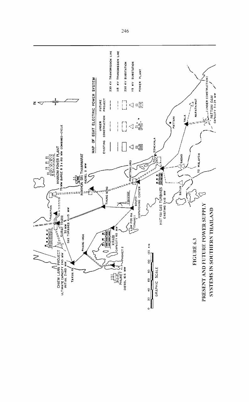
o

(;;

~)

)'1

\\

l-)

.fli

\ n

Rn

_

__

_ t

o;"

__

f .I

...

....

....

....

..a.

.. ~~! ...

1\ P

HU

NP

tllN

C;:

:,J "J{i

~·'-lr:·

.!r:~

!\ ~

_.r-~

~\ \

~t7i~:

:·::..

c::OJ~

:~L

CH

IEW

LA

RN

P

RO

JEC

T ;:

'( --

;.~~

-..... -

-"S

----

-.;,

ir K

HA

NO

M P

OW

ER P

LA

NT

U

LT

IMA

tE C

AP

AC

ITY

2

40

M

W J~Lf-

SU

RA

T T

AN

I -----

l: 7

!! M

W B

AR

GE

6

! 1

18

0 M

W

CO

MB

INE

D-C

YC

LE

INIT

IAL

2

16

0 M~{

3D

MW

'\

11

\

I G

AS

T

UR

BIN

ES

<

4.15

M

W

I:

TA

KU

A P

I.

~:, It

••

11 ~

" Ji

!'!!L

N

AK

HO

N S

RI

TH

AM

MA

RA

T

I, "

,.1~

..

DIE

SE

L

2 M

W

N ~Ir

:...2': .-;."

M

AP

O

f E

GA

T

EL

EC

TR

IC

PO

WE

R

SY

ST

EM

I \I

I U

I'IO

£R

FU

TU

RE

" .,.

EX

IST

ING

C

ON

ST

RU

CT

ION

P

RO

JEC

T

TH

UN

G ~'NG

.\

23

0 K

V

TR

AN

SM

ISS

ION

L

lN(

I, " " '.,

II!!

K

V

TR

AN

SM

ISS

IOI'I

L

INE

0 r'-

',

,---,

L._

. ...i

I I

23

0 r

<v

SU

BS

TA

TIO

N

'----'

6.

, ,.

.. \ J.'

_"i

II!!

r<

V

SU

BS

TA

TIO

N

L . .

..:.. r-: -

• ,-,

~

Gc';)

rc'::

':J"')

P

OW

ER

P

LA

NT

=

.

~!~' ..

I c.

'."')

' L

__

J

20

4

0

60

8

0

\00

1

20

!<;M

~

-J ~

GR

AP

HIC

S

CA

LE

EX

IST

ING

:3~(I:;

MW

:-

_-

I , \

G SATUN

i; \\;

.jSAD

AO

M---,

,,"")

~.--

..... _-

-~

/., \,

('-'

\~ --

.,.'\

"--"

'\ "

.\

-. ..\ \

' I

NA

RA

TH

IWA

T

'\] ,\0

MA

lAY

SIA

\

It. ,/

.-

-..

. \l

PR

ES

EN

T A

ND

FU

TU

RE

PO

\VE

R S

UP

PL

Y

') r~'

( "'t

.-. -(

UND

ER

CO

NS

TR

UC

TIO

N)

SY

ST

EM

S I

N S

OU

TH

ER

N T

HA

ILA

ND

i -

-j.,'

; P

AT

TA

Nf

DA

M

.I ~

; C

AP

AC

ITY

3

I 2~

MW

/'

\

PA

TT

AN

I

FIG

UR

E 6

.3

t-J

~

0-,

The main characteristics of the alternative plants are summarized below

Installed power (MW))

Oil fired unit

Gas turbines

Generating Energy (GWh)

Oil fired unit

Gas turbines

Plant factor (average)

Oil fired unit

Gas turbines

Stage I

120

80

40

537,5

520.0

17.5

74%

5%

Stage n

240

80

160

553,7

520.0

33.7

74 %

5%

These alternative thermal plants were used to determine the benefits of the

Rajjaprabha dam on power production.

5.4 Results of the study

Potential for hydropower production at the Rajjaprapha power plant has been

re-evaluated using the reservoir operation simulation technique, and also adopting the

revised performance characters of the hydropower generating facilities along with 25 years

actually observed reservoir monthly inflows. According to the revised estimate an average

annual energy generation of about 554 GWh can only be expected when there is water

constraint on the reservoir operation.

248

5.4.1 Power System

Ever-increasing load in EGA T southern region has resulted in a much

improved electrical power system from the pre-impoundrnent condition. Pmver and energy

demands have increased at a much higher rate in the post-impoundment period. As a

consequence EGA T has constantly been working on continual improvement and

development of its power system.

Rajjaprabha power generation provides three major contributions to the power

system III the EGAT southern region, namely energy, power, and system operation

flexibility and reliability. When the plant started its operation at full potential during 1987

to 1996 period, the average annual energy was about 554 GWh. This was approximately 28

percent of the energy demand of the whole southern region during the same period. The

peaking power of the Rajjaprabha plant also provided significant contribution to the peak

demand in the southern region, especially for the area of Phan-nga province. It provided

about 31 percent of the peak demand during 1995-1996. Providing peaking power, quickly

low maintenance requirement and a marked flexibility and reliability to the EGA T power

system are the advantageous abilities of the Rajjaprabha power plant.

5.4.2 Conventional Estimation of Hydropower Benefit

The stream of benefits expected to be obtained from the dam are summarized

in table 6.16, While the stream of investment and operation cost are presented in Table

6.17. The overall project (included power, irrigate and fishes) evaluation shown the B/C

ratio of 1.60 while the internal rate of return is 16.2 percent. A sensitivity analysis was

249

made considering the power benefit alone; the internal rate of return of 14.68 while the

B/C ratio of 1.44 at 10 percent interest rate were obtained.

TABLE 6.16

BENEFIT FLOW OF RAJJAPRABHA PROJECT

Year Benefits (in Million Baht)

Year Benefits (in Million Baht)

Invest. O&M Fuel Invest. O&M Fuel

1 0 0 0 26 123.00 58.00 681.00 2 53.00 0 0 27 102.00 606.00 704.00 " 107.00 0 0 28 107.00 626.00 724.00 j

4 213 .00 0 0 29 213.00 642.00 747.00 5 303.00 0 0 30 229.00 661.00 769.00 6 552.00 0 0 31 650.00 681.00 792.00 I

7 164.00 29.00 273.00 32 484.00 704.00 815.00 8 0 36.00 353.00 33 148.00 724.00 841.00 I 9 0 36.00 362.00 34 0 747.00 864.00

10 0 36.00 372.00 35 0 726.00 890.00 11 221.00 36.00 384.00 36 0 58.00 916.00 12 369.00 36.00 396.00 37 0 58.00 945.00 13 148.00 36.00 408.00 38 0 58.00 973.00 14 0 58.00 470.00 39 0 58.00 1,002.00 15 0 58.00 492.00 40 0 58.00 1,032.00 16 0 58.00 509.00 41 0 58.00 1,063.00 17 0 58.00 522.00 42 0 58.00 1,095.00 18 0 58.00 538.00 43 0 58.00 1,128.00 19 0 58.00 554.00 44 0 58.00 1,160.001 20 0 58.00 571.00 45 74.00 58.00 1,196.00 21 0 58.00 587.00 46 123.00 58.00 1,232.00 I 22 0 58.00 606.00 47 49.00 58.00 1,270.00 23 0 58.00 626.00 48 0 58.00 1,307.00 I 24 0 58.00 642.00 49 0 58.00 1,347.00 25 74.00 58.00 661.00 50 0 58.00 1,388.00

Source: EEl report

250

TABLE 6.17

COST FLOW OF RAJJAPRABHA PROJECT

Costs (in Million Baht) Costs (in Million Baht) Year Year

Civil. Elmec. Trans. Civil. Elmec. Trails.

1 56.00 0 0 26 30.00 15.00 5.00 2 76.00 0 0 27 30.00 15.00 5.00 ...,

396.00 45.00 21.00 28 30.00 135.00 14.00 -' 4 890.00 120.00 3.00 29 30.00 197.00 40.00 5 1,007.00 182.00 92.00 30 30.00 163.00 113.00 6 338.00 148.00 158.00 31 30.00 39.00 20.00 7 130.00 46.00 27.00 32 30.00 15.00 5.00 8 29.00 10.00 5.00 33 30.00 15.00 5.00 9 29.00 10.00 5.00 34 30.00 15.00 5.00

10 29.00 10.00 5.00 35 30.00 68.00 5.00 11 36.00 83.00 5.00 36 30.00 105.00 5.00 12 46.00 100.00 5.00 37 30.00 115.00 5.00 13 35.00 110.00 5.00 38 30.00 15.00 5.00 14 30.00 15.00 5.00 39 30.00 15.00 5.00 15 30.00 15.00 5.00 40 30.00 15.00 5.00 16 30.00 15.00 5.00 41 30.00 15.00 5.00 17 30.00 15.00 5.00 42 30.00 15.00 5.00 18 30.00 15.00 5.00 43 30.00 15.00 17.00 19 30.00 15.00 5.00 44 30.00 15.00 8.00 20 30.00 15.00 5.00 45 30.00 15.00 60.00 21 30.00 15.00 5.00 46 30.00 15.00 55.00 22 30.00 15.00 5.00 47 30.00 15.00 12.00 23 30.00 15.00 5.00 48 30.00 15.00 5.00 24 30.00 15.00 5.00 49 30.00 15.00 5.00 25 30.00 15.00 5.00 50 30.00 15.00 5.00

Source EEl report

From the above analysis, is can be considered that in the absence of th

Rajjaprabha project the thermal plants of equal capacity would have to be installed. Wit

respect to the environmental pollution, the alternative thermal plants will result in muc

more pollution problems.

251

5.4.3 Financial Benefit of Power Generation

Electricity generated from the Rajjaprapha power plant is mainly consumed in

Phan-nga, Ranong, Pattalung, Surat Thani, Nakhorn Sri Thammarat. About half of the

energy IS consumed in Surat Thani and Nakhorn Si Thammarat. Among the users,

industrial users consume more than a half of the generated energy. Residential and small

business users consume the remaining.

(1) Benefit to EGAT

Financial benefit to EGAT from the sale of the generated electricity to

Provincial Electricity Authority (PEA). The average annual energy benefits during 1987 to

1997was about 518.42 million bahts per year as shown in Table 6.18.

(2) Benefit to PEA

Financial benefit to PEA from users for the year 1987-1997 are estimated and

shown in Table 6.19, that the financial benefit average about 685.98 million bahts/year

5.4.4 Financial Damages Due to lack of Hydroelectric Power

Monetary benefits of power generation at the Rajjaprabha plant, taken as direct

mcomes to EGA T and PEA from the sales of electricity, are described in the previous

section. Financial damages due to lack of such electricity are just the losses of such

incomes. The financial losses by EGA T and PEA would average 351 and 424 million bahts

per year respectively.

It should, however, be noted that the lack of the normally supplied electricity is

likely to give rise to consequential damages to the various users at different degrees. Such

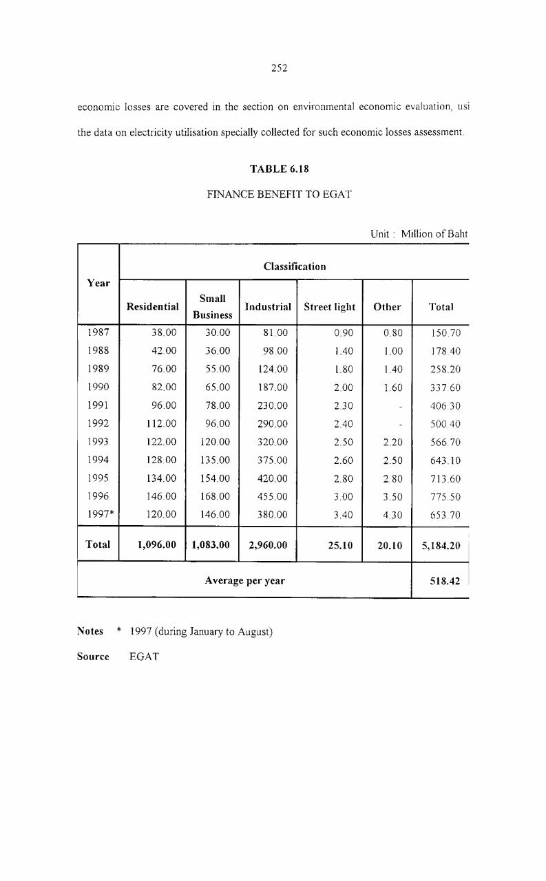
252

economic losses are covered in the section on environmental economic evaluation, usi

the data on electricity utilisation specially collected for such economic losses assessment.

Year

Residential

1987 38.00

1988 42.00

1989 76.00

1990 82.00

1991 96.00

1992 112.00

1993 122.00

1994 128.00

1995 134.00

1996 146.00

1997* 120.00

Total 1,096.00

TABLE 6.18

FINANCE BENEFIT TO EGAT

Classification

Small Industrial Street light

Business

30.00 81.00 0.90

36.00 98.00 1.40

55.00 124.00 1.80

65.00 187.00 2.00

78.00 230.00 2.30

96.00 290.00 2.40

120.00 320.00 2.50

135.00 375.00 2.60

154.00 420.00 2.80

168.00 455.00 3.00

146.00 380.00 3.40

1,083.00 2,960.00 25.10

Average per year

Notes * 1997 (during January to August)

Source EGAT

Unit: Million of Baht

Other Total

0.80 150.70

1.00 178.40

1.40 258.20

1.60 337.60

- 406.30

- 500.40

2.20 566.70

2.50 643.10

2.80 713.60

3.50 775.50

4.30 653.70

20.10 5,184.20

518.42

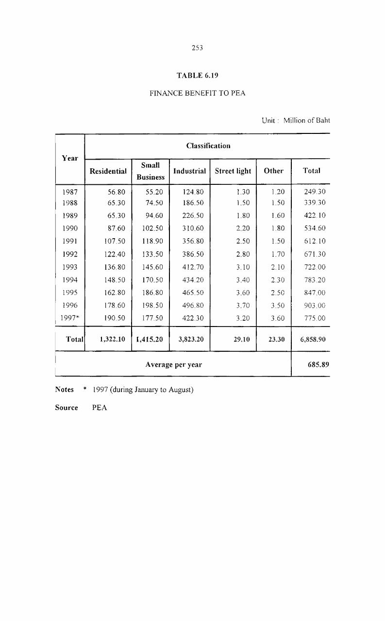
253

TABLE 6.19

FINANCE BENEFIT TO PEA

Unit: Million of Baht

Classification

Year Small

Residential Industrial Street light Other Total Business

1987 56.80 55.20 124.80 1.30 1.20 249.30

1988 65.30 74.50 186.50 1.50 1.50 339.30

1989 65.30 94.60 226.50 1.80 1.60 422.10

1990 87.60 102.50 310.60 2.20 1.80 534.60

1991 107.50 118.90 356.80 2.50 1.50 612.10

1992 122.40 133.50 386.50 2.80 1.70 671.30

1993 136.80 145.60 412.70 3.10 2.10 722.00

1994 148.50 170.50 434.20 3 AO 2.30 783.20

1995 162.80 186.80 465.50 3.60 2.50 847.00

1996 178.60 198.50 496.80 3.70 3.50 903.00

1997* 190.50 177.50 422.30 3.20 3.60 775.00

Total 1,322.10 1,415.20 3,823.20 29.10 23.30 6,858.90

I Average per year 685.89

Notes * 1997 (during January to August)

Source PEA

254

6. FLOOD PROTECTION

6.1 Introduction

Flood control is one of the major components proposed in the Phum Duang

river basin development plan. The feasibility study report gives a brief describing of past

flood events. On the basis of this flood protection strategy was planned, and a preliminary

design of the plan was proposed in the report. Later in 1980 an Environmental and

Ecological Investigation of Rajjaprabha Multipurpose Project was prepared for EGA T. In

this description on historical flood events was prescribed along with results of the

preliminary flood hydrology study. It also assessed flood control benefits and probable

environmental effects of such assess. In the update versions of the report the protection

plan proposed in the feasibility study remained unchanged. Only the quantities of

construction material and costs were revised.

6.2 Objectives

Main objective of this aspect of water resources management is to reassess

flood protection benefit using additional data and information collected up to water year

1996. To accomplish this objective the following study aspects are carried out and

presented in the following sections.

(a) Flood damage data compilation and analysis;

(b) Review of previous flood protection benefit estimations;

(c) Reassessment of flood protection benefit.

255

6.3 Methodology

The methodology employed for determining the flood control benefits was the

comparison of the flood damage condition for the case with and without the project. By

assuming that the flood damages are directly proportional flood peak magnitudes, the

relationships of flood peak magnitudes and damages are constructed at the control points

by using the available data of flood damages

Finally, the flood damage reductions or flood control benefits were then

estimate from the relationships of flood peak, flood damages and flood frequencies. These

would then be the beneficial effects of the Rajjaprabha dam reservoir on the downstream

flood damages control.

6.4 Previous Study

The previous study present some collected data on paddy damage in the crop

years of 1969-1970, 1976-1977 and 1980-1981 by systematic questioning the province and

district officers, as well as individual farmers during the field surveys. Only results of Ph un

Phin -and Ban Na San districts are available as shown in Table 6.20

256

TABLE 6.20

PREVIOUS FLOODED AREA IN SURAT THAN!

Flooded Area,(rai)

Districts

1969-1970 (Dec.) 1976-1977 (Sept.) 1980-1981 (July)

Phun Phin 597.6 612.2 587.5

Ban Na San 450 46 34

Source Surat Thani Provincial Office.

6.4 Results of the Study

The investigation indicates that the major cause of flood is the heavy storm .'

during the northeast monsoon season i.e. November through January. The river basin

upstream of Khlong Phum Duang and including the town of Phun Phin district covers an

area of 4,668 km2. About 2,960 km2 of this is the steep mountainous area above

Rajjaprabha damsite. From Rajjaprabha to Khirirattha Nikholl1 district is the rolling

hillside area of about 2,291 km2. The average ground slope of this area is considered as

moderate. From Khirirattha Nikhom district to Phun Phin district lies a vast flat paddy fIeld

of alluvium deposit. The average river bed slope above Khirirattha Nikhom district is

approximately 0.02, and decreases abruptly to about 0.025 when it enters the town of

Khirirattha Nikhom. The river bed slope becomes even flatter as it runs downstream. Such

topographic features produce streamflow of high peak and large volume, which reaches

Khirirattha Nikhom district rapidly. By rationing with the size of the catchment area, about

60 percent of total flood volume should be from drainage area above the Rajjaprabha dam.

257

6.4.1 Flood Protection Components

Before the construction of Rajjaprabha dam the river reaches downstream from

the damsite were subjected to flooding of varying severity for almost every year.

Therefore flood protection was considered as one of the main purposes of Rajjaprabha and

its downstream project development. The flood control storage provided at the Rajjprabha

reservoir and the downstream flood control system were planned to minimize, or

completely alleviate damages from all less severe flood events than the 100 year project

designed for flood control. The upstream flood protection system consists of reserved flood

control storage, varying from 135 to 217 mcm depending on the time of the year, and a

service spillway with 4,500 ems design capacity. The downstream flood protection system,

which is still being implemented, consists of: (a) flood protection dikes on both banks or

the river upstream from the diversion dam (b) service and emergency spillway of the

diversion dam ( c) flood training dike along the center main canal (d) a system of main

drains with control gates and pumping stations and (e) two orifice/flume structures for

flood flow diversions to suit downstream channel capacities.

Many components of the downstream flood protection system are presently

being implemented. According to the recent implementation plan, significant flood

protection for the Surat Thani town will be provided when the construction of stage II of

the right bank dike upstream from the diversion dam is completed in the fiscal year 1988.

Also the Ban Ta Khun town and its vicinity area will be significantly protected by the

fiscal year 1992 when the planned flood training dike along the right bank of Khlong

Saeng downstream from the diversion dam is completed. The upstream flood control

component at the Rajjaprabha dam significantly contributes to flood protection of the

258

downstream flood prone areas. On an average it provides reduction of flood peak discharge

at Surat Thani by about a half Although the planned downstream flood control component

has not yet contributed to its full potential, it has presently very significantly shortened

flood duration in the downstream agricultural area in Surat Thani. This has resulted a

marked reduction in agricultural flood damages.

6.4.2 Flood Damages Estimated

Damages in Khlong Phum Duang and Khlong Phun Phin river basin are mainly

on the paddy rice and some on the upland crops grown in the wet season. An analysis is

made in connection with thid study to determine, on a preliminary basis, the flood damages

in Phun Phin, Khirirattha Nikhom, Ban Ta Khun and Muang Surat Thani district were

collected and reviewed.

Table 6.2 I present the summary of estimated flooded areas and damages on the

agricultural production of available crop years, separated into district as Phin Phin,

Khirirattha Nikhom and Ban Ta Khun incombination and Muang Surat Thani district. The

flooded areas was shown in Figure 6.5.

TA

BL

E 6

.21

ES

TIM

AT

ION

OF

FL

OO

D D

AM

AG

ES

SE

PA

RA

TE

D O

NT

O D

IST

RIC

TS

U

nit:

M

illio

n of

Bah

t

Sep

tem

ber

1989

Ju

ly 1

990

Sep

tem

ber

1991

S

epte

mbe

r 19

92

July

199

3 S

epte

mbe

r 19

93

Flo

oded

F

lood

ed

Are

a A

rea

Pad

dy

Pad

dy

Pad

dy

Pad

dy

.....

.....

.....

......

.....

.....

en

en

en

en

en

en

Loc

atio

n 0

0 0

0 0

0 U

U

U

U

U

U

tJ

l tfJ

tJ

l en

tJ

l CI

J 0

-(1

) 0

-(1

) 0

-(1

) 0

-('.

.) 0

-Q

) 0

-Q

)

0 gp

0 gp

0 co

0

co

» 0

co

0 O

f)

» .....

»

.....

-8

.....

<"J

>.

.....

<"J

.....

('j

» .....

('

j "0

U

~

"0

U

El u

§ "0

U

§

"0

U

§ "0

U

~

"0

"0

"0

"0

"0

"0

<"J

.....

<"J

.....

('

j <"J

.....

CI

l .....

CI

l .....

CI

l .....

Q

..

Q)

Cl

Q..

Q

) C

l Q

..

Q)

Cl

Q..

('.

.) C

l Q

..

Q)

Cl

Q..

Q

) C

l -5

.s

-5

...c

..c:

-5

.....

.....

0 0

0 0

0 0

Phu

n P

hin

9955

-

6.22

99

2 -

5.83

1,

678

72

10.6

0 1,

606

598

10.9

7 -

--

1,60

0 80

0 11

.25

Khi

rira

ttha

Nik

hom

&

Ban

Ta

Khu

n *

* -

* *

-51

2 23

6 3.

67

635

209

4.29

]9

2 8

1.21

61

4 18

53

4.12

Mua

ng D

ist.

* *

-*

* -

-12

8 0.

20·

682

79

4.79

-

--

363

38

2.33

'-----_

.-.---

'--

'-..

--

-

Not

es

(1)

Flo

oded

are

a is

exp

ress

ed i

n he

ctar

e.

(2)

"Oth

er C

rops

" m

eans

fie

ld c

rops

and

veg

etab

les.

(3)

Uni

t dam

ages

cos

ts o

n ag

ricu

ltur

al p

rodu

ctio

ns a

re a

ssum

ed a

s 1,

000

baht

per

hec

tare

for

pad

dy a

nd 2

50 b

aht p

er h

a fo

r ot

her c

rops

(4)

* m

eans

dat

a ar

e no

t av

aila

ble

N

Vl

1.0

1,

(;

f',

.

( "

z ~

"~+L.

__ ::::::::

::=-

:------

..........

OBcnNO;;~Ji

r. fN

JI [

lO,,

; 0(

1:-

oB

on

No

; n

ai

o U

on

aiJ['O~ O

f

~-~.-

... -

.. ----..

_ .l

....

.. _

_ '_

' __

__

.

FIG

UR

E 6

.4

LE

GE

ND

?7~~3;

~!;;

;,~~

/.

~~z~~

:::~,>"~",,,

IP\'IIH

:Plllii

::!!

!; :!;

:;Ilil

~

FL

OO

D A

RE

A S

UB

JEC

TE

D T

O E

XC

EP

TIO

NA

L F

LO

OD

EV

EN

T P

HU

M

DU

NG

RIV

ER

BA

SIN

o 2

~

re:

r:::::

::~

; G(O"k~

Sco

le

flGn ~.nQ L

o

.. H

ug,

... "

,. ,.

Mo

c N

om

T

o P

i F

loo

d

Ro

ut;

nQ

/l

r~o

17

0 K

m2

Cro

pp

ed

L

an

ds

SU

bje

ct

10

r(h

lon

q

F~um

Du

on

g

Flo

od

inq

65

Km

2

Flo

O(!

lfH

J

ffO

ft' Kht~nQ

P"

ur.

P

hlO

u

"j

Up

SH

eOfn

CO

lc!H

tlcn

l~

55

Km

2

De\

fC) A(

~o

110

Km

2

To

Te!

f~(QC

~OO

Ktr

?

t--.J

0\ o

261

Flood damage data presented in Table 6.21 alone an: not sufficient to derive

the relationship between the magnitudes of flood peaks and damages, since the available

data are in the range of floods having low return periods. To overcome this problem, the

boundaries of the maximum extent of the area that is under threat of flood was outl ined in

the topographic map of scale 1 :50,000 to estimate the possible upper limits of the flooded

areas separated for each district. These upper limits of the flooded areas and corresponding

damages were used as additional data in deriving the relationship of the flood peak

magnitude and damage. It is estimated that the flood damages of 24.3 million baht for

Khirirattha Nikhom and Ban Ta Khun district (in combination) and 56.2 million baht for

Phun Phin district are expected to be the upper limits of damages corresponding to the

flood with the return period of 1,000 years.

Based on the available data and assumptions of flood damages described

above, the relationships of flood peaks and damages are constructed for the above

tabulated flood zones.

relation is :

For Khirirattha Nikhom and Ban Ta Khun district in combination, the derived

D 19.161 In Q - 138.808, for Q > 1,400 cms

0, otherwise

In case of Phun Phin district, the similar relation is

D = 36.405 In Q - 266.722, for Q > 1,520 ems

= 0, otherwise

D is expressed as the flood damage in million baht, Q the magnitude of flood

peak in ems.

262

As the flood frequency and flood peak relationships are already analyzed for

these control points, the transformation of flood damage and flood peak relationships, to

the flood damage frequency can be systematically carried out. These relationships, which

are expressed as the flood damage and the number of occurrence in 100 years, i.e. 100

divided by return period at control points and flood zones are presented in Figure 6.6 and

6.7 for Khirirattha Nikhom and Ban Ta Khun district, and Phun Phin district, respectively.

The area under the curve is the total flood damages expected to occur in 100

years. Hence, the existing annual flood damage, in case without the Rajjaprabha reservoir,

for each particular zone is determined by diving the total area under the curve by 100. The

estimated annual flood damages in case without the proposed reservoir are about 3.487 and

9.893 million bahts for Khirirattha Nikhom and Ban Ta Khun district, and Phun Phin

district, respectively. This represents the existing flood damage, condition of the Phul1l

Duang river basin.

-+-

L:­ a

25

20

CD

15

c ,2

~

ID

10

01

a E

a o

5 o

I I

LEGE

ND:

\ /\

...... W

ITH

RA

JJA

PR

AB

HA

RE

SE

RV

OIR

--

WIT

II R

AJJ

AP

RA

BH

A R

ES

ER

VO

IR

11 /

WIT

HO

UT

RA

JJA

PR

AB

HA

RE

SE

RV

OIR

----

WT

I1l0

ur

RA

JJA

PR

AB

HA

RE

SE

RV

OIR

~(),I

/~//

~/,

' )1

,>,

V />

. /~:V/>~

. . '"

//

,/

/

/ /"/r~

~/-:

:j/'

/ ;-:;

///~7?

>"'r"'

~ "" //,'

/ /

/ /

/./

/ /"

-

~777

~

/ "[,

.j

. /

,/ ~

/ // "

'7

. V'

/,/ / FL

OO~O

NTRO

L B

EN

EF

IT

IN

100

( AR

S ,7

; k"

//

,//./

,/,/ /

v/./

./

/ ,/

/ /

/ /

/ //"

//'

/ /"

,"

"" '"

"/'/

/ ,7

77

-//

,"

// t/

/'-:

, ~-;r t"

7-"

"/-;

.._

o 5

10

15

20

25

3

0

35

4

0

45

Num

ber

of

Occ

urre

nce

in

100

Yea

rs

FIG

UR

E 6

.5

FL

OO

D D

AM

AG

E F

RE

QU

EN

CY

CU

RV

E O

F K

HIR

IRA

TT

HA

NIK

HO

M A

ND

BA

N T

A K

UN

DIS

TR

ICT

IN

CO

MB

INA

TIO

N

50

5

5

N

0\

\..J

--.c: c ca

:E

WIT

HO

ur

RA

1JA

PR

AB

HA

RE

SE

RV

OIR

f 300

I \/7t~~·4

I i .

c o

20

0 I

J"i

/

I /

/ ,_

.J

"<o.

-<::::

I /

::V

,.. ..

10

01

'

=Sk'~~~ -l

/'''w

~~,,-'"

. I /

?-

• \

/ /.

u •

-L

' :-

o 10

IS

2

0

25

3

0

35

Nu

mb

er

of

OC

curr

en

ce

in

10

0 Y

ears

FIG

UR

E 6

,6

FL

OO

D D

AM

AG

E F

RE

QU

EN

CY

CU

RV

ES

OF

DIS

TIU

CT

-7

4

5

50

-r-_

SS

6

0

N

0\ ~

265

6.4.4 Flood Protection Benefit

Benefit of a flood protection project is naturally the reduction in nood damages

prevailing under the without project condition. Nature of flood damage characters and

flood responses of residents in the flood prone and vicinity areas indicate that the flood

protection benefit can be categorized into three types: direct flood protection benefit

indirect flood protection benefit, and benefit from more intensive utilization of lands and

properties enhanced by the flood protection.

It can be seen that the flood damage can be significantly reduced in the areas of

Khirirattha Nikhom and Ban Ta Khun district. The residual flood damages for case with

the Rajjaprabha reservoir are estimated to be 0.187 and 3.830 million bahts annually for

Khirirattha Nikhom and Ban Ta Khun district in combination, and Phun Phin district,

respectively.

The flood damage frequency curves for the selected zones, shown in Figure 6.6

and 6.7, describe the flood damage reduction to be resulted from the implementation of the

Rajjaprabha dam.

The areas between the flood frequency curves for the curves without and with

the Rajjaprabha reservoir, divided by 100, will be expected annual flood control benefit of

the project the estimated annual flood control benefits are 3.30 and 6.06 million bahts for

Khirirattha Nikhom and Ban Ta Khun district in combination, and Phun Phin district,

respectively with the total amount benefit of 9.36 million bahts. This estimated flood

control benefit is only for the reduction in flood damage on agricultural productions.

266

7. WATER POLLUTION

7.1 Introduction

The 90-km length of the Phum Duang river downstream from the dam has been

planned for multiple uses. The major water uses of interest from a water pollution control

viewpoint are:

(a) Water supply including municipal, sanitary district, self-supplied

industrial and rural domestic utilization:

(b) Water contact and non-water contact activities, e.g., bathing, fishing. and

riverside parks;

(c) Navigation; and

(d) Irrigation

To serve these multiple uses, the quality of the river water must be maintained

to meet all criteria for these water uses. In conjunction with the water use activities, the

river also receives pollution loading from various sources both directly and indirectly, c.g.,

municipal and industrial wastewater, irrigation return flow, and various non-point pollution

loading. The river itself can assimilate the pollution loads to a certain limit, and still

maintaining the river water quality. The capability of the river to assimilate waste loads

depends on various environmental factors of both the manageable and unmanageable

types, e.g., the physical and hydrological characteristics of the river, climate, and the

nature of waste loads.

The study on water pollution is, then, aimed at the preliminary identification of

major pollution sources and the consequence of water quality deterioration subjected to the

267

environmental factors, both of the manageable and unmanageable types. The study results

serve as guidelines for the planning of water quality management.

7.2 Objective and Scope

The main objective of this study is to evaluate the direct and indirect effects or

water pollution and benefits on pollution control from the regulation of water in the proj eet

implementation. The scope of the study includes the following aspects:

(a) Assessing major pollution sources, i.e., domestic wastewater, industrial

wastewater and agricultural wastewater.

(b) Evaluating the extent of pollution, then, estimation of assimilative

capacity of the Phum Duang river; and

(c) Assessing the benefits on pollution control from the regulation of water.

7.3 Assessment of Pollution Sources

The pollution loading to the 90 kilometer length of the Khlong Phum Duang

river are of three main categories: (1) domestic wastewater, (2) industrial wastewater, and

(3) irrigation return flow. Various pollution sources discharge pollution loads to river

according to their water-related activities along the river reach. During this study period no

irrigation return flow was observed due to rather limited application of the irrigation water.

7.4 Evaluation of the Pollution Sources

The evaluation of pollution sources is carried out with respect to the three main

sources, i.e., domestic, industrial and irrigation.

268

7.4.1 Domestic Wastewater

Wastewater discharges from the four communities VIZ., (i) Ban Ta Khun

district (ii) Khirirattha Nikhom district (iii) Phun Phin district and (iv) Muang Surat Thalli

district are estimated from population data and water consumption. Characters of the

generated wastewater were assessed from the samplings and analyses of wastewater

samples collected during this study. Then total domestic pollution loading, in term of

ultimate BOD loading, was estimated for the three communities to increase from about

1,760 kg/day in 1996 to about 2,530 kg/day in 2000 and to be 3.780 kg/day in the year

2005 as shown in Table 6.22.

7.4.2 Industrial Wastewater

Major sources of industrial wastewater discharges into. the Phum Duang river

are in the towns of Surat Thani. The main sources of these discharges are fishery related

and food processing industries, the fish-landing pier of the Fish Market Organization. Total

ultimate BODs loading from industry wastewater and the fish-landing pier is estimated to

grow from about 20,360 kg/day in 1996 to about 26,000 kg/day in 2000 and to be 32,480

kg/day in the year 2005 as shown in Table 6.23.

7.4.3 Irrigation Return Flow

At present negligible irrigation return flow can be expected, as the irrigation

water supply is very limited. So, pollution loading in terms of BOD from irrigation return

flow will be negligible compared to other sources. Therefore, the total ultimate BOO

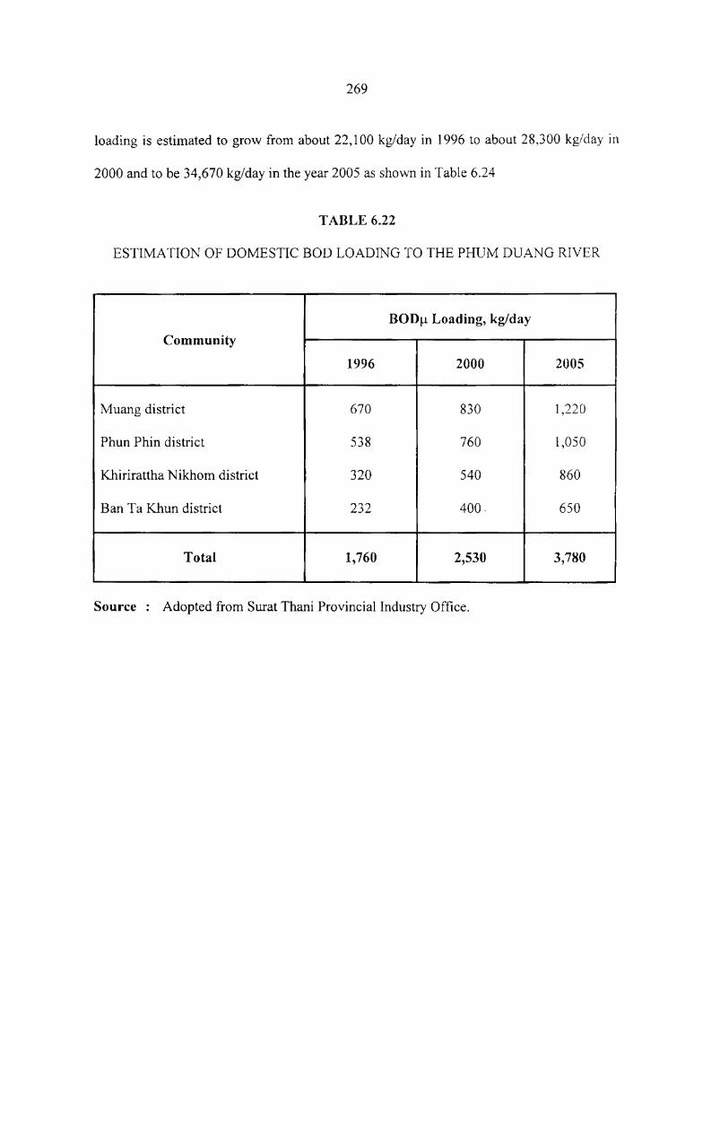
269

loading is estimated to grow from about 22,100 kg/day in 1996 to about 28,300 kg/day in

2000 and to be 34,670 kg/day in the year 2005 as shown in Table 6.24

TABLE 6.22

ESTIMATION OF DOMESTIC BOO LOADING TO THE PHUM DUANG RIVER

BODf.! Loading, kg/day

Community

1996 2000 2005

Muang district 670 830 1,220

Phun Phin district 538 760 1,050

Khirirattha Nikhom district 320 540 860

Ban Ta Khun district 232 400. 650

Total 1,760 2,530 3,780

Source Adopted from Surat Thani Provincial Industry Office.

270

TABLE 6.23

ESTIMATION OF INDUSTRIAL AND FISH LANDING PIER BOO LOADING TO

PHUM DUANG RIVER

BOD~ Loading, l{g/day

Source of Wastewater

1996 2000 2005

Industrial 1,585 3,882 4,680

Fish landing pier 18,835 22,718 27,800

Total 20,360 26,000 32,480

Source Surat Thani Provincial Industry Office.

TABLE 6.24

ESTIMATION OF BOD LOADING FROM IRRIGATION RETURN FLOW

BOD~ Loading, kg/day

Source of Wastewater

1996 2000 200S

Paddy, Crops 3,900 4,740 6,634

Livestock 18,200 23,560 28,036

Total 22,100 28,300 34,670

Source: RID

271

7.S Estimation of Assimilative Capacity of the river

Having estimated the pollution loading the waste assimilative capacity (W Ac)

of the Phum Duang river is preliminarily estimated using the Streeter-Phelps oxygen sag

equation given below.

D

where D

Do

Lo

X

U

Kd

Kr

Ka

Kd Lo --- [ exp (-Kr x/u) - exp (-Ka x/u) ] Do exp (-ka x/u)

Ka-Kr

Oxygen deficit, mg/I.

Initial oxygen deficit at the point of waste discharge, mg/l.

Ultimate BOO at the point of discharge, mg/I.

Distance downstream from the point off discharge, km.

Velocity of flow in the river, km/day

= BOD deoxygenation rate, dai)

BOO decay rate, dai)

Re-aeration rate of the river day-)

The degree of accuracy in the estimation of W AC In this study is or

preliminary level. Estimation of some parameters are based on both field data, and

information derived from literature.

Assuming a safe level of dissolved oxygen of 4 mg/l the Phum Duang river is

assessed to have adequate waste assimilative capacity for the BOD5 loading in the year

2000, provided that a minimum flow of 44 mcm/month is maintained. However, if the

minimum flow of only 15 mcm/month for salinity intrusion control is maintained the

assimilative capacity will reduce to about 8,000 kg/day. In this case the capacity will be

adequate only for the domestic loading and the wastewater from the Surat Thani fishery

port must be properly treated.

CHAPTER VII

QUALITY OF LIFE VALUE

CHAPTER VII

QUALITY OF LIFE VALUES

1. INTRODUCTION

Quality of life values are among the most important environmental resources

values with which the public is concerned in developing any kind of large-scale projects.

With respect to a large dam and reservoir development like the Rajjaprabha dam, one of

the primary concerns is that related to adverse socio-economic effects on the people which

have to be evacuated and relocated due to impoundment of water in the reservoir. This is

due to the fact that, while unaffected people would benefit from power generation, flood

protection in the downstream areas, fisheries development in the reservoir area, and the

irrigation scheme, but the existing inhabitants of the proposed reservoir will have to suffer,

at least psychologically, once they are informed of their fate in the near future.

The quality of life values which were investigated in relation to the

Rajjaprabha dam included (i) socio-economic and resettlement (ii) public health and

nutrition (iii) tourism and recreation, and (iv) archaeology and historical values. Since the

first life value is related directly with the people who has to be evacuated and resettled,

they were given the first priority. Alteration of public health, recreation, archaeological and

historical caused by the project can also be a significant environmental complication.

2. SOCIO-ECONOMIC AND RESETTLEMENT ISSUES

2.1 Introduction

The overall objective of the study is to identify the socio-economic impact

owing to the significant changes occurred after the project implementation. The study has

focussed on the resettlement and irrigation areas. In the resettlement area, emphasis has

been given to the quality of life of the farmers before and after moving into the

resettlement area and also to the means to improve the quality of life of farmers living in

the resettlement area. In the irrigation area, other comparative analysis of farm enterprises

between irrigated and non-irrigated farm groups is evaluated in order to identify benefits

from irrigation. Meanwhile, the problems confronting the farmers were also investigated.

Moreover, socio-economic structure of the people in the river basin was also investigated

to understand the overall structure of the people living in the area. This was done by

analysing the village profile.

The results of the analysis are presented in three sections viz., (i) analysis of

farm enterprises in the irrigated area vis-a-vis the non-irrigated area (ii) illustration of the

quality of life of the farmers prior to and after resettlement and (iii) summarizing the socio­

economic structure of village profile of the river basin using data from the survey of the

Community Development Department.

274

2.2 Irrigation Project

2.2.1 General Characteristics of Farm Samples

In order to evaluate the benefits from irrigation, farmers from Bang Yai village

and Tha Kham village were randomly selected and classified into two groups, namely the

irrigated group which refers to farmers who have access to irrigation water, and non­

irrigated group which refers to farmers who live in non-irritable irrigated areas at time of

this study.

There are sixty farmers in the irrigated as well as in the non-irrigated farm

group. There is no difference in the average age of the heads of the families who are in the

mid-forty age group as shown in Table 7.l. However, the farmers in the non-irrigated

group seem to have higher formal education, i.e., more than 60 percent of them received

education at primary level.

The main occupations of farmers of both the groups are Para-rubber and paddy

farming. Some farmers are also involved in growing fruit trees, trading, and some work as

hired labour.

2.2.2 Housing and Other Facilities

Most of the farmers in the study area are the owner of lands and houses.

However, 92 percent of them are reported to have proper lavatory facilities. Eighty-six

percent of the farmers in the irrigated area and 90 percent in the non-irrigated area have

access to electricity. Therefore a higher percentage of the farmers in the non-irrigated area

are using electrical appliances as shown in Table 7.2

275

TABLE 7.1

GENERAL CHARACTERISTICS OF FARMERS IN THE STUDY AREA

Item Irrigation Non-irrigation

Number of Sample 60 60

Age (Head of family) 44 46

Education, %

No formal education 26 15

1 st _ 4th grade 58 66

Higher than 4th grade 16 19

Household member, %

Male 51 51

Female 49 49

Occupation:

Main occupation, %

Para-rubber 48 32

Paddy 30 26

Hired labour 6 7

Fruit tree 12 18

Trading 4 14

Other (e.g., fishing) - 3

Second Occupation: %

Para-rubber 28 34

Paddy 36 32

Hired labour 7 ]2

Fruit tree 10 8

Trading 9 4

Others 8 10

Source Community Development Department and survey data.

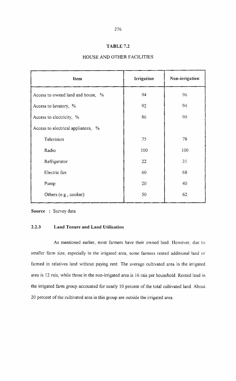
276

TABLE 7.2

HOUSE AND OTHER FACILITIES

Item Irrigation Non-irrigation

Access to owned land and house, % 94 96

Access to lavatory, % 92 94

Access to electricity, % 86 90

Access to electrical appliances, %

Television 75 78

Radio 100 100

Refrigerator 22 31

Electric fan 60 68

Pump 20 40

Others (e.g., cooker) 50 62

Source Survey data

2.2.3 Land Tenure and Land Utilization

As mentioned earlier, most farmers have their owned land. However, due to

smaller farm size, especially in the irrigated area, some farmers rented additional land or

farmed in relatives land without paying rent. The average cultivated area in the irrigated

area is 12 rais, while those in the non-irrigated area is 16 rais per household. Rented land in

the irrigated farm group accounted for nearly 10 percent of the total cultivated land. About

20 percent of the cultivated area in this group are outside the irrigated area.

277

Paddy is the most important crop in irrigated farm group sharing 51 percent of

the cultivated area in wet season, and rubber which shares 36 percent of the area. In nOI1-

irrigated farm group, on the contrary, area planted to rubber is 56 percent while only 25

percent are paddy land. It is surprising that only 51 percent of the farmers in irrigated area

reported using irrigation water. In dry season, very few farmers grew paddy.

2.2.4 Production and Distribution of Farm Products

In both irrigated and non-irrigated areas, paddy is grown mainly for sale. The

average product per grower in irrigated area was 2,100 kg, of which 750 kg was sold at the

average price of 4.5 baths per kg as shown in Table 7.3. It can be observed that paddy is a

cash crop in the study area. Therefore, there is incentive to grow it in the dry season

despite the government effort to promote high yielding rice variety as the second crop.

Moreover, there is more opportunity to work in rubber plantation. Hence, effective

utilization of irrigation water in dry season is accomplished.

2.2.5 Cost and Return per Hectare of Paddy

Table 7.4 illustrates cost and return per hectare of paddy cultivation in wet

season of both irrigated and non-irrigated areas. Cost of production is divided into cash

cost and non-cash cost, which includes cost of unpaid family labor and owned inputs.

There was no significant difference in the cost of production between irrigated and non­

irrigated areas. A slightly higher cost of production in the irrigated area was mainly due to

more fertilizer application and harvesting cost. Yield per ha, in the irrigated area was 1,250

kg, 250 kg higher than in the non-irrigated area. The average selling price was also higher

at 4.50 bahts per kg. Due to relatively low yield and high cost of production, the nOI1-

278

irrigation area show negative (-190 baht) net return. However it only cash cost is

considered, net return over cash cost was 4,850 bahts per ha, in the non-irrigated area, and

5,445 bahts per ha, in the irrigated area.

Cost and return of paddy in dry season is shown in Table 7.5. Due to unusual

low yield at 112 kg per ha, net return over cash cost was only 3,640 bahts per ha.

2.2.6 Family Income and Expenditure

Gross family income is shown in Table 7.6 Para-rubber is the major income of

farmers in both the areas. For those who do not grow rubber, working in rubber plantation

also provides reasonable income. The overall gross income per family was 50,300 bahts in

the irrigated area and 77,200 bahts in the non-irrigated area. This higher income in the non­

irrigated area is partly due to larger land holding. Annual household expenditure classified

by type of expenditure is illustrated in Table 7.7. Food was the major item expense in both

the areas, (37.5 percent of the total expenditure). It was followed by expenditure on

education of family members, (26.96 percent and 25.51 percent respectively) in the

irrigated and the non-irrigated areas.

2.2.7 Indebtedness of Farmers and Source of Credit

Indebtedness of farmers reveals the standard of living and the opportunity to

invest. It was found that 24 percent of the farmers in the irrigated area borrowed money

from different sources. The major source of credit was neighbour, sharing of 50 percent of

those who reported indebtedness in the irrigated area and 40 percent in the non-irrigated

area as is shown in Table 7.8. The average loan was 4,500 bahts and 12,200 bahts per

borrower in the irrigated and the non-irrigated are respectively. This loan, however, was

279

not totally for farming purpose. About 38 and 40 percent of the borrowers reported that

borrowing was for household consumption.

2.2.8 Flood Damages before and after the Construction of Dam

Percentage of farmers in the irrigated area who reported damages by floods

increased from 77 percent to 81 percent after the dam construction. This was, according to

the farmers, due to the blockages of flow during irrigation canal construction. However,

flooded area declined from 40 to 31 percent of the total area, and the damage cost

decreased from 482 to 344 bahts per household.

In the non-irrigated area, construction of the darn reduced the damage area

from 43 to 35.7 percent of the total area, and the damage cost decreased from 57l to 232

bahts per household. Therefore, it can be concluded that the construction of the dam has

positive effect in reducing flood problem.

280

TABLE 7.3

PRODUCTION AND DISTRIBUTiON OF FARM PRODUCTS

Area Total Distribution of product Ave. planted product

Home sale Crops per per Other

Sold Consumption Price grower Grower

kg bahtl kg ha Kg

Irrigation Area

Wet season 1996/97

Paddy 1.2 2,100 750 1,200 150 4.5

Rubber 1.1 1,440 1,440 - - 21

Dry season 1997

Paddy 0.8 900 550 300 50 4.5

N on-irrigation Area

Wet season 1996/97

Paddy 1.0 1,500 - 1,500 - 4.5

Rubber 5 4,000 4,000 - - 21

Source Royal Irrigation Department.

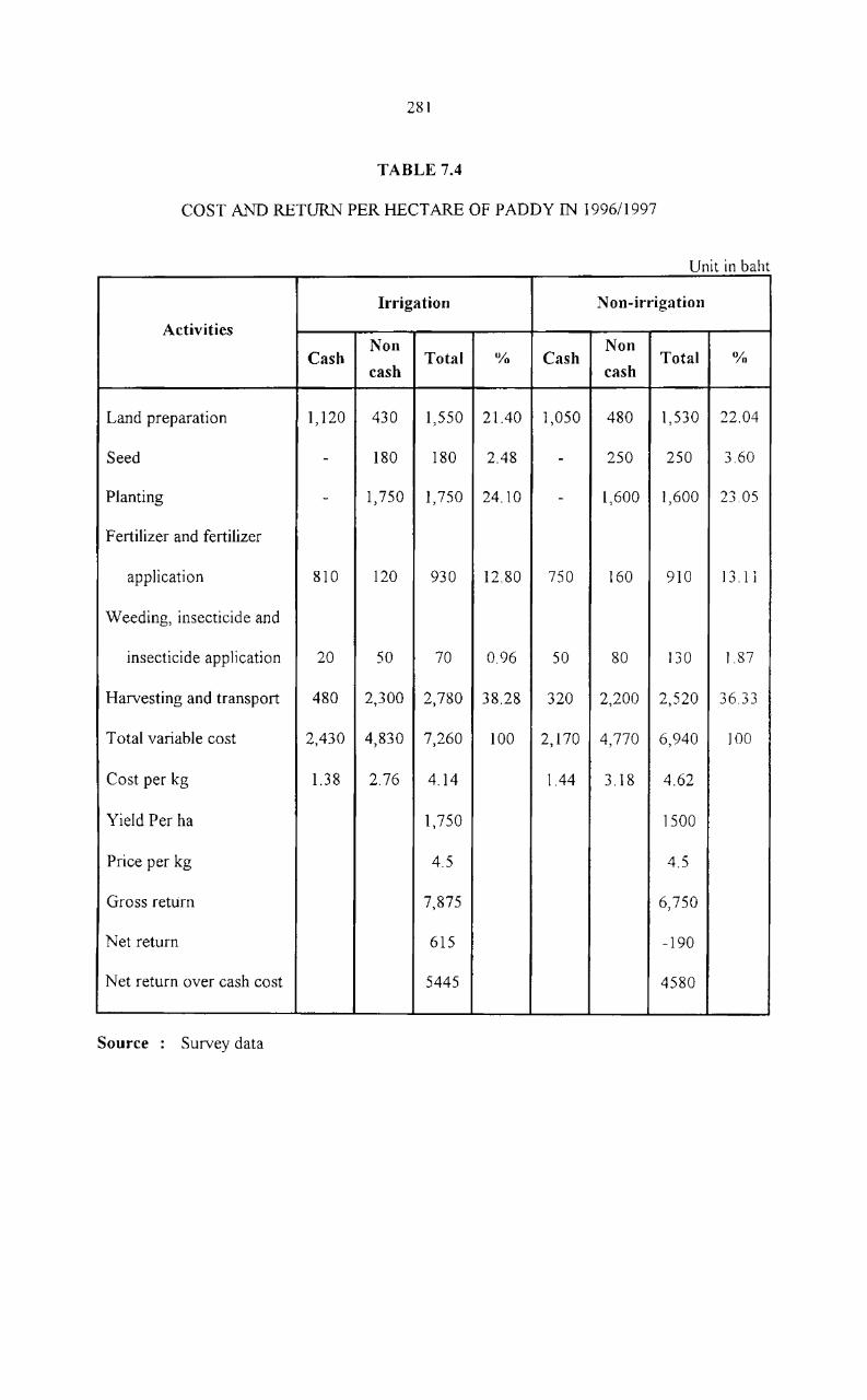
281

TABLE 7.4

COST AND RETURN PER HECTARE OF PADDY IN 199611997

Unit in baht

Irrigation Non-irrigation

Activities Non Non

Cash Total 11'0 Cash Total O/" cash cash

Land preparation 1,120 430 1,550 21.40 1,050 480 1,530 22.04

Seed - 180 180 2.48 - 250 250 3.60

Planting - 1,750 1,750 24.10 - 1,600 1,600 2305

Fertilizer and fertilizer

application 810 120 930 12.80 750 160 910 13.11

Weeding, insecticide and

insecticide application 20 50 70 0.96 50 80 130 1.87

Harvesting and transport 480 2,300 2,780 38.28 320 2,200 2,520 36.33

Total variable cost 2,430 4,830 7,260 100 2,170 4,770 6,940 ]00

Cost per kg 1.38 2.76 4.14 1.44 3.18 4.62

Yield Per ha 1,750 1500

Price per kg 4.5 4.5

Gross return 7,875 6,750

Net return 615 -190

Net return over cash cost 5445 4580

Source Survey data

282

TABLE 7.S

COST AND RETURN PER HECTARE OF PADDY IN IRRIGATED AREA

DURING 1997

Unit in baht

Activities Cash Non-cash Total fYt,

Land preparation 480 860 1340 22.64

Seed - 150 150 2.53

Planting - 1200 1200 20.27

Fertilizer and fertilizer application 780 30 810 13.68

Weeding, insecticide and insecticide

application ]60 60 220 372

Harvesting and transport - 2200 2200 37.16

T ota1 variable cost 1420 4500 5920 100

Cost per kg 1.26 4.0 5.26

Yield per ha 1125

Price per kg 4.5

Gross return 5062

Net return -858

Net return over cash cost 3642

Source: Survey data.

283

TABLE 7.6

FAMILY INCOME CLASSIFIED BY SOURCES OF INCOME

Irrigated N 00- Irrigated

Sources of income No. of Ave. income No. of Ave. income

Household Baht/year household Baht/year

Paddy 47 5,850 28 4,500

Para-rubber 34 30,240 32 84,000

Fruit tree 26 18,600 18 15,800

General merchant 3 72,000 4 75,000

Hired labour (rubber

tapping) 29 12,600 20 12,800

Hired labour (other farm

and non-farm work) 28 14,400 16 14,600

A verage income per

50 50,300 50 77,200 Household

Source Survey data.

284

TABLE 7.7

HOUSEHOLD EXPENDITURE IN IRRIGATED AND NON-IRRIGATED AREA

Irrigated Non-irrigated

Type of Expenditure

Bahtlyear 'Yo Baht/year %

Food 18,000 40.40 21,000 35.72

Clothing 2,000 4.40 2,500 4.85

Medical care 100 3.30 2,000 3.40

Travel expense 3,000 6.70 3,100 6.12

Recreation 1,200 2.60 1,500 2.55

Tuition 12,000 26.96 15,000 25.51

Electricity 1,800 40.00 2,000 3.40

Religious & donation 1,000 2.00 1,200 2.04

Others 5,000 11.20 10,000 17.00

Total 44,500 100 58,800 100

Source Survey data.

285

TABLE 7.8

INDEBTEDNESS OF FARMS AND SOURCES OF CREDIT

Item Irrigated Non-irrigated

Percentage of farmers with debt 24 12

Average loan per borrower, baht 4,500 1,200

Source of credit, %

Neighbour 35 30

Relative 50 42

BAAC 15 28

Objective of borrowing, %

Purchasing of land 12 8

Farming activities 40 50

Household consumption 38 42

Source Survey data.

2.3 Resettlement Area

2.3.1 Scope and Methodology

Field survey was conducted in the resettlements. Sample farms were randomly

selected from the two locations. Number of samples is approximately 25 percent of the total

households who actually resided in the area at the time of this survey, including 80 farmers

who were head of the families. There are no differences in general characteristics between

farm samples from different settlements. AB farmers in the resettlement area are Buddhists

286

2.3.2 Land Ownership and Animals

Before joining the resettlement programme, the farmers reported having an

average of 25 rais per household of Para-rubber plantation. At present, farmers in Ban

Pattana (Pattana village) are allocated 19 rais of Para-rubber per household. However, most

farmers also maintain Para-rubber plantation outside the resettlement area at an average of

10 rais per household.

3.3.3 Household Income and Expenditure

Para-rubber was the major source of household income 74 percent prior to

joining the resettlement program, this can be seen from Table 7.9. At present, share of

income from para-rubber declined because of immaturity of Para-rubber plantation.

However, income from fishery has increased drastically for farmers living in the

resettlement area. On the average, household income declined after moving into the

resettlement area. Table 7.10 illustrates annual expenditure of farmers in the two locations

by types of expenditure. Food was the major type of expenditure sharing more than 50

percent of the total expenditure.

287

TABLE 7.9

AVERAGE ANNUAL HOUSE INCOME BEFORE AND AFTER RESETTLED

Source of income Before resettled fY-, After resettled fY-)

Para-Rubber 24,800 74.35 36,400 67.14

Fishery 1,680 4.32 6,800 12.54

Para-rubber tapping 2,800 8.05 4,250 738

Hired 4,450 13.28 6,760 12.48

Average 33,730 100 54,210 100

Source Survey data.

TABLE 7.10

AVERAGE ANNUAL HOUSEHOLD EXPENDITURE IN 1996/1997

Expense Baht % of the total

Food 16,000 50.31

Clothing 1,800 5.66

Medical Care 1,600 5.03

Education 10,000 31.45

Recreation 1,000 3.14

Religious & donation 800 2.5\

Electricity 600 1.88

Average 31,800 100

Source Survey data.

288

2.3.4 Household Assets

Values of house and other properties, excluding land, were estimated in order

to value household assets as shown in Table 7.11.

2.3.5 Saving and Indebtedness

Apart from income and expenses, farmers were also asked whether they have

any saving. It was found that 58 percentage of farmers can save in such location. Farmers

in Ban Pattana prefer to save their money by keeping cash or gold at home. However,

about 30 percent of those who can save reported depositing money in the bank. More than

10 percent are keeping in the form of land and others.

The percentage of farmers with debt were quite similar in all locations at

around 30 percent of farm sample. Values of loan per borrower in Ban Pattana averaged

between 1,000 to 5,000 bahts. Nearly half of the borrowers used the money for household

consumption and neighbors were the most common source of credit. Some of the farmers

borrowed money from relatives, Bank of Agriculture and Agricultural Cooperative

(BAAC), and merchants.

2.3.6 Standard of Living before and after Resettlement

Farmers were asked to compare their ways of life in various aspects during the

periods before and after moving to the resettlement areas. There is no significant difference

in the responses to the questions. Maj ority of farmers reported better housing, better public

utility and security. A bout half of the farmers reported better standard of living, 8 percent

reported no change, and 2 percent worse, than before. However, on an average, around 5

289

percent of the farmers wanted to migrate from the resettlement area, especially farmers

having insufficient farm land and less opportunity to earn a living.

TABLE 7.11

HOUSEHOLD ASSETS AND ELECTRICAL APPLIANCES

Unit: In Baht/Household

Properties Values (Baht) ·Yo of The Total

House 96,000 61.85

Car 15,600 10.05

Motor cycle 24,000 15.46

Boat 6,000 3.87

Radio 4000 2.58

Television 4,500 2.89

Refrigeration 4,200 2.70

Sewing machine 450 0.29

Electric cooker 360 0.23

Electric fan 180 0.12

Average 155,210 100

Source Survey data.

290

2.4 Village Profile in the Phum Duang River Basin

The overall objective of this section is to describe the socio-economic structure

of household in the basin. Data and information used in the analysis were obtained from

the survey of the Community Development Department, covering 268 villages in the rural

areas of the basin. Results of the analysis are used as basic information for the

environmental development planning.

The Phum Duang river basin covers an area of about 4,668 km2 in Surat Thani.

The area can primarily be divided into upstream and downstream areas. Upstream area

refers to the area upstream of Rajjaprabha dam which includes the reservoir area and the

resettlement area. This upstream area accounts for nearly half of the basin. The

downstream area, however, varies in both physical and socio-economic conditions. The

Phase I irrigation project in Amphoe Phun Phin presently under construction is planned to

develop about 23,100 ha of paddy land. And another 50,000 ha has also been planned for

Phase II irrigation development. Therefore, to reflect these different basin geographical

features and specific urban characters of Muang district and Phun Phin district the village

profile has been segmented into 6 different zones (Figure 7.1) as follows.

Sub basin I

Sub basin II

Sub basin III

Sub basin IV

Sub basin V

Sub basin VI

Khlong Saeng Sub basin Area.

Khlong Sok Sub basin Area.

Downstream Area Outside Irrigation Area.

Khlong Yan Sub basin Area.

Irrigation Area.

Coastal and Urban Area

291

Socio-economic structure of each individual sub-basin IS described In the

following sections.

(1) Sub basin 1 : Upper Catchments Area

Sub basin 1 consists of 3,505 households in 29 villages, excluding the urban

area of Ban Ta Khun district. The total area covers about 1,435 km2, of which 78 percent is

forest area and 3.35 percent is rubber plantation. The population of this sub basin is 1,2318

persons with a population density of 6.1 persons per km2, and a growth rate of O. 05 percent

annually.

Since rubber area covers 3.35 percent of the total area, 90 percent of the

households are involved in rubber plantation as rubber is the main source of income,

averaging 36,000 bahts per household annually. Fisheries are also another source of

income for households living near the reservoir. Almost all villages in this zone receive

health volunteer services. However, nearly half of the villages showed high incident of

malaria.

(2) Sub basin n Khlong Sok Sub basin

Sub basin n covers villages in Pha Nom district. There are 5,405 households in

53 villages. The total area covers about 1,211 km 2 . The population in this sub basin is

27,330 with a population density of 22.5 persons per km2, and a growth rate of 0.57

percent per year.

Ninety percent of the households in this sub basin earn their income from

rubber, with an average of 21,000 bahts per household. Thirty-five percent of the

292

households also earn their incomes from fruit crops and field crops. It was reported that 86

percent of the households farmed in their own land. Health conditions of households in

Zone 2 are the poorest among the different zones. Almost all villages in this zone show

high incidence of malaria both in children and adults.

(3) Sub basin Ill: Downstream Area Outside Irrigation Area

Sub basin III covers the basin area located downstream from Rajjaprabha dam

and upstream from the Phase I and Il of irrigation projects. It covers Khirirattha Nikhom

district with a total area of about 314 km2. The total population is about 20, I 14 persons,

with a population density of 61.1 persons per km2. Population growth in this downstream

area is higher than the upstream areas, about 0.42 percent per year.

Even though paddy land shares only 7 percent of the total area, 29 percent of

the households grow rice mainly for their own consumption. Rubber is the important

source of income, contributing to about 70 percent of the households of this sub basin

while another 25 percent of the total households earn their incomes from fruit crops.

Eighty two percent of the farmers in this sub basin farmed in their own land, and 83

percent of the villages also reported having farmers associations. Health problem in this

downstream area is less serious than those in the upstream area since less than 15 percent

of the villages reported having incidence of malaria.

(4) Sub basin IV: KhIong Van Sub basin Area

Sub-basin IV covers about 1,178 km2 with a population of about 16,200

persons. There are 33 villages with the largest number of households (3,508). About 80

percent of this area are covered with forest, and 15 percent is rubber plantation. The

293

population density is at 13.7 persons per km2, with a population growth of 1.01 percent per

annum. Only small number of households receive income from other cash crops, such as

fruit trees. Standard of living of households in this sub basin is not much different from

those located outside the area.

(5) Sub basin V Irrigation Area

Sub-basin V is the proposed Phase I irrigation area in Phun Phin district and

Muang district of Surat Thani province. It covers about 350 km2 and 94 villages. Fifty tlve

percent of the area is rubber plantation and 38 percent paddy land. There are about 63,052

persons living in the area, with a population density of 1 19 persons per km2. Population

growth rate is the highest in all sub-basins (l.26 per annum). Since it is close to the urban

area, public utility and health service are better than the other areas. It was found that 96

percent of the villages have electricity and almost all the villages have health volunteers.

Rice is the major crop in the area. Eighty-two percent of the households engage

in paddy cultivation. Rice and rubber is the main cash crops of 67 percent of the total

households with an average income of about 68,000 bahts per year. Households in some

areas also earn additional income from fruit crops. Due to better public utility, this zone

has less health problem, especially concerning malaria.

(6) Sub basin VI: Coastal and Urban Area

Sub-basin VI covers a large portion of the coastal area. The total area of this

zone IS 298 km2 with a population of about 74,600 persons. Nearly 60 percent of the

population IS involved In paddy cultivation. Field crops and fruit crops are important

294

sources of income (72,400 bahts per household). In addition to farming, people living

along the coast also earn their living from fisheries and coastal aquaculture.

2.5 Conclusion

General characteristics of various parts of the project area as well as SOCIO­

economIc structure of households in the basin are considerably different. For the upper

catchment area where most of the area is covered with forest and rubber plantation, the

development should be considered the appropriate allocation of land between forest and

rubber plantation. In the reservoir and resettlement area where rubber and fisheries are two

important sources of income, the development should gear toward the improvement in

quality of life of the residents by providing better living conditions as well as occupation

opportunity.

Downstream areas consist of irrigation area, non-irrigation area, coastal area,

and urban areas. The irrigation areas, though yet to be completed, has good potential paddy

production, while outside the irrigation area rubber is the main source of income. In the

coastal area, on the contrary, aquaculture promotion should be emphasized. The urban

areas of Surat Thani are the concentration of commerce and industries with high

population density. They both are the major demand centers for water supply, and the main

sources of water pollution. The development of urban areas should take into account the

impact caused by water pollution in the coastal area, so that the environmental condition of

the coastal area can be maintained.

295

FIGURE 7.1

Ampl.oe ChOiio

•

" .AmpIloe r~Cbak

LEGEND:

Basin Boundary

Subbasin Boundary

Khlong and River

o ~ 10 15 20 "n> . .-. ---­~

GRAPHIC SCALE

SUP-BASIN IN THE PHUM DUANG RIVER BASIN

296

3. PUBLIC HEALTH AND NUTRITION

3.1 Introduction

These development projects are undertaken in order to improve the economic

situation of the country as a whole, and of the population in the project vicinity in

particular. Although the overall economIC situation may be favorably influenced by the

water resources development, the immediate effects on health and well being of population

groups in the neighbourhood of dams and reservoirs need to be assessed. Environmental

changes usually accompany the creation of artificial lakes, which may provide favourable

environment for the survival of great number of intermediate hosts, such as snails, and

mosquitoes that transmit diseases such as malaria, elephantiasis, schistosomiasis.

3.2 Objectives

The objectives of this study aspect include:

(a) To study the health and nutrition profiles including the parasitic infection,

sanitation and quality of drinking water of the people in the resettlement

areas.

(b) To assess the endemic vector-borne diseases and intermediate host created

from the reservoir; and

To fulfil these objectives various study aspects are carried out including health

and nutrition status, parasitic infection, malacology, malaria, and drinking water quality.

297

3.3 Methodology

collection.

This investigation has been carried out using the following methods of data

(a) Health and nutrition data were collected by questionnaire enumeration and

from interviews with responsible staff members related to health centres;

(b) The data about: (i) nutritional status of preschool children from birth up to

60 months old, (ii) Parasitic infections rates of intestinal helminthes and

trematode, (iii) malaria and (iv) logic of freshwater snails and clams, were

obtained from medical and health division of the EGA T 's reports.

Cc) Water samples from sources of water consumption of the majority or

villages were examined for their physical, chemical and bacteriological

properties according to the Standard Methods.

3.4 Study Area and Population

The resettlement villages are considered to be more influenced by the

Rajjaprabha dam. Residents in this village is referred to in this study as the "study group".

Another village called Ban Khao Sok is also located near the dam site in Pha Nom district,

but it is not influenced by the dam and reservoir, hence regarded as the "control area" in

this study.

3.5 Health and Nutritional Status of the Villagers

In assessing the health and nutritional status emphasis was made on the most

vulnerable groups in the community, which included pregnant and lactating women,

298

newborn infants and preschool children up to 60 months of age. Adverse effects on health

and nutrition are normally recognized in these groups first.

3.5.1 Mother and Child Health

The number of newborns in the 2 villages under investigation within the past

12 months had been assessed through questionnaires. From the total population 7 babies or

5.5 percent of population had been born in the last 12 month. The age of the mothers

ranged from 17 to 38 years. The number of boys born were in excess of girls with a ratio of

1.75 : 1.58.

At the time the questionnaires were completed, only 5 women were pregnant in

the 2 villages. Judging from this small number of current pregnancies, attendance of

prenatal care was poor because only 3 of the women made use of this service, either in the

hospital, health station, or mother and child health (MGH) center. The other two were

either afraid, or claimed that they did not like to use such services.

Only one infant death was reported in Khao Sok village, during the least 12

months. There was no death in other villages. The death in Khao Sok village was due to

acute and preventable infectious diseases such as diphtheria, tetanus and measles.

3.5.2 MCH Care in the Health Station

In order to get a better picture about family health, particularly of women and

their children, information was collected from those mothers who had children of 0 to 5

years. Information collected indicated that all deliveries which took place at the health

stations were without complications. This may be due to the fact that only those women

299

who did not expect any complication incident while giving birth delivered at the health

stations. According to the responses of the mothers, majority of birth attendants in the

health station were traditional midwives. There was only one qualified midwife in the

health station.

Weight at birth is an indicator of the nutritional status of women in the child

bearing age. Records were incomplete on this aspect particularly for the control village at

Ban Khao Sok. Information collected show that 50 percent of the parents adopted family

planning. The reasons for not adopting family planning were religious belief, and

uncertainty on safety. Some of the villagers simply did not want to practice it because they

wanted to have more children.

3.5.4 Nutrition

A semi-quantitative survey was undertaken in order to find out the dietary

pattern of the population. The staple food of all villages under investigation was rice. Milk

vegetable oil and lard were used to a great extent for cooking purpose. Generally green­

leaf vegetable was very popular in the whole study area, whereas fresh fruits were not

commonly consumed on a daily basis. Kinds of supplementary food include rice, banana,

egg, chicken, fish, milk and sweetened condensed milk. It appeared that supplementation

was inadequate as it was started too early. In the majority of investigated cases

supplementary feeding started at the age range between 1 to 4 months, when it should

actually start after 4 months. On the other hand, the children who were weaned too late

were observed during pregnancy by approximately 20 percent of the women questioned.

Between 50 percent to 90 percent of all women questioned observed some food taboos in

the lactating period. The reason for observing food taboos during pregnancy was the belief

300

that eating certain kind of food will result in omitting, mornmg sickness, and even

abortions. Reasons for avoiding certain food stuffs in the lactating period were fears such

that the wound healing would be impaired, the muscle might ache, the construction of the

uterus might not take place or this organ might be infected, the edema might occur or it

might cause stomach-ache. Sometimes special reasons could not be given, only a general

fear towards certain food staffs was expressed, or it was claimed that the midwife did

advice to restrict certain food items.

The nutritional status of preschool children judged from anthropometric

measurement seems to be quite good. Based on the Gomez classification (WHO. 1976),

and a Thai standard, abnormal nutritional status was found only in Khao Sok village where

11 percent of the preschool children were underweight of the second and third degree.

About 9 to 12 percent of the school children in the resettlement villages were found to be

malnourished. This is better than the condition in the control village of Khao Sok village in

which about 14 percent were malnourished. However it should be kept in mind that quite a

number of children are rather short, so the weight seems to be appropriate to their height.

When judging the overall nutritional status of all preschool children according

to the SD scores in comparison with the North American standard, (W. KelIer, WHO

Bulletin 1977) it appears that the weights of the children fairly relate to their heights in the

resettlement village.

3.5.5. Utilization of Health Stations

The overwhelming majority of the villagers used the service of health stations.

The most common reason for this was to purchase medicine when they had fever. In quite

301

a number of cases the visits to health stations were for the treatments of malaria and

gastrointestinal infection.

3.5.6 Morbidity

About 75 percent to 80 percent of the interviewed samples in the villages

claimed to have been sick during the previous 12 months period. Almost all cases were

infectious diseases. Malaria was quite prevalent in the area, ranging from 20 to 45 percent

of all cases reported by the two villages. About 30 to 40 percent of the villagers were sick

because of common cold. Approximately 20 percent of the cases, patients suffered from

ill-defined diseases claimed as fever.

3.6 Study on Parasitic Infection

Data were obtained from EGA T. The results shown indicate rather high

prevalence of parasitic infection in all investigated villages, with the highest prevalence in

the control village at Khao Sok village, the detail of protozoa and helminthic infections as

follows.

3.6.1 Protozoal Infection

The prevalence of Entamaeba ~, Entamaeba histolytica, Giardia lamblia in

the two investigated villages were about 6 to 12 and 2 to 7 percent in Khao Sok village and

Pattana village respectively. Entamaea roli, Entamaeba histolytica and Giardia lamblia

were the main protozoas prevalent in all villages, indicating contamination of food and

drinking water. These parasites cause dysentery and/or diarrhea.

302

3.6.2 Helminthic Infection

The prevalence of hookworm, Ascasis lumbricoides and Trichuris triciura in

the two investigated villages were about 20 to 43 percent and 5 to 36 percent is Khao Sok

village and Pattana village respectively. Helminthic parasites in the investigated area are

soil-transmitted helmiths (Hookworm, ·As. Lumbricoides, T. trichiura). Hookworms can

enter human body through larva penetration through the skin. Hookworm eggs are excreted

in feces, and under favourable conditions the eggs will develop into infective larvae within

one week. They can survive for many months in the soil. Men get infection from eating

food and vegetables contaminated by the eggs, and unhygienic personal habits.

The investigated villages are therefore endemic for soil-transmitted helminths

and protozoa due to poor environmental sanitation and lack of personal hygiene.

3.7 Malacological Study

There were reports of widespread snail intermediate host (Bithnia Snail), and

of Thai liver-fluke (Opisthorchiasis) after reservoirs were created, especially III the

northern and north-eastern part of the country due to bad habit eating raw fishes.

In the resettlement areas, many samples of clay and silt from the bottom of

reservoir and waterways were examined. But nowhere water snail was found. This result

was confirmed by parasitic survey in the resettlement areas and the control area of Khao

Sok village. Again no case of liver-fluke in the fecal samples was found.

303

3.8 Malaria Study

Evaluation of each year activity for the whole country at the end of 1995

revealed that malaria death rate was only 2.4 per 100,000 persons. Annual parasitic

incidence was 6.3 and the Slide Positive Rate (SPR) or percentage of positive cases as

examined from blood smears (Ministry of Public Health, 1995) was 4.6. But the malaria

situation in Surat Thani province from 1990 to 1995 was similar from that of the whole

country. It was found that in the beginning of 1995 the slide negative rate at Pattana village

was quite low, and dropped after May. The 6 month SPR value of Pattana village of about

8 percent was much lower than the value of about 9 percent experienced in Ban Ta Khun

district (during the same 6 months period in 1995). By this evidence, it could be said that

there was low malaria infection rate in Pattana village. At the time of peak infection rate

residual insecticidal spraying team was called from the Malarial Control Sector in Surat

Thani to spray in the houses around the villages. So the case dropped out in the following

months.

The SPR value of Pattana village was about 15 percent in 1995. However, the

monthly distribution of the SPR reveals higher rates only in August and September 1995.

At Khao Sok village, it was found that slide positive rate was about 18 percent in 1995.

The parasitemia had more or less the same pattern as Pattana village i.e. the parasite was

found in August, September and October. While slide positive rate at Khao Sok village

was about 5 percent only, the parasitemia was found in March, April and May, which had

the same pattern as Ban Pattana.

304

3.9 Drinking Water Quality

Six samples of drinking water were collected from the resettlement area: three

samples each from Pattana village, and Khao Sok village. It was found that all samples of

drinking water were rain water. The water supply provided by EGAT is runoff from the

mountain which is stored in a reservoir. It is distributed without any treatment. The quality

parameters of water such as hardness, chloride, and iron are within the standard of drinking

water. The physical quality parameters such as color and turbidity are very high, depending

on the seasons.

Most of the water samples contain high alkalinity, which is not suitable for

drinking. It causes irritation and itching. The residents of Khao Sok village (control area)

complained about itching when they take bath. Coliform bacteria is used as an indicator of

water contamination. The results show that most of the drinking water samples in these

two areas have higher bacteria content than the standard. It means that water is not safe for

drinking,. However the quality of the drinking water can be improved by filtration and

boiling.

3.10 Comparative Evaluation

An attempt is made to assess the change in public health status of the people

living in the study area. This is done by comparing the results of the pre-impoundment

study with those found in this study. Although the results are not, in a strict sense,

comparable due to differences in the methods of data collection and in the studied

population, they are compared for qualitative interpretation.

305

(a) Malaria situation in the study area has improved, although the values of

annual parasitic incidence (API) found are not much different. This is largely because of

the fact that many incidences were not reported in 1985 due to poor accessibility at that

time.

Parameters Pre-impoundment Post-impoundment Qualitative

Study Study Change

Malaria: Better

API 30,5/1000 (in 1985) 23.3/1000 (in 1995)

Parasite P.f. > P.v. P.f > P. v. Same

Intestinal parasitic 5.511000 90/1000 Not

comparable

Medical service usage 70.8% 97.6% Better

Mother and child health: Better

Completed vaccination 50.7% 60.8%

Family planning 14.9% 16.5%

Nutritional status : Same

Milk consumption 42.5% 20.3%

Green-leave vegetable

consumption 92.3% 91.9%

(b) Intestinal parasitic evidence is judged to be not comparable between the

two studies, although the stool examination in this study shows a much higher parasitic

infection rate. The very low rate of 5.511000 or 0.55% reported in the pre-impoundment

study seems unrealistically low for such a developing country as Thailand.

306

( c) Medical services and the mother and child health are better during this

post-impoundment period mainly due to the increased number of related facilities, and the

improvement in accessibility to the rural villages. Nutritional status was judged to be the

same during both periods, or slightly better after the impoundment.

307

4. TOURISM, RECREATION AND AESTHETICS

4.1 Introduction

The national tourism policy is to spread the benefits of tourism throughout the

country The development and promotion of Rajjaprabha dam and the surrounding area as

tourist destinations can play a part in spreading the benefits of tourism to the people of

Surat Thani province.

4.2 Objectives

The objectives of this study are firstly to reassess the tourist and recreational

potential of the dam after its construction, and to suggest how the dam might be promoted

as a tourism resource ; secondly to reassess the impact of dam on the aesthetic quality of

the environment; thirdly to reassess basic data on tourism so as to make a sound estimate

of the benefits from tourism in monetary terms.

4.3 Scope of Study

The study covered tourism resources (including aesthetics), tourist services and

marketing. Although the study area covers the Phum Duang river basin in Surat Thani

province, the study was concentrated on the Rajjaprabha dam. Tourism development was

studied to some extent at the regional and provincial levels but this was mainly to establish

the context for a more detailed study of the dam.

4.4 Methodology

The methods used in this study includes:

308

(a) Desk studies of secondary data;

(b) Questionnaire survey of visitors to the dam;

(c) Informal interviews with key personnel'

(d) Field study of tourism resources and services; and

(e) Travel cost approach to estimate the benefits of the dam In monetary

terms.

Further details of the methods used are presented in later sections of this report.

4.5 Regional Tourism Context

In assessmg; the regional context of tourism we can immediately identify a

triangle whose points are locations of relatively intense tourism activity, i.e., Krabi, Phang­

nga, Phuket, Surat Thani, Ko Samui, Nakhon Si Thammarat. These resorts attract

international visitors as well as visitors from Bangkok and other parts of Thailand.

Moreover all of them are still undergoing rapid development and are being vigorously

promoted by the Tourism Authority of Thailand (T AT). They have much more diverse and

attractive scenery than Rajjaprabha dam as well as a higher level of services and wider

range of available activities.

4.6 Provincial Tourism Context

4.6.1 Provincial Tourist Attractions

Tourist attractions in Surat Thani province which used to be the land of ancient

civilization some 1,200 years of age, with its center being situated around the area

nowadays known as Chaiya district. Many valuable and well known ar1s have been

309

preserved as the evidence of the old civilization. Besides, some religious assets of newer

historic periods and several attractions exist in this province. These interesting sites are

shown in Figure 7.2 a brif description of which is given below.

(1) Historical and Religious Assets

Phra Borommathad Chaiya : Phra Borommathad Chaiya is regarded as the

most important pagoda in the south. It is situated in the vicinity of Wat Phra Thad Chaiya

about I km from the district's railway station. The pagoda is of prime importance and

highly revered by Surat Thani people as well as the southern citizens. The pagoda is said to

contain a piece of the holy Bone of the Lord Buddha, and was built during the 11 Sri Vichai

period" which was more than 1,200 years old. The artistical construction patterns are

completely of the Sri Vichai Art which are relatively rare and valuable at the present time.

Wat Tham Singkhon : Wat Tham Singkhon is located in Khirirattha Nikhom

district approximately 35 km downstream from the proposed damsite. The temple was built

hundreds of years ago and, at present, serves as a center of religious reverence by local

people. A cave is also present in the vicinity of this monastery.

Wat Khao Phra Anon and Wat Nam Rob These two temples are the

ancient religious assets located in Phun Phin district. They are important monasteries and

are the centers of respects of the people of this district.

Wat Wieng Sra : This old monastery, which is about 100 years old, is located

in Wieng Sra district. In the vicinity of this district there exist some ancient remains and an

old town surrounded by a canal, dug to protect the town from enemies' attacks. These

remains are still present.

310

(2) Natural Attractions

Ko Samui Ko Samui is the largest island along the eastern shoreline of

southern Thailand and is the third largest island of the country. Actually, the term "Ko

Samui" represents groups of more than 80 small islands, located approximately 80 km off­

shore the town of Surat Thani. It possesses a number of attractions comprising several

waterfalls, beautiful beaches, other attractive scenaries and marine resorts. Ko Samui is

one of the well known tourist places in the southern region and of the country. Recently,

the highway department has been to construct a 80 Km long concrete pavement road

around the island to facilitate transportation on the island and to boost tourism potential of

the area.

Suan Mokkha Plaram : Suan Mokkha Plaram, locally called "Wat Tarn Narn

Lai ", is a religious institute located in a natural park of very beautiful, peaceful . and

pleasant surroundings. The park is highly suitable for Buddhists who want to study the

Buddhist Teaching. There is a religious study hall and an exhibition hall where religious

pictures are complied. Poems, and Lord Buddha's words are inscribed on the wall of the

exhibition hall.

Phum Rieng Village: Phum Rieng village is located in Chaiya district. It is

very famous in southern Thailand as a place, which produces hand woven silk cloths with

different patterns and styles. These products are also available on sale in the town of Surat

Thani under the trade mark "Pha Mai Phum Rieng"

Vana Uttayan Khao Tha Petch: Vana Uttayan Khao Tha Petch is a natural

park located along the highway linking Muang district and Ban Na San district

311

approximately 9 km from the provincial hall. The well-known Sri Surat Pagoda is present

at this place. There also exists a hill in this natural park, and the beautiful scenery of Surat

Thani town can be viewed from the hill top.

Ko Pha-Ngall Ko Pha-Ngan is another offshore island in Surat Thani

province where the district office is situated. It is located to the north of Ko Samui and is

surrounded by a number of small beautiful islands.

Beach in Don Sak District : This is a long and clean beach lying along the

coastline of Surat Thani province. A very long line of coconut is existing along the beach

with number of fishermen house scattered in line behind the coconut trees in the beach

presents an attractive scenery.

Uttayan Nok Nam : Uttayan Nok Nam, or water birds park, is located in the

vicinity of Khian Sa district. It consists of a pond where a great number of lotus plants are

grown, and is surrounded by an area covered with large trees and rolling hills, which

provide shade and peace to the area. There are thousands of water birds especially wild

ducks feeding and living in this area, thereby creating an interesting scenery in the park.

Water falls: There exist some beautiful waterfalls in Surat Thani province of

which the interesting sites are the following:

Na Muang and Hin Lad falls in Ko Samui district

Paeng and Tarn Sadej falls in Ko Pha-Ngan district

Viphavadee fall in Don Sak district

Eleven-Storeyed Waterfall: A beautiful waterfall has recently been

discovered by the National Park Division personnel of Royal Forest Department. It is

312

located in Khlong Sok village of Pha Nom district about 45 km from Ban Ta Khun district

along highway NoAO 1, and is said to consist of 11 steps of falls. The waterfall and

surrounding area had been in the process of proclamation as national park, and a plan has

been set up by the National Park Division to construct an office near the water fall.

4.6.2 Service Sector of Surat Thani

Tourist Accommodation facilities in Surat Thani : Accommodation facilities

are considered to be of prime importance which should be provided at a tourist place to

boost tourism potential of the place. According to the records obtained from the Surat

Thani provincial police station, such facilities, which are available in the province, at

present are described below.

(a) First class Hotels : Ta Pi hotel and Wang Tai hotel are the existing tourist

class hotel in the vicinity. It is located in Muang district and has total capacity of 618

rooms. Two hotels of the same class are under construction in the same district, and would

contain 480 rooms in total.

(b) Second Class Hotels: According to the most up-to-date record, there exist

18 hotels which can be regarded as the second class hotels with 968 rooms. Majority of

them are located in Muang district. Among these hotels, there are high quality hotels

comparable to that of the first class hotels with a total capacity of370 rooms.

In Ban Ta Khun district, where the proposed dam and reservoir will be located,

no hotels or tourist accommodation facilities of any kind exist at present.

313

GULF OF THAILAND

Locol;on No. Descripllon

Vana U~To)'on Knou 'To Per

2 WOI Nom ROb

:3 Wc, Khoo Phro Al'lonl

Suon Mokk~O Plo!.,pm

A(':'Ip~ O~ Cno, Ya 5

6

7

e U11oyon No\( Nom

9 W01 WQin~ Se

10 VipP'!,Jvcdeta Fclh

l\m,~':~e KG Sa:T'IUI

I~ Ko r~'\

~--~-- --------------~

1----------------1-1 r_.,-t~c-~-C-\.1 Cl J S C_C_C_" _____ -l

1--; _G--4-_'f_llUr n S 00 e: , '1. ~II":' ___ ---i

FIGURE 7.2

\

-(>--- Notional HU;J~woys

+-+---t-;, Roi I r 0 0 C

,0 Touri., Si' ••

~ hlf:'servolr 8ouncory

• Amohoe ( Dis1ricl)

@ ChcnQwOI ( Province)

ln1 erno 110nol Bound ory

Cl"lonqwo1 Soundor y

L o~u. Mop cl I 1,000,000 {,Ol'ft OfPottlfltnf 0' HiO"'w~~' 0,," 1)1 197!).

2. Tc\./,illn Aul~QI", e~ TP'lqilOlqL

LOCATION OF TOURIST SITES IN SURA T THANI PROVINCE

314

4.6.3 Tourist Activities in Surat Thalli

With respect to the tourist places mentioned in Sections 4.6.2 (1) and (2), the

most important one is Ko Samui, which is visited both by national and foreign tourists.

Another important site is Phra Borommathad Chaiya, which is toured mainly by domestic

tourists and by small numbers of international tourists. No official records of tourist at

these two sites are available, either at the TAT head office or at local government agencies:

With aspect to other tourist places in Surat Thani, visits by national and local

tourists are the main tourism patterns. At present there is a plan to develop it as a major

international tourist resort No mention of these places are there in the tourist records ..

According to data obtained form the Statistics Division of the TAT, hotel

occupancy record are available only for 1997. The records show that the total number of

visitors to Muang district in that year was 160,000 and that the monthly distribution was

relatively uniform. Due to lack of a long record of data, future trends of tourist volumes to

Surat Thani cannot be projected. According to the hotel records, majority of the visitors

were businessmen, with small numbers of government officials and tourists whose actual

destinations were Ko Samui and/or Chaiya district.

Southern Thailand is linked with the upper part by highway NoA from

Chumphorn downwards. This highway runs along the west coast, bypassing Surat Thani.

There is a highway along the east coast, passing through Surat Thani, Nakhorn Si

Thammarat and SongkhlalHat Yai. Thus, both of them are equally important as far as

tourism is concerned.

315

Surat Thani is linked with Phang-nga and Phuket by highway No. 40 1, but

domestic and local tourists who want to travel from Surat Thani to these two \vestern

provinces seldom use this route because of security problems. Rather they make a trip to

Songkhla first and then cut across to the western province via highway No. 4, normally by

regular local buses.

4.7 Natural Attractions and Aesthetic Quality in Proj ect Area

Existing natural setting along Khlong Saeng upstream of the damsite is quite

beautiful. In the vicinity of the proposed project, there are a number of beautiful natural

sceneries. A series of limestone and shale mountains exist along both banks of the stream,

and most of them are covered with relatively dense evergreen forests. The mountains are of

steep slopes, and precipitous cliffs are also present here and there, some of which extend

upward from the stream banks. Forests on slope complexes and on tops of high mountains

are still relatively virgin, due to difficult accessibility which makes forest clearing difficult

at most of these places. The mountains and forests combine to form pleasant sceneries of

the reservoir area, as shown.

On the left bank of Khlong Saeng, there exists the Khlong Saeng wildlife

sanctuary which consists of rich tropical rain forests. The areas above the high water level

of the reservoir also have pleasant natural aesthetic quality like the proposed reservoir. On

the right bank, which is composed of logging concessions at present, the area will be

converted to a forest reserve which would consist of a natural park. The remaining parts of

the prospective forest reserve will lie along the western shoreline of the reservoir area, and

the prospective natural park will be located near the reservoir shoreline. Parts of these

areas have aesthetic values, similar to that of the reservoir areas.

316

Khlong Saeng itself possess enough natural beauty. It consists of several turns

which presents interesting and pleasant views to new corners. Rapids consisting of large

rock outcrops exist in the stream at some locations. Large trees are present along the banks

in most areas except where villages and fruit tree plantations are located. Some of these

trees bear flowers at different seasons of the year, and some are naturally decorated with

climbers covered with numerous colorful flowers. In few areas, mountains and/or cliffs

exist on both banks forming a U shape with the stream. Since the proposed reservoir area

is difficult to access by land and since it is not an existing tourist place at present, the

natural beauty of the stream and surrounding areas seem to be of minor aesthetic value.

4.7.1 Market Analysis of Rajjaprabha Dam

The data recorded by EGAT officers for the years 1987-1996 show that the

number of visitors to the dam fluctuated from year to year (Table 7.12). January and

February appear to be the most popular periods to visit because of important long holidays

falling in these months. The number of visitors in other months is fairly uniform, and

seems to indicate that the amount of rainfall does not play a large part in determining

individual difference. However, it is still possible that the amount of rainfall has an effect

on the total number of visitors to the dam. Majority of visitors are Thais and a small

minority, foreigners. If we compare the number of visitors at Rajjaprabha dam and the

estimated number of visitors who stayed overnight at Surat Thani (there is an approximate

ratio is 1:5) we can conclude that Rajjaprabha dam has a better potential to increase the

number of visitors by increasing its share of visitors to the province. It should be noted

however that this figure does not represent the real number of visitors to the province as it

does not include day-trip visitors and visitors who stay with friends or relatives, or any

other non-commercial accommodation. If we use the real number of visitors the proportion

received by Rajjaprabha dam would be much smaller.

Unfortunately the EGA T officials only recorded the number of visitors and

therefore little is known about their characteristics, e.g., the province they came from,

income, etc. Such information would have been very valuable, and should be collected in

future.

TABLE 7.12

NUMBER OF VISITOR AT RAJJAPRABHA DAM

Year Number (Person)

1987 20,519

1988 61,662

1989 61,466

1990 64,207

1991 58,419

1992 58,546

1993 67,456

1994 71,172

1995 78,070

1996 88,048

1997 (Jan-Oct) 78,187

Total 670,986

Source From EGA T.

318

4.7.2 Visitors Profile and Experience from the Questionnaire Survey

This section presents the results of the questionnaire survey. The questionnaire

survey was conducted during two periods: i.e. from i h April to 12nd

April 1997 and from

5th to 10th January 1998. Questionnaires were distributed to approximately 25 percent of

the total number of visitors on each day of the survey. It was impossible to conduct random

sampling and therefore the sample was chosen "accidentaIly". This of course means that

the sample of visitors surveyed is not truly representative, and therefore the interpretation

of the results must be treated with caution. But it is earnestly that the data collected will

give acceptable indications for planning purposes. A total of 240 questionnaires were

collected, and tabulated. As was suspected, majority of the visitors to the dam came from

the southern provinces for the purpose of recreation. Male visitors slightly outnumbered

females. Most of the visitors were in the age range of 15-45. Majority of the visitors were

government officials or students. Majority (38.4 percent) of the visitors had an income of

3,001-5,000 bahts, 19.6 percent had an income within the range of 5,001-10,000 bahts and

more than 20 percent stated that they had no income. These were generaIly students who

were still supported by their parents. Majority of this latter group were generally well

dressed and brought with them enough food. So we can tentatively assume that most of the

visitors have enough income to spend on their trip if given the opportunity to do so.

Most of the visitors heard about the dam from friends or relatives, and this

support the idea that the best form of publicity is a good visitor experience. Very few

visitors came alone or with their family. Many chose to come with friends or colleagues.

Most of them came by private cars or rented buses. This may partly be a reflection of lack

of public transport in the area. Approximately 96 percent of the visitors came on a day trip,

319

but as accommodation is only available for official visitors one cannot conclude that

people do not want to stay overnight.

The preferred activity was enjoying the natural scenery. Viewing the type of

construction they had not seen before follows this.

Just over thirty percent revealed that they had been to Rajjaprabha on a

previous occasion, and this perhaps indicates their satisfaction with the experience. Tt also

perhaps indicates that if sufficient activities and facilities are provided it may not be too

difficult to persuade visitors to return. When visitors were asked to state what types of

facilities or services they would like to have at the dam the majority Gust over 32 percent)

expressed the view that they would like to have water sports and tour services. About 20

percent said that they would like to have food and souvenirs at the site while 10 percent

said that they would like to have accommodation. About 13 per percent wanted more

information or a guide service, and around 12 percent wanted improvement of the site.

Around 60 percent of the visitors to Rajjaprabha came as part of a day trip

itinerary. Among the most popular other places visited in Surat Thani were Ko Samui, Phra

Borommathad Chaiya, Khao Sok national park etc. The remaining 40 percent stated that

they intended to visit Rajjaprabha only. It seems likely, therefore, that these visitors

especially would be quite willing to stay longer at the dam site if more opportunities to

participate in some activities were available.

320

3.5 Summary of the Main Results

(a) There are high attraction of places in the Southern Region and the location

of Surat Thani town for tourism development. There is still plenty of opportunities to

attract a higher number of visitor from the lower southern part of the country.

(b) The quality and quantity of accommodation in Surat Thani is the obstacle to

tourism development. In fact as stated earlier even if the present number of tourists in Surat

Thani is doubled the average hotel occupancy rate would still only be around 85 percent.

(c) Rajjaprabha dam has a high potential to attract visitors from the lower

southern provinces and perhaps to a minor extent from Malaysia.

(d) Many visitors to Rajjaprabha tend to stop over only for a short time as they

also visit other nearby attractions. This suggests that one of the main strategies for

promoting Rajjaprabha is to promote it not only as a single destination but as part of a

route trip itinerary.

( e) Many visitors came to Rajjaprabha after hearing about it from friends. This

points to the importance of providing a good experience for visitors and thus encouraging

them to give Rajjaprabha some "free" advertising.

(t) Many visitors would appreciate the opportunity to participate in some kind

of recreational activity at the dam.

(g) Lack of regular public transport to the dam from Surat Thani as well as

around the surrounding attractions is an obstacle to tourism development that needs to be

tackled.

321

(h) Official promotion and marketing of Rajjaprabha and the surrounding area

may contribute significantly to counteracting the negative image of security in the

provlllce.

4.9 Present Benefit from Tourism in Monetary Terms

The travel cost approach is a way to put a monetary value on non-priced goods.

This approach was initially developed to value benefits received by consumers from their

use of an environment good such as a lake or a dam. The approach includes the price­

quantity reactions of consumers by examination of their travel costs. The main idea behind

this method is that the cost of travelling to a particular site influences the number of visits

made to it.

This relationship can be expressed as,

where

v

V

Te

=

number of visits,

travel cost,

other explanatory variables.

(7.1)

Observations on people using the dam site allowed the derivation of equation

7.1. This equation gives a prediction model explanation of visitation behaviour in terms of

travel cost and income.

For the second part of this approach, assumption is made that visitors to the

dam would react to the charging of an admission fee in the same manner as they would to

increase in travel cost to the site. If we accept this assumption then this allows the

322

visitation prediction model to be used to estimate visitation to the dam at various admission

charges by adding admission fees to the travel cost variable.

Although in reality no fees are charged, the assumption that changes in

admission fees affect the consumers the same way as changes in travel costs allow us to

predict visitation behaviour under various fee levels by using equation 7,1, and calculate

how consumers would react to similar increases in travel costs. The resulting price (fee)

quantity (visitation) observations provide a demand schedule for the site and can be

displayed in the form of a curve. The area under the curve gives a measure of the

consumer's surplus enjoyed by the visitors to the dam at zero admission fee (i,e" total

consumers willingness to pay) which is a measure of the value of the dam to its users,

An alternative method of estimating the benefits of the dam is to assume an

admission fee and multiply this by the predicted number of visitors. This was done using

the average willingness to pay from the questionnaire survey. Both methods of estimating

benefits are presented.

It must never be forgotten that the travel cost approach is based on a number of

assumptions and has a number of inherent shortcomings (M.M.Hufschidt, 1983)

Nevertheless used with caution it IS a convenient way of estimating the benefits of

resources development projects like Rajjaprabha dam when limited time and data are

a vailable. The details of the travel cost method as applied to Rajjaprabha dam are

presented below.

a r

323

•

[J

1

• Il .'\.1.1.\1' RAlHl,\ () ,\ M

FIGURE 7.3

" . .;

: Q ......

'"

, ... e· ."

ZONES USES IN TRAVEL COST APPROACH

0: .... -. ... ~ ... "

324

4.9.1 Application of the method to a valuation of the Benefits

(1) Introduction

To apply the travel cost approach we identified the recreation site (Rajjaprabha

dam) and divided the surrounding area into zones of increasing distance (taken as the road

distance between the main province center, Muang district, and the dam) which represent

increasing levels of travel costs. These zones are present in Figure 7.3 and Table 7.13. A

survey of users is then conducted at the recreation site to determine their place of visitation

rates, travel costs and some socio-economic characteristics. The standard charge of the

ordinary bus by the Department of Land Transport was used in place of the actual travel

costs as it was found that the results from the questionnaire were not clear. The information

from the sample of visitors is then analyzed and the data from this are used to measure

visitation rates on travel cost and income.

where =

TC

=

(7.2)

is the visitation rate (number of visitors from zone

per 1,000 population in zone),

is travel cost, and

IS mcome.

By the use of multiple regression, the hypothesis that TC do in fact have an

impact on visitation rates, was tested. The inclusion of income helped to eliminate the

effects of at least one component not related to TC out of total visitation rates (Eg. 7.2)

With the data present in Table 7.13 multiple regression was used to analyse the relation of

3 variables, viz., visitation rate, travel cost, and visitors income per year from each zone.

325

TABLE 7.13

BASIC DATA FOR TOURISM BENEFIT ESTIMATION

BY THE TRAVEL COST APPROACH

A. ZONE DATA*

Zone Distance Average Province

Total

km km Population

1 1-150 75 Surat Thani, Phang-Nga 1,574,680

Chumporm

2 151-300 225 Nakhon Si Thammarat 7,811,064

Ranong, Krabi and Phuket

" 301-450 375 Phatthalung Trang 1,554,685 .)

4 451-600 475 Songkhla and Satun 1,273,076

Pattani, Yala, 5 601-750 675 2,674,307

Narathiwat

* A number of visitor zones have been excluded from the calculations and from this

table as the number of visitors from these zones was so small. However an adjustment

has been made for this in the final calculation.

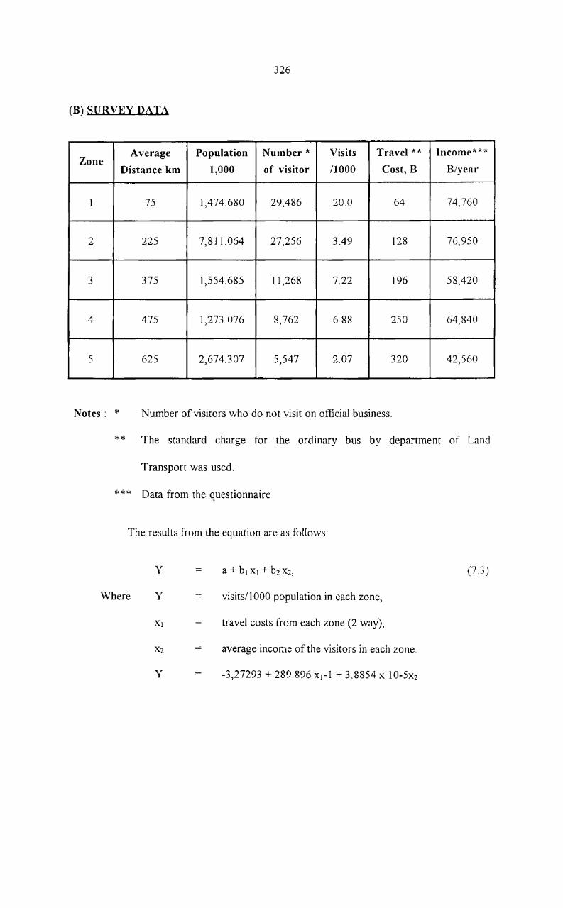
326

(B) SURVEY DATA

Average Population Number * Visits Travel ** Income*** Zone

Distance km 1,000 of visitor 11000 Cost, B B/year

I 75 1,474.680 29,486 20.0 64 74,760

2 225 7,811.064 27,256 3.49 128 76,950

3 375 1,554.685 11,268 7.22 196 58,420

4 475 1,273.076 8,762 6.88 250 64,840

5 625 2,674.307 5,547 2.07 320 42,560

Notes: * Number of visitors who do not visit on official business.

** The standard charge for the ordinary bus by department of Land

Transport was used.

*** Data from the questionnaire

The results from the equation are as follows:

y a + b l XI + b2 X2, (7.3)

Where Y "" visitsl1 000 population in each zone,

XI travel costs from each zone (2 way),

X2 average income of the visitors in each zone.

y -3,27293 + 289.896 xI-l + 3.8854 x 1O-5x2

327

From the results we can indicate that if Xl or travel cost increases the visitation

rate will decrease, and the visitation rate will increase with an increase in income, but the

rate of increase is very small.

(2) Demand Forecasting

From equation (7.3) the predicted total number of visitors In each zone IS

transformed by using the following formula.

7 -I -5

TV ~ Pi (-3.27293+289.896x X + 3.5734 X 10 X X')) ~J (7.4)

i~ 1 1 i

where TV Total number of visitor from all.

Pi = Population in each zone.

Xli Travel Cost in each zone.

X2i Average income of the visitors in each zone.

According to EGA T's records the actual number of visitors to Rajjaprabha dam

In 1996 for all purposes was 88,048. From the questionnaire survey approximately 62

percent of the visitors from the 5 zones identified came for recreation and 38 percent came

for official business. Assuming that these proportions are constant in future years the

predicted total number of visitors can be divided by the same proportions. An adjustment

can also be made for visitors from zones other than the 5 zones previously assumed to be 2

percent per annum until 2000, and then 1.1 percent per annum from 2000-2030. The

income growth of visitors in each zone is assumed to be 3 percent per annum from 1987-

2030. The total number of visitors is then forecaste as shown in Table 7.14.

PRIC

E 0

BAH

T No

. Of

14,2

0~

VIS

ITO

RS

---

180

170

160

I~O

140

~

130

~. 1

20

t::: 11

0 11

. a:

100

0 w

90

u

eo

a:

0-

70

60

50

40

30

20

10 °

0

to

~

50

7

0

90

10,7

13

7,0

80

4

,94

8

3,4

97

2

,42

9

--

--

--

5,0

00

1

0,0

00

NU

...e£

R

OF

VIS

ITO

RS

FIG

UR

E 7

.4

RE

CR

EA

TIO

N D

EM

AN

D C

UR

VE

IIQ

13

0 15

0

1,60

1 9

38

39

2

I~.OOO

167 -

I

V-J

N

0

0

329

TABLE 7.14

ESTIMATE OF AVERAGE ANNUAL TOTAL NUMBER OF VISITORS

Assumed Assumed

Year Total No. of Recreation OTHER population income visitors group Group growth rate growth rate

1995 78,070 14,196

1996 88,048 73,509 14,539 2 3

2000 91,652 76,445 15,207 1.1 * " .)

2005 98,468 82559 15,909 1.1 ., .)

2010 102,420 85,776 16,644 1.1 " .)

2015 114,870 97,455 17,415 1.1 " .)

2020 128,500 110,276 18,224 1.1 3

2025 146,480 120,085 26,395 1.1 " .)

2030 152,460 117,920 34,540 1.1 " .)

Note Growth rate according to the target set by the Eight National Economic and

Social Development Plan.

(3) Benefit from the Dam Received by Recreation Type Visitors

The estimated relationship can be used to determine how the visitation rate

would change if visitors were asked to pay for the experience of visiting Rajjaprabha dam.

The analysis assumes that visitors would respond to a fee the same way they respond to

travel costs. The analysis indicates how many visitors would be willing to pay for

Rajjaprabha dam's recreation environment.

330

The number of visitors in 1996 as shown III Table 7.14 IS used and the

Equation determines points on the demand curve.

From Figure 7.4 visitors who come for recreation would be willing to pay up to

the area under the demand curve. The area under the demand curve estimated in this

analysis is approximately 5,246,660 bahts. However if visitors come from some distance,

there may be other recreation sites.

Of assess that a trip to Rajjaprabha dam is not for a single purpose, then the

travel costs should be divided between the different sites. In fact according to the

questionnaire survey only 40 percent of the visitors visited the dam as a single destination.

The remaining 60 percent visited a total of 3 or 4 places including the dam. Therefore if we

divide the travel costs between the different sites then the results will be as follows:

(a) Benefit received by visitors who visited the dam only equal 5,246,660 x 0.4

= 2,098,664 bahts

(b) Benefit received by visitors who visited other places assuming Rajjaprabha

is allocated 30 percent of the total equals 5,246,660 x 0.6 x 0.3 = 174,240

bahts;

(c) The total benefit therefore equals 2,098,664 + 174,240 = 2,272,904 bahts or

25.8 bahts per visitor

331

However this result is only for those visitors who came for the purpose of

recreation.

(4) Benefit from the Dam Received by Non-recreation Type Visitors

For other visitors group, i.e., who come on official business, we can evaluate

the benefit by asking directly about their willingness to pay. The result from this method is

approximately 241,080 bahts or 14.7 bahts per visit. However this may well be an

underestimation, as, rather than use the bidding game technique the study simply asked

visitors how much they would be willing to pay. The bidding game technique, might have

elicited a higher sum.

(5) Benefit from the Dam by Expenditure of Visitors

The average total expenditure of visitors who visited the dam using data from

the questionnaire surveys works out to 147.5 bahts. The total benefit from visitors, based

on the actual number of visitors in 1996 is approximately 12,987,080 bahts. The same

principle of dividing travel costs between the various sites visited is adopted here. The total

benefit from the visitors at Rajjaprabha dam in 1996 is approximately 3,698,540 bahts.

By summing up these benefits we can see that the total benefit from market and

non-market sources is about 9,245,040 bahts, or 105 bahts/visitor in 1996. The benefits

have also been calculated up to the year 2029 and are presented in the section on the

evaluation of actual positive benefits.

332

5. ARCHAEOLOGICAL AND HISTORICAL VALUES

5.1 Introduction

In the pre-impoundment environmental and ecological study it was reported

that places of cultural values are present in the reservoir area. In this post evaluation

study, the archaeological and historical values are assessed for a much larger area, i.e ..

covering the whole Phum Duang river basin. This study identified altogether 5 sites of

archaeological and historical values by field survey and field interview techniques. These

sites include ancient settlement site; old palace, Buddhist monastery, and Royal Pavilion.

These sites are assessed on their significance, existing condition, and development

potential. Their original archaeological depositions have been severely destroyed by both

natural and human causes.

From this investigation, the archaeological sites of historical times were found

at the vicinity of project area. It can be concluded from the data that the Phum Duang river

basin used to be inhabited by historic men who might have later migrated to the plains of

Phum Duang river. In that period, men have moved into this area for tin mining. However,

there has been no evidence of continuation of habitation until about 150 years ago, when a

few families moved in this area once again, followed by many more and have stayed there

until recently.

5.2 Historical Sites

Archaeological sites in the historic period are rarely found around Phum Duang

basin and are not important as those belonging to the prehistoric period. Besides the

333

artifacts found historical values are mostly small in site. The archaeological sites of the

historic as well as the artifacts found during the survey are described below:

(1) Nai Mui village:

Ban Nai Mui village, there exists an abandoned monastery, which is about 150

years. The age of this monastery was estimated based on the information obtained from

the local villages and on the age of the Buddha images, which used to be kept here, but

have been removed to the new monastery at Bang Kaew village. Most of these images,

with lap size ranging from 5 to 7 inches were highly decorated in the artistic styles of

Ratanakosin during the reigns of King Rama Ill-IV. This monastery has been abandoned

for more than 30 years as described previously. The reason for this move was said to be

because of inconvenient communication with other villages, since the "Wat" was situated

deep into Khlong Mui, which is a small canal. The built-up structure of the "Wat" is made

of wood, which has mostly deteriorated, hence no permanent structure is left todays

(2) Pak Pae village:

There is a stone plate on which the royal signature of their Majestic the King

and Queen were inscribed to commemorate their visit to this village in 1969. Today, the

stone is placed in front of the flag staff at Ban Pak Pae School.

(3) Chiew Tae village:

In this village, here is an old silver coin. It is the coin of British currency,

valued one rupee, with English inscription: "Victoria Queen" on one side and "East India

Company one Rupee 1840" on the other side. This type of coin which is made of real

334

silver, might have been used in trading of tin ore in this area, probably in the reign of King

Rama V. Beside the said coins, other English, French, Spanish and Mexican silver coins

were found to have been in antique collections of villagers who used to live along Khlong

Saeng some of which to have been inherited from their ancestors. The age of these coins

vary, the newest being an English coin made during the reign of King Edward VlII in

1906. Although many coins were reported to be found around Ban Chiew Tae, no other

evidence of permanent settlement off historic were observed here.

(3) Chiew Tae village:

In this village, here is an old silver coin of the British with a value of rupee,

with English inscription: "Victoria Queen" on one side and "East India Company one

Rupee 1840" on the other side. This type of coin which is made of real silver, might have

been used in trading of tin ore in this area, probably during the reign of King Rama V.

Beside the said coins, other English, French, Spanish and Mexican silver coins were also

found to have been in antique collections of villagers who used to live along Khlong Saeng

some of which have been inherited from their ancestors. The age of these coins vary, the

newest being an English coin made during the reign of King Edward VIII in 1906.

Although many coins were reported to be found around Chiew Tae village, no other

evidence of permanent settlement of historic were observed here.

(4) Pak Ka village:

Traces of a historic settlement was found at the average elevation of 60 m

MSL, at Pak Ka village. These included British silver coin, which were found just like the

one found at Chiew Tae village. A Chinese coin was also found here. All these items

335

belong to the local people who said that they inherited them from the ancestors. This place

might use to be a village where people traded tin ore about 100 years ago. In addition to

these two coins, pieces of earthen-wares of historic times were also found around the

mounds near the village.

(5) Wang Khon village:

Evidences of historic human settlement was found at this village at elevation of

about 80m MSL at Wang Khon village, which included pieces of potsherds and Thai

copper coins of the reign of King Rama V. These items show that this area used to be

inhabited till around 100 years ago. The inscription on the front face of the coin (in Thai) is

"Chulalongkom" with the image of Phra Siam Dhevathirat and "one Solot" (in Thai) on

the rear face.

(6) Plai Saeng village:

This site used to be a community, dwelling area which was deserted some 50

years ago. An old abandoned wat was found together with remains of an old village near

the confluence of Khlong KhW1 and Khlong Saeng. Pieces of earthen-wares found here,

show traces of historic human dwelling at this site. It is believed that this area used to be a

large community since tin ores were reported to be present in large amount there.

The idea of using these archaeological sites in tourism promotion may need

further planning and evaluation. Because their development may not be economically

feasible. It may probably be more appropriate that the archaeological sites development be

aimed at the conservation of cultural heritage. And the utilization of the sites for tourism

promotion should be considered as the secondary objective.

336

Further archaeological and historical sites investigation and development

should involve a more detailed study taking into consideration the historical meaning and

significance of each site. Then only its real value and main attraction can be identifiecl.

Then systematic archaeological study, if found appropriate, should be carried out. Further

site development attempt should be made to maintain the original condition of the sites in

order to preserve their heritage values.

5.3 Conclusion

Investigation related the existence of SOIl1e archaeological sites of historical

importance at the vicinity of the project area. From this can be concluded that the Phum

Duang basin used to be inhabited by historic men. They might have migrated to the plains

of Phum Duang river. In that period men had moved into this area for tin mining.

However, there has been no evidence of continuation off habitation until about 150 years

ago, when a few families moved in this area once again, followed by many more and have

stayed there until recently.

The archeological impact is not economically quantifiable for two main reasons.

First, there are unknown sites suspected to be located under the reservoir. Since it is still

unknown whether it is possible to make any economic evaluation. Second, for the number of

known sites sunk under the reservoir there is no record of tourist visit upon which the

tourists' willingness to pay might be estimated. Therefore, we do not have any database to

assess the economic value of the archeological impact of Rajjaprabha dam at all.

CHAPTER VIII

ECONOMICS EVALUATION OF

ENVIRONMENTAL CONSEQUENCES

CHAPTER VIII

ECONOMICS EV ALUA TION OF ENVIRONMENTAL

CONSEQUENCES

The evaluation of environmental economics consists of three aspects: (i) the

implication or regional economics which is the evaluation at the regional level (ii) the

evaluation of actual positive benefits which is done at the project level and (ii) input-output

analysis which indicates the effects of the project implementation on the regional economy

of Surat Thani province.

1. Implication on Regional Economics

1.1 General Background

The macroeconomic impact of a project is evaluated to determine whether the

project is consistent with overall national, regional, and sectional objectives, and whether

the investment represents the best means of achieving the intended objectives. Hence, the

framework adopted for economic analysis of the project should depend on policy

objectives which include provision of basic needs of the people, provision of opportunities

for gainful employment, achievement of rapid and sustained economic growth, and more

equitable distribution of income among the various sections of the population. In other

words, the purpose of macroeconomic analysis is to determine the importance and urgency

of the project in relation to regional and sectional objectives.

The use of scarce resources for a sector reduces the resources available for

other sectors. It is essential that the allocation of investment resources be well balanced

338

among sectors. A proper allocation of scarce resources and the linkages among the various

sectors of the economy is essential in achieving national objectives. For instance,

continuous investment in industry would not be appropriate without additional investment

for increasing electric power supply, and extra sustained agricultural production would

require additional investment in transport to move the increased agricultural output to

markets.

1.2 Objectives

The main objective of macroeconomic analysis of a project is to determine the

extent to which a proposed project is consistent with contributing to the achievement of

objectives and priorities enunciated in the national development program and downstream

to the regional level.

1.3 Approach of Study

The study is organized in two stages: analysis of the overall context of the

study and analysis of the specific study region.

To analyse the overall context, the task of trying to interpret the relationship of

national policy goals to the stated specific objectives for the study areas seems to be

necessary. Absence or presence of clearly defined national policies for developing a

particular area is a major factor in designing the work plan. In Thailand, the government

carries out regional planning mainly within the national planning objectives.

The following steps are followed in analyse of the specific study region.

339

(1) Determine the relationships in the designated study region and the large

system of which it is a part. No sub-regional area is a closed system. So rarely do solutions

to sub-region socio-economic problems exist solely within the sub-region itself Likewise,

a region's problems, including environmental constraints and opportunities may be part of

a much larger fabric. Long-term solutions to development problems may involve the

movement of people into or out of region, so a wide geographic view is essential.

Similarly, a region's environmental problems may be better understood by viewing them in

the context of the larger ecosystem in which they are occurring.

(2) Identify priority sectors and/or geographic areas within the project area.

(3) Consider the effects of ongoing projects or programs on the project and by

means of inventory of existing plans and projects as a part of the regional development

study.

1.4 Methodology of Study

The methodology adopted includes:

(1) Collecting basic data on natural resources at regional/sub regional levels.

(2) Collecting social and economic data on key regional/sub regional variables.

(3) Studying the relationship between region and project area.

(4) Defining preliminary regional/sub-regional strategies; and

(5) Assessing implication on regional economics of the project.

340

1.5 Sub·regional Development Framework

The economic and social development of the southern region of 1990·1995,

which includes the project area, which was determined by the government in the Seventh

National Economic and Social Development Plan. The main aim of this development plan

was to readjust the local economic structure and to achieve greater diversification

Economic development of the southern region was integrated more completely into

national economic development programme, which helped in solving social problems

The development policies III the southern regIOn made some important

conclusions which are as follows:

(1) Readjustment of the economic structure and diversification of economic

activities. Industrial and agricultural marketing development have been primarily stressed

at Surat Thani and Nakhorn Sri Thammarat provlllce, which IS being developed as a

regional growth center in the upper southern region.

(2) Social development has improved education services, and promotion of

youth welfare. lmprovement in the role of women's groups will help the people to feel

more socially integrated and to identify the rich Thai heritage;

(3) Poverty alleviation in rural areas.

The Eighth National Plan also established the following development

measures:

( 1) To set up an industrial estate and an export processing zone at the regional

urban cent er of Surat Thani so that it will become a center for the development of the

341

rubber and fishing industries. A study to establish a provincial industrial development zone

at Surat Thani will also be undertaken.

(2) A Rubber Public Warehouse Organization will be set up and Cooperative

groups will be encouraged to set up their own rubber smoking houses in order to dispense

with middlemen's services. A central market for agricultural products will also be set up in

Nakhorn Sri Thammarat province and Surat Thani province where expansion of basic

urban infrastructure services has been given priority.

(3) Enhancement of compulsory education. Education will be a part of the

course offered in all government education institutions. A center for Islamic studies at

Prince Songkhla University in Song Khla province and Walailuk University in Nakhorn Si

Thammarat province areas will also be created. Harmonious religious relations will be

promoted together with Thai language and technical knowledge to raise agricultural and

industrial productivity. Activities of women and youth will also be given priority.

(4) The poor fishing villages will be aided by establishing a career

development project to increase their income. Coastal land management projects will be

carried out to help fishing industries in the area. The irrigation system will be completed,

particularly with regard to on-farm distribution canals, and complementary economic crops

will be introduced on small-scale rubber plantations in order to raise additional farmer

mcome.

1.6 Overall View of Economic Base

The project area is a part of the upper southern region, which in total covers 7

provinces, namely Surat Thani, Nakhorn Sri Thammarat, Khra Bi, Phang-Nga, Chumporn,

342

Ranong and Phuket. The project area, consisting of only Surat Thani provInces, covers

only 466,800 ha, representing 21.15 percent of the upper southern region, or 5.32 percent

of the whole southern region.

Table 81 shows the distribution of the gross provincial product (GPP). the

gross regional product (GRP), and the gross national product (GNP) in 1995, which was

the terminal year of the Seventh National Economic and Social Development Plan (1991-

1995).

A comparison of the project area with the upper southern, the southern, and the

whole country is done. It is clear that the economic base of the project area was

predominantly agriculture, which was similar to those of the upper southern region, and the

southern region.

As for the project area itself, the GPP figure shows that the project area

contributed around 2.7 percent of GRP of the southern region according to the constant

1992 price, but when comparing, with the market price, the GPP of the project area shared

only 3.5 percent of GRP of the southern region. This implies that the inflation rate (or

general price increase) in the project area was quite higher than that of the region. Besides,

it can be seen, from the comparison of the GPP share of 2.7 percent (constant 1992 price),

the area share is 5.3 percent and the population share of 2.3 percent, between the project

area and the southern region, that the real per capita GPP of the project area was 11,980

bahts which was higher than the figure of 10,920 bahts of the southern region.

343

TABLE 8.1

GROSS NATIONAL PRODUCT GENERATED IN THE PROJECT AREA COMPARED

WITH UPPER SOUTHERN, SOUTHERN REGION AND THE WHOLE COUNTRY

(CONSTANT PRICE 1992)

Unit Million of Baht

Project areal Upper Southern Whole

Kingdom Industrial origin Southern Region

Value % Value 0/0 Value 0/0 Value %,

Agriculture 1,429.40 40.10 34,330.92 38.60 54,166.28 40.80 139,146.89 23 XO

Mining 3.56 0.10 1,245.16 1.40 9,957.04 7.50 99)90(j I 70

Manufacturing 226.35 6.35 5,158.53 5.80 6,239.74 4.70 119,268.76 20AO

Construction 196.05 5.50 5,514.29 6.20 6,903.55 5.20 32,155.79 5.50

Electricity and water supply 149.71 4.20 3,379.73 3.80 3,451.77 2.60 14,031.62 2.40

Transportation, communication 169.32 4.75 4,713.83 5.30 6,239.74 4.70 38,002.30 6.50

Wholesale and retail trade 545.38 15.30 12,273.75 13.80 16,595.06 12.50 91,205.52 15.60

Banking insurance, real estate 149.71 4.20 4,002.31 4.50 4,779.38 3.60 43,264.16 7.40

Ownership of dwelling 74.86 2.10 3,201.85 3.60 4,513.86 3.40 9,939.06 1.70

Public administration, defence 163.97 4.60 3,023.97 3.40 6,903.55 5.20 22,216.73 380

Service 456.27 12.80 12,095.87 13.60 13,010.53 9.80 65,480.89 1 1.20

Total 3,564.60 100 88,940.20 100 132,760.5 100 584,650.80 100

GPP per capita (baht) 11980.00 12,758.00 10,920.00 9,826.00

Source National Accounts Division, Office off the National Economic and Social

Development Board.

344

When compared with the upper southern region, the economic condition of the

project area is below the average of the upper southern region. This conclusion is made on

the fact that the GPP share of 4 percent (at constant 1992 price) of the project area was

lower than the area share of 21.1 percent and population share of 4.3 percent. This also

explains why the real per capita income of the upper southern region (12,758 bahts) was

higher than the real per capita income (11,980 bahts) of the project area.

Table 8.2 compares the GPP of the project area in 1985 and 1990 with that of

1995 The three years being compared were the terminal years of the Fifth, Sixth, and the

Seventh National Economic and Social Development Plans respectively. The GPP of

vanous economic sectors generally increased except for the decrease of 64 percent for

mining (annual growth rate decrease from -18.48 to -29.80). Since the annual growth rate

changes for sectors were quite different, the economic base of the project area could be

considered as under transition, as inferred from the relatively increase GPP share of

agriculture (37.5 to 38.8 percent) throughout the period. During the period of the Seventh

Plan also agriculture, which was still the most important production sector, indicated

relatively constant GPP contribution (40.10 percent) to the total GPP, and other rapidly

growing economic sectors were not able to overtake the agricultural sector. From this it

can be concluded that the economy of the project area would depend on agriculture for a

long time to come.

It was pointed out earlier that each economIC sector had different rate of

growth during the period of the Sixth and Seventh National Development Plans. In this

contrast it should also be noted that the most consistently and rapidly growing sector was

that of electricity and water supply.

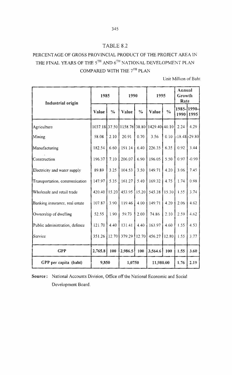
345

TABLE 8.2

PERCENT AGE OF GROSS PROVINCIAL PRODUCT OF THE PROJECT AREA IN

THE FINAL YEARS OF THE 5TH AND 6TH NATIONAL DEVELOPtv1ENT PLAN

COMPARED WITH THE 7TH PLAN

Unit Million of Baht

Annual 1985 1990 1995 Growth

Industrial origin Rate

Value ~yo Value ~yo Value 0/0 1985- 1990-1990 1995

Agriculture 1037.18 37.50 1158.76 38.80 1429.40 40.10 2.24 4.29

Mining 58.08 2.10 20.91 0.70 3.56 0.10 -18.48 -29.80

Manufacturing 182.54 6.60 191.14 6.40 226.35 6.35 0.92 3.44

Construction 196.37 7.10 206.07 6.90 196.05 5.50 0.97 -0.99

Electricity and water supply 89.89 3.25 104.53 3.50 149.71 4.20 3.06 7.45

Transportation, communication 147.97 5.35 161.27 5.40 169.32 4.75 1.74 0.98

Wholesale and retail trade 420.40 15.20 453.95 15.20 545.38 15.30 1.55 3.74

Banking insurance, real estate 107.87 3.90 119.46 4.00 149.71 4.20 2.06 4.62

Ownership of dwelling 52.55 1.90 59.73 2.00 74.86 2.10 2.59 4.62

Public administration, defence 121. 70 4.40 131.41 4.40 163.97 4.60 1.55 4.53

Service 351.26 12.70 379.29 12.70 456.27 12.80 1.55 3.77

epp 2,765.8 100 2,986.5 100 3,564.6 100 1.55 3.60

GPP per capita (baht) 9,850 1,0750 11,980.00 1.76 2.19

Source: National Accounts Division, Office off the National Economic and Social

Development Board.

346

Table 8.3 breaks down in the total GPP of Surat Thani province for the year

) 985 and 1996. Comparative analysis of the data reveals the following interesting points:

1. Agricultural sector of Surat Thani province contributed 33.80,34.6 and 34.2

percent to the total GPP of the province in 1985, 1990 and 1995 respectively. This

indicates that the agricultural sector plays a critical role in the economy of Surat Thani

province. Moreover, comparison of the 1990 data with that of 1995 data disclose that, in

spite of the increase in net GPP, the agricultural sector's contribution to the total GPP

actually increased.

2. Growth of other economic sectors has slightly reduced the importance of the

agricultural sector in Surat Thani. Electricity and water supply, public administration and

defense, banking insurance and real estate, services, and wholesale and retail trade were

the sectors which are growing at a higher rate than the previous year.

3. The results of analysis of the economic base of the province in the project

area clearly indicate that Surat Thani had a stronger economy. It enjoyed higher economic

growth in other non-agricultural sectors and attracted higher investment in wholesale,

service and public physical infrastructures.

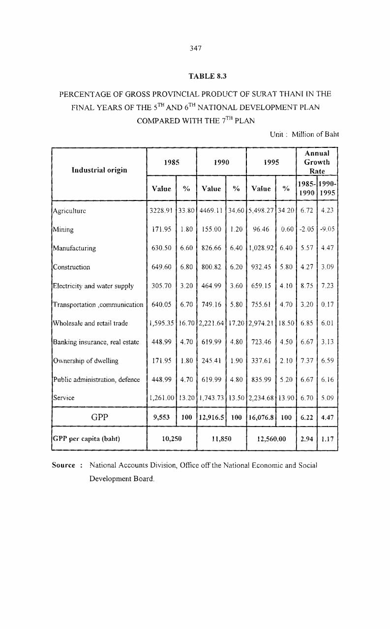
347

TABLE 8.3

PERCENTAGE OF GROSS PROVINCIAL PRODUCT OF SURAT THANI IN THE

FINAL YEARS OF THE 5TH AND 6TH NATIONAL DEVELOPMENT PLAN

COMP ARED WITH THE 7TH PLAN

Unit: Million of Baht

Annual 1985 1990 1995 Growth

Industrial origin Rate

Value °Al Value % Value (y«, 1985- 1990-1990 1995

Agriculture 3228.91 33.80 4469.11 34.60 5,498.27 3420 6.72 4.23

Mining 171. 95 1.80 155.00 1.20 96.46 0.60 -2.05 -9.05

Manufacturing 630.50 6.60 826.66 6.40 1,028.92 6.40 5.57 4.47

Construction 649.60 6.80 800.82 6.20 932.45 5.80 4.27 3.09

Electricity and water supply 305.70 3.20 464.99 3.60 659.15 4.10 8.75 7.23

Transportation ,communication 640.05 6.70 749.16 5.80 755.61 4.70 3.20 0.17

Wholesale and retail trade 1,595.35 16.70 2,221.64 17.20 2,974.21 18.50 6.85 6.01

Banking insurance, real estate 448.99 4.70 619.99 4.80 723.46 4.50 6.67 3.13

Ownership of dwelling 171.95 1.80 245.41 1.90 337.61 2.10 7.37 6.59

Public administration, defence 448.99 4.70 619.99 4.80 835.99 5.20 6.67 6.16

Service 1,261.00 13.20 1,743.73 13.50 2,234.68 13.90 6.70 5.09

GPP 9,553 100 12,916.5 100 ]6,076.8 100 6.22 4.47

GPP per capita (baht) 10,250 11,850 12,560.00 2.94 1.17

Source National Accounts Division, Office off the National Economic and Social

Development Board.

348

2. Evaluation of Actual Positive Benefits

2.1 General Background

Evaluation of actual positive benefits involves asseSSIng benefits of

multipurpose components in various aspects, which are interrelated. Evaluation In this

sense attempts to assess the overall impact of the project by means of benefit-cost analysis

technique. The benefits of the project are the values of incremental outputs of goods and

services made possible by the project.

2.2 Objectives

Objectives of this study aspect include the following:

(1) To estimate demand for electricity and damage due to electricity

interruption.

(2) To evaluate the actual positive benefits after the project implementation

and compare them with the estimated values before the project

construction;

(3) To identify all significant changes In benefits from the previously

estimated;

(4) To assess the multipurpose water resource development as previously

estimated.

2.3 Methodology of Study

To fulfill the above objectives, the following methodologies are adopted.

349

For the first objective, data and information were collected from 12 selected

industrial and service units utilizing pretested interview schedules. Information collected

relate 10 number of workers per industrial unit, labour per hour, value of product

produced per hour, cost of electricity per hour, damages due to electricity interruption per

hour, ability to generate own electricity, and cost of fuel for generating own electricity per

hour. Damages due to electricity interruption include two components; viz; direct damages

and indirect damages. Direct damages consist of loss in quantity and quality of product

outputs and storable inputs during electricity interruption. Indirect damage considered here

is only labour cost, which is the cost of non-storable input.

In regard to the second objective, benefits from hydropower, irrigation, water

supply, flood control, fisheries development, transportation and navigation, salinity and

water pollution control, tourism, health improvement, and resettlement were evaluated.

The data and information used in the evaluation of these benefits were obtained both from

primary and secondary sources. The methods used in evaluating the various components

were already described in Chapter 1.

By such methods, all significant changes in benefits from the project after

implementation from the previously estimated benefits can be identified. This fulfils the

third objective. Then, the last objective involving assessment of the multipurpose water

resource development as previously estimated can be achieved. The results of the study are

presented in four parts in the following paragraphs.

350

2.4 Results of the study

2.4.1 Demand for Electricity and Damage Due to Electricity Interruption

A field survey was conducted in June 1997 to give general picture on demand

for electricity as well as damages due to electricity interruption for selected industries and

services. The results of the survey are presented in Table 8.4.

From the 12 types of industrial units and services surveyed, it was found that

demand for electricity in terms of cost of electricity per hour ranged from 8 to 833 bahts

per hour. Four out of 12 of them are able to generate their own electricity when there is an

interruption of electricity supply from PEA The cost of fuel for generating their own

electricity ranges from 84 to 700 bahts per hour.

Value of product produced per hour for each industrial or service unit varies

considerably, ranging from only 60 to 22,220 bahts. Utilizing the value of product

produced per hour and cost of electricity per hour, factor share of electricity for each

industrial or service unit can be computed. Ice making industry which uses only few and

cheap inputs has a high factor share of electricity of about 82 percent while food canning

industry which uses expensive inputs has very low factor share of electricity,

approximately 1 percent. In general, factor share of electricity is about 6 percent, which

means that for every 100 bahts of value of product produced 6 bahts will be for electricity

cost.

Damages due to electricity interruption include two components: direct damage

and indirect damages. Direct damages were found only for ice making industry at the rate

of 3,000 bahts per hour. This damage was estimated from the fact that when there is no

351

electricity for one hour, the temperature of water that is about to become ice rises and it

takes about 3 hours for that water to resume the previous temperature. There is no direct

damage for the other 11 industrial units since the inputs (except labour) used by them can

be stored without much change quality until electricity is supplied again.

In this study, labour costs are considered as indirect damages. From worker's

point of view, labour cost paid by the owners of industrial units is the worker's revenue.

When there is an electricity interruption, the production process stops and workers cannot

earn their income during that period of time. The reduction in this income (or labour cost

from the point of view of the owner of industry) is, therefore, treated as indirect damage

due to electricity interruption. It ranges from 15 to 2,580 bahts per hour per industrial unit.

Combining the direct and indirect damages together total damages due to

electricity interruption are obtained and is presented in column 7 of Table 8.4. Ice making

industry has the largest total damage of 3,079 bahts per hour compared with 15 bahts per

hour for hair dressing service.

2.4.2 Evaluation of Actual Positive Benefits

As mentioned in section 2.3, eleven components of benefits are to be evaluated

as shown in Table 8.5. Some prices used in the evaluation of actual positive benefits after

the project implementation were not 1996 price, which was the price used in the estimation

of benefits before project implementation. Therefore, to make them comparable, the post­

evaluation benefits have to be converted to the benefits at 1987 price.

352

TABLE 8.4

DAMAGE DUE TO ELECTRICITY INTERRUPTION FOR SELECTED INDUSTRIES

AND SERVICE

Type of industries

and services

1. Fish meal

2. Saw mill

3. Rubber smokehouse

4. Mining

5. Ice making

6. Cold storage

7. food canning

8. Coconut oil refinery

9 . Welding shop

10. Hair dressing

11. Movie theatre

12. Restaurant

~ 'i: ..... '" = "0

= ,.

-.. ...... --

62

58

226

20

30

120

340

15

10

12

10

155 4,540 154 3.39

286 9,240 212 2.29

560 16,768 832 4.96

215 4,720 265 5,61

79 1,015 833 82.0

680 na 372 na

2,580 22,220 221 1.0

80 3,250 142 4.37

200 320 28 8.75

15 60 8 13.33

350 na 135 na

80 na 60 na

Notes na denotes not available.

Source Survey data

155 Yes 145

286 No

560 No.

255 No.

3,000 3,079 No.

680 Yes 84

2,580 Yes 220

80 No

200 No.

15 No.

350 Yes. 700

80 No.

353

TABLE 8.5

SOURCE OF DATA AND INFORMATION AND PRICE USED IN THE VALUATION

OF BENEFITS

Component off benefit to Source of data & information Price used in the

be evaluated used in the benefit evaluation of benefit

Hydropower Section 5.3 of Chapter VI 1996 price

Irrigation Section 3.3.3 of Chapter VI 1995 price

Water supply Section 3.3.2 of Chapter VI 1996 price

Flood protection Section 6.3 of Chapter VI 1996 price

Fisheries development Section 3 of Chapter V 1996 price

Transportation and

Navigation Section 4 of Chapter VI 1987 price

Salinity and water Section 8.4 of Chapter IV 1996 price

pollution control

Forestry Section 4.5 of Chapter V 1987 price

Tourism Section 4.9 of Chapter VII 1996 price

Health improvement Section 3 of Chapter VII 1995 price

Resettlement Section 2 of Chapter VII 1987 price

Twelve percent interest rate, which was adopted in estimation of benefits

before project construction, and has been the dominant rate of interest of government

bonds, is used in discounting the benefit stream. Since the construction of Rajjaprabha dam

began in 1980, and its operation commenced in 1987 and with the assumption of 50 years

354

project life, the stream of benefits at 1987 price from 1987 to 2037 are discounted to 1987

in this study.

The results of the evaluation of actual positive benefits are presented following

the order listed in section 2.3 of this chapter.

(1) Benefits from Hydropower

From the data and information obtained from section 5.3 of Chapter VI. the

hydropower benefit stream at 1996 price is computed :md that is discounted at the rate of

12 percent. The discounted hydropower beneftts are presented in Table 8.6. The present

worth of hydropower benefits amounts to 1650.10 million bahts.

(2) Benefits from Irrigation

The computation of benefits from irrigation is based on the data and

information from section 3.2.3 of Chapter VI. The estimated irrigation benefit stream at

1995 price is fint computed. Then it is discounted at the rate of 12 percent. The discounted

benefits from 1987 to 2037 are presented in Table 8.7. The estimated present worth of

benefits from irrigation 1,482.78 million bahts.

(3) Benefits from Water Supply

In this study costs of using groundwater as a substitute for raw water from

Phum Duang river are considered as benefits from water supply. It is estimated in section

3.3.2 of Chapter VI. The results of the estimation are presented in Table 8.8. The water

supply benefit stream, are converted to water supply benefit stream at 1987 price. Then it

355

is discounted by 12 percent. Ths discounted benefits are calculated and that comes to

approximately 131.21 million bahts.

(4) Benefits from Flood Protection

Flood protection benefit stream at 1996 pnce is assessed in section 6.3 of

Chapter VI as presented in Table 8.9. As in the case of other benefit streams it is converted

to benefits at 1987 price. This stream of benefits is discounted using 12 percent

discounting factor. That forms the discounted flood protection benefits. The estimated

present worth of flood protection benefits come to about 216.26 million bahts.

(5) Benefits from Fisheries Development

In 1980 it was estimated that the standing crops of fish in the proposed

reservOIr area and in the downstream area were 39.4 and 8.8 kilograms per ra1,

respectively. The standing crops of fish in 1996 as estimated in section 3 of Chapter V is

6.5 kilograms per rai in the reservoir area and 8.8 kilograms per rai in the downstream

area. These standing crops in 1996 are assumed to represent the maximum sustainable

yields. It was also assumed that the yields have increased linearly starting from 1988 when

the reservoir had stored water for one year.

With these estimated increase in yield from an average reservoir surface area of

17,800 ha, average downstream water surface area of 15,000 ha, and average fish price of

35 bahts per kilogram in 1996, the fisheries development benefit stream at 1996 price is

estimated and presented in Table 8.10. This benefit stream does not include downstream

loss during the construction period and loss of migratory species since they are considered

as negligible and insignificant from economic viewpoint. Benefits of aquaculture usmg

356

water from the project are low In potential therefore; they are also excluded from

computation of benefits.

The benefit stream at 1996 price is converted to benefit stream at 1987 price

and presented in Table 8.10. From this benefit stream, the present worth of fisheries

development benefits using 12 percent discount rate are estimated approximately 300.76

million bahts, 237.6 million bahts from the reservoir fisheries development and another

63.16 million bahts from the downstream fisheries development.

(6) Benefits from Transportation and Navigation

The study in section 4 of Chapter VI indicates that since the implementation of

the project there has been no detectable change in land transportation, and the

development potential for navigation. Therefore, estimation of benefits of this component

involves only the cost of relocating road, the cost of using relocated road, the cost of using

old road, and maintenance costs for the relocated road and the old road.

It is reported that cost of the construction work with respect to road relocation

was 70,800,000 bahts. It was also indicated that the relocated road is 20 kilometers longer

than the old one. With the data on average daily traffic volume from section 4 of Chapter VI,

the estimated traffic volume per day is made as shown in Table 8.11. It should be noticed

that the allowable maximum traffic volume per day is 8,000 (Team Consulting Co.Ltd

1980). Therefore, from year 2015 onwards the traffic volume is taken as 8,000 per day.

The data and information obtained from Highways Department reveal that (1) at

the beginning of every eighth year there is a special road maintenance, and the maintenance

cost is estimated at 60 bahts per square meter (1987 price) for highway No. 401, (2) routine

357

maintenance costs ill bahts per kilometer per year at 1987 pnce for this highway are

18,167+0.0828 average daily traffic volume (ADT) for good road condition; 14,522+0.0663

ADT for fair road condition; and 10,878+0.0497 ADT for poor road condition.

Based on total road user operating cost at the speed of 60 kilo meters per hour

which is 5.28 bahts per kilometer and the data mentioned above, transportation benefit

stream at 1987 price is estimated as shown in Table 8.11. With 12 percent discount rate,

therefore, the present worth of transportation benefit comes to -228.03 million bahts.

(7) Benefits from Salinity and Water Pollution Control

The benefits from salinity and water pollution control are negligible as

mentioned in section 8.4 of Chapter IV.

(8) Benefits from Forestry

The results of the study of section 4.5 of Chapter V reveal that (1) Since the

project was implemented, deforestation and illegal logging have decreased, and this

decrease is estimated at 0.49 million bahts per year, (2) benefit from logging of vegetation

in the resettlement area about 2.7 million bahts (1980). (3) benefits from timber logging in

the overall reservoir about 324.4 million bahts. (4) damages from uncut forests about 18.01

million baths in the first year to about 72.53 million baths in the 50th year.

These gain and losses are valued at 1987 price. With these results of the study,

forestry benefit stream is estimated as shown in Table 8.12. Then, the present worth of

forestry benefits is computed using 12 percent discount rate. It is approximately - 370.65

million bahts.

358

(9) Benefits from Tourism

The number of people who visited the Rajjaprabha dam was 20,519 in 1987,

61,662 in 1988, and 88,048 in 1996. The number ofpeopJe who expected to visit the dam

is also estimated to be about 92, 101, 112, and 120 thousands in, 2000, 2015, 2020 and

2030, respectively. With these data, the estimation of number of visitors is further made for

the periods of 2000-20 10, 2011-2020 and 2021-2030.

On the basis of a benefit of 105 bahts per visitor in 1996 (estimated in section

4.9 of Chapter VII), benefit from tourism at 1996 price is estimated and that is shown in

Table 8.13. This benefit stream is then converted to the benefit stream at 1987 price. With

12 percent discount factor, the present worth of benefits from tourism is estimated to be

approximately 176.75 million bahts.

(10) Benefits from Health Improvement

Benefits from health improvement include two components, i.e., increase in

earning of person and decrease in cost of health care. The increase in earning is estimated

by mUltiplying the increase in number of survivals of infants and children until they

become adults by average income per adult. The decrease in cost of health care is the

product of the decrease in number of patients and cost of medical care per person. It is

indicated in section 3 of Chapter VII that:

(1) Total number of household in 1996 in Pattana village and Khoa Sok

village, which is the control village were 386 and 225 respectively and the

average number of person per household were 4.3 and 5.4 respectively.

359

(2) The percentage of infants, children, and adults were 20, 25, 55 in Pattana

village and 19, 27, 54 in Ban Khoa Sok respectively

(3) Percentage of people who were sick during the last 12 months at the time

of survey was 63 and 68 in Pattana village and Khoa Sok village,

respectively.

Data and information in section 2 of Chapter VII that are relevant for

estimation of benefits from health improvement reveal that:

(1) The average population growth rate in Pattana village and Khoa Sok

village was 0.2 and 0.3 per cent per year respectively.

(2) The average annual income per household in 1996 was 54,210 bahts in

Pattana village and 48,500 bahts in Khoa Sok village.

(3) The average costs of medical care per household in 1996 were 1,500 bahts

for both the villages.

Based on the data and information mentioned above:

(1) It is estimated that the average earning per person, which is the average

income per household divided by average number of adults per household,

was 10,050 and 8,640 bahts per year at 1996 price in Pattana village and

Khoa Sok village respectively.

(2) It is estimated that the average cost of medical care per person, which is

the average cost of medical care per household divided by the number of

person per household, are 250 bahts per year at 1996 price in both the

villages.

360

(3) Estimation of population during 1987-1995 and 1997-2037 is made based

on (i) the average population growth rate of 0.57 percent per year, (ii) the

total population of 26 in Pattana village, 18 in Khoa Sok village in 1996.

The children until they become adults is made based on (i) percentage of

infants and children as indicated in section 3 of Chapter VII (ii) mortality

rate as indicated in section 3 of Chapter VII. The results of the estimation

are presented in Table 8.14

(4) Benefits from the decrease in cost of health care are estimated based on;

(a) percentage of people who were sick as indicated in section 3 of

Chapter VII (b) population as estimated ( c) the average cost of medical

care per person as mentioned above. The results of the estimation are

presented in Table 8.15

(5) Benefits from increase in earning are estimated based on; (a) cumulative

increase in survivals of infants and children until they become adults, and

(b) the average earning per person mentioned above. The results of the

estimation are presented in Table 8.16.

Thus, health improvement benefit stream at 1996 pnce can be derived by

combining the stream of benefits from decrease in cost of health care with the stream of

benefits from increase in earning as shown in Table 8.] 7. The health improvement benefit

stream at 1996 price is converted to the benefit stream at 1987 price. With 12 percent

discount rate, the present worth of benefits from health improvement is approximately

89.14 million bahts.

361

(11) Benefits from ResettJement

Benefit from resettlement is the difference between post-resettled household

income and pre-resettled household income. The post-resettled income and pre-resettled

income per household at 1996 price are already presented in section 2 of Chapter VII. The

socio-economic study of farmers in resettlement areas also indicated that there were 385

households in Pattana village.

Considering the post-resettled and pre-resettled incomes, it is found that there

are 4 sources of income. They are (i) rubber (inside and outside resettled area), (ii) fishery

(iii) rubber tapping and (iv) hired labor. Benefits from resettlement originated from these 4

sources of income and they are estimated as follows.

(1) Rubber in resettled area: There are rubber plantations in the resettlement

area in Pattana village. The average income from this rubber in 1996 was 36,400 bahts per

household in Pattana village and 24,800 bahts per household in Khoa Sok village.

Information from the Office of Rubber Replantation Fund indicates that latex can be

tapped from rubber trees at the age of 7 to 20 years. The indices of yield are 28 at the age

of 7 years, 44 at the age of 8 years, 66 at the age of 10 years, 78 at the age of 11-15 years,

85 at the ages of 16 to 20 years, and 83 at the ages of 23 to 25 years. Based on these data

and the number of household mentioned earlier, stream of benefits from rubber in resettled

area is estimated.

(2) Fishery: Only a part of the people in Pattana village earns their incomes

from fishery. After they moved to stay in the resettlement area, income from fishery has

362

increased by 6,800 bahts per household per year. Therefore, it is estimated that

resettlement benefit derived from fishery is about 4.58 million bahts per year.

(3) Rubber tapping: After moving to the resettlement area, income from

rubber tapping of the people in Pattana village has increased by 1,650 bahts per household

per year, while in Khoa Sok village the increase was 1,705 bahts per household per year.

Thus, resettlement benefit derived from rubber tapping is estimated at about -0.02 million

bahts per year.

(4) Hired labor: With the same procedure used in estimating resettlement

benefits originated from fishery and rubber tapping, resettlement benefits originated from

hired labor is estimated. It is about 0.80 million bahts per year.

Combining all the 4 sources of benefit together the overall resettlement benefit

stream at 1984 price is obtained as shown in Table 8.18. This stream of benefits is

converted to benefit stream at 1987 price. With 12 percent discount rate, the present worth

of resettlement benefit is estimated at about 152.25 million bahts.

363

TABLE 8.6

HYDRO POWER BENEFIT STREAM AT 1996 PRICE AND TWEL YE PERCENT

DISCOUNTED HYDRO POWER BENEFIT

.... ~

o U

.... ~

o U

Unit: Million of Baht

1981 56.000 0.000 -56.000 -306.520 20lO 50.000 775.500 725.500 148.452 1982 76.000 0.000 -76.000 -371.421 2011 103.000 775.500 672.500 122.863

1983 396.000 0.000 -396.000 -1727.943 2012 50.000 775.500 725.500 118.345

1984 690.000 0.000 -690.000 -2688.223 2013 50.000 775.500 725.500 105.665

1985 1189.000 0.000 -1189.000 -4135.996 2014 50.000 775.500 725.500 94.344

1986 130.000 0.000 -130.000 -403.760 2015 50.000 775.500 725.500 84.235

1987 39.000 150.700 1l1.700 309.753 2016 50.000 775.500 725.500 75.210

1988 39.000 178.400 139.400 345.149 2017 50.000 775.500 725.500 67.152

1989 36.000 258.200 222.200 491.213 2018 62.000 775.500 713.500 58.965

1990 146.000 337.600 191.600 378.184 2019 58.000 775.500 717.500 52.943

1991 145.000 406.300 261.300 460.500 2020 105.000 775.500 670.500 44.174

1992 45.000 500.400 455.400 716.581 2021 100.000 775.500 675.500 39.735

1993 45.000 566.700 521.700 732.951 2022 62.000 775.500 713.500 37.474

1994 50.000 643.100 593.lO0 743.985 2023 50.000 775.500 725.500 34.021

1995 50.000 713.000 663.000 742.560 2024 50.000 775.500 725.500 30.376

1996 50.000 775.500 725.500 725.S00 2025 50.000 77S.500 725.500 27.122

1997 50.000 653.700 603.700 539.018 2026 50.000 775.500 725.S00 24.216

1998 50.000 775.500 725.500 578.364 2027 50.000 775.500 725.500 21.621

1999 50.000 775.500 725.500 516.397 2028 50.000 775.500 725.500 19.305

2000 50.000 775.500 725.500 461.068 2029 50.000 775.500 725.500 17.236

2001 50.000 77S.500 72S.S00 411.668 2030 SO.OOO 77S.500 725.500 15.390

2002 50.000 775.500 725.500 367.561 2031 50.000 77S.500 725.500 13.741

2003 SO.OOO 775.500 725.500 328.179 2032 50.000 775.500 725.500 12.268

2004 179.000 775.500 S96.500 240.916 2033 SO.OOO 775.500 725.500 10.954

2005 267.000 775.500 508.500 183.370 2034 50.000 775.500 725.500 9.780

2006 303.000 775.500 472.500 152.132 2035 50.000 775.500 725.500 8.732

2007

2008

2009

89.000 775.500 686.500

50.000 775.500 725.500

50.000 775.500 725.500

197.352 2036 50.000 775.500 725.500 7.797

186.218 2037 50.000 775.500 725.500 6.961

166.266 SUM 6,060.0 36,203.629,943.6 1,650.1

364

TABLE 8.7

IRRIGATION BENEFIT STREAM AT 1996 PRICE

AND TWELVE PERCENT DISCOUNTED IRRIGATION BENEFIT

Unit: Million of Baht

... (lJ (lJ ... (lJ (lJ - e.;: ~ :s "0 ... e.;: .::! :s "0

'" (lJ 4,) ·c - (lJ ~ (lJ (lJ I. ~ (lJ 0 :s ::: Co ~ - 0 :s ;: c. -I. U ::: CIJ-..:>

> ~ ;: I. U ::: (lJ-..:> > ~ :::

~ _ Q :s ~ ... e :s

4,) -; 4,) ..QO'I ::: M 0 (lJ -; 4,) ..QO'I ::: M 0 >- > >- > ... CIJ -0'1 CIJ ...... ~ ... CIJ -0'1 ~ ...... ~

0 ~ .5- '" '" 0 ~ .5- '" .~ Q,I .. Q,I E-

o _ I. ~ E- o ... I. ~ E--< ~ E--< ~

1980 26.000 0.000 -26.000 -142.313 2010 12.000 199.000 187.000 34.164 1981 59.000 0.000 -59.000 -288.340 2011 13.000 199.000 186.000 30.341

1982 86.000 0.000 -305.445 -305.445 2012 32.000 199.000 167.000 24.323

1983 226.000 5.000 -221.000 -861.011 2013 48.000 199.000 151.000 19.636

1984 94.000 14.000 -80.000 -278.284 2014 120.000 199.000 79.000 9.172

1985 62.000 34.000 -28.000 -86.964 2015 36.000 199.000 163.000 16.898

1986 86.000 60.000 -26.000 -72.100 2016 16.000 199.000 183.000 16.938

1987 28.000 9l.000 63.000 155.986 2017 12.000 199.000 187.000 15.454

1988 12.000 126.000 114.000 252.018 2018 12.000 199.000 187.000 13.798

1989 12.000 150.000 138.000 272.388 2019 12.000 199.000 187.000 12.320

1990 12.000 176.000 164.000 289.024 2020 12.000 199.000 187.000 11.000

1991 12.000 178.000 166.000 261.204 2021 12.000 199.000 187.000 9.821

1992 12.000 180.000 168.000 236.028 2022 12.000 199.000 187.000 8.769

1993 12.000 186.000 174.000 218.266 2023 12.000 199.000 187.000 7.830

1994 ,12.000 197.000 185.000 207.200 2024 13.000 199.000 186.000 6.953

1995 12.000 195.000 183.000 183.000 2025 15.000 199.000 184.000 6.142

1996 13.000 199.000 186.000 166.071 2026 13.000 199.000 186.000 5.543

1997 14.000 199.000 185.000 147.481 2027 12.000 199.000 187.000 4.976

1998 15.000 199.000 184.000 130.968 2028 12.000 199.000 187.000 4.443

1999 14.000 199.000 185.000 1l7.571 2029 12.000 199.000 187.000 3.967

2000 16.000 199.000 183.000 103.839 2030 12.000 199.000 187.000 3.542

2001 15.000 199.000 184.000 93.220 2031 12.000 199.000 187.000 3.162

2002 12.000 199.000 187.000 84.589 2032 12.000 199.000 187.000 2.823

2003 12.000 199.000 187.000 75.526 2033 12.000 199.000 187.000 2.521

2004 12.000 199.000 187.000 67.434 2034 12.000 199.000 187.000 2.251

2005 12.000 199.000 187.000 60.209 2035 13.000 199.000 186.000 1.999

2006 12.000 199.000 187.000 53.758 2036 14.000 199.000 185.000 1.775

2007 12.000 199.000 187.000 47.998 2037 13.000 199.000 186.000 l.594

2010 12.000 199.000 187.000 34.164 SUM 1,484.0 9,950.0 8,466.0 1482.78

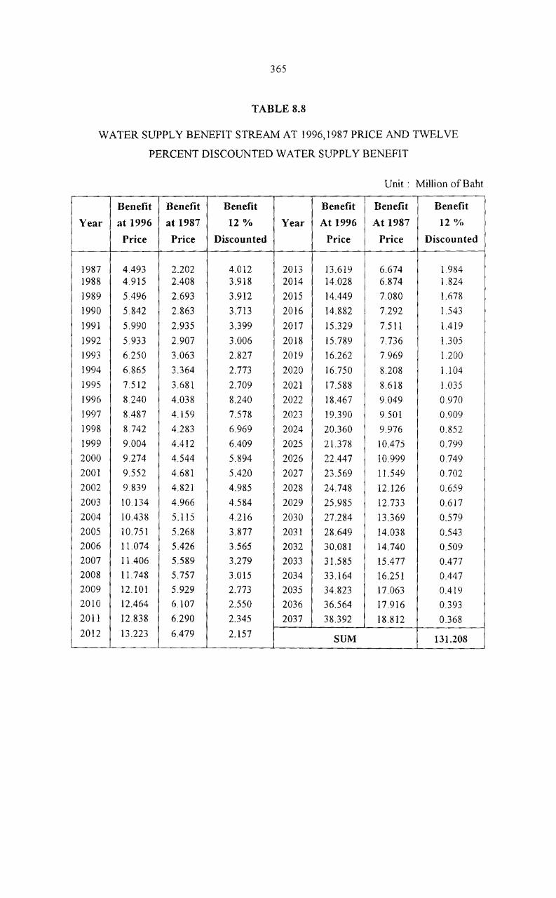
365

TABLE 8.8

W ATER SUPPLY BENEFIT STREAM AT 1996,1987 PRICE AND TWEL YE

PERCENT DISCOUNTED WATER SUPPLY BENEFIT

Unit: Million of Baht

Benefit Benefit Benefit Benefit Benefit Benefit

Year at 1996 at 1987 12 % Year At 1996 At 1987 12 0;(1

Price Price Discounted Price Price Discounted

1987 4.493 2.202 4.012 2013 13.619 6.674 1.984 1988 4.915 2.408 3.918 2014 14.028 6.874 1.824

]989 5.496 2.693 3.912 2015 14.449 7.080 1.678

1990 5.842 2.863 3.713 2016 14.882 7.292 1.543

199] 5.990 2.935 3.399 2017 ]5.329 7.511 1.419

1992 5.933 2.907 3.006 2018 15.789 7.736 1.305

1993 6.250 3.063 2.827 20]9 16.262 7.969 1.200

1994 6.865 3.364 2.773 2020 16.750 8.208 1.104

1995 7.512 3.681 2.709 2021 17.588 8.618 1.035

]996 8.240 4.038 8.240 2022 18.467 9.049 0.970

1997 8.487 4.159 7.578 2023 19.390 9.501 0.909

1998 8.742 4.283 6.969 2024 20.360 9.976 0.852

1999 9.004 4.412 6.409 2025 21.378 10.475 0.799

2000 9.274 4.544 5.894 2026 22.447 10.999 0.749

2001 9.552 4.681 5.420 2027 23.569 1] .549 0.702

2002 9.839 4.821 4.985 2028 24.748 12.126 0.659

2003 10.134 4.966 4.584 2029 25.985 12.733 0.617

2004 10.438 5.115 4.216 2030 27.284 13.369 0.579

2005 10.751 5.268 3.877 2031 28.649 14.038 0.543

2006 11.074 5.426 3.565 2032 30.081 14.740 0.509

2007 11.406 5.589 3.279 2033 31.585 15.477 0.477

2008 11.748 5.757 3.015 2034 33.164 16.251 0.447 2009 12.101 5.929 2.773 2035 34.823 17.063 0.419 2010 12.464 6.107 2.550 2036 36.564 17.916 0.393

2011 12.838 6.290 2.345 2037 38.392 18.812 0.368

2012 13.223 6.479 2.157 SUM 131.208

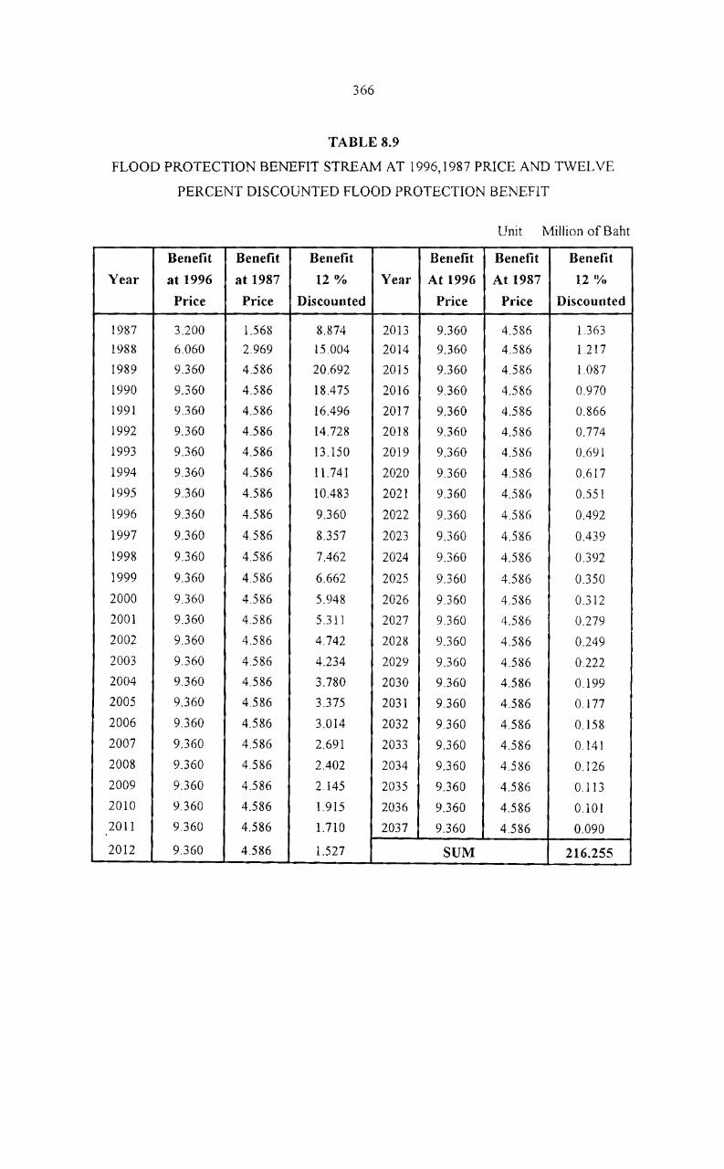
366

TABLE 8.9

FLOOD PROTECTION BENEFIT STREAM AT 1996,1987 PRICE AND TWELVE

PERCENT DISCOUNTED FLOOD PROTECTION BENEFIT

Unit Million ofBaht

Benefit Benefit Benefit Benefit Benefit Benefit

Year at 1996 at 1987 12 % Year At 1996 At 1987 12 {Y«.

Price Price Discounted Price Price Discounted

1987 3.200 1.568 8.874 2013 9.360 4.586 1.363

1988 6.060 2.969 15.004 2014 9.360 4.586 1.217

1989 9.360 4.586 20.692 2015 9.360 4.586 1.087

1990 9.360 4.586 18.475 2016 9.360 4.586 0.970

1991 9.360 4.586 16.496 2017 9.360 4.586 0.866

1992 9.360 4.586 14.728 2018 9.360 4.586 0.774

1993 9.360 4.586 13.150 2019 9.360 4.586 0.691

1994 9.360 4.586 11.741 2020 9.360 4.586 0.617

1995 9.360 4.586 10.483 2021 9.360 4.586 0.551

1996 9.360 4.586 9.360 2022 9.360 4.586 0.492

1997 9.360 4.586 8.357 2023 9.360 4.586 0.439

1998 9.360 4.586 7.462 2024 9.360 4.586 0.392

1999 9.360 4.586 6.662 2025 9.360 4.51)6 0.350

2000 9.360 4.586 5.948 2026 9.360 4.586 0.312

2001 9.360 4.586 5 .311 2027 9.360 4.586 0.279

2002 9.360 4.586 4.742 2028 9.360 4.586 0.249

2003 9.360 4.586 4.234 2029 9.360 4.586 0.222

2004 9.360 4.586 3.780 2030 9.360 4.586 0.199

2005 9.360 4.586 3.375 2031 9.360 4.586 0.177

2006 9.360 4.586 3.014 2032 9.360 4.586 0.158

2007 9.360 4.586 2.691 2033 9.360 4.586 0.141

2008 9.360 4.586 2.402 2034 9.360 4.586 0.126

2009 9.360 4.586 2.145 2035 9.360 4.586 0.113

2010 9.360 4.586 1.915 2036 9.360 4.586 0.101

2011 9.360 4.586 1.710 2037 9.360 4.586 0.090

2012 9.360 4.586 1.527 SUM 216.255

367

TABLE 8.10

FISHERIES DEVELOPMENT BENEFIT STREAM AT 1996, 1987 AND TWEL YE

PERCENT DISCOUNTED FISHERIES DEVELOPMENT BENEFIT

Unit : Million of Baht

Benefit Benefit Benefit Benefit Benefit Benefit Year at 1996 at 1987 12 % Year At 1996 At 1987 12 <Yo

Price Price Discounted Price Price Discounted

1990 0.000 0.000 0 2014 27.000 13.230 3.511

1991 0.000 0.000 0 2015 27.000 13.230 3.135

1992 3.000 1.470 4.721 2016 27.000 13.230 2.799

1993 7.000 3.430 9.834 2017 27.000 13.230 2.499

1994 ]4.000 6.860 17.562 2018 27.000 13.230 2.23 I

1995 21.000 10.290 23.520 2019 27.000 13.230 1.992

1996 27.000 13.230 27.000 2020 27.000 13.230 1.779

1997 27.000 13.230 24.107 2021 27.000 13.230 1.588

1998 27.000 13.230 21.524 2022 27.000 13.230 1.418

1999 27.000 13.230 19.218 2023 27.000 13.230 1.266

2000 27.000 13.230 17.159 2024 27.000 13.230 1.130

2001 27.000 13.230 15.321 2025 27.000 13.230 1.009

2002 27.000 13.230 13.679 2026 27.000 13.230 0.901

2003 27.000 13.230 12.213 2027 27.000 13.230 0.805

2004 27.000 13.230 10.905 2028 27.000 13.230 0.7111

2005 27.000 13.230 9.736 2029 27.000 13.230 0.641

2006 27.000 13.230 8.693 2030 27.000 13.230 0.573

2007 27.000 13.230 7.762 2031 27.000 13.230 0.511

2008 27.000 13.230 6.930 2032 27.000 13.230 0.457

2009 27.000 13.230 6.188 2033 27.000 13.230 0.4011

2010 27.000 13.230 5.525 2034 27.000 13.230 0.364

2011 27.000 13.230 4.933 2035 27.000 13.230 0.325

2012 27.000 13.230 4.404 2036 27.000 13.230 0.290

2013 27.000 13.230 3.932 2037 27.000 13.230 0.259

2014 27.000 13.230 3.511 SUM 300.757

368

TABLE 8.11

ESTIMATE TRAFFIC VOLUME AND BENEFIT STREAM AT 1987 PRICE AND

TWELVE PERCENT DISCOUNTED TRANSPORTATION BENEFITS

Unit : Million of Baht

Benefit Benefit Benefit Benefit Benefit Benefit Year at 1996 at 1987 12%

Year At 1996 At 1987 12 IYI,

Price Price Discounted Price Price Discounted

1997 740 -70.800 -70.800 2013 6663 -20.000 -1.050

1988 785 -7.850 -7.009 2014 7329 -20.000 -0.938

1989 832 -7.850 -6.258 2015 8000 -20.000 -0.837

1990 918 -7.850 -5.587 2016 !WOO -20.000 -0.748

1991 974 -7.850 -4.9g9 2017 8000 -20.000 -0.608

1992 1033 -7.850 -4.454 2018 8000 -20.000 -0.596

1993 1096 -7.850 -3.977 2019 8000 -20.000 -0.532

1994 1163 -7.850 -3.551 2020 8000 -50.500 -1.200

1995 1234 -7.850 -3.170 2021 8000 -50.500 -1.071

1996 1309 -7.850 -2.831 2022 8000 -50.500 -0.956

1997 1450 -7.850 -2.527 2023 8000 -50.500 -0.854

1998 1595 -12.000 -3.450 2024 8000 -50.500 -0.762

1999 1755 -12.000 -3.080 2025 8000 -50.500 -0.681

2000 1930 -12.000 -2.750 2026 8000 -50.500 -0.608

2001 2123 -12.000 -2.455 2027 8000 -50.500 -0.543

2002 2335 -12.000 -2.192 2028 8000 -50.500 -0.485

2003 2569 -12.000 -1.957 2029 8000 -50.500 -0.433

2004 2826 -12.000 -1.748 2030 !WOO -50.500 -0.3g6

2005 3108 -12.000 -1.560 2031 8000 -50.500 -0.345

2006 3419 -12.000 -1.393 2032 8000 -50.500 -0.308

2007 3761 -12.000 -1.244 2033 8000 -50.500 -0.275

2008 4137 -12.000 -1.111 2034 8000 -50.500 -0.245

2009 4551 -20.000 -1.653 2035 8000 -50.500 -0.219

2010 5006 -20.000 -1.476 2036 8000 -50.500 -0.196

2011 5506 -20.000 -1.318 2037 8000 -50.500 -0.175

2012 6057 -20.000 -1.176 SUM -147.729

369

TABLE 8.12

FORESTRY BENEFIT STREAM AT 1987 PRICE AND TWELVE PERCENT

DISCOUNTED FORESTRY BENEFIT

Unit Million ofBaht

Benefit Benefit Benefit Benefit

Year at 1987 12 % Year at 1987 12 {YtJ

Price Discounted Price Discounted

1982 324.400 57l.704 2010 -106.930 -7.890 1983 9.360 14.728 2011 -106.930 -7.045

1984 9.360 13.150 2012 -106.930 -6.290

1985 9.360 1l.741 2013 -106.930 -5.616

1986 9.360 10.483 2014 -106.930 -5.014

1987 -18.010 -18.010 2015 -106.930 -4.477

1988 -18.010 -16.080 2016 -98.880 -3.696

1989 -18.010 -14.357 2017 -98.880 -3.300

1990 -18.010 -12.819 2018 -98.880 -2.947

1991 -18.010 -1l.446 2019 -98.880 -2.631

1992 -18.010 -10.219 2020 -98.880 -2.349

1993 -18.010 -9.124 2021 -98.880 -2.097

1994 -18.010 -8.147 2022 -98.880 -1.873

1995 -18.010 -7.274 2023 -98.880 -1.672

1996 -89.510 -32.278 2024 -98.880 -1.493

1997 -89.510 -28.820 2025 -98.880 -1.333

1998 -89.510 -25.732 2026 -85.650 -1.031

1999 -89.510 -22.975 2027 -85.650 -0.920

2000 -89.510 -20.513 2028 -85.650 -0.822

2001 -89.510 -18.316 2029 -85.650 -0.734 2002 -89.510 -16.353 2030 -85.650 -0.655

2003 -89.510 -14.601 2031 -85.650 -0.585 2004 -89.510 -13.037 2032 -85.650 -0.522 2005 -89.510 -11.640 2033 -85.650 -0.466 2006 -106.930 -12.415 2034 -85.650 -0.416 2007 -106.930 -11.085 2035 -85.650 -0.372 2008 -106.930 -9.897 2036 -72.530 -0.281

2009 -106.930 -8.837 2037 -72.530 -0.251

2010 -106.930 -7.890 -106.930 SUM -370.654

370

TABLE 8.13

TOURISM BENEFIT STREAM AT 1996, 1987 PRICE AND TWEL YE PERCENT

DISCOUNTED TOURISM BENEFITS

Unit : million of Baht

Benefit Benefit Benefit Benefit Benefit Benefit Year at 1996 at 1987 12% Year At 1996 At 1987 12 ·X.

Price Price Discounted Price Price Discounted

1987 1.240 1.240 3.439 2013 10.754 5.269 1.566 1988 2.010 2.010 4.977 2014 10.754 5.269 1.398

1989 6.240 6.240 13.795 2015 12.061 5.910 1.400

1990 6.230 6.230 12.297 2016 12.061 5.910 1.250

1991 5.420 5.420 9.552 2017 12.061 5.910 1.116

1992 5.850 5.850 9.205 2018 12.061 5.910 0.997

1993 6.670 6.670 9.371 2019 12.061 5.910 0.890

1994 8.250 8.250 10.349 2020 13.492 6.611 0.889

]995 9.142 9.410 10.239 202] 13.492 6.611 0.794

1996 9.245 4.738 9.245 2022 13.492 6.611 0.709

1997 9.245 4.530 8.254 2023 13.492 6.611 0.633

1998 9.245 4.530 7.370 2024 13.492 6.611 0.565

1999 9.245 4.530 6.580 2025 15.380 7.536 0.575

2000 9.623 4.715 6.116 2026 15.380 7.536 0.513

2001 9.623 4.715 5,460 2027 15.380 7.536 0.458

2002 9.623 4.715 4.875 2028 15.380 7.536 0.409

2003 9.623 4.715 4.353 2029 15.3 80 7.536 0.365

2004 9.623 4.715 3.887 2030 16.008 7.844 0.340

2005 10.339 5.066 3.728 2031 16.008 7.844 0.303

2006 10.339 5.066 3.329 2032 16.008 7.844 0.271

2007 10.339 5.066 2.972 2033 16.008 7.844 0.242

2008 10.339 5.066 2.654 2034 16.008 7.844 0.216

2009 10.339 5.066 2.369 2035 16.008 7.844 0.193

2010 10.754 5.269 2.200 2036 16.008 7.844 0172

2011 10.754 5.269 1.965 2037 16.008 7.844 0.154

2012 10.754 5.269 1.754 SUM 176.753

371

TABLE 8.14

ESTIMA nON OF POPULA nON DURING 1987-2037

Unit : In person

Year Khao Sok village Pattana village

Year Khao Sok village Pattana village

At 1996 at 1987 at 1996 at 1987

1987 1226 1568 2013 1307 1647

198R 1230 1571 2014 1310 1650

1989 1233 1574 2015 1312 1653

1990 1237 1577 2016 1315 1656

1991 1241 1581 2017 1317 J659

1992 1245 1584 2018 1320 1662

1993 124g 1587 2019 1323 1665

1994 1252 1590 2020 1325 1668

1995 1256 1593 2021 1328 1671

1996 1260 1596 2022 1331 1674

1997 1263 1600 2023 1333 1677

1998 1267 1603 2024 1336 1680

1999 1271 1606 2025 1339 1683

2000 1273 1609 2026 1341 1686

2001 1276 1612 2027 1344 1689

2002 1279 1615 2028 1347 1692

2003 1281 1618 2029 1349 1695

2004 1284 1621 2030 1352 1698

2005 1286 1623 2031 1355 170J

2006 1289 1626 2032 1357 1704

2007 1291 1629 2033 1360 1707

2008 1294 1632 2034 1363 1710

2009 1297 1635 2035 1366 1713

2010 1299 1638 2036 1368 1717

2011 1302 1641 2037 1371 1720

2012 1304 1644

372

TABLE 8.15

BENEFIT FROM DECREASE IN COST OF HEALTH CARE

Unit Million of Baht

Year Khao Sok Pattana

Year Khao Sok village Pattana village village village

1987 -6.616 -9.340 2013 -7.060 -9.825

1988 -6.642 -9.373 2014 -7.074 -9.843

1989 -6.662 -9.391 2015 -7.088 -9.861

1990 -6.682 -9.410 2016 -7.102 -9.X78

1991 -6.702 -9.429 2017 -7.116 -9.896

1992 -6.723 -9.448 2018 -7.131 -9.914

1993 -6.743 -9.467 2019 -7.145 -9.932

1994 -6.763 -9.486 2020 -7.159 -9.950

1995 -6.783 -9.505 2021 -7.173 -9.968

1996 -6.804 -9.524 2022 -7.188 -9.986

1997 -6.824 -9.543 2023 -7.202 -10.004

1998 -6.844 -9.562 2024 -7.217 -10.022

1999 -6.865 -9.5 81 2025 -7.231 -10.040

2000 -6.879 -9.598 2026 -7.245 -10.058

2001 -6.892 -9.615 2027 -7.260 -10.076

2002 -6.906 -9.633 2028 -7.275 -10.094

2003 -6.920 -9.650 2029 -7.289 -10.112

2004 -6.934 -9.668 2030 -7.304 -10.130

2005 -6.948 -9.685 2031 -7.318 -10.149

2006 -6.962 -9.702 2032 -7.333 -10.167

2007 -6.976 -9.720 2033 -7.348 -10.185

2008 -6.990 -9.737 2034 -7.362 -10.203

2009 -7.004 -9.755 2035 -7.377 -10.222

2010 -7.018 -9.772 2036 -7.392 -10.240

2011 -7.032 -9.790 2037 -7.406 -10.259

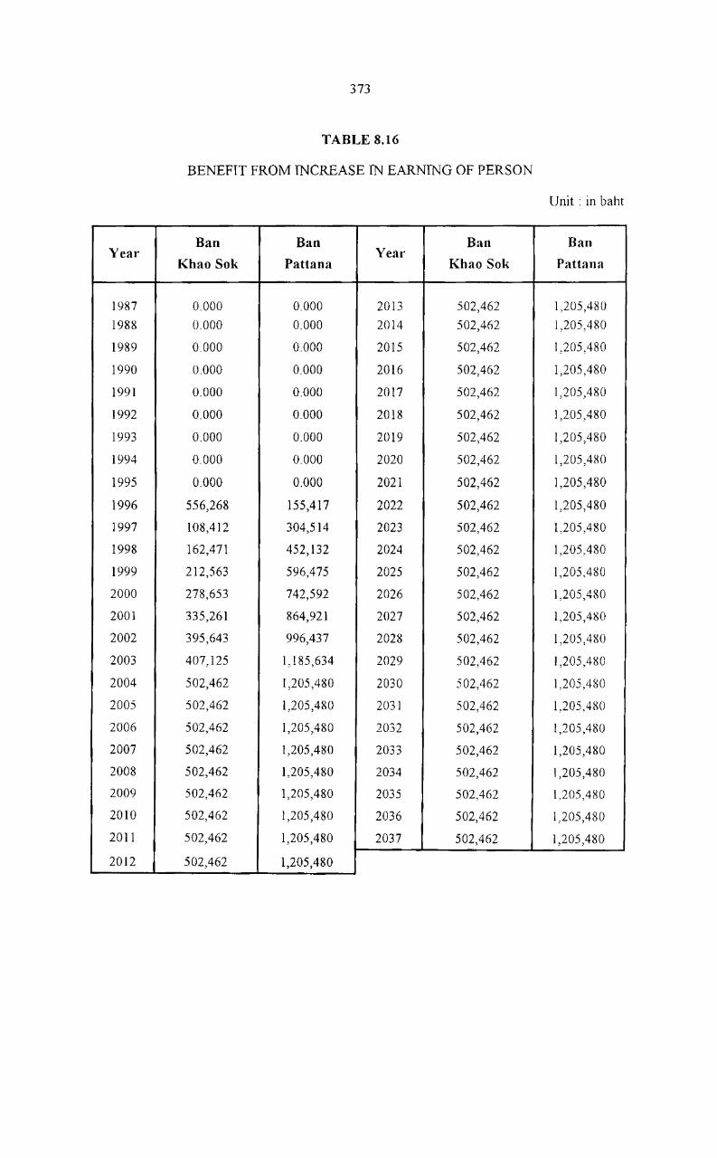
373

TABLE 8.16

BENEFIT FROM INCREASE IN EARNING OF PERSON

Unit: in baht

Ban Ban Ban Ban Year Year

Khao Sok Pattana Khao Sok Pattana

1987 0.000 0.000 2013 502,462 1,205,4S0

1988 0.000 0.000 2014 502,462 1,205,480

1989 0.000 0.000 2015 502,462 1,205,480

1990 0.000 0.000 2016 502,462 1,205,480

1991 0.000 0.000 2017 502,462 1,205,480

1992 0.000 0.000 2018 502,462 1,205,480

1993 0.000 0.000 2019 502,462 1,205,480

1994 0.000 0.000 2020 502,462 1,205,480

1995 0.000 0.000 2021 502,462 1,205,480

1996 556,268 155,417 2022 502,462 1,205,480

1997 108,412 304,514 2023 502,462 1,205,480

1998 162,471 452,132 2024 502,462 1,205,480

1999 212,563 596,475 2025 502,462 1,205ASO

2000 278,653 742,592 2026 502,462 1,205,480

2001 335,261 864,921 2027 502,462 1,205,480

2002 395,643 996,437 2028 502,462 1,205,480

2003 407,125 1,185,634 2029 502,462 I ,205,4~W

2004 502,462 1,205,480 2030 502,462 1,205,480

2005 502,462 1,205,480 2031 502,462 1,205,480

2006 502,462 1,205,480 2032 502,462 1,205,480

2007 502,462 1,205,480 2033 502,462 1,205,480

2008 502,462 1,205,480 2034 502,462 1,205,480

2009 502,462 1,205,480 2035 502,462 1.205,4S0

2010 502,462 1,205,480 2036 502,462 1,205,480

2011 502,462 1,205,480 2037 502,462 1,205,480

2012 502,462 1,205,480

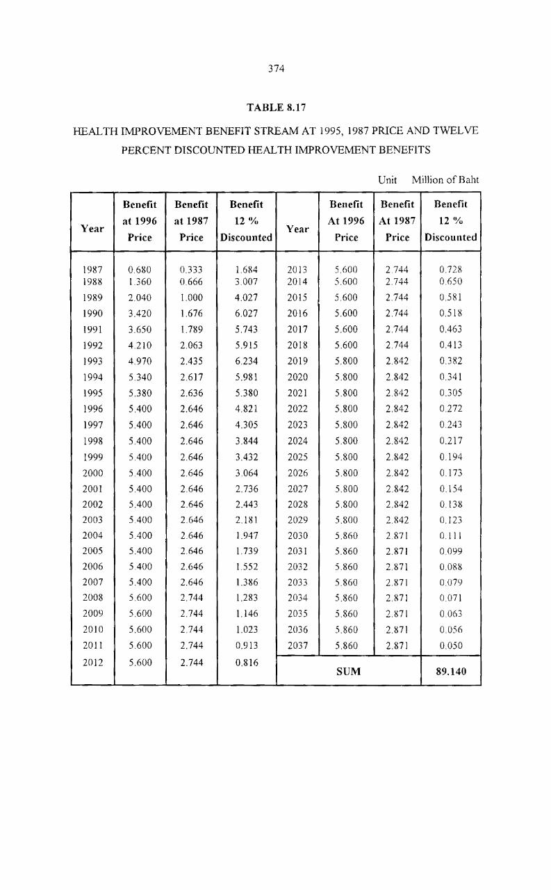
374

TABLE 8.17

HEALTH IMPROVEMENT BENEFIT STREAM AT 1995,1987 PRlCE AND TWELVE

PERCENT DISCOUNTED HEALTH IMPROVEMENT BENEFITS

Unit Million of Baht

Benefit Benefit Benefit Benefit Benefit Benefit

at 1996 at 1987 12 (~, At 1996 At 1987 12 'Yo Year Yeal'

Price Price Discounted Price Price Discounted

1987 0.6lW 0.333 1.684 2013 5.600 2.744 0.728 1988 1.360 0.666 3.007 2014 5.600 2.744 0.650

1989 2.040 1.000 4.027 2015 5.600 2.744 0.581

1990 3.420 1.676 6.027 2016 5.600 2.744 0.518

1991 3.650 1.789 5.743 2017 5.600 2.744 0.463

1992 4.210 2.063 5.915 2018 5.600 2.744 0.413

1993 4.970 2.435 6.234 2019 5.800 2.842 0.382

1994 5.340 2.617 5.981 2020 5.800 2.842 0.341

1995 5.380 2.636 5.380 2021 5.800 2.842 0.305

1996 5.400 2.646 4.821 2022 5.800 2.842 0.272

1997 5.400 2.646 4.305 2023 5.800 2.842 0.243

1998 5.400 2.646 3.844 2024 5.800 2.842 0.217

1999 5.400 2.646 3.432 2025 5.800 2.842 0.194

2000 5.400 2.646 3.064 2026 5.800 2.842 0.173

2001 5.400 2.646 2.736 2027 5.800 2.842 0.154

2002 5.400 2.646 2.443 2028 5.800 2.842 0.138

2003 5.400 2.646 2.181 2029 5.800 2.842 0.123

2004 5.400 2.646 1.947 2030 5.860 2.871 0.111

2005 5.400 2646 1.739 2031 5.860 2.871 0.099

2006 5.400 2.646 1.552 2032 5.860 2.871 0.088

2007 5.400 2.646 1.386 2033 5.860 2.871 0.079

2008 5.600 2.744 1.283 2034 5.860 2.871 0.071

2009 5.600 2.744 1.146 2035 5.860 2.871 0.063

2010 5.600 2.744 1.023 2036 5.860 VPI 0.050

20ll 5.600 2.744 0.913 2037 5.860 2.871 0.050

2012 5.600 2.744 0.816 SUM 89.140

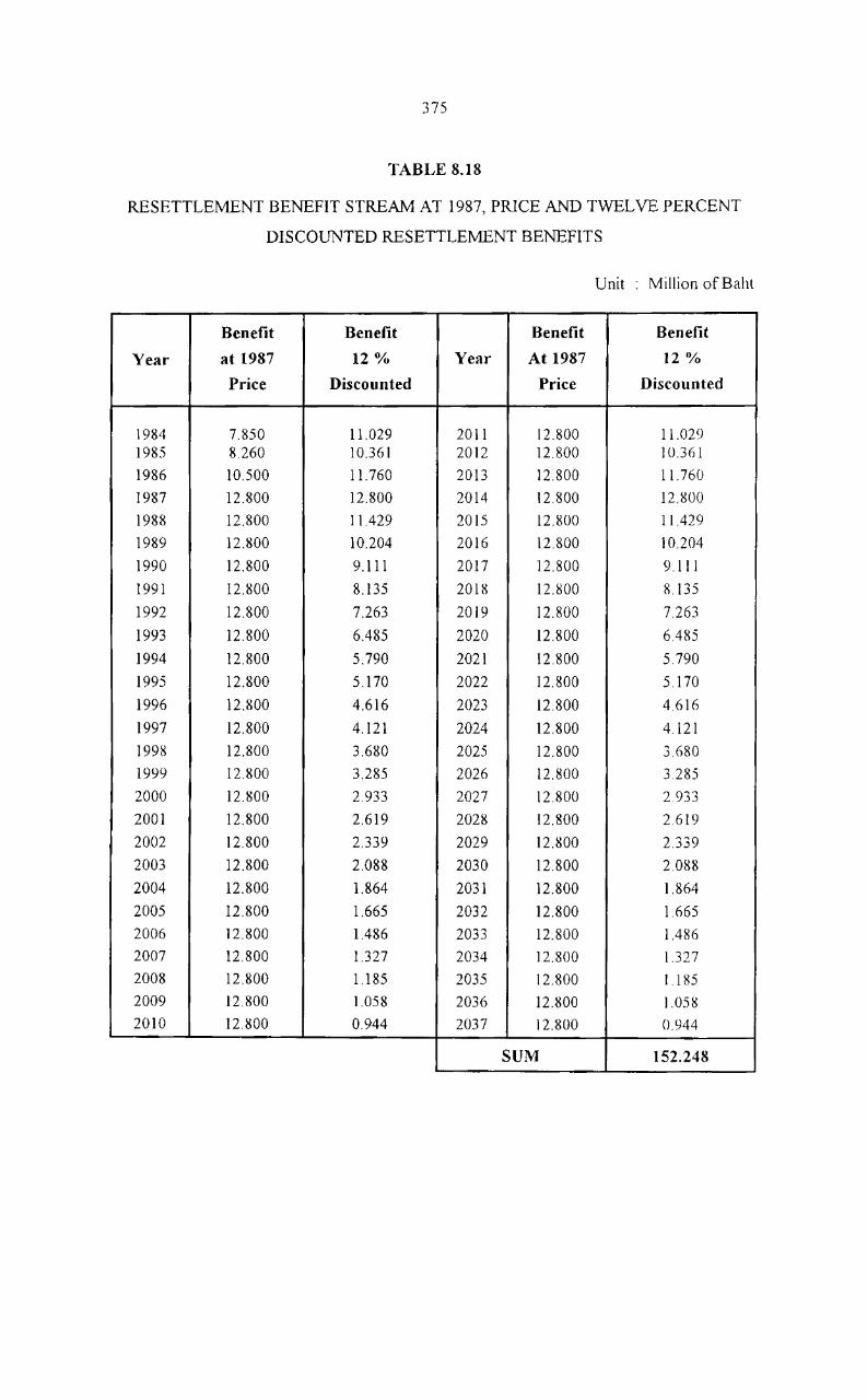
375

TABLE 8.18

RESETTLEMENT BENEFIT STREAM AT 1987, PRICE AND TWELVE PERCENT

DISCOUNTED RESETTLEMENT BENEFITS

Unit Million of Bahl

Benefit Benefit Benefit Benefit

Year at 1987 12 % Year At 1987 12 'Yo

Price Discounted Price Discounted

1984 7.850 1l.029 2011 12.800 11.029 1985 8.260 10.361 2012 12.800 10.361

1986 10.500 11. 760 2013 ]2.800 11.760

1987 12.800 12.800 2014 12.800 12);00

1988 12.800 1 1.429 2015 12.800 11.429

1989 12.800 10.204 2016 12.800 10.204

1990 12.800 9.111 2017 12.800 9.111

1991 12.800 8.135 2018 12.800 8.135

1992 12.800 7.263 2019 12.800 7.263

1993 12.800 6.485 2020 12.800 6.485

1994 12.800 5.790 2021 12.800 5.790

1995 12.800 5.170 2022 12.800 5.170

1996 12.800 4.616 2023 12.800 4.616

1997 12.800 4.121 2024 12.800 4.121

1998 12.800 3.680 2025 12.800 3.680

1999 12.800 3.285 2026 12.800 3.285

2000 12.800 2.933 2027 12.800 2.933

2001 12.800 2.619 2028 12.800 2.619

2002 12.800 2.339 2029 IVWO 2.339

2003 12.800 2.088 2030 12.800 2.088

2004 12.800 1.864 2031 12.800 1.864

2005 12.800 1.665 2032 12.800 1.665

2006 12.800 1.486 2033 12.800 1.486

2007 12.800 1.327 2034 12.800 1.327

2008 12.800 1.185 2035 12.800 1.185

2009 12.800 1.058 2036 12.800 1.058

2010 12.800 0.944 2037 12.800 0.944

SUM 152.248

376

2.4.3 Comparison of Benefits Estimated before and after Project Implementation

In this section the benefits of various components estimated in section 2.4.2

are compared with those estimated before project implementation. Table 8.19 show

benefits estimated before and after project implementation. Benefits from water supply,

salinity and water pollution control, health improvement, and health improvement was not

estimated in monetary value before project implementation.

The present worth of hydropower benefits estimated before project

implementation was 1,853.68 million bahts, while the one estimated after project

implementation is 1650.10 million bahts. This difference is due to the computation of

benefit is based on different sources of power generation. The benefit estimated before

project implementation was based on 80 MW oil-fired plant plus 40 gas turbine plant,

which was the most competitive alternative source of electricity equivalent characteristics

during that period (EEl Report) while the benefit estimated after project implementation is

based on 240 MW gas-fired plant, which is presently the least cost equivalent system.

Moreover, due to oil crisis the cost of fuel for power generation during the period before

project implementation was very high. But during this post evaluation study the oil crisis is

over, and the cost of fuel particularly the cost of gas planed to be used for the 240 MW

gas-fired plant is rather inexpensive sine it can be produced domestically. Therefore, the

present worth of hydropower benefits estimated before project implementation was much

higher than the one estimated after project implementation.

The present worth of irrigation benefits estimated before and after project

implementation are 1,562.48 and 1,482.78 million bahts, respectively.

377

The present worth of flood protection benefits was not estimated before project

implementation. It was only indicated that the benefit would be 23.57 million bahts per

year. From Table 8.9 flood protection benefits estimated after project implementation is

about 216.55 million bahts, higher than the previously estimated one.

The present worth of fisheries development benefits was also not estimated

before project implementation. However, it was estimated that the benefit would be about

27.0 million bahts per year as compared to the average of about 300.76 million bahts

estimated after project implementation.

Again, the present worth of transportation benefits was not estimated before

project implementation. It was only revealed that the road relocation cost was estimated to

be 120 million bahts and the benefit from transportation was about -266.08 million bahts.

The estimation made after project implementation indicated that the cost of road relocation

was about 70.8 million bahts and the benefit from transportation was about -147.73

million bahts per year.

The present worth of forestry benefits estimated before and after project

implementation is about 324.4 and -370.65 million bahts, respectively. The difference,

which is relatively small, is due to the different discount rates adopted in the two

estimations. It was 10 percent in the previous estimation while it is 12 percent in this

updated estimation.

Tourism benefits estimated before project implementation gave the present

worth of about 206.26 million bahts as compared to approximately 176.75 million bahts

estimated after project implementation.

378

TABLE 8.19

COMPARISON OF BENEFITS ESTIMATED BEFORE AND AFTER PROJECT

IMPLEMENTATION (1987 PRICE)

Estimated benefit, Million bahts

Items of benefit Before project After pl'oject

(1) Implementation Implementation

(2) (3)

1. Hydropower 1,853.68 1,650.10

2. Irrigation 1562.48 1,482.78

3. Water supply not estimated 131.2]

4. Flood protection 23.57year 216.25

5. Fisheries development 27.0/year 300.76

6. Transportation and -16/year, and -266.08 -] 47.73

navigation for road relocation

7. Salinity and water pollution

control not estimated negligible 8. Forestry 324.4 -370.65 9. Tourism 206.26 176.75 10 Health improvement not estimated 89.19 11. Resettlement 154.50 152.25

All benefits, except those of items 4, 5 and 6 in column 2, are in terms of

present worth.

379

2.4.4 Project Assessment

Based on Table 8-19, the overall benefit of the project is lower than it was

previously estimated. However, this should not result in the conclusion that the overall

benefit from the project is lower. This was due to external factors. These factors are, for

example, the costs of fuel used in the power generation as already described in section

2.4.3 of this chapter. The less expensive cost of natural gas, which can be produced locally

makes the cost of alternative source of electricity lower. Hence the benefit of the

hydropower generation declines.

Another factor that causes a component of the benefits to be delayed is right­

of-way problem. The right-of-way problem makes irrigation component progresses slO\ver

than it was anticipated. Thus, its benefit during the overall project life is smaller than it was

previously estimated.

Besides, some of the actual benefits derived from the project are greater while

some others are smaller than those previously estimated. However, these differences seem

to be rather insignificant. Therefore, it can be concluded that the overall actual positive

benefit of the project is lower than it was anticipated, and it is caused by external factors.

2.5 Conclusion and Recommendation

The study with regard to demand for electricity of industrial and service units

reveals that the cost of electricity ranges from 8 to 833 bahts per hour. Factor share of

electricity varies from only 1 percent for food canning industry to 82 percent for ice

making factory. Damage due to electricity interruption is estimated to be in the range of 15

bahts per hour for hair dressing service to 3,079 bahts per hour for ice making business.

380

The present worth of benefits, at 1987 and 12 percent discount rate, of

hydropower production, irrigation, water supply, flood protection, fisheries development,

transportation and navigation, forestry, tourism, health improvement, and resettlement are

made. They are approximately 1650.10, 1482.78, 131.21, 300.76, -147.73, -370.65,

176.75,89.14 and 152.25 million bahts, respectively.

Comparison of benefits estimated before and after project implementation has

been made. It is found that the differences in present worth are tremendous for forestry,

hydropower production and irrigation. The ones estimated after project implementation are

about 695, 203 and 79 million bahts, respectively, lower than those estimated before

project implementation. The changes in input and output prices and unexpected delay in

work implementation of irrigation project mainly caused these differences. The differences

between benefits estimated before and after project implementation for forestry and

tourism are rather small. The comparisons of other components of benefits could not be

made directly either because their present worth was not estimated before the project

implementation, or because their benefits were not estimated at all.

381

3. Input-Output Analysis

3.1 Introduction

Like most investment projects, Rajjaprabha dam also produces not only direct

effects, but also indirect effects on output and income in the regional economy

Rajjaprabha dam essentially produces two products: electricity and water. Electricity is

supplied to producing activities, particularly manufacturing as intermediate input, and to

households as consumption goods. Water is distributed mainly for irrigation for

agricultural production. In addition, the construction of the dam also changed the natural

structure of the area. It improves navigation facilities, changes structure of forestry

resources, fisheries resources, etc. Thus, in one way or the another, it affects production

structure of the economy.

The dam affects environment as well. The project Improves flood control

system in the region, reduces salinity damages In the basin, and eliminates or reduces

pollution generated by economic activities, etc. On the other hand, economic expansion

(that generated by the dam) produces by-product as pollution that affects quality of life in

the region

These are direct and indirect effects generated by Rajjaprabha dam should be

included in project evaluation but usually not captured. The purpose of this study is to

analyse direct and indirect effects on output, income and pollution generated by the dam in

the region. Indirect effects are also emphasized.

382

3.2 Objective and Scope

The main objective of this study is to analyse direct and indirect effects of

Rajjaprabha dam on output, income and environment in Surat Thani. So the administrative

boundary of Surat Thani province is defined as a region specific economic system.

Production sectors within the area are "domestic" production sectors and those outside the

area are aggregated as "the rest of the world". Inflows of goods and services from the rest

of the world are considered as "imports" while outflows of goods and services from the

region, "exports".

3.3 Methodology

(1) Model: In addition to the usual input-output matrix, household income

consumption matrices and pollution row are included in the model. The model is described

in details in section methodology chapter 1.

(2) Data: The 1975 national input-output transaction table is used as a basis to

derive regional technical coefficient matrix. Based on economic profIle of the region,

important production activities are identified. Production activities are aggregated into 36

sectors. Households are differentiated between agricultural and non-agricultural

households. The adapted transaction table is used to derive technical coefficient matrix for

the regional economy (Table 8.20). Technical coefficients for households (income and

consumption) are derived from the social account matrix for Thailand. Primary data from

survey, spot check and secondary data from various sources are used to cross check the

technical coefficient matrix. Certain cells have been adjusted. Observation in the area

suggested that air pollution is not important here. Hence, only water pollution is

383

emphasized. As suggested from water quality study, only few industries have more

potential to be pollutant generators. Their pollution coefficients are obtained from water

quality study. Each row represents supply of goods and services from a row sector to

various column sectors while each column represents demand for goods and selvices from

various row sectors. Row households refer to value added to households while column

households refer to consumption of households.

The technical coefficient in Table 8.20, reading along the column, represent the

production function of a column production sector. For example, the value of 0.0318557 of

row 1 column 1 indicates that to produce a unit of paddy, the paddy production sector

(column) requires 0.0318557 units of output from paddy sector itself (row) as input.

Similarly, the value of 0.004224 means that to produce one unit of paddy, the paddy sector

needs 0.004224 units of output from forestry sector as input in the same manner. The value

of 0.858128 in row 37, column I shows that to produce one unit of paddy, the sector

requires 0.858128 units of value added agricultural households. Column 26 of Table 8.20

hence shows the inputs (as outputs from various rows sectors) required for electricity

production. As can be seen, only marginal proportion of inputs from the regional economy

issued in the production process. More than 60% of inputs is supplied from outside the

region (imports).

384

TABLE 8.20

TECHNICAL COEFFICIENTS FOR REGIONAL ECONOMY

-Item 1 2 3 4 5 6 7 -Paddy 1 0.0318557 0 0.0012471 0 0.0066329 0.0281027 0

Beans and Nuts 2 0 0.0124866 0.0007008 0 0 0 0

Vegatable and Fruit 3 0 0 0.0326292 0 0 0.0072246 0 -Rubber 4 0 0 0 0 0 0 0 -Other Crops 5 0.0254730 0.0524014 0.0105930 0.0136359 0.02223520 0 0.0161915

Livestock 6 0 0 0 0 0 0.0013552 0

Forestries 7 0.0004224 0 0.0009008 0 0.0157243 0.0012462 0.0392260

Fisheries 8 0 0 0 0 0 0.0128238 0

Mining and Quarrying 9 0 0 0 0 0 0 0

SlaughteIing 10 0 0 0 0 0 0 0

Oil from Crop or Animal 11 0 0 0 0 0 0 0

Other processing of food 12 0 0 0 0 0 0 0

Rice Mill 13 0 0 0 0 0 0.0658043 0

Ice 14 0 0 0 0 0 0 0

Othe." food 15 0 0 0 0 0 0 0

Animal feed 16 0 0 0 0 0 0.2646912 0

Softdt"ink and Carbonate wat 17 0 0 0 0 0 0 0

Printing and Publishing 18 0 0 0 0 0 0.0000236 0.0000005

Ruhber Sheel and Blacl{ 19 0 0 0 0 0 0 o '

ConCl"ete and Cement Produc 20 0 0 0 0 0 0 0.0036250

Others 21 0 0 0 0 0 0 0.0016081

Motor Vehicle and ReIlail" 22 0,0012898 0.0006722 0.0015695 0.0006838 0.0019193 0.0009403 0.0007747

Saw mill 23 0.0000954 0 0 0 0.0003651 0.0000&07 0

Wood product 24 0.0007049 0.0031391 0.0063901 0.0005778 0.0074544 (LOO03249 0.0012633

Othcl" Manufacturing Goods 25 0 0 0 0 0 0.0000598 0.0000217

Electricity 26 0 0 0 0 0 0.0007761 0

Watcr work and SUl1lllies 27 0 0 0 0 0 0.0022058 0

Building Constmction 28 0.0008743 0.0018651 0.0007805 0.0015234 0.001527 0.0073584 0.0036286

Public wo.-l, and construction 29 0 0 0 0 0 0 0

T."adc 30 0.0095992 0.0056619 0.0196759 0.0074052 0.0141387 0.0542165 0.0064295

Restaurant and Hotel 31 0 0 0 0 0 0 {J

Road tnmspOIiation 32 0.0012135 0.0013258 0.0040037 0.0013791 0.0019729 0.0085740 0.0013l.<6g

\Yater tnmS)IOliation 33 0.0005163 0.0003366 0.0013718 0.0003799 0.0007711 0.0038053 0.0003726

Air tranSllol1ation 34 0 0 0.0000039 0 0.0000177 0.0000033 0

Post and other communic.ttio 35 0 0 0 0 0 0 0

Services 36 0.0191152 0.0072192 0.0075901 0.0049575 0.0016195 0.0090666 0.0027%5

Agdcultural household 37 0.8581280 0.3513223 0.8533162 0.9252000 0.8669900 0.4745680 0.8276400

Nonagdcultural household 38 0 0 0 0 0 0 0

ImJlOl"ts 39 0.0517225 0.0235709 0.0583223 0.0442573 0.5862600 0.5684970 0.332971(0

Pollution 41J 0 0 0 0 0 0 0

Sum raw 1 1 1 1 1 1 1

385

TABLE 8.20 (CONT'D)

Item 22 23 24 25

Paddy 1 0 0 0 0.0132154

Beans and Nuts 2 0 0 0 0

Vegatable and Fruit 3 0 0 0 0

Rubber 4 0 0 0 0

Other Crops S 0 0 0.0000053 0.0001106

Livestock 6 0 0 0 0.0211245

Forestries 7 0 0.4551523 0.0828155 0.0110157

Fisheries 8 0 0 0 0

Mining and Quarrying 9 0 0 0 0

Slaughtering 10 0 0 0 0

Oil from Crop or Animal 11 0 0 0 0

Other processing of food 12 0 0 0 0

Rice Mill 13 0 0 0 0

Ice 14 0 0 0 0

Other food IS 0 0 0 0

Animal feed 16 0 0 0 0

Softdrink and Carbonate wat 17 0 0 0 0

Printing and Publishing 18 0.0003659 0 0 0.0003133

Rubber Sheei and Black 19 0 0 0 0

Concrete and Cement Produc 20 0 0 0 0

Others 21 0 0 0 0

Motor Vehicle and Repair 22 0 0.0118776 0.0073021 0.0011096

Saw mill 23 0 0 0.2055461 0.0308814

Wood product 24 0 0 0.0016607 00043684

Other Manufacturing Goods 25 0.0000307 0.0001035 0.0000925 0.0007684

Electricity 26 0.0055782 0.0182010 0.0127534 0.0055456

Water work and supplies 27 0 0.0004569 0.0005872 0.0001508

Building Construction 28 0.0010512 00033436 0.0062330 0.0033171

Public work and construction 29 0.0001892 0 0.0011613 0.0011258

Trade 30 0.7667880 0.3784480 0.1028118 0.8941570

Restaurant and Hotel 31 0 0.0030870 0.0057141 0

Road transportation 32 0.0129337 0.0184167 0.0145858 0.0083438

Water transportation 33 0.0025053 0.0021706 0.0049356 0

Air transportation 34 0.0000741 0 0 0.0000005

Post and other communicatio 35 0.0005282 0.0008082 0.0024230 0.0001214

Services 36 0.0011654 0.0118434 0.0091193 0.0040038

Agricultural household 37 0 0 0 0

Non-agricultural household 38 0.2771530 0.4093380 0.4047850 0.5448830

Imports 39 0.6217463 0.0273565 0.1374673 0.2601804

Pollution 40 0 0 0 0

Sum Raw 1 I 1 1

26 27

0 0

0 0

0 0

0 0

0 0

0 0

0 0

0 0

0 0

0 0

0 0

0 0

0 0

0 0

0 0

0 0

0 0

0.0005150 0.0002402

0 0

0 0

0 0

0.0014464 0.0006763

0 0

0.0005078 0.0002371

0.0000847 0.0000400

0.0236003 0.1550101

0.0014464 0.0023687

0.0026033 0.0063072

0.0003328 0.0015066

0.0787164 0.0257336

0 0

0.0148873 0.0040617

0.0028161 0.0007933

0.0010324 0.000732

0.0007231 0.0006657

0.0221406 0.0072525

0 0

0.3853920 0.5954770

0.4637553 0.1998979

0 0

I I

28

0

0

0

0

0.0000477

0

0.0083317 ;

o ~ 0 .

0

o. 0

0

0

0

Or

0' ,

0.0001150

0

0

0.0069997

0.0018334

0.7832610

0.0029519

0.0000114

0.0042419

0.0001105

0.0003667

0

0.0874981

0.0063252

0.003509

0.0187963 ,

0.0000001

0.0005788

0.0178769

0.0169430 .

0.3561440

0.3890923

0

1 ,

o

o

o

o O.

O.

o.

O.

o O.

o.

o o o.

o.

0 ..

o.

0 ..

0.·

386

3.4 Analysis Results

The results of the study are presented in two parts. One is the analysis of

structural linkages in the regional economy. The other is the analysis of impacts generated

in the economy by the Rajjaprabha dam.

3.4.1 Structural Linkages

One of the advantages of input-output analysis is that it provides a full picture

of inter-industry relationship in the economy, i.e. direct and indirect relationship. Table

8.21 shows direct and indirect effects on various row sectors that are generated by an

exogenous change in final demand (including household demand), while Table 8.22 shows

the effects generated by other final demand (excluding household demand). Table 8.23

summarizes total effects on production from Table 8.21 and Table 8.22. In addition, total

effects on imports, pollution, and income generated by other final demand are also

presented.

Thus, 1.093124 of fisheries sector means that a unit increase of fisheries final

demand generates 1.6808 units of output in the economy. The distribution of these 1.6808

units are distributed can be seen in fisheries column of Table 8.2!. The same interpretation

is applied to others. As can be seen, figures along column 1 (paddy sector) of Table 8.21

shows output (directly and indirectly) demanded from various row sectors due to unit

increase in final demand for output of the paddy sector. Each element of the diagonal

matrices in Tables 8.21 and Table 8.22 has a value of I for the exogenous final demand

added, while other elements of the matrices refer to direct and indirect demand generated.

For instance, the value of 0.000046 ofrow 6 column 1 in Table 8.21 means that the amount

387

of 0.000046 units of output from livestock are indirectly generated due to an increase in

one unit of final demand for output of paddy sector. It should be noted that this amount is

not directly demanded in paddy production (see the respective cell in table 8.20). Similarly,

along column 26 of Table 8.21, all row sectors have received direct and/or indirect demand

from a unit increase in final demand for electricity. Thus, a unit of final demands for

electricity indirectly generates 0.000078 units of output from paddy sector, and so on.

Total effects from Table 8.21 are conventional input-output inverse, which

have been argued to be inappropriate particularly for rural economy. It has been assessed

that direct and indirect effects are generated not only through production linkages, but also

through income consumption linkages. Through income-consumption linkages, the

increased income (generated due to increase production) must be either spent or saved

depending on behaviours of the resource owners. In Surat Thani province, where more

than 70 percent of household are engaged in agriculture, income-consumption effects

cannot be neglected. The analysis here concentrates on the income-consumption effects.

As shown in Table 8.22, much higher direct and indirect effects are generated in the

economy when income-consumption effects are included. Without income-consumption

effects, a unit increase in final demand for paddy production generates 1. 10 15 units of total

output in the regional economy (the last row of column 1 in Table 8.21). With such effects,

the total outputs of 3.3618 unit are generated. Similarly, an increase in other demand of

electricity generated 2.21347 units of total output compared to 1. I 7685 units of the case

without income consumption effects.

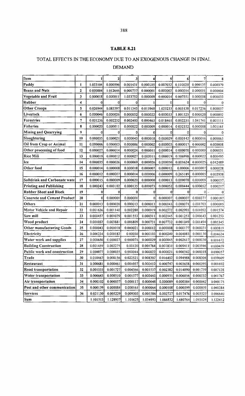
388

TABLES.21

TOTAL EFFECTS IN THE ECONOMY DUE TO AN EXOGENOUS CHANGE IN FINAL

DEMAND

- - -Item I 2 3 4 5 6 7 8

Paddy I 1.033104 0.000596 0.001431 0.000105 0.007032 0.110020 0.000135 . 0.000379

Beans and Nuts 2 0.000004 1.012646 0.000737 0.000001 0.000002 0.000014 0.000001 0.000004

Vegetable and Fruit 3 0.000018 0.000011 1.033752 0.000009 0.000014 0.007551 0.000008 0000033

Rubber 4 0 0 0 1 0 0 0: 0

Other Croops 5 0.026944 0.085397 0.011345 0.013960 1.023233 0.003138 0.017256 0.000037

Livestock 6 0.000046 0.000026 0.000052 0.000022 0.000033 1.001525 0.000020 0.000092

Forestries 7 0.001236 0.002252 0.002400 0.000463 0.018461 0.002231 1.041741 0.001111

Fisheries 8 0.000020 0.000011 0.000022 0.000009 0.000014 0.032352 0.000008 1.001161

Mining and Quarrying 9 0 0 0 0 0 0 0 0

Slaughtering 10 0.000035 0.000021 0.000043 0.000018 0.000029 0.000142 0.000016 0.000065

Oil from Crop or Animal 11 0.000006 0.000003 0.000006 0.000002 0.000003 0.000017 0.000002 0.000008

Other processing of food 12 0.000027 0.000014 0.000024 0.000011 0.000014 0.000070 0.000009 0.000031

Rice Mill 13 0.000019 0.000012 0.000027 0.000011 0.000019 0.106998 0.000022 0.000495

Ice 14 0.000035 0.000026 0.000069 0.000026 0.000050 0.001624 0.000025 0.042489 !

Other food 15 0.000014 0.000008 0.000018 0.000007 0.000012 0.00006 0.000007 i 0.000028

16 0.000012 0.000007 0.000014 0.000006 0.000009 0.265189 0.000005 : 00029381

Softdrink and Carbonate wate 17 0.000015 0.000009 0.000020 0.000008 0.000013 0.000078 0.000009 0.000037

Printing and Publishing 18 0.000243 0.000102 0.000135 0.000073 0.000052 0.000444 0.000052 0000217

Rubber Sheet and Block 19 0 0 0 0 0 0 0 0,

Concrete and Cement Product 20 0 0.000001 0.000001 0 0.000007 0.000007 0.000377 00001871 i

Others 21 0.000013 0.000020 0.000013 0.000013 0.000043 0.000071 0.001703 0.000005]

Motor Vehicle and Repair 22 0.001636 0.001140 0.002280 0.000919 0.0023'72 0.002993 0.001092 0.001574

Saw mill 23 0.000457 0.001029 0.001553 0.000311 0.002145 0.001253 0.000643 0.001253

Wood product 24 0.001032 0.003881 0.006809 0.000731 0.007732 0.001049 0.001494 0.005345

Other manufacturing Goods 25 0.000043 0.OQOOI8 0.000021 0.000012 0.000008 0.000177 0.000031 : 0.000819

Electricity 26 0.000234 0.000182 0.00030 0.000103 0.000249 0.004083 0.000130 6.004624

Water work and supplies 27 0.000650 0.000037 0.000071 0.000029 0.000045 0.002617 0.000030 0.001672

Building Construction 28 0.001459 0.002275 0.00120 0.001784 0.001831 0.009411 0.003946 0.000459

Public work and construction 29 0.000077 0.000035 0.000044 0.000022 0.000021 0.000342 0.000018 0.000057

Trade 30 0.010467 0.008156 0.022521 0.008302 0.016402 0.094988 0.008004 0.039609

Restaurant 31 0.000681 0.000461 0.001057 0.000412 0.000747 0.003658 0.000395 0.001692

Road transportation 32 0.001555 0.001727 0.004566 0.001537 0.002382 0.014090 0.001739 0.007128

Water transportation 33 0.000643 0.000510 0.001577 0.000460 0.000935 0.006056 0.000532 0.001767

Air transportation 34 0.000102 0.000057 0.000117 0.000048 0.000089 0.000384 0.000042: 0.000175

Post and other communication 35 0.000139 0.000084 0.000161 0.000064 0.000108 0.000599 0.000059' 0.000284

Services 36 0.021130 0.005229 0.009303 0.005586 0.002727 0.017476 0.003525, 0.006640

Sum 1.101513 1.128957 1.101625 1.034993 1.086832 1.680764 1.093124: 1.122412

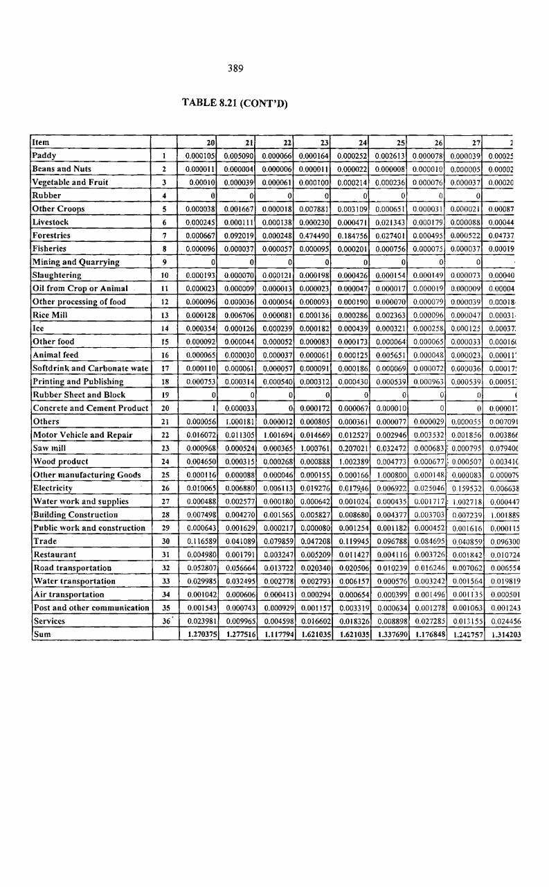
389

TABLE 8.21 (CONT'D)

Item 20 21 22 23 24 25 26 27 2

Paddy 1 0.000105 0.005090 0.000066 0.000164 0.000252 0.002613 0.000078 0.000039 0.0002:!

Beans and Nuts 2 0.000011 0.000004 0.000006 0.000011 0.000022 0.000008 0.000010 0.000005 0.00002

Vegetable and Fruit 3 0.00010 0.000039 0.000061 0.000100 0.000214 0.000236 0.000076 0.000037 0.00020

Rubber 4 0 0 0 0 0 0 0 0

Other Croops 5 0.000038 0.001667 0.000018 0.007881 0.003109 0.000651 0.000031 0.000021 0.00087

Livestock 6 0.000245 0.000111 0.000138 0.000230 0.000471 0.021343 0.000179 0.000088 0.00044

Forestries 7 0.000667 0.092019 0.000248 0.474490 0.184756 0.027401 0.000495 0.000522 0.04737

Fisheries 8 0.000096 0.000037 0.000057 0.000095 0.000201 0.000756 0.000075 0.000037 0.00019

Mining and Quarrying 9 0 0 0 0 0 0 0 0 ,

Slaughtering 10 0.000193 0.000070 0.000121 0.000198 0.000426 0.000154 0.000149 0.000073 0.00040

Oil from Crop or Animal 11 0.000023 0.000009 0.000013 0.000023 0.000047 0.000017 0.000019 0.000009 0.00004

Other processing of food 12 0.000096 0.000036 0.000054 0.000093 0.000190 0.000070 0.000079 0.000039 0.00018,

Rice Mill 13 0.000128 0.006706 0.000081 0.000136 0.000286 0.002363 0.000096 0.000047 000031,

Ice 14 0.000354 0.000126 0.000239 0.000182 0,000439 0.000321 0.000258 0.000125 0.00037:

Other food 15 0.000092 0.000044 0.000052 0.000083 0.000173 0.000064 0.000065 0.000033 0.00016(

Animal feed 16 0.000065 0.000030 0,000037 0.000061 0.000125 0.005651 0.000048 0.000023 0.00011'

Softdrink and Carbonate wate 17 0.000110 0.000061 0.000057 0.000091 0.000186 0.000069 0.000072 0.000036 0.00017~

Printing and Publishing 18 0.000753 0.000314 0.000540 0.000312 0.000430 0.000539 0.000963 0.000539 0.00051:

Rubber Sheet and Block 19 0 0 0 0 0 0 0 0 (

Concrete and Cement Product 20 I 0.000033 0 0.000172 0.000067 0.0000\0 0 0 0.00001~

Others 21 0.000056 1.000181 0.000012 0.000805 0.000361 0.000077 0.000029 0.000055 0.007091

Motor Vehicle and Repair 22 0.016072 0.011305 1.001694 0.014669 0.012527 0.002946 0.003532 0.001856 0.00386f

Saw mill 23 0.000968 0.000524 0.000365 1.000761 0.207021 0.032472 0.000683 0.000795 0.07940~

Wood product 24 0.004650 0.000315 0.000268 0.000888 1.002389 0.004773 0.000677 0.000507 0.00341C

Other manufacturing Goods 25 0.000116 0.000088 0.000046 0.000155 0.000166 1.000800 0.000148 . 0.000083 0.00007S

Electricity 26 0.010065 0.006880 0.006113 0.019276 0.0179;t6 0.006922 0.025046 0.159532 0.00663~

Water work and supplies 27 0.000488 0.002577 0.000180 0.000642 0.001024 0.000435 0.001717 : 1.002718 0.000447

Building Construction 28 0.007498 0.004270 0.001565 0.005827 0.008680 0.004377 0.003703 0.007239 1.001889

Public work and construction 29 0.000643 0.001629 0.000217 0.000080 0.001254 0.001182 0.000452 0.001616 0.000115

Trade 30 0.1\6589 0.041089 0.079859 0.047208 0.119945 0.096788 0.084695 0.040859 0.096300

Restaurant 31 0.004980 0.001791 0.003247 0.005209 0.011427 0.004116 0.003726 0.001S42 0.010724

Road transportation 32 0.052807 0.056664 0.013722 0.020340 0.020506 0.010239 0.0\6246 0.007062 0.006554

Water transportation 33 0.029985 0.032495 0.002778 0.002793 0.006157 0.000576 0.003242 0.001564 0.019819

Air transportation 34 0.001042 0.000606 0.000413 0.000294 0.000654 0.000399 0.001496 0.001135 0.000501

Post and other communication 35 0.001543 0.000743 0.000929 0.001157 0.003319 0.000634 0.001278 0.001063 0.001243

Services 36 0.023981 0.009965 0.004598 0.016602 0.018326 0.008898 0.027285 0.OnI55 0.024456

Sum 1.270375 1.277516 1.117794 1.621035 1.621035 1.337690 1.176848 1.242757 1.314203

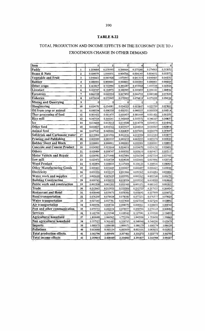
390

TABLEB.22

TOTAL PRODUCTION AND INCOME EFFECTS IN THE ECONOMY DUE TO j

EXOGENOUS CHANGE IN OTHER DEMAND

Item 1 2 3 4 5 (;

Paddy 1 1.203084 0.279393 0.266664 0.275280 0.274903 0.313052

Beans & Nuts 2 0.004079 1.016851 0.004766 0.004145 0.004052 0.003.372

Vegetable and Fruit 3 0.040661 0.041928 1.073947 0.041315 0.040405 0.041232

Rubber 4 0.000001 0.000001 0.000001 0.000001 0.000001 0.000001

Other CI"OPS 5 0.462017 0.533996 0.441687 0.455968 1.455548 0.365324

Lirestact (; 0.101747 0.104973 0.100595 0.103455 0.101121 1.084936

Forestries 7 0.066558 0.069534 0.067452 0.066733 0.083340 0.057633

Fisheries ·8 0.073694 0.075945 0.072912 0.074818 0.073209 0.094124

Mining and Quarrying 9 0 0 0 0 0 0

Slaughtering 10 0.024176 0.024381 0.024223 0.023847 0.023799 0.027891

Oil from crop or animal 11 0.000334 0.000339 0.000331 0.000333 0.000328 0.000314

Thc.- Ill'ocessin~ offood 12 0.001452 0.001475 0.001437 0.001449 0.001426 0.001359

Rice mill 13 0.347524 0.360241 0.342669 0.355572 0.346107 0.368657

lee 14 0.014608 0.015012 0.014508 0.014778 0.014515 0.014342

Other food 15 0.033827 0.034762 0.033527 0.034214 0.033565 0.029&14

Animal feed 16 0.027145 0.028006 0.026839 0.027601 0.026979 0.287447

Softdrink and Cllrbon:lte water 17 0.012261 0.012594 0.012156 0.0[2394 0.012164 0.010877

PI"inting and Publishing 18 0.003389 0.003335 0.003253 0.003255 0.003174 0.003220

Rubber Shcet and Blocl~ 19 o.aooao[ a.OOOOO[ 0.000001 0.000001 0.000001 0.00000 [

Concrete llnd Cement Product 20 0.024305 a.025044 0.024051 0.024670 0.024150 0.020491

Othel's 21 0.009484 0.008747 0.008395 0.009610 0.009457 0.007215

Motor Vehicle and Rcpair 22 0.026981 0.271440 0.027406 0.026534 0.0275 [4 0.025560

Saw mill 23 0.023473 0.024739 0.024330 0.023666 0.025006 0.020714

Wood Product 24 0.102894 0.108835 0.107604 0.104120 0.108916 0.086905

OthCl" Manufactudng Goods 25 0.000463 0.000449 0.000437 0.000437 0.000425 0.000544

Elcctricih' 26 0.031296 0.032135 0.031066 0.03[563 0.031084 0031006

Watcl' wad, and sUl!Jllics 27 0.003600 0.003639 0.003591 0.003565 0.003540 0.006170

Building Construction 28 0.018745 0.020052 0.018324 0.0192[5 0.018988 0.004466

Public work :md construction 29 0.001208 0.00[201 0.001163 0.001 [71 0.001145 0.001205

T'-:Ide 30 0.212842 0.2[ 5923 0.223206 0.212723 0.2[7125 0.266424

Restaurant and Hotel 31 0.058440 0.059673 0.058381 0.058642 0.057999 0.056672

Road tran~0l1ation 32 0.076290 0.078624 0.078580 0.07725 I 0.076577 0.078629

Watel" transpOl-tation 33 0.027145 0.027781 0.027820 0.027314 0.027246 0.028E92

Air transpol1ation 34 0,008596 0.008726 0.008570 0.008561 0.008493 0.008740

Post and other communication 35 0.079753 0.082054 0.078977 0.090792 0.079169 0.068584

Services 36 0.141726 O. [31946 0.128941 0.127281 0.122300 O. [26899

Agl"icultural houschold 37 1.800688 1.866965 1.775290 1.842990 1.793490 1.350849

Non agricultUl'al household 38 0.557327 0.561483 0.558713 0.548948 0.548396 0653479

Imj)OI-ts 39 1.000173 1.000180 1.00017[ 1.000 [79 1.000174 1.000128

Pollutions 40 0.003080 0.003154 0.003059 0.003101 0.003052 0.002922

Tot:" production effects. 41 3.361796 3.459491 3.337411 3.331272 3.322775 3.562792

Total income effects 42 2.3590]5 2.428449 2.334003 2.391837 2.34J9SS 2.004327

391

TABLE 8.22 (CONT'D)

Item 20 21 22 23 24 25

Paddy 1 0.053803 0.086655 0.036039 0.173927 0.112759 0.079111 0.050,

Bcans & Nuts 2 0.001736 0.001587 0.001167 0.003457 0.002809 0.002298 O.OOH

Vegetable and Fruit 3 0.017915 0.026455 0.012051 0.035020 0.028744 0.023929 0.016~

Rubber 4 0.000001 0.000001 0 0.000001 0.000001 0.000001 0.0000

Other crops 5 0.196017 0.226484 0.131935 0.386404 0.314783 0.259740 01841

Lirestact 6 0.042030 0.042676 0.028254 0.095109 0.068542 0.076925 0.0394

Forestries 7 0.038387 0.128694 0.022281 0.534270 0.235468 0.070378 0.0312

Fisheries 8 0.034701 0.039260 0.023354 0.065462 0.054664 0.046384 0.0325'

Mining and Quarrying 9 0 0 0 0 0 0

Slaughtering 10 0.035715 0.035460 0.024094 0.043252 0.047014 0.045030 0.0335'

Oil from crop or animal 1I 0.000249 0.000250 0.000166 0.000378 0.000375 0.000310 0.0002:

Ther processing of food 12 0.001071 0.001078 0.000711 0.001631 0.001607 0001331 0.00095

Rice mill t3 0.067674 0.102541 0.045321 0.222862 0.143464 0.099189 0.0633!

Ice 14 0.005806 0.009383 0.005934 0.014550 0.031220 0.011336 0.08204

Other food 15 0.020493 0.022257 0.013798 0.034127 0,030541 0.026598 0.01924

Animal feed 16 0.011226 0.012999 0.007547 0.022718 0.018301 0.020496 0.01053

Softdrink and Carbonate water 17 0.007576 0.009177 0.005087 0.012489 0.011276 0.009774 000709

Printing and Publishing 18 0.002676 0.002403 0.001835 0.003501 0.003285 0.003037 0.00277

Rubber Sheet and Block 19 0.000001 0.000001 0.000001 0.000001 0.000001 0.000001 0.00000

Concrete and Cement Product 20 1.011758 0.013291 0.007917 0.022040 0.018441 0.015486 0.011051

Others 21 0.004168 1.004915 0.002781 0.008440 0.006782 0.005489 0.00389:

Motor Vehicle and Repair 22 0.032215 0.028749 1.012573 0.040949 0.036302 0.023889 0.01871(

Saw mill 23 0.012306 0.013268 0.007999 1.021653 0.224662 0.047378 0.011331

Wood Product 24 0.049759 0.055894 0.033457 0.092561 1.079413 0.069652 0.047201

Other ManufacturiJ!g Goods 25 0.000362 0.000356 0.000212 0.000571 0.000534 1.001121 0.00038C

Electricity 26 0.027489 0.026058 0.017850 0.049370 0.044276 0.029666 1.041423

Water work and supplies 27 0.004048 0.006229 0.002581 0.005484 0.005895 0.004976 0.00506U

Buildin~ Construction 28 0.017424 0.015135 0.008252 0.022779 0.023605 0.017318 0.013037

Public work and construction 29 0.001156 0.002212 0.005630 0.001068 0.002069 0.001860 0.000934

Trade 30 0.249501 0.184110 0.169431 0.260631 0.314545 0.268969 0.209662

Restaurant and Hotel 31 0.048881 0.046307 0.031492 0.069676 0.071681 0.058166 0.043127

Road transportation 32 0.093957 0.102036 0.041439 0.092058 0.008294 0.064005 0.054925

Water transportation 33 0.044430 0.048452 0.012498 0.029088 0.028105 0.019443 0.016806

Air transportation 34 0.009006 0.008833 0.005785 0.011386 0.011658 0.010587 0.0099881

Post and other communication 35 0.042909 0.046728 0.029787 0.005347 0.066893 0.054855 0.040156

,Services 36 0.102368 0.099110 0.060915 0.147543 0.139286 0.116705 0104713

,Agricultural household 37 0.333881 0.481566 0.223525 1.139695 0.722745 0.481774 0.312762

[Non agricultural household 38 0.861455 0.855585 0.581419 1.030971 1.124742 1.087222 0.810641

'Imports 39 1.000030 1.000014 1.000019 1.000109 \.000064 0.986819 1.000024

Pollutions 40 0.002397 0.002525 0.001616 0.003583 0.003406 0.003084 0002254

Total production effects. 41 2.289821 2.441197 1.804007 3.599692 3.243943 2.585312 2.134721

Total income effects 42 1.195336 1.237152 0.804944 2.170656 1.847487 1.568996 1.123402

392

TABLE 8.23

TOT AL EFFECTS GENERATED ON PRODUCTION, IMPORT POLLUTION AND

INCOME IN THE ECONOMY, WITH AND WITHOUT

INCOME-CONSUM.PTION LINKAGES

Q)

e = o 0 c...I -- ~ = ..... Q) ._ Q. bll

..... ... ~

With income-consumption linkages =.::c: :I ~ = Sectors 0

.:::: c:~ ..... 0

~ C.I

Production Production Imports Pollution Income

1. Paddy 1.1015 3.3618 1.0002 0.0031 2.3380

2. Beans and nut 1.1291 3.4595 1.0002 0.0031 2.4281

3. Vegetable and fruit 1.1017 3.3374 1.0002 0.0031 2.3341

4. Rubber 1.0351 3 .. 3313 1.0002 0.0031 2.3910

5. Other crops 1.0868 3.3328 1.0001 0.0030 2.3410

6. Livestock 1.6808 3.5628 1.0002 0.0029 2.0043

7. Forestry 1.0831 3.3849 1.0001 0.0031 2.3977

8. Fisheries 1.1224 3.1660 1.0001 0.0024 2.1461

9. Mining and quarrying 1.0873 2.7828 1.0001 0.0038 l. 9681

10. Slaughtering 2.3794 4.2322 1.0001 0.0032 2.0186

1 I. Oil from crop/animal 1.4863 3.0497 1.0001 0.0030 1.7432

12. Other processing of food 1.5117 3.1882 1.0002 0.0034 1.8743

13. Rice mill 1.8667 4.0717 1.0000 0.003 I 2.3084

14. Ice 1.183 1 2.7399 1.0000 0.0037 1.8272

15. Other food 1.2533 2.3030 1.0001 0.0024 1.2259

16. Animal feed l.5041 2.7794 1.0000 0.0027 1.4297

17. Soft drink, carbonate water 1.2591 2.5086 1.0000 0.0029 1.4657

18. Printing and publishing 1.2159 2.2047 1.0001 0.0023 1.1593

393

TABLE 8.23 (CONT'D)

~

is c: = = c,) .... '" c: - ~ .. Q. elJ - is ~ With income-consumption linkages = = ..!I::

= '" .S Sectors .c: = -."': =

~ f..I

Pro- Pro-duction duction Imports Pollution Income

1 9. Rubber sheet and block 1.698 3.6674 1.0000 0.0037 2.1309

20. Concrete and cement

product 1.2704 2.2898 1.0000 0.0024 l. 1958

21. Other 1.2775 2.4415 1.0000 0.0025 1.3371

22. Motor vehicle and repair 1.1178 1.8040 1.0001 0.0016 0.8049

23. Saw mill 1.6210 3.5887 1.0001 0.0036 2.1706

24. Wood product 1.6231 2.2438 0.9868 0.0034 1.8475

25. Manufacturing product 1.2377 2.5853 1.0000 0.0031 1.5690

26. Electricity 1.1768 2.1347 1.0000 0.0022 1.1234

27. Water work and supplies 1.2428 2.5937 1.0000 0.0032 1.5853

28. Building construction 1.3142 2.4464 1.0000 0.0025 1.3087

29. Public work/construction 1.2320 2.1940 1.0000 0.0022 1. 125 I

30. Trade 1.1483 2.9009 1.0000 0.0041 2.0500

3 1. Restaurant and hotel 1.4344 2.9318 1.0000 0.0033 1.7259

32. Road transportation 1.2480 2.3976 1.0000 0.0027 1.3465

33. Water transportation 1.1135 1.6033 1.0000 0.0035 1.7454

34. Air transportation 1.1805 2.4187 1.0000 0.0029 1.4524

35. Post and other

communication 1.3218 2.9322 1.0000 0.0038 1.8894

36. Service 1. 1742 2.9109 1.0000 0.0040 2.0214

394

As shown in Table 8.23, with income-consumption effects, agriculture

generates relatively larger multiplier effects than non-agriculture. This is because higher

value added per unit output in agriculture as well as higher marginal propensity for the

consumption of farm households. Most indirect effects are absorbed by paddy, other crops,

rice mill and trade sectors (Table 8.22). Among non-agriculture, agriculture based

industries also produce larger multiplier effects than nonagricuitural-based industries and

services. This implies that an investment that increases output in agriculture or agricultural

based industries produces larger benefits to the economy as a whole. Hence, a multi­

purpose dam like Rajjaprabha dam with improved agriculture in the region has potential to

produce more benefit to the society.

The two products from Rajjaprabha dam, viz., electricity and water, are quite

different in nature. While electricity is a sufficient condition in production structure,

irrigation water is close to necessary condition. Electricity, a service to the economy,

produces relatively small multiplier effects of 2.13. It is not possible to value irrigation

water from the dam directly. From paddy producing sector, it is observed that a much

larger multiplier effects of3.362 are induced.

Production sectors in the economy tend to produce similar effects on imports

and pollution. Regardless of direct structural linkages (Table 8.21), sectors in the economy

eventually induce certain amount of pollution to the system (Table 8.23). Similar to

production effects, high income is directly and indirectly generated by agriculture or

agriculture based industries. Lower income is generated by non-agricuiture-based

industries or services (Table 8.23).

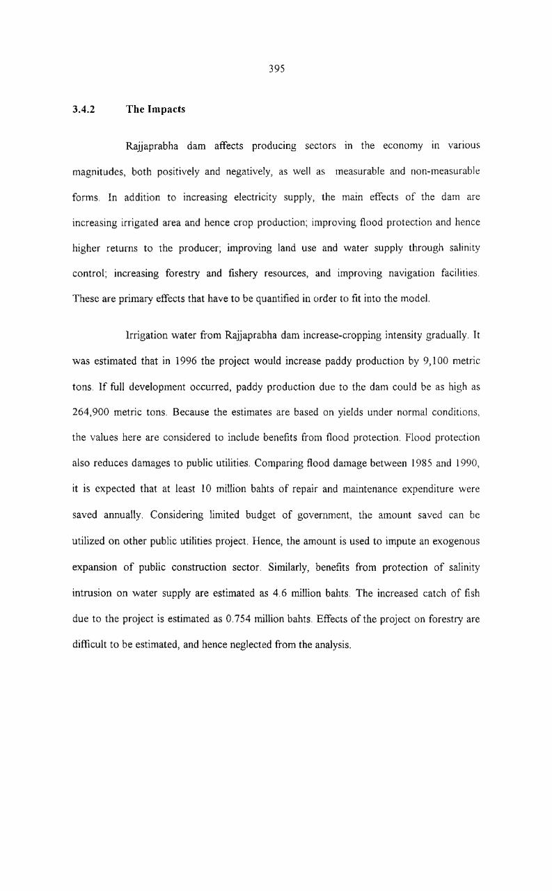
395

3.4.2 The Impacts

Rajjaprabha dam affects producing sectors in the economy in varIOUS

magnitudes, both positively and negatively, as well as measurable and non-measurable

forms. In addition to increasing electricity supply, the main effects of the dam are

increasing irrigated area and hence crop production; improving flood protection and hence

higher returns to the producer; improving land use and water supply through salinity

control; increasing forestry and fishery resources, and improving navigation facilities.

These are primary effects that have to be quantified in order to fit into the model.

Irrigation water from Rajjaprabha dam increase-cropping intensity gradually. It

was estimated that in 1996 the project would increase paddy production by 9,100 metric

tons. If full development occurred, paddy production due to the dam could be as high as

264,900 metric tons. Because the estimates are based on yields under normal conditions,

the values here are considered to include benefits from flood protection. Flood protection

also reduces damages to public utilities. Comparing flood damage between 1985 and 1990,

it is expected that at least 10 million bahts of repair and maintenance expenditure were

saved annually. Considering limited budget of government, the amount saved can be

utilized on other public utilities project. Hence, the amount is used to impute an exogenous

expansion of public construction sector. Similarly, benefits from protection of salinity

intrusion on water supply are estimated as 4.6 million bahts. The increased catch of fish

due to the project is estimated as 0.754 million bahts. Effects of the project on forestry are

difficult to be estimated, and hence neglected from the analysis.

396

Table 8.24 shows total impacts of Rajjaprabha dam on output and income

generated in Surat Thani provinces under present irrigation capacity. Direct benefit of the

dam of less than 45 million bahts generates additional 61.5 million bahts, or about 1.4

times of output in the economy. Benefits to agriculture constitute only about one-third of

total benefits. The remaining benefits are shared between manufacturing and services.

Agricultural households (44 million bahts) mostly capture income generated in

the economy. Non-agricultural households receive about 38% of total income (27 million

bahts). Increase in output and income in the economy also generates additional imports.

About one-third of output is imported. Pollution generated in the economy is 108,000 kg of

BOD equivalent.

Table 8.25 shows output and income generated by the dam with full

development of the irrigation project. Given about 30 times higher output of paddy, the

dam generates more than 20 times of output than the first case. The total output generated

is 1,296 million bahts. Agriculture receives about 37% of total output. of the 1,547 million

bahts of income generated in the economy, agricultural households receive about 73

percent. The remainder is distributed to nonagricultural households. Hence, the larger the

irrigation effects, the higher is the share of total income directed toward agricultural

households than nonagricultural households. Similarly, higher income generates higher

imports (6.90 million bahts). It should be noted that high irrigation benefit also generates

high share of imports to total output. It generates more than 50 percent of output in the

economy. As indicated in Table 8.25, pollution generated in the economy is 2,095 million

kg of BOD equivalent, almost 20 times higher than in the first case.

397

In general, increased irrigated area is likely to contribute more benefits to the

agricultural sector compared to non-agricultural sector. It also tends to generate higher

share to agricultural households than non-agricultural households do. The only drawback

of such increase is that it is also likely to generate larger share of imports to total output.

Considering Surat Thani as a part of the national economy, imports to Surat Thani are

supplied from other regions of the economy as well as from over-seas. Effects on balance

of payments depend on composition of such imports.

No

1

2

3

4

5

6

7

8

9

10

11

12

13

]4

15

16

17

18

19

20

398

TABLE 8.24

DIRECT AND INDIRECT IMP ACT ON OUTPUT AND INCOME

OF EXISTING BENEFIT

Sector Value No Sector Value

Paddy* 27.300 21 Other 0.514

Beans and nut 14.719 22 Motor vehicle and repair 3.001

Vegetable and fruit 2.098 23 Saw mill 0.013

Rubber 1.408 24 Wood product 1.622

Other crops 2.164 25 Manufacturing product O. [28

Livestock 0.000 26 Electricity 0.573

Forestry* 1.353 27 Water work and supplies * 4.600

Fisheries 0.751 28 Building construction 0.032

Mining and quarrying 0.010 29 Public work and

Slaughtering 0.040 construction* 10.000

Oil from crop/animal 8.264 30 Trade 7.953

Other processing of 31 Restaurant and hotel 2.053

food 0.403 32 Road transportation 2.915

Rice mill 1.076 33 Water transportation 1.176

Ice 0.002 34. Air transportation 0.332

Other food 0.358 35 Post and communication 4.441

Animal feed 0.118 36 Services 4.782

Soft drink, carbonate 37 Agricultural household 44.031

water 0.002 38 Non agricultural 27.461

Printing and publishing 0.722 Household 27.461

Rubber sheet and block 0.264 39 Imports 38.041

Concrete and cement 40 Pollution 0.109

product 1.026

* Notes denotes sectors primarily affected

399

TABLE 8.25

DIRECT AND INDIRECT IMP ACT ON OUTPUT AND INCOME OF FULL BENEFIT

No Sector Value No Sector Value

1 Paddy* 794.700 21 Other 4.588

2 Beans and nut 334.949 22 Motor vehicle and repair 66.187

3 Vegetable and fruit 53.447 23 Saw mill 0.243

4 Rubber 27.731 24 Wood product J 8.869

5 Other crops 47.552 25 Manufacturing product J .941

6 Livestock 0.000 26 Electricity J 1. 150

7 Forestry* 23.205 27 Water work and supplies * 4.600

8 Fisheries 0.754 28 Building construction 0.486

9 Mining and quarrying 0.189 29 Public work and

10 Slaughtering 0.773 construction* 10.000

1 1 Oil from crop/animal 211.780 30 Trade 150.194

]2 Other processing of food 7.697 31 Restaurant and hotel 39.4100

13 Rice mill 22.417 32 Road transportation 51.743

14 Ice 0.002 33 Water transportation 18.342

15 Other food 7.430 34. Air transportation 5.991

16 Animal feed 2.346 35 Post and communication 52.532

17 Soft drink, carbonate 36 Services 95.350

water 0.033 37 Agricultural household 1130.61

18 Printing and publishing 15.882 38 Non agricultural 4J6.549

19 Rubber sheet and block 5.449 household

20 Concrete and cement 39 Imports 698.687

product 17.684 40 Pollution 2095

'" Note'; denotes sectors primarily affected

CHAPTER IX

CONCLUSION AND RECOMMENDATIONS

CHAPTER IX

CONCLUSION AND RECOMMENDATIONS

1. INTRODUCTION

This post evaluation of environmental consequences of Rajjaprabha dam IS

conducted ten years after its commencement.

The Rajjaprabha dam project was planned and implemented as a mUltipurpose

project, mainly for hydropower production, flood protection, fisheries, recreation and

irrigation. The project includes the dam and reservoir with a 240 MW hydropower plant

located about 90 km upstream from Surat Thani province, and irrigation systems covering

the coastal plain in Surat Thani. The upstream storage reservoir (with about 5,639 mcm

storage) and the hydropower plant had already been implemented. The first phase of

irrigation system covers an area of 23,100 hectares. The second phase is envisaged to cover

about 50,000 hectares. But this has not yet been implemented. When the project was

completed it was expected to provide the following benefits: (1) generation of about 554

GWh power per year from the 240 MW installed capacity plant, (2) irrigation of about

50,000 ha, of land, and (3) flood protection and drainage for the towns of Surat Thani and

other downstream communities including the paddy areas in the coastal plain.

2. OBJECTIVES OF THE STUDY

This study was conducted with the following objectives: (I) to assess all

existing environmental resources and their values with the help of input-output analysis

(2) to findout the beneficial impacts of the project (3) to evaluate the actual positive effects

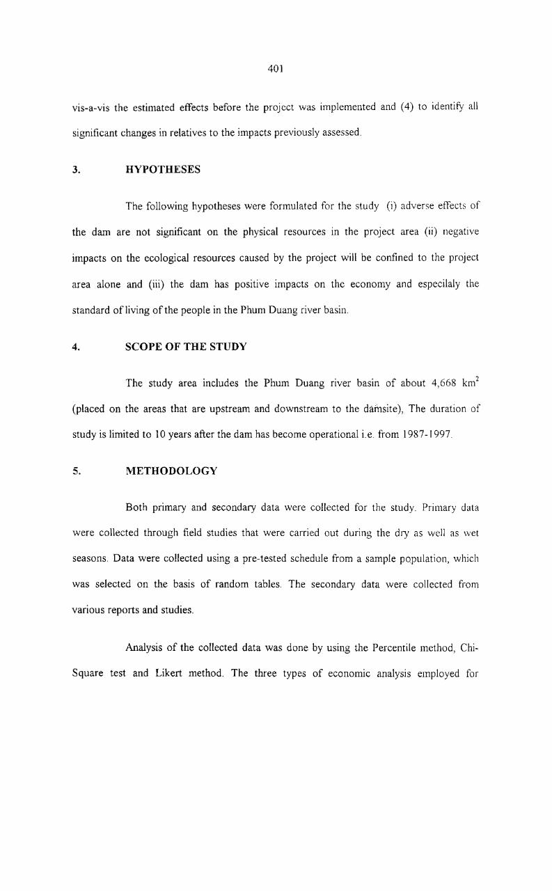
401

vis-a-vis the estimated effects before the project was implemented and (4) to identify all

significant changes in relatives to the impacts previously assessed.

3. HYPOTHESES

The following hypotheses were formulated for the study (i) adverse effects of

the dam are not significant on the physical resources in the project area (ii) negative

impacts on the ecological resources caused by the project will be confined to the project

area alone and (iii) the dam has positive impacts on the economy and especilaly the

standard of living of the people in the Phum Duang river basin.

4. SCOPE OF THE STUDY

The study area includes the Phum Duang river basin of about 4,668 km2

(placed on the areas that are upstream and downstream to the damsite), The duration of

study is limited to 10 years after the dam has become operational i.e. from 1987-1997.

5. METHODOLOGY

Both primary and secondary data were collected for the study. Primary data

were collected through field studies that were carried out during the dry as well as wet

seasons. Data were collected using a pre-tested schedule from a sample po.pulation, which

was selected on the basis of random tables. The secondary data were collected from

various reports and studies.

Analysis of the collected data was done by using the Percentile method, Chi­

Square test and Likert method. The three types of economic analysis employed for

402

valuation of environmental values are: (i) market value (ii) travel cost method and (iii)

survey techniques.

The economIC evaluation of environmental consequence consists of three

aspects: (i) the implication at the regional level (ii) the evaluation of actual positive

benefits at the project level and (iii) input-output analysis to ascertain the etTects of the

project implementation on the regional economy of Surat Thani province.

6. MAJOR FINDINGS OF THE STUDY

The major finding of the study are presented below:

6.1 Physical resources

The results of the study reveal that there is no significant changes in climatic

and ground water resources, with respect to the study area inspte of the fact that the

physical and chemical properties of the soil have slightly changed. Sedimentation in the

reservoir does not have much effect on the function of the dam. But it is seen that water

quality in the reservoir has changed significantly. On the basis of this the first hypothesis is

rejected.

6.2 Ecological resources

No change has occurred in the amount of plankton in the reservoir. But the

composition of fish has changed. Earlier it was the herbivorous variety, which was more in

the catches. But now the carnivorous variety is grown in the dam, which is more beneficial

to fisherman. This is a man made change. Before construction of the dam there was large

scale illegal logging but after completion of the dam, this has come down. But construction

403

of the dam has caused loss of at least 165 km2 of forest area, i.e. submerged under water

Before construction of the dam there were 179 species of animals and other fauna in the

area. Those have been reduced to 152 after construction of the dam. On the basis of this

finding the second hypothesis is rejected.

6.3 Implication on Regional Economics

The main objective of the macroeconomic analysis of the project is to determine

the extent to which the development project is consistent with and contributory to the

achievement of objectives and priorities enunciated in the national development program.

The economic base of the project area is predominantly agriculture. The real

per capita Gross Provincial Product (GPP) of the project area is lower than the average of

the southern region, and also lower than the average of the upper southern region . . " Although the economic base of the project area is under transition i.e. moving away from

agriculture, the area would depend on agriculture for a long time to come. The decline in

importance of agriculture in Surat Thani is due to growth of other sectors. Surat Thani has

a very strong economy. It enjoys higher economic growth in other non-agriculture sectors

and higher investment in construction and public physical infrastructure. Even through the

province used to be confronted with economic fluctuations, it maintained a positive growth

of 5 percent in crops production.

6.4 Actual Positive Benefits

Evaluation of actual positive benefits involves assessmg benefits of varioLls

interrelated multipurpose components of the project. Hence a benefit-cost analysis is done

to evaluate the overall impact.

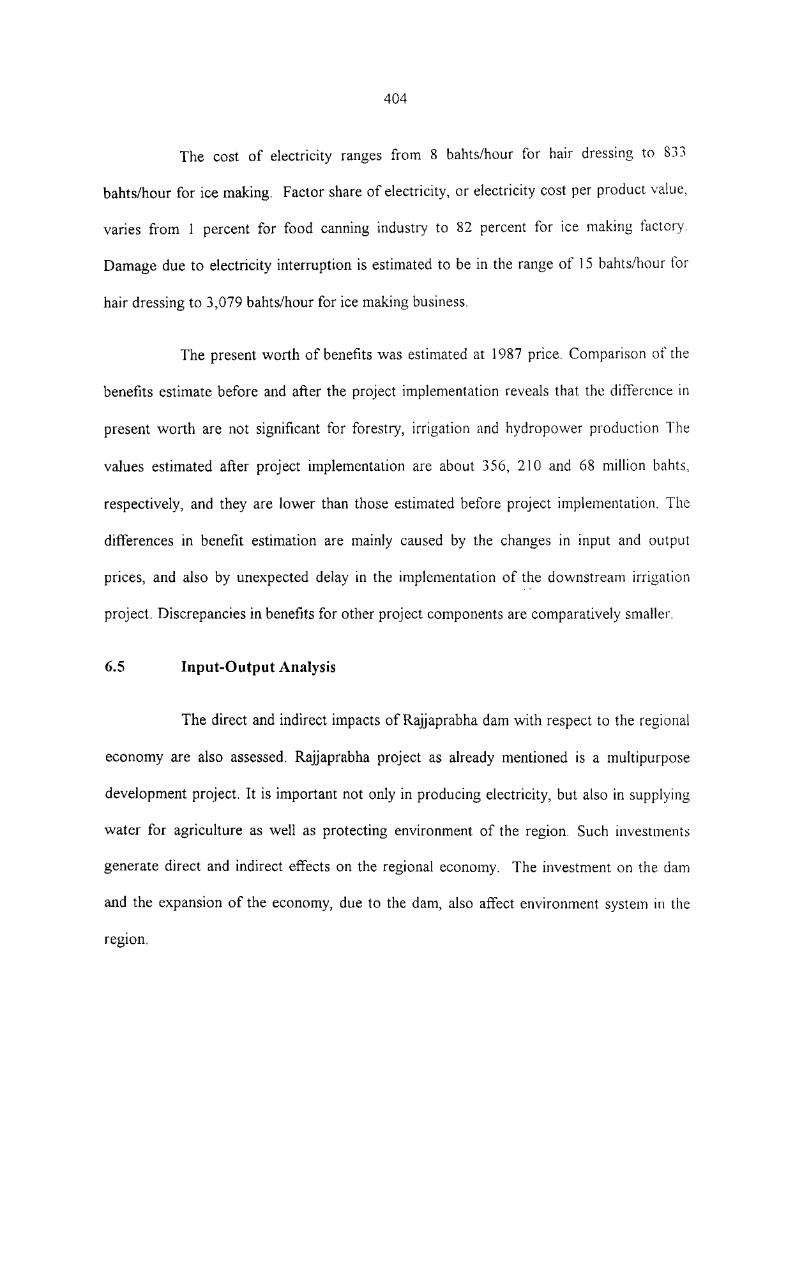
404

The cost of electricity ranges from 8 bahts/hour for hair dressing to 833

bahts/hour for ice making. Factor share of electricity, or electricity cost per product value,

varies from I percent for food canning industry to 82 percent for ice making t~lctOry.

Damage due to electricity interruption is estimated to be in the range of 15 bahts/hour for

hair dressing to 3,079 bahts/hour for ice making business.

The present worth of benefits was estimated at 1987 price. Comparison of the

benefits estimate before and after the project implementation reveals that the difference in

present worth are not signiflcant for forestry, irrigation and hydropower production The

values estimated after project implementation are about 356, 210 and 68 million bahts,

respectively, and they are lower than those estimated before project implementation. The

differences in benefit estimation are mainly caused by the changes in input and output

prices, and also by unexpected delay in the implementation of the downstream irrigation

project. Discrepancies in benefits for other project components are comparatively smaller.

6.5 Input-Output Analysis

The direct and indirect impacts of Rajjaprabha dam with respect to the regional

economy are also assessed. Rajjaprabha project as already mentioned is a multipurpose

development project. It is important not only in producing electricity, but also in supplying

water for agriculture as well as protecting environment of the region. Such investments

generate direct and indirect effects on the regional economy. The investment on the dam

and the expansion of the economy, due to the dam, also affect environment system in the

reglOn.

405

Positive and negative effects of the project are analyzed based on structural

relationships between economic activities and households in the economy. Evaluation of

the total impacts of the project on the regional economy is also emphasized.

By allowing full multiplier effects (i.e., including production and income­

consumption effects), the analysis of structural linkages of economic activities in the

regional economy indicates that agriculture generates larger multiplier effects than non­

agriculture. This is largely because of the higher value added per unit of output in

agriculture than that in non-agriculture, and a higher marginal propensity to consume in the

case of agricultural households than that of non-agricultural households. An increase in

one baht worth of other demand for agricultural products in the economy will generate

more than three bahts of total output in the economy. Similarly, any increase in one baht of

other demand for most non-agricultural products will generate about two bahts worth of

total output in the economy. The increase in one baht of other demand increase household

income ranging from less than one to more than two bahts, imports by about one baht, and

water pollution by 0.0016 to 0.004 kg of BOD. Thus the results show that agriculture is a

more important multiplier effect generator than non-agriculture, on both output and

IHCOIIIC.

Excluding electricity produced, primary effects of the Rajjaprabha dam in the

regional economy are defined as higher paddy and fish production, improvement of flood

protection, and better control of salinity intrusion. Under the existing irrigation capacity, it

is estimated that total indirect effects generated by the dam was about 62 million bahts or

about 1.4 times of its primary effects. Hence, the total effects on output in the economy as

generated by the dam were more than 104 million bahts. Rajjaprapha dam contributed 71

'\

\

406

million bahts to gross regional product, increased 38 million bahts of imports and lO8

thousand kilograms of BOD.

If full development of the irrigation project is realised, the dam will indirectly

generate more than 20 times higher output in the first case. Total output generated is

estimated at 2,016 million bahts. It is likely to contribute about 1,547 million bahts to gross

regional product. Similarly, it is also expected to generate larger imports and intensity

pollution in the region than in the first case.

In sum, the total effects of Rajjaprabha dam on the regional economy are

enormous. The indirect benefits of economic activities from the project vary from sector

to sector, depending on their inter-relationships with the primarily affected sectors. ln

aggregate, agricultural households receive larger shares of benefits than non-agricultural

households. Distribution of benefits, however, depends on the weight of each household

class to the total population. So the third hypothesis is accepted.

From the above findings, the following recommendations are made:

General criteria for watershed management to serve multiple purposes while

sustaining desirable ecological balance should be done as follows.

(1) Land should be used in accordance with its potential, i.e., land of high

agricultural potential should be used for crop production. Other lands ot

low agricultural potential should be assessed for their suitable was such as

agro-forestry or wildlife management.

‘

407

(2) Consideration should be given to prevailing environment in the planning

and development. Local environment should be regarded as an already

functioning ecosystem, and within which agricultural and other land use

development are to take place in harmony with the prevailing environment;

(3) More attention should be paid to etliciency and long term stability of

agricultural and silvicultural systems. They should be regarded as

ecosystems, particularly regarding the resources depletion and environment

deterioration;

(4) Land use planning should consider both increased productivity and soil and

water conservation;

(5) Comprehensive ecosystem analysis, including such aspects as energy flow,

nutrient cycling, population dynamics, and others crucial to successful land

management should be a prerequisite for watershed management; and

(6) Industrial development may create serious adverse impact on renewable

resources. Hence such development should be carefully planned and

located in the watershed with adequate control, and also with properly

planned monitoring program.

\

REFERENCE

REFERENCES

A.H.G. Mitchell, B. Young and W. Jantaranipa, (1970), The Phuket Group,

Peninsular Thailand: A Paleozoic Geosynclines Deposit, Geological Management

Vol. 107, N0. 4, pp. 411-428.

A.T. Ippen and D.R.S Harleman, (1961), One-Dimensional Analysis of Salinity

Intrusion in Estuaries, Committee on Tidal Hydraulics, U.S. Army Corps of

Engineers, Vicksburg, Miss, Tech.bull. No.5, June 1961.

Adkins, W.G. and Burke D., (1974), “Interim Report”: Social Economic and

Environmental Factors in highway Decision Making, Research Report N0.148-4

Austin, Texas: Texas Transportation Institute, Texas A & M University.

Alfred Blumstein, (1971), Cost-Effectiveness Analysis (in Cost-Benefit Analysis),

English University presses Ltd.

Allen V. Kneese, (1977), Economic and Environment, Kingsport Press, lnc,

Kingsport Press, Inc., Kingsport, Tennessee USA.

Anderson L.E (1986), The Economics of Fisheries Management. (Baltimore: The

Johns Hopkins University Press).

Andrews W.H., Madsen, G.E. and Legaz, G.J., (1974), “Social Impact of water

Resource Development and their Implications for Urban and RuralDevelopment”: A Post Audit Analysis off the Weber basin Project in Utah,

Research Monograph No.4. Olga Utah: Institute for Social Science research on

Natural Resources, University of Utah.

Andrews R.N.L., (1973), “Approaches to impact Assessment”: Comparison and

critique paper presented to short course on Impact Assessment in Water resources

Planning, Ann Arbor, Michigan 9 June 1973.

409

APHA, WPCF, (1971), Standard Method for the examination of Water and

Wastewater, American Public Health Association, 13th edition, Washington D.C.

U.S.A.

Architects 110 Ltd. Parts, and Electrowatt Engineering Services Ltd., (1979),

Preliminary Tourism Development Study of Songkhla & Hat Yai, for Tourism

Authority of Thailand.

B. Lekakul and E.W.Gronin, ( 1974), Bird Guide of Thailand, 2”“ Kunispha Ladprao

press, J r, Bangkok, Thailand.

B. Lekakul and J.A. McNeely, (1977), Mammals of Thailand, Kumspha Ladprao

press, Bangkok, Thailand.

B.G. Liptak, (1974), Environmental Engineer’s Handbook, Water Pollution V.1.

Chilton Book Company, Pennsylvania, USA.

B.S. Harris and A.D. Meister, (1987), “A report on use of a Travel Cost Demand

Model for recreation Analysis in New Zealand”: An Evaluation of Lake Tutira,

Discussion paper in Natural Resource Economic No.4 Dept. of Agricultural

Economics and Farm Management, Massery University, Palmeston North, Australia,

No date.

Baker J.K., Dee N. And finally J.R., (1974), Measuring impact of water resource

developments on the human environment, Water Resources Bulletin, 10(1), pp. 10.

Bateman ET. Al. (1992), An Introduction of Estimation of the Benefits of Non­

Priced Recreation Using the Travel-cost Method. Working Paper 36, ESRC

countryside Change Initiative University of Newcastle

Battelle Pacific Northwest Laboratories. (1974), Environmental Assessment

Manual, Columbia River and Tributaries, Northwest Pacific Division, U.S. Corps

of Engineers.

410

Boonchana Klankamsorn and Thongchai Charuppat, (1996), Forest Situation of

Thailand in the past 21 years (during 1974-1995), Forest Management Division,

Royal Forestry Department, Thailand.

Brin D. Clark, Ronald Bisset and Peter Wathern, (1980), Environmental Impact

Assessment, R.K. Bowker Company, New York, USA.

Burchell R.W. and Listokin, D., (1975), The Environmental Impact Handbook,

New Bruswick, New Jersey: center for Urban Policy Research, Rutgers University.

Bureau of Reclamation, (1983), Guide for Computing Degradation, Denver, June

1983.

C. Kanasutara, (1971), On the Fun of Freshwater Clams of Thailand, Ann. Rept.

1971, Inland Fisheries Division, Department of Fisheries, Bangkok, Thailand.

C.J.kreb, (1972), “Ecology” The Experimental Analysis of Distribution and

Abundance Harper & Row publisher, San Francisco USA.

Cater E.C., Hacener L.E. and Hall, J.W., (1972), An Informational Report on

techniques for Evaluating Factors Relevant to Decision-Making on Highway

Location, Washington D.C., Department of Transportation.

Central New York Regional Planning and Development Board, (1972),

Environmental Resources Management, New York: Central New York Regional

Planning and Development Board (PB-217 517), U.S.A.

Chin Yudee, (1974), Mental Drums, In the past, Fine Arts Department, Silpakorn

University, Bangkok, Thailand. Pp. 148-174.

Cicehethi and Freeman, (1971), Option Demand and Consumer Surplus, Further

Comment Quarterly Journal of Economics Vol. 85 No. 3. October 1971.

Clark B.G., Chapman K. Bisset, R and Wathern P., (1978), Methods of

Environmental Impact Analysis, Built Environmental, 4 (2) pp 1 11-121.

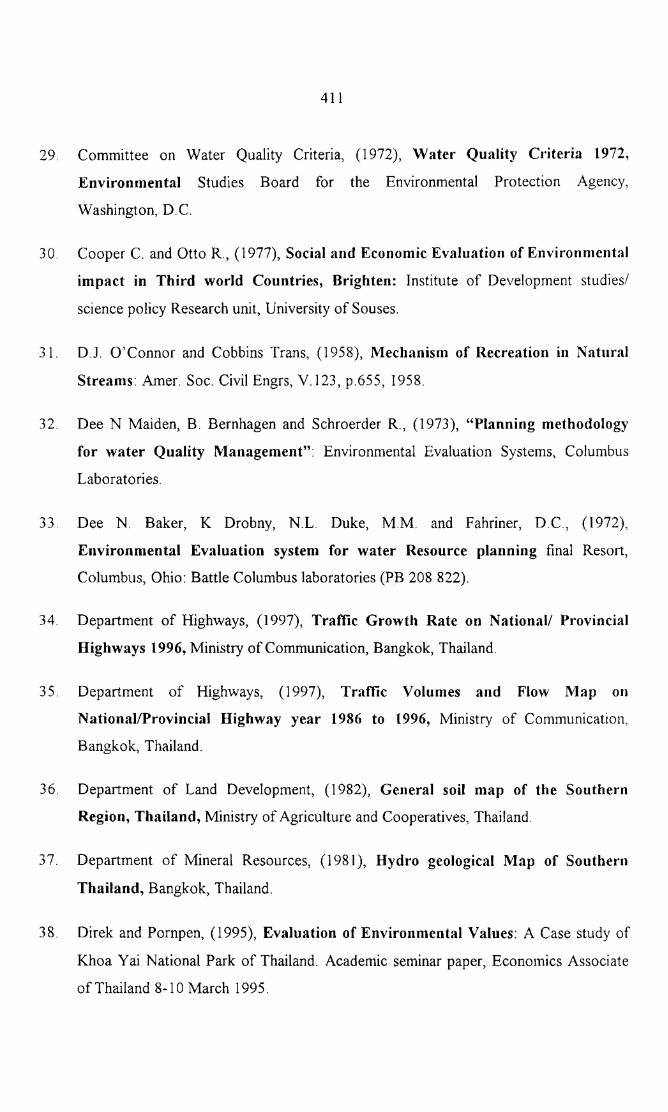
411

Committee on Water Quality Criteria, (1972), Water Quality Criteria 1972,

Environmental Studies Board for the Environmental Protection Agency,

Washington, D.C.

Cooper C. and Otto R., (1977), Social and Economic Evaluation of Environmental

impact in Third world Countries, Brighten: Institute of Development studies/

science policy Research unit, University of Souses.

D.J. O’Connor and Cobbins Trans, (1958), Mechanism of Recreation in Natural

Streams: Amer. Soc. Civil Engrs, \/.123, p.655, 1958.

Dee N Maiden, B. Bernhagen and Schroerder R., (1973), “Planning methodology

for water Quality Management”: Environmental Evaluation Systems, Columbus

Laboratories.

Dee N. Baker, K Drobny, N.L. Duke, M.M. and Fahriner, D.C., (1972),

Environmental Evaluation system for water Resource planning final Resort,

Columbus, Ohio: Battle Columbus laboratories (PB 208 822).

Department of Highways, (1997), Traffic Growth Rate on National/ Provincial

Highways 1996, Ministry of Communication, Bangkok, Thailand.

Department of Highways, (1997), Traffic Volumes and Flow Map onNational/Provincial Highway year 1986 to 1996, Ministry of Communication,

Bangkok, Thailand.

Department of Land Development, (1982), General soil map of the Southern

Region, Thailand, Ministry of Agriculture and Cooperatives, Thailand.

Department of Mineral Resources, (1981), Hydro geological Map of Southern

Thailand, Bangkok, Thailand.

Direk and Pornpen, (1995), Evaluation of Environmental Values: A Case study of

Khoa Yai National Park of Thailand. Academic seminar paper, Economics Associate

of Thailand 8-10 March 1995.

412

Division of Communication Diseases Control, (1995), Annual Report 1995,

Ministry of Public Health, Bangkok, Thailand.

Division of Nutrition, (1997), Normal Weight and Degree of Malnutrition Thai

Children, Age 0-5 years, Department of Health, Ministry Public Health. Bangkok­

Thailand

Eberhardt L.L., (1976), Quantitative ecology and impact assessment, Journal of

Environmental Management, 4 (1) pp. 27-70.

Economics and Information Division, (I984), “Mineral Statistics of Thailand:

1979-1983, Department of Mineral Resources, Thailand.

ELC-Electroconsult Co. Ltd., (I973), Ta Pi - Phum Duang River basinDevelopment, Volume 2: Khlong Saeng project Feasibility study, Royal irrigation

Department, Thailand.

ELC-Electroconsult Co. Ltd., (1973), Ta Pi - Duang River basin Development,

Volume 1: comprehensive study, Royal Irrigation Department, Thailand.

ELC-Electroconsult, C0. Ltd., (I973), Chiew Larn feasibility Report, Volume l:

Main Report, Bangkok Thailand.

Engineering Division, (1975), Preliminary Report on Khlong Maluan Project

Phun Phin district Surat Thani province, Irrigation District Ofiice ll, Royal

Irrigation Department, Approx.1975, in Thai Version.

Engineering Division, (I977), Preliminary Report on Khlong Tha Chang Project,

Tha Chang district, Surat Thai province, Irrigation District ofiice ll, Royal

Irrigation Department, approx. 1977, in Thai Version.

Environment Canada, (1975), Guideline for preparing Initial Environment alEvaluation. Ottawa; Environment and Fisheries Canada.

Environmental Division, (1978), Tender Documents Environmental and

Ecological Investigation of Chiew Larn project, Public Communications Office,

Electricity Generating Authority of Thailand.

413

Environmental Division, (1979), Preliminary Environmental and Ecological

Investigation of Chiew Larn Project, Report No. 154-20-21-29, Public

Communication Ofiice, Electricity Generating Authority of Thailand.

Eversley D.E.C., (1976), Social and economic implication of environmental

impact Assessment, Farnborough Hampshire: Saxon House, pp. 126-41.

F. Loetsch and K.E. Haller, (1964), Forest Inventory, Volume 1, BLV. Verlagsgell­

Schaft Munchen Basel Wien.

Faculty of Agriculture, (1976), Lecture Manual on Economic Crops, Kasetsart

University, Bangkok, Thailand.

FAO., (1979), A Provisional Methodology for Soil Degradation Assessment, FAO.

Fine Arts Department, (1973), Tabien Boran Vattu Tourajanajak 2516, Ministry of

Education. Bangkok, Thailand p. 546 (in Thai version).

Fisheries Economic and Planning sub-division, (1996), Freshwater Fish Farm

Production 1997, Department of Fisheries, NO. 1 1/ 197, Bangkok, Thailand.

G. Bygarrd, (1996), Plankton from Two Lakes of the Malayan Region, Dansk.

Natrukistorisk Foreign Copenhagen.

G.I. Weber, (1971), A Guide to the Common Diatoms at water pollution

surveillance system stations, U.S. Environmental protection Agency, Nat. Envi. Res.

Center, Cincinnati, Ohio.

G.W. Prescott, (1982), Algae of the Western Great Lakes Areas, Wm. Brown

Company Publications.

Ghanshyam N. Singh et al, (1991), Environmental Economics, Cambridge Printing

Works New Delhi, India.

Gilliland M.W. and Risser O.G., (1977), “The Use of systems diagram for

environmental impact assessment”: Procedures and an application Ecological

Modeling, 3(3), pp. 188-209.

414

Ground Water Division, (1996), Ground Water Resources in Southern of

Thailand, Department of Mineral Resources Bangkok, Thailand.

H.B.N. Hynes, (1972), The Ecology of Running Water, University of Toronto press,

USA.

H.S. Swingle, Agric. Exp. Stn. Auburn, (1970), Relationship and Dynamics of

Balanced and Unbalanced Fish Population, Bull. No. 274, 1970

Halvoresen R. and Ruby M.G. (1981), Benefit-Cost Analysis of Air Pollution

Control (Lexington: D.C. Heath and company).

Hartwick J.M. and Olewiler, N.D. (1986), The Economics of Natural Resource Use,

(New York: Harper & Row).

Holling C.S. (ed) (1978), Adaptive Environment Assessment and Management,

Chishester: Wiley.

Howe C.W_ (1979), Natural Resource Economics, (New York: John Wiley &

Sons).

Hunting Technology Services Limited, (1971), South Thailand Regional Planning

Study, Vol. l, for National Economic and Social Development Board, BangkokThailand.

Hupschmidt M.M. et. al. (1983), Environmental Natural Systems andDevelopment An Economic valuation Guide, (Baltimore: The Johns Hopkins

University Press).

Hyde L.W., (1974), Environmental Impact Assessment by Use of Matrix Diag

Montgomery, Alabama Development Office. (PB -235-221).

Hydro Power Construction Department, (1987), Completion Report: Chiew

Multipurpose Project, Electricity Generating Authority of Thailand,

415

Hydrologic Engineering Center, (1966), Generalized Computer Program: Unit

Graph and Hydrographic Computation, U.S. Army Corps ofEngineers, July

Hydrologic Engineering Center, (I987), Hydrograph Combining and Routing, U.S.

Army Corps of Engineers, Computer Program 23-J2-L232.

Hydrology Section, (1986), Sediment Study of Pattani Project, Survey Division,

Planning Department, Electricity Generating Authority of Thailand Report No. HD­

OI0, December 1976.

Hydrology Section, (1987), Records of Wells Drilled by Groundwater Exploration

and Development Project, (October 1985 - September 1986), Volum XIV,

Groundwater Division, Department of Mineral Resources, Thailand.

Hydrology Section, (1996), Report on the Survey of Sedimentation in Ubolratana

Reservoir, Sun/ey Division, Planning Department, Electricity Generating Authority

of Thailand, Report No. 842-2202, in Thai Version, March 1996.

Hydrology Section, (1997), Records of Well Drilled by Groundwater Exploration

and Development Project (October I995-September 1996), Volume XII,

Groundwater Division, Department of Mineral Resources, Thailand.

I. Kurger, (1989), The water supply of Surat Thani, Master plan and Feasibility

Report, for Public Works Department, Surat Thani Provincial.

I.S.R. Munro, (I985), The Marine and Freshwater Fishes of Ceylon, Department

of External Afiairs, Canberra.

ICUN, UNEP and FAO, (I995), National Conservation plan for Thailand (1990~

l994)”, Volume 2 (2nd Draft), Morges, Switzerland.

Institute of Ecology, (1971), Optimum pathway Matrix Analysis Approach to the

Environmental Decision-Making process. Athens, Georgia: University of Georgia

Institute of Ecology.

416

J. Thiemmedth, (1976), Edible Mollusks of Thailand, Faculty of Fisheries,

Kasetsart University, Bangkok, Thailand.

J.C. Waterlow, R. Buzina, W. Keer, J.M. Lane and M.Z. Nichaman, (1977), The

Presentation a Dues of Height and Weight Data for Comparing the Nutritional

Status of Groups of Children Under the Age of 10 Years, WHO Bulletin, Series

No. 55, 1977.

J.C.Waterlw, R.Buzina, W.Keller, J.M. Lane, M.Z. Nichanman and J.M. Tanner,

(1977), The Presentation and use of Height and Weight Data for comparing the

Nutritional Status of Groups of Children under the Age of 10 years, WHO Bulletin,

series No. 55.

J.T. Davis and J.S. Hughes, (1971), Effects of standing Timber on Fish Population

and Fishermen success in Bussey Lake, Louisiana Res. Fish. Lim, AFS. Spec. Pub.

No. 8, Washington, D.C., USA.

Jirasak Jindarojana, et. al., (1979), Nam Pong Environmental Management

Research Project: Working Document No.11, Interim Committee for Coordination

of Investigation of Lower Mekong Basin, Khonkhan, Thailand.

Joskow 1., (1973), Cost benefit analysis for environmental impact statements

public utilities fortnightly, 9 (2).

K. Biswas and C.C. Calder, (1973), Hand Bulletin No.24, Malaria Bureau No.11,

Delhi: Manager of publications, India.

K. Biswas, (1949), Systematic Enumeration of the Most Common Species of

Fresh and Brackish Water Algae, Rec. Bot. Sirv. India.

K. Chunkaew, P. Kurat, S. Boonyawat, P.D hammanonda and N. Panburana, (1976),

Soil and Water losses of Mae Hud Forests in Lampang, Kog-Ma Watershed,

Research Bulletin No. 28, Faculty of Forestry, Kasetsart University, Bangkok,Thailand.

417

K.C. Sankaranarayanan and Karunakaran V., (1984), Tool and Techniques in

Environmental Impact, Cochin University of Science and Technology.

K.C. Sankaranarayanan, (1981), Evaluation of Hydro-Electric Project: “Silent Valley

An economic evaluation of environmental consequences, Indian Manager Vol. Xll N

2 April - June 1981, India.

K. Chunkaew, (1981), Introduction to Watershed Tesources Management in

Humid Tropics, Regional Training Course on Watershed Resources Management

and Environmental Monitoring in Humid and Tropical Ecosystems, May 25 ­

June 8, 1981

K.F. Lagler, (1990), Freshwater Fisheries Biology, WMC Brown Company

Publication, Lowa, USA.

Keeney, R.L. and Raiffa, G.A., (1977), Assessing and evaluating environmental

impacts at proposal nuclear power plant sites, Journal of environmental

management 4 (2), pp. 153-66.

Kula. E. (1992), Economics of Natural Resource and the Environment. (London

Chapman & Hall).

Lamb and Alastair, (1986), The bases of Glass Vessels from Kedha and Takua Pa

Compared in Federation Museum Journal, New series, Vol VI, pp. 56-63.

Lubin S., (1977), Environmental Impact of the Senegal River Basin Project,

KIDMA (Israel journal of Development), 3 (3) pp. 369.

Leontief W. (1970), Environmental Repercussions and the Economics Structure;

and Input-Output Approach. The review of Economics and statistics. 52. No.3 Aug.

260-271.

M. De Backer and K. Openshaw, (1992), Timber Trends Study, Thailand” Detailed

Description of Surveys and Results, FAO No.TA 3156, Rome.

418

M. Watanasak, (1978), A Preliminary Study on the Evaluation of Soil Erosion

Status Using Universal Soil Loss Equation and LANDSAT Image Techniques in

Chonburi and Rayong Provinces” Unpublished M.S. Thesis, Faculty of Graduate

Studies, Mahidol University, Bangkok, Thailand, pp. 38.

M.E. Harr, (1962), Groundwater and Seepage, McGraw Hill Book Company, New

York, USA.

M.M. Hutschimidt et al, (1983), Environment, Natural system and development:

An Economic Valuation Guide, John Hopkins University presses. Baltimore.

M.N. Murty, (1968), Economic Evaluation of Environmental Management

Programmes, Commonwealth Publishers New Delhi, India.

M.S. Garson B. Young, A.H.G. Mitchell and B.A.R. Tait, (1975), The Geology of

the Tin Belt in Peninsular Thailand, Mineral Resource Department, Bangkok.

Malaria Region IV, (Songkhla Province) (1997), Annual Record of Malaria

Region IV, 1995-1996, Ministry of Public Health, Thailand.

Masahiro lmbo, (1974), Sediment Distribution in the Ta Pi Estuary, Thesis No.

646, Asian Institute of Technology, Thailand.

Mc Gauhy P.H., (1968), Engineering Management of Water Quality, McGraw Hill

Book Company.

Mcharc I., (1968), A comprehensive Highway Route Selection Method, Highway

Research Record No. 246 Washington D.C.: Highway Research Board.

Mekong Secretariat (MKG/30), (1975), Pa Mong Downstream Effects on

Hydrology and Agriculture in the Cambodian part of the Mekong Delta Annex

3, (10 pages), for the Mekong Committee, November 1975.

Meteorological Department, (1977), Climatological Data of Thailand - 25 year

Period (1951-1975), Ministry of Communications, Thailand.

419

Ministry of Public Health, (1996), Malaria Annual Report 1996, Bangkok,Thailand.

Marshall C.W., Dee N., Grifiin J. And Goodman, (1973), Development of the

Arizona Environmental and Economic Trade-Off Model. Final Report. Columbia

Ohio: Battelle Columbus Laboratories.

Mizuno Toshihiko and Syuiti Mori, (1970), Preliminary Hydro-biological Survey

of some Southeast Asian Inland Waters Biology, J. Linn. Soc.

Multiagency Task Force, (1972), Guideline for implementing principles and

Standards for Multi objective planning of water resources reviews Draft.

Washington D.C. United State Bureau of Reclamation.

Munn R.E. (ed), (1975), Environmental Impact Assessment Principle and

procedures, SCPOE Reports. Toronto: International Council of Scientific Unions

Scientific Committee on Problems of the Environment.

N. Tangtham, K. Chunkaew and S. Ungkulpakdikul, (1972), Surface Runoff and

Sediment from Natural Forest and Shifting Area on Mountainous Watershed,

Research No.10, Faculty of Forestry, Kasetsart University, Bangkok, Thailand.

Nail K. Shastree, (1991), Evaluating Development Projects. (Environmental

Economics). Mittal publication A-l l0, Mohan Garden New Delhi.

National Economic and Social Development Board, (1998), Economic and Social

Development plan for the Southern Region and Provinces in the Eight Economic

and Social Development Master Plan (in Thai version), Priminister Office,Thailand.

National Environmental Board of Thailand, (1979), Manual of NEB Guideline for

Preparation of Environmental Impact Evaluation, Bangkok, Thailand.

Newman P., (1974), Environment Impact: Part I Development of a semi-quantitative

parameter and its implication Journal of Environmental System 4 (2), pp. 97-102.

123

124

125

126

127

128

I29

130

131

132

133

420

Nichoison W. (1978), Microeconomic Theory: Basic Principles and Extension.

(Illinois: The Dryden Press).

Odum H.T., (1972), Use of Energy Diagram for Environmental Impact

Statements, in Tools of Coastal Management (Proceeding of the conference

February 14-15) Washington D.C. Washington D.C. Marine Technology Society pp.

197-1213.

Ofiice of Accelerated Rural Development (1996), Deep Wells Drilled in the Phum

Duang river basin. Ministry of Interior, Bangkok, Thailand.

Pearce D.W and Turner R.K. (1990), Economic of Natural Resources and the

Environment, (Baltimore: The Johns Hopkins University Press).

P. Prachantha, (1985), Art of the South off Thailand, Muang Boran Journal, V. 5,

No. 2, January-March 1985.

Parker B.C. and Howard R.V., (1977), The first environment monitoring and

assessment in Antarctica: The Dry Valley Drilling Project. BiologicalConservation 12 (2).

Parthum Chumpenpun, (1974), Ancient Remains in the upper part of Southern

Region, Fine Arts Department, Bangkok, Thailand.

Pigou A.C. (1962), The Economics of Welfare. (London: Macmillan & Co. Ltd).

Piriya Krairiksh, (1980), Art in Peninsular Thailand prior to the Fourteenth

Century A.D., Fine Arts Department Bangkok, Thailand.

Planning Department, (1979), Chiew Larn Project Reservoir Simulation-Unit

Installation 4 Units, Electricity Generating Authority of Thailand.

Planning Department, (1979), Dam Height Optimization for Update Feasibility

Study Chiew Laru Project, Electricity Generating Authority of Thailand, Report

No. 841-2202, February 1979.

421

Planning Department, (1987), Summary Report on Ta pi-Phum Duang River

basin Development (in Thai version), Electricity Generating Authority of Thailand.

Project Planning Division, (1990), Irrigation Projects in Southern "River Basins

Draining into the Gulf of Thailand, the West Cost and Indian Ocean, Royal

Irrigation department, in Thai Version.

R. Dudal, (1970), Key to Soil Units for the Soil Map of the World, FAO,UNESCO.

R. Dudal and Goodale T. (Eds.) (1986), Environmental Impact Analysis:

Philosophy and Methods, Madison, Wisconsin University of Wisconsin Sea Grant

Program, pp. 107.

Rapport D.J and Regier H.A., (1977), The application of ecological modeling to

impact assessment inplewes, Toronto: University of Toronto Institute for

Environmental studies pp. 79-97.

Randal. A. (1987), Resource Economics. (New York: John Wiley & Sons).

Rietveld P., (1980), Multiple Objective Decision Methods and Regional Planning

North-Holland, Amsterdam.

Roberts H.A. and Sievsring H., (1976), A preliminary Guide for Benefit

Considerations in Economic Impact Studies Park Forest, South Illinois:

Governors state University (PB-259 169).

Roberts V. Thomann, (1972), System Analysis and Water Quality Management.

MC Graw—Hill New York.

Rosen S. (1974), Hedonic Price and Implicit Makers: Product Differentiation in

Project Competition, Journal of Political Economy, 82, 1:34-35)

Rosen S.J., (1976), Manual for Environmental Impact Evaluation Englewood

Cliffs, New Jersey Prentice-Hall.

422

Ross J.M., (1976), The Numeric Weighting of Environmental Interactions,

Occasional paper No. 10 Ottawa: Lands Directorate Environment Canada.

Royal Irrigation Department, (I975), Ta Pi-Phum Duang River Basin Project, in

Irrigation News letter, Thailand.

S. Piyasin, (1975), Stratigraphy and Sedimentology of the Kaeng Krachan Group

(Carboniferous), Department of Geological Science, Chiengmai University, Spec.

Pub. No. 1 (Proc. Conf. Geol. Thailand, Chiangmai Univ. I973), Vol. 2, pp. 26-36,.

S.A. Schumm, (1969), River Metamorphosis, Hydraulic Division Journal of ASCE,

Volume 95, No. HY 1, January 1969.

Sathit Wacharakitti and others, (I978), The Assessment of Forested Area from

LANDSAT Imagery, a Paper presented at I978 Annual Forestry Conference at

Royal Forest Department, 6-14 November I978.

Schram G., (I973), Accounting for non-economic goals in benefit-Cost analysis,

Journal of Environmental Management 1(2) pp. 129-50.

Sidney Siegel, (1965), Non-parametric Statistics for the Behavioral Science, New

York, McGraw Hill Book Company, pp. 226.

Sinden J.A. and Worrell, A.C. (1979), Unpriced Values: Decision without Market

Price (New York: John Wiley and sons).

Smith M.A., (I974), Field Test of Environment Assessment Methodology:

Environmental Resources center Georgia Institute of Technology, Atlanta Georgia.

(PB-236 045)

Soil and Geology Division, (I977), Report on the Survey of Groundwater

Resources, in Tambon Maluan, Phun Phin district, Surat Thani province, Royal

Irrigation Department, Approx. 1977, in Thai Version.

Soil Survey Division, (1972), National Soil Classification System, Department of

Land Development, Thailand.

156

157

158

159

160

161

162

163

164

165

423

Sondheim M.W., (1978), A comprehensive methodology for assessingenvironmental impact. Journal of environmental Management 6(1) pp. 27-42.

Sorensen J.C. and Pepper J.E., (1972), Procedures for Regional Clearinghouse

review of Environmental Impact Statement, Berkely, California: Association of

Bay Area Governments. (PB-224 57 8).

Southwest Pipe & Supply Co. Ltd., (1982), Preliminary Agricultural Planning and

Identification of the Most Efficient distribution System of the nine Zone Project,

Prepared for the Royal Irrigation Department, Bangkok, Thailand.

Stoloff D., Kammerer R., (1978), Site screening to minimize socio economic

impacts of power facilities, Social Impact Assessment No. 33 pp.217.

Stover L.V., (1972), Environmental Impact Assessment. A procedure Pottstown,

Pennsylvania: Sanders and Thomas.

Surat Thani Provincial Public Health Ofiice, (1996), Annual Report, 1995, Surat

Thani Province, Thailand.

Survey Division, (1979), Hydrological Investigations of Chiew Larn Project,

Planning Department, Electricity Generating Authority of Thailand. Report No. 842

Suzuki Y., Ito K. and Ono T., (1978), A simulation model for regional

environmental impacts analysis-a case study of the Kinki region. International

Journal Environmental studies. 10 (2). Pp. 91-99.

System Planning Division, (1987), Transmission System for Chiew Larn

Hydroelectric Project, Planning Department, Electricity Generating Authority of

Thailand, Report No. 844-2301 revised from Report no. 844-2213.

T. Carstens and Solvik, (1975), Reservoir Erosion, Proceeding of the World

Congress on Water Resources; Water for Human needs, Volume IV Management

and Education, IWRA, New Delhi, India.

424

T. Eren, (1971), The Integrated Watershed Approach for Development Project,

Formulation in FAO - in Guideline for watershed Management FAO conservation

guide No. 1, 1971.

T. Herb, (1964), Freshwater Moleskin Fauna of Thailand, Reprinted from Natural

and Life in Southeast Asia, volume 11 1, Kyoto, Japan.

T.Yamane, (1974), “An lntroductionary Analysis”: Statistics, Harper & Row

Publishers, lnc. 3rd Edition New York 1974.

Team Consulting Engineers Co., Ltd. And others, (1980), Chiew Larn Project

Environmental and Ecological Investigation, Prepared for the Electricity

Generating Authority of Thailand, Bangkok.

Tietenberg T. (1984), Environmental and Natural Resource Economics(Glenview: Scott, Foreman and Company).

Thailand Electric Power Study team, (1966), Thailand Electric Power Study,

United States Operations Mission, for the Royal Thai Government.

Thailand Industrial Standard Institute, (1978), Standards for Industrial Products:

Drinking Water, No. TISI 257, Volume l~1978, Ministry oflndustrial, Thailand.

Toftner R.O., (1973), A Balance Sheet for the Environment Planning 39 (l) pp. 22-25.

Tuntawiroon Nart, (1985) Environmental Science and Resources Administration,

Mahidol University Bangkok Thailand.

U.Yongbunkaid, (1975), Some weeds in paddy Field, Technical paper, Ministry of

Agriculture and cooperatives, Thailand.

United States Department of the Interior, (1974), Design of Small Dams Bureau of

Reclamation, United States Government Prining Ofiice, Washington, USA.

United States Department of Agriculture, (1978), Predicting Rainfall Erosion

Losses: A guide to Conservation Planning, Agricultural Handbook No. 537, USA.

425

USAD. (I989), Soil Taxonomy 1 A Basic System of Soil Classification for making

and Interpreting , Soil Conservation Sen/ice, Agricultural.

V. Champhaka, (1979), Watershed status in Thailand, Watershed Conservation.

Division, Royal Forestry Department, Thailand.

W.W. Massie, Coastal Engineering Group, (1982), Coastal Engineering, Vol. ll,

Department of Civil Engineering, Delft University of Technology.

Warner M.L. and Preston E.H., (1974), Review of Environment Impact Assessment

Methodologies. Washington D.C.: US. Environmental Protection Agency.

Wassily Leontiefi (I970), Environmental Repercussions of the Economic

Structure: An Input-Output Approach, Review of Economic and Statistics, Vol.

III August 1970 pp. 262-71.

Water Allocation and Maintenance Division, (I978), Water Quality for Irrigation,

Irrigation Manual No.15, Royal Irrigation Department, Thailand. (27)

Wells R., (1973), Impact zoning a framework for innovative design in college of

the engineering (ed.) Proceedings, Planning and design for urban runoff and

Sediment Management Lexington, Kentucky: College of Engineering University of

Kentucky pp. I-5.¢

Whitman I.L., Dee N. Mcginnis J.T. Fahringer D.C. and Baker J.K., (I971), Design

of an Environmental Evaluation System. Columbus, Ohio: BattleColumbus

laboratories. (PB -201 743).

Whitney M. Borland, (1973), Pa Mong Phase II-Supplement to Main Report

(Hydraulics and Sediment Studies), Prepared for Mekog Committee, USBR.

VVHO, (I 976), Nutrition in Preventive Medicine”. WHO, V.2, Geneva.

WHO, (1984), Guideline for Drinking Water Quality. WHO, V. 1, Geneva.

426

Wilhelmus A Hafkamp (1984), Economic-Environmental Modeling in a national­

regional system, Elsevier Science Publishers B_V. PO. BOX. 1991 AmsterdamNetherlands.

Wischmeier W.H., C.B. Johnson and B.V. Cross, (1971), A Soil Credibility

Monograph for Farm Land and Construction Site, Journal of soil and water

conservation volume26 (September- October 1971), pp. 189-192.

World Health Organization, (1972), International Standards for Drinking Water,

Geneva, Switzerland,

Yorque R., (1975), Methodologies for Environmental Impact Assessment.

Progress Report No. PR-1 Vancouver: University of British Columbia Institute of

Resource Ecology.