
IJCSI - Semantic Scholar · Mr. Kavi Kumar Khedo, University of Mauritius, Mauritius Dr. B....
66
IJCSI IJCSI International Journal of Computer Science Issues Volume 7, Issue 4, No 3, July 2010 ISSN (Online): 1694-0784 ISSN (Print): 1694-0814 © IJCSI PUBLICATION www.IJCSI.org
Transcript of IJCSI - Semantic Scholar · Mr. Kavi Kumar Khedo, University of Mauritius, Mauritius Dr. B....

IJCSIIJCSI
International Journal of
Computer Science Issues
Volume 7, Issue 4, No 3, July 2010 ISSN (Online): 1694-0784 ISSN (Print): 1694-0814
© IJCSI PUBLICATION www.IJCSI.org

IJCSI proceedings are currently indexed by:
© IJCSI PUBLICATION 2010 www.IJCSI.org

IJCSI Publicity Board 2010 Dr. Borislav D Dimitrov Department of General Practice, Royal College of Surgeons in Ireland Dublin, Ireland Dr. Vishal Goyal Department of Computer Science, Punjabi University Patiala, India Mr. Nehinbe Joshua University of Essex Colchester, Essex, UK Mr. Vassilis Papataxiarhis Department of Informatics and Telecommunications National and Kapodistrian University of Athens, Athens, Greece

EDITORIAL In this fourth edition of 2010, we bring forward issues from various dynamic computer science areas ranging from system performance, computer vision, artificial intelligence, ontologies, software engineering, multimedia, pattern recognition, information retrieval, databases, security and networking among others. Considering the growing interest of academics worldwide to publish in IJCSI, we invite universities and institutions to partner with us to further encourage open-access publications. As always we thank all our reviewers for providing constructive comments on papers sent to them for review. This helps enormously in improving the quality of papers published in this issue. Apart from availability of the full-texts from the journal website, all published papers are deposited in open-access repositories to make access easier and ensure continuous availability of its proceedings. We are pleased to present IJCSI Volume 7, Issue 4, July 2010, split in nine numbers (IJCSI Vol. 7, Issue 4, No. 3). Out of the 179 paper submissions, 57 papers were retained for publication. The acceptance rate for this issue is 31.84%. We wish you a happy reading! IJCSI Editorial Board July 2010 Issue ISSN (Print): 1694-0814 ISSN (Online): 1694-0784 © IJCSI Publications www.IJCSI.org

IJCSI Editorial Board 2010 Dr Tristan Vanrullen Chief Editor LPL, Laboratoire Parole et Langage - CNRS - Aix en Provence, France LABRI, Laboratoire Bordelais de Recherche en Informatique - INRIA - Bordeaux, France LEEE, Laboratoire d'Esthétique et Expérimentations de l'Espace - Université d'Auvergne, France Dr Constantino Malagôn Associate Professor Nebrija University Spain Dr Lamia Fourati Chaari Associate Professor Multimedia and Informatics Higher Institute in SFAX Tunisia Dr Mokhtar Beldjehem Professor Sainte-Anne University Halifax, NS, Canada Dr Pascal Chatonnay Assistant Professor MaÎtre de Conférences Laboratoire d'Informatique de l'Université de Franche-Comté Université de Franche-Comté France Dr Karim Mohammed Rezaul Centre for Applied Internet Research (CAIR) Glyndwr University Wrexham, United Kingdom Dr Yee-Ming Chen Professor Department of Industrial Engineering and Management Yuan Ze University Taiwan

Dr Vishal Goyal Assistant Professor Department of Computer Science Punjabi University Patiala, India Dr Dalbir Singh Faculty of Information Science And Technology National University of Malaysia Malaysia Dr Natarajan Meghanathan Assistant Professor REU Program Director Department of Computer Science Jackson State University Jackson, USA Dr Deepak Laxmi Narasimha Department of Software Engineering, Faculty of Computer Science and Information Technology, University of Malaya, Kuala Lumpur, Malaysia Dr Navneet Agrawal Assistant Professor Department of ECE, College of Technology & Engineering, MPUAT, Udaipur 313001 Rajasthan, India Dr T. V. Prasad Professor Department of Computer Science and Engineering, Lingaya's University Faridabad, Haryana, India Prof N. Jaisankar Assistant Professor School of Computing Sciences, VIT University Vellore, Tamilnadu, India

IJCSI Reviewers Committee 2010 Mr. Markus Schatten, University of Zagreb, Faculty of Organization and Informatics, Croatia Mr. Vassilis Papataxiarhis, Department of Informatics and Telecommunications, National and Kapodistrian University of Athens, Athens, Greece Dr Modestos Stavrakis, University of the Aegean, Greece Dr Fadi KHALIL, LAAS -- CNRS Laboratory, France Dr Dimitar Trajanov, Faculty of Electrical Engineering and Information technologies, ss. Cyril and Methodius Univesity - Skopje, Macedonia Dr Jinping Yuan, College of Information System and Management,National Univ. of Defense Tech., China Dr Alexis Lazanas, Ministry of Education, Greece Dr Stavroula Mougiakakou, University of Bern, ARTORG Center for Biomedical Engineering Research, Switzerland Dr Cyril de Runz, CReSTIC-SIC, IUT de Reims, University of Reims, France Mr. Pramodkumar P. Gupta, Dept of Bioinformatics, Dr D Y Patil University, India Dr Alireza Fereidunian, School of ECE, University of Tehran, Iran Mr. Fred Viezens, Otto-Von-Guericke-University Magdeburg, Germany Dr. Richard G. Bush, Lawrence Technological University, United States Dr. Ola Osunkoya, Information Security Architect, USA Mr. Kotsokostas N.Antonios, TEI Piraeus, Hellas Prof Steven Totosy de Zepetnek, U of Halle-Wittenberg & Purdue U & National Sun Yat-sen U, Germany, USA, Taiwan Mr. M Arif Siddiqui, Najran University, Saudi Arabia Ms. Ilknur Icke, The Graduate Center, City University of New York, USA Prof Miroslav Baca, Faculty of Organization and Informatics, University of Zagreb, Croatia Dr. Elvia Ruiz Beltrán, Instituto Tecnológico de Aguascalientes, Mexico Mr. Moustafa Banbouk, Engineer du Telecom, UAE Mr. Kevin P. Monaghan, Wayne State University, Detroit, Michigan, USA Ms. Moira Stephens, University of Sydney, Australia Ms. Maryam Feily, National Advanced IPv6 Centre of Excellence (NAV6) , Universiti Sains Malaysia (USM), Malaysia Dr. Constantine YIALOURIS, Informatics Laboratory Agricultural University of Athens, Greece Mrs. Angeles Abella, U. de Montreal, Canada Dr. Patrizio Arrigo, CNR ISMAC, italy Mr. Anirban Mukhopadhyay, B.P.Poddar Institute of Management & Technology, India Mr. Dinesh Kumar, DAV Institute of Engineering & Technology, India Mr. Jorge L. Hernandez-Ardieta, INDRA SISTEMAS / University Carlos III of Madrid, Spain Mr. AliReza Shahrestani, University of Malaya (UM), National Advanced IPv6 Centre of Excellence (NAv6), Malaysia Mr. Blagoj Ristevski, Faculty of Administration and Information Systems Management - Bitola, Republic of Macedonia Mr. Mauricio Egidio Cantão, Department of Computer Science / University of São Paulo, Brazil Mr. Jules Ruis, Fractal Consultancy, The Netherlands

Mr. Mohammad Iftekhar Husain, University at Buffalo, USA Dr. Deepak Laxmi Narasimha, Department of Software Engineering, Faculty of Computer Science and Information Technology, University of Malaya, Malaysia Dr. Paola Di Maio, DMEM University of Strathclyde, UK Dr. Bhanu Pratap Singh, Institute of Instrumentation Engineering, Kurukshetra University Kurukshetra, India Mr. Sana Ullah, Inha University, South Korea Mr. Cornelis Pieter Pieters, Condast, The Netherlands Dr. Amogh Kavimandan, The MathWorks Inc., USA Dr. Zhinan Zhou, Samsung Telecommunications America, USA Mr. Alberto de Santos Sierra, Universidad Politécnica de Madrid, Spain Dr. Md. Atiqur Rahman Ahad, Department of Applied Physics, Electronics & Communication Engineering (APECE), University of Dhaka, Bangladesh Dr. Charalampos Bratsas, Lab of Medical Informatics, Medical Faculty, Aristotle University, Thessaloniki, Greece Ms. Alexia Dini Kounoudes, Cyprus University of Technology, Cyprus Mr. Anthony Gesase, University of Dar es salaam Computing Centre, Tanzania Dr. Jorge A. Ruiz-Vanoye, Universidad Juárez Autónoma de Tabasco, Mexico Dr. Alejandro Fuentes Penna, Universidad Popular Autónoma del Estado de Puebla, México Dr. Ocotlán Díaz-Parra, Universidad Juárez Autónoma de Tabasco, México Mrs. Nantia Iakovidou, Aristotle University of Thessaloniki, Greece Mr. Vinay Chopra, DAV Institute of Engineering & Technology, Jalandhar Ms. Carmen Lastres, Universidad Politécnica de Madrid - Centre for Smart Environments, Spain Dr. Sanja Lazarova-Molnar, United Arab Emirates University, UAE Mr. Srikrishna Nudurumati, Imaging & Printing Group R&D Hub, Hewlett-Packard, India Dr. Olivier Nocent, CReSTIC/SIC, University of Reims, France Mr. Burak Cizmeci, Isik University, Turkey Dr. Carlos Jaime Barrios Hernandez, LIG (Laboratory Of Informatics of Grenoble), France Mr. Md. Rabiul Islam, Rajshahi university of Engineering & Technology (RUET), Bangladesh Dr. LAKHOUA Mohamed Najeh, ISSAT - Laboratory of Analysis and Control of Systems, Tunisia Dr. Alessandro Lavacchi, Department of Chemistry - University of Firenze, Italy Mr. Mungwe, University of Oldenburg, Germany Mr. Somnath Tagore, Dr D Y Patil University, India Ms. Xueqin Wang, ATCS, USA Dr. Borislav D Dimitrov, Department of General Practice, Royal College of Surgeons in Ireland, Dublin, Ireland Dr. Fondjo Fotou Franklin, Langston University, USA Dr. Vishal Goyal, Department of Computer Science, Punjabi University, Patiala, India Mr. Thomas J. Clancy, ACM, United States Dr. Ahmed Nabih Zaki Rashed, Dr. in Electronic Engineering, Faculty of Electronic Engineering, menouf 32951, Electronics and Electrical Communication Engineering Department, Menoufia university, EGYPT, EGYPT Dr. Rushed Kanawati, LIPN, France Mr. Koteshwar Rao, K G Reddy College Of ENGG.&TECH,CHILKUR, RR DIST.,AP, India

Mr. M. Nagesh Kumar, Department of Electronics and Communication, J.S.S. research foundation, Mysore University, Mysore-6, India Dr. Ibrahim Noha, Grenoble Informatics Laboratory, France Mr. Muhammad Yasir Qadri, University of Essex, UK Mr. Annadurai .P, KMCPGS, Lawspet, Pondicherry, India, (Aff. Pondicherry Univeristy, India Mr. E Munivel , CEDTI (Govt. of India), India Dr. Chitra Ganesh Desai, University of Pune, India Mr. Syed, Analytical Services & Materials, Inc., USA Dr. Mashud Kabir, Department of Computer Science, University of Tuebingen, Germany Mrs. Payal N. Raj, Veer South Gujarat University, India Mrs. Priti Maheshwary, Maulana Azad National Institute of Technology, Bhopal, India Mr. Mahesh Goyani, S.P. University, India, India Mr. Vinay Verma, Defence Avionics Research Establishment, DRDO, India Dr. George A. Papakostas, Democritus University of Thrace, Greece Mr. Abhijit Sanjiv Kulkarni, DARE, DRDO, India Mr. Kavi Kumar Khedo, University of Mauritius, Mauritius Dr. B. Sivaselvan, Indian Institute of Information Technology, Design & Manufacturing, Kancheepuram, IIT Madras Campus, India Dr. Partha Pratim Bhattacharya, Greater Kolkata College of Engineering and Management, West Bengal University of Technology, India Mr. Manish Maheshwari, Makhanlal C University of Journalism & Communication, India Dr. Siddhartha Kumar Khaitan, Iowa State University, USA Dr. Mandhapati Raju, General Motors Inc, USA Dr. M.Iqbal Saripan, Universiti Putra Malaysia, Malaysia Mr. Ahmad Shukri Mohd Noor, University Malaysia Terengganu, Malaysia Mr. Selvakuberan K, TATA Consultancy Services, India Dr. Smita Rajpal, Institute of Technology and Management, Gurgaon, India Mr. Rakesh Kachroo, Tata Consultancy Services, India Mr. Raman Kumar, National Institute of Technology, Jalandhar, Punjab., India Mr. Nitesh Sureja, S.P.University, India Dr. M. Emre Celebi, Louisiana State University, Shreveport, USA Dr. Aung Kyaw Oo, Defence Services Academy, Myanmar Mr. Sanjay P. Patel, Sankalchand Patel College of Engineering, Visnagar, Gujarat, India Dr. Pascal Fallavollita, Queens University, Canada Mr. Jitendra Agrawal, Rajiv Gandhi Technological University, Bhopal, MP, India Mr. Ismael Rafael Ponce Medellín, Cenidet (Centro Nacional de Investigación y Desarrollo Tecnológico), Mexico Mr. Supheakmungkol SARIN, Waseda University, Japan Mr. Shoukat Ullah, Govt. Post Graduate College Bannu, Pakistan Dr. Vivian Augustine, Telecom Zimbabwe, Zimbabwe Mrs. Mutalli Vatila, Offshore Business Philipines, Philipines Dr. Emanuele Goldoni, University of Pavia, Dept. of Electronics, TLC & Networking Lab, Italy Mr. Pankaj Kumar, SAMA, India Dr. Himanshu Aggarwal, Punjabi University,Patiala, India Dr. Vauvert Guillaume, Europages, France

Prof Yee Ming Chen, Department of Industrial Engineering and Management, Yuan Ze University, Taiwan Dr. Constantino Malagón, Nebrija University, Spain Prof Kanwalvir Singh Dhindsa, B.B.S.B.Engg.College, Fatehgarh Sahib (Punjab), India Mr. Angkoon Phinyomark, Prince of Singkla University, Thailand Ms. Nital H. Mistry, Veer Narmad South Gujarat University, Surat, India Dr. M.R.Sumalatha, Anna University, India Mr. Somesh Kumar Dewangan, Disha Institute of Management and Technology, India Mr. Raman Maini, Punjabi University, Patiala(Punjab)-147002, India Dr. Abdelkader Outtagarts, Alcatel-Lucent Bell-Labs, France Prof Dr. Abdul Wahid, AKG Engg. College, Ghaziabad, India Mr. Prabu Mohandas, Anna University/Adhiyamaan College of Engineering, india Dr. Manish Kumar Jindal, Panjab University Regional Centre, Muktsar, India Prof Mydhili K Nair, M S Ramaiah Institute of Technnology, Bangalore, India Dr. C. Suresh Gnana Dhas, VelTech MultiTech Dr.Rangarajan Dr.Sagunthala Engineering College,Chennai,Tamilnadu, India Prof Akash Rajak, Krishna Institute of Engineering and Technology, Ghaziabad, India Mr. Ajay Kumar Shrivastava, Krishna Institute of Engineering & Technology, Ghaziabad, India Mr. Deo Prakash, SMVD University, Kakryal(J&K), India Dr. Vu Thanh Nguyen, University of Information Technology HoChiMinh City, VietNam Prof Deo Prakash, SMVD University (A Technical University open on I.I.T. Pattern) Kakryal (J&K), India Dr. Navneet Agrawal, Dept. of ECE, College of Technology & Engineering, MPUAT, Udaipur 313001 Rajasthan, India Mr. Sufal Das, Sikkim Manipal Institute of Technology, India Mr. Anil Kumar, Sikkim Manipal Institute of Technology, India Dr. B. Prasanalakshmi, King Saud University, Saudi Arabia. Dr. K D Verma, S.V. (P.G.) College, Aligarh, India Mr. Mohd Nazri Ismail, System and Networking Department, University of Kuala Lumpur (UniKL), Malaysia Dr. Nguyen Tuan Dang, University of Information Technology, Vietnam National University Ho Chi Minh city, Vietnam Dr. Abdul Aziz, University of Central Punjab, Pakistan Dr. P. Vasudeva Reddy, Andhra University, India Mrs. Savvas A. Chatzichristofis, Democritus University of Thrace, Greece Mr. Marcio Dorn, Federal University of Rio Grande do Sul - UFRGS Institute of Informatics, Brazil Mr. Luca Mazzola, University of Lugano, Switzerland Mr. Nadeem Mahmood, Department of Computer Science, University of Karachi, Pakistan Mr. Hafeez Ullah Amin, Kohat University of Science & Technology, Pakistan Dr. Professor Vikram Singh, Ch. Devi Lal University, Sirsa (Haryana), India Mr. M. Azath, Calicut/Mets School of Enginerring, India Dr. J. Hanumanthappa, DoS in CS, University of Mysore, India Dr. Shahanawaj Ahamad, Department of Computer Science, King Saud University, Saudi Arabia Dr. K. Duraiswamy, K. S. Rangasamy College of Technology, India Prof. Dr Mazlina Esa, Universiti Teknologi Malaysia, Malaysia

Dr. P. Vasant, Power Control Optimization (Global), Malaysia Dr. Taner Tuncer, Firat University, Turkey Dr. Norrozila Sulaiman, University Malaysia Pahang, Malaysia Prof. S K Gupta, BCET, Guradspur, India Dr. Latha Parameswaran, Amrita Vishwa Vidyapeetham, India Mr. M. Azath, Anna University, India Dr. P. Suresh Varma, Adikavi Nannaya University, India Prof. V. N. Kamalesh, JSS Academy of Technical Education, India Dr. D Gunaseelan, Ibri College of Technology, Oman Mr. Sanjay Kumar Anand, CDAC, India Mr. Akshat Verma, CDAC, India Mrs. Fazeela Tunnisa, Najran University, Kingdom of Saudi Arabia Mr. Hasan Asil, Islamic Azad University Tabriz Branch (Azarshahr), Iran Prof. Dr Sajal Kabiraj, Fr. C Rodrigues Institute of Management Studies (Affiliated to University of Mumbai, India), India Mr. Syed Fawad Mustafa, GAC Center, Shandong University, China Dr. Natarajan Meghanathan, Jackson State University, Jackson, MS, USA Prof. Selvakani Kandeeban, Francis Xavier Engineering College, India Mr. Tohid Sedghi, Urmia University, Iran Dr. S. Sasikumar, PSNA College of Engg and Tech, Dindigul, India Dr. Anupam Shukla, Indian Institute of Information Technology and Management Gwalior, India Mr. Rahul Kala, Indian Institute of Inforamtion Technology and Management Gwalior, India Dr. A V Nikolov, National University of Lesotho, Lesotho Mr. Kamal Sarkar, Department of Computer Science and Engineering, Jadavpur University, India Dr. Mokhled S. AlTarawneh, Computer Engineering Dept., Faculty of Engineering, Mutah University, Jordan, Jordan Prof. Sattar J Aboud, Iraqi Council of Representatives, Iraq-Baghdad Dr. Prasant Kumar Pattnaik, Department of CSE, KIST, India Dr. Mohammed Amoon, King Saud University, Saudi Arabia Dr. Tsvetanka Georgieva, Department of Information Technologies, St. Cyril and St. Methodius University of Veliko Tarnovo, Bulgaria Dr. Eva Volna, University of Ostrava, Czech Republic Mr. Ujjal Marjit, University of Kalyani, West-Bengal, India Dr. Prasant Kumar Pattnaik, KIST,Bhubaneswar,India, India Dr. Guezouri Mustapha, Department of Electronics, Faculty of Electrical Engineering, University of Science and Technology (USTO), Oran, Algeria Mr. Maniyar Shiraz Ahmed, Najran University, Najran, Saudi Arabia Dr. Sreedhar Reddy, JNTU, SSIETW, Hyderabad, India Mr. Bala Dhandayuthapani Veerasamy, Mekelle University, Ethiopa Mr. Arash Habibi Lashkari, University of Malaya (UM), Malaysia Mr. Rajesh Prasad, LDC Institute of Technical Studies, Allahabad, India Ms. Habib Izadkhah, Tabriz University, Iran Dr. Lokesh Kumar Sharma, Chhattisgarh Swami Vivekanand Technical University Bhilai, India Mr. Kuldeep Yadav, IIIT Delhi, India Dr. Naoufel Kraiem, Institut Superieur d'Informatique, Tunisia

Prof. Frank Ortmeier, Otto-von-Guericke-Universitaet Magdeburg, Germany Mr. Ashraf Aljammal, USM, Malaysia Mrs. Amandeep Kaur, Department of Computer Science, Punjabi University, Patiala, Punjab, India Mr. Babak Basharirad, University Technology of Malaysia, Malaysia Mr. Avinash singh, Kiet Ghaziabad, India Dr. Miguel Vargas-Lombardo, Technological University of Panama, Panama Dr. Tuncay Sevindik, Firat University, Turkey Ms. Pavai Kandavelu, Anna University Chennai, India Mr. Ravish Khichar, Global Institute of Technology, India Mr Aos Alaa Zaidan Ansaef, Multimedia University, Cyberjaya, Malaysia Dr. Awadhesh Kumar Sharma, Dept. of CSE, MMM Engg College, Gorakhpur-273010, UP, India Mr. Qasim Siddique, FUIEMS, Pakistan Dr. Le Hoang Thai, University of Science, Vietnam National University - Ho Chi Minh City, Vietnam Dr. Saravanan C, NIT, Durgapur, India Dr. Vijay Kumar Mago, DAV College, Jalandhar, India Dr. Do Van Nhon, University of Information Technology, Vietnam Mr. Georgios Kioumourtzis, University of Patras, Greece Mr. Amol D.Potgantwar, SITRC Nasik, India Mr. Lesedi Melton Masisi, Council for Scientific and Industrial Research, South Africa Dr. Karthik.S, Department of Computer Science & Engineering, SNS College of Technology, India Mr. Nafiz Imtiaz Bin Hamid, Department of Electrical and Electronic Engineering, Islamic University of Technology (IUT), Bangladesh Mr. Muhammad Imran Khan, Universiti Teknologi PETRONAS, Malaysia Dr. Abdul Kareem M. Radhi, Information Engineering - Nahrin University, Iraq Dr. Mohd Nazri Ismail, University of Kuala Lumpur, Malaysia Dr. Manuj Darbari, BBDNITM, Institute of Technology, A-649, Indira Nagar, Lucknow 226016, India Ms. Izerrouken, INP-IRIT, France Mr. Nitin Ashokrao Naik, Dept. of Computer Science, Yeshwant Mahavidyalaya, Nanded, India Mr. Nikhil Raj, National Institute of Technology, Kurukshetra, India Prof. Maher Ben Jemaa, National School of Engineers of Sfax, Tunisia Prof. Rajeshwar Singh, BRCM College of Engineering and Technology, Bahal Bhiwani, Haryana, India Mr. Gaurav Kumar, Department of Computer Applications, Chitkara Institute of Engineering and Technology, Rajpura, Punjab, India Mr. Ajeet Kumar Pandey, Indian Institute of Technology, Kharagpur, India Mr. Rajiv Phougat, IBM Corporation, USA Mrs. Aysha V, College of Applied Science Pattuvam affiliated with Kannur University, India Dr. Debotosh Bhattacharjee, Department of Computer Science and Engineering, Jadavpur University, Kolkata-700032, India Dr. Neelam Srivastava, Institute of engineering & Technology, Lucknow, India Prof. Sweta Verma, Galgotia's College of Engineering & Technology, Greater Noida, India Mr. Harminder Singh BIndra, MIMIT, INDIA Dr. Lokesh Kumar Sharma, Chhattisgarh Swami Vivekanand Technical University, Bhilai, India Mr. Tarun Kumar, U.P. Technical University/Radha Govinend Engg. College, India Mr. Tirthraj Rai, Jawahar Lal Nehru University, New Delhi, India

Mr. Akhilesh Tiwari, Madhav Institute of Technology & Science, India Mr. Dakshina Ranjan Kisku, Dr. B. C. Roy Engineering College, WBUT, India Ms. Anu Suneja, Maharshi Markandeshwar University, Mullana, Haryana, India Mr. Munish Kumar Jindal, Punjabi University Regional Centre, Jaito (Faridkot), India Dr. Ashraf Bany Mohammed, Management Information Systems Department, Faculty of Administrative and Financial Sciences, Petra University, Jordan Mrs. Jyoti Jain, R.G.P.V. Bhopal, India Dr. Lamia Chaari, SFAX University, Tunisia Mr. Akhter Raza Syed, Department of Computer Science, University of Karachi, Pakistan Prof. Khubaib Ahmed Qureshi, Information Technology Department, HIMS, Hamdard University, Pakistan Prof. Boubker Sbihi, Ecole des Sciences de L'Information, Morocco Dr. S. M. Riazul Islam, Inha University, South Korea Prof. Lokhande S.N., S.R.T.M.University, Nanded (MH), India Dr. Vijay H Mankar, Dept. of Electronics, Govt. Polytechnic, Nagpur, India Dr. M. Sreedhar Reddy, JNTU, Hyderabad, SSIETW, India Mr. Ojesanmi Olusegun, Ajayi Crowther University, Oyo, Nigeria Ms. Mamta Juneja, RBIEBT, PTU, India Dr. Ekta Walia Bhullar, Maharishi Markandeshwar University, Mullana Ambala (Haryana), India Prof. Chandra Mohan, John Bosco Engineering College, India Mr. Nitin A. Naik, Yeshwant Mahavidyalaya, Nanded, India Mr. Sunil Kashibarao Nayak, Bahirji Smarak Mahavidyalaya, Basmathnagar Dist-Hingoli., India Prof. Rakesh.L, Vijetha Institute of Technology, Bangalore, India Mr B. M. Patil, Indian Institute of Technology, Roorkee, Uttarakhand, India Mr. Thipendra Pal Singh, Sharda University, K.P. III, Greater Noida, Uttar Pradesh, India Prof. Chandra Mohan, John Bosco Engg College, India Mr. Hadi Saboohi, University of Malaya - Faculty of Computer Science and Information Technology, Malaysia Dr. R. Baskaran, Anna University, India Dr. Wichian Sittiprapaporn, Mahasarakham University College of Music, Thailand Mr. Lai Khin Wee, Universiti Teknologi Malaysia, Malaysia Dr. Kamaljit I. Lakhtaria, Atmiya Institute of Technology, India Mrs. Inderpreet Kaur, PTU, Jalandhar, India Mr. Iqbaldeep Kaur, PTU / RBIEBT, India Mrs. Vasudha Bahl, Maharaja Agrasen Institute of Technology, Delhi, India Prof. Vinay Uttamrao Kale, P.R.M. Institute of Technology & Research, Badnera, Amravati, Maharashtra, India Mr. Suhas J Manangi, Microsoft, India Ms. Anna Kuzio, Adam Mickiewicz University, School of English, Poland Dr. Debojyoti Mitra, Sir Padampat Singhania University, India Prof. Rachit Garg, Department of Computer Science, L K College, India Mrs. Manjula K A, Kannur University, India Mr. Rakesh Kumar, Indian Institute of Technology Roorkee, India

TABLE OF CONTENTS 1. Comparative Performance Evaluation of Routing Algorithms in IEEE 802.11 Ad Hoc Networks Evaggelos Chatzistavros and Georgios Stamatellos 2. Design of Radial Basis Function Neural Networks for Software Effort Estimation Ali Idri, Abdelali Zakrani and Azeddine Zahi 3. A Tandem Communication Network with Dynamic Bandwidth Allocation and Modified Phase Type Transmission having Bulk Arrivals Kuda. Nageswara Rao, K. Srinivasa Rao and P. Srinivasa Rao 4. Integrated Machine Learning Techniques for Arabic Named Entity Recognition Samir AbdelRahman, Mohamed Elarnaoty, Marwa Magdy and Aly Fahmy 5. A New Approach for Optimal Clustering of Distributed Program's Call Flow Graph Yousef Abofathy and Bager Zarei 6. An Effective Solution to Reduce Count-to-Infinity Problem in Ethernet Ganesh D. and Venkata Rama Prasad Vaddella
Pg 1-10 Pg 11-17 Pg 18-26 Pg 27-36 Pg 37-43 Pg 44-49

IJCSI International Journal of Computer Science Issues, Vol. 7, Issue 4, No 3, July 2010 ISSN (Online): 1694-0784 ISSN (Print): 1694-0814
1
Comparative Performance Evaluation of Routing Algorithms in IEEE 802.11 Ad Hoc Networks
Evaggelos Chatzistavros1, Georgios Stamatellos2
1 Democrius University if Thrace
Xanthi, 67100, Greece
2 Democrius University if Thrace Xanthi, 67100, Greece
Abstract In this paper we examine the behavior of Ad Hoc networks through simulations, using different routing protocols and various topologies. We examine the difference in performance, using CBR application, with packets of different size through a variety of topologies, showing the impact node placement has on networks performance. We show that the choice of routing protocol plays an important role on network’s performance. We also quantify node mobility effects, by looking into both static and fully mobile configurations. Our paper presents a systematic analysis of a variety of different ad hoc network topologies in terms of node placement, node mobility and routing protocols through several simulated scenarios. Keywords: Ad Hoc Networks, DBF , DSR, Mesh Networks, Routing protocols, ZRP.
1. Introduction
Ad Hoc networks’ advantage is the promise of infrastructure – free communication. In an Ad hoc network configuration, nodes need to cooperate with each other in establishing transmission paths through the network, using the limited capacity and available resources the best possible way.
Network topology can change rapidly when nodes move in a wireless environment. Therefore, it is very likely that packets must be forwarded through different paths/routes every time. Ad hoc routing protocols are used to discover routes between source and destination nodes. They belong in three categories, proactive, reactive and hybrid. In proactive routing protocols [1], nodes maintain routing information to every other node of the network, which is stored in routing tables, which are periodically updated when topology changes. In our simulations we have used DBF (Distributed Bellman Ford), however there are several proactive routing protocols, such as DSDV, GSR, OLSR [1] et.al. In Reactive routing , routes are defined and maintained only for nodes which have data to
transmit. Route discovery is performed by sending route discovery packets to the network.
When a node with a route to the destination is found (or the destination itself), a route acknowledgment packet is sent back to the sender. DSR (Dynamic Source Routing), used in our simulations, is a reactive routing protocol. Other reactive protocols are AODV, LMR, TORA [1] et.al. Hybrid routing protocols belong to a newer family of routing protocols, which combine the characteristics of proactive and reactive protocols. Their purpose is to increase scaling, allowing neighboring nodes to cooperate in order to create a backbone and to reduce overhead due to routing discovery, using the most appropriate nodes for route discovery. We used ZRP (Zone Routing Protocol) in our simulations as a representative of hybrid routing protocols from a family of protocols that also includes ZHLS, DDR et.al. [1].
Previous work in performance evaluation of routing protocols is reported in references [2-8]. In [2] and [3] DSR and AODV routing protocols are compared in different scenarios in terms of mobility and offered data load. STAR and DSVD, which are proactive routing protocols, are compared in [4] and [5] respectively, with DSR and AODV, which are reactive routing protocols. The authors of [6] and [7] compare their implementations of DSDV, TORA, DSR and AODV. In [8] reactive routing protocols AODV, PAODV, CBRP, DSR are compared with proactive protocol DSDV and the authors conclude that the four reactive protocols perform better than DSDV. In this paper we compare proactive, reactive and hybrid routing protocols representatives, DBF, DSR and ZRP respectively, through a variety of simulation scenarios, involving both static and fully mobile node topologies. Through this paper we assume the use of IEEE 802.11 Distributed Coordination Function CSMA/CA as the multiple access scheme for the Ad hoc mode. We focus on mobility effects and comparative performance evaluation of routing protocols in Ad Hoc networks. We have
IJCSI International Journal of Computer Science Issues, Vol. 7, Issue 4, No 3, July 2010 www.IJCSI.org
2
conducted several simulations involving different network topologies and data load conditions for the examined routing protocols. In sections 2 and 3 we present simulation results on fixed topology networks and networks with limited mobility, respectively. In section 4 we introduce a full mobility random network topology, in section 5 we alter nodes’ buffer size and finally in section 6 we present our conclusions.
2. Fixed Topology Networks
2.1 Simulations on Chains of Nodes
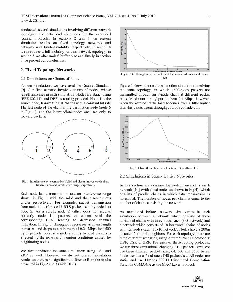
For our simulations, we have used the Qualnet Simulator [9]. Our first scenario involves chains of nodes, whose length increases in each simulation. Nodes are static, using IEEE 802.11b and DBF as routing protocol. Node 1 is the source node, transmitting at 2Mbps with a constant bit rate. The last node of the chain is the destination node (node 6 in Fig. 1), and the intermediate nodes are used only to forward packets.
Fig 1: Interference between nodes. Solid and discontinuous circle show transmission and interference range respectively
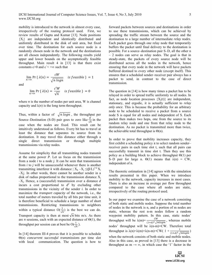
Each node has a transmission and an interference range shown in Fig. 1 with the solid and the discontinuous circles respectively. For example, packet transmission from node 4 interferes with RTS packets sent by node 1 to node 2. As a result, node 2 either does not receive correctly node 1’s packets or cannot send the corresponding CTS, leading to decreased channel utilization. In Fig. 2, throughput decreases as chain length increases, and drops to a minimum of 0.24 Mbps for 1500 bytes packets, because a node’s ability to send packets is affected by the existing contention conditions caused by neighboring nodes.
We have conducted the same simulations using DSR and ZRP as well. However we do not present simulation results, as there is no significant difference from the results presented in Fig.2 and 3 (with DBF).
Fig 2: Total throughput as a function of the number of nodes and packet
size.
Figure 3 shows the results of another simulation involving the same topology, in which 1500-bytes packets are transmitted through an 8-node chain at different packet rates. Maximum throughput is about 0.4 Mbps; however, when the offered traffic load becomes even a little higher than this value, actual throughput drops considerably.
Fig 3: Chain throughput as a function of the offered load
2.2 Simulations in Square Lattice Networks
In this section we examine the performance of a mesh network [10] (with fixed nodes as shown in Fig.4), which consists of parallel chains in which data transmission is horizontal. The number of nodes per chain is equal to the number of chains consisting the network.
As mentioned before, network size varies in each simulation between a network which consists of three horizontal chains with three nodes each (3x3 network) and a network which consists of 10 horizontal chains of nodes with ten nodes each (10x10 network). Nodes have a 200m distance from their neighbors. For each topology, there are three different scenarios, using different routing protocols: DBF, DSR or ZRP. For each of these routing protocols, we run three simulations, changing CBR packets’ size. We use three different packet sizes, 64, 500 and 1500 bytes. Nodes send at a fixed rate of 40 packets/sec. All nodes are static, and use 11Mbps 802.11 Distributed Coordination Function CSMA/CA as the MAC Layer protocol.

IJCSI International Journal of Computer Science Issues, Vol. 7, Issue 4, No 3, July 2010 www.IJCSI.org
3
Fig. 4: Lattice network of 6 chains of nodes with 6 nodes each and 6
horizontal flows
Simulation parameters are presented in Table 1.
Table 1: Simulation Parameters Protocols DBF,DSR,ZRP Simulation time 600 sec Number of nodes 9 to 100 Simulation area 2000x2000 Traffic Type Constant bit rate Packet Size 64,500,1500 bytes Offered load 40 packets/sec Number of connections 3 to 10
In Figure 5, it is shown that as the network size increases, overall throughput is stabilized approximately at 0.1 Mbps, for 1500 bytes packets, which is a value slightly smaller than the one estimated theoretically in [11].
Fig 5: Average per flow throughput in square lattice network as a function of network size and routing protocol for 1500 bytes packets
Figures 6 and 7 show average throughput for 500 and 64 bytes packets respectively.
Fig 6: Average per flow throughput in square lattice network, as a function of network size and routing protocol for 500 bytes packets
Fig 7: Average per flow throughput in square lattice network as a function of network size and routing protocol for 64 bytes packets
Our first observation is that network size and chain length, also mentioned in section 2.1, plays an important role in network performance. When network size and consequently chain length increases, there is a dramatic decrease in per flow throughput. The reason of this behavior is node interference [12], which increases by network size. RTS/CTS handshake cannot eliminate interference caused by hidden nodes, leading to a decrease in networks capacity. Interference range is greater than transmission range, meaning that an interfering signal can cause performance degradation even if its power is less than the power of transmission signal. If we could present analytically simulation results of each single chain, we would notice that in every case, two chains, the one at the top and the other at the bottom of the network perform better than the intermediate ones, justifying that node interference affects network performance.
Another observation is that the three routing protocols have similar behavior regardless of packet size. In all three cases DBF performs better, with ZRP having relatively inferior performance than the other two. A node using DBF forwards its packets through the shortest path, in this case a horizontal chain of nodes. Moreover, because nodes are static there are no invalid routes; packets are correctly forwarded to their destination, making a proactive routing protocol efficient in a square lattice network.
2.3 Simulations in Lattice Networks
In this section we examine two different topologies, both consisting of 18 nodes with a 200m distance between them. The difference between the two scenarios is node placement. In the first case, nodes are placed in three chains consisting of six nodes, whereas in the second configuration we use six chains with three nodes each. The rest of the simulation parameters are the same as in section 2.2.Average per flow throughput values are shown in fig 8.
Solid lines represent the average per flow throughput on a 3x6 network configuration whereas discontinuous line

IJCSI International Journal of Computer Science Issues, Vol. 7, Issue 4, No 3, July 2010 www.IJCSI.org
4
presents the respective of a 6x3 network configuration. Due to the smaller number of nodes per chain in the second case, interference level is decreased, leading to a more effective use of the common medium. DSR benefits from low interference level and due to reactive policy, has the best performance among the three routing protocols.
Fig 8: Average per flow throughput as a function of packet size and routing protocol.
As for the network that consists of 6 chains of three nodes each, its performance is shown by the discontinuous line in fig. 8. We used only one line, because all routing protocols have exactly the same performance. The number of nodes is the same as in the previous case, however the way nodes are placed in the network plays a significant role on networks’ performance. Overall interference is much smaller than in the previous case, therefore performance is not affected by it. As a result all routing protocols perform exactly the same way, regardless the packet size.
3. Lattice Networks with Limited Mobility
3 In order to examine node mobility effects, in this section we present simulation results on two different topologies. In both cases, we assume a lattice network of 36 users, similar to the one in fig.4, distributed in a 1000x1000m area where nodes have 100m distance from their neighbors. The left and right columns of nodes in this network are static, serving as source and destination nodes, respectively. We simulated two different scenarios. In the first one, apart from the static nodes at the edges, there is another static column of nodes, which is the 4th from the left. In the second scenario, the two columns in the middle of the network (3rd and 4th) are static.
In both scenarios simulation time is 600 sec. Nodes follow a random waypoint mobility pattern, with a maximum speed of 10m/s and 30sec pause time. All nodes use 11Mbps 802.11 Distributed Coordination Function CSMA/CA as the MAC Layer protocol. In each scenario nodes use one of the DBF, DSR and ZRP routing protocols. There are 6 Constant bit rate (CBR) traffic source-destination pairs for every routing protocol, using
64, 500 or 1500 bytes packets, sending at a constant rate of 40 packets/sec. We run a total number of 18 simulations scenarios with Table 2 showing the simulation parameters.
Table 2: Simulation Parameters Protocols DBF,DSR,ZRP Simulation time 600 sec Number of nodes 36 Simulation area 1000x1000 Mobility model Random Waypoint Max speed 10m/s Pause time 30sec Traffic Type Constant bit rate Packet Size 64,500,1500 bytes Offered load 40 packets/sec Number of connections 6
Fig.9: Average throughput per flow in limited mobility scenarios.
As shown in fig.9, all protocols attain lower throughput values when small packets are used. DBF and ZRP protocols have similar performance for the same topology and mobility configuration, whereas DSR outperforms them in every case.
Fig. 10 shows average delay per flow. In most of our simulations, when larger size packets are used, the is an increase in packet losses, resulting in lower delay values than those observed when small size packets are used.
Fig.10: Average delay per flow as a function of packet size.
If we compare throughput results presented in figs 5 to 7 for a 6x6 lattice network topology with the results in fig. 9, we observe that there is an increase in throughput when
IJCSI International Journal of Computer Science Issues, Vol. 7, Issue 4, No 3, July 2010 www.IJCSI.org
5
mobility is introduced to the network in almost every case, irrespectively of the routing protocol used. First, we review results of Gupta and Kumar [13]. Node positions {Xi} are independent and identically distributed and uniformly distributed in the disk of unit area, but fixed over time. The destination for each source node is a randomly chosen node in the network and the destinations are all chosen independently. The following results yield upper and lower bounds on the asymptotically feasible throughput. Main result 4 in [13] is that there exist constants c>0 and c΄< +∞ such that
lim Pr
1
and
lim Pr √
0
where n is the number of nodes per unit area, W is channel capacity and λ(n) is the long term throughput.
Thus, within a factor of , the throughput per
Source–Destination (S-D) pair goes to zero like √
in the
case when the nodes are fixed. This result can be intuitively understood as follows. Every bit has to travel at least the distance that separates its source from its destination. It may travel this distance either through a single direct transmission or through multiple transmissions via relay nodes.
Assume for simplicity that all transmitting nodes transmit at the same power P. Let us focus on the transmission from a node i to a node j. It can be seen that transmission from i to j will be unsuccessful whenever there is another transmitting interferer k with distance | Xk –Xj ≤(β/L)1/α Xi
–Xj|. In other words, there cannot be another sender in a disk of radius proportional to the transmission distance Xi
–Xj. Hence, a (successful) transmission over a distance d incurs a cost proportional to d2 by excluding other transmissions in the vicinity of the sender i. In order to maximize the transport capacity of the network, i.e., the total number of meters traveled by all bits per time unit, it is therefore beneficial to schedule a large number of short transmissions. Restricting transmissions to neighbors
within a typical distance O(√
) is the best we can do.
Transport capacity is then at most √ bits m/s. As there are n sessions, each with an expected distance of Θ(1), the
throughput per session can at best be O(√
.
In [14] theorem III-4 proves that it is possible to schedule Θ(n) concurrent successful transmissions per time slot with local communication. The question is how to
forward packets between sources and destinations in order to use these transmissions, which can be achieved by spreading the traffic stream between the source and the destination to a large number of intermediate relay nodes. Each packet goes through one relay node that temporarily buffers the packet until final delivery to the destination is possible. For a source–destination pair S–D, all the other n – 2 nodes can serve as relay nodes. The goal is that in steady-state, the packets of every source node will be distributed across all the nodes in the network, hence ensuring that every node in the network will have packets buffered destined to every other node (except itself). This ensures that a scheduled sender–receiver pair always has a packet to send, in contrast to the case of direct transmission.
The question in [14] is how many times a packet has to be relayed in order to spread traffic uniformly to all nodes. In fact, as node location processes {Xi(t)} are independent, stationary, and ergodic, it is actually sufficient to relay only once. This is because the probability for an arbitrary node to be scheduled to receive a packet from a source node S is equal for all nodes and independent of S. Each packet then makes two hops, one from the source to its random relay node and one from that relay node to the destination. As no packet is transmitted more than twice, the achievable total throughput is Θ(n).
In order to prove that mobility increases capacity, they first exhibit a scheduling policy π to select random sender–receiver pairs in each time slot t, such that all pairs can successfully transmit in time slot t. Then they use this policy as a building block to achieve throughput Θ(1) per S–D pair for large n. Θ(1) means that λ(n) = CW, independent of n.
The theoretic estimation in [14] agrees with the simulation results presented in this paper. When we introduce mobility to the network, capacity increases in most cases. There is also an increase in average per flow throughput compared to the case where all nodes are static, irrespectively of the routing protocol used.
In our paper we examine the case of a network consisting of both static and mobile nodes. Suppose the total number of nodes in the network is n, and a portion of m nodes are static, whereas the rest n-m nodes follow a random waypoint mobility pattern. In this case, static nodes’
throughput will be λ(m)= , whereas mobile
nodes’ throughput will be λ(n-m)=CW. Therefore total
throughput is λ(n)=λ(m)+λ(n-m)=CW( 1 +
)
when the network consists of both static and mobile nodes. Also in this case, as proved in [13] there is a decrease in throughput as m → ∞, in which case the ‘1’ factor in the
IJCSI International Journal of Computer Science Issues, Vol. 7, Issue 4, No 3, July 2010 www.IJCSI.org
6
parenthesis is omitted. Moreover, as the number of static nodes m decreases, there is an increase in throughput, which conforms to the results of [14].
In many cases simulation results agree with the previous theoretic analysis for a network consisting of both static and mobile nodes. However there are cases where there is a difference between theoretical and simulation results. This is expected, as we simulate only a limited number of wireless networks. Moreover, throughput equations in [13] and [14] are approximate, meaning that they do not take into account the differences between routing protocols, or the effect of packets’ size to the network.
4. Random Topology Networks
In this section, we introduce full node mobility and look into the comparative performance of the three routing algorithms in a random topology 11Mbps IEEE 802.11b Ad Hoc network. Simulation area is 1000x1000m and the network consists of 30 users. The network operates in 802.11 Distributed Coordination Function CSMA/CA mode as before. We simulate CBR applications with the same parameters as in section 3 with flows’ destinations chosen randomly from a uniform distribution. Simulation time is 600 sec. We use a RWP mobility model, with a maximum speed of 10m/s and 30sec pause time.
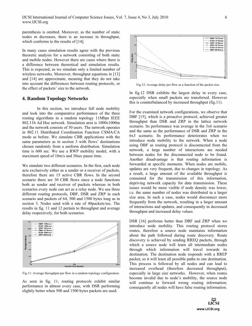
We simulate two different scenarios. In the first, each node acts exclusively either as a sender or a receiver of packets, therefore there are 15 active CBR flows. In the second scenario there are 30 CBR flows since a node functions both as sender and receiver of packets whereas in both scenarios every node can act as a relay node. We use three different routing protocols, DBF, DSR and ZRP in each scenario and packets of 64, 500 and 1500 bytes long as in section 3. Nodes send with a rate of 40packets/sec. The results in fig. 11 and 12 pertain to throughput and average delay respectively, for both scenarios.
Fig.11: Average throughput per flow in a random topology configuration.
As seen in fig. 11, routing protocols exhibit similar performance in almost every case, with DSR performing slightly better when 500 and 1500 bytes packets are used.
Fig.12: Average delay per flow as a function of the packet size.
In fig.12 DSR exhibits the largest delay in every case, especially when small packets are transferred. However this is counterbalanced by increased throughput (fig.11).
For the examined network configurations, we observe that DBF [15], which is a proactive protocol, achieved greater throughput than DSR and ZRP in the lattice network scenario. Its performance was average in the 3x6 scenario and the same as the performance of DSR and ZRP in the 6x3 scenario. Its performance deteriorates when we introduce node mobility to the network. When a node using DBF as routing protocol is disconnected from the network, a large number of interactions are needed between nodes for the disconnected node to be found. Another disadvantage is that routing information is forwarded at specific moments. When nodes are mobile, updates are very frequent, due to changes in topology. As a result, a large amount of the available throughput is consumed for the transmission of this information, depriving network capacity for data transmission. These issues would be more visible if node density was lower, i.e. the same number of nodes was distributed in a larger size area. In such a case, nodes would disconnect more frequently from the network, resulting in a larger amount of interactions and updates, and consequently in decreased throughput and increased delay values.
DSR [16] performs better than DBF and ZRP when we introduce node mobility. This routing protocol stores routes, therefore a source node maintains information about the path followed during route discovery. Route discovery is achieved by sending RREQ packets, through which a source node will learn all intermediate nodes through which information will travel towards its destination. The destination node responds with a RREP packet, so it will learn all possible paths to one destination. This process is followed by all nodes and can lead to increased overhead (therefore decreased throughput), especially in large size networks. However, when routes become invalid due to node’s mobility, the source node will continue to forward wrong routing information; consequently all nodes will have false routing information.
IJCSI International Journal of Computer Science Issues, Vol. 7, Issue 4, No 3, July 2010 www.IJCSI.org
7
In terms of delay, DSR shows greater delay in the simulated scenario of section 4, where all nodes move and the offered load is increased compared to the scenarios of section 3. This shows that DSR is sensitive to network load and mobility conditions.
When the ZRP routing protocol is used, its performance is slightly better than the performance of DBF in many cases. As mentioned before, ZRP defines zones whose radius is the maximum number of neighbor users. In this zone, IARP [17] (Intrazone Routing Protocol) protocol is used, making route requests easier without examining all nodes in the network. The amount of unused routing information is also decreased. Distant nodes can be accessed through reactive routing, using IERP [17] (Interzone Routing Protocol) protocol. ZRP’s advantage is that local topology is known. This way when there is an unstable connection, packets are forwarded through an alternative path. Moreover, this can be used to reduce path length, in case the distance between two nodes is reduced. This explains the slight difference in performance compared to DBF. Most nodes are relatively close to one another, implying that in many cases proactive routing is used, similar to DBF. Reactive routing is used for distant nodes-destinations, leading to increased throughput in this case. Due to node mobility, network topology must be rediscovered many times, which leads to an increase in delay, due to topology information exchange between nodes. Choosing zone radius is a tradeoff between routing efficiency and control information in order for the zone to become known. In our simulations, we choose a zone radius which systematically decreases the amount of required control information.
Similar behavior, though improved in terms of throughput and packet losses, is observed when an FTP application is used (instead of CBR) in the simulated scenarios described. Another important aspect is that in most cases where mobility is introduced, we observe large delays when small packets are transferred. We conducted several simulations in order to explain this behavior. Our first conclusions are that in this case, buffer size plays significant role in delay. By decreasing a node’s buffer size, there is a significant decrease in delay, and in some cases, an increase in throughput is observed. Analytical results are presented in section 5.
Regarding packet losses, in the course of a packet’s transmission, a source node counts the numbers of short (ns) and long (nl) retries. Let a source node transfer a DATA frame with a packet of length equal to or less than the RTS threshold P, or an RTS frame. If a correct ACK or CTS frame, respectively, is received within timeout limits, then the ns-counter is zeroed; otherwise ns is advanced by one. Similarly, the nl-counter is zeroed or advanced by one
in case of reception or absence of a correct ACK frame (within timeout) confirming the successful transfer of a DATA frame with a packet of length greater than P. When any of ns and nl attains its limit Ns or Nl respectively, the current packet is rejected. After the rejection or success of a packet transmission, nr, ns, and nl values are zeroed [18]. Limits defined by IEEE 802.11b are 7 and 4 for ns and nl
respectively. We used these values in our simulations. However we do not present packet loss results in this paper, due to page limitations, and will be presented in a future extended work.
5. Simulations Altering Buffer Size
In section 2.2 we conducted simulations on lattice networks which consist of chains of nodes. We present throughput results showing that as the number of nodes of a chain increases, therefore network size increases, there is a decrease in average per flow throughput which leads to stabilization of throughput value.
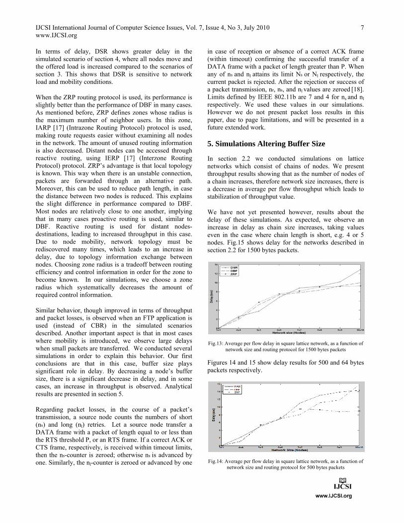
We have not yet presented however, results about the delay of these simulations. As expected, we observe an increase in delay as chain size increases, taking values even in the case where chain length is short, e.g. 4 or 5 nodes. Fig.15 shows delay for the networks described in section 2.2 for 1500 bytes packets.
Fig.13: Average per flow delay in square lattice network, as a function of network size and routing protocol for 1500 bytes packets
Figures 14 and 15 show delay results for 500 and 64 bytes packets respectively.
Fig.14: Average per flow delay in square lattice network, as a function of network size and routing protocol for 500 bytes packets

IJCSI International Journal of Computer Science Issues, Vol. 7, Issue 4, No 3, July 2010 www.IJCSI.org
8
As shown by figures 13-15, average delay value increases for each network size as the size of transferred packets decreases, especially when network size is greater than 6x6. However the most remarkable observation is that in those cases delay gets greater values when small packets are transferred through the network, e.g. 64 bytes packets, rather than when large size packets, e.g. 1500 bytes packets are transferred. This behavior can be explained through an analysis of buffer size. In our simulations we used a buffer of 50000 bytes and FIFO queuing scheme is used. When 64 bytes packets are used, a larger amount of packets can be stored in buffer, compared to the case when 1500 bytes packets are transferred through the network. Therefore in the first case of 64 bytes packets, a greater amount of time is required in order for those packets to be stored, processed and forwarded to the next hop.
Fig.15: Average per flow delay in square lattice network, as a function of network size and routing protocol for 64 bytes packets
When network size is small, as in the cases of 3x3 and 4x4 as shown in figures 13 – 15, the total amount of packets is decreased compared to the rest of the cases. Due to the decreased amount of packets in the network it is harder for buffers to get fully loaded, therefore delay is considerably decreased. However, in the rest cases when the total amount of packets is increased, more packets are stored in a nodes’ buffer leading to very large delay values. Of course there are differences in these values which depend on the routing protocol used; however there is no dispute that all simulated routing protocols follow this behavior.
In order to examine the validity of these results in relation to packet size, we conducted the same simulation using 280 bytes and 1000 bytes packets. The results of these simulations show that all routing protocols follow similar behavior to the one observed in figures 13 to 15.
Our first conclusion is that delay increases when small size packets are transferred through the network and it decreases as packets of larger size are used. We made the assumption that this behavior happens due to the number of packets stored in buffer. When small packets are
transferred a greater amount of packets are stored in buffer rather than in the case of large size packets leading to an increase in delay. In order to check if our speculation is correct, we conduct similar simulations to the ones presented in section 2.2. The only difference in this case is that we change buffer size. Until now we used a buffer size of 50000 bytes, whereas now we change buffer size. Buffer size depends on the size of packets we use. Figures 16 and 17 present simulation results for 64 bytes packets for 5000, 500 and 128 bytes buffer size respectively.
Fig.16: Average per flow delay in square lattice network, with horizontal flows, as a function of network size and routing protocol for 64 bytes
packets for 5000 and 500 bytes buffer size.
Fig.17: Average per flow delay in square lattice network, with horizontal flows, as a function of network size and routing protocol for 64 bytes
packets and 128 bytes buffer size.
As shown in fig. 16 and 17 there is a decrease in delay as buffer size decreases, especially when buffer size is 5000 and 500 bytes. In the last case, for 128 bytes buffer size, ZRP and DBF appear to have increased delay compared to DSR protocol, however even in this case delay is severely decreased compared to the case of 50000 bytes buffer.
For further confirmation of our results we present similar results for 500 and 1500 bytes packets in the following figures. In every case, there is a decrease in delay when a smaller size buffer is used. In the case of 500 bytes packets we used 1500 and 500 buffer size, while when 1500 bytes

IJCSI International Journal of Computer Science Issues, Vol. 7, Issue 4, No 3, July 2010 www.IJCSI.org
9
packets are transferred our simulations where conducted using 5000 and 3000 bytes buffers.
It is more than obvious that when buffer size is decreased there is a severe decrease in average per flow delay, especially when network size is increased. In our simulations this is clearly observed when network size is 6x6 or 7x7.
Fig.18: Average per flow delay in square lattice network, with horizontal flows, as a function of network size and routing protocol for 500 bytes
packets and 5000 and 1500 bytes buffer size.
Of course this conclusion is not very safe when buffer size is such that only an extremely limited number of packets can be stored in, as in the case presented in fig 17. In this case, packets of 64 bytes are transferred through the network, and buffer size is 128 bytes. Therefore, only 2 packets can be stored in a node’s buffer. In this case, when DSR and DBF routing protocols are used delay is almost equal to the delay presented in fig 6 for the respective routing protocols. However when the routing protocol is ZRP, delay is almost 10 to 12 times increased compared to the other routing protocols, even for networks of average size, showing that routing protocol has an important role in network’s performance. However, limiting buffer size still appears to be an effective way of decreasing delay.
Fig.19: Average per flow delay in square lattice network, with horizontal flows, as a function of network size and routing protocol for 500 bytes
packets for 5000 and 1500 bytes buffer size.
Another aspect which needs to be examined is the impact buffer decrease has on throughput. When buffer size is decreased, the maximum amount of packets a buffer can store is decreased. Simulation results already presented, show that such a decrease is beneficial in terms of delay. However by decreasing buffer’s capacity, the possibility of packets to be dropped is increased, leading to throughput deterioration, although we managed to improve delay by decreasing it.
Fig. 20 presents throughput simulation results when 1500 bytes packets are transferred through the network.
Fig 20: Average per flow throughput in square lattice network, with horizontal flows, as a function of network size and routing protocol for
1500 bytes packets, for 5000 and 1500 bytes buffer size.
Those results compared to the simulation results in fig. 6, show that in most cases there is an increase in per flow throughput as buffer size decreases. Especially minimum throughput values are considerably improved when smaller size buffer is used. Our conclusion is that when smaller size buffer is used there is a decrease in delay without an impact in throughput. Contrarily in most cases there is an increase in throughput, which leads to an overall improvement in a network’s performance.
6. Conclusions
Our focus in this paper is to evaluate the performance of an Ad Hoc network, in scenarios involving both static and mobile nodes, using different routing protocols and offered load conditions. We compare three different routing protocols, each representing one of the three types of routing protocols, i.e., proactive, reactive and hybrid. Our main contribution (relative to previous work) is the systematic analysis of these routing protocols in a variety of network topologies including static nodes scenarios, scenarios with limited node mobility and full node mobility (sections 2, 3, 4 respectively), citing a simple throughput theoretical analysis for each of those topologies.

IJCSI International Journal of Computer Science Issues, Vol. 7, Issue 4, No 3, July 2010 www.IJCSI.org
10
Our first observation is that, per flow throughput is affected by the way nodes are placed in the network. Moreover, a node’s and a network’s performance is affected by node mobility and the choice of routing protocols. We showed that in a network configuration where all nodes are mobile and there is an increased traffic load to be transmitted, per node throughput is increased when a reactive routing protocol is employed, especially when larger data segments are transmitted.
In terms of comparative performance evaluation, we show advantages of reactive routing protocols such as DSR, leading to increased throughput achieved when nodes are mobile, at the expense of increased delay. The efficiency in route discovery contributes to increased delay in this case. As for proactive and hybrid routing protocols, DBF and ZRP respectively, there seems to be relatively small difference between them. ZRP shows some advantages compared to DBF when nodes are mobile in which its proactive routing component performs better than reactive routing. However DBF is more effective in the case of static chains of nodes or in square lattice networks.
Moreover we examined the effect of buffer size in both static and mobile lattice networks’ performance. In our simulations, reducing buffer size causes delay reduction and throughput improvement for all routing protocols. Especially when DSR and DBF routing protocols are used there is an increase in throughput even for small size networks, while in the case of ZRP routing protocol, throughput decreases slightly for small size networks when buffer size decreases. However even in the case of ZRP, while the size of buffer decreases there is an increase in throughput as network size grows bigger.
References [1] M. Abolhasan, T. Wysocki, “A review of routing protocols for mobile ad hoc networks”, Ad Hoc Networks, Vol. 2, Issue 1, pp 1-22, 1 January 2004. [2] R. Misra, C. R. Mandal, “Performance comparison of AODV/DSR on-demand routing protocols for ad hoc networks in constrained situation”, IEEE Int. Conf. on Personal Wireless Communications, pp. 86- 89, Jan. 2005. [3] G. Jayakumar, G. Ganapathy, “Performance Comparison of Mobile Ad-hoc Network Routing Protocol”, Int. J. of Comp. Science and Net. Security, Vol.7, No.11, Nov. 2007. [4] H. Jiang and J. J. Garcia-Luna-Aceves, “Performance comparison of three routing protocols for ad hoc networks”, Proceeding of IEEE ICCCN 2001. [5] P. Johansson, T. Larsson, N. Hedman, B. Mielczarek, and M. Degermark, “Scenario-Based Performance Analysis of Routing Protocols for Mobile Ad Hoc Networks”, 5th ACM/IEEE Int. Conf. on Mobile computing and networking, pp. 195-206. 1999. [6] J. Broch, D. A. Maltz, D. B. Johnson, Y. Hu, J. Jetcheva, "A Performance Comparison of Multi-Hop Wireless Ad Hoc Network Routing Protocols", Proc. of the 4th ACM/IEEE Int. conf. on Mobile computing and networking, pp. 85-97. 1998. [7] Li Layuan, Li Chunlin, Yaun Peiyan, “Performance evaluation and simulations of routing protocols in ad hoc networks”, Computer Communications, Vol. 30 . pp 1890–1898. 2007
[8] Azzedine Boukerche, “Performance Evaluation of Routing Protocols for Ad Hoc Wireless Networks”, Journal of Mobile Networks and Ap. Vol. 9, No 4. pp.333-342, 2004. [9] Qualnet , www.scalable-networks.com [10] I.F. Akyildiz, Xudong Wang, “A survey on wireless mesh networks”, IEEE Communications Magazine, Vol. 43, Issue 9, pp. S23 - S30, Sept. 2005 [11] J. Li, C. Blake Douglas,S. J. De Couto, H. I. Lee, R. Morris, “Capacity of Ad Hoc Wireless Networks”, 7th annual international conference on Mobile computing and networking, 2001. [12] Kaixin Xu, Mario Gerla, Sang Bae . “How Effective is the IEEE 802.11 RTS/CTS Handshake in Ad Hoc Networks?”, Proceeding of GLOBECOM’02.
[13] P. Gupta, P. R. Kumar, “The capacity of wireless networks,” IEEE Transactions on Information Theory, vol. 46, no. 2, Mar 2000 [14] M. Grossglauser, D. N. C. Tse, “Mobility increases the capacity of Ad Hoc wireless networks” , IEEE/ACM Transactions on Networking, Vol. 10, No. 4, 2002. [15] D. Bertsekas,R. Gallaher, “Data Networks”, Second Edition, Prentice Hall,1992. [16] J . Wu, “An Extended Dynamic Source Routing Scheme in Ad Hoc Wireless Networks”,HICSS, 2002. [17] Z. Haas, M. Pearlman, P. Samar, “The Zone Routing Protocol (ZRP) for Ad Hoc Networks,” IETF InternetDraft,draft-ietf-manet-zone-zrp-04.txt, July 2002. [18] Andrey Lyakhov, Florian Simatos “Hybrid RTS/CTS mechanism in Wi-Fi Ad Hoc Networks with Correlated Channel Failures”, 17th IMACS, 2005 Evaggelos C. Chatzistavros received his diploma of Computer and Electrical Engineer from Democritus University oh Thrace, Greece, in 2007, has completed his M. Sc thesis on “Performance evaluation of routing protocols in IEEE Ad Hoc networks” from the Department of Electrical and Computer Engineering, Democritus University of Thrace, in 2010 and is currently working on his Ph. D thesis. His research interests are communication networks, wireless networks and performance evaluation of routing protocols. George Stamatelos is an assistant professor of Electrical and Computer Engineering in Democritus University of Thrace. He received his Ph.D. in EECS from Concordia University, Montreal, Canada in 1992 and has since held various positions in both the academia and industry. He teaches courses in Telecommunications and Computer Networks and his research interests include stochastic processes, queuing theory, communication networks and nomadic computing.
IJCSI International Journal of Computer Science Issues, Vol. 7, Issue 4, No 3, July 2010 ISSN (Online): 1694-0784 ISSN (Print): 1694-0814
11
Design of Radial Basis Function Neural Networks for Software Effort Estimation
Ali Idri1, Abdelali Zakrani1 and Azeddine Zahi2
1 Department of Software Engineering, ENSIAS, Mohammed Vth –Souissi University, BP. 713, Madinat Al Irfane, Rabat, Morocco
2 Department of Computer Science, FST, Sidi Mohamed Ben Abdellah University,
B.P. 2202, Route d’Imouzzer, Fès, Morocco
Abstract In spite of the several software effort estimation models developed over the last 30 years, providing accurate estimates of the software project under development is still unachievable goal. Therefore, many researchers are working on the development of new models and the improvement of the existing ones using artificial intelligence techniques such as: case-based reasoning, decision trees, genetic algorithms and neural networks. This paper is devoted to the design of Radial Basis Function Networks for software cost estimation. It shows the impact of the RBFN network structure, especially the number of neurons in the hidden layer and the widths of the basis function, on the accuracy of the produced estimates measured by means of MMRE and Pred indicators. The empirical study uses two different software project datasets namely, artificial COCOMO’81 and Tukutuku datasets. Keywords: software effort estimation, RBF Neural Networks, COCOMO'81, Tukutuku dataset.
1. Introduction
As demand for software computer increases continually and the software scope and complexity become higher than ever, the software companies are in real need of accurate estimates of the project under development. Indeed, good software effort estimates are critical to both companies and clients. They can be used for making request for proposals, contract negotiations, planning, monitoring and control [1]. Unfortunately, many software development estimates are quite inaccurate. Molokken and Jorgensen report in recent review of estimation studies that software projects expend on average 30-40% more effort than is estimated [2]. In fact, if the project is underestimated, once it seems running out of the schedule, the project manager and his team are put under high pressure to finish the software. As a result, the manager may skimp on verification and validation or quality assurance. For example, developers might scrap unit testing or software integration and test or
rush a premature design into production [3]. Consequently, the delivered product may be with poor quality and many underdeveloped functions. On the other side, if the project is overestimated, hence according to Parkinson’s Law, the work will expand to fill available time, which leads the company to miss opportunities to take on other projects. In order to help solving the problems of making some accurate software project predictions and supporting managers in their task, many estimation models have been developed over the last three decades [4], falling into three general categories [5][6]: Expert judgment: This technique evolves the consultation of one expert in order to derive an estimate for the project based on his experience and available information about the project under development. This technique has been used extensively. However, the estimates are produced in intuitive and non-explicit way. Therefore, it is not repeatable. According to Gray et al. [7] although expert judgment is always difficult to quantify, it can be an effective estimate tool to adjust algorithmic models. Algorithmic models: These are the most popular models in the literature. They are based on mathematical formulae linking effort with effort drivers to produce an estimate of the project. Usually the principal effort driver used in these models is software size (FP, source lines of code…). They need to be calibrated to local circumstances. Machine learning: The machine learning approaches were appeared at the beginning of nineties to overcome the drawbacks of the two previous categories. Examples of these approaches include regression trees [8] [9], fuzzy logic [1] [10], case based reasoning [6] [11], and artificial neural networks [12] [13] [14] [15]. This paper is concerned with the design of the neural networks approach, especially radial basis function neural

IJCSI International Journal of Computer Science Issues, Vol. 7, Issue 4, No 3, July 2010 www.IJCSI.org
12
networks, for development effort estimation models. Artificial neural networks are recognized for their ability to produce good results when dealing with problems where there are complex relationships between inputs and outputs, and where the inputs are distorted by high noise levels [14]. The use of Radial Basis Function neural Networks (RBFN) in software effort estimation requires the determination of the structure of these latter and the adjustment of their parameters. A critical step among the RBF networks configuration is the determination of the optimal structure of the hidden layer. In particular the number of hidden neurons and the formulae used to compute the widths of these kernels functions. In our earlier work [15], we have conducted an empirical study using two different designs of RBFN networks, one time using APC-III clustering algorithm to construct the hidden layer and another time using the well-known algorithm K-means. The results obtained suggest that RBFN with K-means performs better than that with APC-III in terms of accuracy measures MMRE and Pred. In addition, the results showed that the accuracy of RBFN depends also on classification used in the hidden layer. For instance, the classification obtained by minimizing objective function J leads to better estimates than that obtained by maximizing Dunn index D1. The main goal of the present paper is to experiment two designs of RBF neural networks for software effort estimation. It focuses on the impact of the widths of the Gaussian functions on accuracy of estimates generated by RBFN network. The remaining of this paper is organized as follows. Section 2 reviews the basic principles of a RBF neural network. Section 3 tackles the description of datasets used to perform our empirical study and evaluation criteria adopted to compare the predictive accuracy of the designed models. Section 4 focuses on the configuration of the proposed RBF network. Section 5 presents and discusses the obtained results, and finally, in Section 6 we provide a number of concluding comments.
2. RBF Neural Networks
The architecture of RBFN Neural Network is quite simple. It involves three different layers. An input layer which consists of sources nodes (cost drivers); a hidden layer in which each neuron computes its output using a radial basis function, which is in general a Gaussian function, and an output layer which builds a linear weighted sum of hidden neuron outputs and supplies the response of the network (effort). A RBF neural network configured for software effort estimation has only one output neuron. So, it
implements the output-input relation in Eq. (1) which is indeed a composition of the nonlinear mapping realized by the hidden layer with the linear mapping realized by the output layer
1
where M is the number of hidden neurons, is the input, are the output layer weights of the RBFN networks and is Gaussian radial basis function given by:
e 2 where and are the center and the width of hidden neuron respectively and . denotes the Euclidean distance.
Fig. 1 Radial Basis Function Network architecture for software
development effort estimation
3. Data Description and Evaluation Criteria
This section describes the datasets used to perform the empirical study, and presents also the evaluation criteria adopted to compare the estimating capability of the developed models.
3.1 Data Description
The data used in the present study comes from two sources namely, from the COCOMO'81 dataset published by Boehm in his seminal book "software engineering economics" [16] and from Tukutuku dataset. The Artificial COCOMO’81 dataset is generated artificially from the original one. It contains 252 software projects which are mostly scientific applications developed by Fortran [16]; Each project is described by 13 attributes (see Table 1) : the software size measured in KDSI (Kilo

IJCSI International Journal of Computer Science Issues, Vol. 7, Issue 4, No 3, July 2010 www.IJCSI.org
13
Delivered Source Instructions) and the remaining 12 attributes are measured on a scale composed of six linguistic values: ‘very low’, ‘low’, ‘nominal’, ‘high’, ‘very high’ and ‘extra high’. These 12 attributes are related to the software development environment such as the experience of the personnel involved in the software project, the method used in the development and the time and storage constraints imposed on the software.
Table 1: Software attributes for COCOMO'81dataset Software attributes
Description
SIZE Software Size
DATA Database Size
TIME Execution Time Constraint
STOR Main Storage Constraint
VIRTMIN Virtual Machine Volatility
VIRT MAJ Virtual Machine Volatility
TURN Computer Turnaround
ACAP Analyst Capability
AEXP Applications Experience
PCAP Programmer Capability
VEXP Virtual Machine Experience
LEXP Programming Language Experience
SCED Required Development
The Tukutuku dataset contains 53 Web projects [17]. Each Web application is described using 9 numerical attributes such as: the number of html or shtml files used, the number of media files and team experience (see Table 2). However, each project volunteered to the Tukutuku database was initially characterized using more than 9 software attributes, but some of them were grouped together. For example, we grouped together the following three attributes: the number of new Web pages developed by the team, the number of Web pages provided by the customer and the number of Web pages developed by a third party (outsourced) in one attribute reflecting the total number of Web pages in the application (Webpages).
Table 2: Software attributes for Tukutuku dataset
Attributes Description
Teamexp Average number of years of experience the team has on Web development
Devteam Number of people who worked on the software project
Webpages Number of web pages in the application
Textpages Number of text pages in the application (text page has 600 words)
Img Number of images in the application
Anim Number of animations in the application
Audio/video Number of audio/video files in the application
Tot-high Number of high effort features in the application
Tot-nhigh Number of low effort features in the application
3.2 Evaluation Criteria
We employ the following criteria to assess and compare the accuracy of the effort estimation models. A common criterion for the evaluation of effort estimation models is the magnitude of relative error (MRE), which is defined as
3
The MRE values are calculated for each project in the datasets, while mean magnitude of relative error (MMRE) computes the average over N projects
1
4
Generally, the acceptable target value for MMRE is 25%. This indicates that on the average, the accuracy of the established estimation models would be less than 25%. Another widely used criterion is the Pred(l) which represents the percentage of MRE that is less than or equal to the value l among all projects. This measure is often used in the literature and is the proportion of the projects for a given level of accuracy. The definition of Pred(l) is given as follows:
5
Where N is the total number of observations and k is the number of observations whose MRE is less or equal to l. A common value for l is 0.25, which also used in the present study. The Pred(0.25) represents the percentage of projects whose MRE is less or equal to 25%. The Pred(0.25) value identifies the effort estimates that are generally accurate whereas the MMRE is fairly conservative with a bias against overestimates.
4. RBF Network Construction
As we have mentioned earlier in this paper, the use of RBF neural network to estimate software development effort requires the determination of the network architecture and its parameters, namely the number of input and hidden neurons, the centers , widths , and the weights . The number of the input neurons is, usually and simply, the number of the attributes describing the historical

IJCSI International Journal of Computer Science Issues, Vol. 7, Issue 4, No 3, July 2010 www.IJCSI.org
14
software projects in the used dataset. Therefore, when applying RBF network to COCOMO’81, the number of input neurons is equal to 9 and in the case of Tukutuku dataset, the number of input neurons is equal to 13. Concerning the number of hidden neurons, C, is determined using clustering algorithms. The following subsection deals with the initialization of the centers of hidden layer by means of k-means algorithm.
4.1 Construction of the Hidden Layer of RBFN
The construction of hidden layer of the proposed network is achieved using clustering techniques. The role of clustering in the design of RBFN is to set up an initial distribution of receptive fields (hidden neurons) across the input space of the input variables (software attributes). In literature, clustering techniques have been successfully used in the configuration of the hidden layer of RBFN [18] [19]. K-means clustering algorithm, developed by MacQueen in 1967 [20], is a popular clustering technique which is used in numerous applications. It is a multi-pass clustering algorithm. The k-means algorithm partitions a collection of N vectors into c clusters , i=1,..,c. The aim is to find cluster centers (centroids) by minimizing a dissimilarity (or distance) function which is given in below.
, 6
where is the center of cluster ; , is the distance between ith center and kth data point ( ). For simplicity, the Euclidean distance is used as dissimilarity measure and the overall dissimilarity function is expressed as follows.
7
The outline of the k-means algorithm can be stated as follows:
1- Define the number of the desired clusters, C. 2- Initialize the centers , i=1..C. This is typically
achieved by randomly selecting c points from among all of the data points.
3- Compute the Euclidean distance between and , j=1..N and i=1..c
4- Assign each to the most closer cluster 5- Recalculate the centers 6- Compute the objective function J given in Eq. (7).
Stop if its improvement over previous iteration is below a threshold.
7- Iterate from step 3.
The above k-means based initialization process produces a set of centers , which are the kernels of Gaussian basis function.
4.2 Computation of the widths
One of the most important aspects to be addressed is the determination of the widths of unit function and its inherent complexity [21]. These parameters control the amount of overlapping of kernels functions as well as the network generalization. Small values lead a rapidly decreasing function while a larger values result in more varying function. Hence, it is clear that the setting of the widths ( σ is critical step to the RBF network generalization. To address this issue, many heuristics and techniques based on solid mathematical concepts have been proposed in the literature [21] [22] [23]. The main idea is to determine σ in order to cover the input space as uniformly as possible [19]. However, covering the historical software project space uniformly implies that the RBFN will be able to generate an estimate for a new project even though it is not similar to any historical project. In such a situation, we prefer that the RBFN does not provide any estimate than one that may easily lead to wrong managerial decisions and project failure. In [24] and [25], we have adopted a simple strategy based primarily on assigning one value to all σ . In the present paper we are interested in studying the impact of the widths on the accuracy of RBFN. The empirical study uses the following formulae:
max , , 1
max/
, 1 8
max , , 1
min/
, 1 9
where Card C is the cardinality of cluster .
4.3 Computation of weights
Provided that the centers and the widths of the basis functions have been determined, the weights of the output layer can be calculated and adjusted using a well-known supervised learning algorithm Backpropagation, which based on following formula: Δ 10 where is the learning rate and is the output of the jth basis function of the hidden layer.

IJCSI International Journal of Computer Science Issues, Vol. 7, Issue 4, No 3, July 2010 www.IJCSI.org
15
5. Overview of Empirical Results
The following section presents and discusses the results obtained when applying the RBFN to the artificial COCOMO’81 and Tukutuku datasets. The calculations were made using two software prototypes developed with C language under a Microsoft Windows PC environment. The first software prototype implements the k-means clustering algorithm, providing the clusters and their centers from the used dataset. The second software prototype implements a cost estimation model based on an RBFN architecture in which the hidden layer parameters are determined by means of the first software prototype. The two datasets used to carry out the empirical study were prepared and analyzed. For example all numeric types of effort drivers were normalized within 0 to 1 in both datasets in order to have the same degree of influence. Afterwards, we conducted several experiments using different configurations of RBFN. These experiments use the full dataset for training and testing. The
5.1 COCOMO'81 dataset
Our first experiment is performed using COCOMO’81 dataset containing 252 historical software projects. Two models of RBF networks were designed to examine the impact of basis function widths on accuracy of estimates produced by the network. The first RBFN effort estimation model uses the formula of widths given in Eq. (8) and the second model uses the formula of widths given in Eq. (9).
Model 1: , Model 2: ,
From each model, different configurations have been obtained by varying the number of hidden neurons C. the aim was to determine which widths formula improve the estimates. So, we have trained and tested the above models using COCOMO’81 dataset. The learning rate was set to 0.03 for the all experiments in this paper. Fig. 2 shows and compares the results of the two models. From this figure we note that the RBFN models using
generate a lower MMRE than that using for each number of hidden neurons. For example, for C=120 the model 1 made a higher prediction error (MMRE=60.81) than the Model 2 (MMRE=34.96). Then, in terms of MMRE, Model 2 performs better than Model 1.
Fig. 2 Relationship between the accuracy of RBFN (MMRE) and used classification k-means for COCOMO'81 dataset.
Fig. 3 compares the accuracy of the two above models, in terms of Pred(0.25), when varying the number of hidden neurons. As can be seen, the accuracy of RBF networks using performs much better than RBF Networks using . Indeed, the Model 1 produced poor estimates even when increasing the number of hidden neurons until 160. Whereas Model 2 generates acceptable effort estimates with a number of hidden neurons C=120.
Fig. 3 Relationship between the accuracy of RBFN (Pred) and the used formula of σ according to the number of hidden neurons.
Table 3 shows the results obtained using different configurations of RBF networks.
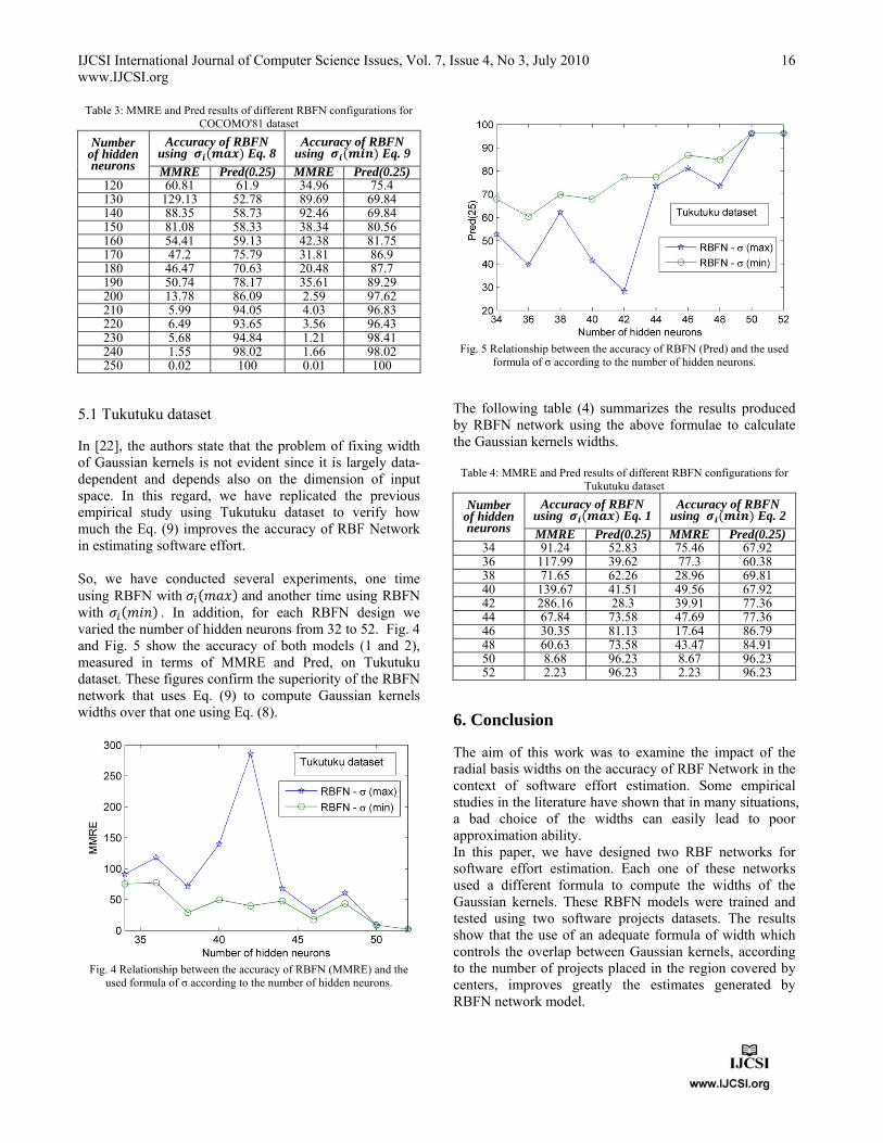
IJCSI International Journal of Computer Science Issues, Vol. 7, Issue 4, No 3, July 2010 www.IJCSI.org
16
Table 3: MMRE and Pred results of different RBFN configurations for COCOMO'81 dataset
Number of hidden neurons
Accuracy of RBFN using Eq. 8
Accuracy of RBFN using Eq. 9
MMRE Pred(0.25) MMRE Pred(0.25)120 60.81 61.9 34.96 75.4130 129.13 52.78 89.69 69.84140 88.35 58.73 92.46 69.84150 81.08 58.33 38.34 80.56160 54.41 59.13 42.38 81.75170 47.2 75.79 31.81 86.9180 46.47 70.63 20.48 87.7190 50.74 78.17 35.61 89.29200 13.78 86.09 2.59 97.62210 5.99 94.05 4.03 96.83220 6.49 93.65 3.56 96.43230 5.68 94.84 1.21 98.41240 1.55 98.02 1.66 98.02250 0.02 100 0.01 100
5.1 Tukutuku dataset
In [22], the authors state that the problem of fixing width of Gaussian kernels is not evident since it is largely data-dependent and depends also on the dimension of input space. In this regard, we have replicated the previous empirical study using Tukutuku dataset to verify how much the Eq. (9) improves the accuracy of RBF Network in estimating software effort. So, we have conducted several experiments, one time using RBFN with and another time using RBFN with . In addition, for each RBFN design we varied the number of hidden neurons from 32 to 52. Fig. 4 and Fig. 5 show the accuracy of both models (1 and 2), measured in terms of MMRE and Pred, on Tukutuku dataset. These figures confirm the superiority of the RBFN network that uses Eq. (9) to compute Gaussian kernels widths over that one using Eq. (8).
Fig. 4 Relationship between the accuracy of RBFN (MMRE) and the used formula of σ according to the number of hidden neurons.
Fig. 5 Relationship between the accuracy of RBFN (Pred) and the used formula of σ according to the number of hidden neurons.
The following table (4) summarizes the results produced by RBFN network using the above formulae to calculate the Gaussian kernels widths.
Table 4: MMRE and Pred results of different RBFN configurations for Tukutuku dataset
Number of hidden neurons
Accuracy of RBFN using Eq. 1
Accuracy of RBFN using Eq. 2
MMRE Pred(0.25) MMRE Pred(0.25)34 91.24 52.83 75.46 67.9236 117.99 39.62 77.3 60.3838 71.65 62.26 28.96 69.8140 139.67 41.51 49.56 67.9242 286.16 28.3 39.91 77.3644 67.84 73.58 47.69 77.3646 30.35 81.13 17.64 86.7948 60.63 73.58 43.47 84.9150 8.68 96.23 8.67 96.2352 2.23 96.23 2.23 96.23
6. Conclusion
The aim of this work was to examine the impact of the radial basis widths on the accuracy of RBF Network in the context of software effort estimation. Some empirical studies in the literature have shown that in many situations, a bad choice of the widths can easily lead to poor approximation ability. In this paper, we have designed two RBF networks for software effort estimation. Each one of these networks used a different formula to compute the widths of the Gaussian kernels. These RBFN models were trained and tested using two software projects datasets. The results show that the use of an adequate formula of width which controls the overlap between Gaussian kernels, according to the number of projects placed in the region covered by centers, improves greatly the estimates generated by RBFN network model.

IJCSI International Journal of Computer Science Issues, Vol. 7, Issue 4, No 3, July 2010 www.IJCSI.org
17
References [1] M. W. Nisar, and Y.-J. Wang, and M. Elahi, "Software
Development Effort Estimation Using Fuzzy Logic - A Survey", in 5th International Conference on Fuzzy Systems and Knowledge Discovery, 2008, pp. 421-427.
[2] K. Molokken, and M. Jorgensen, "A Review of Surveys on Software Effort Estimation", in International Symposium on Empirical Software Engineering, 2003, pp. 223-231.
[3] T. Menzies, and J. Hihn, "Evidence-Based Cost Estimation for Better-Quality Software", IEEE Software, Vol. 23, No. 4, 2006, pp. 64-66.
[4] M. Jorgensen, and M. Shepperd, "A Systematic Review of Software Development Cost Estimation Studies", IEEE Transactions on Software Engineering, Vol. 33, No. 1, 2007, pp. 33-53.
[5] M. J. Shepperd, and C. Schofield, and B. Kitchenham, "Effort Estimation Using Analogy", in International Conference on Software Engineering, 1996, pp. 170-178.
[6] E. Mendes, and I. D. Watson, and C. Triggs, and S. Counsell, "A Comparative Study of Cost Estimation Models for Web Hypermedia Applications", Empirical Software Engineering, Vol. 8, No. 2, 2003, pp. 163-196.
[7] A. R. Gray, and S. MacDonell, and M. Shepperd, "Factors Systematically Associated with Errors in Subjective Estimates of Software Development Effort: The Stability of Expert Judgment", in 6th IEEE International Software Metrics Symposium, 1999, pp. 216-227.
[8] R. W. Selby, and A.A. Porter, "Learning from examples: generation and evaluation of decision trees for software resource analysis", IEEE Transactions on Software Engineering, Vol. 14, No. 12, 1988, pp. 1743-1757.
[9] A. S. Andreou, and E. Papatheocharous, "Software Cost Estimation using Fuzzy Decision Trees", in 23rd IEEE/ACM International Conference on Automated Software Engineering, 2008, pp. 371-374.
[10] V. Sharma, and H. K. Verma, "Optimized Fuzzy Logic Based Framework for Effort Estimation in Software Development", Computer Science Issues, Vol. 7, Issue 2, No. 2, 2010, pp. 30-38.
[11] A. Idri, and T. M. Khoshgoftaar, and A. Abran, "Investigating Soft Computing in Case-based Reasoning for Software Cost Estimation", Engineering Intelligent Systems for Electrical Engineering and Communications, Vol. 10, No. 3, 2002, pp. 147-157.
[12] K. Srinivasan, and D. Fisher, "Machine Learning Approaches to Estimating Software Development effort", IEEE Transactions on Software Engineering, Vol. 21, No. 2, 1995, pp. 126-137.
[13] G. R. Finnie, and G. Witting, and J.-M. Desharnais, "A Comparison of Software Effort Estimation Techniques: Using Function Points with Neural Networks, Case-Based Reasoning and Regression Models", Systems and Software, Vol. 39, No. 3, 1997, pp. 281-289.
[14] G. R. Finnie, and G. Witting, "AI Tools for Software Development Effort", In International Conference on Software Engineering: Education and Practice, 1996, pp. 346-289.
[15] A. Idri, and A. Abran, and S. Mbarki, "An Experiment on the Design of Radial Basis Function Neural Networks for Software Cost Estimation", in 2nd IEEE International Conference on Information and Communication
Technologies: from Theory to Applications, 2006, Vol. 1, pp. 230-235.
[16] B.W. Boehm, Software Engineering Economics, Place: Prentice-Hall, 1981.
[17] B.A. Kitchenham, and E. Mendes, "A Comparison of Cross-company and Within-company Effort Estimation Models for Web Applications", In 8th International Conference on Empirical Assessment in Software Engineering, 2004, pp. 47-56.
[18] W. Pedrycz, "Conditional Fuzzy Clustering in the Design of Radial Basis Function Neural Networks", IEEE Transactions on Neural Networks, Vol. 9, No. 4, 1998, pp. 601-612.
[19] Y.-S. Hwang, and S.-Y. Bang, "An Efficient Method to Construct a Radial Basis Function Network Classifier", Neural Networks, Vol. 10, No. 8, 1997, pp. 1495-1503.
[20] J. B. MacQueen, "Some Methods for Classification and Analysis of Multivariate Observations", in Fifth Berkeley Symposium on Mathematical Statistics and Probability, 1967, pp. 281-297.
[21] F. Ros, and M. Pintore, and J. R. Chretien, "Automatic design of growing radial basis function neural networks based on neighboorhood concepts", Chemometrics and Intelligent Laboratory Systems, Vol. 81, Issue 2, 2007, pp. 231-240.
[22] N. Benoudjit, and M. Verleysen, "On the Kernel Widths in Radial-Basis Function Networks", Neural Processing Letters, Vol. 18, No. 2, 2003, pp. 139-154.
[23] F. Schwenker, and C. Dietrich, "Initialisation of Radial Basis Function Networks Using Classification Trees", Neural Networks World, Vol. 10, 2000, pp. 476-482.
[24] A. Idri, and A. Zahi, and E. Mendes, and A. Zakrani, "Software Cost Estimation Models Using Radial Basis Function Neural Networks", in International Conference on Software Process and Product Measurement, 2007, pp. 21-31.
[25] A. Idri, and A. Zakrani, and A. Abran, "Functional Equivalence between Radial Basis Function Neural Networks and Fuzzy Analogy in Software Cost Estimation", in 3rd IEEE International Conference on Information and Communication Technologies: from Theory to Applications, 2008, pp. 1-5.
A. Idri is a Professor at Computer Science and Systems Analysis School (ENSIAS, Rabat, Morocco). He received DEA (Master) (1994) and Doctorate of 3rd Cycle (1997) degrees in Computer Science, both from the University Mohamed V of Rabat. He has received his Ph.D. (2003) in Cognitive Computer Sciences from ETS, University of Quebec at Montreal. His research interests include software cost estimation, software metrics, fuzzy logic, neural networks, genetic algorithms and information sciences
A. Zakrani received the B.Sc. degree in Computer Science from Hassan II University, Casablanca, Morocco, in 2003, and his DESA degree (M.Sc.) in the same major from University Mohammed V, Rabat, in 2005. Currently, he is preparing his Ph.D. in computer science in ENSIAS. His research interests include software cost estimation, software metrics, fuzzy logic, neural networks, decision trees. A. Zahi is an assistant professor at faculty of Sciences and techniques (FST, Fès, Morocco). He received his Doctorate of 3rd Cycle (1997) degree in Computer Science from Mohamed V University in Rabat. His research interests include software cost estimation, software measurement, fuzzy analogy, neural networks.
IJCSI International Journal of Computer Science Issues, Vol. 7, Issue 4, No 3, July 2010 ISSN (Online): 1694-0784 ISSN (Print): 1694-0814
18
A Tandem Communication Network with Dynamic Bandwidth Allocation and Modified Phase Type
Transmission having Bulk Arrivals
Kuda. Nageswara Rao1, K. Srinivasa Rao2, P. Srinivasa Rao3
1,3 Department of Computer Science and Systems Engineering, College of Engineering, Andhra University, Visakhapatnam-530003, Andhra Pradesh, India,
2 Department of Statistics, Andhra University, Visakhapatnam-530003, Andhra Pradesh, India,
Abstract This paper deals with the performance evaluation of a two node communication network with dynamic bandwidth allocation and modified phase type transmission having bulk arrivals. The performance of the statistical multiplexing is measured by approximating with the compound Poisson process and the transmission completions with Poisson processes. It is further assumed that the transmission rate at each node are adjusted depending upon the content of the buffer which is connected to it. The packets transmitted through the first node may be forwarded to the buffer connected to the second node or get terminated with certain probabilities. The performance measures of the network like, mean content of the buffers, mean delays, throughput, transmitter utilization etc. are derived explicitly under transient conditions. Sensitivity analysis with respect to the parameters is also carried through numerical illustration. It is observed that the dynamic bandwidth allocation and batch size distribution of arrivals has a tremendous influence on the performance measures. Keywords: Compound Poisson process, Modified phase type transmission, Performance evaluation, Bulk arrivals, Dynamic Bandwidth Allocation 1. Introduction The demand for data/voice communication is growing rapidly in many different fields. To satisfy this rapidly growing demand by many users, various kinds of effective Communication networks have been developed. With the development of sophisticated technological innovations in recent years, a wide variety of Communication networks are designed and analyzed with effective switching techniques. In general, a realistic and high transmission of data or voice over the transmission lines is a major issue
of the Communication systems (Srinivasa Rao. K. et al (2006)). For efficient utilization of resources, it is needed to analyze the statistical multiplexing of data/voice transmission through congestion control strategies. Usually bit dropping method is employed for congestion control. The idea of bit dropping is to discard certain portion of the traffic such as least significant bits in order to reduce the transmission time, while maintaining satisfactory quality of service as perceived by the end users, whenever there is congestion in buffers. Bit dropping methods can be classified as input bit dropping (IBD) and output bit dropping (OBD) respectively (Kin K. Leung, (2002)). In IBD bits may be dropped when the packets are placed in the queue waiting for transmission. In contrast bits are possibly discarding in OBD only from a packet being transmitted over the channel. This implies fluctuation in voice quality due to dynamically varying bit rate during a cell transmission (Karanam V.R et al (1988)). To have an efficient transmission, some algorithms have been developed with various protocols and allocation strategy for optimum utilization of the bandwidth (Emre and Ezhan, 2008; Gundale and Yardi, 2008; Hongwang and Yufan, 2009; Fen Zhou et al. 2009; Stanislav, 2009). These strategies are developed based on flow control or bit dropping techniques. Very little work has been reported in literature regarding utilization of the idle bandwidth by adjusting the transmission rate instantaneously just before transmission of a packet. The transmission strategy of adjusting the transmission rate depending upon the content of the buffer connected to it, just before the packet transmitted is referred as dynamic bandwidth
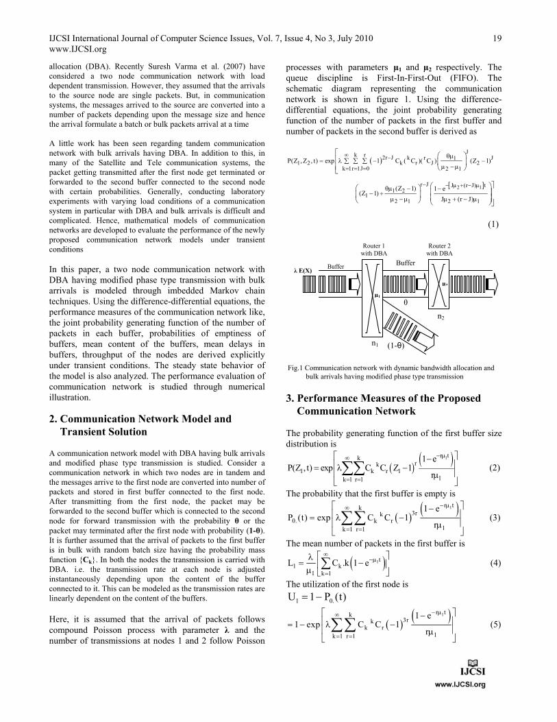
IJCSI International Journal of Computer Science Issues, Vol. 7, Issue 4, No 3, July 2010 www.IJCSI.org
19
allocation (DBA). Recently Suresh Varma et al. (2007) have considered a two node communication network with load dependent transmission. However, they assumed that the arrivals to the source node are single packets. But, in communication systems, the messages arrived to the source are converted into a number of packets depending upon the message size and hence the arrival formulate a batch or bulk packets arrival at a time A little work has been seen regarding tandem communication network with bulk arrivals having DBA. In addition to this, in many of the Satellite and Tele communication systems, the packet getting transmitted after the first node get terminated or forwarded to the second buffer connected to the second node with certain probabilities. Generally, conducting laboratory experiments with varying load conditions of a communication system in particular with DBA and bulk arrivals is difficult and complicated. Hence, mathematical models of communication networks are developed to evaluate the performance of the newly proposed communication network models under transient conditions In this paper, a two node communication network with DBA having modified phase type transmission with bulk arrivals is modeled through imbedded Markov chain techniques. Using the difference-differential equations, the performance measures of the communication network like, the joint probability generating function of the number of packets in each buffer, probabilities of emptiness of buffers, mean content of the buffers, mean delays in buffers, throughput of the nodes are derived explicitly under transient conditions. The steady state behavior of the model is also analyzed. The performance evaluation of communication network is studied through numerical illustration.
2. Communication Network Model and Transient Solution A communication network model with DBA having bulk arrivals and modified phase type transmission is studied. Consider a communication network in which two nodes are in tandem and the messages arrive to the first node are converted into number of packets and stored in first buffer connected to the first node. After transmitting from the first node, the packet may be forwarded to the second buffer which is connected to the second node for forward transmission with the probability θ or the packet may terminated after the first node with probability (1-θ). It is further assumed that the arrival of packets to the first buffer is in bulk with random batch size having the probability mass function {Ck}. In both the nodes the transmission is carried with DBA. i.e. the transmission rate at each node is adjusted instantaneously depending upon the content of the buffer connected to it. This can be modeled as the transmission rates are linearly dependent on the content of the buffers. Here, it is assumed that the arrival of packets follows compound Poisson process with parameter λ and the number of transmissions at nodes 1 and 2 follow Poisson
processes with parameters µ1 and µ2 respectively. The queue discipline is First-In-First-Out (FIFO). The schematic diagram representing the communication network is shown in figure 1. Using the difference-differential equations, the joint probability generating function of the number of packets in the first buffer and number of packets in the second buffer is derived as
2 1
Jk r 2r J k r J11 2 k r J 2
k 1r 1J 0 2 1
r J J (r J) t1 2
12 1 2 1
P(Z , Z , t) exp 1 C ( C )( C ) (Z 1)
(Z 1) 1 e(Z 1)
J (r J)
(1)
Fig.1 Communication network with dynamic bandwidth allocation and bulk arrivals having modified phase type transmission
3. Performance Measures of the Proposed Communication Network The probability generating function of the first buffer size distribution is
1r tk
rk1 k r 1
1k 1 r 1
1 eP(Z , t) exp C C Z 1
r
(2)
The probability that the first buffer is empty is
1r tk
3rk0. k r
1k 1 r 1
1 eP (t) exp C C 1
r
(3)
The mean number of packets in the first buffer is
1t1 k
1 k 1
L C .k 1 e
(4)
The utilization of the first node is
)t(P1U .01
1r tk
3rkk r
1k 1 r 1
1 e1 exp C C 1
r
(5)
Router 1 with DBA
Router 2 with DBA
Buffer Buffer λ E(X)
θ
(1-θ)
μ1
μ2
n2
n1
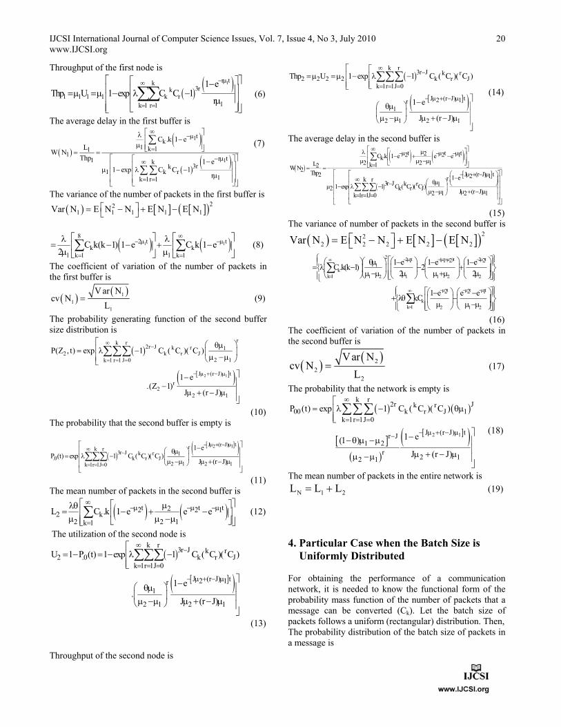
IJCSI International Journal of Computer Science Issues, Vol. 7, Issue 4, No 3, July 2010 www.IJCSI.org
20
Throughput of the first node is
1r tk
3rk1 1 1 1 k r
1k 1 r 1
1 eThp U 1 exp C C 1
r
(6)
The average delay in the first buffer is
1
1
tk
1 k 111
r t1 k3rk
1 k r1k 1r 1
C .k 1 eL
W NThp 1 e
1 exp C C 1r
(7)
The variance of the number of packets in the first buffer is
221 1 1 1 1Var N E N N E N E N
1 1
82 t t
k k1 1k 1 k 1
C k(k 1) 1 e C k 1 e2
(8)
The coefficient of variation of the number of packets in the first buffer is
1
11
V ar Ncv N
L (9)
The probability generating function of the second buffer size distribution is
2 1
rk r2r J k r 1
2 k r J2 1k 1 r 1 J 0
J (r J) t
r2
2 1
P(Z , t) exp 1 C ( C )( C )
1 e.(Z 1)
J (r J)
(10) The probability that the second buffer is empty is
2 1J (r J) trk r
3r J k r 1.0 k r J
2 1 2 1k 1r 1J 0
1 eP (t) exp 1 C ( C )( C )
J (r J)
(11) The mean number of packets in the second buffer is
t t t22 2 12 k
2 2 1k 1
L C .k 1 e e e
(12)
The utilization of the second node is
k r3r J k r
2 .0 k r Jk 1r 1J 0
J (r J) t2 1r1
2 1 2 1
U 1 P (t) 1 exp 1 C ( C )( C )
1 e.
J (r J)
(13) Throughput of the second node is
k r3r J k r
2 2 2 2 k r Jk 1r 1J 0
J (r J) t2 1r1
2 1 2 1
Thp U 1 exp 1 C ( C )( C )
1 e
J (r J)
(14)
The average delay in the second buffer is
t t t22 2 1C .k 1 e e ek2 2 1L k 12W N2 Thp J (r J) t2 2 11 erk r
3r J k r 11 exp 1 C ( C )( C )2 k r J J (r J)2 1 2 1k 1r 1J 0
(15) The variance of number of packets in the second buffer is
222 2 2 2 2Var N E N N E N E N
2 2 t ( )t 2 t1
kk 1 1 2 1 1 2 2
t t t
kk 1 2 1 2
1 1 2 2
2 2 1
1 e 1 e 1 eC.k(k 1) 2
2 2
1 e e ek.C
(16) The coefficient of variation of the number of packets in the second buffer is
22
2
Var Ncv N
L (17)
The probability that the network is empty is
2 1
k r2r Jk r
00 k r J 1k 1r 1J 0
J (r J) tr J1 2
r2 12 1
P (t) exp 1 C ( C )( C )
1 e(1 )
J (r J)
(18)
The mean number of packets in the entire network is
N 1 2L L L (19)
4. Particular Case when the Batch Size is Uniformly Distributed For obtaining the performance of a communication network, it is needed to know the functional form of the probability mass function of the number of packets that a message can be converted (Ck). Let the batch size of packets follows a uniform (rectangular) distribution. Then, The probability distribution of the batch size of packets in a message is

IJCSI International Journal of Computer Science Issues, Vol. 7, Issue 4, No 3, July 2010 www.IJCSI.org
21
k
1C
b a 1
for k=a, a+1,…, b.
The mean number of packets in a message is
a b
2
and its variance is 21b a 1 1
12 .
Substituting the value of Ck in Eq. (1), we get the joint probability generating function of the number of packets in both the buffers is
2 1
Jb k r2r J k r J1
1 2 r J 22 1k ar 1J 0
J (r J) tr J1 2
12 1 2 1
1P(Z ,Z ,t) exp 1 ( C )( C ) (Z 1)
b a 1
1 e(Z 1)
(Z 1)J (r J)
(20) The probability generating function of the first buffer size distribution is
1r tb k
rk1 r 1
1k a r 1
1 e1P(Z ,t) exp C Z 1
b a 1 r
(21)
The probability that the first buffer is empty is
1r tb k
3rk0. r
1k a r 1
1 e1P (t) exp C 1
b a 1 r
(22)
The mean number of packets in the first buffer is
1t1
1
(a b)L 1 e
2
(23)
The utilization of the first node is
1r tb k
3rk1 0. r
1k a r 1
1 e1U 1 P (t) 1 exp C 1
b a 1 r
(24)
Throughput of the first node is
1r tb k
3rk1 1 1 1 r
1k a r 1
1 e1Thp .U 1 exp C 1
b a 1 r
(25)
The average delay in the first buffer is
1
1
t
1 11
r t1 b k3rk
1 r1k a r 1
(a b)1 e
L 2W N
Thp 1 e11 exp C 1
b a 1 r
(26)
The variance of the number of packets in the first buffer is
221 1 1 1 1Var N E N N E N E N
1 12 t tb b
1 1k a k a
1 1 e 1 1 ek(k 1) k
b a 1 2 b a 1
(27)
The coefficient of variation of the number of packets in the first buffer is
11
1
Var Ncv N
L (28)
The probability generating function of the second buffer size distribution is
2 1
b k r2r J k r
2 r Jk a r 1J 0
J (r J) trr1
22 1 2 1
1P(Z , t) exp 1 ( C )( C )
b a 1
1 e. (Z 1)
J (r J)
(29)
The probability that the second buffer is empty is
2 1
b k r3r J k r
.0 r Jk a r 1J 0
J (r J) tr1
2 1 2 1
1P (t) exp 1 ( C )( C )
b a 1
1 e
J (r J)
(30)
The mean number of packets in the second buffer is
2 2 1t t t22
2 2 1
(a b)L 1 e e e
2
(31)
The utilization of the second node is
2 1
b k r3r J k r
2 .0 r Jk a r 1J 0
J (r J) tr1
2 1 2 1
1U 1 P (t) 1 exp 1 ( C )( C )
b a 1
1 e
J (r J)
(32)
Throughput of the second node is
2 1
b k r3r J k r
2 2 2 2 r Jk a r 1J 0
J (r J) tr1
2 1 2 1
1Thp .U 1 exp 1 ( C )( C )
b a 1
1 e
J (r J)
(33)
The average delay in the second buffer is
22
2
LW N
T h p
2 2 1
2 1
t t t2
2 2 1
J (r J) trb k r3r J k r 1
2 r J2 1 2 1k ar 1J 0
(a b)1 e e e
2
1 e1
1 exp 1 ( C )( C )b a 1 J (r J)
(34)
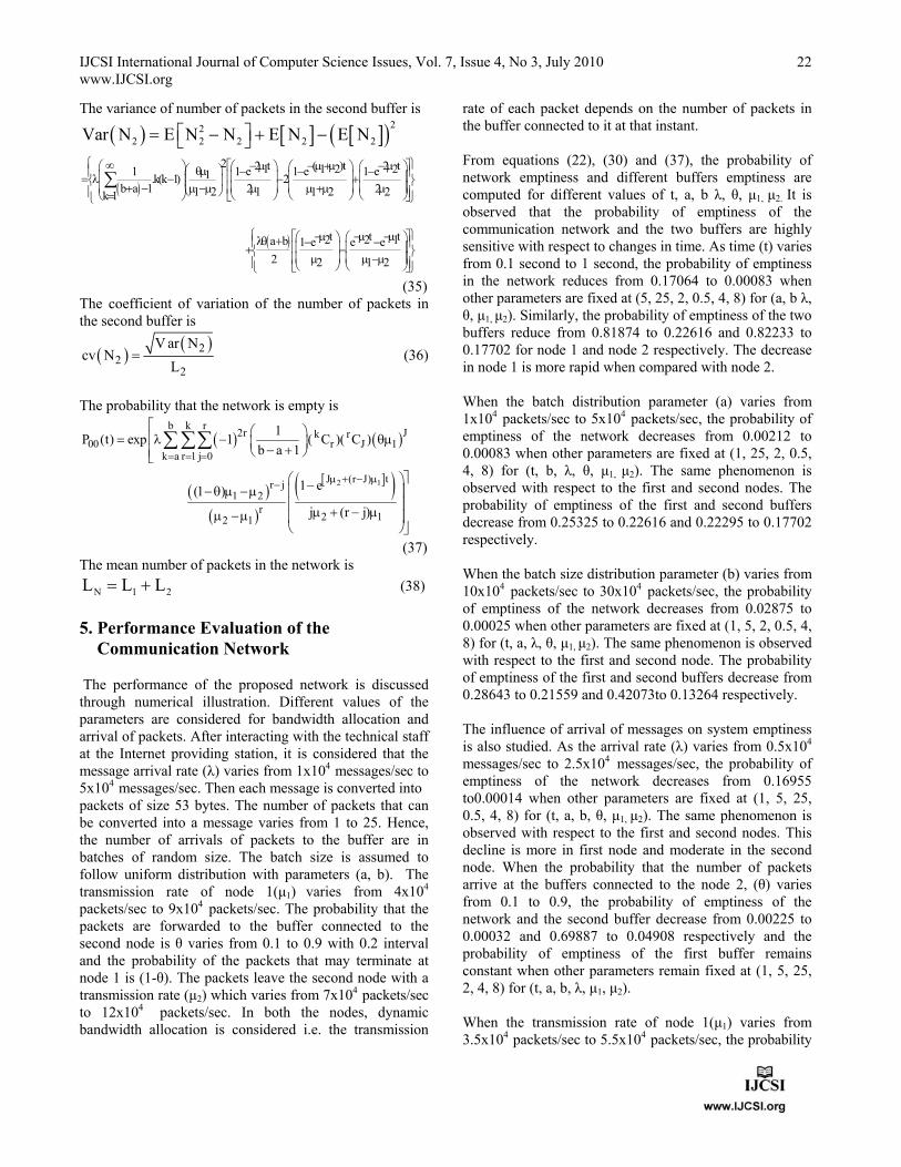
IJCSI International Journal of Computer Science Issues, Vol. 7, Issue 4, No 3, July 2010 www.IJCSI.org
22
The variance of number of packets in the second buffer is
222 2 2 2 2Var N E N N E N E N
2 2 t ( )t 2 t1 1 2 21 1 e 1 e 1 e1.k(k 1) 2b a 1 2 21 2 1 1 2 2k 1
t t t2 2 1a b 1 e e e
2 2 1 2
(35) The coefficient of variation of the number of packets in the second buffer is
2
22
V ar Ncv N
L (36)
The probability that the network is empty is
2 1
b k r2r Jk r
00 r J 1k a r 1 j 0
J (r J) tr j1 2
r2 12 1
1P (t) exp 1 ( C )( C )
b a 1
1 e(1 )
j (r j)
(37) The mean number of packets in the network is
N 1 2L L L (38)
5. Performance Evaluation of the Communication Network The performance of the proposed network is discussed through numerical illustration. Different values of the parameters are considered for bandwidth allocation and arrival of packets. After interacting with the technical staff at the Internet providing station, it is considered that the message arrival rate (λ) varies from 1x10⁴ messages/sec to 5x10⁴ messages/sec. Then each message is converted into packets of size 53 bytes. The number of packets that can be converted into a message varies from 1 to 25. Hence, the number of arrivals of packets to the buffer are in batches of random size. The batch size is assumed to follow uniform distribution with parameters (a, b). The transmission rate of node 1(μ1) varies from 4x10⁴
packets/sec to 9x10⁴ packets/sec. The probability that the packets are forwarded to the buffer connected to the second node is θ varies from 0.1 to 0.9 with 0.2 interval and the probability of the packets that may terminate at node 1 is (1-θ). The packets leave the second node with a transmission rate (μ2) which varies from 7x10⁴ packets/sec to 12x104 packets/sec. In both the nodes, dynamic bandwidth allocation is considered i.e. the transmission
rate of each packet depends on the number of packets in the buffer connected to it at that instant. From equations (22), (30) and (37), the probability of network emptiness and different buffers emptiness are computed for different values of t, a, b λ, θ, μ1, μ2. It is observed that the probability of emptiness of the communication network and the two buffers are highly sensitive with respect to changes in time. As time (t) varies from 0.1 second to 1 second, the probability of emptiness in the network reduces from 0.17064 to 0.00083 when other parameters are fixed at (5, 25, 2, 0.5, 4, 8) for (a, b λ, θ, μ1, μ2). Similarly, the probability of emptiness of the two buffers reduce from 0.81874 to 0.22616 and 0.82233 to 0.17702 for node 1 and node 2 respectively. The decrease in node 1 is more rapid when compared with node 2. When the batch distribution parameter (a) varies from 1x10⁴ packets/sec to 5x10⁴ packets/sec, the probability of emptiness of the network decreases from 0.00212 to 0.00083 when other parameters are fixed at (1, 25, 2, 0.5, 4, 8) for (t, b, λ, θ, μ1, μ2). The same phenomenon is observed with respect to the first and second nodes. The probability of emptiness of the first and second buffers decrease from 0.25325 to 0.22616 and 0.22295 to 0.17702 respectively. When the batch size distribution parameter (b) varies from 10x104 packets/sec to 30x104 packets/sec, the probability of emptiness of the network decreases from 0.02875 to 0.00025 when other parameters are fixed at (1, 5, 2, 0.5, 4, 8) for (t, a, λ, θ, μ1, μ2). The same phenomenon is observed with respect to the first and second node. The probability of emptiness of the first and second buffers decrease from 0.28643 to 0.21559 and 0.42073to 0.13264 respectively. The influence of arrival of messages on system emptiness is also studied. As the arrival rate (λ) varies from 0.5x10⁴
messages/sec to 2.5x10⁴ messages/sec, the probability of emptiness of the network decreases from 0.16955 to0.00014 when other parameters are fixed at (1, 5, 25, 0.5, 4, 8) for (t, a, b, θ, μ1, μ2). The same phenomenon is observed with respect to the first and second nodes. This decline is more in first node and moderate in the second node. When the probability that the number of packets arrive at the buffers connected to the node 2, (θ) varies from 0.1 to 0.9, the probability of emptiness of the network and the second buffer decrease from 0.00225 to 0.00032 and 0.69887 to 0.04908 respectively and the probability of emptiness of the first buffer remains constant when other parameters remain fixed at (1, 5, 25, 2, 4, 8) for (t, a, b, λ, μ1, μ2). When the transmission rate of node 1(μ1) varies from 3.5x10⁴ packets/sec to 5.5x10⁴ packets/sec, the probability

IJCSI International Journal of Computer Science Issues, Vol. 7, Issue 4, No 3, July 2010 www.IJCSI.org
23
of emptiness of the network and the first buffer increase from 0.00042 to 0.00347 and 0.19894 to 0.31598 respectively and the probability of emptiness of the second buffer decreases from 0.18161 to 0.17202 when other parameters remain fixed at (1, 5, 25, 2, 0.5, 8) for (t, a, b, λ, θ, μ2). When the transmission rate of node 2 (μ2) varies from 6x10⁴ packets/sec to 10x104 packets/sec, the probability of emptiness of the network and the second buffer increase from 0.00054 to 0.00107 and 0.10484 to 0.24604 respectively when other parameters remain fixed at (1, 5, 25, 2, 0.5, 4) for (t, a, b, λ, θ, μ1).. From the equations (23), (24), (31), (32) and (38), the mean number of packets and the utilization of the network are computed for different values of t, a, b, λ, θ, μ1, μ2. The values for mean number of packets in the two buffers and mean delays are given in Table.1 and the relationship between mean number of packets in the two buffers and the input parameters t, a, b, λ, θ, μ1, μ2 is shown in Figures 2, 3, 4 and 5.
Table 1: Values of mean number packets and mean delays in the two buffers
t* a b λ# θ μ1
$ μ2$ L1 L2 W(N1) W(N2)
0.1 0.3 0.5 0.8 1.0
1 1 1 1 1
5 5 5 5 5
3 3 3 3 3
0.5 0.5 0.5 0.5 0.5
4 4 4 4 4
7 7 7 7 7
0.74178 1.57231 1.94550 2.15829 2.20879
0.06302 0.29603 0.46574 0.58488 0.61617
0.74500 0.74856 0.75803 0.76697 0.76955
0.15320 0.17318 0.18615 0.19518 0.19756
1 1 1 1 1
1 2 3 4 5
25 25 25 25 25
2 2 2 2 2
0.5 0.5 0.5 0.5 0.5
4 4 4 4 4
8 8 8 8 8
6.38095 6.62637 6.97179 7.11721 7.36263
1.56602 1.62625 1.68648 1.74671 1.80695
2.13623 2.19156 2.25159 2.31425 2.37859
0.25192 0.25748 0.26308 0.26874 0.27445
1 1 1 1 1
5 5 5 5 5
10 15 20 25 30
2 2 2 2 2
0.5 0.5 0.5 0.5 0.5
4 4 4 4 4
8 8 8 8 8
3.68132 4.90842 6.13553 7.36263 8.58974
0.90347 1.20463 1.50579 1.80695 2.10810
1.28975 1.65526 2.01797 2.37859 2.73766
0.19496 0.21991 0.24644 0.27445 0.30381
1 1 1 1 1
5 5 5 5 5
25 25 25 25 25
0.5 1.0 1.5 2.0 2.5
0.5 0.5 0.5 0.5 0.5
4 4 4 4 4
8 8 8 8 8
1.84066 3.68132 5.52197 7.36263 9.20329
0.45174 0.90347 1.35521 1.80695 2.25868
1.48252 1.75487 2.05415 2.37859 2.72596
0.16071 0.19496 0.23298 0.27445 0.31896
1 1 1 1 1
5 5 5 5 5
25 25 25 25 25
2 2 2 2 2
0.1 0.3 0.5 0.7 0.9
4 4 4 4 4
8 8 8 8 8
7.36263 7.36263 7.36263 7.36263 7.36263
0.36139 1.08417 1.80695 2.52972 3.25250
2.37859 2.37859 2.37859 2.37859 2.37859
0.15001 0.20773 0.27445 0.34833 0.42755
1 1 1 1 1
5 5 5 5 5
25 25 25 25 25
2 2 2 2 2
0.5 0.5 0.5 0.5 0.5
2.5 3.0 3.5 4.0 4.5
8 8 8 8 8
11.01498 9.50213 8.31259 7.36263 6.59261
1.65142 1.72602 1.77483 1.80695 1.82820
5.22978 3.84195 2.96485 2.37859 1.96811
0.25878 0.26613 0.27108 0.27445 0.27677
1 1 1 1 1
5 5 5 5 5
25 25 25 25 25
2 2 2 2 2
0.5 0.5 0.5 0.5 0.5
4 4 4 4 4
5 6 7 8 9
7.36263 7.36263 7.36263 7.36263 7.36263
2.80612 2.37503 2.05388 1.80695 1.61188
2.37859 2.37859 2.37859 2.37859 2.37859
0.60400 0.44220 0.34151 0.27445 0.22737
* = seconds, # =Multiples of 10,000 Messages/sec,
$= Multiples of 10,000 Packets/sec
a Vs Mean number of Packets
0
2
4
6
8
0 1 2 3 4 5 6
a
Mea
n nu
mbe
r of
Pac
kets
L1
L2
Fig. 2 Batch size distribution parameter a Vs Mean
number of Packets in the buffers 1 and 2
0
2
4
6
8
10
0 10 20 30 40
Mea
n nu
mbe
r of
Pac
kets
b
b Vs Mean number of Packets
L1
L2
Fig. 3 Batch size distribution parameter b Vs Mean
number of Packets in the buffers 1 and 2
00.40.81.21.6
22.42.8
0 1 2 3 4 5 6
Mea
n D
elay
a
a Vs Mean Delay
W(N1)
W(N2)
Fig. 4 Batch size distribution parameter a Vs Mean
delay in the buffers 1 and 2
0
0.5
1
1.5
2
2.5
3
0 5 10 15 20 25 30 35
Mea
n D
eala
y
b
b Vs Mean Delay
W(N1)
W(N2)
Fig. 5 Batch size distribution parameter b Vs Mean delay in the buffers 1 and 2
It is observed that after 0.1 seconds, the first buffer is having on an average of 7417.8 packets, after 0.3 seconds it rapidly raised to an average of 15723.1 packets. After 1 second, the first buffer is containing an average of
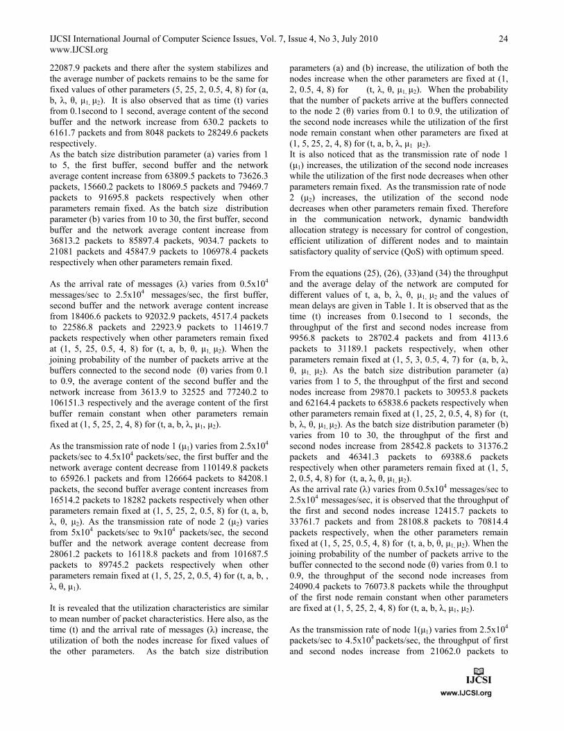
IJCSI International Journal of Computer Science Issues, Vol. 7, Issue 4, No 3, July 2010 www.IJCSI.org
24
22087.9 packets and there after the system stabilizes and the average number of packets remains to be the same for fixed values of other parameters (5, 25, 2, 0.5, 4, 8) for (a, b, λ, θ, μ1, μ2). It is also observed that as time (t) varies from 0.1second to 1 second, average content of the second buffer and the network increase from 630.2 packets to 6161.7 packets and from 8048 packets to 28249.6 packets respectively. As the batch size distribution parameter (a) varies from 1 to 5, the first buffer, second buffer and the network average content increase from 63809.5 packets to 73626.3 packets, 15660.2 packets to 18069.5 packets and 79469.7 packets to 91695.8 packets respectively when other parameters remain fixed. As the batch size distribution parameter (b) varies from 10 to 30, the first buffer, second buffer and the network average content increase from 36813.2 packets to 85897.4 packets, 9034.7 packets to 21081 packets and 45847.9 packets to 106978.4 packets respectively when other parameters remain fixed. As the arrival rate of messages (λ) varies from 0.5x10⁴
messages/sec to 2.5x10⁴ messages/sec, the first buffer, second buffer and the network average content increase from 18406.6 packets to 92032.9 packets, 4517.4 packets to 22586.8 packets and 22923.9 packets to 114619.7 packets respectively when other parameters remain fixed at (1, 5, 25, 0.5, 4, 8) for (t, a, b, θ, μ1, μ2). When the joining probability of the number of packets arrive at the buffers connected to the second node (θ) varies from 0.1 to 0.9, the average content of the second buffer and the network increase from 3613.9 to 32525 and 77240.2 to 106151.3 respectively and the average content of the first buffer remain constant when other parameters remain fixed at (1, 5, 25, 2, 4, 8) for (t, a, b, λ, μ1, μ2). As the transmission rate of node 1 (μ1) varies from 2.5x10⁴
packets/sec to 4.5x10⁴ packets/sec, the first buffer and the network average content decrease from 110149.8 packets to 65926.1 packets and from 126664 packets to 84208.1 packets, the second buffer average content increases from 16514.2 packets to 18282 packets respectively when other parameters remain fixed at (1, 5, 25, 2, 0.5, 8) for (t, a, b, λ, θ, μ2). As the transmission rate of node 2 (μ2) varies from 5x10⁴ packets/sec to 9x10⁴ packets/sec, the second buffer and the network average content decrease from 28061.2 packets to 16118.8 packets and from 101687.5 packets to 89745.2 packets respectively when other parameters remain fixed at (1, 5, 25, 2, 0.5, 4) for (t, a, b, , λ, θ, μ1). It is revealed that the utilization characteristics are similar to mean number of packet characteristics. Here also, as the time (t) and the arrival rate of messages (λ) increase, the utilization of both the nodes increase for fixed values of the other parameters. As the batch size distribution
parameters (a) and (b) increase, the utilization of both the nodes increase when the other parameters are fixed at (1, 2, 0.5, 4, 8) for (t, λ, θ, μ1, μ2). When the probability that the number of packets arrive at the buffers connected to the node 2 (θ) varies from 0.1 to 0.9, the utilization of the second node increases while the utilization of the first node remain constant when other parameters are fixed at (1, 5, 25, 2, 4, 8) for (t, a, b, λ, μ1 μ2). It is also noticed that as the transmission rate of node 1 (μ1) increases, the utilization of the second node increases while the utilization of the first node decreases when other parameters remain fixed. As the transmission rate of node 2 (μ2) increases, the utilization of the second node decreases when other parameters remain fixed. Therefore in the communication network, dynamic bandwidth allocation strategy is necessary for control of congestion, efficient utilization of different nodes and to maintain satisfactory quality of service (QoS) with optimum speed. From the equations (25), (26), (33)and (34) the throughput and the average delay of the network are computed for different values of t, a, b, λ, θ, μ1, μ2 and the values of mean delays are given in Table 1. It is observed that as the time (t) increases from 0.1second to 1 seconds, the throughput of the first and second nodes increase from 9956.8 packets to 28702.4 packets and from 4113.6 packets to 31189.1 packets respectively, when other parameters remain fixed at (1, 5, 3, 0.5, 4, 7) for (a, b, λ, θ, μ1, μ2). As the batch size distribution parameter (a) varies from 1 to 5, the throughput of the first and second nodes increase from 29870.1 packets to 30953.8 packets and 62164.4 packets to 65838.6 packets respectively when other parameters remain fixed at (1, 25, 2, 0.5, 4, 8) for (t, b, λ, θ, μ1, μ2). As the batch size distribution parameter (b) varies from 10 to 30, the throughput of the first and second nodes increase from 28542.8 packets to 31376.2 packets and 46341.3 packets to 69388.6 packets respectively when other parameters remain fixed at (1, 5, 2, 0.5, 4, 8) for (t, a, λ, θ, μ1, μ2). As the arrival rate (λ) varies from 0.5x10⁴ messages/sec to 2.5x10⁴ messages/sec, it is observed that the throughput of the first and second nodes increase 12415.7 packets to 33761.7 packets and from 28108.8 packets to 70814.4 packets respectively, when the other parameters remain fixed at (1, 5, 25, 0.5, 4, 8) for (t, a, b, θ, μ1, μ2). When the joining probability of the number of packets arrive to the buffer connected to the second node (θ) varies from 0.1 to 0.9, the throughput of the second node increases from 24090.4 packets to 76073.8 packets while the throughput of the first node remain constant when other parameters are fixed at (1, 5, 25, 2, 4, 8) for (t, a, b, λ, μ1, μ2). As the transmission rate of node 1(μ1) varies from 2.5x10⁴
packets/sec to 4.5x10⁴ packets/sec, the throughput of first and second nodes increase from 21062.0 packets to
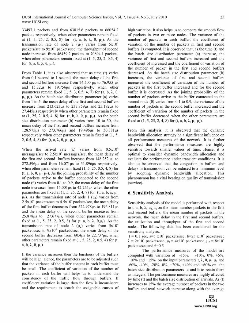
IJCSI International Journal of Computer Science Issues, Vol. 7, Issue 4, No 3, July 2010 www.IJCSI.org
25
33497.1 packets and from 63815.6 packets to 66054.2 packets respectively, when other parameters remain fixed at (1, 5, 25, 2, 0.5, 8) for (t, a, b, λ, θ, μ2). As the transmission rate of node 2 (μ2) varies from 5x10⁴
packets/sec to 9x10⁴ packets/sec, the throughput of second node increases from 46459.2 packets to 70894.1 packets, when other parameters remain fixed at (1, 5, 25, 2, 0.5, 4) for (t, a, b, λ, θ, μ1). From Table 1, it is also observed that as time (t) varies from 0.1 second to 1 second, the mean delay of the first and second buffers increase from 74.500 μs to 76.955 μs and 15.32μs to 19.756μs respectively, when other parameters remain fixed (1, 5, 3, 0.5, 4, 7) for (a, b, λ, θ, μ1, μ2). As the batch size distribution parameter (a) varies from 1 to 5, the mean delay of the first and second buffers increase from 213.623μs to 237.859μs and 25.192μs to 27.445μs respectively when other parameters remain fixed at (1, 25, 2, 0.5, 4, 8) for (t, b, λ, θ, μ1, μ2). As the batch size distribution parameter (b) varies from 10 to 30, the mean delay of the first and second buffers increase from 128.975μs to 273.766μs and 19.496μs to 30.381μs respectively when other parameters remain fixed at (1, 5, 2, 0.5, 4, 8) for (t, a, λ, θ, μ1, μ2). When the arrival rate (λ) varies from 0.5x10⁴
messages/sec to 2.5x10⁴ messages/sec, the mean delay of the first and second buffers increase from 148.252μs to 272.596μs and from 16.071μs to 31.896μs respectively, when other parameters remain fixed (1, 5, 25, 0.5, 4, 8) for (t, a, b, θ, μ1, μ2). As the joining probability of the number of packets arrive to the buffer connected to the second node (θ) varies from 0.1 to 0.9, the mean delay of the first node increases from 15.001μs to 42.755μs when the other parameters are fixed at (1, 5, 25, 2, 4, 8) for (t, a, b, λ, μ1,
μ2). As the transmission rate of node 1 (μ1) varies from 2.5x10⁴ packets/sec to 4.5x10⁴ packets/sec, the mean delay of the first buffer decreases from 522.978μs to 196.811μs and the mean delay of the second buffer increases from 25.878μs to 27.677μs, when other parameters remain fixed at (1, 5, 25, 2, 0.5, 8) for (t, a, b, λ, θ,μ2). As the transmission rate of node 2 (μ2) varies from 5x10⁴
packets/sec to 9x10⁴ packets/sec, the mean delay of the second buffer decreases from 60.4μs to 22.737μs, when other parameters remain fixed at (1, 5, 25, 2, 0.5, 4) for (t, a, b, λ, θ, μ1). If the variance increases then the burstness of the buffers will be high. Hence, the parameters are to be adjusted such that the variance of the buffer content in each buffer must be small. The coefficient of variation of the number of packets in each buffer will helps us to understand the consistency of the traffic flow through buffers. If coefficient variation is large then the flow is inconsistent and the requirement to search the assignable causes of
high variation. It also helps us to compare the smooth flow of packets in two or more nodes. The variance of the number of packets in each buffer, the coefficient of variation of the number of packets in first and second buffers is computed. It is observed that, as the time (t) and the batch size distribution parameter (a) increase, the variance of first and second buffers increased and the coefficient of increased and the coefficient of variation of the number of packet in the first and second buffers decreased. As the batch size distribution parameter (b) increases, the variance of first and second buffers increased the coefficient of variation of the number of packets in the first buffer increased and for the second buffer it is decreased. As the joining probability of the number of packets arrive to the buffer connected to the second node (θ) varies from 0.1 to 0.9, the variance of the number of packets in the second buffer increased and the coefficient of variation of the number of packets in the second buffer decreased when the other parameters are fixed at (1, 5, 25, 2, 4, 8) for (t, a, b, λ, μ1, μ2). From this analysis, it is observed that the dynamic bandwidth allocation strategy ha a significant influence on all performance measures of the network. It is further observed that the performance measures are highly sensitive towards smaller values of time. Hence, it is optimal to consider dynamic bandwidth allocation and evaluate the performance under transient conditions. It is also to be observed that the congestion in buffers and delays in transmission can be reduced to a minimum level by adopting dynamic bandwidth allocation. This phenomenon has a vital bearing on quality of transmission (service). 6. Sensitivity Analysis Sensitivity analysis of the model is performed with respect to t, a, b, λ, μ1, μ2 on the mean number packets in the first and second buffers, the mean number of packets in the network, the mean delay in the first and second buffers, the utilization and throughput of the first and second nodes. The following data has been considered for the sensitivity analysis. t = 0.1 sec, a=5 x10⁴ packets/sec, b=25 x104 packets/sec λ = 2x10⁴ packets/sec, μ1 = 4x10⁴ packets/sec, μ2 = 8x10⁴
packets/sec and θ=0.5 The performance measures of the model are computed with variation of -15%, -10%, 0%, +5%, +10% and +15% on the input parameters t, λ, θ, μ1, μ2 and -60%, -40%, -20%, 0%, +20%, +40% and +60% on the batch size distribution parameters a and b to retain them as integers. The performance measures are highly affected by time (t) and the batch size distribution of arrivals. As (t) increases to 15% the average number of packets in the two buffers and total network increase along with the average
IJCSI International Journal of Computer Science Issues, Vol. 7, Issue 4, No 3, July 2010 www.IJCSI.org
26
delays in buffers. Similarly, as arrival rate of messages (λ) increases by 15% the average number of packets in the two buffers and total network increases along with the average delays in buffers. The mean delays and mean content of the buffers are decreasing function of these parameters. Overall analysis of the parameters reflects that dynamic bandwidth allocation strategy for congestion control tremendously reduces the delays in communication and improves voice quality by reducing burstness in buffers. 7. Conclusions In this paper, a two node tandem communication network with dynamic bandwidth allocation having bulk arrivals and modified phase type transmission is developed and analyzed. Here, the dynamic bandwidth allocation (DBA) strategy insists for the instantaneous change in rate of transmission of the nodes depending upon the content of the buffers connected to them. The emphasis of this communication network is on the bulk or batch arrivals of packets to the initial node with random size. The performance of the statistical multiplexing is measured by approximating the arrival process with a compound Poisson process and the transmission process with Poisson process. This is chosen such that the statistical characteristics of the communication network identically matches with Poisson process and uniform distribution. A communication network model with modified phase type transmission is more close to the practical transmission behavior in most of the communication systems. The sensitivity of the network with respect to input parameters is studied through numerical illustrations. It is observed that the dynamic bandwidth allocation strategy and the parameters of bulk size distribution have a significant impact on the performance measures of the network. It is further observed that transient analysis of the Communication network will approximate the performance measures more close to the practical situation. This network can also be extended to the multi node communication networks. It is interesting to note that this Communication network model includes some of the earlier Communication network model given by P.S.Varma and K.Srinivasa Rao (2007) References [1]. K. Srinivasa Rao, Prasad Reddy and P. SureshVarma
(2006). Inter dependent communication network with bulk arrivals, International Journal of Management and Systems, Vol.22, No.3, pp. 221-234
[2]. Kin K. Leung (2002), Load dependent service queues with application to congestion control in broadband networks, Performance Evaluation, Vol.50, Issue 1-4, pp 27-40.
[3]. Karanam, V.R, Sriram, K. and Boiwkere D.O (1988). Performance evaluation of variable bit rate voice in packet
– switched networks, AT&T Technical Journal, pp. 41-56 and Proc. GLOBECOM’88, Hollywood, Florida, pp. 1617- 1622.
[4]. Emre Yetginer and Ezhan Karasan (2008), dynamic wavelength allocation in IP/WDM metro access networks, IEEE Journal on selected areas in Communications, Vol.26, No.3, pp 13-27.
[5]. Gunadle, A.S and Yadri, A.R (2008), Performance evaluation of issues related to video over broadband networks, Proceedings of World Academy of Sciences, Engineering and technology, Vol.36, pp 122-125
[6]. Hongwang Yu and yufan Zheng (2009), Global behavior of dynamical agents in direct network, Journal of control theory and applications, Vol.7, No.3, pp 307-314.
[7]. Fen Zhou, Miklos Molnar and Bernard Cousin (2009), Avoidance of multicast incapable branching nodes for multicast routing in WDM, Photonic network communications, Vol.18, No.3, pp378-392.
[8]. Stanislav Angelov, Sanjeev Khanna and Keshav Kunal (2009), The network as a storage device:Dynamic routing with bounded buffers, Algorithmica, Vol.55, No.1, pp 71-94.
[9]. P.Suresh Varma and K.Srinivasa Rao (2007), A Communication network with load dependent transmission, International Journal of Matnemetical Sciences, Vol.6, No.2, pp 199-210.
Mr. Kuda. Nageswara Rao is presently working as Associate professor in the Department of Computer Science and Systems Engineering, Andhra University, Visakhapatnam. He presented several research papers in national and International conferences and seminars. He published a good number of papers in national and International journals. He guided several students for getting their M.Tech degrees in Computer Science and Engineering. His current research interests are Communication networks, Internet Technologies and Network security. Dr. K.Srinivasa Rao is presently working as Professor and head, Department of Statistics, Andhra University, Visakhapatnam. He is elected chief editor of Journal of ISPS and elected Vice-President of Operation Research of India. He guided 22 students for Ph.D in Statistics, Computer Science, Electronics and Communications and Operations Research. He published 75 research papers in national and International journals with high reputation. His research interests are Communication Systems, Data Mining and stochastic models. Dr. Peri. Srinivasa Rao is presently working as Professor in the Department of Computer Science and Systems Engineering, Andhra University, Visakhapatnam. He got his Ph.D degree from Indian Institute of Technology, Kharagpur in Computer Science in 1987. He published several research papers and delivered invited lectures at various conferences, seminars and workshops. He guided a large number of students for their M.Tech degrees in Computer Science and Engineering and Information Technology. His current research interests are Communication networks, Data Mining and Computer Morphology.
IJCSI International Journal of Computer Science Issues, Vol. 7, Issue 4, No 3, July 2010 ISSN (Online): 1694-0784 ISSN (Print): 1694-0814
27
Integrated Machine Learning Techniques for Arabic Named Entity Recognition
Samir AbdelRahman, Mohamed Elarnaoty, Marwa Magdy and Aly Fahmy
Computer Science Department Faculty of Computers and Information, Cairo University
5 Dr. Ahmed Zewail Street, Postal Code: 12613, Orman, Giza, Egypt
Abstract
Named Entity Recognition (NER) task has become essential to improve the performance of many NLP tasks. Its aim is to endeavor a solution to boost accurately the identification of extracted named entities. This paper presents a novel solution for Arabic Named Entity Recognition (ANER) problem. The solution is an integration approach between two machine learning techniques, namely bootstrapping semi-supervised pattern recognition and Conditional Random Fields (CRF) classifier as a supervised technique. The paper solution contributions are the exploit of pattern and word semantic fields as CRF features, the adventure of utilizing bootstrapping semi-supervised pattern recognition technique in Arabic Language, and the integration success to improve the performance of its components. Moreover, as per to our knowledge, this proposed integration has not been utilized for NER task of other natural languages. Using 6-fold cross-validation experimental tests, the solution is proved that it outperforms previous CRF sole work and LingPipe tool. Keywords: Bootstrapping Pattern Recognition, Conditional Random Fields, Arabic Named Recognition, Cross-Validation.
1. Introduction
Named Entity Recognition (NER) is an information extraction subtask to classify proper names from unstructured texts into categories of names. NER task has been used to evolve many Natural Language Processing (NLP) subtasks, such as Information Retrieval and Question Answering [1, 5]. In the last few decades, Arabic Named Entity Recognition (ANER) task has been garnered much efforts to boost its performance. The ANER challenging task is to gather huge corpora or immense white lists/gazetteers that deal with possibly most of Arabic language challenges such as orthography, ambiguity, and complexity. Indeed, most ANER researches tend to collect such data carefully to
include all possible language cases having these peculiarities; though, this data may not exist; the task may not be accurate and it is time-consuming. Consequently, some researchers prefer to use small data set coupled with some tools to help them encounter these problems. We decided to follow this approach and we used the Research and Development International (RDI)1 toolkit to assist us to deal with such difficulties. Many ANER researches have been prompted to use rule-based technique [1, 9, 18, 20] or machine translation techniques [12, 13, 19]. However, their authors state that the proposed systems work effectively if abundant large size corpora for ANER analysis and training phases exist. In the last decade, many machine learning techniques [4, 5, 6] have been exploited using only a set of some language features coupled with small training data sets to build accurate ANER models. Four main points may be concluded from these models. First, the model may lose the identification of some named entities due to the selected features and the small size of such corpora. Second, Conditional Random Fields (CRF) is proved to be one of the most effective learners for ANER task. Third, many Arabic language features have been probed for supervised learning techniques; nevertheless, Arabic semantic fields feature has not been yet considered. Fourth, up to our knowledge, bootstrapping semi-supervised pattern recognition [7] has not been tested as an ANER technique. We present an integration between machine learning techniques to tackle ANER problem for identifying 10 Named Entity (NE) classes namely Person, Location, Organization, Job, Device, Car, Cell Phone, Currency, Date, and Time classes. The proposed integration components are a bootstrapping semi-supervised pattern recognizer and CRF as a supervised learner. This
1 http://www.rdi-eg.com/.

IJCSI International Journal of Computer Science Issues, Vol. 7, Issue 4, No 3, July 2010 www.IJCSI.org
28
integration is novel since to date, up to our knowledge, it has not been utilized in any natural language NER task. The contributions of the proposed solution for ANER task are as follows: 1- We show evidence that bootstrapping semi-supervised pattern recognition technique is a promising ANER technique. 2- We prove that semantic fields feature is one of the effective CRF features. 3- In our approach, both integration components boost iteratively each other. While, the pattern recognizer extracts all expected patterns to let CRF identify more named entities, CRF is trained to employ some local optimal features, including pattern index and word semantic fields, with the aim of generating potential seeds to help in removing the recognizer noisy patterns. To evaluate the first system contribution, we test the resultant patterns manually and we measure their effectiveness to boost CRF in the proposed integration. Moreover, the other two contributions are verified against previous CRF solo work [5] and LingPipe2 tool. The paper is organized as follows: Section 2 illustrates primary Arabic Language challenges; Section 3 explains the thoughts of some related systems; Section 4 presents our approach main three components; Section 5 pinpoints our approach specifications and parameters; Section 6 illustrates how to integrate our solution components; Section 7 submits the experimental results and analysis. Finally, Section 8 draws our conclusions and future work.
2. Arabic Language Challenges
Arabic language is a high complex language which embeds five critical challenges for NLP tasks. First, Arabic is not a case-sensitive language; it has no capital letters. Latin languages consider this feature very significant in NER tasks since their NEs usually start with capital letters. Second, Arabic is a high inflectional language; often a single word has more than one affix such that it may be expressed as a combination of prefix(s), lemma, and suffix(s). The prefixes are articles, prepositions, or conjunctions. The suffixes are generally objects or personal/possessive anaphora. For example, the Arabic word “وبمصريتنا” is interpreted in English as “and that we are Egyptians”.
2Alias-i vendor publishes the LingPipe ANER performance on all 6-fold experiments of the corpus used in this research: http://alias-i.com/lingpipe/demos/tutorial/ne/read-me.html.
Third, Arabic has some variants in spelling and typographic forms. Other languages, such as English, normalize all such variants. For example, “ رامج-غرام ”/ “Gram” 3 is a spelling deviation and “ استراليا-أستراليا ”/ “Australia” is a typographic variant. Fourth, Arabic texts have different sorts of ambiguities (different meanings). For example, “رجب”/“Ragab” in Arabic may be used as a person name, month, or a fear verb. Fifth, Arabic resources, such as corpora, gazetteers, and NLP tools, are either rare or not free. This defect makes collecting and analyzing such resources time-consuming particularly if the NER technique depends on such resources [12, 13, 19, 20].
3. Related work
As a typical supervised learning system, [5] used their owned tagged corpus named ANERcorp4 and gazetteers, ANERGazet, to identify Person, Location, Organization, and Miscellaneous classes with F-measure (Equation 4) of 73.34%, 89.74%, 65.76%, and 61.47% respectively. They prove that CRF precede their ME (Maximum Entropy) work [6] by 12 points in the F-measure average of all classes. We compare our work with this CRF work and we use its tagged corpus and gazetteers as a subset of the research data set (Sections 4, 5, and 7). In this research, we propose a local optimal feature set (Section 5) for each NE class; moreover, we intend someday to investigate [4] and/or other intelligent techniques to find out the optimum feature set for each NE class. Indeed, the supervised learning technique is designed to use a set of features and small size of training data to identify possible categories. In spite of the fact that supervised learning technique precision (Equation 2) is relatively high, its recall (Equation 3) is degraded because its training examples and features may not cover some NE occurrences. In this research, we aim to combine Arabic semantic fields and patterns with other CRF features to boost ANER task. This integration is designed to increase the number of correct NEs and hence to improve the CRF recall. To date, no other natural language NER system follows our proposed integration. Indeed, [8, 14, 15, 21] use bootstrapping supervised learning techniques to improve the corpus training classifier with the most reliable examples extracted from unlabeled data set. Interestingly, 3 Throughout the paper, we use “A”/ “E” as a notation to indicate “E” is an English interpretation of “A”. 4 http://users.dsic.upv.es/~ybenajiba/.

IJCSI International Journal of Computer Science Issues, Vol. 7, Issue 4, No 3, July 2010 www.IJCSI.org
29
[22] and TextRunner 5 present a sort of our proposed integration to serve NE relation extraction task in which the systems are fed with some predefined patterns of relations such that the pattern recognizer and CRF are trained to extract all similar relations and their entities. Even though all mentioned works are sorts of bootstrapping supervised learning, they are not designed for identifying NE classes and their contexts.
4. The Proposed Solution Components
We use Conditional random fields (CRF)6 classifier. It is a discriminative probabilistic model [17] which is used for segmenting and labeling the sequential data. It is a generalization of Hidden Markov Model in which its undirected graph consists of nodes to represent the label sequence y corresponding to the sequence x . The aim of
CRF model is to find y that maximizes )|( xyp
(Equation 1) for that sequence. Section 5.3 describes our proposed CRF feature set.
kk
Yy t kttkk
t kttkk
f
xyyfxz
xyyfxz
xyp
of weight theis ;
)),,(exp()(
)),,(exp(*)(
1)|(
1
1
(1)
Dual Iterative Pattern Relation Expansion (DIPRE) [7] is the first pattern extraction algorithm. Its aim is to bootstrap gigantic set of web pages in order to find iteratively all occurrences of the relation instances in the corpus coupled with their pattern representatives. The longest matching algorithm is used to find the most prefix and suffix occurrences. This paper proposes a bootstrapping pattern recognizer which adapts this algorithm (Section 5.1) and its evaluation criterion (Section 6). The Research and Development International (RDI) toolkit mainly consists of Arabic RDI-ArabMorpho-POS tagger [2] and RDI-ArabSemanticDB tool [3]. RDI-ArabMorpho-POS tagger includes Arabic Morphology and Part of Speech (POS) models. The POS tagging depends on the word morphology features instead of nowadays Arabic POS taggers which use light stemming to tag the words. It is proved that the morphology model coverage is 99.8% and the tagger accuracy is 90.4% average of five experiments. RDI-ArabSemanticDB tool is composed of Arabic Lexical Semantics Language Resource (database) and its related interface. The tool aims
5http://www.cs.washington.edu/research/textrunner/ 6 http://crfpp.sourceforge.net/.
to store and handle mammoth number of Arabic word roots with their (semantic) lexical features. The database archives approximately 40,000 Arabic words, 1840 semantic fields, and 20 semantic relations, such as synonyms, antonym, hyponymy, and causality. This research uses these RDI tools (Sections 5.2 and 5.3) to help it tackle the mentioned Arabic challenges.
5. The Proposed Solution Parameters
Our approach parameters, namely NE classes, data set, CRF feature set, and evaluation methods are demonstrated as follows.
5.1 Named Entity Classes and Patterns
The proposed solution aims to recognize the following ten NE classes from the News Corpus: 1. Person: names of people; 2. Location: names of map places; 3. Organization: names of companies, associations, firms or organizational entities; 4. Job: names of positions that could be employed or occupied; 5. Device: names of home machines, such as television, radio, and washing machine; 6. Car: names of vehicles; 7. Cell phone: names of portable phones; 8. Currency: names of all money forms; 9. Date: names of particular calendar points or time periods in which events may be occurred; 10. Time: names of non-spatial continuum in which events occur permanently.
The proposed solution designs the following pattern scheme for all classes:
0
0
1
occurrencesuffixsuffix
occurrenceprefixprefix
occurrenceNENE
suffixNEprefixpatternNE
This syntax reveals that each pattern may express the related NE as the context defined by <NE pattern> and NE itself formulated by <NE>; where NE is the first 3 letters of the related class name; we use this notation throughout this paper. The context is composed of NE prefix and suffix parts such that each part may consist of zero or more Arabic words; also, any NE form may be composed of one or more NE Arabic words. For each mentioned class, its <NE> is tagged with BIO scheme as B-class, I-class, and O-class; where B is the beginning of the class words, I to present inside class words, and O to tag the other words.
IJCSI International Journal of Computer Science Issues, Vol. 7, Issue 4, No 3, July 2010 www.IJCSI.org
30
5.2 Data Collection and Preprocessing
ANERcorp was used to train and test CRF classifier to identify all mentioned classes except Device, Car, and Cell Phone. Arabic search engine7 was used to crawl the web getting 5MB and 150MB News documents for these classes and the pattern recognizer data respectively. ANERGazet gazetteers (Section 3) were used for presenting some NE occurrences of the first three mentioned classes; we ourselves crawled the web to compile gazetteers for Job, Device, Car, and Cell phone classes. Moreover, a Ministry gazetteer was compiled having the most common names of Arabic Ministries. We found that this gazetteer would be helpful to recognize Job class since several of its News occurrences would be preceded by names of ministries. To sustain the solution pattern recognizer, sets of seeds for the first 7 mentioned classes were selected from their gazetteers due to their majority uses in Arabic. We didn’t use gazetteers for Currency, Date, and Time classes because we found that their keywords would be naturally very limited. So, we selected only few of their high used occurrences as sets of seeds. RDI-ArabMorpho-POS tagger was used to help us in normalizing, extracting features, and tagging all research corpora tackling all the mentioned Arabic challenges. In all corpora, all occurrences of numbers, months, weeks, nationalities, and ministries were tagged by <Num>, <Mon>, <Wee>, <Nat>, and <Min> respectively.
5.3 CRF Feature Set
We categorize our proposed solution features into three types namely: 1) unigram word feature (UF) for the
word iw feature, 2) window gram feature (WF) for n-gram
word feature before and after iw ; it is decided to select8
3n , and 3) bi-feature (BF) for the combination of two features. The CRF feature presentation (Equation 1) would be like
1( , , )i t tf x y y 1 for x =" وش"/" ب Bush", and
ty =B-Pers, and 0 otherwise. The solution 15 features
according to this categorization are described as follows: 1. Word [WF] is the word itself. 2. POS [WF] is the Part of Speech (POS) tagging of the word. RDI-ArabMorpho-POS tagger was used to extract 6 tags, namely Noun, Verb, Transliteration, Number, Symbol, and Undefined.
7 http://www.alzoa.com/. 8 Our research values of thresholds were designed to anticipate all possible lengths of NE occurrences.
3. BPC [WF] presents the Base Phrase Chunks (atomic parts) [16] of a sentence. Yamcha9 training toolkit was used to extract this feature. The toolkit usually tags each token by B-Tag, I-Tag, or O-tag such that each tag may be NP, VP, PP, CONJP, ADJP, or ADVP. 4. Gaz [WF] is a binary feature to present the existence of the word in the gazetteers. 5. Gram Character [UF] presents the first/last two and three characters of the word. This feature has important effect in ANER. For example, “عبد”/“Abd” is very repetitive prefix in Arabic person names. 6. Semantic fields [WF] feature presents the RDI-ArabSemanticDB word semantic fields identification. Its main role is to gather all occurrences related to each other in single semantic fields identification. For example, Organizat“/”هيئة“,”Association“/”مؤسسة“,”Group“/”مجموعة“ion”, and “شرآة”/ “Company” occurrences are related to Company domain so they may be good indicators for Organization class recognition. 7. Pattern [WF] is either the index of the pattern in which the word is included or zero if no pattern is matched (Section 7). 8. Morphological features [UF] are the binary set of the word lexical features extracted by RDI-ArabMorpho-POS tagger. They are attributes of each word namely:
8.1 Suffix and Prefix is the feature to indicate if the word has suffix or prefix sub-words, e.g. “ هزميلل ”/“to his friend”. Since by definition most of ANEs have no suffix and prefix, the feature could be a good sign for NE existence.
8.2 Diptote(“ ممنوع من الصرفال ”): many proper names and names of places in Arabic are diptote, e.g. “أحمد”/ “Ahmed” and “ تانباآس ”/ “Pakistan”.
8.3 Definiteness “ال”/“the”: this feature is very crucial in recognition of many NE classes. For example, several Arabic names of organizations start with this article as “األمم المتحدة”/ “The United Nations”.
8.4 Interjection Article, such as “ اي ”/“oh”, is very important in Person class recognition since the name, which occurs after this type of articles, mostly is a person name.
8.5 Relative Pronoun: this feature has special Arabic words, such as “الذي، التي، الذين”, have some effective uses as English words like “who, whom, which”. Indeed, most nouns that precede them are NEs.
8.6 Nasikh Particle, such as “ ...ان ، آان ، ”, always needs subject after it and usually the subject is a NE.
8.7 Interrogation Article, such as “ء”/ “Hamza”, has an English interpretation as a questioning article. However, it is often succeeded by a NE occurrence in Arabic.
8.8 Relative Adjective [BF] is the feature always combined with one of the above features in ANER task.
9 http://chasen.org/~taku/software/yamcha/
IJCSI International Journal of Computer Science Issues, Vol. 7, Issue 4, No 3, July 2010 www.IJCSI.org
31
Examples of this feature are “ األستثماريةالمجموعة ”/“The Investment Group” and “ رونالدو البرازيلي ”/“The Brazilian Ronaldo”. These examples show the use of Adjective Article coupled with Definiteness feature. It is worth pointing out that [5] uses only the first 4 above features. Also, [6] uses only the first 5 mentioned features in addition to 5 morphological features including only feature 8.3. We decided to dedicate a CRF classifier for each NE class. For each classifier, the Greedy Regression Feature Selection Algorithm [11] is run to get the classifier local optimal set of features. The greedy algorithm results per NE class, commonly for all class fold experiments, shown as follows: - Person, Car and Job: all features; - Organization: all features except 8.6; - Location: all features except 8.5 and 8.6; - Device: all features except 8.1, 8.4, 8.5, 8.6, and 8.7; - Cell phone: all features except 8.2, 8.3, 8.4, 8.6, and 8.7; - Currency: features 1, 3, 5, and 7 ; - Date: features 1, 3, 5, 6, 7, 8.3, and 8.8; - Time: features 1, 3, 5, 6, 7, 8.2, 8.3, and 8.8;
5.4 Evaluation Criteria
To gauge the solution CRF performance, precision (2), recall (3) and F-measure (4) are used.
(4) )(
)*(*2-
(3)
(2)
recallprecision
recallprecisionmeasureF
NEsrelevant
NEsPositiveTruerecall
NEsretrieved
NEsPositiveTrueprecision
The evaluation of generated patterns is carried out as a
Matcher Module task (Section 6). Also, F RePr, (Equation
5) [10] and unbiased F FPTP , (Equation 6) [10] are used to
gauge our 6-fold cross-validation experiments.
Re)(Pr
Re)* (Pr*2
*1
Re
*1
Pr
RePr,
1
)(
1
)(
F
recallk
precisionk
k
i
i
k
i
i
(5)
))(*2(
*2F
Negative False is ;
Positive False is ;
Positive True is ;
FPTP,
1
)(
1
)(
1
)(
FNFPTP
TP
FNFNFN
FPFPFP
TPTPTP
k
i
i
k
i
i
k
i
i
(6)
We use Equation 5 to compare the proposed integration with the published performance results of LingPipe for each ANERcorp fold. Moreover, we use the unbiased measurement (Equation 6) to measure the effectiveness of the pattern feature on CRF performance.
6. The Solution Matcher Module
The proposed solution runs orderly a sequence of the three modules namely CRF classifier, the pattern recognizer, and the matcher module till no new NE occurrence is extracted. For each NE class (Section 5.1), these modules are run and fed up with the collected data sets (Section 5.2) and a subset of the solution feature set (Section 5.3). While CRF classifier yields some NE occurrences as the best seeds for the pattern recognizer, the recognizer uses the matcher module to produce good patterns for boosting CRF classifier. The matcher module steps are summarized as follows: 1. All recognizer module patterns are sorted by their number of occurrences. The pattern having number of
occurrences less than threshold 1 =5 is removed.
Subsequently, each pattern is manually tagged by <prefix>, <NE>, and <suffix> to formulate it as the prefix phrase, NE occurrences, and the suffix phrase respectively. Finally, the sorted patterns are indexed such that the pattern positive and negative index values are dedicated for its <NE> and <prefix>/<suffix> respectively. 2. All preprocessed CRF corpora are tokenized. Each token coupled with its prefix and suffix words are inspected to exactly match the above indexed patterns. This step is to discover possible sequence of tokens that match each pattern. The step output is to label each token with first matched pattern index. Hence, the token label is zero, if the token is not a substring of any indexed pattern, or negative/positive value otherwise. 3. Using the tags of CRF corpora of the underlying class, each pattern precision is calculated by dividing its true positives by its matched occurrences. These results are the set of patterns and their precisions. 4. The set of patterns are ordered by their precisions such that the patterns having precision less than
threshold 2 =0.3 are removed. The module doesn’t filter
the patterns whose NE occurrences aren’t found in the

IJCSI International Journal of Computer Science Issues, Vol. 7, Issue 4, No 3, July 2010 www.IJCSI.org
32
tagged CRF corpora and which are manually found that they are good pattern candidates. The step result is the set of candidate patterns. 5. Step 2 is repeated to retag the CRF corpora. If CRF doesn’t yield new NE occurrences, the algorithm is stopped otherwise the pattern reorganizer is recalled.
7. Experimental Analysis
The experimental analysis aims to verify the proposed integration contributions. The extracted patterns are manually evaluated to prove their reliabilities. 6-fold cross-validation experiments were run on all CRF training corpora. We compared the results of the main 3 NE classes with LingPipe; LingPipe is a supervised learning state-of-art NER tool that uses Dictionary-based tagger with Hidden Markov Model chunker for identification procedures. ANERcorp has 4901 sentences with 150286 tokens. While we divided the corpus to 6 folds of 25000 tokens, LingPipe segmented the corpus to 6 folds of 817 sentences.
7.1 Pattern Aspects and Examples
Table 1. Pattern Experiment Data Attributes Class Gaz. Seeds Patterns
(Start) Patterns (Final)
Per 2328 35 92285 175 Loc 2183 32 51183 85
Org 403 28 27100 74
Job 70 15 47491 88
Dev 253 20 2501 25 Car 223 20 514 22
Cel 184 22 3110 18
Cur - 10 782 12
Dat - 20 23524 61
Tim - 30 10112 101
For each NE class, Table 1 shows some features of pattern experiments, namely gazetteer size (Gaz.), the number of seeds (Seeds), the total number of the first iteration extracted patterns (Patterns Start), and the total number of last iteration (Patterns Final). In this Table, we present only for each class the worst fold results, i.e. the fold that gets initially the largest number of patterns, given that we fix the gazetteers and the seeds in all experiments. Some Arabic NE keywords are frequently occurred in numerous other contexts. This produces huge frequencies of extracted patterns in the first iteration. In the last iteration, the number of generated patterns is dramatically reduced compared with the first iteration results due to the use of CRF and its training data to yield all possible good patterns removing noisy ones.
In the all pattern experiments, some patterns are revealed commonly among all classes. For example, the pattern which includes the phrase “التالي ذآرهم”/“such as” is frequently used among all classes. The typical occurrence of this pattern is “ و الرئيس أوباما لك عبداهللالرؤساء التالي ذآرهم الم”/“the presidents such as king Abdullah and president Obama”. Some highly ranked NE class patterns, indicators, or phrases, and the corresponding occurrences are listed as follows: 1. Person:
- <D-verb> 1|0 <Job> 0 <Per><Job> 0 <Nat> <D-verb> “ أآد-قال-صرح-أعلن ”/ “affirm” - <Job> <Nat><Per> - <Per><Job>(<Loc>|<Org>) - “ األستاذه-األستاذ-السيده-السيد ”/“Mr.-Mrs.” as good person
name indicators habitually come before names. - “ ...-الثاني-األول-بن ”/“the son of -the first – the second,..”
may be often occurred as parts of person names. - “ المغفور له -رعاه اهللا -سدد خطاه-حفظه اهللا ”/“Bless him” may
be frequently occurred before or after person names. - “ بحضور آل من -)بين(بالتفاوض مع -)بين(تم األتفاق مع ”/
“agreement with(between) – negotiation with (between) – in the attendance of” may occur before person names.
2. Location:
- <Num> <Loc-keys><Noun> 0 <Loc-Keys> “ شارع-ميدان ”/ “street-square” - <Jobs-Keys><countries> <Job-Keys “ أمير-ملك-رئيس ”/“President-King-Prince” <The Capital” <Nat><Loc/العاصمة“ -
- <Loc-Keys><Loc><Nat> 1|0 <Loc-Keys> “ محافظه -إقليم -واليه ”/ “State-Province” - Directions such as North, East, West, and South come
sometimes before or after the location name as good location name indicators. - “ الموزع المعتمد في –يعيش في ”/ “resident in - official
distributer in” may come before location names. - “ بحر -ميدان -جبل -جزيره ”/“Island-Mountain-Square-Sea”
may occur as parts of location names.
3. Organization: - “ إنشاء-تأسيس-أفتتاح ”/ “establishment” <Org> - Many job names appear before organization names.
Moreover, many key phrases, such as “ مسئول العالقات العامهالمتحدث الرسمي ل –عالمي ل المسئول اإل –ل ”/“The General
Public Representative for”, are repeatedly exposed before organization names. - <Org>“ )المملوآه ل(أحد الشرآات التابعه ”/“One of the
companies followed to(owned by)” <Org> - As parts of organization names, the words, such as “ معرض –إتحاد –وآاله –شرآه –حزب –منظمه –صحيفه ”,

IJCSI International Journal of Computer Science Issues, Vol. 7, Issue 4, No 3, July 2010 www.IJCSI.org
33
come as translations of “journal- association– party- company- agency- union- exhibition”.
4. Job: - <Job><Ministry>
- <Job> 1 - Many special verbs precede the job names such as
declaration verbs or suggestion verbs to state or propose clue. These verbs are commonly found before job names which precede person names as illustrated above. - Many appraisal words, such as “ –فخامة -رئاسة –زعامة
معالي –سعادة ”, are commonly indicators which precede job names. - As some famous job names, “وزير-مهندس–دآتور نائب-
أمير-ملك-قائد-العب ”/ “Vice-doctor-engineer-minister-player-leader-king-prince” are frequently used.
5. Other classes: - In their patterns, some common prefixes are found in
Car, Device, and Cell Phone such as “ من طراز-من نوع ”to indicate type of the productions; also, prefixes like “ الموزع
وآيل ل –الجديد ”/“the distributor or agent of” and “ -أنتاجإعالن عن طرح-أطالق ”/“production-commencing - putting
into markets” are occasionally used. - In its pattern, currency names are often preceded by
<Num>. Some common prefixes are found, such as “ -تبلغتكلفت نحو -أسعار ترواحت بين –بسعر –قيمه ”, to present the
ranges of currency values or costs. Other phrases, such as “ or ”تراجع الدوالر أمام الين“ راجع الين في أسواق المالت ”, may be generalized to present the declination of currencies in front of each other or in some location names. - The proposed integration could extract many potential
Time/Date expressions. Indeed, Date pattern [20] is extracted easily having occurrences such as “ من 19السبت
1999يناير/آانون الثاني ” to indicate “Saturday, 19th Kanoun the second/January 1999”. Other Date expressions are founded, like “الحالي-نهاية الشهر الهجري-بداية”or “ خالل األسبوع to indicate date start or end ,”الربع الثالث من العام الحالي-القادمat the current day, week, month, or year quarter. Time patterns include some Arabic idioms of the specific day time or time duration such as “ حوالي نصف ساعه بعد الثامنه which may be translated as “Approximately half an ”مساءhour after 8 evening”.
7.2 The Integration Solution Results
Fig.1 shows some interesting conclusions. In Person and Organization classes, the proposed CRF model supersedes LingPipe Models. In Location class, we retagged ANERcorp to recognize Location NEs to sustain our extracted <Loc> and <Loc pattern>. For example, we tagged “ميدان بيت القاضي”/ “Kady House Square” as a <Loc> and “Kady House” as another <Loc>. However, in the original ANERcrop tagging, “Kady House” only is tagged as a Location NE. So, we definitely couldn’t compare
exactly our CRF Location results with any previous ANERcorp-based work.
After boosted by patterns, the F RePr, solution results of the
mentioned 3 classes are 67.89%, 88.60%, and 65.17% respectively. These results prove that patterns boost highly our solution CRF work and LingPipe model as well. We don’t know the fold used by [5]; they state [4] only that they used 5/6 of ANERcrop tokens for CRF training and the remaining tokens for testing purpose. Indeed, our nearest fold outcomes to their work are the 5th fold ( Fig. 2) outputs. The proposed solution CRF results of this fold are 72.16%, 79.20%, and 67.18% for Person, Location, and Organization classes respectively. After boosted with patterns, the solution outcomes are 74.06%, 89.09%, and 75.01% respectively. These results precede the mentioned CRF work results (Section 3).
Fig. 1 Comparison between LingPipe and Our Approach
In the whole 6-fold experiments using Equation 5, Fig.1 concludes that the proposed integration precedes LingPipe and the Proposed CRF features without patterns. In Fig. 2 sub-figures via Equation 4, the proposed integration outcomes, for each class fold experiment, prove that they are better than the proposed CRF experiments without pattern feature. It means that pattern enhances CRF work even some folds may include some unfamiliar proper names (Fig 2.3 and 2.10). The thorough conclusion of all experiments shows that CRF may be affected with some unpredictable word sequences such that all mosque names which are mentioned extensively (Fig 2.3) in Organization folds 2 and 3. Moreover, in Time class (Fig 2.10), fold 3 includes repeatedly some irregular phrases such as “ أآثر من more than one hour” which weakens the“/”ساعهclassification results. For each class row, Table 2 shows the most repetitive number of iterations executed for all folds (#Iter), the results of the first experiment iteration listed in the lower sub-row, and the last iteration indicated by the upper sub-
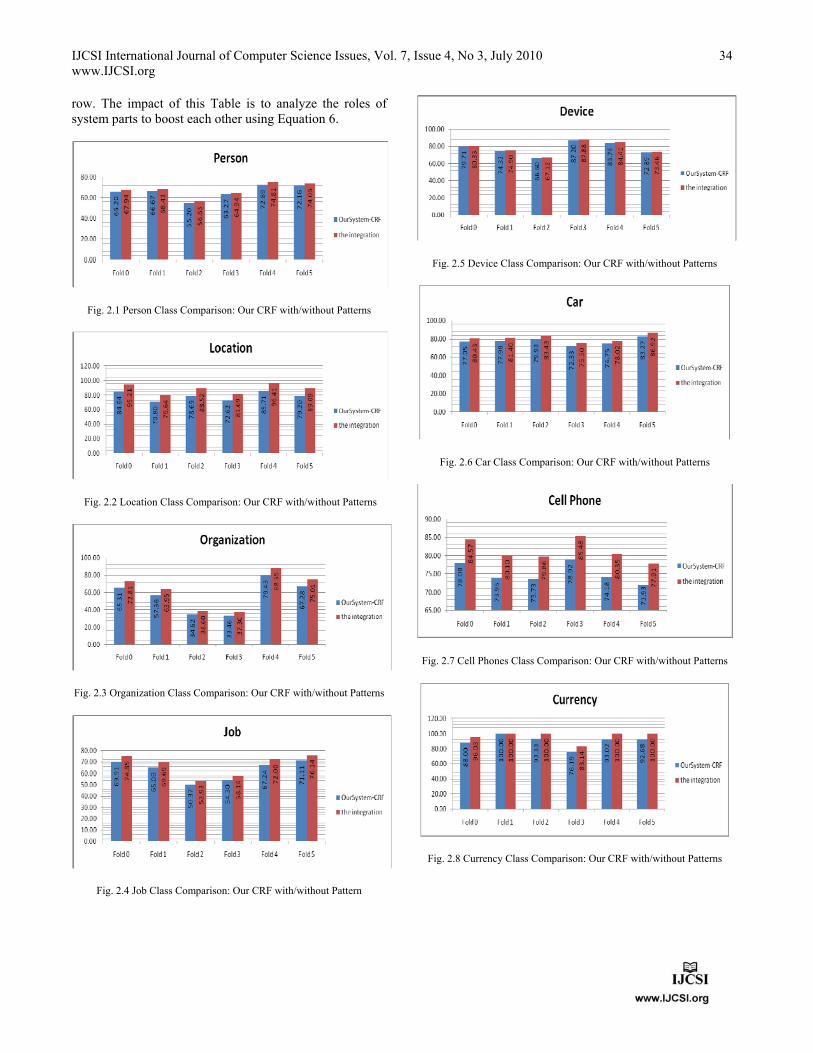
IJCSI International Journal of Computer Science Issues, Vol. 7, Issue 4, No 3, July 2010 www.IJCSI.org
34
row. The impact of this Table is to analyze the roles of system parts to boost each other using Equation 6.
Fig. 2.1 Person Class Comparison: Our CRF with/without Patterns
Fig. 2.2 Location Class Comparison: Our CRF with/without Patterns
Fig. 2.3 Organization Class Comparison: Our CRF with/without Patterns
Fig. 2.4 Job Class Comparison: Our CRF with/without Pattern
Fig. 2.5 Device Class Comparison: Our CRF with/without Patterns
Fig. 2.6 Car Class Comparison: Our CRF with/without Patterns
Fig. 2.7 Cell Phones Class Comparison: Our CRF with/without Patterns
Fig. 2.8 Currency Class Comparison: Our CRF with/without Patterns
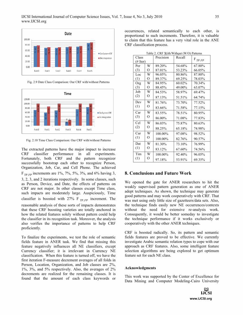
IJCSI International Journal of Computer Science Issues, Vol. 7, Issue 4, No 3, July 2010 www.IJCSI.org
35
Fig. 2.9 Date Class Comparison: Our CRF with/without Patterns
Fig. 2.10 Time Class Comparison: Our CRF with/without Patterns
The extracted patterns have the major impact to increase CRF classifier performance in all experiments. Fortunately, both CRF and the pattern recognizer successfully bootstrap each other to recognize Person, Organization, Job, Car, and Cell Phone. The achieved
F FPTP. increments are 1%, 7%, 5%, 3%, and 6% having 3,
3, 2, 3, and 2 iterations respectively. In some classes, such as Person, Device, and Date, the effects of patterns on CRF are not major. In other classes except Time class, such impacts are moderately large. Auspiciously, Time
classifier is boosted with 27% F FPTP , increment. The
reasonable analysis of these sorts of impacts demonstrates that these CRF boosting varieties are totally anchored in how the related features solely without pattern could help the classifier in its recognition task. Moreover, the analysis also verifies the importance of patterns to help CRF proficiently. To finalize the experiments, we test the role of semantic fields feature in ANER task. We find that missing this feature negatively influences all NE classifiers, except Currency classifier; it is irrelevant in Currency NE classification. When this feature is turned off, we have the first iteration F-measure decrement averages of all folds in Person, Location, Organization, and Job classes are 2%, 1%, 3%, and 5% respectively. Also, the averages of 2% decrements are realized for the remaining classes. It is found that the amount of each class keywords or
occurrences, related semantically to each other, is proportional to such increments. Therefore, it is valuable to claim that this feature has a very vital role in the ANE CRF classification process.
Table 2. CRF With/Without (W/O) Patterns Class (# Iter)
Precision Recall F FPTP.
Per (3)
W O
89.20% 54.68% 67.80% 87.01% 53.23% 66.05%
Loc (1)
W O
96.05% 80.86% 87.80% 89.37% 69.25% 78.03%
Org (3)
W O
84.95% 60.02% 70.34% 88.45% 49.00% 63.07%
Job (2)
W O
84.53% 58.97% 69.47%
87.13% 51.51% 64.74% Dev (1)
W O
81.76% 73.70% 77.52%
83.66% 71.58% 77.15% Car (3)
W O
83.55% 78.51% 80.95%
86.00% 71.08% 77.83% Cel (2)
W O
86.03% 75.87% 80.63%
88.25% 65.18% 74.98% Cur (1)
W O
100.00% 97.08% 98.52%
100.00% 82.76% 90.57% Dat (1)
W O
81.30% 73.10% 76.99%
83.12% 67.60% 74.56% Tim (1)
W O
100.00% 92.40% 96.05%
97.18% 53.91% 69.35%
8. Conclusions and Future Work
We opened the gate for ANER researchers to hit the weakly supervised pattern generation as one of ANER adept techniques. As shown, the technique may generate good patterns and may work cooperatively with CRF. That was met using only little size of gazetteers/data sets. Also, the technique finds easily new NE occurrences/contexts without the need for extensive re-analysis work. Consequently, it would be better someday to investigate the technique performance if it works exclusively or cooperatively with the other ANER techniques. CRF is boosted radically. So, its pattern and semantic fields features are proved to be effective. We currently investigate Arabic semantic relation types to cope with our approach as CRF features. Also, some intelligent feature selection algorithms are being explored to get optimum feature set for each NE class.
Acknowledgments
This work was supported by the Center of Excellence for Data Mining and Computer Modeling-Cairo University
IJCSI International Journal of Computer Science Issues, Vol. 7, Issue 4, No 3, July 2010 www.IJCSI.org
36
through Information Technology Industry Development Agency funds. All authors thank profoundly Engineer Amr Magdy Gomaa, a NLP researcher, for his endless contributions through the research experimental phase.
Samir AbdelRahman is an Assistant Professor at Computer Science Department, Faculty of Computers and Information, Cairo University. His M.Sc. and Ph.D. have been received from Cairo University in Computer Science Specialty. He is interested in Machine Learning, Named Entity Extraction, Text Mining, and NLP parsers. His research papers have been published mainly in Computational Linguistics/ Informatica journals and Coling conferences. His Arabic Opinion Mining work is supported and funded by the Center of Excellence for Data Mining and Computer Modeling-Cairo University.
Mohamed Elarnaoty is a Teaching Assistant at Computer Science Department, Faculty of Computers and Information, Cairo University. He is interested in Mathematics, Machine Learning, Named Entity Extraction, Opinion Mining, and NLP parsers.
Marwa Magdy is a Teaching Assistant at Computer Science Department, Faculty of Computers and Information, Cairo University. Her research interests are in Arabic NLP: Intelligent Language Tutoring System, Spelling Checkers, Named Entity Extraction, and Opinion Mining.
Aly Fahmy is a Professor at Computer Science Department, Faculty of Computers and Information, Cairo University. He is the Principle Investigator of the Center of Excellence for Data Mining and Computer Modeling-Cairo University. His research concerns mainly in Computational Linguistics, Text Mining, Data Mining, and Software Engineering. References [1] S.Abuleil, “Extracting Names From Arabic Text For
Question-Answering Systems”, 7th International Conference of Computer-Assisted Information Retrieval Applications, University of Avignon, RIAO 2004, France.
[2] M.Attia and M.Rashwan, “A Large Scale Arabic POS Tagger Based on a Compact Arabic POS Tag Set and Application on the Statistical Inference of Syntactic Diacritics of Arabic Text Words”, NEMLAR, 2004.
[3] M.Attia, M.Rashwan, A.Ragheb, M.A.H Al-Basoumy, and S.Abdou. “A Compact Arabic Lexical Semantics Language Resource Based on the Theory of Semantic Fields”, Proceedings of the 6th international conference on Advances in Natural Language Processing, 2008.
[4] Y.Benajiba , M.Diab, and P.Rosso, “Arabic Named Entity Recognition using Optimized Feature Sets”, EMNLP 2008: 284-293.
[5] Y.Benajiba, and P.Rosso, “Arabic Named Entity Recognition using Conditional Random Field, 6th Int. Conf. on Language Resources and Evaluation”, LREC 2008.
[6] Y.Benajiba and P.Rosso, “ANERsys 2.0: Conquering the NER Task for the Arabic Language by Combining the Maximum Entropy with POS-tag Information”, Workshop on Natural Language-Independent Engineering, 3rd Indian Int. Conf. on Artificial Intelligence, Pune, India, 2007.
[7] S.Brin, “Extracting Patterns and Relations form the World Wide Web”, WebDB Workshop at EDBT, 1998.
[8] Z.Chen and H.Ji, “Can One Language Bootstrap the Other: A Case Study on Event Extraction”, Proc. HLT-NAACL,
Workshop on Semi-supervised Learning for Natural Language Processing. Boulder, 2009.
[9] A.Elsebai, F.Meziane, and F.Z.BelKredim, “A Rule Based Persons Names Arabic Extraction System”, in Communications of the IBIMA Volume 11, ISSN: 1943-7765, 2009.
[10] G.Forman and M.Scholz, “Apples-to-Apples in Cross-Validation Studies: Pitfalls in Classifier Performance Measurement” , HP technical Reports, HPL-2009-359, 2009.
[11] I.Guyon and A.Elisseeff, “An Introduction to Variable and Feature Selection”, Journal of Machine Learning Research 3 (2003) 1157-1182, 2003.
[12] A.Hassan, H.Fahmy, and H.Hassan, “Improving Named Entity Translation by Exploiting Comparable and Parallel Corpora”, RANLP, AMML Workshop, 2007.
[13] H.Hassan and J.Sorensen, “An Integrated Approach for Arabic-English Named Entity Translation”, Proceedings of the ACL Workshop on Computational Approaches to Semitic Languages, 2005.
[14] H.Ji and R.Grishman, “Data Selection in Semi-supervised Learning for Name Tagging”, In Proceedings of COLING/ACL 06 Workshop on Information Extraction Beyond Document, Sydney, Australia, 2006.
[15] Z.Kozareva, “Bootstrapping Named Entity Recognition with Automatically Generated Gazetteer Lists”, In Proceedings of EACL 2006, Trento, Italy, April 2006.
[16] T.Kudo and Y.Matsumoto, “Use of Support Vector Learning for Chunk Identification”, CoNLL-2000.
[17] J.Lafferty, A.McCallum, and F.Pereira, “Conditional random fields: Probabilistic models for segmenting and labeling sequence data”, In Proc. of ICML, pp.282-289, 2001.
[18] J.Maloney and M.Niv, “TAGARAB: A Fast, Accurate Arabic Name Recognizer Using High Precision Morphological Analysis”, In Proceedings of the Workshop on Computational Approaches to Semitic Languages, Canada, 1998.
[19] D.Samy, A.Moreno, and J.M.Guirao, “A Proposal For An Arabic Named Entity Tagger Leveraging a Parallel Corpus (Spanish-Arabic)”, In Proceedings of Recent Advances in Natural Language Processing RANLP, Borovets, Bulgaria, pp. 459-465. 2005.
[20] K.Shaalan and H.Raza, “NERA: Named Entity Recognition for Arabic”, The Journal of the American Society for Information Science and Technology (JASIST), John Wiley & Sons, Inc., NJ, USA, 60(8): 1652–1663, 2009.
[21] D.Wu, W.S.Lee, N.Ye, and H.L.Chieu, “Domain Adaptive Bootstrapping for Named Entity Recognition”, Proceedings of the 2009 Conference on Empirical Methods in Natural Language Processing, pages 1523–1532, Singapore, ACL and AFNLP, 2009.
[22] J.Zhu, Z.Nie, X.Liu, B.Zhang, and J.Wen, “StatSnowball: A Statistical Approach to Extracting Entity Relationships”, WWW 2009 Madrid, 2009.

IJCSI International Journal of Computer Science Issues, Vol. 7, Issue 4, No 3, July 2010 ISSN (Online): 1694-0784 ISSN (Print): 1694-0814
37
A New Approach for Optimal Clustering of Distributed Program's Call Flow Graph
Yousef Abofathy1, Bager Zarei2
1 Department of Computer Engineering, Islamic Azad University, Shabestar Branch Tabriz, East-Azarbaijan, Iran
2 Department of Computer Engineering, Islamic Azad University, Shabestar Branch Tabriz, East-Azarbaijan, Iran
Abstract
Optimal clustering of call flow graph for reaching maximum concurrency in execution of distributable components is one of the NP-Complete problems. Both learning automatas (LAs) and genetic algorithms (GAs) are search tools which are used for solving many NP-Complete problems. In this paper a hybrid algorithm is proposed to optimal clustering of call flow graph and appropriate distributing of programs in network level. The algorithm uses both GAs and LAs simultaneously to search in state space. It has been shown that the speed of reaching to solution increases remarkably using LA and GA simultaneously in search process, and it also prevents algorithm from being trapped in local minimums. Experimental results show the superiority of proposed algorithm over others. Keywords: Call Flow Graph, Clustering, Learning Automata, Genetic Algorithm, Concurrency, Distributed Code.
1. Introduction
Optimization of distributed code with goal of achieving maximum concurrency in execution of distributable components in network level is considered as a new aspect in optimization discussions. Concurrency in execution of distributed code is obtained from remote asynchronous calls. The problem is specifying appropriate calls, with considering amount of yielding concurrency from remote asynchronous calls. In this way, dependency graph between objects are clustered with the base of amount of calls between objects, and each cluster is considered as a component in distributed architecture. Since clustering is a NP-Complete problem, in this paper a hybrid non-deterministic algorithm is proposed for optimal clustering of call flow graph. The proposed algorithm uses both GAs and LAs simultaneously to search in state space. With the combination of the GA and LA, and incorporation of concepts of gene, chromosome, action and depth, background of the evolution of problem's solution was extracted effectively and is used in the search process.
Resisting against the superficial changes of solutions is the most important characteristic of proposed algorithm. In other words, there is a flexible balance between the effectiveness of GA and stability of LA in proposed algorithm. Self-recovery, reproduction, penalty and reward are characteristics of proposed algorithm.
2. Genetic algorithms
GAs act on the basis of evolution in nature, and search for the final solution among a population of potential solutions. In every generation the fittest individuals of that generation are selected and after recombination, produce a new set of children. In this process the fittest individuals will survive more probably in next generations. At the beginning of algorithm a number of individuals (initial population) are created randomly and the fitness function is evaluated for all of them. If termination condition does not satisfied, parents are selected based on their fitness and are recombined. Then produced children mutate with a fixed probability and their fitness values are calculated. Next new population (generation) is generated by replacing of children with parents, and this process is repeated until the termination condition is satisfied.
3. Learning automata
Learning in LAs is choosing an optimal action from a set of automata's allowable actions. This action is applied on a random environment and the environment gives a random answer to this action from a set of allowable answers. The environment's answer depends statistically on the automata's action. The environment term includes a collection of all outside conditions and their effects on the automata's operation. The interaction between environment and LA is shown in figure 1.
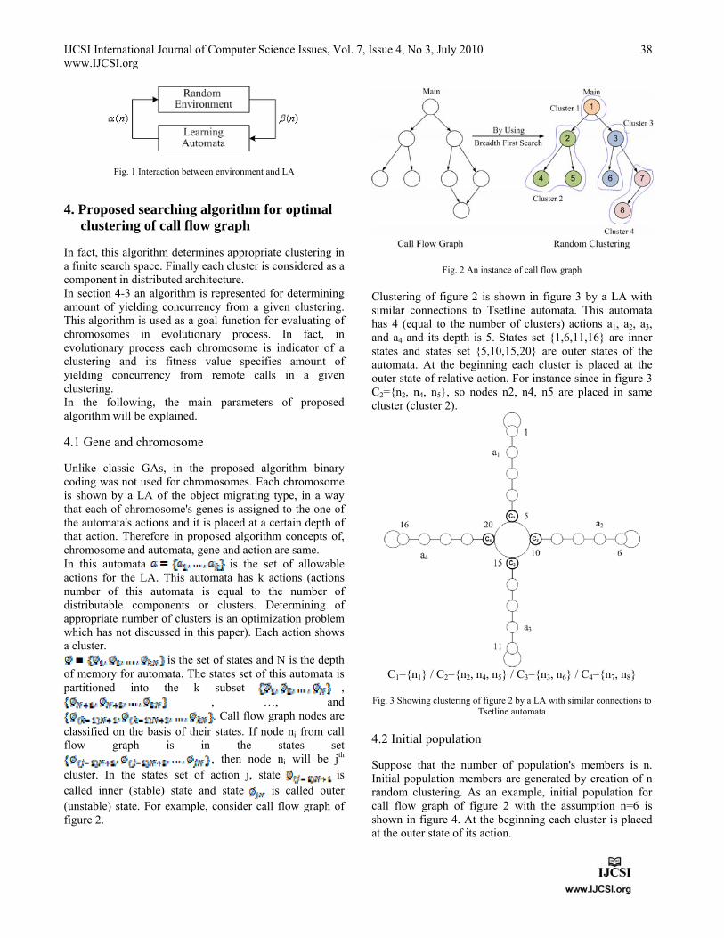
IJCSI International Journal of Computer Science Issues, Vol. 7, Issue 4, No 3, July 2010 www.IJCSI.org
38
Fig. 1 Interaction between environment and LA
4. Proposed searching algorithm for optimal clustering of call flow graph
In fact, this algorithm determines appropriate clustering in a finite search space. Finally each cluster is considered as a component in distributed architecture. In section 4-3 an algorithm is represented for determining amount of yielding concurrency from a given clustering. This algorithm is used as a goal function for evaluating of chromosomes in evolutionary process. In fact, in evolutionary process each chromosome is indicator of a clustering and its fitness value specifies amount of yielding concurrency from remote calls in a given clustering. In the following, the main parameters of proposed algorithm will be explained.
4.1 Gene and chromosome
Unlike classic GAs, in the proposed algorithm binary coding was not used for chromosomes. Each chromosome is shown by a LA of the object migrating type, in a way that each of chromosome's genes is assigned to the one of the automata's actions and it is placed at a certain depth of that action. Therefore in proposed algorithm concepts of, chromosome and automata, gene and action are same. In this automata is the set of allowable actions for the LA. This automata has k actions (actions number of this automata is equal to the number of distributable components or clusters. Determining of appropriate number of clusters is an optimization problem which has not discussed in this paper). Each action shows a cluster.
is the set of states and N is the depth of memory for automata. The states set of this automata is partitioned into the k subset ,
, …, and . Call flow graph nodes are
classified on the basis of their states. If node ni from call flow graph is in the states set
, then node ni will be jth cluster. In the states set of action j, state is called inner (stable) state and state is called outer (unstable) state. For example, consider call flow graph of figure 2.
Fig. 2 An instance of call flow graph
Clustering of figure 2 is shown in figure 3 by a LA with similar connections to Tsetline automata. This automata has 4 (equal to the number of clusters) actions a1, a2, a3, and a4 and its depth is 5. States set {1,6,11,16} are inner states and states set {5,10,15,20} are outer states of the automata. At the beginning each cluster is placed at the outer state of relative action. For instance since in figure 3 C2={n2, n4, n5}, so nodes n2, n4, n5 are placed in same cluster (cluster 2).
C1={n1} / C2={n2, n4, n5} / C3={n3, n6} / C4={n7, n8}
Fig. 3 Showing clustering of figure 2 by a LA with similar connections to Tsetline automata
4.2 Initial population
Suppose that the number of population's members is n. Initial population members are generated by creation of n random clustering. As an example, initial population for call flow graph of figure 2 with the assumption n=6 is shown in figure 4. At the beginning each cluster is placed at the outer state of its action.
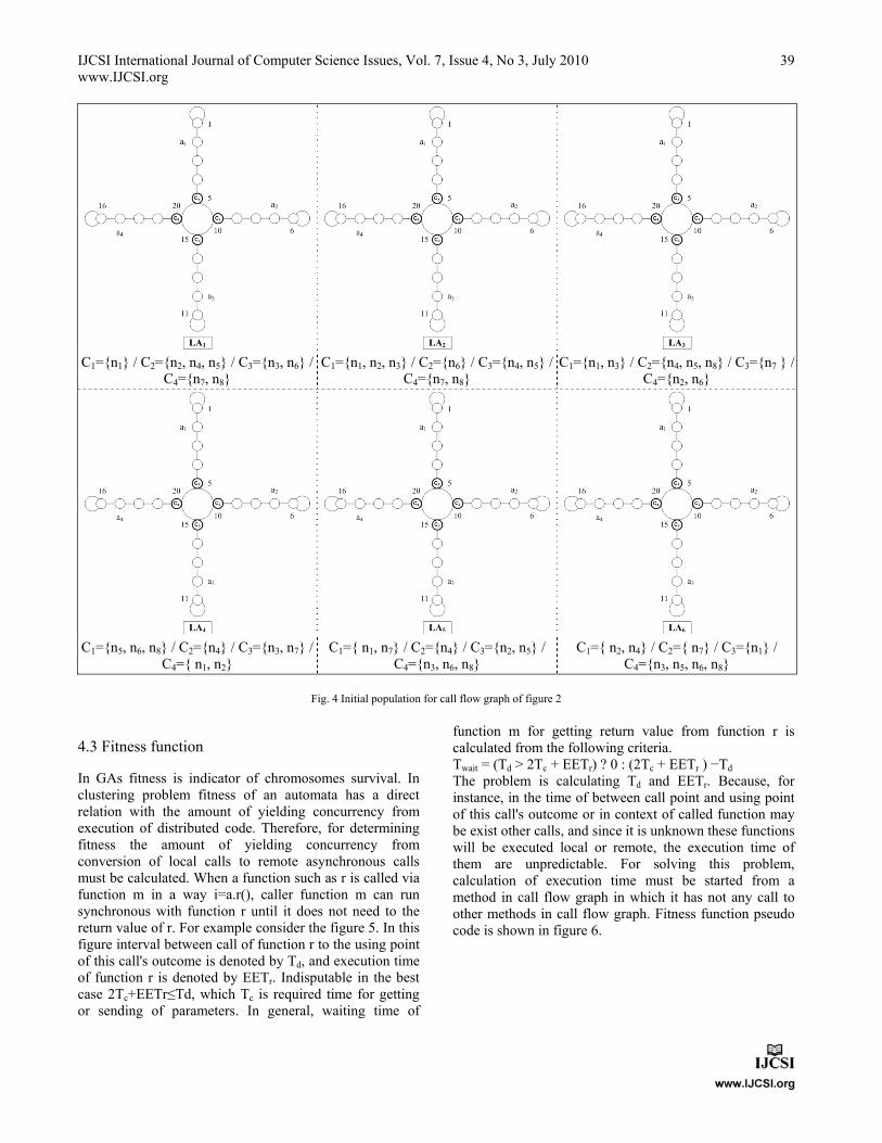
IJCSI International Journal of Computer Science Issues, Vol. 7, Issue 4, No 3, July 2010 www.IJCSI.org
39
C1={n1, n3} / C2={n4, n5, n8} / C3={n7 } /
C4={n2, n6}C1={n1, n2, n3} / C2={n6} / C3={n4, n5} /
C4={n7, n8} C1={n1} / C2={n2, n4, n5} / C3={n3, n6} /
C4={n7, n8}
C1={ n2, n4} / C2={ n7} / C3={n1} /
C4={n3, n5, n6, n8}C1={ n1, n7} / C2={n4} / C3={n2, n5} /
C4={n3, n6, n8}C1={n5, n6, n8} / C2={n4} / C3={n3, n7} /
C4={ n1, n2}
Fig. 4 Initial population for call flow graph of figure 2
4.3 Fitness function
In GAs fitness is indicator of chromosomes survival. In clustering problem fitness of an automata has a direct relation with the amount of yielding concurrency from execution of distributed code. Therefore, for determining fitness the amount of yielding concurrency from conversion of local calls to remote asynchronous calls must be calculated. When a function such as r is called via function m in a way i=a.r(), caller function m can run synchronous with function r until it does not need to the return value of r. For example consider the figure 5. In this figure interval between call of function r to the using point of this call's outcome is denoted by Td, and execution time of function r is denoted by EETr. Indisputable in the best case 2Tc+EETr≤Td, which Tc is required time for getting or sending of parameters. In general, waiting time of
function m for getting return value from function r is calculated from the following criteria. Twait = (Td > 2Tc + EETr) ? 0 : (2Tc + EETr ) −Td The problem is calculating Td and EETr. Because, for instance, in the time of between call point and using point of this call's outcome or in context of called function may be exist other calls, and since it is unknown these functions will be executed local or remote, the execution time of them are unpredictable. For solving this problem, calculation of execution time must be started from a method in call flow graph in which it has not any call to other methods in call flow graph. Fitness function pseudo code is shown in figure 6.

IJCSI International Journal of Computer Science Issues, Vol. 7, Issue 4, No 3, July 2010 www.IJCSI.org
40
Fig. 5 Calculation of exection time in remote calls
Function FitnessEvaluation(CallFlowGraph, Clusters):Speedup Begin Call TopologicalSort(CallFlowGraph); for each method m in call flow graph if NoCallsm = 0 then EETm = 0; for each not call statement, i, within m EETm = EETm + ExecutionTime(i); for each local call statement, c, within m EETm = EETm + EETc; for each remote asynchronous call statement, r, within m EETm = EETm + Max(Td, 2Tc + EETr); for each parent, p, of m within the call flow graph NoCallsp = NoCallsp – 1; End if End for End function
Fig. 6 Fitness function pseudo code
4.4 Operators
Since in proposed algorithm, every chromosome is shown in the form of LA, crossover and mutation operators are not similar to genetic traditional operators. a) Selection operator: In order to choose LAs (chromosomes) for recombination or mutation operators, one of these methods can be used: Ranking Selection, Roulette Wheel Selection, and Tournament Selection. b) Crossover operator: To do this operator a new method is proposed for working with sets namely NewCrossover. In this method two nodes ni and nj are selected randomly from call flow graph and their relative actions is swapped in two parents. With doing this operator two new automatas are created which are called children of two parents. For example, suppose that LA2 and LA5 automatas are selected randomly as parents from the previously formed population. By random selection of two nodes n3 and n7
from call flow graph and swapping their relative actions in
two parents, two new automats are created. This is shown in figure 7. c) Mutation operator: To do this operator a node ni is selected randomly from call flow graph and its action is swapped randomly. State of random node n5 before and after mutation is shown in figure 8. d) Penalty and reward operator: Since in proposed algorithm, every chromosome is shown in the form of LA, in each automata after examining fitness of a cluster (action) which is selected randomly, that cluster will be rewarded or penalized. State of a cluster in the relative action states set will be changed as the result of rewarding or penalizing it. If a cluster is placed at the outer state of an action, penalizing it leads to action of one of its nodes is changed and so a new clustering will created. The rate of this operator should be low, because this operator is a random search operator, and reduces the effectiveness of algorithm if it is applied with high rate. Reward and penalty operator vary according to the LA types. For example, in an automata with similar connections to Tsetline automata if cluster C3 is in the states set {11, 12, 13, 14, 15}, and its execution time without considering remote calls is less than threshold, this cluster is rewarded and it moves to the inner states of its action. If cluster C3 is in the innermost state (state number 11) and rewarded, it will remain in that state. The movement of such cluster is shown in figure 9. If execution time of a cluster without considering remote calls is greater than threshold, this cluster is not appropriate and it is penalized. The movement of such cluster for two different cases is as follows: a) The cluster is at a state other than outer state: Panelizing this cluster reduces its importance and it moves to the outer states. The movement of such cluster is shown in figure 10. b) The cluster is in outer state: In this case, we find a cluster of automata in which, if one of the cluster nodes is moved to the founded cluster, maximum increase in fitness outcome. In this case, if the founded cluster is not in outer state, first it is moved to outer state of its action and then node is moved to it. The movement of such cluster is shown in figure 11. Important subject is determining of threshold value. For this consider concurrent execution time in following three different cases: Best Case (100% Concurrency):
Average Case (50% Concurrency):
Worst Case (0% Concurrency):
In above criteria, Tc is concurrent execution time, Ts is sequent execution time, and NoClusters is number of clusters. In this paper we considered threshold value be concurrent execution time in average case.
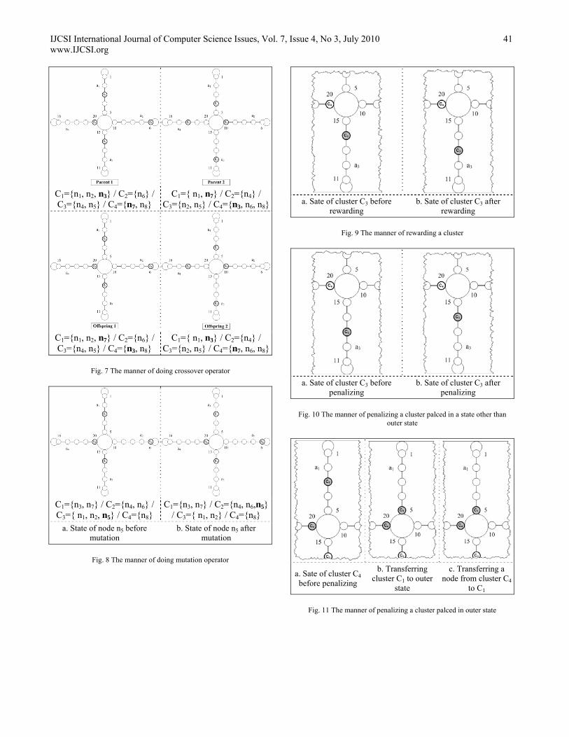
IJCSI International Journal of Computer Science Issues, Vol. 7, Issue 4, No 3, July 2010 www.IJCSI.org
41
C1={ n1, n7} / C2={n4} /
C3={n2, n5} / C4={n3, n6, n8}C1={n1, n2, n3} / C2={n6} / C3={n4, n5} / C4={n7, n8}
C1={ n1, n3} / C2={n4} /
C3={n2, n5} / C4={n7, n6, n8}C1={n1, n2, n7} / C2={n6} / C3={n4, n5} / C4={n3, n8}
Fig. 7 The manner of doing crossover operator
C1={n3, n7} / C2={n4, n6,n5}
/ C3={ n1, n2} / C4={n8}C1={n3, n7} / C2={n4, n6} / C3={ n1, n2, n5} / C4={n8}
b. State of node n5 after mutation
a. State of node n5 before mutation
Fig. 8 The manner of doing mutation operator
b. Sate of cluster C3 after rewarding
a. Sate of cluster C3 before rewarding
Fig. 9 The manner of rewarding a cluster
b. Sate of cluster C3 after penalizing
a. Sate of cluster C3 before penalizing
Fig. 10 The manner of penalizing a cluster palced in a state other than outer state
c. Transferring a
node from cluster C4 to C1
b. Transferring cluster C1 to outer
state
a. Sate of cluster C4 before penalizing
Fig. 11 The manner of penalizing a cluster palced in outer state

IJCSI International Journal of Computer Science Issues, Vol. 7, Issue 4, No 3, July 2010 www.IJCSI.org
42
Proposed algorithm pseudo code is shown in figure 12.
Function CFG_Clustering(CallFlowGraph):Clusters Begin n = Size of Population; Create the initial population LA1 … LAn; FitnessEvaluation(CallFlowGraph, LAi); //for all LAs while(Termination Condition not Satisfied) do NewLA1 = NewLA2 = LA with minimum Value of Execution Time; //move best two individuals to the new population
for i = 2 to n do //Create new population Select LA1; Select LA2 ; if (Random ≤ CrossoverRate) then Crossover(LA1, LA2); if (Random ≤ MutationRate) then Mutation(LA1); Mutation(LA2); NewLAi+1 = LA1; NewLAi+2 = LA2 ; i=i+2; end for for i = 1 to n do //Replace old population with new population
LAi = NewLAi; Cj = Random * NoClusters; if (ExecutionTime(LAi.Cj) < Threshold) then Reward(LAi , Cj); else Penalize(LAi , Cj); end for FitnessEvaluation(CallFlowGraph, LAi); //for all LAs end while End function
Fig. 12 Proposed algorithm pseudo code
5. Proposed method evaluation
In order to evaluating proposed algorithm, distributed code of implementation of TSP was used. This distributed code solves TSP by using dynamic methods and finding optimal spanning tree. Table and diagram 1 shows execution time of TSP program for three cases sequential, distributed by reference [2] algorithm clustering, and distributed by proposed algorithm clustering for graphs with different node and edges number. As you observed average execution time of TSP program by proposed algorithm clustering is less than average execution time of sequential and distributed by reference [2] algorithm clustering. This shows that proposed algorithm is efficient than other algorithms, and it can be used for clustering of call flow graph of large application programs.
Table 1: Execution time of TSP program for three cases sequential, distributed by reference [2] algorithm clustering, and distributed by
proposed algorithm clustering for graphs with different node and edges number
Num
ber
of G
raph
N
odes
Num
ber
of G
raph
E
dge
s
Seq
uen
tial
E
xecu
tion
Tim
e
Dis
trib
uted
E
xecu
tion
Tim
e w
ith
Ref
eren
ce [
2]
Alg
orit
hm
C
lust
erin
g D
istr
ibut
ed
Exe
cuti
on T
ime
wit
h P
rop
osed
A
lgor
ith
m
Clu
ster
ing
20 40 0.573 7.357 4.347
40 81 1.383 7.810 5.057
60 122 3.246 8.163 6.163
80 163 11.214 11.109 8.713
100 204 19.773 14.741 10.677
120 245 43.517 30.722 22.222
140 286 85.362 60.871 46.546
160 327 145.721 105.227 73.379
180 368 234.871 168.280 112.511
200 409 360.143 261.412 196.615
220 450 576.655 440.343 316.741
240 491 997.653 774.142 542.524
Average Execution Time (Second) 206.6759 157.5148 112.125
Diagram 1: Execution time of TSP program for three cases sequential, distributed by reference [2] algorithm clustering, and distributed by
proposed algorithm clustering for graphs with different node and edges number
6. Conclusion
Problem of finding optimal distribution for reaching maximum concurrency in distributed programs is a NP-Complete problem. So, Deterministic methods are not appropriate for this problem. In this paper an evolutionary

IJCSI International Journal of Computer Science Issues, Vol. 7, Issue 4, No 3, July 2010 www.IJCSI.org
43
non-deterministic method is proposed for this problem. Proposed method uses both GAs and LAs simultaneously to search in state space. Evaluation results and amount of yielding concurrency from using proposed algorithm, indicator of proposed method efficiency over others. References [1] S. Parsa, and O. Bushehrian, "Performance-Driven Object-
Oriented Program Remodularization", ISSN: 1751-8806, INSPEC Accession Number: 10118318, Digital Object Identifier: 10.1049/iet-sen: 20070065, Aug, 2008.
[2] S. Parsa, and V. Khalilpoor, "Automatic Distribution of Sequential Code Using JavaSymphony Middleware", 32th International Conference On Current Trends in Theory and Practice of Computer Science, 2006.
[3] Roxana Diaconescu, Lei Wang, Zachary Mouri, and Matt Chu, "A Compiler and Runtime Infrastructure for Automatic Program Distribution", 19th International Parallel and Distributed Processing Symposium (IPDPS 2005), IEEE, 2005.
[4] S. Parsa, O. Bushehrian, "The Design and Implementation of a Tool for Automatic Software Modularization", Journal of Supercomputing, Volume 32, Issue 1, April 2005.
[5] Mohammad M. Fuad, and Michael J. Oudshoorn, "AdJava-Automatic Distribution of Java Applications", 25th Australasian Computer Science Conference (ACSC2002), Monash University, Melbourne, 2002.
[6] S. Mitchell Brian, "A Heuristic Search Approach to Solving the Software Clustering Problem", Thesis, Drexel University, March 2002.
[7] Thomas Fahringer, and Alexandru Jugravu, "JavaSymphony: New Directives to Control and Synchronize Locality, Parallelism, and Load Balancing for Cluster and GRID-Computing", Proceedings of Joint ACM Java Grande ISCOPE 2002 Conference, Seattle, Washington, Nov 2002.
[8] Michiaki Tatsubori, Toshiyuki Sasaki, Shigeru Chiba1, and Kozo Itano, "A Bytecode Translator for Distributed Execution of Legacy Java Software", LNCS 2072, pp. 236-255, 2001.
[9] Markus Dahm, "Doorastha—A Step Towards Distribution Transparency", JIT, 2000.
[10] Michael Philippsen, and Bernhard Haumacher, "Locality Optimization in JavaParty by Means of Static Type Analysis", Concurrency: Practice & Experience, pp. 613-628, July 2000.
[11] Andre Spiegel, "Pangaea: An Automatic Distribution Front-End for Java", 4th IEEE Workshop on High-Level Parallel Programming Models and Supportive Environments (HIPS '99), San Juan, Puerto Rico, April 1999.
[12] Saeed Parsa, and Omid Bushehrian, "Genetic Clustering with Constraints", Journal of Research and Practice in Information Technology, 2007.
[13] Leng Mingwei, Tang Haitao, and Chen Xiaoyun, "An Efficient K-means Clustering Algorithm Based on Influence Factors", Eighth ACIS Int. Conference on Software Engineering, Artificial Intelligence, Networking, and Parallel/Distributed Computing, pp. 815-820, July 2007.
[14] Tapas Kanungo, David M. Mount, Nathan S. Netanyahu, Christine D. Piatko, Ruth Silverman, and Angela Y. Wu,
"An Efficient K-Means Clustering Algorithm: Analysis and Implementation", IEEE Transaction on Pattern Analysis and Machine Intelligence, Vol. 24, No. 7, July 2002.
[15] Tapas Kanungo, David M. Mount, Nathan S. Netanyahu, Christine D. Piatko, Ruth Silverman, and Angela Y. Wu, "The Analysis of a Simple K-Means Clustering Algorithm", Proc. of the Sixteenth Annual Symposium on Computational Geometry, pp. 162, June 2000.
[16] B. Hendrickson, and R. Leland, "A Multilevel Algorithm for Partitioning Graphs", Proceedings of the 1995 ACM/IEEE Conference on Supercomputing (CDROM), pp. 28, ACM Press, 1995.
[17] V. R. Vemuri, "Genetic Algorithms”, Computer Society meeting, Department of Applied Science, University of California, 1997.
[18] E. Cantu-Paz, "A Survey of Parallel Genetic Algorithms", IlliGAL Reprot, No. 97003, May 1997.
[19] D. E. Goldberg, "Genetic Algorithms in Search, Optimization and Machine Learning", Reading, MA, Addition-Wesley, 1989.
[20] F. Busetti, "Genetic Algorithm Overview". [21] K. A. Dejong , and W. M. Spears, "Using Genetic
Algorithms to Solve NP-Complete Problems", Proceedings of the Third International Conference on Genetic Algorithms, 1989.
[22] K. S. Narendra, and M. A. L. Thathachar, "Learning Automata: An Introduction", Prentice-hall, Englewood cliffs, 1989.
[23] M. R. Meybodi, and H. Beigy, "Solving Graph Isomorphism Problem by Learning Automata", Thesis, Computer Engineering Faculty, Amirkabir Technology University, Tehran, Iran, 2000.
[24] H. Beigy, and M. R. Meybodi, "Optimization of Topology of Neural Networks Using Learning Automata", Proceedings of 3th Annual International Computer Society of Iran Computer Conference (CSICC-98), Tehran, Iran, pp. 417-428, 1999.
[25] B. J. Oommen, R. S. Valiveti, and J. R. Zgierski, "An Adaptive Learning Solution to the Keyboard Optimization Problem", IEEE Transaction On Systems. Man. And Cybernetics, Vol. 21, No. 6, pp. 1608-1618, 1991.
[26] B. J. Oommen, and D. C. Y. Ma, "Deterministic Learning Automata Solution to the Keyboard Optimization Problem", IEEE Transaction on Computers, Vol. 37, No. 1, pp. 2-3, 1988.
[27] A. A. Hashim, S. Amir, and P. Mars, "Application of Learning Automata to Data Compression", in Adaptive and Learning Systems, K. S. Narendra, Editor, New York, Plenum Press, pp. 229-234, 1986.
[28] M. R. Meybodi, and S. Lakshmivarhan, "A Learning Approach to Priority Assignment in a Two Class M/M/1 Queuing System with Unknown Parameters", Proceedings of Third Yale Workshop on Applications of Adaptive System Theory, Yale University, pp. 106-109, 1983.
[29] Bager Zarei, M. R. Meybodi, and Mortaza Abbaszadeh, "A Hybrid Method for Solving Traveling Salesman Problem", Proceedings of the 6th IEEE/ACIS International Conference on Computer and Information Science (ICIS 2007), IEEE Computer Society, Melbourne, Australia, pp. 394-399, 11-13 July 2007.

IJCSI International Journal of Computer Science Issues, Vol. 7, Issue 4, No 3, July 2010 ISSN (Online): 1694-0784 ISSN (Print): 1694-0814 44
An Effective Solution to Reduce Count-to-Infinity Problem in Ethernet
1Ganesh.D, 2 Venkata Rama Prasad Vaddella
1Assistant Professor, Department of Information Technology
Sree Vidyanikethan Engineering College, Tirupati-517 102, India
2 Professor and Head Department of Information Technology
Sree Vidyanikethan Engineering College, Tirupati-517 102, India
Abstract
Ethernet is currently the most popular networking technology because of its high performance, low cost and ubiquity nature. Ethernets rely on the dynamic computation of a cycle-free active forwarding topology. For that it uses rapid spanning tree protocol. Unfortunately, it exhibits count-to-infinity problem that may lead to forwarding loops under certain network failures. These consequences are considered serious since network can become highly congested and even packet forwarding can fail. In this work, a simple and effective solution to reduce count-to-infinity problem, called RSTP with epochs is proposed. This eliminates the count-to-infinity induced forwarding loop and improves the convergence time.
Keywords: count-to-infinity, Ethernet, spanning tree protocols
1. Introduction
Ethernet is the mo st popular n etworking t echnology in a wide range of environments due to its high performance-to-cost rati o and u biquity. In existing et hernet sta ndards, packet flooding is used t o de liver a packet t o a ne w unknown destination address whose topological location in the ne twork is unknown. A n et hernet sw itch observes the flooding of packet to l earn the topological location of an address. A switch ide ntifies the por t a t w hich the packet from source S arrives. Then it uses this port for the packets whose destination a ddress is so urce S . Thus, a n e thernet network dynamically discovers the topological locations of interface a ddresses a nd dynamically builds pac ket forwarding t ables ac cordingly. This me chanism i s c alled address lea rning. Exi sting e thernet st andards use a “Spanning Tree Protocol” w hich com putes a cy cle-free active fo rwarding t opology to s upport t he flooding of packets for new destination and address learning. In case of link failure, c ycles in t he physical to pology p rovides a redundant pat h. It is ne cessary that t he a ctive forw arding topology to b e cycle free be cause ethernet pac kets ma y cause congestion due to the lack of time-to-live field. When a li nk or switch fa ilure occurs, it disturbs t he active forwarding topology, the network leads to a packet loss. The active forwarding topology is recomputed to stop the packet loss.
The de pendability of ethernet rel ies o n the ability of th e spanning t ree prot ocol to qu ickly recomputed cycle-free topology upon a partial network failure. In the present day, the rapid spanning tree protocol, RSTP [1] is the dominant spanning tree pr otocol. B ut unfortunately, RS TP m ay exhibit the count-to-infinity p roblem. Th e sp anning tree topology is c ontinuously reconfigured d uring t he count t o infinity and it form s the te mporary forw arding loop. T he ports i n t he network can oscillate between f orwarding and blocking da ta pa ckets. Thus, many da ta packets ma y be dropped. The forwarding loo p la sts un til the count t o infinity lasts. In the present work, count-to-infinity problem in RSTP is examined and an effective solution called RSTP with e pochs is presented. We dem onstrate the exact conditions under which the count to infinity problem occurs in RS TP and st udy the problem i n de tail with an e xample and identify the e ffects. This so lution improves the convergence time of t he s panning tree computation u pon failure.
In this work we perform an in -depth analysis of the count-to-infinity pr oblem an d pro vide a n effec tive s olution. In section-II, a brief introduction of Spanning trees & BPDU’s is given. S ection-III disc usses in detail a bout c ount-to-Infinity pro blem. Section-IV provides us t he solution for reducing c ount-to-infinity cal led RSTP with Epo chs. In Section-V, w e eva luate the protocol. S ection-VI de scribes the e ffects of count-to-Infinity on p ort sa turation an d a lso the results are evaluated. Conclusions of this work are given in section-VII.
2. Rapid Spanning Tree Protocol (RSTP)
The rapid spanning tree protocol (RSTP) was introduced in the IEEE 802.1W s tandard and later revised in the IEE E 802.1 D standards. RSTP was derived from Spanning Tree protocol (STP) and it i s des igned to o vercome STP’s long convergence time.
2.1. The Spanning Tree
RSTP computes a unique spanning tree over t he network of bridges a nd con necting l inks. Eac h bridge must have a unique ID. The spanning tree is rooted at the bridge with the lowest ID. There exists only one possible path between any
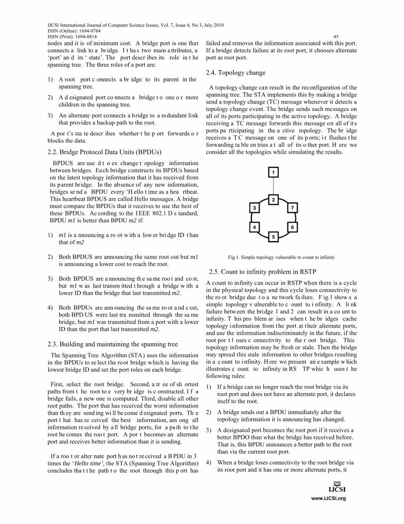
IJCSI International Journal of Computer Science Issues, Vol. 7, Issue 4, No 3, July 2010 ISSN (Online): 1694-0784 ISSN (Print): 1694-0814 45
nodes and it is of minimum cost. A bridge port is one that connects a link to a br idge. I t ha s two main a ttributes, a ‘port’ an d its ‘ state’. The port descr ibes its role in t he spanning tree. The three roles of a port are:
1) A root port c onnects a br idge to its parent in the spanning tree.
2) A d esignated port co nnects a bridge t o one o r more children in the spanning tree.
3) An alternate port connects a bridge to a redundant link that provides a backup path to the root.
A por t’s sta te descr ibes whether t he p ort forwards o r blocks the data.
2.2. Bridge Protocol Data Units (BPDUs) BPDUS are use d t o ex change t opology information between bridges. Each bridge constructs its BPDUs based on the latest topology information that it has received from its parent bridge. In the absence of any new information, bridges se nd a BPDU every ‘H ello t ime as a hea rtbeat. This heartbeat BPDUS are called Hello messages. A bridge must compare the BPDUs that it receives to use the best of these BPDUs. Ac cording to the I EEE 802.1 D s tandard, BPDU m1 is better than BPDU m2 if:
1) m1 is a nnouncing a ro ot w ith a low er bri dge ID t han that of m2
2) Both BPDUS are announcing the same root out but m1 is announcing a lower cost to reach the root.
3) Both BPDUS are a nnouncing th e sa me roo t and co st, but m1 w as last transm itted t hrough a bridge w ith a lower ID than the bridge that last transmitted m2.
4) Both BPDUs are ann ouncing the sa me ro ot a nd c ost, both BPD US were last tra nsmitted through the sa me bridge, but m1 was transmitted from a port with a lower ID than the port that last transmitted m2.
2.3. Building and maintaining the spanning tree The Spanning Tree Algorithm (STA) uses the information in the BPDUs to se lect the root bridge which is having the lowest bridge ID and set the port roles on each bridge.
First, select the root bridge. Second, a tr ee of sh ortest paths from t he root to e very br idge is c onstructed. I f a bridge fails, a new one is computed. Third, disable all other root paths. The port that has received the worst information than th ey are send ing wi ll be come d esignated ports. Th e port t hat has re ceived the best information, am ong all information re ceived by a ll bridge ports, for a pa th to t he root be comes the roo t port. A por t becomes an alternate port and receives better information than it is sending.
If a roo t or alter nate port h as no t re ceived a B PDU in 3 times the ‘Hello time’, the STA (Spanning Tree Algorithm) concludes tha t t he path t o the root through this p ort has
failed and removes the information associated with this port. If a bridge detects failure at its root port, it chooses alternate port as root port.
2.4. Topology change
A topology change can result in the reconfiguration of the spanning tree. The STA implements this by making a bridge send a topology change (TC) message whenever it detects a topology change event. The bridge sends such messages on all of its ports participating in the active topology. A bridge receiving a TC message forwards this message on all of it s ports pa rticipating in the a ctive topology. The br idge receives a T C message on one of its p orts; i t flushes t he forwarding ta ble en tries a t all of its o ther port. H ere we consider all the topologies while simulating the results.
Fig.1. Simple topology vulnerable to count to infinity
2.5. Count to infinity problem in RSTP A count to infinity can occur in RSTP when there is a cycle in the physical topology and this cycle loses connectivity to the ro ot bridge due t o a ne twork fa ilure. F ig.1 show s a simple topology v ulnerable to c ount to i nfinity. A li nk failure between the bridge 1 and 2 can result in a co unt to infinity. T his pro blem ar ises when t he br idges cache topology information from the port at t heir alternate ports, and use the information indiscriminately in the future, if the root por t l oses c onnectivity to the r oot bridge. This topology information may be fresh or stale. Then the bridge may spread this stale information to other bridges resulting in a c ount to i nfinity. H ere we present an e xample w hich illustrates c ount to infinity in RS TP whic h uses t he following rules:
1) If a bridge can no longer reach the root bridge via its root port and does not have an alternate port, it declares itself to the root.
2) A bridge sends out a BPDU immediately after the topology information it is announcing has changed.
3) A designated port becomes the root port if it receives a better BPDO than what the bridge has received before. That is, this BPDU announces a better path to the root than via the current root port.
4) When a bridge loses connectivity to the root bridge via its root port and it has one or more alternate ports, it

IJCSI International Journal of Computer Science Issues, Vol. 7, Issue 4, No 3, July 2010 ISSN (Online): 1694-0784 ISSN (Print): 1694-0814 46
adopts the alternate port with the lowest cost path to the root as its new root port.
Fig.2. An example of count to infinity (a) Time t1 (b) Time t2 (c) Time t3 (d) Time t4 (e) Time t5 (f) Time t6
Figure-2 shows a network in which each box represents a bridge. The u pper number i s the bridge ID and t he lower two numbers re present the r oot bridge a nd t he c ost to th e root. The cost is arbitrarily set to 20.
Figure 2 (a) sho ws the s table a ctive topology a t t ime t1. Figure 2 (b) s hows the network at time t 2 w hen the l ink between bridge 1 and 2 dies. Bridge 2 declares itself to be the ro ot si nce it has no a lternate p ort (rule1). Bridge 2 announces to bridge 3 and 4 that it is the root (rule 2). A t time t3 bridge3 makes bridge 2 its root as it does not have any al ternate port. But bri dge 4 ha s an al ternate p ort forming a pa th to bri dge1. Bridge 4 inc orrectly uses t his alternate port a s it s new roo t p ort. It m akes bridge 3 its parent on the path to the now unavailable bridge 1 (rule 4). Bridge 4 do esn’t know tha t this for med topology information at the alternate port is stale. At time t4, bridge 4 announces to bridge tha t i t has a path to bridge1, spreading t he stale t opology i nformation an d i nitiating a count t o infinity. Bridge 2 m akes bri dge 4 its parent a nd updates the c ost to br idge1. A t time t5 br idge 3 se nds a BPDU to bri dge 4 sa ying t hat bri dge 2 is the ro ot. S ince bridge 3 is parent for br idge 4, bri dge 4 a ccepts this information and sets i ts cost to bridge 2 a s 40. At time t6 bridge 2 sends a BPDU to bridge 3 saying that it has path to bridge1. Bridge 3 m akes br idge 2 its pare nt, updating its cost to bridge 1 continues to go around the cycle in a count to infinity until either it reaches its maximum age.
Whenever a network is partitioned, if the partition does not contain the roo t bridge as a c ycle, there ex ists a ra ce condition that can result in the count-to-infinity behavior.
1) Claim 1 : If a netw ork is p artitioned, t he pa rtition without t he p revious ro ot bridge m ust c ontain a bridge that has no alternate port.
2) Claim 2: If a network is partitioned, and the partition without the previous root bridge co ntains a cycle, a race condition exists that may lead to cou nt-to-infinity.
Count-to-infinity m ay e ven occ ur w ithout a ne twork partition. This new topology information will go around the loop until it rea ches an al ternate port c aching st ale, but better information. Again this stale information will chose the new information around the loop in a count to infinity. This w ill ke ep going u ntil t he stale topology in formation reaches its massage.
3. Count to Infinity Induced Forwarding Loops
The reasons f or the form ation of a cou nt to i nfinity induced forwarding loop are.
1. Count t o in finity occ urs around a phys ical netw ork cycle.
2. During co unt to in finity, the fresh topology information stalls at a bridge because the bridge port has reached i ts TX hold count and subsequently the stale in formation is re ceived at th e b ridge. As a result, t he fres h information is e liminated f rom the network.
3. The sy nc. op eration that w ould ha ve pre vented a forwarding loop is not performed by a bridge because of a rac e co ndition a llowing the forwarding loo p t o be formed.
3.1. Duration of count to infinity A count to infinity must end when the stale information is
discarded due to reaching the maximum age. Thus the stale information c an c ross at m ost maximum age ho ps. Topology information in a BPDU can reside in memory at a bridge for at most (3x Hello time) unless it gets refreshed by a ne w incom ing BPDU. Therefore the t heoretical upper bound for sta le i nformation to s tay in t he netw ork is (3 x Hello time x Max Age).
Figure 3 sh ows the co nvergence tim es m easured. For every number of links the experiment is repeated 10 times and report the measured conveyance times under the count to infinity. In our experiments we use a simulator [2] that is based o n t he simulator b y My ers et al. [3]. A dding more redundant l inks dramatically i ncreases th e co nvergence time. This is because adding more redundant links results in more alternate ports per bridge.
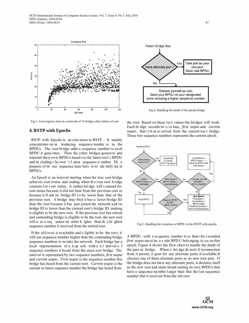
IJCSI International Journal of Computer Science Issues, Vol. 7, Issue 4, No 3, July 2010 ISSN (Online): 1694-0784 ISSN (Print): 1694-0814 47
Fig.3. Convergence time in a network of 16 bridges after failure of root
4. RSTP with Epochs
RSTP with Epochs is an exte nsion to RSTP . It mainly concentrates on in troducing sequence numbe rs in the BPDUs. The root br idge adds a sequence number to each BPDU it gene rates. Then the o ther bridges genera te and transmit their own BPDUs based on the latest root’s BPDU and in cluding t he root ’s l atest sequence n umber. Th e purpose of th ese sequence num bers is to ide ntify sta le BPDUs.
An Epoch is an interval starting when the true root bridge achieves root st atus and ending when th e t rue root b ridge contests f or r oot status. A nother bri dge will c ontend for root status because it did not hear from the previous root or because it fi nds its bridge ID t o be lower than that of the previous root. A bridge may find it has a lower bridge ID than the root because it has just joined the network and its bridge ID is lower than the current root’s bridge ID, making it eligible to be the new root. If the previous root has retired and contending bridge is eligible to be the root, the new root will u se a seq uence nu mber h igher than th e hi ghest sequence number it received from the retired root.
If the ol d ro ot is re achable and e ligible to be the roo t, it will use sequence number higher than the contending bridge sequence numbers to re-take the network. Each bridge has a local representation of a n ep och with a n i nterval o f sequence numbers it heard from the same root bridge. The interval is represented by two sequence numbers, first seqno and current seqno. First seqno is the sequence number this bridge has heard from the current root. Current seqno is the current or latest sequence number the bridge has heard from
Fig.4. Handling the death of the parent bridge
the root. Based on these two values the bridges will work. Each br idge records tw o va lues, first seqno and current seqno., that i t h as re ceived from the current roo t bridge. These two sequence numbers represents the current epoch.
Fig.5. Handling the reception of BPDU in the RSTP with epochs
A BPDU with a se quence number le ss than t he r ecorded first seqno mu st be a s tale BPD U belo nging to a n ea rlier epoch. Figure 4 shows the flow chart to handle the death of the pare nt bridge. When a bri dge de tects d isconnection from it parent, i t goes for any alternate ports if available.It chooses one of these alternate ports as its new root port. I f the bridge does not have any alternate ports, it declares itself as the new root and starts broad casting its own BPDUs that have a sequ ence nu mber l arger than that the l ast seq uence number that it received from the old root.
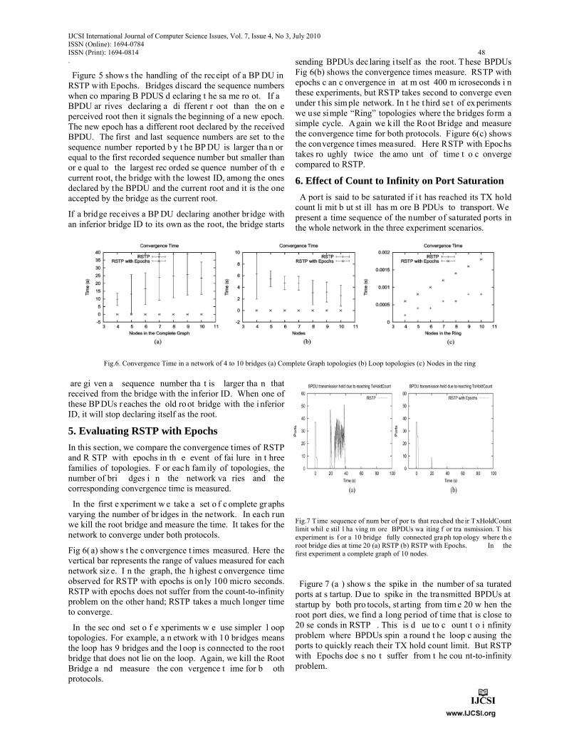
IJCSI International Journal of Computer Science Issues, Vol. 7, Issue 4, No 3, July 2010 ISSN (Online): 1694-0784 ISSN (Print): 1694-0814 48
.
Figure 5 shows the handling of the receipt of a BP DU in RSTP with Epochs. Bridges discard the sequence numbers when co mparing B PDUS d eclaring t he sa me ro ot. If a BPDU ar rives declaring a di fferent r oot than the on e perceived root then it signals the beginning of a new epoch. The new epoch has a different root declared by the received BPDU. The first and last sequence numbers are set to the sequence number reported b y t he BP DU is larger tha n or equal to the first recorded sequence number but smaller than or e qual to the largest rec orded se quence number of th e current root, the bridge with the lowest ID, among the ones declared by the BPDU and the current root and it is the one accepted by the bridge as the current root.
If a bridge receives a BP DU declaring another bridge with an inferior bridge ID to its own as the root, the bridge starts
sending BPDUs dec laring i tself as the root. These BPDUs Fig 6(b) shows the convergence times measure. RSTP with epochs c an c onvergence in at m ost 400 m icroseconds i n these experiments, but RSTP takes second to converge even under t his sim ple network. In t he t hird se t of ex periments we use simple “Ring” topologies where the bridges form a simple cycle. Again we kill the Root Bridge and measure the convergence time for both protocols. Figure 6(c) shows the convergence t imes measured. Here RSTP with Epochs takes ro ughly twice the amo unt of time t o c onverge compared to RSTP.
6. Effect of Count to Infinity on Port Saturation
A port is said to be saturated if i t has reached its TX hold count li mit b ut st ill has m ore B PDUs to transport. We present a time sequence of the number of saturated ports in the whole network in the three experiment scenarios.
Fig.6. Convergence Time in a network of 4 to 10 bridges (a) Complete Graph topologies (b) Loop topologies (c) Nodes in the ring
are gi ven a sequence number tha t is larger tha n that received from the bridge with the inferior ID. When one of these BP DUs r eaches the old ro ot bridge with the i nferior ID, it will stop declaring itself as the root.
5. Evaluating RSTP with Epochs
In this section, we compare the convergence times of RSTP and R STP with epochs in th e event of fai lure in t hree families of topologies. F or eac h fam ily of topologies, the number of bri dges i n the network va ries and the corresponding convergence time is measured.
In the first e xperiment w e take a set o f c omplete gr aphs varying the number of br idges in the network. In each run we kill the root bridge and measure the time. It takes for the network to converge under both protocols.
Fig 6( a) show s t he c onvergence t imes measured. Here the vertical bar represents the range of values measured for each network siz e. I n the graph, the h ighest c onvergence time observed for RSTP with epochs is on ly 100 micro seconds. RSTP with epochs does not suffer from the count-to-infinity problem on the other hand; RSTP takes a much longer time to converge.
In the sec ond set o f e xperiments w e use simpler l oop topologies. For example, a n etwork with 10 bridges means the loop has 9 bridges and the l oop is connected to the root bridge that does not lie on the loop. Again, we kill the Root Bridge a nd measure the con vergence t ime for b oth protocols.
Fig.7 T ime sequence of num ber of por ts that reached the ir TxHoldCount limit whil e stil l ha ving m ore BPDUs wa iting f or tra nsmission. T his experiment is f or a 10 bridge fully connected gra ph top ology where th e root bridge dies at time 20 (a) RSTP (b) RSTP with Epochs. In the first experiment a complete graph of 10 nodes.
Figure 7 (a ) show s the spike in the number of sa turated ports at s tartup. Due to spike in the transmitted BPDUs at startup by both pro tocols, st arting from tim e 20 w hen the root port dies, we find a long period of time that is close to 20 se conds in RSTP . This is d ue to c ount t o i nfinity problem where BPDUs spin a round t he loop c ausing the ports to quickly reach their TX hold count limit. But RSTP with Epochs doe s no t suffer from t he cou nt-to-infinity problem.

IJCSI International Journal of Computer Science Issues, Vol. 7, Issue 4, No 3, July 2010 ISSN (Online): 1694-0784 ISSN (Print): 1694-0814 49
Fig.8 Time s equence of num ber of ports t hat r eached the ir TxHoldCount limit whi le th ey still ha ve more BPDUs waiting for tra nsmission. This experiment is for a 10 bridge “loop” topology. The root bridge dies at time 20. (a) RSTP. (b) RSTP with Epochs.
Similarly in the second experiment, we observe from figure 8 (a) the spike in the number of satured ports at startup. We also observe in RSTP a p eriod after the fa ilure of the root bridge where there are several saturated ports. Again this is due to the count-to-infinity problem.
Fig. 9 Time sequence of number of ports reaching their TxHoldCount limit while still having more BPDUs waiting for transmission. This experiment is for a 10 bridge ring topology where a link connecting the root bridge to a neighbor dies at time 20. (a) RSTP. (b) RSTP with Epochs.
In the third experiment, failure of the root cuts the loop so there is no count t o infinity. Thus fo r bo th protocols no ports get saturated after the failure that you can see in fig.9
7. Conclusions
In stu dying R STP under pa rtial ne twork failure, it ca n exhibit a c ount-to-infinity problem. In experiments, w e observe t hat in som e scena rios the c ount to infinity ca n extend the co nvergence time t o reach 50 s econds. Du ring the count to in finity, b ridges t ransmit a lot more B PDUs than during its normal operation. In this work, we identify the e xact co nditions u nder w hich the c ount-to-infinity problem arises. We propose a simple and effective solution called RSTP with epochs that eliminate the count to infinity problem. This solution also enhances the convergence time.
References
1) “Spanning tree pro tocol probl ems and related design consideration,” Cis co sy stems, Inc. (online). www.cisco.can/ward/public/473/16.htm/
2) K. Elm eleegy, “ RSTP with E pochs simulator”, 2007 (online) http://www.cs.rice.edu/kdiaa/ethernet
3) K. Elmelegy, A . L. Cox, a nd T .S.E.Ng, “ On c ount-to-infinity induced f orwarding lo ops in Ethern et n etworks,” in P roc. IEEE Infocom 2006, Barcelona, Spain, Apr. 2006.
4) K. Elmelegy, A.L.Cax, and T.S.E.Ng, “ Etherfuse: An Ethernet watch d og,” i n P roc. A CM SIG Communications, K yoto, J apan, Aug.2007, pp. 253-264.
5) Khaled Elm eleegy, A lan L. Cox , and T. S. E ugene Ng. “Understanding and Mitigating the Effects of Count to Infinity in Ethernet Networks ”. To appear in IEEE/ACM Transactions on Networking.
6) R. Garcia, J. Duato and F.Silla “LSOM:A link state protocol over MAC addresses for metropolitan backbones using optical Ethernet switches” in proc. 2nd IEEE Int .Symp. Network Computing and Applications (NCA’03), pp.315-321, Apr.2003.
7) J. J. Gracia-lunes-Aceves, “Loop-free routing using diffusing computations,” IEEE/ACM Trans. on Networking, vol.1, No.1, pp.130-141, Feb.1993
8) J. M. Jafee and F. H. Moss, “A responsive distributed routing algorithm in computer networks,” IEEE Trans. on Communications., vol. 30, No.7, pp.1758-1767, July 1982
9)R.Pelman “RBridges:Transparent Routing,”in proc.IEEE IN-FOCOM,2004,vol.2,pp.234-244
10)S.Ray,R.A.Guerin and R.Sofia “Distributed path computation with out Transient loops” ,” IEEE Trans. on Communications., vol. 30, No.7, July
Mr. D. Ganesh received his B.Tech degree in Information Technology from JNT University, Hyderabad in 2006 and M.Tech degree in Computer Science and Engineering from Acharya Nagarjuna University in 2010.During the period 2006-07 he worked as Assistant Professor in Information Technology
department at AITS, Rajampet, India. Since 2007, he is working as Assistant Professor in IT Department at Sree Vidyanikethan Engineering College, Tirupati, India. He has Published 4 papers in national and International conferences. His current research interests are computer networks, Object oriented design and unified modeling. He is a member of ISTE, CSI
Dr. Rama Prasad V Vaddella was born in Tirupati, India in 1962. He received the M.Sc (Tech.) degree in Electronic Instrumentation from Sri Venkateswara University, Tirupati in 1986 and M.E degree in Information Systems from BITS, Pilani, India in 1991. During the period
1989-1992 he worked as Assistant Lecturer in Computer Science at BITS, Pilani. From 1992 to 1995, he worked as Lecturer in Computer Science and Engineering and as Associate Professor from 1995 to 1998 at RVR & JC College of Engineering, Guntur, India. Since 1998, he is working as Professor and Head of Information Technology department at Sree Vidyanikethan Engineering College, Tirupati, India. He was awarded the Ph.D degree in Computer Science by J.N.T. Univeristy, Hyderabad, during 2007 for his thesis in Fractal Image Compression. He is also holding the additional position of Chairman, Board of Studies in Computer Science, and Vice-Principal at Sree Vidyanikethan Engineering College (Autonomous under JNT University, Anantapur, India). He has also worked as a short time Research Assistant at Indian Institute of Science, Bangalore during the year 1986. He has published about 10 papers in national and international conferences and 05 papers in International journals, edited books, and refereed conferences. He is also a member of the editorial review board for 05 International journals in Computer Science and Information Technology. His current research interests include computer graphics, image processing, computer networks, computer architecture and neural networks. He is a member of IEEE, ISTE and CSI

IJCSI CALL FOR PAPERS JANUARY 2011 ISSUE
V o l u m e 8 , I s s u e 1
The topics suggested by this issue can be discussed in term of concepts, surveys, state of the art, research, standards, implementations, running experiments, applications, and industrial case studies. Authors are invited to submit complete unpublished papers, which are not under review in any other conference or journal in the following, but not limited to, topic areas. See authors guide for manuscript preparation and submission guidelines. Accepted papers will be published online and indexed by Google Scholar, Cornell’s University Library, DBLP, ScientificCommons, CiteSeerX, Bielefeld Academic Search Engine (BASE), SCIRUS, EBSCO, ProQuest and more. Deadline: 05th December 2010 Notification: 10th January 2011 Revision: 20th January 2011 Online Publication: 31st January 2011 Evolutionary computation Industrial systems Evolutionary computation Autonomic and autonomous systems Bio-technologies Knowledge data systems Mobile and distance education Intelligent techniques, logics, and
systems Knowledge processing Information technologies Internet and web technologies Digital information processing Cognitive science and knowledge
agent-based systems Mobility and multimedia systems Systems performance Networking and telecommunications
Software development and deployment
Knowledge virtualization Systems and networks on the chip Context-aware systems Networking technologies Security in network, systems, and
applications Knowledge for global defense Information Systems [IS] IPv6 Today - Technology and
deployment Modeling Optimization Complexity Natural Language Processing Speech Synthesis Data Mining
For more topics, please see http://www.ijcsi.org/call-for-papers.php All submitted papers will be judged based on their quality by the technical committee and reviewers. Papers that describe on-going research and experimentation are encouraged. All paper submissions will be handled electronically and detailed instructions on submission procedure are available on IJCSI website (www.IJCSI.org). For more information, please visit the journal website (www.IJCSI.org)

© IJCSI PUBLICATION 2010
www.IJCSI.org

IJCSIIJCSI
© IJCSI PUBLICATION www.IJCSI.org
The International Journal of Computer Science Issues (IJCSI) is a well‐established and notable venue
for publishing high quality research papers as recognized by various universities and international
professional bodies. IJCSI is a refereed open access international journal for publishing scientific
papers in all areas of computer science research. The purpose of establishing IJCSI is to provide
assistance in the development of science, fast operative publication and storage of materials and
results of scientific researches and representation of the scientific conception of the society.
It also provides a venue for researchers, students and professionals to submit ongoing research and
developments in these areas. Authors are encouraged to contribute to the journal by submitting
articles that illustrate new research results, projects, surveying works and industrial experiences that
describe significant advances in field of computer science.
Indexing of IJCSI 1. Google Scholar 2. Bielefeld Academic Search Engine (BASE) 3. CiteSeerX 4. SCIRUS 5. Docstoc 6. Scribd 7. Cornell's University Library 8. SciRate 9. ScientificCommons 10. DBLP 11. EBSCO 12. ProQuest


![Untitled-1 []Title Untitled-1 Author Sivaselvan R Created Date 10/17/2018 1:04:36 PM](https://static.fdocuments.in/doc/165x107/5f2c5d67ad6c2707195778d1/untitled-1-title-untitled-1-author-sivaselvan-r-created-date-10172018-10436.jpg)


![Untitled-1 [] · Title: Untitled-1 Author: Sivaselvan R Created Date: 10/16/2018 6:25:30 PM](https://static.fdocuments.in/doc/165x107/5f5f59b607d6656d324e9af0/untitled-1-title-untitled-1-author-sivaselvan-r-created-date-10162018-62530.jpg)