IIT BOMBAY NPTEL NATIONAL PROGRAMME ON TECHNOLOGY ENHANCED...
17
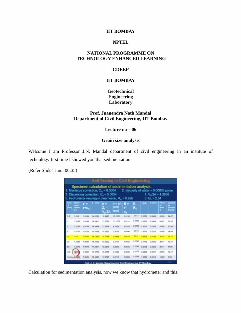
IIT BOMBAY NPTEL NATIONAL PROGRAMME ON TECHNOLOGY ENHANCED LEARNING CDEEP IIT BOMBAY Geotechnical Engineering Laboratory Prof. Jnanendra Nath Mandal Department of Civil Engineering, IIT Bombay Lecture no – 06 Grain size analysis Welcome I am Professor J.N. Mandal department of civil engineering in an institute of technology first time I showed you that sedimentation. (Refer Slide Time: 00:35) Calculation for sedimentation analysis, now we know that hydrometer and this.
Transcript of IIT BOMBAY NPTEL NATIONAL PROGRAMME ON TECHNOLOGY ENHANCED...
IIT BOMBAY
NPTEL
NATIONAL PROGRAMME ON TECHNOLOGY ENHANCED LEARNING
CDEEP
IIT BOMBAY
GeotechnicalEngineeringLaboratory
Prof. Jnanendra Nath MandalDepartment of Civil Engineering, IIT Bombay
Lecture no – 06
Grain size analysis
Welcome I am Professor J.N. Mandal department of civil engineering in an institute of
technology first time I showed you that sedimentation.
(Refer Slide Time: 00:35)
Calculation for sedimentation analysis, now we know that hydrometer and this.
(Refer Slide Time: 00:53)
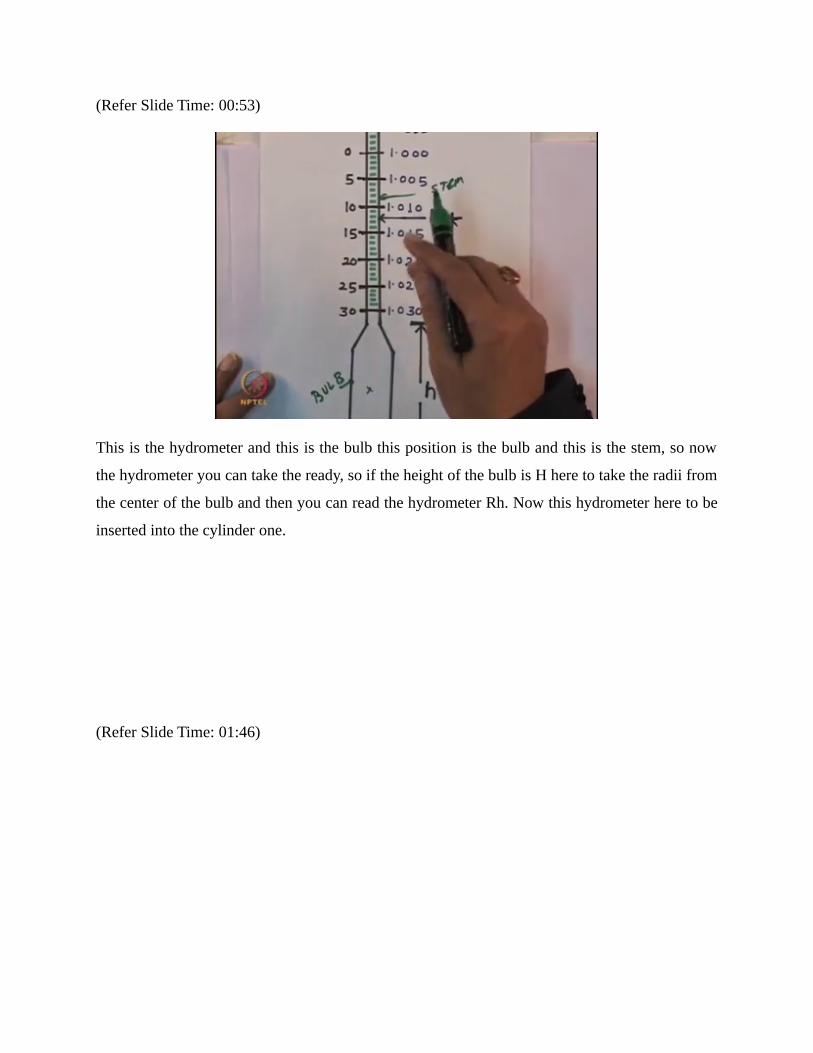
This is the hydrometer and this is the bulb this position is the bulb and this is the stem, so now
the hydrometer you can take the ready, so if the height of the bulb is H here to take the radii from
the center of the bulb and then you can read the hydrometer Rh. Now this hydrometer here to be
inserted into the cylinder one.
(Refer Slide Time: 01:46)

The image that water or the any liquid suspension will be there, so this is the hydrometer and this
hydrometer here to insert a into this cylinder in which distill water or water suspension will be
there, now we have to take the hydrometer reading this hydrometer leading you insert it and take
the hydrometer leading at total a last time of half one and two minutes without removing the
hydrometer, after the two minutes leading then remove the hydrometer this hydrometer is
remove it without disturbance the suspension and raise it in the numbering one cylinder, so
another numbering cylinder.
Is there in a distill water only should be there, this distill water so we have to press this
hydrometer into this devring cylinder continuing only distill water and rearrange it by visiting
motion this one okay, and if you want it to remove any soil particle that they have settle one it,
then the subsequent ready after the period of 5 10 15 30 60 and 120 minutes and record heat the
temperature of the soil water suspension using the thermometer and with the suspension as such
for leading to be taken after 24 hour and 48 hour.
So this the table which it has been solve that after different time, it is here different hydrometer
reading is taken under the different time so here to take the leading in different time and we have
to measure the what should be the hydrometer reading, so how can you take the hydrometer
reading we want this hydrometer reading it is necessary to calibrate the hydrometer, so how to
calibrate the hydrometer so we have calibration of hydrometer is essential, so for example that
this is the.

(Refer Slide Time: 05:21)
Hydrometer and this height of this hydrometer is 12cm, so half 0f this about 6cm and from there
it is 7cm and this hydrometer is reading 1.030 1.025 1.020 1.015 0. 010 1.005 and 1.00 and 0.995
and this turns is 2cm interval so you can take any reading of hydrometer and then we can draw
this from this height x axis this is height from the center of the bulb of the hydrometer reading
and this is the hydrometer reading, so for example that if you want to or any hydrometer reading
if you want to take at this location let us say this is 7 + 29 + 11 and then you can read the reading
1.020.
So similarly for this 11 if you go for the 11 and then we can have the hydrometer reading 1.02
like that for any location we can calculate the what will be the hydrometer reading, so this y and
this hydrometer has been calibrated and for the define hydrometer you can have the different
types of the calibration chart. So this is important and then you can take the reading and can
determine that what will be the reading for the hydrometer, now how to calculate the meniscus
correction so here.
(Refer Slide Time: 07:31)
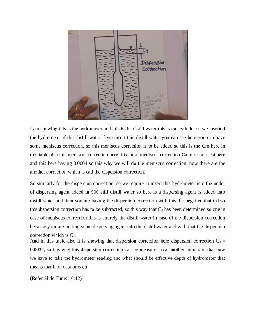
I am showing this is the hydrometer and this is the distill water this is the cylinder so we inserted
the hydrometer if this distill water if we insert this distill water you can see here you can have
some meniscus correction, so this meniscus correction is to be added so this is the Cm here in
this table also this meniscus correction here it is these meniscus correction Ca in reason test here
and this here having 0.0004 so this why we will do the meniscus correction, now there are the
another correction which is call the dispersion correction.
So similarly for the dispersion correction, so we require to insert this hydrometer into the under
of dispersing agent added in 900 still distill water so here is a dispersing agent is added into
distill water and then you are having the dispersion correction with this the negative that Cd so
this dispersion correction has to be subtracted, so this way that Cd has been determined so one in
case of meniscus correction this is entirely the distill water in case of the dispersion correction
because your are putting some dispersing agent into the distill water and with that the dispersion
correction which is Cd.And in this table also it is showing that dispersion correction here dispersion correction C d =
0.0034, so this why this dispersion correction can be measure, now another important that how
we have to take the hydrometer reading and what should be effective depth of hydrometer that
means that h on data or each.
(Refer Slide Time: 10:12)

So this is the cylinder and this the suspension liquid then you are inserting the hydrometer into
the suspension liquid, now initially the hydrometer or now when you insert the hydrometer into
the suspension liquid then it up and this balloon from here to here this balloon will be Vh / A this
is balloon of hydrometer and this is cross sectional area and in the bulb this will be Vh / 2A so if
the initial position is here to here then final position is b into b1 a1 to a1, so this distance is equal
to h and this distance is equal to h/2.
And this is Vh/ 2 so this is due to the effect of the hydrometer inversion then how you calculate
the hydrometer is and how you take the reading for Rh now this sedimentation just before the
insertion of the hydrometer is in this location, so here to calculate what will be the effective
height that means He or data okay. So this height He will be equal to from here to here is Vh / A
and this distance is equal to H and this distance us h/2 and this is Vh/2A, so what we can write
from here.
(Refer Slide Time: 12:23)

That H of e will be equal to H + h/2 + Vh/2 of A this – Vh / A that means this will be H + ½ of h
– Vh / A, so you can calculate the effective depth H of e with this equation so this is constant half
because this is hydrometer bulb this is almost the hydrometer and this is cross sectional area so
this is constant so this can.
(Refer Slide Time: 13:21)
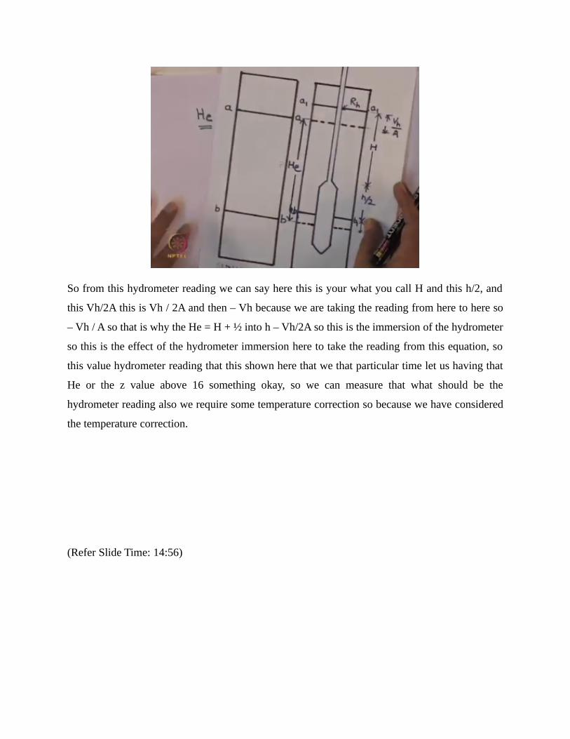
So from this hydrometer reading we can say here this is your what you call H and this h/2, and
this Vh/2A this is Vh / 2A and then – Vh because we are taking the reading from here to here so
– Vh / A so that is why the He = H + ½ into h – Vh/2A so this is the immersion of the hydrometer
so this is the effect of the hydrometer immersion here to take the reading from this equation, so
this value hydrometer reading that this shown here that we that particular time let us having that
He or the z value above 16 something okay, so we can measure that what should be the
hydrometer reading also we require some temperature correction so because we have considered
the temperature correction.
(Refer Slide Time: 14:56)

Or we can determine that viscosity of water at different temperature so if the temperature is just
280C and then viscosity of water 10.008360 and this viscosity I can also show you later that this
value has been added, so viscosity is added that is equal to η and that depend upon what will be
the temperature because if we insert the for meter into the suspension liquid and take the
measurement of the temperature and you can add if is more than 270C or if it is less the we can
subtractive.
So you can do all the correction that means we required for the meniscus correction we require
for the dispersion correction will measure the a temperature and you determine what should be
the viscosity of the water okay , and that particular temperature now here to calculate that what
should be the H that is z / Vh / 2 here and then that you can calculate for a particular time so we
can calculate that h, now we have to calculate that t that us H / t that is cm / m, so this can be.
(Refer Slide Time: 16:55)

That this can be calculated that is h/t and here h / z value here calculating here this value we are
calculating so we know that what is h that is h this V okay this is B value we know that what is
the h, we know that what is the time so we can calculate the V/h so V/h is equal to h = 14.7718
and this divided by that is 15 minutes time so this will be above 0.9847, so this is the V so here
that v is showing above 0.98, now we have to correct the applying the dispersion correction in
for dispersion correction.
So dispersion correction we say R = 1.0104 – 0.0034 so this will be 1.0070 because that
dispersion corrections here we given 0.0034 so here that here the dispersion correction is 00C4
so it can be that 0034and so R will be equal to 1.0014 that means whatever the reading we have
taken here 1.0 0.04 and – this dispersion correction that is basic Cd so align the dispersion
correction, so we can correct this dispersion correction now we have to calculate what should be
the vertical diameter that is.
So this dispersion correction then also we can calculate that what will be the R value also that
water value is this one that is that Rw = 0.996 so this Re – Rw is 0.0016 now we have calculate
this particle diameter that d so particle diameter particle diameter d.(Refer Slide Time: 20:09)
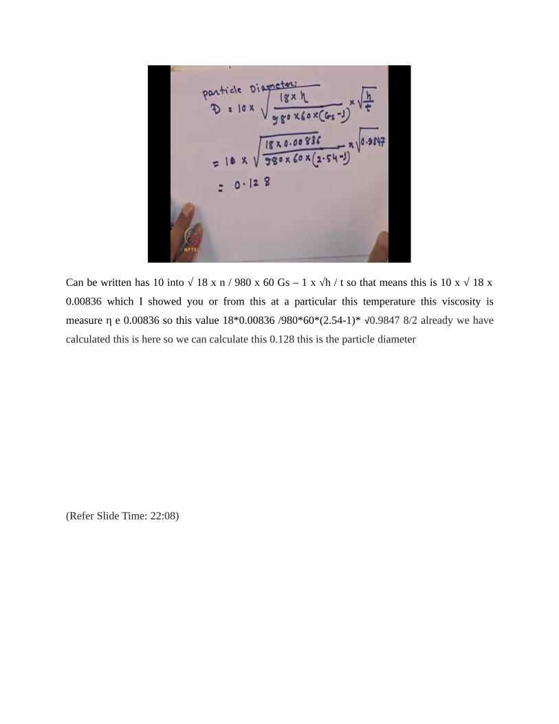
Can be written has 10 into √ 18 x n / 980 x 60 Gs – 1 x √h / t so that means this is 10 x √ 18 x
0.00836 which I showed you or from this at a particular this temperature this viscosity is
measure η e 0.00836 so this value 18*0.00836 /980*60*(2.54-1)* √0.9847 8/2 already we have
calculated this is here so we can calculate this 0.128 this is the particle diameter
(Refer Slide Time: 22:08)

Then we can calculate particle diameter this will be correlate diameter is 0.01 and 0.128 this
particle diameter is shown now we have to calculate the percent fimer now we have calculate the
percent fimer that means percentage fimer is diginitive at them. So percent fimer so this percent
from the N= Gs/Gs-1 *Vs/Ws*(R-Rw)*100.
So you know that Gs is 2.54 /2.54-1*1000 and this divide by 52.8*R value as Rw values also we
called as also recorded this is the area we can nearly we can take that Rw value this I R and this
R- Rw and Rw value is given 0.96 so this is R-Rw value so this is R this is Rw value. So you can
write this 1. 007-0.996 * 100 for this we can determine that should be the in value at the 34.35.
(Refer Slide Time: 24:41)

So you have to type the N'= N*N's /100 so this N value 34.35 which we have 45.7 s divided by
100. So this 15.7 so this in the N value as 16.70 this shows that I am showing that 1 of the
particular time it will we can calculate the what should be the effective correlation and we can
calculate by the data by the age per year we can calculate the V and we can calculate R then R-
Rw and then this diameter.
(Refer Slide Time: 27:01)

So for the different line that we are calculating and it note that percent diameter also so how this
table now from this table you can draw what will be the this side of the density so Gensen
distribution curve it like this and this part is for the glummer analysis and this part for the sand
analysis and then this part is for the hybrid ten analysis.
So this is the relationship between the grain size of this axis in millimeter giving in the side and
this is the final percentage so how this relation curve is knowing that percentage that travel and
what percentage of the sand is there in this side sample so this gradation curve is very important.
(Refer Slide Time: 28:38)

So how this gradation curve we can determine from the different parameters and some of the
parameters is called that effective size is equal to D10 we can calculate that uniformity that
coefficient and μ is equal to D60/ D10. We can calculate also the coefficient of curvature and that
is D302/ D10*D60.
So how this gradation curve it can calculate 60% of this or 40% of this curve and 10% of the
curve this is the detail and then you have to see the value will be here then we can calculate that
what will be a correlation and what will be the curvature.
(Refer Slide Time: 29:58)

And also from this part we can also calculate that what should be the double so this double
percentage so as well gravel 4.75mm and above and at the sand 0.075mm to 4.75mm and for the
silt this is 0.075mm to 0.002 mm and clay as 2 micro that is 0.002mm and less. And you have
these derivations so you can determine what is the percentage of gravel sand clay from this
derivation. Thank you
NPTELPrincipal Investigator
IIT Bombay
Prof. R. K. Shevgaonkar
Head CDEEPProf. V. M. Gadre
ProducerArun Kalwankar
Online Editor& Digital Video EditorTushar Deshpande
Digital Video Cameraman& Graphic DesignerAmin B Shaikh
Jr. Technical AssistantVijay Kedare

Teaching AssistantsAnkita KumarSunil Ahiwar
Maheboobsab NadafAditya Bhoi
Sr. Web DesignerBharathi Sakpal
Research AssistantRiya Surange
Sr. Web DesignerBharati M. Sarang
Web DesignerNisha Thakur
Project AttendantRavi PaswanVinayak Raut
MusicStandard Sandwich- by smilingcynic
Copyright NPTEL CDEEP IIT Bombay