DRAFT

Physics of Condensed States

Chapter I-A:

INTRODUCTION

by

Steven A. Kivelson and Aharon KapitulnikSTANFORD UNIVERSITY,

Stanford, CA 94305

March 30, 2015

Preface - how to read this chapter

In this section, we will take a first, broad-brush look at the physics of solids, with-out much explicit detail or analysis. The purpose of this exercise is to familiarizeourselves with the sort of phenomena we are trying to understand, and to orientourselves concerning the conceptual approach we are going to adopt. If you have nothad any introduction to solid state physics, some (hopefully not many) of the termswill be unfamiliar, but these will all be studied in detail in subsequent chapters. Ifcertain declarative statements seem outrageously general and strong, try to preservethat sense of outrage so that, when you read the appropriate later section where theresults are derived, you will be amazed and delighted (as opposed to bored and an-noyed) by the power and simplicity of the arguments that underlie these conclusions.It may also be useful to the student to come back and reread this section, at theend of the course of study; it is hoped that, armed with somewhat more understand-ing, this section will serve the secondary purpose of summarizing the most salientwell understood features of the subject and indicating directions in which significantunknowns may lie.

1

Looking at tables is not, generally, one of the most exciting of undertakings.Nevertheless, try to look at the numbers we have assembled below with wonderand astonishment. These represent the real, experimentally measured properties ofsolids. It is an essential feature of this field that these numbers can be tabulated atall. In the middle ages, for example, metallurgy was such a mysterious subject thatwhen, accidentally, due to the skill and luck of the smith, a particularly good steel wasproduced and forged into a sword, that sword became the center of enduring legends.Nowadays, we have, for the most part, mastered the science of making materials withextraordinary levels of purity, growing crystals with remarkable degrees of perfection,in short, making materials with properties that can be tabulated. It is the legacy ofthese accomplishments of materials science that permits you to contemplate thesetabulated results.

1 Condensed Matter Theory

Because condensed matter is so complicated, it follows that any attempt to directlyconfront the problem by simply solving the Schrodinger equation is doomed to rely ona series of uncontrolled approximations. Thus, it is necessary to have some guidingprinciples that allow one to interpret the relevance to real materials of the results ofthe rather simple calculations we are able to carry out. Fortunately, in many cases,this is possible. Indeed, it is a remarkable but demonstrably true statement that,at least in the best cases, one can actually understand many properties of materialsqualitatively, and in some fortunate circumstances even quantitatively, in terms ofrather simple considerations.

It is an empirical fact that, in many cases, different solids exhibit broadly similarbehavior. Cu, Fe, and Pb are all “metals” at room temperature. This is not justa name, but a category, which reflects the fact that there is considerable similar-ity in their properties. Each of them is a good conductor of electricity and heat,their specific heats are of comparable magnitudes and, at low temperatures, areproportional to temperature to the first power, and they all have a more or lesstemperature independent paramagnetic susceptibility, etc. Moreover, the same istrue, with various caveats, of all sorts of more complicated metals, including variouscomplex alloys. Now each of these materials is the name of a completely differentHamiltonian. What we learn from this is that, in many respects, the “answer”, thatis to say the macroscopic observable physical characteristics of a condensed matersystem, is often broadly independent of the “question”, that is to say the microscopicHamiltonian that determines the dynamics and the thermodynamics of the problemin question. Clearly, if that is true of a broad class of physical Hamiltonians, it mustbe true of a broad class of unphysical ones as well.

This notion suggests an effective strategy for approaching condensed matter

2

physics: We will solve various very simple model problems (e.g. model Hamil-tonians). Of course, we will be guided by physical principles in defining our models,so that as much as possible each simple model incorporates the important physicsof interesting materials. And we will develop methods for systematically improvingour results in the sense that we will learn to incorporate some of the details thatactually differentiate one metal from another, or one insulator from another. Butthe basic idea is that it is more illuminating to solve a very simple model correctly,than to solve a “realistic” model crudely.

This is not the only approach that has been taken to the study of condensedmatter. There has been a concerted and remarkably successful effort to computethe properties of solids from “first principles”, i.e. from the Schrodinger Equation.This approach is similar in spirit to various “ab initio” approaches to the quantumchemistry of molecules. The disadvantages of this approach are that the methodol-ogy necessarily involves some theoretically uncontrolled, albeit physically motivatedapproximations, the calculations tend to be computationally intensive, and the an-swers tend to be quite complex. It is largely for the latter reasons that this ”firstprinciples band-structure” approach is treated relatively briefly and incompletely inthe present text – the student who is interested in a more detailed introduction tothis approach might wish to consult Refs. [1] and [2].1

We will ultimately need a better justification for our approach than “If naturecan solve different models and get the same physics, why can’t we?” We will need tounderstand: When does this work? For what class of properties does it work? Howaccurately does it work? For a given material, is there a way to derive the simplesteffective model that captures the relevant macroscopic physics?

1.1 Emergence and Adiabatic Continuity

The notion that the macroscopic behavior of a complex system is insensitive to manyfeatures of the microscopic dynamics is an example of “emergence.” In the “reduc-tionist” approach, all of condensed matter physics is implicit in the Schrodingerequation (or, if relativistic effects are important, the Dirac equation), and so con-densed matter theory is an exercise in applied quantum mechanics. However, in areal sense, the emergent character of macroscopic phenomena is at odds with thereductionist viewpoint, and leads one to consider the collective properties of matteras fundamentally new and distinct from the microscopic. The philosophical implica-tions of this observations have been discussed in a number of books and monographs,of which two of the most accessible and influential are Refs. [1] and [2].2

11) W. A. Harrison, “Elementary Electronic Structure,” 2) D. A. Papaconstantopoulos, “Hand-book of the Band Structure of Elemental Solids.”

21) P.W. Anderson, “More is different,” 2) R. B. Laughlin, “A different Universe.”

3

More formally, the basic reason we believe that simple models capture the essenceof reality derives from the concept of adiabatic continuity in thermodynamics. Withina given thermodynamic phase, thermodynamic quantities are analytic functions ofthe externally controlled parameters. Thermodynamic quantities include the freeenergy and its various derivatives, e.g. the specific heat, and also various thermody-namic correlation functions. Non-analyticities only occur across phase boundaries,where the thermodynamic phase of the system changes. Note that as we change cer-tain familiar thermodynamic variables, such as the volume and the magnetic field, weare changing the Hamiltonian of the system, so this is a precise statement concerningthe robustness of the macroscopic physics to changes in the Hamiltonian.

This invites us to consider a large space - the space of all possible many-bodyHamiltonians, and to think of the phase diagram of all possible condensed matter inthis large space. Then, for all systems described by Hamiltonians in a given “phase”,the analytic forms of various important quantities are the same.

These notions from thermodynamics help us further refine our notion of the use-fulness of models. Because of the analyticity property, two microscopic Hamiltoniansdescribing the same phase will produce qualitatively similar macroscopic physics.Moreover, if we can compute the thermodynamic properties of a model Hamiltonianwhich is “near” to the Hamiltonian of a physical system of interest, then we can re-fine our results by treating the difference between the physical Hamiltonian and themodel Hamiltonian with perturbation theory. (Analytic functions can be expandedin a power series, thus justifying perturbation theory.)

1.2 Effective Field Theories and the Renormalization Group

All equilibrium properties of a system can, in principle, be derived from the partitionfunction

Z = Tre−βH

(1)

where the trace is performed on all possible states of the system. The free energy isrelated to the partition function as

F = −T ln[Z] (2)

and all thermodynamic correlation functions (which can also be thought of as par-ticular derivatives of the partition function) can be computed as

〈O〉 = Z−1Tre−βHO

(3)

where O is any physical observable.Of course, performing these calculations explicitly is prohibitively difficult. What

we are always interested in is the simplest possible approximate evaluation of these

4

quantities. In attempting this, we will focus on “effective” models of condensedmatter systems - which are generalized versions of “effective field theories.” Formally,one imagines first doing partial traces in evaluating the thermodynamics properties ofa system, in which we “integrate out” the high energy degrees of freedom, leaving uswith a theory expressed only in terms of a smaller number of important (low energy)degrees of freedom with effective interactions that are generated in the process. (Aprecise definition of a procedure to integrating out degrees of freedom is presented inAppendix A.) For instance, we rarely concern ourselves explicitly with the behaviorof the core electrons which are tightly bound to the nuclei, and we never concernourselves with the dynamics of the nucleons within the nucleus. In the case ofthe nucleons, there is a large separation of energy scales which makes the effect ofintegrating out these degrees of freedom easy to deduce. However, typically theeffective interactions generated when integrating out high energy modes would be socomplicated that we would be unable to even understand what they mean.

Two observations make this problem somewhat less vexing than it seems at first:Deep in a phase, the system is typically insensitive to small changes, so we can hopeto obtain a valid description of the properties of such a system even if the effectivetheory we are studying is somewhat crude. Conversely, if we study the propertiesof a system “close” to a critical point, where the correlation lengths are long andhence the “microscopic details” are averaged over, the “renormalization group,” inprinciple, gives us a prescription for constructing an effective field theory in whichthere are only a relatively small number of “relevant” interactions. Invoking themagic of adiabatic continuity, we can infer properties of a given phase of mattereven if, formally, our solution applies only quantitatively in a near critical regime.

We will rarely refer to any of this aspect of the analysis as we study the propertiesof one effective model or the other. We will not explicitly introduce the renormal-ization group at all. (A fine introduction to the renormalization group as appliedto condensed matter systems can be found in Chapter 5 of Chaikin and Lubensky.)However, this circle of ideas underlies everything we will discuss; it allows the equi-librium and near equilibrium behaviors exhibited by condensed matter systems to bestudied from a single, unified perspective, and to optimally apply insights obtainedin the study of any one problem in the widest possible array of related contexts.

2 Phases of matter

One of the most important goals of condensed matter physics is to identify distinctphases of matter. Distinct phases can be identified in various ways, which we willexpand upon below. In going from one phase to another as a function of a controlparameter such as temperature (T ) or magnetic field (H), one must pass throughone or more thermodynamically special points at which a phase transition occurs.

5

A host of special physical properties characterize systems in the neighborhood of a“critical point,” i.e. the point of a phase transition.

One of the most important ways of distinguishing phases is by different patternsof spontaneously broken symmetries: Two states with different patterns of unbrokensymmetry cannot be continuously transformed into each other – as a parameter isvaried, there always must occur a first point at which the pattern of unbroken sym-metries of the system changes. Given that at high temperatures, the magnetizationof any material vanishes, for a ferromagnet there must be a unique critical tempera-ture, known as the Currie temperature TC , above which the magnetization vanishesand below which it is non-zero.

A given phase can also be characterized by the asymptotic form of various ther-modynamic correlation functions or even the asymptotic form of dynamical responsefunctions such as the conductivity tensor.3 There are also still more subtle ways thatphases, especially quantum phases in the limit T → 0, can be unambiguously dis-tinguished. Quite recently, it has come to be recognized that phases can differ inways that are not observable in any local measurement – in a still incompletely un-derstood fashion, such phases can be distinguished according to the values of certaintopological invariants. In a metal, we will see that it is also possible to distinguishphases according to the number and topology of the Fermi surface sheets.

There are many qualitative aspects of the properties of solids that depend onlyon the phase of matter involved, and not on any details. We will spend some timeunderstanding the properties of “metals,” “superconductors,” “insulators,” “ferro-magnets,” etc. All these are names of phases of matter, and by understand we meanunderstand generic physical properties that are more or less common to all matterin a given phase. However, appealing as it is to revel in the conceptual precisionwith which phases of matter can be classified, it is important to remember that inthe real world, numbers matter – two materials can be characterized as being in thesame state of matter, and yet be entirely different due to quantitative distinctions.

The importance of quantitative distinctions can be well illustrated by consideringthe difference between liquids and gases. It is somewhat embarrassing that thetechnical definition of distinct phases of matter we have given is inconsistent with themost common usage of the term – taught (properly) in all elementary school scienceclasses. Everyone knows that there are three (or four) basic states of matter: solids,liquids, gases (and, in some classes, plasmas). Solids, we teach our third graders, at agiven temperature and pressure, have a fixed volume and shape. Liquids have a fixedvolume, but take the shape of the container in which they reside. Gases expand to fillwhatever container they occupy. Plasmas, if they are included, are described as being

3As a general proposition in statistical mechanics, this statement is somewhat ambiguous withouta clear definition of what constitutes sufficiently “different” asymptotic behavior to insure that twophases are distinct.

6

sort of like gases only much hotter and better conductors of electricity. Accordingto our definition of what constitutes a phase of matter, among these four putativephases there are actually only two that are distinct – solids and fluids. The factthat solids can support a shear stress (the technical version of maintain their shape)can be used as a defining feature which permits an unambiguous distinction betweensolids and liquids. However, simple liquids and gases (and plasmas) all respect thesymmetries of space-time and have the ability to flow. No sharp distinction can bemade between them.

For example, as can be seen from the phase diagram of water shown in Fig. 1,at ambient pressure, the transition from liquid water to gaseous steam occurs by aphase transition at a sharply defined critical temperature – the boiling temperature,Tboil. However, it is possible to evolve between these two states smoothly by firstsubjecting the liquid water to high pressure, then heating it up to T > Tboil, andfinally releasing the pressure – in this way, the liquid is turned into a gas withoutsuffering a phase transition. What this means is that there is no point in the secondhistory at which one can say – before this point we were dealing with a liquid andafterwards we had a gas.

What is wrong with the elementary school discussion? The convincing soundingstatement about the constant volume occupied by a liquid is not, in fact, a descriptionof any single phase of matter, but rather refers to a state of two-phase coexistence.Because at any T > 0, the vapor-pressure of a liquid is non-zero, when we observethat only a fixed portion of a container is occupied by the liquid, we have neglectedto note that the remainder of the container is filled with the gas-form of the samematerial. Because the vapor pressure of typical liquids is so low, the fraction of thematter that is converted into gas to fill any normal size container is small comparedto the liquid fraction, so it appears that the liquid maintains its volume, independentof the size of the container. However, a very accurate measurement would reveal thatthe volume occupied by the liquid portion of a given quantity of liquid decreases withincreasing size of the container.

Liquids and gases are not distinct states of matter. However, anyone who tellsyou that this means that they are the same in all important ways, has been livingin an ivory tower for much too long!

2.1 Broken symmetries

Spontaneous symmetry breaking is one of the most dramatic emergent propertiesexhibited by condensed matter systems. The principle can be understood mostsimply by considering the example of ferromagnetism. From the fact that a magneticmoment, M, is generated by a circulating current which changes sign under timereversal, it follows that any system that is time-reversal invariant must have zeromoment. Generally, in the absence of an externally applied magnetic field, H=0,

7

the thermodynamic ensemble for any finite system is time-reversal invariant, fromwhich it follows that the equilibrium value 〈M〉=0. However, in the thermodynamiclimit (in which the size of the system L → ∞, this simple argument breaks-down.Indeed, we know that below its critical “Currie temperature,” TC , a ferromagnetretains a non-zero magnetization, even in the absence of an externally applied field.

Define m(r) to be the local magnetization density, and

M(L,H) = L−d∫Vm(r)ddr (4)

to be the magnetization per unit volume V = Ld of a system of size L (in d-dimensions) in the presence of a magnetic field, H = He, where e is a unit vector.Time reversal symmetry implies that

limH→0

M(L,H) = 0. (5)

However, again remembering our elementary school science classes, we know that ifwe take a piece of iron, heat it up, apply a magnetic field, and then cool it to roomtemperature, it retains a net magnetic moment even when the field is removed. Forall practical purposes, that piece of iron is infinite. Formally, this same physicalprinciple corresponds to the following order of limits: Let

M(H) ≡ limL→∞

M(L,H) and (6a)

M ≡ limH→0

M(H) (6b)

In the absence of spin-orbit coupling, the magnitude of M is independent of thedirection of H (i.e. e), but more generally, both the direction and magnitude of Mmay depend on e. For present purposes, the important point is that a sharp dis-tinction exists between a ferromagnetic phase, where |M| > 0, and a normal phase,in which |M| = 0. On first encounter, it may seem strange, given the validity ofEq. 5, that a ferromagnetic phase exists. However, as we shall see, the existence offerromagnetism as a representative example of a phase with a spontaneously brokensymmetry is something that we will understand well, although there are many quan-titative aspects of ferromagnetism in iron, in particular, that remain mysterious. Forthe present, we can simply take Eq. 6b to be the definition of ferromagnetism, and,by extension, of states with broken symmetry.

A broken symmetry state can also be identified by looking at the assymptoticform of a symmetry-preserving thermodynamic correlation function. For instance,we can define broken symmetries in terms of the asymptotic behavior of the two-pointcorrelation function,

〈m(r) ·m(r′)〉 → 〈m(r)〉 · 〈m(r′)〉 as |~r − ~r′| → ∞. (7)

8

In a phase without broken time-reversal symmetry, 〈m(r)〉 = 0, while in a ferromag-net, 〈m(r)〉 is non-zero and is a close relative of M, defined above. (Ppecifically,|〈m(r)〉| = |M|.) The advantage of this second definition is that it does not involveany subtle order of limits, although it is not as intuitively physical. The two defini-tions of broken symmetry can be proven[?] to be equivalent under broad conditions.

While the notion of spontaneously broken symmetry may sound abstract, we willsee that it is one of the most powerful notions in condensed matter physics. Manyproperties of a broken symmetry phase can be deduced from symmetry considera-tions, alone, without any reference to microscopic details.

2.2 Asymptotic forms of correlation functions

A system in thermal equilibrium is described by a thermal ensemble. While differentmembers of the ensemble correspond to different states of the system, intensiveproperties of the system take on a value which is equal to its mean value with aprobability that approaches unity in the thermodynamic limit. This is why, whenwe compute the mean magnetization in a ferromagnet in Eq. 4, we know that this isthe value that will be observed in an experiment in the limit that the volume, V →∞.However, this does not mean that local values of various physical observables do notvary from place to place. The extent to which such fluctuations occur is encodedin thermodynamic correlation functions, of the sort we have already encountered inEq. 7.

Typically, in a phase lacking magnetic order, such fluctuations are short-rangecorrelated, e.g. the magnetization two-point correlation function decays exponen-tially,

〈m(r) ·m(r′)〉 ∼ r−αde−|r−r′|/ξ as |r− r′| → ∞. (8)

where ξ is an associated correlation length and αd, as we shall see, is related to thespatial dimension d according to αd = (d − 1)/2. As parameters are changed, thevalue of ξ can change without it denoting a phase transition, so long as the asymptoticform of all correlation functions is preserved. At separations small compared to ξ,the system has “short-range order” which is vaguely similar to that in the brokensymmetry state, but the fluctuations about the mean are uncorrelated at two farseparated points in space.

By contrast, a state is said to have “long-range order” when a density whichshould have a vanishing average value in any symmetry preserving state, has a cor-relation function which approaches a non-vanishing value at large distances, as inEq. 7. Long-range order and broken symmetry are synonymous.

However, sometimes two-point correlation functions have a form intermediatebetween long- and short-range-order, for instance

〈m(r) ·m(r′)〉 ∼ |r− r′|−α as |r− r′| → ∞. (9)

9

where the exponent α > 0. This occurs at certain types of critical points at whicha phase transition occurs between two distinct phases of matter, in which case αtakes on certain “universal” values, which are insensitive to most microscopic details.Understanding the origin of these universal critical exponents is one of the greatintellectual accomplishments of our field.

There are also phases of matter in which such power-law correlations occur. Some-times where this occurs, the exponent α varies continuously with parameters, andso it is the existence of power-law correlations which characterizes the phase, ratherthan the value of α; such phases are often referred to as “critical phases” becausethe correlations resemble those at ordinary critical points, and they are said to have“quasi-long-range-order.” In other cases, the phase is characterized by a set of uniqueexponents, and any change in exponent would signify the existence of a new phaseof matter. We will encounter examples of both types of phases: a two-dimensionalcrystal is an example of a critical phase with quasi-long-range order, and an ordi-nary metal (technically, a “Fermi liquid”) has power-law correlations with exponentsdependent only on the spatial dimension.

Despite the “dynamics” in thermodynamics, a system in thermal equilibrium isin a time independent ensemble - the equilibrium state is unchanging as a functionof time. None-the-less, the microscopic degrees of freedom are in constant motion, sodynamic correlation functions are also of fundamental interest. This is particularlytrue in quantum systems, where the dynamics and the thermodynamics are inextri-cably intertwined due to the non-commutativity of position and momentum. Thespace and time dependence of the magnetization density, for instance, is reflected inthe dynamical two-point correlation function,

G(r, r′, t− t′) = 〈m(r, t) ·m(r′, t′)〉 (10)

where the fact that G depends only on the time interval, t − t′, and not on t andt′ separately, stems directly from the time translation invariance of the equilibriumensemble. In some cases, it will be useful to distinguish phases according to theasymptotic behavior of dynamical correlation functions as |t− t′| → ∞.

2.3 Topological and other subtle forms of order

Increasingly, in recent years, there has been excitement concerning sharply defineddistinctions between phases of matter that cannot be distinguished by measurementsof any local observable quantity. Indeed, surprising as this may sound, there is stillnot a complete theory of the subtle ways that phases, especially quantum phases atT = 0, can be distinguished.

One idea which arose only following the discovery of the fractional quantum Halleffect is that some phases can be classified by topological invariants which depend

10

only on the global properties of the system in a closed geometry. This rather abstractand seemingly physically inaccessible notion turns out to have concrete implicationsfor measurable properties. Surprisingly, it has also been realized that superconduc-tors, which in most previous text books are presented as a canonical example of astate of broken symmetry, are instead more correctly classified in a gauge invariantmanner as being “topologically ordered.” (By contrast, superfluids are correctlycharacterized as broken symmetry states.) A very recent discovery which has gener-ated enormous theoretical and experimental activity is that there exist “topologicalinsulators” which are distinct phases from ordinary insulators. Still more exoticphases, known as topological spin-liquids, have now been well characterized theoret-ically although, despite the discovery of a number of attractive “candidate” materials,the search for an unambiguous experimental realization has remained frustratinglyinconclusive.

A host of other subtle distinctions can exist between phases. One example whichwe will encounter is a distinction between different metallic phases based on thetopology of their Fermi surfaces, where here the topological character of the state isentirely different from that involved in the topological order we have just discussed.All these subtle more subtle distinctions between quantum phases of matter cannotbe understood readily on the basis of intuitions developed by every-day observationsof the properties of matter in our environment – this is something really new thatthe reader will learn about in the course of the text.

2.4 Discontinuous and continuous phase transitions and crossovers

Abstractly, a phase transition is a point at which thermodynamic functions, in par-ticular the free energy, F , have a non-analtyic dependence on a control parameter.Phase transitions are classified as “discontinuous” (or “first-order”) if there is a dis-continuity in the first derivatives of F , for instance if there is a discontinuity in theinternal energy U = T∂F/∂T . Transitions are called “continuous” if all the firstderivatives of F are continuous.

The existence and character of first order transitions is straightforward to under-stand. If there are two possible phases of a given system, then the free energy Fj(x)of each phase as a function of a control parameter x is expected to be a smooth andanalytic function of x, where j = 1 or 2 for the two phases. A transition occurs if forsome range of x, say x < xc, the system is in phase 1, i.e. F1(x) < F2(x), while forx > xc the reverse is true. Necessarily, this implies that F1(xc) = F2(xc). Becausetwo continuous curves generically cross only at isolated points, we understand whycritical points are “points.” However, there is no reason for there to be any particu-lar relation between the slopes of two curves at a point of intersection, so genericallywe would expect ∂F1(xc)/∂xc > ∂F2(xc)/∂xc. Moreover, we can see that, as far asphase 1 is concerned, there is nothing special about the value x = xc, although this

11

happens to be the point at which the two free energy curves cross. What we concludefrom this is that there should be no particular precursor effects upon the approachto a first order phase boundary – rather, the system should change suddenly fromhaving generic properties of phase 1 to generic properties of phase 2 as x is variedfrom just a bit smaller than xc to just a bit larger.

From this discussion, it would seem that continuous phase transitions would re-quire fine tuning – in order for the first derivative to be continuous across the tran-sition, it must be simultaneously true that F1(xc) = F2(xc) and ∂F1(xc)/∂xc =∂F2(xc)/∂xc. A transition which satisfies this condition, but has singularities in thesecond derivatives is called “second-order.” We will even encounter “infinite order”transitions in which all derivatives of F are continuous across the transition. Inorder for a transition to be continuous, something special must occur in the phaseas we approach the point of the phase transition which makes the two phases oneither side of the transition look increasingly like each other. Upon approaching acontinuous phase transition from x < xc there is generically a growing “correlationlength” ξ0(x) in the system, such that at distance scales large compared to ξ0, wecan clearly identify the properties of the system as being associated with phase 1,but for distance scales smaller than ξ0, the system appears “critical,” that is at hasproperties that cannot be associated with either phase 1 or phase 2, but are ratherproperties of the system at the critical point. Among other things, this requires thatξ0(x)→∞ as x→ xc.

Although critical points form a set of measure zero in the phase diagrams ofcondensed matter systems, the physics of continuous phase transitions plays an im-portant conceptual role in our understanding of the properties of solids. In general,the asymptotic long-distance properties of condensed matter systems are those ofone phase of matter or another. However, in a range of parameters sufficiently neara critical point, the properties of the system over a broad range of intermediate scalesis entirely different from that of any stable phase of matter.

2.5 Linear response and hydrodynamics

When we talk about the physical properties of a phase, we are primarily referring tothe equilibrium properties, which is to say the free energy (as a function of variousmacroscopic control parameters) and the equilibrium correlation functions alreadydiscussed. However, it turns out that many of the same considerations can be appliedto an understanding of the near equilibrium properties of materials. For example,according to Ohm’s law, when we apply an electric field E to a solid, a current jflows which is proportional to it:

jα =∑β

σαβEβ (11)

12

where the conductivity tensor, σαβ, is a characteristic feature of the material. Clearly,the ohmic current is a property of a non-equilibrium state of the system, in whichheat is being dissipated in the system at a rate per unit volume P = j ·E. However,implicit in Ohm’s law is the notion that the system is nearly in equilibrium, in thesense that the deviation from equilibrium is linear in the applied electric field. Thisis implicitly an expression that is valid only in the limit of weak applied fields; in thepresence of a large enough applied field, a huge current will flow, and so much heatwill be generated that the piece of solid will vaporize – that is not a linear response!

Ohm’s law is the most familiar of a class of relations in solids known as linearresponse. Here, we consider perturbing a system in equilibrium with a weak externalperturbation Aext(r, t) (which in general can be both a function of position and oftime), and measuring the changes in the properties of the system that are producedby this perturbation. If the perturbation is sufficiently weak, the changes or “re-sponse” of the system, R(r, t) will be approximately a linear function of the externalperturbation. Since the response of typical systems is non-local in both space andtime, the proportionality constant, χ, relating response to the perturbation is itselfa function of displacement and time:

R(r, t) =

∫ t

−∞dt′

∫ddr′ χ(r, r′, t− t′)Aext(r′, t′). (12)

Here, the fact that the time integral extends only to an upper limit of t is a con-sequence of causality, and the fact that χ depends only on t − t′ is a consequenceof time-translation invariance. χ, which is known as the linear response function, isindependent of the applied field, and so is a property of the equilibrium state of thesystem.

Indeed, there is a very general and powerful theorem, the “fluctuation-dissipationtheorem,” which we will discuss in Chapter [Measurements&Correlations], whichrelates the linear-response function, χ, to the equilibrium fluctuations of the samesystem. The importance of this theorem cuts both ways. On the one hand, itmeans that a knowledge of the equilibrium properties of a solid is sufficient to beable to make statements about the properties of the system when it is driven onlyslightly out of equilibrium by an external perturbation. Conversely, we learn thatby measuring the linear response of a system to a variety of applied perturbations,we can, in effect, determine the full spectrum of equilibrium fluctuation phenomenawhich are only indirectly reflected in the dependences of the free energy on controlparameters.

For many cases, translational invariance also holds, so χ = χ(r−r′, t−t′). In thatcase, we can express the external perturbation in terms of its harmonic components,

13

or simply write its Fourier-transform:

Aext(r′, t′) =

∫dω

2π

∫ddq

(2π)de−iωt

′+iq·r′Aext(q, ω) (13)

Substituting into Eq. 12 and change variables to r− r′ and t− t′, we can easily seethat Eq. 12 can be written in Fourier space as:

R(q, ω) = χ(q, ω)Aext(q, ω). (14)

Hydrodynamics deals with the behavior of systems at long times and length scales.A system whose properties are slowly varying functions of space and time comparedto microscopic scales can be said to be close to equilibrium locally. Were there noconserved quantities, a system which is everywhere close to local equilibrium wouldbe globally close to equilibrium, and hence could be described by linear responsetheory. However, since conserved quantities cannot relax locally, it is possible tohave a system that is everywhere in near local equilibrium, but in which conservedquantities, such as the energy or momentum density, vary markedly from one regionto another. Hydrodynamic equations can then be derived which govern the slow(compared to microscopic times) collective dynamics of the various conserved den-sities of a system. The only material dependent ingredients of these equations arethe thermodynamics of the system (i.e. the equation of state) and certain “trans-port coefficients” which govern the relaxation of a near-equilibrium system towardequilibrium. As was the case with the linear response functions, these transportcoefficients can be related to certain equilibrium correlation functions.

There is an enormous and far from completely understood diversity of behaviorsthat can be described by the hydrodynamic equations, even for simple fluids, fromlaminar flow to fully developed turbulence. However, to the extent that we are in-terested in understanding the properties of materials, themselves, rather than allthe things that can be done with them, the hydrodynamic equations which governthe dynamics of fluids can again be expressed entirely in terms equilibrium prop-erties! This is discussed with great depth and clarity in the book of Chaikin andLubensky. Hydrodynamics, as they stress, is conceptual central to our understand-ing of condensed matter. However, it turns out that it is rarely useful to applyhydrodynamic considerations to the properties of solids, since solids (as we will see)spontaneously break translational symmetry, and hence momentum density is not alocally conserved quantity.

3 Quenched Disorder

Systems in thermal equilibrium have no history dependence; when we think of mea-suring the properties of a particular metal, we not inclined to ask in what laboratory

14

the crystal was prepared, or how long it sat in an oven annealing before the measure-ments were undertaken. We say a system is in thermal equilibrium when we havewaited sufficiently long that all the degrees of freedom have equilibrated, a notionthat is closely related to the ergodic theorem. However, in practical terms, espe-cially in solids, certain dynamic processes are so slow that some degrees of freedomeffectively never achieve thermal equilibrium on human time scales. Such degrees offreedom are called “quenched” and must be treated in an entirely different mannerthan those that achieve their equilibrium distribution.

Consider for example the problem of mixing impurity elements into a system. Theentropy of mixing is sufficiently large at the relatively high temperatures at whichthe material is liquid that if we introduce a small concentration of an impurityelement, it will dissolve homogeneously in the melt. However, at low temperaturesin the solid phase, as likely as not, the impurity atoms would phase separate, leavingthe majority of the material effectively impurity-free. This is the state we wouldbe describing mathematically if we were to compute the partition function of thesystem, in Eq. 15, where the trace is performed over all the degrees of freedom ofthe system σ, including those which describe the distribution of the “impurities,”

Z(β) = Trσ

[e−βH(σ)

]. (15)

Disorder that is averaged in this way is also called annealed disorder (β = 1/kBT ).However, the rate of diffusion of atoms in a solid is typically so small that it can

be treated as vanishing for most purposes. Thus, the distribution of impurities inthe crystal depends on the history of preparation - for instance on how pure werethe ingredients from which the crystal was grown. Therefore, when computing thepartition function of a solid, we should more properly perform the trace only overthe subset of the degrees of freedom, σ, which are in thermal equilibrium, whiletreating the configuration of the remaining quenched degrees of freedom, w, asfixed:

Z(β, w) = Trσ

[e−βH(σ,w)

]. (16)

The dependence of the free energy, F [w] = −kBT log (Z[w]), on the quencheddegrees of freedom (their “configuration”) could, in principle, be arbitrarily compli-cated. However, on physical grounds, we would expect that the free energy density inone location in a large system will not depend on the configuration of the quenchedvariables in far distant portions of the solid; in other words, F is the sum of a largenumber of independently distributed random variables, which means, according tothe central limit theorem, that with probability which approaches one in the ther-modynamic limit,

F (w)→∫dw P [w] F [w] ≡ F (17)

15

where P [w] is the probability density of a given configuration of the quenchedvariables. This is called “self-averaging,” and F is the “configuration averaged” freeenergy. Since the quenched degrees of freedom are, in effect, randomly distributed, atleast at long length scales, they are referred to as the“disorder” or quenched disorderin the system.

In general, all equilibrium averages of local observables, O, are also self-averagingat any non-zero temperature. Thus,

〈O[σ, w]〉 → 〈O〉 ≡∫dw P [w] 〈O(σ, w)〉 (18)

where the thermal average (denoted by 〈 〉 as in Eq. 3) pertains to the equilibrateddegrees of freedom. There is clearly an important formal difference in the way weaverage over the quenched and annealed (equilibrated) degrees; we shall see when wetreat this subject carefully that there are significant physical differences that reflectthe formal ones.

Indeed, an interesting aspect of this problem that was recognized only relativelyrecently derives from the existence in macroscopic quantum systems of a fundamentallength scale, ξcoh, which is the distance over which quantum coherence is lost. Thisscale must generally diverge, ξcoh → ∞, as T → 0, where the thermal ensembleaverage is replaced by the ground-state expectation value, since the groundstate is asingle, fully coherent quantum state. It is hard to visualize precisely what this lengthmeans in terms of correlations, but one way it does manifest itself is through thesensitivity of systems to quenched randomness; owing to the intrinsic non-locality ofquantum mechanics, the magical quality of self-averaging can be safely invoked onlyif the system size, L is much larger than ξcoh. Conversely, we might expect (as indeedturns out to be the case) that at low temperatures, even when a system is “large”in natural units, L a, (where a is the typical spacing between atoms) certainphysical properties, of which the conductivity σ is an example, can still exhibit astrong dependence on the configuration of the quenched variables so long as ξcoh > L.For instance, in a disordered metal in D = 2, adding a single impurity at a randomlocation causes a significant change in the measured conductivity, δσ ∼ σQ, no matterhow large the system, so long as the temperature is low enough that ξcoh > L. (Here,σQ ≡ e2/h is the “quantum of conductance” which will be discussed shortly.) Thereis an entire fascinating sub-field of physics, known as “mesoscopics,” which focusseson the low temperature properties of solids in the regime ξcoh > L aB, wherethe system can be treated as macroscopic, but where quantum coherence affects themeasurement process.

Impurities are only one example of quenched variables. For example, crystalsalways have some concentration of interstitial (extra) atoms and vacancies (missingatoms), and typically some concentrations of dislocations, and possibly disclinations

16

and grain boundaries. (We will define these terms anon.) Many interesting systemsinvolve the features of films or ribbons of one material grown on a substrate. How-ever, substrates are never perfect, and so its presence inevitably introduces somerandomness into the system.

At the far extreme, there are some solids, called “amorphous” solids or “glasses,”which are not even approximately crystalline. It is possible that there are somesystems that are sufficiently complex that they form glasses in thermal equilibrium– this is a major open question. In general, however, glasses form when liquidsare quenched rapidly to low temperatures, so they freeze in a configuration that ismore or less representative of the typical random configuration of atoms in a liquid.Sometimes, if the freezing transition is strongly first order, even a seemingly slowquench is “fast enough” to produce a glass. There is much about the formation andcharacterization of glasses that is not well understood, even now.

Indeed, in general, there are many types of disorder, and their effects can bevery different. One distinction that is often important is between homogeneous andgranular systems. If the disorder is spatially correlated over distances, ξdis, whichare long compared to any length scale characteristic of the thermodynamic state ofthe system, then we can think of the system as being “granular,” i.e. as consisting ofregions, each of which can be treated as macroscopic, with one or another equilibriumbehavior. On the other hand, if ξdis is small, then the thermodynamic state of thesystem can be fundamentally altered, and one must consider the effect of the disorderin the context of a microscopic treatment of the system.

An example of a granular system is a composite material made of a mixture of amacroscopic mixture immiscible metallic and insulating constituents. If the volumefraction, f , of metallic regions is sufficiently small, they form isolated clusters andthe material is globally insulating. Conversely, if the volume fraction of insulator,1 − f , is small, the system is globally metallic, with isolated holes for the isolatedportions of insulator. Clearly, there must exist a critical concentration of metal,called the percolation threshold, fperc, at which the metallic portion first begins tospan a macrocsopic sample, so that as f varies from being less than fperc to greater,the system undergoes a “percolation transition.”

4 Dimensional analysis in solids

Dimensional analysis is based on a small number of important underlying assump-tions, and it is only valid if those assumptions are valid. It is often used to verifyrelations among physical quantities by using their natural dimensions according toa particular set of units chosen. Given the fact that physical laws are indepen-dent of the unit system used to measure them, dimensional analysis is also a tool toobtain deeper understanding of a physical system, and can be used to make order-of-

17

magnitude predictions for measured quantities. Where it works, dimensional analysisprovides the simplest basis for understanding physical phenomena. Where it doesnot work, it may indicate that something non-trivial is at play, and that there is apiece of qualitative physics we should explore.

As a simple example, consider the one-dimensional harmonic oscillator comprisedof a mass m connected to a massless spring with spring-constant-K, described bythe Schrodinger equation:

− ~2

2m

d2ψ

d2x+

1

2Kx2ψ = Eψ.

Without solving the equation we cannot know the precise expectation-values of anyphysical quantities. However, using simple dimensional reasoning, we can anticipatethe typical frequency of the oscillator is ω0 ∼

√K/m, its average energy 〈H〉 ∼ ~ω0,

and its mean square displacement around its equilibrium position 〈x2〉 ∼ ~/(mω).These dimensional estimates are clearly extremely revealing in this simple case;moreover, these estimates could have been made without ever having studied theSchrodinger equation.

The properties of solids are largely determined by the properties of electrons,and therefore are highly quantum mechanical. In this sense, solids are just likevery large molecules. The main difference of course is that unlike molecules, solidscontain a macroscopic number (of order of Avogadro number) of atoms, which justi-fies applying considerations of quantum statistical mechanics in the thermodynamiclimit to the properties of real materials. The dimensional constants that enter theSchrodinger equation for a solid consist of the masses of the constituent particles(i.e. the mass of the electron, m and the mass of a nucleon, M),the charge of anelectron (e), as well as Planck constant ~ and to the extent that relativistic effectsare important (where we might have to use a Dirac equation), also the speed of lightc. The task of dimensional analysis is more subtle than for the harmonic oscillatoras there exist two dimensionless ratios of fundamental constants that can be relevantto the physics of materials: the fine structure constant, α = e2/~c = 1/137.035, andthe ratio of the electron mass to the nucleon mass, m/M = 1/1800 where M is themass of the proton. However, because both of these numbers are small, to a firstapproximation they can be set equal to zero.

Having made this assumption, we can define a variety of fundamental quantumunits for various physically important quantities, or in other words we will define“the quantum” of various physical quantities. At the simplest level, we may expectthat the corresponding properties of solids will be equal to a material specific numberof order one, times the quantum unit. Naturally, in defining the quantum of eachproperty, there is some leeway in what factors “of order one,” i.e. factors of 2 or πone might want to include. We have chosen these either according to long accepted

18

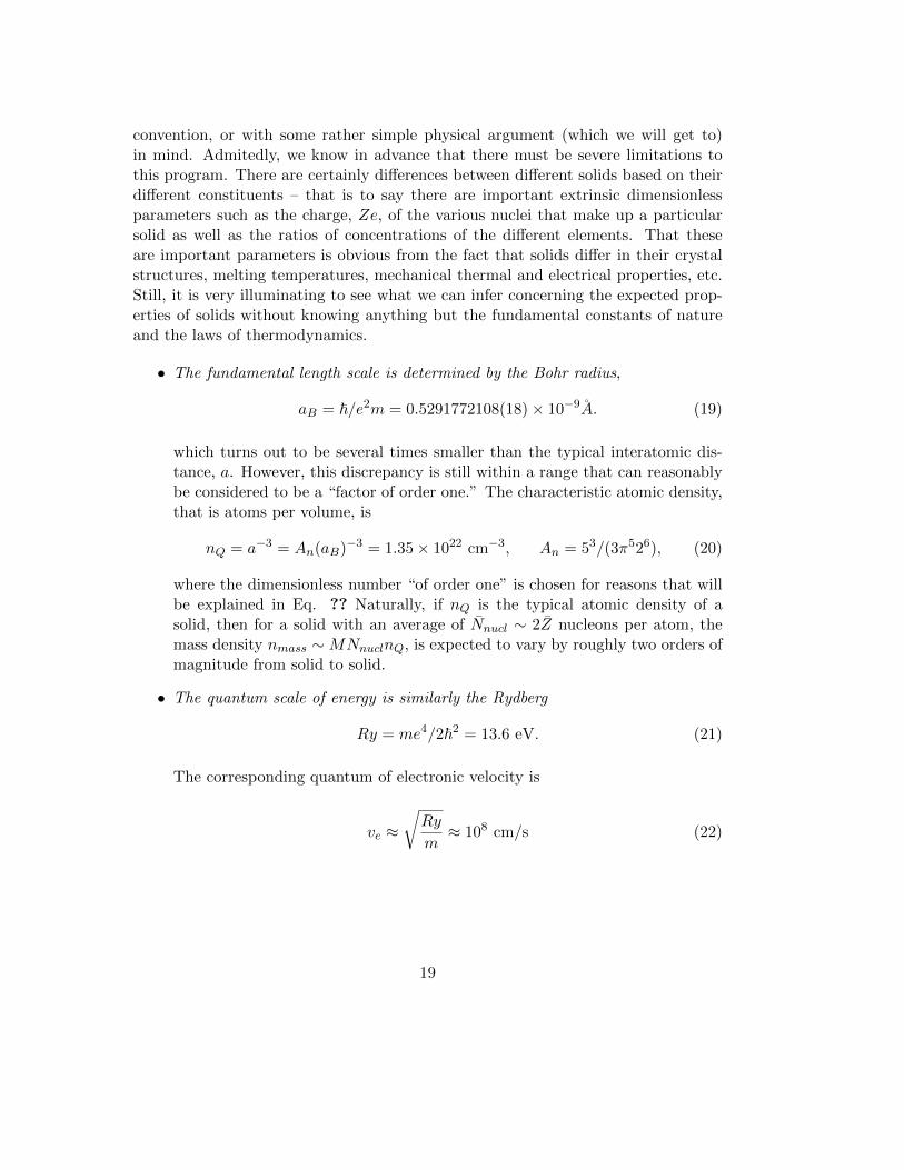
convention, or with some rather simple physical argument (which we will get to)in mind. Admitedly, we know in advance that there must be severe limitations tothis program. There are certainly differences between different solids based on theirdifferent constituents – that is to say there are important extrinsic dimensionlessparameters such as the charge, Ze, of the various nuclei that make up a particularsolid as well as the ratios of concentrations of the different elements. That theseare important parameters is obvious from the fact that solids differ in their crystalstructures, melting temperatures, mechanical thermal and electrical properties, etc.Still, it is very illuminating to see what we can infer concerning the expected prop-erties of solids without knowing anything but the fundamental constants of natureand the laws of thermodynamics.

• The fundamental length scale is determined by the Bohr radius,

aB = ~/e2m = 0.5291772108(18)× 10−9A. (19)

which turns out to be several times smaller than the typical interatomic dis-tance, a. However, this discrepancy is still within a range that can reasonablybe considered to be a “factor of order one.” The characteristic atomic density,that is atoms per volume, is

nQ = a−3 = An(aB)−3 = 1.35× 1022 cm−3, An = 53/(3π526), (20)

where the dimensionless number “of order one” is chosen for reasons that willbe explained in Eq. ?? Naturally, if nQ is the typical atomic density of asolid, then for a solid with an average of Nnucl ∼ 2Z nucleons per atom, themass density nmass ∼MNnuclnQ, is expected to vary by roughly two orders ofmagnitude from solid to solid.

• The quantum scale of energy is similarly the Rydberg

Ry = me4/2~2 = 13.6 eV. (21)

The corresponding quantum of electronic velocity is

ve ≈√Ry

m≈ 108 cm/s (22)

19

• The response of the ions is very slow compared to the response of the electrons.A simple scaling of the velocity based on the mass ratio between the ionic andelectronic masses gives

vion ≈ ve ×√

m

Mion∼ 2Z−1/2 × 106 cm/s (23)

The above observations can lead us a long way in estimating various proper-ties of solids. Starting from the characteristic energy, the corresponding quantumtemperature of the electrons (kB is Boltzmann’s constant.) is

Te = Ry/kB ≈ 105 K. (24)

Similarly, an ionic temperature will be estimated from

Tion = ~ωion/kB ≈ 103 K. (25)

For both cases this argument implies the existence of an extrinsic small parameter,T/Te for the electrons and T/Tion for the ions which may affect the properties ofsolids, in much the same way as the intrinsic parameters discussed above do. Theimportance of this new small parameter becomes clear when we consider temperaturedependence of various properties of solids.

For example the specific heat per unit volume, which is characterized by thequantum value

CQ = kBnQ = 6.34nQ × 10−6RyK−1 ≈ 2× 10−28erg K−1 cm−3 (26)

However, since the third-law of thermodynamics requires that the specific heatmust vanish as T → 0, the low temperature specific heat of a solid cannot be simplyof order of CQ. Instead, a more sophisticated expectation is that

C ∼ AeCQ(T/Te)xe +AionCQ(T/Tion)xion for T/Te 1 and T/Tion 1 (27)

where Ae and Aion are constants of order unity, and both, xe > 0 and xion > 0,but in order to determine their values we need more than dimensional reasoning.For example, the type of statistics that should be employed for each type particlescan be used to determine those power laws. In the case of electrons we will seethat Fermi-Dirac statistics consideration for the electrons yields xe = 1, while Bose-Einstein statistics for the collective motion of the ions yields xion = 3.

Mechanical properties of solids are largely determined by the binding of atomstogether to form the solid. The compressibility (κ) and bulk modulous (B) are both

20

thermodynamic quantities characterized by the quantum relation BQ = nQ/Ry.However, the above discussion of the ionic characteristic velocity also allow us towrite

B ≈ v2ion × ρ ≈ v2ionnQMion ≈ 1011dynes cm−2. (28)

(For those who are rusty in thermodynamics B = 1/κ = −(1/V )∂P/∂V .)

Transport effects in metals and insulators introduce more complex issues involvingat best, near-equilibrium situations. First, a finite conductivity is possible in metals,which is accompanied by dissipation of power due to a finite resistance. Startingfrom Ohm’s law in which the current density is proportional to the applied electricfield: je = σE, where σ is the electrical conductivity of the metal. We rememberthat Ohm’s law is basically a diffusion equation in which the current density ofnumber particles is replaced by a charge current density (je = ej), and E representsthe gradient of an electrochemical potential ( E = −∇φ) that controls the diffusionof charges in the metal: j = −(σ/e)∇φ = −(σ/e2)〈[∂(eφ)/∂n]〉∇n. The diffusioncoefficient, D is therefore replaced by σ such that the scaling of the quantum ofconductivity is given by:

σQ = e2(nQRy

)DQ (29)

where DQ = ~/m is the quantum of diffusion of electrons. One sees immediatelythat

σQ = e2nQRy

~m≈ e2a3B

(h2

ma2B

)=e2

ha−1B (30)

The resistivity is the inverse of the conductivity, and when generalized to anydimensionality it yields:

ρQ ≡ (h/e2)(aB)D−2 (31)

wherein D = 3, ρQ = 136.6 µΩ cm, (32)

andin D = 2, ρQ = h/e2 = 25.813 kΩ. (33)

Indeed, liquid metals and metallic glasses tend to have resistivities that are oforder ρQ. However, crystalline metals tend to have resistivities that are ordersof magnitude smaller. For reasons that will become clear when we investigate themotion of electrons in crystal in detail, we generally express the failure of dimensional

21

analysis in terms of an emergent length-scale in the problem, `, which is called thethe mean-free path. In terms of the dimensionless ratio, aB/`,

ρ ∼ ρQ(aB/`). (34)

For a good metal, a low-temperature value of aB/` ∼ 10−4 is possible, leading to aresistivity lower than 0.2µΩ cm.

Similar to the electrical conductivity, the thermal conductivity in a metal dependson diffusion of heat (or entropy). The heat equation is again a diffusion equationrelating the heat current density (jq = (kBT )j) and temperature gradient: jq =−κ∇T . Thus we write: (kBT )j = −(κ/kB)〈[∂(kBT )/∂n]〉∇n. We note that whenheat diffuses through electrons, a unit entropy of kBT is transported for every chargee. similarly, a charge e diffuses whenever a temperature gradient produces a chemicalpotential difference kBT = eφ. Thus, the heat equation scales in the same way ascharge diffusion if κ/kB = cσ(kBT )/e2, where c is a numerical constant. This scalingargument leads to the result:

κ

σ= c

(kBe

)2

T with : c =π2

3(35)

**** the value of c is pulled from a hat. We need to identify it as a constant of order1 which, we will see later, takes the stated value.*****

Turn to magnetic properties of solids, we note that quantum mechanics provide uswith a fundamental magnetic moment for an electron, that is the Bohr Magneton:µB = ~e/2mc. If we succeeded to polarize all electrons in the solid the resultingmagnetization density will be nQµB. However, we know that the susceptibility ofmetals is only a fraction of this number. This result that is due to the quantumstatistics of electrons can easily be understood if we remember that a magneticmoment in a field acquire an energy µH. Thus, the magnetization density has tobe proportional to this energy, and to obtain a dimensionless quantity we use ourquantum energy to obtain:

M = nQµBµBH

Ry(36)

which yields an electonic susceptibility:

χe ≈nQµ

2B

Ry≈ 10−7 emu (37)

While this simple argument works for the conduction electrons in metals, coreelectrons that are part of the ions will behave in a different fashion to an applied

22

magnetic field. This, more delicate issue of diamagnetism will be discussed later.

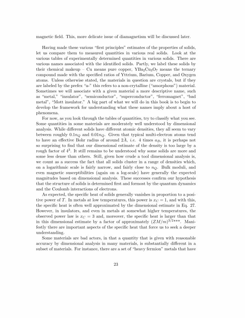
Having made these various “first principles” estimates of the properties of solids,let us compare them to measured quantities in various real solids. Look at thevarious tables of experimentally determined quantities in various solids. There arevarious names associated with the identified solids. Partly, we label these solids bytheir chemical makeup – Cu means pure copper, YBa2Cu3O7 means the ternarycompound made with the specified ratios of Yttrium, Barium, Copper, and Oxygenatoms. Unless otherwise stated, the materials in question are crystals, but if theyare labeled by the prefex “a-” this refers to a non-crytalline (“amorphous”) material.Sometimes we will associate with a given material a more descriptive name, suchas “metal,” “insulator”, “semiconductor”, “superconductor”, “ferromagnet”, “badmetal”, “Mott insulator.” A big part of what we will do in this book is to begin todevelop the framework for understanding what these names imply about a host ofphenomena.

For now, as you look through the tables of quantities, try to classify what you see.Some quantities in some materials are moderately well understood by dimensionalanalysis. While different solids have different atomic densities, they all seem to varybetween roughly 0.1nQ and 0.01nQ. Given that typical multi-electron atoms tendto have an effective Bohr radius of around 2A, i.e. 4 times aB, it is perhaps notso surprising to find that our dimensional estimate of the density is too large by arough factor of 43. It still remains to be understood why some solids are more andsome less dense than others. Still, given how crude a tool dimensional analysis is,we count as a success the fact that all solids cluster in a range of densities which,on a logarithmic scale is fairly narrow, and fairly close to nQ. Bulk moduli, andeven magnetic susceptibilities (again on a log-scale) have generally the expectedmagnitudes based on dimensional analysis. These successes confirm our hypothesisthat the structure of solids is determined first and formost by the quantum dynamicsand the Coulomb interactions of electrons.

As expected, the specific heat of solids generally vanishes in proportion to a posi-tive power of T . In metals at low temperatures, this power is xC = 1, and with this,the specific heat is often well approximated by the dimensional estimate in Eq. 27.However, in insulators, and even in metals at somewhat higher temperatures, theobserved power law is xC = 3 and, moreover, the specific heat is larger than thatin this dimensional estimate by a factor of approximately (ZM/m)3/2***. Mani-festly there are important aspects of the specific heat that force us to seek a deeperunderstanding.

Some materials are bad actors, in that a quantity that is given with reasonableaccuracy by dimensional analysis in many materials, is substantially different in asubset of materials. For instance, there are a set of “heavy fermion” metals that have

23

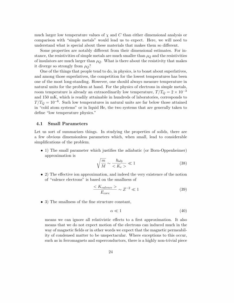
much larger low temperature values of χ and C than either dimensional analysis orcomparison with “simple metals” would lead us to expect. Here, we will need tounderstand what is special about these materials that makes them so different.

Some properties are notably different from their dimensional estimates. For in-stance, the resistivities of simple metals are much smaller than ρQ and the resistivitiesof insulators are much larger than ρQ. What is there about the resistivity that makesit diverge so strongly from ρQ?

One of the things that people tend to do, in physics, is to boast about superlatives,and among those superlatives, the competition for the lowest temperatures has beenone of the most long-standing. However, one should always measure temperature innatural units for the problem at hand. For the physics of electrons in simple metals,room temperature is already an extraordinarily low temperature, T/TQ = 2× 10−3

and 150 mK, which is readily attainable in hundreds of laboratories, corresponds toT/TQ = 10−6. Such low temperatures in natural units are far below those attainedin “cold atom systems” or in liquid He, the two systems that are generally taken todefine “low temperature physics.”

4.1 Small Parameters

Let us sort of summarizes things. In studying the properties of solids, there area few obvious dimensionless parameters which, when small, lead to considerablesimplifications of the problem.

• 1) The small parameter which justifies the adiabatic (or Born-Oppenheimer)approximation is √

m

M∼ ~ω0

< Ke > 1 (38)

• 2) The effective ion approximation, and indeed the very existence of the notionof “valence electrons” is based on the smallness of

< Kvalence >

Ecore∼ Z−2 1 (39)

• 3) The smallness of the fine structure constant,

α 1 (40)

means we can ignore all relativistic effects to a first approximation. It alsomeans that we do not expect motion of the electrons can induced much in theway of magnetic fields or in other words we expect that the magnetic permeabil-ity of condensed matter to be unspectacular. Where exceptions to this occur,such as in ferromagnets and superconductors, there is a highly non-trivial piece

24

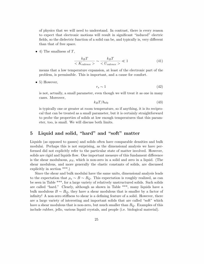
of physics that we will need to understand. In contrast, there is every reasonto expect that electronic motions will result in significant “induced” electricfields, so the dielectric function of a solid can be, and typically is, very differentthan that of free space.

• 4) The smallness of T ,

kBT

< Kvalence >∼ kBT

< Uvalence > 1 (41)

means that a low temperature expansion, at least of the electronic part of theproblem, is permissible. This is important, and a cause for comfort.

• 5) However,rs ∼ 1 (42)

is not, actually, a small parameter, even though we will treat it as one in manycases. Moreover,

kBT/~ω0 (43)

is typically one or greater at room temperature, so if anything, it is its recipro-cal that can be treated as a small parameter, but it is certainly straightforwardto probe the properties of solids at low enough temperatures that this param-eter, too, is small. We will discuss both limits.

5 Liquid and solid, “hard” and “soft” matter

Liquids (as opposed to gasses) and solids often have comparable densities and bulkmodulai. Perhaps this is not surprising, as the dimensional analysis we have per-formed did not explicitly refer to the particular state of matter involved. However,solids are rigid and liquids flow. One important measure of this fundament differenceis the shear moduluous, µS , which is non-zero in a solid and zero in a liquid. (Theshear modulous, and more generally the elastic constants of solids, are discussedexplicitly in section ***.)

Since the shear and bulk modulai have the same units, dimensional analysis leadsto the expectation that µs ∼ B ∼ BQ. This expectation is roughly realized, as canbe seen in Table ***, for a large variety of relatively unstructured solids. Such solidsare called “hard.” Clearly, although as shown in Table ***, many liquids have abulk modulous B ∼ BQ, they have a shear modulous that is smaller by a factor ofinfinity! A non-zero stiffness to shear is a defining feature of a solid. However, thereare a large variety of interesting and important solids that are called “soft” whichhave a shear modulous that is non-zero, but much smaller than BQ. Examples of thisinclude rubber, jello, various liquid crystals, and people (i.e. biological material).

25

The origin of the rigidity of solids is clearly a deep issue, and one that we willaddress as we delve into the subject. If one thinks about it from an atomisticviewpoint, it is almost unimaginable that when one applies a force to lift one endof a meter stick, the other end follows rigidly, the force being transferred from oneplane of atoms to the next for 1010 iterations. Even though the magnitude of µS cansometimes be successfully estimated by dimensional analysis, the rigidity itself is anemergent property that cannot be inferred by dimensional arguments alone.

Indeed, the existence of solids and gases can be inferred from dimensional anal-ysis: When T is large, entropy dominates the thermodynamics, and so one expectsgenerically to find gases - even nearly ideal gases. When T is small, the energy isdominant: since ions are more massive than electrons by the large factor ZM/m,the ion kinetic energy is typically negligible at T → 0, so matter in its groundstateis generally expected to be solid. (The notable exception to this, of course, is He atambient pressure, which remains a quantum fluid down to T = 0.) However, thereis no clear dimensional reason for the existence of a distinct liquid phase at inter-mediate temperatures, nor for the existence of soft condensed matter. It is certainlyfortunate that there is life beyond dimensional analysis!

6 Glassiness

7 Systems far from equilibrium

The most serious deficiency of this book (as far as we know) is that there is no discus-sion of systems far from equilibrium. As a moments reflection will certainly convinceyou, systems far from equilibrium are manifold among the most “intrinsically in-teresting” problems one would think of before being trained, in graduate school, tolimit ones curiosity to that small class of problems that physicists have been suc-cessful in treating. Systems in equilibrium are systems that are time independentand history independent, and this is rather boring. Systems far from equilibriumcan exhibit an extraordinary range of behaviors, including turbulent flow, spectac-ular pattern formation, and performances of Mozart operas. Since life is a highlynon-equilibrium phenomenon, and death is a large step towards equilibrium, thereare clear reasons to be more interested in systems far from equilibrium than systemsin or near equilibrium.

However, our understanding of non-equilibrium systems is far more primitivethan our understanding of equilibrium systems. In the course of this text, we willencounter many cases where we will draw the readers attention to even rather basicand fundamental aspects of the equilibrium properties of solids that are not under-stood. Still, there is much that is profound that we do understand about equilibriumsystems, and this is the subject of this text. Conversely, there is much about the

26

physics of systems far from equilibrium that is known, and known well enough thatwe can design airplanes that are stable in flight, predict many features of shock prop-agation in planetary magnetospheres, and can hope, someday, to generate electricpower from controlled fusion. More broadly, the study of systems far from equilib-rium is a great frontier of the subject, where open problems abound and fame andfortune await the brilliant young scientist who makes a significant contribution toour understanding of this subject.

27

***** What follows are notes that are still to be developed - mostly this will betables and figures showing the experimentally measured properties of solids.

8 Types of Solids

Crystalline solids and non-crystalline solids.(Covalent solids, ionic solids, molecular and polymeric solids, and composite ma-

terials.)

8.1 Walking through the periodic table what changes?

8.2 Phases of solids

Metal, insulator, superconductor, ferromagnet, commensurate and incommensuratecharge and spin density waves, ferroelectrics, quantized Hall fluids, ...

9 Properties of solids:

(In all cases, these should be compared to the corresponding quantum estimateobtained by dimensional analysis.)

9.1 Room temperature conductivity and resistivity at 4K or RR

9.2 Thermal conductivity of metals and insulators at low T and atroom T

(denote dominant mechanism).

9.3 Specific heats of metals and insulators

(C ∼ γT + βT 3, γ and β for metals, β for insulators).

9.4 Magnetic susceptibility broken into diamagnetic and param-agnetic parts

9.5 Density and compressibility of solids

9.6 Melting point of solids.

9.7 Electron Density

(by Hall number and other measures).

28

9.8 Speed of sound and Elastic Moduli in solids.

9.9 Dielectric constants of insulators.

9.10 Plasma frequencies of metals.

9.11 Gap magnitudes in semiconductors and insulators.

9.12 Magnitude of the electron-phonon coupling.

9.13 Dimensionless ratios Wilson Ratio, Weideman Franz ratio.

9.14 Transition temperatures to low T ordered phases:

9.14.i Superconductors

9.14.ii Ferromagnets/antiferromagnets

9.14.iii CDW/SDW

29