IIIIl_lllIIgIllll'_

, / ,/i,¸ ._

WHC- SA- 1792-FP

Statistical Application ofGroundwater Monitoring Data

" at the Hanford Site

C.J. ChouV. G. JohnsonF. N. Hodges

DatePublished

September 1993

To Be PresentedatGeologicalSocietyofAmericaAnnualMeetingBoston,MassachusettsOctober25-28,1993

Prepared for the U.S. Department of EnergyOffice of Environmental Restorationand Waste Management

WestinghouseP.O. Box 1970Hanf0n:lCompanyRichland, Washington99352

HanfordOperationsandEngineeringContractorfor the" U.S.DepartmentofEnergyunderContractDE-AC06-87RL10930

Copyright License By acceptanceof this article,the publisherand/or recipientacknowledgesthe U.S. Government'srighttoretain a nonexclusive,royalty-freelicense in andto any copyrightcoveringthis paper.

Approvedfor PublicRelease

ABSTRACT

Effective use of groundwater monitoring data requires both statisticaland geohydrologic interpretations. At the Hanford Site in south-centralWashington state such interpretations are used for (I) detection monitoring,assessment monitoring, and/or corrective action at Resource Conservation andRecovery Act sites; (2) compliance testing for operational groundwatersurveillance; (3) impact assessments at active liquid-waste disposal sites;and (4) cleanup decisions at Comprehensive Environmental Response Compensationand Liability Act sites. Statistical tests such as the Kolmogorov-Smirnov two-sample test are used to test the hypothesis that chemical concentrations fromspatially distinct subsets or populations (e.g., background area versuscontaminated or suspect site) are identical within the uppermost unconfined

" aquifer. Experience at the Hanford Site in applying groundwater backgrounddata indicates that background must be considered as a statisticaldistribution of concentrations, rather than a single value or threshold. Theuse of a single numerical value as a background-based standard ignoresimportant information and may result in excessive or unnecessary remediation.Appropriate statistical evaluation techniques include Wilcoxon rank sum test,Quantile test, "hot spot" comparisons, and Kolmogorov-Smirnov types of tests.Application of such tests is illustrated with several case studies derivedfrom Hanford groundwater monitoring programs. To avoid possible misuse ofsuch data, an understanding of the limitations is needed. In addition tostatistical test procedures, geochemical, and hydrologic considerations areintegral parts of the decision process. For this purpose a phased approach isrecommended that proceeds from simple to the more complex, and from anoverview to detailed analysis.

CONTENTS

I. 0 I NTRODUCTI ON ........................... I

2.0 STATISTICALANALYSIS TECHNIQUES_ . _. ............... i2.1 RANDOM EFFECTSMODELS -- VARIANCE

COMPONENTS ........... 42.2 ATTAINMENTOF A BACKGR(]Ur_D'BASED.....

CLEANUP STANDARD ....................... 8

3.0 CASE STUDIES .................. 133.1 CASE STUDY'I-'HANFORD'S-IOFACILITY" . ............ 143.2 CASE STUDY 2 - WELCOXON RANK TEST USING

• ARSENICTEST CASE ................ 163.3 CASE STUDY 3 - QUANTiLE iEST USING THE

ARSENIC TEST CASE ....................... 19

4.0 SUMMARYAND CONCLUSIONS....................... 21

5.0 REFERENCES ............................. 22

FIGURES:

I-I Locations of the RCRA GroundwaterMonitoringProjects and Landmarkson the Hanford Site ............. 2

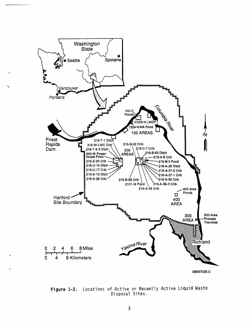
I-2 Locationsof Active or RecentlyActiveLiquid Waste Disposal Sites .................. 3

2-I A Shift Case Where the DistributionofMeasurementsfor a Contaminantof Concern inthe RemediatedWaste Site is ShiftedTwo Unitsto the Right of the BackgroundDistribution............. 10

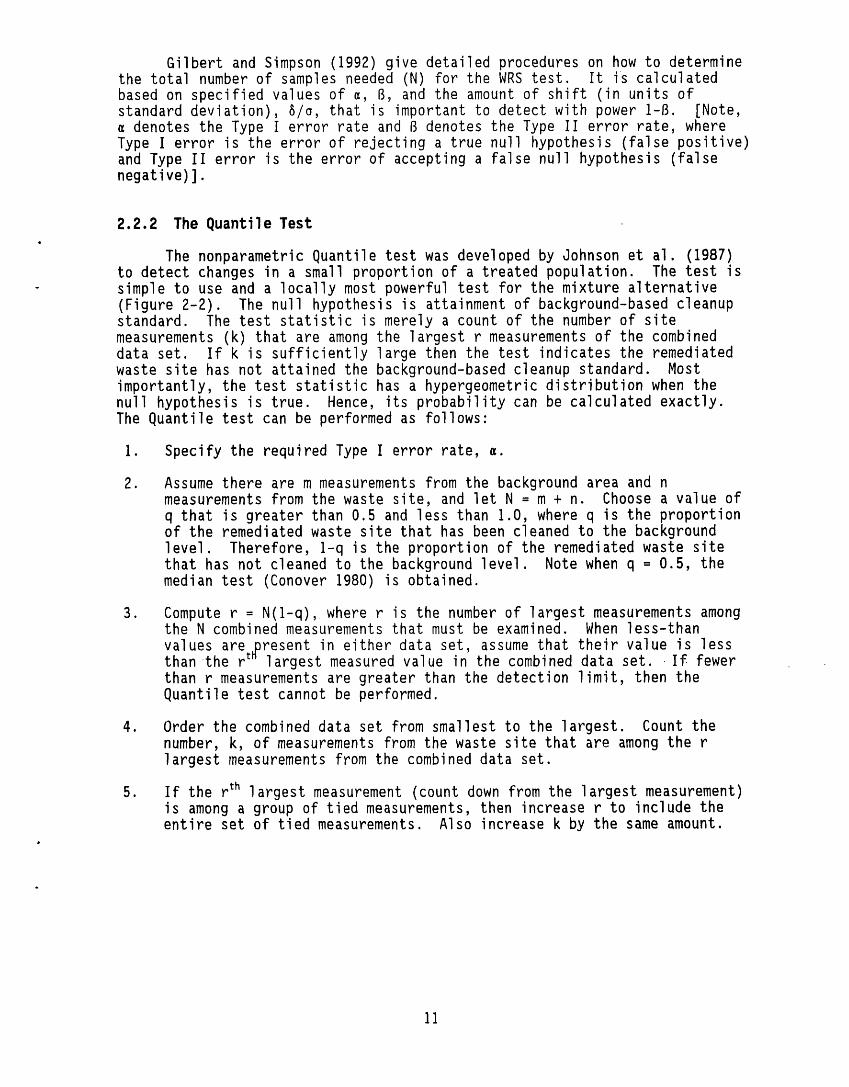
2-2 A Mixture Case Where 10% of the Distributionof Measurementsfor a Contaminantof Concernin the RemediatedWaste Site Has Not Cleanedto the BackgroundLevel ................... 12

3-I Monitoring Well LocationsOutside of KnownContaminationPlume Areas ................. 17

4-I A Phased Approach to Contamination/RemediationDecisions .............................. 23

TABLES:

I Analysis of Variance Table for a Two-WayCrossed Classification With a RandomEffects Model ....................... 5

- 2 A Nested RandomEffects Analysis of VarianceTable ................... 7

3 Background Specific Conductance I]ata a i_or £he- S-lO Facility ............................ 14

4 ANOVA for a Two-Way Crossed ClassificationsRandom Effect Model ................... 15

5 ANOVA for a Two-Way Nested CiassificationsRandom Effect Model ......................... 15

ii

CONTENTS (cont)

TABLES:

6 Arsenic Data From 10 Wells in the RattlesnakeMountain Corridor and 32 Wells Across theHanford Site ............... 18

7 Results of the'WRS Test--'Arsenic'Test Case ............. 20

iii

1.0 INTRODUCTION

Groundwater contamination problems at the U.S. Department of Energy(DOE) Hanford Site, in south-central Washington State, range from localgroundwater contamination associated with the individual waste disposal sitesto the overall impact of a 40-yr period of nuclear materials production andassociated contaminants released to the groundwater beneath the 1,450 km_site. Statistical analysis has been applied to groundwater contaminationproblems, which include (I) determining local backgrounds to ascertain whetheror not an individual disposal site is affecting the quality of groundwater,

L and (2) determining a "pre-Hanford" groundwater background for the HanfordSite to allow formulation of background-based cleanup standards. From thesestudies it is apparent that background for a specific analyte of concern

" should be considered as a statistical distribution, not as a single value orthreshold. Additionally, it is important to distinguish different sources ofvariation in the data and to handle them in the proper manner. If due care isnot exercised when determining background distributions there is a highprobability that false determinations of contamination will occur, resultingin unnecessary remediation and/or cleanup expense.

Effective use of groundwater monitoring data requires an integration ofstatistical and geohydrologic approaches. This combination is much moreeffective than either approach used in isolation. At the Hanford Site suchinterpretations are used for (I) detection monitoring, assessment monitoring,and/or corrective action at Resource Conservation and Recovery Act (RCRA)sites (Figure I-I), (2) compliance testing for operational groundwatersurveillance, (3) impact assessments at active liquid waste disposal sites(Figure I-2), and (4) cleanup decisions at Comprehensive EnvironmentalResponse Compensation and Liability Act (CERCLA)sites.

Statistical tests, such as the Kolmogorov-Smirnov two-sample test, havebeen used to test the null hypothesis that chemical concentrations fromspatially distinct subsets or populations (e.g., background area versushazardous waste site) are identical within the uppermost unconfined aquifer atthe Hanford Site (WHC1993). The primary purpose of this paper is tosupplement statistical methods discussed in WHC(1993) by (i) demonstratinghow to model spatial, temporal, and analytical variability of backgroundmeasurements, (2) showing that the variance estimate sz (that assumes equalspatial and temporal variability) is biased when multiple upgradient wellscomprise the background wells, (3) illustrating several statistical techniquesthat may be used in verifying the attainment of a background-based cleanupstandard (e.g., Wilcoxon rank sum test, quantile test, etc.); and(4) recommending an approach that represents some of the initial efforts inestablishing statistical guidance for evaluation of groundwater at the HanfordSite. Three case studies are provided.

2.0 STATISTICALANALYSISTECHNIQUES

w

Groundwaterquality informationis needed by regulatorsandenvironmentalmanagers for making decisionson assessingthe impact of afacility on groundwaterquality and/or the effectivenessof groundwaterremediationefforts. Over 250 RCRA-compliantgroundwatermonitoring wellshave been installedaround various facilitieson the Hanford Site since 1987,

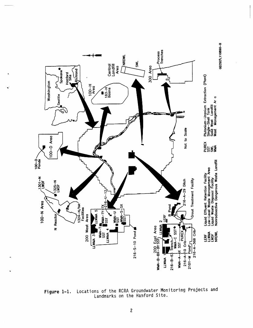
Figure I-I. Locationsof the RCRA GroundwaterMonitoring Projects andLandmarkson the HanfordSite.

WashingtonState

oSeattle Spokane

" Vancouver

,

Portland

1

•1325-N LWDF '_x_,..,1324-N/NAPond ,.-J

100AREAS -N-Priest 216-T-1 DI

Rapids 21

6-W-LWC Crib 216-B-62 Crib

200 \ 216-C-7 CribDam 216-T-4-2200.WPower-Ditch AREAS\ \ /216-B-63 Ditch

house Pond ' _t.._r.-.-..-216-A-8 Crib216-Z-20 Crl tL_qlJ.e :---- 216-B-3 Pond

216-U-14 Ditch _ __216-A-29 Ditch

216-S-10 Dltch_ / \ \ \ _'216-A-37-1 Crib216-S-26 Crib 216-B-55 Crib \ \ \ "216-A-30 Crib

2101-M Pofld _216-A-36-B Crib

216-A,_45Crib j400 Area )• Ponds

Hanford _ []400Site Boundary AREA

300 300AreaAREA

Trenches

_River Richland0 2 4 6 8Milesl I I = II I I I

0 4 8 Kilometers

L

$9007025.C

Figure I-2. Locationsof Active or RecentlyActive Liquid WasteDisposal Sites.

in addition to numerous older wells. At least 60,000 analytical results aregenerated annually for data evaluation and reporting.

From a statistical perspective, the null hypothesis of interest is thatthere is no difference in the chemical compositions of groundwater upgradient(background) and downgradient of a facility. However, the geohydrologiccond'itions at each site may be different, resulting in groundwater qualitydata that are highly site specific. Several statistical analysis techniquesthat model the background measurements (multiple upgradient wells, quarterlysampling events, and quadruplicate analysis results) into factors due tospatial, temporal, and analytical variabilities are provided. If background

• wells consist of several upgradient wells, the variance estimate s2 (whichassumes equal spatial and temporal variability) will underestimate the truevariance. The formula to calculate this bias is given for each model under

- consideration. Finally, non-parametric test procedures that are useful whenassessing the attainment of a background-based cleanup standard are presented.

2.1 RANDOM EFFECTS MODELS -- VARIANCE COMPONENTS

2.1.1 Crossed Classifications

In studying the variabilitythat is evident in the data, the maininterest is to attributethat variabilityto variousdata classifications.Classificationsthat identifythe source of each datum are called factors (orindependentvariables). The individualclasses of a factor are called levelsof that factor. A factor is random if its levels consist of a random sampleof levels from a populationof all possiblelevels, otherwise, it is fixed.In the context of groundwatermonitoring,the backgroundchemical compositionfor a particularanalyte of concern is usually obtainedfrom replicateanalysis of samplescollectedfrom multiple (e.g.,quarterly)sampling eventsof wells upgradientof the facility. When the locationsof the backgroundwells and the sampling times are assumedto be random variables,thebackgroundconcentrationcan be modeled by the followinggeneral equation"

Yijk = P + Wi + Tj + WTij + E(ij)k,

i = i, 2, ... a (numberof backgroundwells),j = i, 2, ... b (numberof samplingtimes),k = I, 2, ... r (numberof replicateanalyses),

where Yijkdenotes the kTM analysis on the jth samplingtime from the ithupgradientwell. Terms used in the model are defined as follows"

p : the true mean level for background measurements.

Wi = the true effect of the i th well. Wi is assumed to be a. random observation from a population with mean 0 and with

variance (_2W.

: the true effect of the jth sampling time. Tj is assumed toTj be a random observation from a population wlth zero mean and

with variance a2T.

WTij : the interaction between the i th well and jth sampling time.WT.. is assumed to be a random observation from a populationwi_;_ mean zero and with variance 02WT.

: the analytical error associated with the kth analysis ofE(tj)k

samples collected from well i at time j E(ij) K is assumedto be a random observation from a population with mean zeroand with variance O2A.

The above model assumes that all wells are measured at the same time.Therefore, the two factors (well and time) are referred to as "crossed"

T WTij, and Ecij)k are mutually. factors. It is also assumedthat the Wi, Js from a populationwith mean puncorrelated. Thus, each observationYijkand with variance

Var(Yijk)= O2w+ 02T + (12WT + CI2A.

The objective is to estimate the variousvariance components,o2w,0202 .T'.WT,and OA. The followinganalysisof variance (ANOVA)table (Table i) isglven to provide guidance in computingthe estimatesof these vari_hcecomponents.

Table I. Analysis of VarianceTable for a Two-Way CrossedClassificationWith a Random E:fectsModel.

,,,,

Source Degrees of Sum of MeanFreedom Squares Squares Expected Mean Squares

df SS MS E(MS), , ,,,

WeLL (a-l) SSW MSW a2A + ra2WT + rba2W

T_me (b-l) SST MST a2A + ra2wT + raa2T

We([ x Time (a-1)(b-1) SSwT MSwT a2A + ra2WT

Ana [yticaI ab( r-I) SSA MSA a2A,,, ,,,

Total abr-1 SSTota I,,.

Each mean square (MS) is obtained by dividing the sum of squares (SS) with therespectivedegrees of freedom (df). For example,MSW = SSw/(a-1),and

SSw : brZ:_ (7_.. - 7... )2,

SS T = ar_j (_.j.- _.. )2,

SSwT = r_j(_ij.-.V'-_..-_.j.+7...)2,

SS A = _i_j_,k(Yij k _ y'--j.)2,

. SSTota [ = _i_j_k(Yij k_ _...)2.

Note that the "." used in the above expression denotes the summation over a- particular subscript. For example, yi.. = _j_k-Tv'ijk and 7i.. = yi../br. Most

commercial statistical software packages will generate the quantities neededin the above table except for the expressions given in the expected meansquares column. A set of simple rules to determine these expressions quickly(without recourse to their derivation) is given in Hicks (1982).

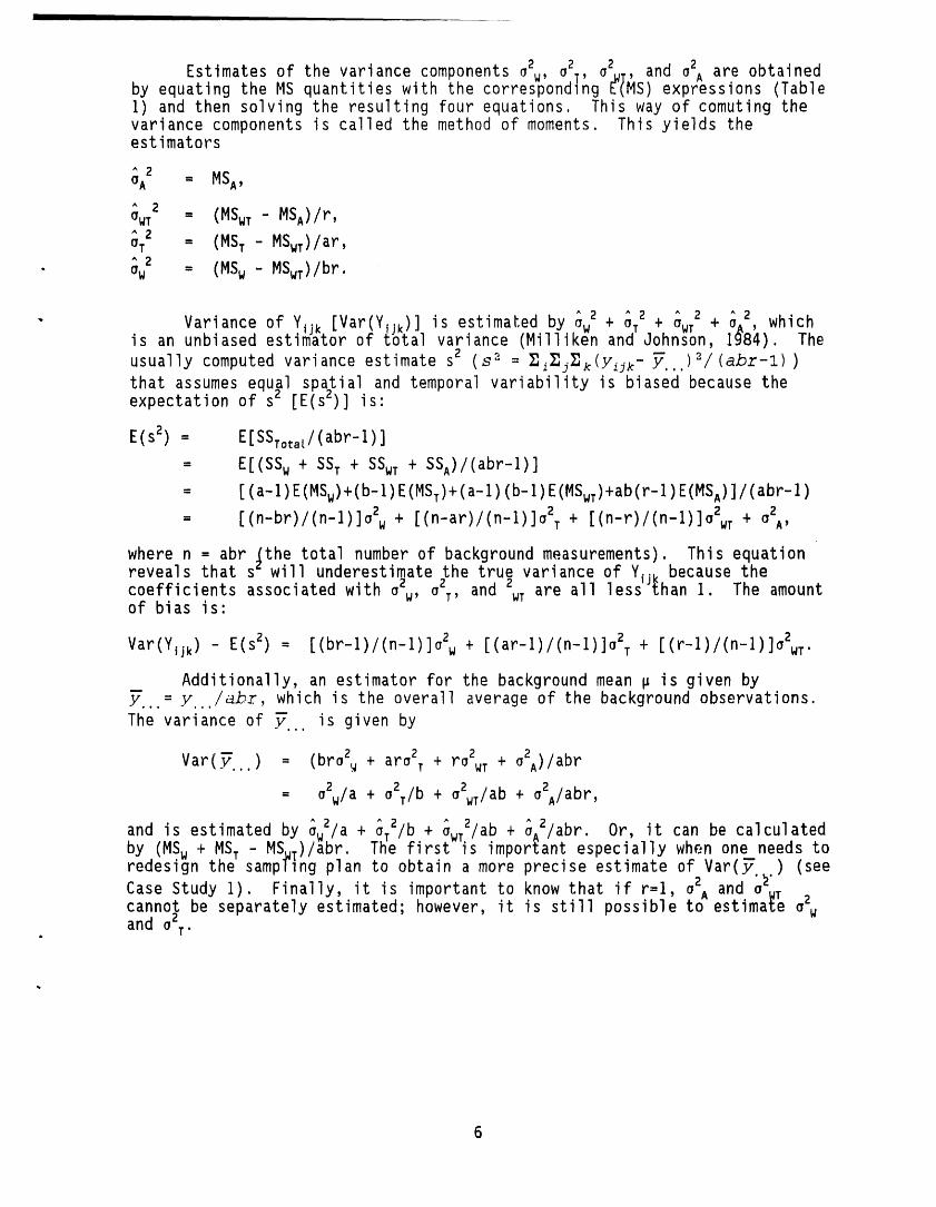
Estimatesof the variancecomponentso2w,o2T, a2_T,and a2Aare obtainedby equating the MS quantitieswith the correspondlngE"<MS)expressions (TableI) and then solvingthe resultingfour equations. This way of comuting thevariance components is called the method of moments. This yields theestimators

_A2 = MSA,

^ 2 = (MSwT- MSA)/r,OWTA

aTz = (MST - MSwT)/ar,

• _w2 = (MSW - MSwT)/br.

2 ^ ^ 2 ^ 2 )wh" Variance of Yijk.[Var(Yijk)]_isestimatedby _w + °T2 + °WT +io_ ichis an unbiased estlmazorof total variance (Millikenand Johnson, 8_$. The

usually computed variance estimate s2 (s2 = _,i_.j_k(yijk-_...)2/(abr_l))that assumes equal spatial and temporal variabilityis biased becausetheexpectationof s_ [E(s:)]is'

E(s2) = E[SSTota[/(abr-1)]

= E[(SSW + SST + SSwT+ SSA)/(abr-l)]

= [(a-l)E(MSw)+(b-I)E(MST)+(a-I)(b-I)E(MSwT)+ab(r-1)E(MSA)]/(abr-1)

= [(n-br)/(n-1)]O2w+ [(n-ar)/(n-l)]o2T+ [(n-r)/(n-l)]OzWT+ 02A,

where n = abr _the total number of backgroundmeasurements). This equationreveals that st will underestimatethe true variance of Y..-because the

coefficientsassociatedwith a2w, 02T,and 2WTare all lessIJ_hanI. The amountof bias is"

Var(Yijk)- E(sz) = [(br-l)/(n-1)]O2w+ [(ar-l)/(n-l)]O2T+ [(r-l)/(n-1)]_2WT.

Additionally,an estimatorfor the backgroundmean p is given by7...= y.../abr, which is the overall averageof the backgroundobservations.

The variance of 7... is given by

Var(7...) = (broZ_+ aro2T+ rO2WT+ O2A)/abr

= O2w/a+ O2T/b+ oZwT/ab+ a2A/abr,

and is estimatedby %/a + _T_/b+ %T_/ab + oA /abr. Or, it can be calculatedby (MS,+ MST - MSwT)/abr. The first is importantespeciallywhen one needs toredesign the sampTingplan to obtain a more precise estimate of Var(7 ) (see

Case Study I). Finally, it is importantto know that if r=1, a2Aand o21.cannot be separatelyestimated;however, it is still possible to estima{e o2wand 02T.

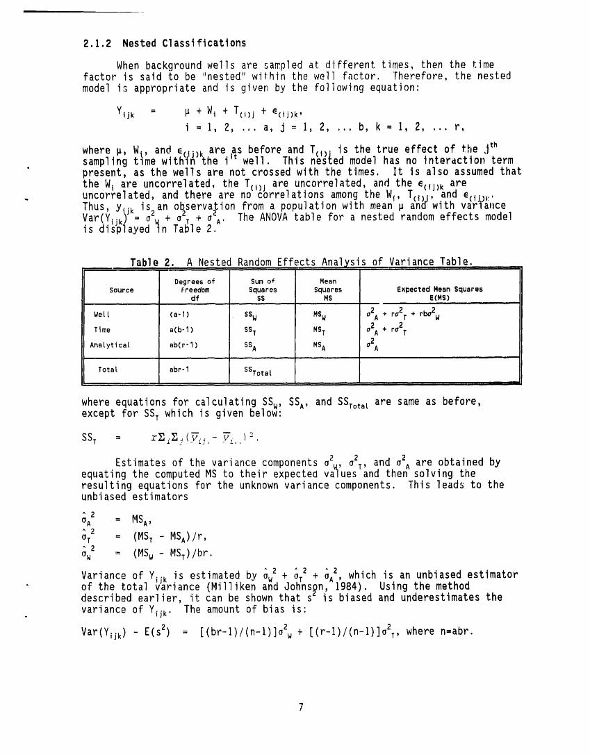
2.1.2 Nested Classifications

When backgroundwells are sampledat differenttimes, then the timefactor is said to be "nested"within the well Factor. Therefore,the nestedmodel is appropriateand is given by the followingequation:

Yljk = IJ + Wi + T(i)j + E(lj)k,

i = I, 2, .., a, j = I, 2, ... b, k = I, 2, .,. r,

where p, WI, and e • are as before and T(1)lis the true effect of the ,jthsampling me with(il_)ktheiitwell. This nested model has no interactionterm• present, as the wells are not crossed with the times. It is also assumed that

the W are uncorrelated,the T i are uncorrelated,and the el areI ( )j ( j)k. uncorrelated,and there are no correlationsamong the W(, Tci_i,and e(ll)).'

Thus, Y"k is an observationfrom a populationwith mean I_a'n_with vari'a,ceVar(YliklJ= azw+ aZT+ a2A. The ANOVA table for a nested random effects modelis dis'playedin Table 2.

Table 2 A Nested Random Ef:ectsAnalys s of Variance Table.i ] _: 41' iii iii iii ii|ll|m r i iii i i ,[ ,1.... ii i 1 iiii i!llllllllllllI i i/lllllll 11111I it i TF _ _

Degreesof Sum of MeanSource Freedom Squares Squares Expected Mean Squares

df SS MS E(MS),. , ,,.,.. i , f, ,, ,,,. i i , ,,. i

Wetl (a-l) SSW MSW o2A + ro2T + rbo2W

Time a(b-1) SST MST o2A + ro2T

Analytical ab(r-I) SSA MSA o2A... , ,,,.. ,,,,,,, ,, , q ,i ,,,..., JJ

Total abr-1 SSTotat, ,'"' ' "''IT" : ' , ii,i i i,ii,ii iiHlmm nil i iIL ...... ---

where equations for calculatingSSW, SSA, and SSTotaL are same as before,except for SST which is given below:

SST = rT, iT_:(7_: ' - y_.,) _.

Estimatesof the variance componentso2,,O2T, and OZAare obtained byequating the computedMS to their expected vaWluesand then solving theresultingequations for the unknown variancecomponents. This leads to theunbiased estimators

^2a A = MSA,

2(IT = (MS T - MSA)/r,^ 2(Iw = (MS W - MS T)/br.

Variance of Y_k is estimatedby (Iw_ + aT + (IA, which is an unbiased estimator" of the total varlance (Millikanand Johnson, 1984). Using the method

describedearlier, it can be shown that s_ is biased and underestimatesthe

. variance of Yijk" The amount of bias is'

Var(Yijk)- E(sz) = [(br-l)/(n-l)]aZw+ [(r-l)/(n-l)](IZT,where n=abr.

Just llke the "crossed"case, an estimatorfor the overallbackgroundmean p can be obtained by _ = v _br, which is the overall average of the

backgroundobservations. The varianceof _.. is given by

Var(iT.,,) - (bro2w+ r_2T+ O2A)/abr

• a2w/a+ _2T/ab + O_A/abr

and is estimatedby Ow_/a+ _T2/ab+ aA2/abr. Or, it can be estimated byMSw/abr, This first result is importantespeciallywhen one needs to redesignthe sampllngplan to obtain a more preciseestimate of Var(7...). If spatial

' variabilityis the most dominant factor in the total variance components,themost effectiveway to reduce the uncertaintyin estimatingthe backgroundmeanis to increasethe number of backgroundwells. That is, to make Var(7...)I

^ 2

smaller, one has to make _w2/asmallerd. To make Ow/a smaller,one has toIncroasethe denominatora (note 'a enotes the number of backgroundwells).To offset the cost due to samplingof more wells, one can decrease the numberof sampling times and reduce the nulilberof replicateanalyses,especiallywhenthe cost associatedwith each chemical analysis is high.

2.1.3 Impact on GroundwaterMonitoring

Regardless of wheth_,rthe model is a "crossed"or "nested"model, s2 isa biased estimatorwhen multi.plebackgroundwells exist. In calculatingtolerance intervals,prediction intervals,and/or confidence intervals,

Var(Yljk_should be used rather than s2. Otherwise, the resultingcalculatedintervalswill be smaller. In groundwatermonitoring,an upper (I-a)i00%tolerancebound, calculated on the basis of backgroundmeasurements,is oftenrequiredby regulatorsFor use as a thresholdvalue where I-_ denotes thelevel of confidence. The thresholdvalue is used to determinethe presence orabsenceof contamination. Without consideringspatial and temporalvariabilitiesin the calculations,the resultingbounds will be tooconservative(i,e., too low). Decisionsbased on such bounds may lead to toomany false positive conclusions,and as a result,unnecessaryor excessiveremediation.

Z.2 ATTAINMENT OF A BACKGROUND-BASEDCLEANUPSTANDARD

After the groundwaterat a RCRA/CERCLAsite has been remediated, it isnecessary to determinewhether the remediationeffort has been successful(i,e,, verificationof cleanup). This determinationshould be statisticallybased, using appropriatestatisticalsamplingdesigns and tests. Appropriatestatisticaltests may include the Wilcoxon Rank Sum (WRS) test and/or theQuantile test dependingon the type of residualcontaminationscenarios(Gllbertand Simpson, 1990). If the remedial action has "uniformly"reducedcontaminationlevels (i.e.,the shift alternative),but not to backgrounde

levels, the WRS test should be used because it has greaterpower than thequantile test. However, if most of the cleanup unit has been remediated to

, background levels and only a few "hot spots" remain (i.e.,the mixturealternative),the quantile test is preferredbecause it has more power thanthe WRS test (Gilbertand Simpson, 1990).

2.2.1 The 14ilcoxon Rank SumTest

The Wilcoxon rank sum test may be used to test for a shift in location(Figure 2-I) between two independent populations (e.g., chemical concentrationfrom the background area and waste site). In the case of cleanupverification, the null hypothesis Ho to be tested is the attainment of thebackground-based cleanup standard and the alternative hypothesis H_ is thenon-attainment (i.e., a one-tailed test). The WRStest is performed in thefollowing steps:

I. Obtain two random samples of sizes m (from background area) and n (from• waste site). Let N : m + n.

2. Order the N data values as though they were obtained from the same" population.

3. Assign ranks to the ordered observations. Assign rank I to the smallestobservation and N to the largest. When several data values are exactlyequal to each other (i.e., tied), assign to each the average of theranks they would have received had there been no ties.

4. If some of the data values are less-than values, assume these values aretied at a value less than the smallest detected value in the combineddata set and follow the procedure for handling ties.

5. Total the ranks given to the n samples from the waste site. Denote thistotal as Wrs.

6. If m and n are less or equal to i0, compare Wrs to the appropriatecritical value (Tu) in Appendix 18 of Ostle and Malone (1988). RejectHo if Wr__>Tu, where Tu is the upper critical value for the selectedone-tailed a value (note, m is the level of significance of the test,usually a is set to be 0.05 or 5%).

7. If both m and n are larger than I0 and no ties are present, compute thelarge sample test statistic

Wrs- n(N+l)/2Zrs

[ran(iV+Z)/12] z/2

8. If both m and n are larger than I0 and ties are present, compute Zrsbased on the following equation:

Z_ : w_- n(N+z)/22 i/2{ (rim/12) [(N+I-Zjtj (tj-l)/N(N-I) ] }

whereinthe gjthisgrouthe;umber. of tied groups and tj is the number of tied data

9. Reject Ho and accept HaifZr[distribu->nzI":' where Z1.: is the (i-_)quantile of• the standard normal io .

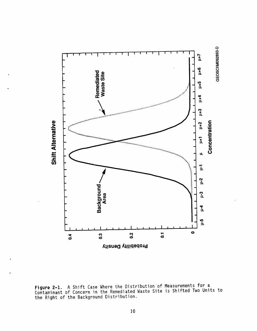
Figure 2-I. A Shift Case Where the Distributionof Measurementsfor aContaminantof Concern in the RemediatedWaste Site is Shifted Two Units tothe Right of the BackgroundDistribution.

10

Gilbert and Simpson (1992) give detailed procedures on how to determinethe total number of samples needed (N) for the WRStest. It is calculatedbased on specified values of _, B, and the amount of shift (in units ofstandard deviation), 8/o, that is important to detect with power I-8. [Note,

denotes the Type I error rate and 8 denotes the Type II error rate, whereType I error is the error of rejecting a true null hypothesis (false positive)and Type II error is the error of accepting a false null hypothesis (falsenegative)].

2.2.2 The Quantile Test

The nonparametric Quantile test was developed by Johnson et al. (1987)to detect changes in a small proportion of a treated population. The test is

- simple to use and a locally most powerful test for the mixture alternative(Figure 2-2). The null hypothesis is attainment of background-based cleanupstandard. The test statistic is merely a count of the number of sitemeasurements (k) that are among the largest r measurements of the combineddata set. If k is sufficiently large then the test indicates the remediatedwaste site has not attained the background-based cleanup standard. Mostimportantly, the test statistic has a hypergeometric distribution when thenull hypothesis is true. Hence, its probability can be calculated exactly.The Quantile test can be performed as follows:

I. Specify the required Type I error rate, a.

2. Assume there are m measurements from the background area and nmeasurements from the waste site, and let N : m + n. Choose a value ofq that is greater than 0.5 and less than 1.0, where q is the proportionof the remediated waste site that has been cleaned to the backgroundlevel. Therefore, l-q is the proportion of the remediated waste sitethat has not cleaned to the background level. Note when q : 0.5, themedian test (Conover 1980) is obtained.

3. Compute r : N(l-q), where r is the number of largest measurements amongthe N combined measurements that must be examined. When less-thanvalues are present in either data set, assume that their value is lessthan the r t"largest measured value in the combined data set. If fewerthan r measurements are greater than the detection limit, then theQuantile test cannot be performed.

4. Order the combined data set from smallest to the largest. Count thenumber, k, of measurements from the waste site that are among the rlargest measurements from the combined data set.

5. If the r th largest measurement (count down from the largest measurement)is among a group of tied measurements, then increase r to include theentire set of tied measurements. Also increase k by the same amount.

m

11

N

I /'=I , I , I,, - I ' o

_llSUeO ,_llllqeqoJd

Figure 2=2. A Mixture Case Where 10% of the Distributionof Measurementsfor a Contaminantof Concern in the RemediatedWaste Site Has Not Cleaned tothe Background Level.

12

6. If r_< 20, calculate the probability, P, of obtaining a value of k aslarge or larger than the observed k, if Ho is true

p: n-i i

(7) '(;)= a a- l a- l... s

over subscript i is from k, k+l, ..., r.

7. If r > 20, use the following equations to determine P, the probabilityof obtaining a value of k as large or larger than the observed k, if Hois true

X = r/rm+n

= mean of the hypergeometricdistribution

SD : [ mnr (m+n-r) ]i/2(m+n)2 (m+n-l)

= standarddeviationof the hypergeometricdistribution,and

k-O.5-xZp = SD , where Zp is a standard normal variable.

Use a standard normal distribution table with the computed value of Zpto determine the corresponding p value and let P = I - p.

8. Reject Ho and accept H_, if P < specified a. If Ho is rejected,conclude that the reme_diated waste site has not attained the backgroundstandard and additional remedial effort is needed.

Gilbert and Simpson (1992) gives a detailed description on how todetermine the number of samples based on computer simulations for the casewhere the residual contamination is assumed to be distributed at randomthroughout the cleanup site and the background and waste site measurements areassumed to be normally distributed. Look-up tables for conducting theQuantile test are also provided.

3.0 CASESTUDIES

Three case studies are provided in this section. The first case studyis to demonstrate the variance components analysis techniques describedearlier. The second and the third case studies illustrate the verification of

• cleanup efforts through the use of the WRStest and the Quantile test,respectively. Unless otherwise specified, the statistical software packageSTATGRAPHICS(Version 4.2) (a trademark of Statistical Graphics Corporation)was used to generate results presented in the ANOVAtables.

13

3.1 CASESTUDY1 - HANFORDS-lO FACILITY

Facility Background--The S-lO Facility is a RCRA-regulated treatment,storage, and disposal facility located south-southwest of the 200 West Area ofthe Hanford Site (see Figure 1-1). The S-10 Facility consists of a pond and aditch. In the past, it received waste water that contained dangerous wasteand radioactive materials from the Reduction-Oxidation Plant. The effluentstream to the S-tO Facility was permanently deactivated in October 1991.Currently, this facility is operated under the RCRAinterim-status regulations(EPA 1989).

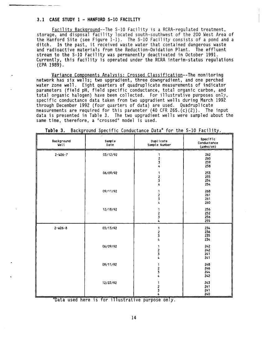
. VarianceComponents ..A.nal..ysis" Crossed Classification--The monitoringnetwork has six wells; two upgradient,three downgradient,and one perchedwater zone well. Eight quarters of quadruplicate measurements of indicatorparameters (fieldpH, field specific conductance,total organic carbon, andtotal organic halogen) have been collected. For illustrative purposes only,specific conductance data taken from two upgradient wells during March 1992through December 1992 (four quarters of data) are used. Quadruplicatemeasurements are required for this parameter (40 CFR 265.(c)(2)). The inputdata is presented in Table 3. The two upgradient wells were sampled about thesame time, therefore, a "crossed" model is used.

Table 3. BackgroundSpecific ConductanceDataa for the S-lO Facility.......

SpecificBackground Sample Duplicate Conductance

Welt Date Sample Number (_mho/cm)' ,,,i ,, ,,,,

2-W26-7 03/12/92 I 2622 2603 2594 258

06/09/92 1 2532 2553 2544 254

09/11/92 I 2682 2613 2614 260

12/18/92 I 2562 2523 2564 255

, , ,, , ,, , , ,,

2-W26-8 03/13/92 I 2342 2363 2354 234

06/09/92 I 2422 2423 2414 241

09/11/92 I 2482 2463 244

, 4 242

12/22/92 I 2432 2413 2414 240

_Data used h(_e"is "_or"ill'ustrat"vePurpose only.'

14

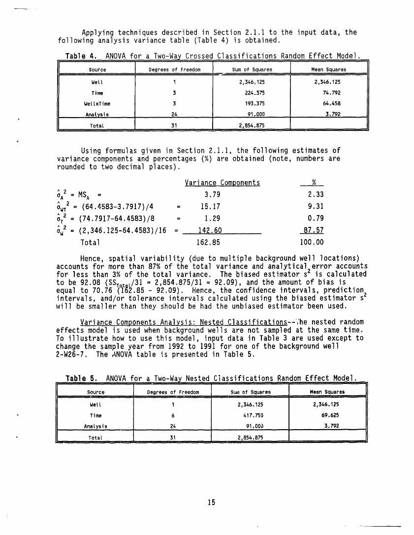
Applying techniquesdescribed in Section 2.1.1 to the input data, thefollowinganalysis variancetable (Table4) is obtained.

Table 4. ANOVA for a Two-Way CrossedClassificationsRandom Effect Model., , _ ,,,.

Source Degrees of Freedom Sumof Squares Mean Squares, .., , '" .... , ,,,,

WelI I 2,346.125 2,346.125

Time 3 224.375 74.792

WetlxTime 3 193.375 64.458

Analysis . 24 91.000 . .. 3;792=

Total 3!. 2,854.87S .....

Using formulas given in Section 2.1.1, the following estimates ofvariance components and percentages (%) are obtained (note, numbers arerounded to two decimal places).

Variance Components %A

aA2 = MSA = 3.79 2.33^ 2OwT = (64.4583-3.7917)/4 = 15.17 9.31^2oT = (74.7917-64.4583)/8 = 1.29 0.79

_w2 = (2,346.125-64.4583)/16= 142.60 87.57

Total 162.85 100.00

Hence, spatial variability(due to multiple backgroundwell locations)

accounts for more than 87% of the total varianceand analyticalerror accountsfor less than 3% of the total variance. The blased estimators_ is calculated

to be 92.08 (SSTotal/31= 2,854.875/31= 92.09), and the amount of bias isequal to 70.76 (162.85- 92.09). Hence, the confidenceintervals,predictionintervals,and/or tolerance intervalscalculatedusing the biased estimators2will be smaller than they should be had the unbiasedestimatorbeen used.

Variance ComponentsAnal.ys!s'Nested Classification_s--Thenested randomeffects model is used when backgroundwells are not sampled at the same time.To illustratehow to use this model, input data in Table 3 are used except tochange the sample year from 1992 to 1991 for one of the backgroundwell2-W26-7. The ANOVA table is presentedin Table 5.

Table 5. ANOVA for a Two-Way Nested ClassificationsRandom Effect Model.'ll , : "J_i i _ lll Z i _ T llr _:ii i P i TI II I I111III

I _OU_Ce 'I', Degrees of Freedom 1 Su_n of Squares [ M_an SquaresI'" ",' , ,r,,"_, . " ' ,.,, ,, , , r . ', : '_.,] = ,,.,, 'I ,.},,,

Weti I 2,346.125 2,346.125

• Time 6 417.750 69.625

..... Ana.lysis ........... 24 ..... 91.000 .... 3.792

Total 31 2,854.875III III II III II II 'I III I{ r i I111, I,'I_i I Iii_ ii I I i l.Ll ., --

15

I

Using formulas given in Section 2.1.2, the following estimates ofvariance components and (%) are obtained.

Variance Components %^

aA2 : MSA : 3.79 2.33^2aT = (69.625-3.792)/4 = 16.46 10.13

Ow2: (2,346.125-69.625)/16= 142.28 87.54

Total 162.53 100.00

• Just like the "crossed"case, spatial variabilityaccounts for more than87% of the total variance and only a small percent (less than 3%) of the totalvariabilityis due to analyticalerror. The total unbiased variance of

" backgroundmeasurementsis estimatedto be 162.53 (pmho/cm)2. A background

standard deviation of 12.75 (_mho/cm) (v/16p..53 = ].2.75) should be used whencalculating confidence intervals, prediction intervals, and/or toleranceintervals.

Let us use the more general "nested" model to show how to useinformation gained in the variance components analysis to design a futuresampling plan that will reduce the uncertainty associated with the estimatefor the overall background level. The overall background mean I_ is estimatedby

7...= _,i_,j_,_Y_jk/abr : 7,974/32 : 249 pmho/cm, and

Var(_...) is estimatedby MSw/abr= 2,346.125/32: 73.3 (pmho/cm)2. Or, itcan be estimatedby

¢w2/a ^ 2 ^ 2/ 142.28 + 16.46 + 3.79+ aT /ab + aA abr = -----a ab abr

This expression indicatesthat a more preciseestimate of Var(_...)will begained by increasingthe denominator 'a' (the number of backgroundwells)because spatial variabilityis the most dominant factor in calculatingthetotal variabilityof the data.

3.2 CASE STUDY 2 - WILCOXON RANK TEST USING ARSENIC TEST CASE

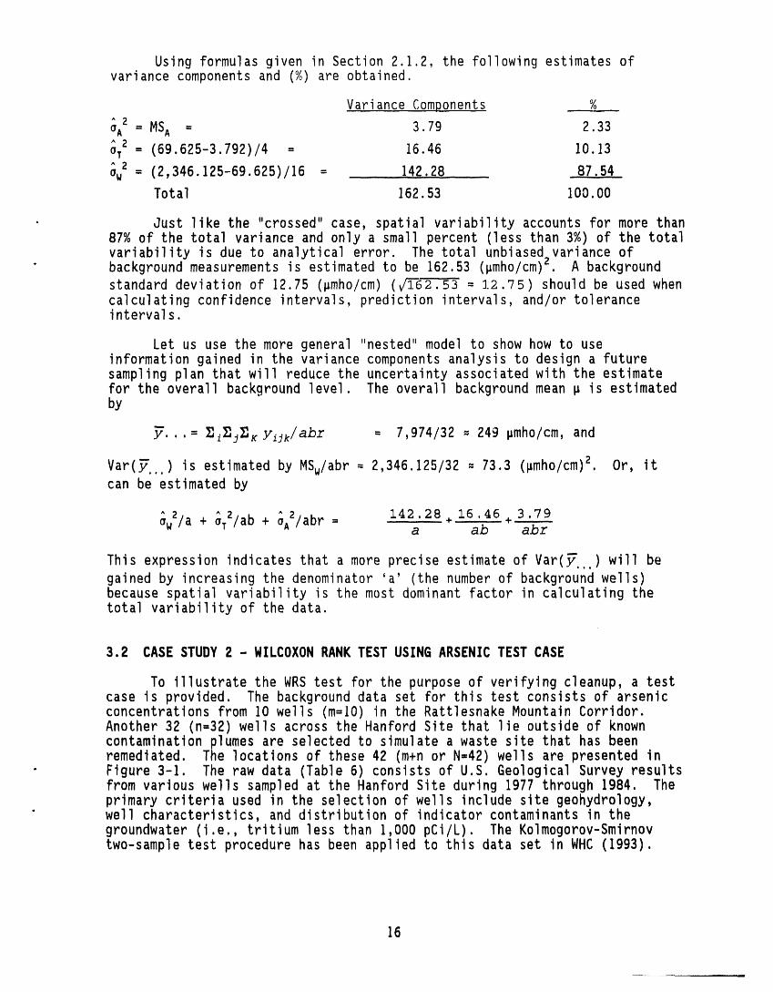
To illustratethe WRS test for the purpose of verifyingcleanup, a testcase is provided. The backgrounddata set for this test consists of arsenicconcentrationsfrom 10 wells (m:10) in the RattlesnakeMountain Corridor.Another 32 (n:32) wells across the HanfordSite that lie outside of knowncontaminationplumes are selected to simulate a waste site that has beenremediated. The locationsof these 42 (m+n or N-42) wells are presented in

• Figure 3-I. The raw data (Table6) consists of U.S. GeologicalSurvey resultsfrom various wells sampledat the Hanford Site during 1977 through 1984. Theprimary criteria used in the selectionof wells include site geohydrology,

" well characteristics,and distributionof indicatorcontaminantsin thegroundwater (i.e., tritium less than 1,000 pCi/L). The Kolmogorov-Smirnovtwo-sample test procedurehas been appliedto this data set in WHC (Igg3).

16

State Highway,24._

Figure 3-1. MonitoringWell LocationsOutsideof KnownContaminationPlumeAreas,Source:WHC (1993).

17

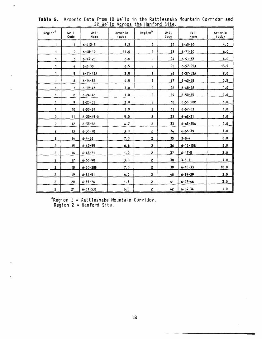
Table 6. Arsenic Data From I0 Wells in the RattlesnakeMountain Corridor and32 Wells Across the HanfordSite.

, _ ,_J ' - ..... = ', - _ ..,,. ....t_' ' !

Regiona J Welt We[[ i Arsenic l Regiona Well I Well ArsenicCode Name (ppb) Code Name (ppb)_I ' ,'. ,'I . "" " "'

I I 6-S12-3 5.5 2 22 6-45-69 4.0..., ,, ,, , , -

I 2 6-S8-19 11.0 2 23 6-71-30 6.0.,,, ,,,, , ,.,m ,. , , ,, ,,i

I 3 6-53-25 6.0 2 24 6-51-63 4.0,, ,=, , , ,, ,,, ,, ,. , i ,,. , .,, ,

I 4 6-2-33 6.5 2 25 6-57-25A 13.5,, ,, , ,,, , ,..,, , , ,=,..,

I 5 6-11-45A 3.0 2 26 6-37-82A 2.0" i,,, _i , ,,,,. ,n ,, i,i., ,,, --

I 6 6-14-38 4.0 2 27 6-43-88 0.5,.., .,,, ,., , , ,,

. .. I 7 6-19-43 3.0 ........2 .... 28 6-48-18 ....... 1.0

I . 8 6-24-46 1.0 2 29 .....6-50-85 ..... 2.0

....1 9 6725.55 3.0 ........ 2 30 ....6-_5-S0c............ 3.0I 10 6-55-89 1.0 2 31 6-57-83 1.0,,. i , , . . f,. , ,,.

2 11 6-20-E5-0 5.0 2 32 6-62-31 1.0_ ,,,i ,, ,,,, ,, ,,, ,,,, , " ', --

..... 2 12 6-33-56 .... 4.7 2 33 6-63"25A........ 4.0

2 13 6-35-78 3.0 2 34 6-66-39 1.0,. i ,,,,, , .. H, , i , --

2 14 6-4-86 7.0 2 35 3-8-4 8.0

2 15 6-49-55 6.6 ...... 2 36 6Z15-15B . 8.0_

2 16 6-48-71 1.0 2 37 ..6-17-5 ..... 3_0 _

_ 2 ...... 17 , 6-63-90 .......... 3.0 2 38 3-3-1 ...... 1,0

-- 2 _ 18 6"50"288 7"0 .... 2 .... 39 6"40"33 .......10.0

.......2 19 6-34-51 6...0 .... 2 40 , 6-39-39 ...... 2.0

2 20 6-55-76 1.3 2 41 6-4?-46 3.0.,. i, , , i ill ,,, ,,i, ,. ii, i i ,, , --

2 21 6-31-538 6.0 2 42 6-54-34 1.0,,,,_ ii,,,,," ,,,,, ", _, ,T : , ',, :z u ,,, ' • • '[ , ,,, L

aRegionI = RattlesnakeMountainCorridor,Region 2 = Hanford Site.

18

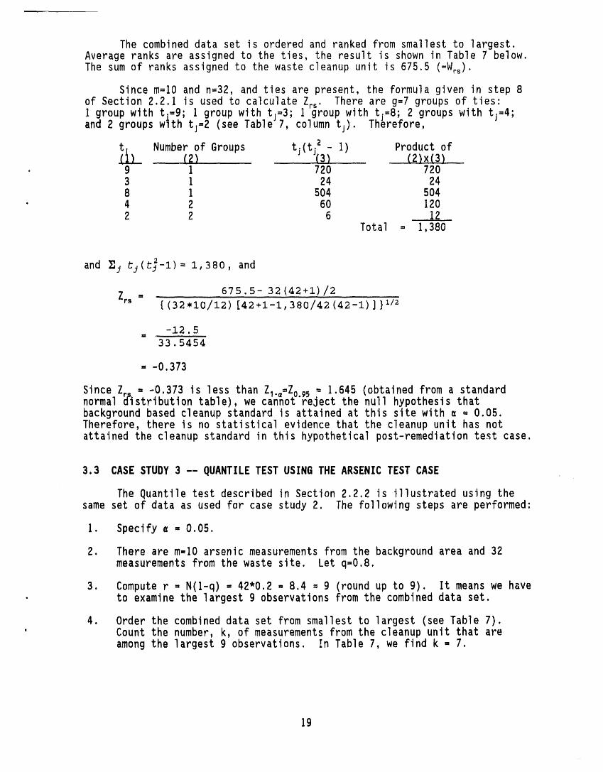
The combined data set is ordered and ranked from smallestto largest.Average ranks are assigned to the ties, the result is shown in Table 7 below.The sum of ranks assigned to the waste cleanup unit is 675.5 (=Wrs).

Since m=10 and n=32, and ties are present,the formulagiven in step 8of Section 2.2.1 is used to calculateZrs. There are g=7 groups of ties:i group with tl:9; I group with tj:3; I group with tj:8; 2 groups with tj:4;and 2 groups wlth tj=2 (see Table 7, column tj). Therefore,

tl Number of Groups tj(tj23-()I) Productof.... (2) ( 2 ) x ( 3 ) _

. 9 I 720 7203 I 24 248 I 504 504

• 4 2 60 1202 2 6 12

Total : .....1,380

and _j t_(t_-l) = 1,380, and

675.5- 32(42+i)/2ZpB _"

{(32,10/12) [42+1-1,380/42 (42-1) ]}i/2

-12.533.5454

= -0.373

Since Z =-0.373 is less than Zl.e=Zo.gs= 1.645 (obtainedfrom a standardnormal [{istributiontable),we cannot reject the null hypothesisthatbackgroundbased cleanup standard is attainedat this site with _ = 0.05.Therefore,there is no statisticalevidence that the cleanup unit has notattained the cleanup standard in this hypotheticalpost-remediationtest case.

3.3 CASESTUDY3 -- QUANTILETEST USING THE ARSENICTEST CASE

The Quantile test described in Section 2.2.2 is illustratedusing thesame set of data as used for case study 2. The followingsteps are performed:

1. Specifya _ 0.05.

2. There are m=10 arsenicmeasurementsfrom the backgroundarea and 32measurementsfrom the waste site. Let q:O.8.

3. Compute r = N(I-q) = 42*0.2 _ 8.4 : g (round up to 9). It means we have• to examine the largest9 observationsfrom the combineddata set.

4. Order the combineddata set from smallestto largest (see Table 7).' Count the number, k, of measurementsfrom the cleanup unit that are

among the largest g observations. In Table 7, we find k = 7.

19

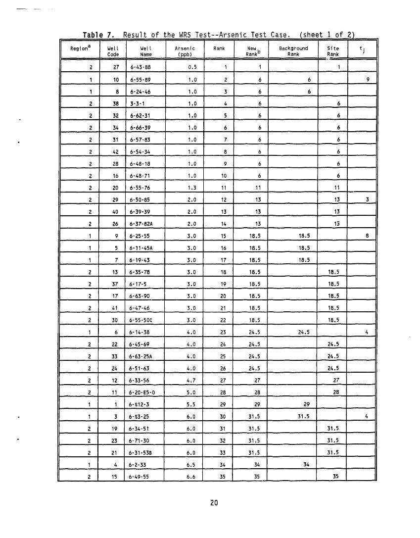
Table 7. Result of the WRS Test--ArsenicTest Case.,,,(sheet,I of,,,,,,2),, ..... ,I

Reglona Well Well Arsenic Rank Newb Background Site I t,,,Code ,,,Name (ppb),,,, ,,,, _,,_b Rank Rank I J

2 27 6"43"88 O.5 I I I, ,, ,, .... ,,. ,. ,, ,,

I 10 6-55-89 1.0 2 6 6 9,,, , ,, , ,, ,., ,

I 8 6-24-46 1.0 3 6 6, i J, , ,,,, ,, ,, , i ,.,

2 38 3-3-1 1.0 4 6 6i llml ,.. i,ii,i. .. i i,ii i,. , iii m i i,i|

2 32 6-62-31 i.0 5 6 6

2 34 6-66-39 I.0 6 6 6i,,i i . , , , . ,,, , ........

• 2 31 6-57-83 1.0 7 6 6, ,,,, ,, ,,, __

2 42 6-54-34 I.0 8 6 6,,, ,.- .. , ,,,. .. ,,. .

2 28 6-48-18 1.0 9 6 6

...... 2 II, 16 6"48-71 .......... 1.0 10 6 . j 6

2 20 6"55"76 1.3 11 11 11,.. ,,,, , , . , ,.,

2 29 6-50-85 2.0 12 13 13 3, |i ,,,, ,,,,,, ,,, ,.. , - .

2 40 6-39-39 2.0 13 13 13

2 26 6-37-82A 2.0 14 13 13,.., ,, , ,,

I 9 6-25-55 3.0 15 18,5 18.5 8,t ,., , , ,, ,,m i ,,

I 5 6-11-45A 3.0 16 18.5 18.5, ,,,, ,,., , ,,,,, .,, , •

I 7 6-19-43 3.0 17 18.5 18.5

2 13 6-35-78 3.0 18 18.5 18.5., ,,. ,,,. ,., ,..,

2 37 6-17-5 3.0 19 18.5 18.5. ,, ., , . ,,. , ,,

2 17 6-63-90 3.0 20 18.5 18.5l "

2 41 6-47-46 3.0 21 18.5 18.5... , , ,.,

2 30 6-55-50C 3.0 22 18.5 18.5,, , , ..... ,,,

I 6 6"14-38 4.0 23 24.5 24.5 4..... , ,.. . .

2 22 6-45-69 4.0 24 24.5 24.5i_ ,, , ,,., , ,,. , • ,,- -

2 33 6-63-25A 4.0 25 24.5 24.5, , ,, ,.. , , ,

2 24 6-51-63 4.0 26 24.5 24.5,,,, ,, , ,,,,. ,,,, .., .,, ,,, --

2 12 6-33-56 4.7 27 27 27 .... ]. ...

2 11 6-20-E5-0 5.0 28 28 28,...L , ,.,, , ,'

I I 6-$12-3 5.5 29 29 29

- I 3 6-$3-25 6.0 30 31.5 31.5 4

2 19 6-34-51 6.0 31 31.5 31.5, ,, • , , ,, ,,,. ..., , ,,

" 2 23 6-71-30 6.0 32 31.5 31.5,,.. ,

2 21 6-31-53B 6.0 33 31.5 31.5

I 4 6-2-33 6.5 34 34 34

2 15 6-49-55 6.6 35 35 35,..

20

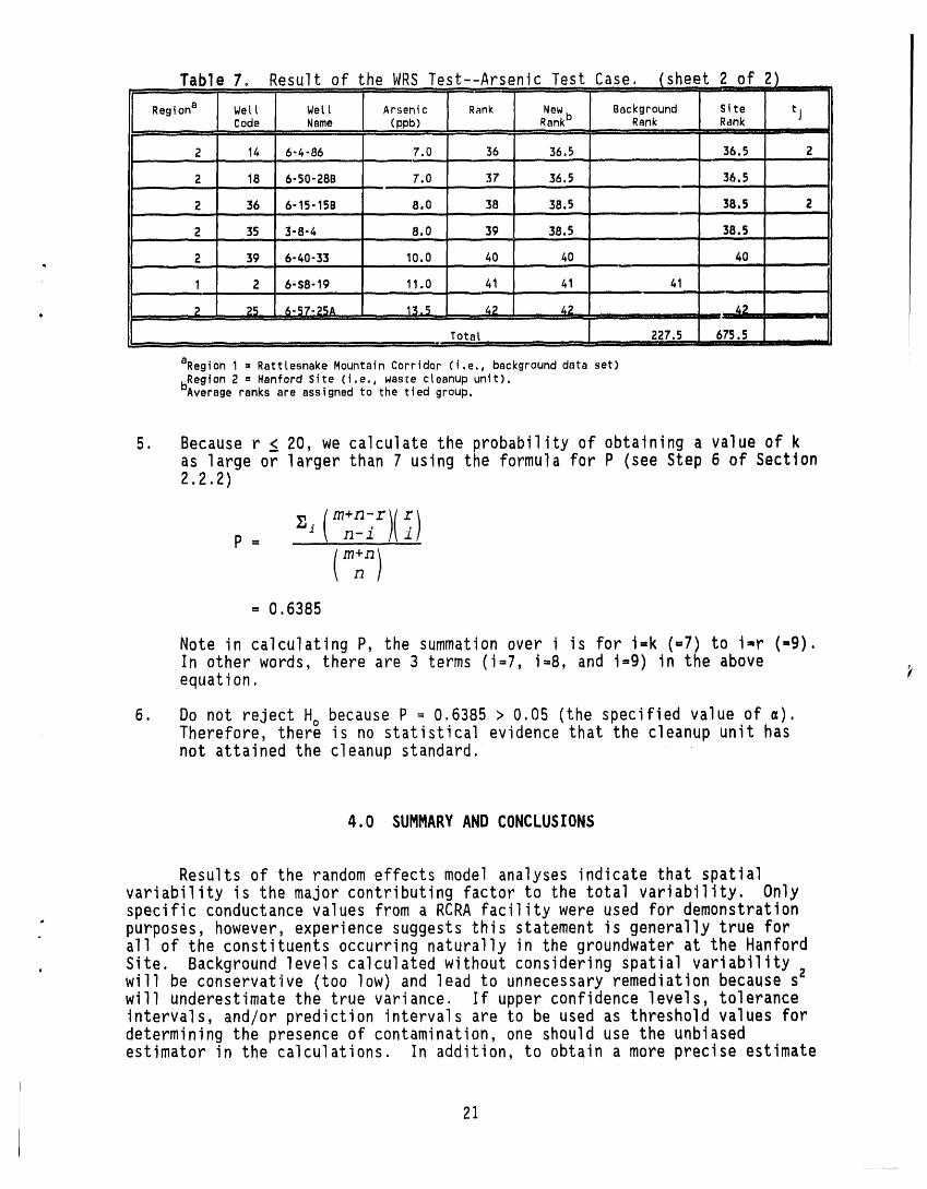
Table 7 Result of the WRS Test--ArsenicTest Case. (sheet 2 of 2)__ ,, _ : ....... '',c ,, , , , ,,,,,, , ,,,,, ,,,,,' , ,, :::

Code 1 Name (ppb) b Rank Rank

2 14 6-4-86 7.0 36 36.5 36.5 2,, , ± , ,,, , ,, ........ _ iil ,,i ......

, ,

2 18 6-50-28B T.O 37 36,5 36.5

2 36 6-15-i5B 8.0 38 38.5 38.5 2,, , .... ,,f i i,i ll,i1 H

2 35 3-8-4 8.0 39 38.5 38.5I II I I I I Illil IIII II iiJ]l IIIII I II I .....

, 2 39 6-40-33 10.0 40 4O....................... .__I 4 0 ___ __ ,,,, ,, ,,,,,,, , i ,,,,,,_ ,, i i i

I 2 6-S8-19 11.0 41 41 41,, ,,,,, i , i i i ,,

_ 2 25 6-57,25A 13.5 42 42 ..........42im ,, -, ,, ,, , ,, , ,,, ,,,, ,, , , ' ,,,,,,,, ,i, ',,L - ,,,

Total 227.5 675.5_ "" i I i i ii :_ _ I _ IIII I :: I I I_IiIIII I I _ : till ]I II IIH IIIIp!I I ] I -.: III !

aReglon I = RattlesnakeMountainCorridor (i.e.,backgrounddata set)bRegion 2 = HartfordSite (i.e.,wasce cleanupunit).Averageranks are assigned to the tied group.

5. Because r <_20, we calculatethe probabilityof obtaining a value of kas large or larger than 7 using the formulafor P (see Step 6 of Section2.2.2)

_,_ ( rn+n-r)( r)p= n-i i

m+nn)= O.6385

Note in calculatingP, the summationover i is for i=k (=7) to i-r (-9).In other words, there are 3 terms (i=7, i=8, and i=g) in the aboveequation.

6. Do not reject Ho because P = 0.6385 > 0.05 (the specifiedvalue of a).Therefore,there is no statisticalevidence that the cleanup unit hasnot attainedthe cleanup standard.

4.0 SUMMARYAND CONCLUSIONS

Resultsof the random effectsmodel analyses indicate that spatialvariabilityis the major contributingfactor to the total variability. Onlyspecific conductancevalues from a RCRA facilitywere used for demonstration

• purposes,however, experiencesuggests this statementis generallytrue forall of the constituentsoccurringnaturally in the groundwaterat the Hanford

. Site. Backgroundlevels calculatedwithout consideringspatial variabilitywill be conservative(too low) and lead to unnecessaryremediationbecause szwill underestimatethe true variance. If upper confidencelevels, toleranceintervals,and/or prediction intervalsare to be used as thresholdvalues fordeterminingthe presence of contamination,one should use the unbiasedestimator in the calculations. In addition,to obtain a more precise estimate

21

precise estimate of Var(_...), one should use the results of the variancecomponents analysis as a guide. For example, if spatial variability is themost important factor in the total variance components, the most effective wayto reduce the uncertainty in the estimation of background mean is to increasetho number of background we'lls. To offset the cost due to sampling of morewells, one can decrease the number of sampling times and reduce the number ofreplicate analyses, especially when the cost associated with each chemicalanalysis is high.

To effectively collect and utilize groundwater monitoring data in thefour programmatic areas at the Hanford Site, the background region should be

' selected from area(s) not influenced by the operations of the hazardous waste' site and similar to the test site in physical, chemical, or biological

characteristics. Furthermore, concentrations of chemicals in groundwater vary' considerably depending on factors such as soil characteristics, proximity to

recharge and discharge areas, and flow rates. Additionally, background shouldbe considered as a statistical distribution of concentration levels, ratherthan a single concentration, so that statistical techniques discussed in thispaper can be applied.

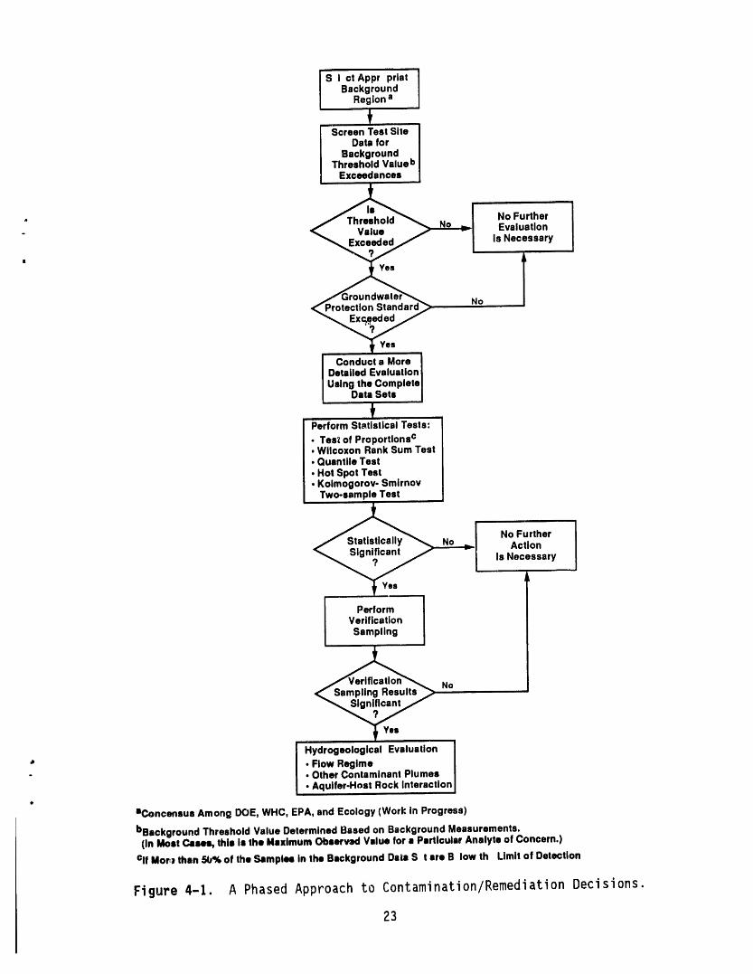
Finally, when making contamination and/or remediation decisions about awaste site, all available information must be used. In addition tostatistical test procedures, geochemical and hydrologic considerations areintegral parts of the decision making process. A phased approach, as shown inFigure 4-I, is recommended. The phases proceed from simple to the morecomplex, and from an overview to detailed analysis. All phases should becompleted and evaluated before a decision is reached. Work is in progresstoward this approach.

5.0 REFERENCES

Conover, W. J., 1980, Practical Nonparametric Statistics, Second Edition, JohnWiley and Sons, Inc., New York, New York, pp. 171, 216-223.

EPA, 1989, Interim Status Standards for Owners and Operators of HazardousWaste Treatment, Storage, and Disposal Facilities, Title 40, Code ofFederal Regulations, Part 265, as amended, U.S. Environmental ProtectionAgency, Washington, D.C.

Gilbert, R. O. and J. C. Simpson, 1990, Statistical Sampling Analysis Issuesand Needs for Testing Attainment of Background-Based Cleanup Standardsat Superfund Sites, PNL-SA-17907, Pacific Northwest Laboratory,Richland, Washington.

Gilbert, R. O. and J. C. Simpson, 1992, Statistical Methods for Evaluating the• Attainment of Cleanup Standards, Volume 3" Reference-Based Standards for• Soils and Solid Media, PNL-7409 Vol. 3, Rev.l, Pacific Northwest

Laboratory, Richland, Washington.o

Hicks, C. R., Fundamental Concepts in the Design of Experiments, ThirdEdition, CBSCollege Publishing, New York, New York, pp. 214-220.

22

S I ct Appr priatBackground

Regiona

Screen Test SiteDais for

BackgroundThreshold Value b

Excesdances

" _ No I No Further

ue _ EvaluationIs Necessary

• Tt v,.,

Conduct a MoreDetailed EvaluationUsing the Complete

Data Sets

Perform St_tistical Tests:

• Tesi of Proportionsc• Wllcoxon Rank Sum Test• Quantile Test• Hot Spot Test• Kolmogorov- Smirnov

Two-sample Test

No No FurtherActionIs Necessary

PerformVerificationSampling

No

Hydrogeological Evaluation

* • Flow Regime" • Other Contaminant Plumes

• Aquifer-Host Rock Interaction

aConcensus Among DOE, WHC, EPA, and Ecology (Work in Progress)

bBsckground Threshold Value Determined Based on Background Measurements.(In Most Cases, this is the Maximum Observ,ad Value for a Particular Analyte of Concern.)

Clf Mor,) than 5_% of the Samples In the Background Dale S t are B low th Limit of Detection

Figure 4-1. A Phased Approach to Contamination/RemediationDecisions.

23

Johnson, R. A., S. Verrill, and D. H. Moore II, 1987, "A Robust Two-StageMultiple Comparison Procedure with Application to a RandomDrug Screen."Biometrics 45:1281-1297.

Milliken, G. A. and D. E. Johnson, 1984, Analysis of Messy Data, Wadsworth,Inc., Belmont, California, pp. 212-273.

Ostle, B. and L. C. Malone, 1988, Statistics in Research, Basic Concepts andTechniques for Research Workers, Fourth Edition, lowa State UniversityPress, Ames, lowa, pp. 158-160, 636.

. WHC, 1993, Hydrologic CharacterizationPlan: I. PrincipalRecharge Zone forthe Hanford Site 200 Areas Waste Storage and Disposal Sites, Cold GreekValley Area, Western Hanford Site, WHC-SD-EN-AP-133,Westinghouse

• Hanford Company, Richland,Washington.

24

DISTRIBUTION

Number of copies

ONSITE

U.S. Departmentof En.erq.y-.1o Ri.chl.andO_e.rati.onsOffice.

R. D. Freeberg AB-IgM. J. Furman (4) A5-21

° J.M. Hennig A5-21- R.G. McLeod A5-19

R. P. Saget A5-52' Public Reading Room (2) AI-65

4 PacificNorthwest Laboratory

J. V. Borghese K6-g6M. A. Chamness K6-96S. S. Teel K6-96TechnicalFiles KI-11

58 Wes.tinqhouseHanford Company

D. J. Alexander H6-06D. B. Barnett H6-06D. J. Brown $I-06

J. A. Caggiano H6-06C. J. Chou (15) H6-06M. H. Edrington H6-06K. R. Fecht H6-06B. H. Ford H6-06P. B. Freeman H6-06M. J. Hartman H6-06F. N. Hodges (5) H6-06D. G. Horton H6-06R. L. Jackson H6-06V. G. Johnson (5) H6-06J. C. Johnston H6-06D. K. Jungers H6-06G. L. Kasza H6-06

A. J. Knepp H6-06A. G. Law H6-06R. B. Mercer H6-06R. E. Peterson H6-06S. P. Reidel H6-06V. J. Rohay H6-06

, J.S. Schmid H6-06• J.A. Serkowski H6-06

L. C. Swanson H6-06

' R.R. Thompson L4-96D. K. Tyler H6-06B. A. Williams H6-06InformationReleaseAdministration(3) H4-17Central Files (2) L8-04EPIC (2) H6-08

Distr-I